arctic ocean circulation patterns revealed by...

Arctic Ocean Circulation Patterns Revealed by GRACE

CECILIA PERALTA-FERRIZ AND JAMES H. MORISON

Polar Science Center, Applied Physics Laboratory, University of Washington, Seattle, Washington

JOHN M. WALLACE

Department of Atmospheric Sciences, University of Washington, Seattle, Washington

JENNIFER A. BONIN

College of Marine Science, University of South Florida, Tampa, Florida

JINLUN ZHANG

Polar Science Center, Applied Physics Laboratory, University of Washington, Seattle, Washington

(Manuscript received 19 December 2012, in final form 15 October 2013)

ABSTRACT

Measurements of ocean bottom pressure (OBP) anomalies from the satellitemissionGravity Recovery and

Climate Experiment (GRACE), complemented by information from two ocean models, are used to in-

vestigate the variations and distribution of the Arctic Ocean mass from 2002 through 2011. The forcing and

dynamics associated with the observed OBP changes are explored. Major findings are the identification

of three primary temporal–spatial modes of OBP variability at monthly-to-interannual time scales with the

following characteristics. Mode 1 (50% of the variance) is a wintertime basin-coherent Arctic mass change

forced by southerly winds through Fram Strait, and to a lesser extent through Bering Strait. These winds

generate northward geostrophic current anomalies that increase the mass in the Arctic Ocean. Mode 2 (20%)

reveals a mass change along the Siberian shelves, driven by surface Ekman transport and associated with the

Arctic Oscillation. Mode 3 (10%) reveals a mass dipole, with mass decreasing in the Chukchi, East Siberian,

and Laptev Seas, andmass increasing in the Barents andKara Seas. During the summer, themass decrease on

the East Siberian shelves is due to the basin-scale anticyclonic atmospheric circulation that removes mass

from the shelves via Ekman transport. During the winter, the forcing mechanisms include a large-scale cy-

clonic atmospheric circulation in the eastern-central Arctic that produces mass divergence into the Canada

Basin and theBarents Sea. In addition, strengthening of theBeaufort high tends to removemass from theEast

Siberian and Chukchi Seas. Supporting previous modeling results, the month-to-month variability in OBP

associated with each mode is predominantly of barotropic character.

1. Introduction

Arctic change has been reflected in decreasing sea ice

thickness (Kwok and Rothrock 2009), reduced summer

sea ice extent (Stroeve et al. 2007, 2008; Comiso 2012),

changed freshwater content and distribution (McPhee

et al. 2009; Rabe et al. 2011; Morison et al. 2012; Giles

et al. 2012), and increased atmospheric temperature

(Overland et al. 2008) and oceanic heat content (Steele

et al. 2008; Polyakov et al. 2010). Changes in all these

properties are of concern given their possible linkages

with global climate, for example by controlling stratifi-

cation in the sub-Arctic seas and thereby modulating

convection and the meridional overturning circulation

(Aagaard and Carmack 1989; Hu et al. 2010).

These changes have been linked to the Arctic Ocean

circulation and climate variability (Morison et al. 2000,

2006). During the late 1980s and early 1990s, the leading

mode of hemispheric surface atmospheric pressure, the

Arctic Oscillation (AO; Thompson and Wallace 1998),

entered an extreme positive phase. Positive AO is

Corresponding author address: Cecilia Peralta-Ferriz, Polar Sci-

ence Center, Applied Physics Laboratory, University of Washington,

1013 NE 40th St., Seattle, WA 98105.

E-mail: [email protected]

15 FEBRUARY 2014 PERALTA - FERR IZ ET AL . 1445

DOI: 10.1175/JCLI-D-13-00013.1

� 2014 American Meteorological Society

mailto:[email protected]

expressed as low surface atmospheric pressure over

the Arctic Ocean. During these years of positive AO,

the extent of the anticyclonic Beaufort high decreased,

leading to a counterclockwise shift of the transpolar drift

or zero vorticity line of sea ice motion (Rigor et al. 2002)

accompanied by a counterclockwise shift of the frontal

line between Pacific- and Atlantic-derived waters in the

central basin (Steele et al. 2004). This shift was consistent

with a salinity increase in the upper ocean of the central

Arctic (Morison et al. 2000). The cold halocline also

weakened and retreated counterclockwise (Steele and

Boyd 1998), enhancing melting of sea ice through the

increased ice exposure to warm Atlantic water. As the

atmospheric circulation directly affects sea ice motion,

the wind field associated with the positive AO increased

the export of multiyear ice through Fram Strait (Rigor

et al. 2002; Rigor and Wallace 2004).

During the early 2000s, the Arctic circulation relaxed

toward pre-1990s climatological conditions, including

a near-zero upper ocean salinity anomaly at the North

Pole (Morison et al. 2006). However, cyclonic high-AO

conditions appeared again after a positive jump in the

AO in 2007 (Morison et al. 2012).

To understand the rapid changes in the Arctic Ocean

and their role in climate change, it is necessary to learn

the basic patterns of circulation variation. Observations

by the National Aeronautics and Space Administration

(NASA) mission Gravity Recovery and Climate Experi-

ment (GRACE) of the time-varying mass field provide

a new approach tomeasure these patterns of change. Since

March of 2002, GRACE has provided essentially full

coverage of ocean bottom pressure (OBP) over the Arctic

Ocean. In this study, a decade ofGRACEand in situOBP

observations reveal the patterns of circulation change and

the unveiled forcing mechanisms are investigated using

output from two state-of-the-art ice–ocean models.

In what follows in section 2, the relevance of ocean

bottom pressure as a tool to understand ocean circulation

is presented, and background work on GRACE is in-

troduced. Section 3 describes the datasets and section 4

includes validation of satellite and models with in situ

observations. Section 5 shows the patterns of variability

of the GRACE bottom pressure field, and their associ-

ated forcing. A summary and conclusions are presented

in section 6.

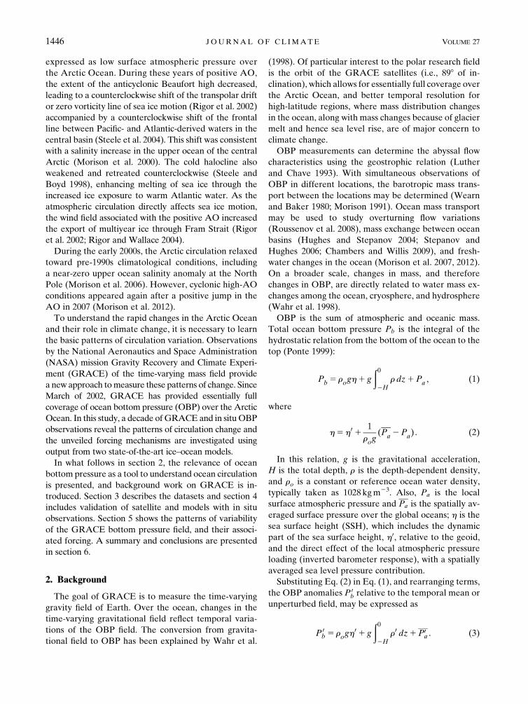
2. Background

The goal of GRACE is to measure the time-varying

gravity field of Earth. Over the ocean, changes in the

time-varying gravitational field reflect temporal varia-

tions of the OBP field. The conversion from gravita-

tional field to OBP has been explained by Wahr et al.

(1998). Of particular interest to the polar research field

is the orbit of the GRACE satellites (i.e., 898 of in-

clination), which allows for essentially full coverage over

the Arctic Ocean, and better temporal resolution for

high-latitude regions, where mass distribution changes

in the ocean, along with mass changes because of glacier

melt and hence sea level rise, are of major concern to

climate change.

OBP measurements can determine the abyssal flow

characteristics using the geostrophic relation (Luther

and Chave 1993). With simultaneous observations of

OBP in different locations, the barotropic mass trans-

port between the locations may be determined (Wearn

and Baker 1980; Morison 1991). Ocean mass transport

may be used to study overturning flow variations

(Roussenov et al. 2008), mass exchange between ocean

basins (Hughes and Stepanov 2004; Stepanov and

Hughes 2006; Chambers and Willis 2009), and fresh-

water changes in the ocean (Morison et al. 2007, 2012).

On a broader scale, changes in mass, and therefore

changes in OBP, are directly related to water mass ex-

changes among the ocean, cryosphere, and hydrosphere

(Wahr et al. 1998).

OBP is the sum of atmospheric and oceanic mass.

Total ocean bottom pressure Pb is the integral of the

hydrostatic relation from the bottom of the ocean to the

top (Ponte 1999):

Pb5 rogh1 g

ð02H

r dz1Pa , (1)

where

h5h0 11

rog(Pa2Pa) . (2)

In this relation, g is the gravitational acceleration,

H is the total depth, r is the depth-dependent density,

and ro is a constant or reference ocean water density,

typically taken as 1028 kgm23. Also, Pa is the local

surface atmospheric pressure and Pa is the spatially av-

eraged surface pressure over the global oceans; h is the

sea surface height (SSH), which includes the dynamic

part of the sea surface height, h0, relative to the geoid,

and the direct effect of the local atmospheric pressure

loading (inverted barometer response), with a spatially

averaged sea level pressure contribution.

Substituting Eq. (2) in Eq. (1), and rearranging terms,

the OBP anomalies P 0b relative to the temporal mean or

unperturbed field, may be expressed as

P 0b 5 rogh

0 1 g

ð02H

r0 dz1P0a . (3)

1446 JOURNAL OF CL IMATE VOLUME 27

The global-mean atmospheric pressure over the

ocean, P0a in Eq. (3), is usually neglected in most mod-

eling studies (Ponte 1999), mainly because it does not

lead to ocean dynamics. It does, however, affect the

global-meanOBP. Throughout this work, we will ignore

the global-mean SLP contribution, unless noted other-

wise (e.g., for consistency between model and observa-

tion comparisons). The first term on the right-hand side

in Eq. (3) is the contribution to the bottom pressure

change resulting from SSH variation. The second term

represents the bottom pressure contribution resulting

from the density variations of the water column. If two

of these three terms are known, then a complete picture

of the changes in the ocean circulation may be revealed.

In this work, we will sometimes refer to the pressure

resulting from the vertically integrated density term as

the steric pressure P0st. Following Gill and Niiler (1973),

steric pressure is the opposite sign of the steric height

anomaly,

h0steric52

1

ro

ð02H

r0 dz52P0st

rog, (4)

that results from the combination of the thermosteric

expansion and the halosteric contraction of the water

column. Because of the low coefficient of thermal ex-

pansion at low temperatures, the stratification of the

Arctic Ocean water column is dominated by salinity

rather than temperature: the thermosteric or temperature-

induced SSH change ismuch smaller than the halosteric or

salinity-induced SSH change.

Throughout this work, OBP variation will be referred

to in its normalized form (P0b/rog), and the units will be

provided in equivalent water thickness, such that 1mbar

(or 1 hPa) unit pressure corresponds to about 1 cm

equivalent water thickness.

Thus, following Eq. (3) and ignoring the atmospheric

term P0a, OBP has two contributions: the steric pressure

anomaly and the SSH anomaly. When the OBP change

is dominated by the SSH anomaly (e.g., OBP 5 SSH),

the ocean circulation is barotropic. When the steric

pressure becomes dominant, the relationship between

OBP and SSH breaks down, and the character of the

ocean circulation is baroclinic.

The dominance of the barotropic contribution over

the baroclinic contribution to OBP variations depends

on depth, latitude, time scale, and stratification (Gill and

Niiler 1973; Vinogradova et al. 2007; Bingham and

Hughes 2008). Modeling studies indicate that at high

latitudes (Vinogradova et al. 2007) and at the Arctic

Ocean in particular (Bingham and Hughes 2008), and

at annual and shorter time scales, the circulation is

predominantly barotropic, whereas at interannual and

longer time scales, circulation adjusts baroclinically.

Only in the shallow regions of the Arctic shelves (e.g.,

,200m) do the SSH fluctuations in the model of

Bingham andHughes (2008) remain coherent with OBP

fluctuations at longer than seasonal time scales.

Observations generally confirm the model results. Ice,

Cloud, and Land Elevation Satellite (ICESat) dynamic

ocean topography (DOT) h0 agrees with dynamic

heights relative to 500 dbar from in situ hydrography

(Kwok and Morison 2011), indicating the general

dominance of baroclinic adjustment. Recent trends in

ICESat DOT, GRACE OBP, and in situ hydrography

indicate that at multiyear time scales OBP changes

are mainly as a result of steric changes, and circulation

is largely baroclinic (Morison et al. 2012). Conversely,

GRACE and in situ observations of OBP suggest the

seasonal variations (Peralta-Ferriz and Morison 2010)

and submonthly variations (Peralta-Ferriz et al. 2011)

in Arctic Ocean mass are spatially coherent and baro-

tropic. Furthermore in a more recent study, Volkov

et al. (2013) used GRACE and altimetry observations

to quantify the sea level fluctuations in the Barents Sea

at different time scales, and demonstrated that at in-

traseasonal time scales, the mass-related variability of

sea level explains a large amount of the total sea level

change (e.g., OBP dominated by SSH instead of steric

pressure).

3. Data

a. GRACE ocean bottom pressure

In this work, we use GRACE release 4 data from

August 2002 to August 2011 as provided by the Uni-

versity of Texas, Center for Space Research (CSR) and

the Jet Propulsion Laboratory (JPL). (These data are

available online at ftp://podaac-ftp.jpl.nasa.gov/allData/

tellus/L3/ocean_mass/.)

GRACE OBP observations have become a powerful

tool for investigating ocean dynamics that have been

otherwise limited to sporadic locations or done with

only short-term observations. They have been validated

by several studies. Rietbroek et al. (2006) compared

GRACE OBP with pressure gauges in the Crozet-

Kerguelen region of the southern Indian Ocean, and

found significant correlation and that the signal-to-noise

ratio between GRACE and the difference of GRACE

minus in situ data was greater than one. Munekane

(2007) compared three years of GRACE OBP with five

in situ pressure sensors from the National Oceanic and

Atmospheric Administration (NOAA)’s Deep-Ocean

Assessment and Reporting of Tsunamis (DART)

gauges in the northeast Pacific Ocean and found good


ftp://podaac-ftp.jpl.nasa.gov/allData/tellus/L3/ocean_mass/

ftp://podaac-ftp.jpl.nasa.gov/allData/tellus/L3/ocean_mass/

correlations between the individual in situ data and the

GRACEOBP at each location. The average OBP of the

four most closely clustered pressure gauges showed an

RMS difference from GRACE OBP of 1.8 cm.

One study suggests that the signal-to-noise ratio of

GRACE OBP is largest at high latitudes (Kanzow et al.

2005). Since most of the Arctic Ocean falls under the

600-km footprint of GRACEmore often than do lower-

latitude regions, the potential to recover high-frequency

variations of OBP is greater, andmore accurate monthly

averages of OBPmay be obtained. Morison et al. (2007)

compared GRACE OBP at the North Pole to in situ

OBP measurements from two Arctic bottom pressure

recorders (ABPRs). The GRACE OBP and monthly

averages corresponding to the GRACE monthly values

agree to 2.6 cm. The GRACE–ABPR agreement at the

North Pole (R 5 0.75) highlights the tendency of

GRACE to generate more accurate measurements at

high latitudes compared to lower latitudes (Morison

et al. 2007; Kanzow et al. 2005). Monthly OBP obser-

vations from GRACE also show good agreement with

in situ observations in the Beaufort Sea and Fram Strait

(Peralta-Ferriz and Morison 2010).

For this study, data have been processed following

Chambers (2006a,b). The processing includes a correc-

tion for the postglacial rebound using the model of

Paulson et al. (2007), and a destriping algorithm

(Chambers 2006a) to remove the north–south propa-

gating errors of the gravity coefficients described by

Swenson and Wahr (2006). The data are also filtered

with a 300- or 500-km-radius Gaussian, and a spherical

harmonic filter cutoff at 408. Monthly means of the

Ocean Model for Circulation and Tides (OMCT) are

added back to the GRACE solutions to obtain the OBP

variations. A special algorithm is also applied to mini-

mize the leakage from land signals onto ocean signals.

There are four missing solutions out of the 109-month

record used because of technical issues with the

GRACE satellites. (More details on the GRACE sat-

ellite system may be found online at http://grace.jpl.

nasa.gov/.)

While Chambers (2006b) applied a correction for the

mass leakage from land into the ocean, strong signals

remained in the Arctic Ocean, particularly near the re-

gions of recent significant glacial mass loss (e.g., around

Greenland). An alternative method for removing the

land contamination of the ocean mass change by the

mass loss signals of Greenland and Svalbard has been

performed here (Bonin and Chambers 2013). This

method consists of separating the landmass and ocean

mass regions into several different basins, where each

basin is assumed to have constant mass density. Sixteen

basins are used across Greenland (eight in the coast, and

eight in the interior), with 13 other land regions (including

Iceland and Svalbard) and four ocean regions of semi-

coherent mass variation identified by the autocovariance

of the OMCT time series. From the GRACE data, least

squares estimation is used to solve for the mass signal in

each basin predicted to create that signal. The ‘‘forward

model’’ solution over the land basins is then smoothed

with either a 300- or 500-km-radius Gaussian filter, to

estimate the land leakage from those areas into the ocean.

This leakage estimate is removed from the original

GRACE solutions, producing a leakage-removed mass

signal.

We considered two GRACE postprocessed solutions

optimized in this way: 1) GRACE-300 was destriped

(Chambers 2006a) and smoothed with a 300-km radius

Gaussian filter, and 2) GRACE-500 was not destriped

but was smoothed with a 500-km radius Gaussian filter

(Fig. 1). The reasoning for considering a solution with-

out destriping follows the hypothesis that the larger filter

(500 km) may potentially eliminate the stripes without

introducing any artifacts resulting from the nonlinear

destriping algorithm (Bonin and Chambers 2013).

Comparison of trends from 2002 to 2009 ofGRACE-300

solutions and previous available solutions [e.g., version

dpc201012 by Chambers (2006b)] illustrate the effec-

tiveness of the optimization scheme in removing ter-

restrial mass change signal leakage into the ocean

domain, particularly around Greenland (Fig. 1). Away

from the regions of leakage optimization, GRACE-300,

GRACE-500, and the previously available solutions of

GRACE remain consistent in structure.

Overall, the GRACE-300 correlations with the

available in situ data (Table 1; data will be described in

the next section) were found to be slightly better than

theGRACE-500 correlations (Table 2), and the analysis

performed on GRACE-500 yielded results nearly

identical to the analysis performed on GRACE-300

(shown in sections to follow). Therefore, GRACE-300

with its better spatial resolution was selected to in-

vestigate the physical mechanisms associated with the

modes of OBP variability.

b. In situ pressure observations

Figure 2 shows the location of pressure and tide

gauges with data used in this work for validation of OBP

from GRACE and model output. The location of each

in situ record, length of the record, sampling frequency,

record gaps, and institution responsible for the data are

summarized in Table 1. All the tide and pressure gauge

records were detided and averaged daily and monthly.

All tide gauge data were corrected for the inverted-

barometer (IB) effect to yield the dynamic portion of

the SSH, using daily local sea level pressure (SLP) from


http://grace.jpl.nasa.gov/

http://grace.jpl.nasa.gov/

the National Centers for Environmental Prediction

(NCEP)–National Center for Atmospheric Research

(NCAR) reanalysis (Kalnay et al. 1996).

c. Atmospheric data

The atmospheric data used here consist of zonal and

meridional wind velocity fields at 925 hPa, and surface

atmospheric pressure from the NCEP–NCAR reanalysis

(Kalnay et al. 1996). (The data are available online at

http://www.esrl.noaa.gov/psd/.) Monthly averages from

2000 to 2011 are used. Monthly values of the Arctic

Oscillation Index are obtained from the NOAA/NCEP,

Climate Prediction Center (available online at http://

www.cpc.ncep.noaa.gov/products/precip/CWlink/daily_

ao_index/ao.shtml).

d. Models

We use monthly OBP and SSH output from two

ocean models, the Pan-Arctic–Ice Ocean Modeling

Assimilation System (PIOMAS) and Estimating the

Circulation and Climate of the Ocean, phase 2 (ECCO2;

phase 2 covers high-resolution global-ocean and sea ice

data synthesis).

PIOMAS is a regional ice-ocean model with 30 ver-

tical levels and spatial resolution better than 22 km

(Zhang and Rothrock 2003). The ‘‘North Pole’’ of the

PIOMAS model is located in northern Greenland, with

the goal of maximizing the resolution of flow exchange

in the region of Fram Strait. PIOMAS is one-way nested

to a global ocean model at 498N, and is forced by the

winds and surface atmospheric pressure from NCEP–

NCAR reanalysis data (Kalnay et al. 1996). Monthly

output of OBP and SSH anomalies are used from

January 2000 to December 2009.

ECCO2 was developed by the NASA Modeling,

Analysis, and Prediction (MAP) program. Synthesis

data for ECCO2 are obtained from the global ocean and

sea ice configuration of the Massachusetts Institute of

Technology general circulation model (MITgcm), and

the available in situ and satellite data. The optimized

FIG. 1. OBP trend (August 2002–December 2009) using CSR GRACE release 4 data

(a) destriped and smoothed with Gaussian filter of 300-km radius, processed by Chambers

(2006a); (b) destriped and smoothed with a 300-km-radius filter, and the optimized solution to

reduce land contamination as explained in the text; and (c) as in (b), but non-destriped and using

a 500-km-radius Gaussian filter.White contours show the International Bathymetric Chart of the

Arctic Ocean (IBCAO), version 2.23, data from Jakobsson et al. (2008), at 1000-m intervals.


http://www.esrl.noaa.gov/psd/

http://www.cpc.ncep.noaa.gov/products/precip/CWlink/daily_ao_index/ao.shtml



ECCO2 version (Nguyen et al. 2011) of the model used

here is forced with the Japanese 25-yr Reanalysis (JRA-

25) project. It has 50 vertical levels, and an average

spatial horizontal resolution of 18 km. Monthly output

of OBP and SSH anomalies are obtained from 2000

to 2009.

Both PIOMAS and ECCO2 use the Boussinesq ap-

proximation, and they have a true free surface height.

The modeled SSH is not affected by sea ice because

neither PIOMAS nor ECCO2 uses nonlinear freshwater

fluxes, nor do they use real freshwater fluxes. Instead,

they apply a correction to the salinity field (virtual salt

flux adjustment) by decreasing the salinity at most of

the river mouths. In PIOMAS, this adjustment is based

onmonthly climatological values of runoff input into the

ocean using values of runoff discharge from Hibler and

Bryan (1987). ECCO2 uses newer climatological values

of monthly-mean estuarine fluxes of freshwater, which

are based on the Regional, Electronic, Hydrographic

Data Network for the Arctic Region (R-ArcticNET)

dataset (Lammers et al. 2001). These values are further

adjusted for underestimated freshwater fluxes by mul-

tiplying for a factor of 1.2 (Nguyen et al. 2011). This

adjustment helps the freshwater budget of themodel to be

closer to other estimates (e.g., Serreze et al. 2006). Finally,

neither PIOMAS nor ECCO2 includes the global-mean

SLP, which is a term included in GRACEOBP. ECCO2

includes the global-mean freshwater cycle (A. Nguyen

2013, personal communication) but PIOMAS does not

(global-mean freshwater cycle equals global-mean OBP

minus global-mean SLP). Although these global-mean

contributions to OBP are small (RMS ; 0.5 cm) and are

strongly dominated by the seasonal cycle, they are taken

into account when comparing the different products of

OBP and SSH, as explained in the following sections.

4. Validation of GRACE and model OBP

a. GRACE–in situ comparison

GRACE-300 is validated with the available in situ

monthly averaged records from the stations shown in

Fig. 2. To do so, we linearly interpolated GRACE data

onto the locations of tide and pressure gauges. Before

we compare GRACE with the IB-corrected records

from tide gauges, we removed the global-mean SLP

TABLE 1. Stations of in situ pressure and tide gauges, location, length of record, sampling frequency, monthly record gaps, and source or

institution responsible.

Station Location Gauge type Temporal coverage

Sampling

frequency

Gaps

(month) Program or institution

North Pole 89815.260N, 60821.580E Pressure Apr 2005–Apr 2011 15min — North Pole Environmental

Observatory (NPEO)/University

of Washington (UW)

Beaufort

Sea

76859.230N, 139854.50W Pressure Aug 2003–Aug 2008 20min — Beaufort Gyre Exploration Project

(BGEP)/Woods Hole

Oceanographic Institution (WHOI)

Fram Strait 78849.930N, 580.870E Pressure Oct 2003–Dec 2010 20min 1 Alfred Wegener Institute (AWI) for

Polar and Marine Research

Bering Strait 65848.070N, 168847.90W Pressure Sep 2007–Sep 2009 20min — Russian–American Long-Term

Census of the Arctic

(RUSALCA)

Vardo 70819.80N, 31860E Tide Aug 2002–Dec 2009 Monthly — Arctic and Antarctic Research

Institute (AARI)/Permanent

Service for Mean Sea

Level (PSMSL)

Dunai 73855.80N, 1248300E Tide Aug 2002–Dec 2009 Monthly 2 AARI/PSMSL

Amderma 698450N, 618420E Tide Aug 2002–Dec 2009 Monthly 1 AARI/PSMSL

UST 698150N, 64831.20E Tide Aug 2002–Jan 2009 Monthly 11 AARI/PSMSL

Golomianyi 798330N, 90837.20E Tide Aug 2002–Jul 2009 Monthly 9 AARI/PSMSL

Kigiliah 73819.80N, 139852.20E Tide Aug 2002–Dec 2009 Monthly 1 AARI/PSMSL

Kotelnyi 768N, 137852.20E Tide Aug 2002–Dec 2009 Monthly 1 AARI/PSMSL

Pevek 698420N, 1708150E Tide Aug 2002–Dec 2009 Monthly 1 AARI/PSMSL

Sannikova 74839.60N, 1388540E Tide Sep 2002–Nov 2009 Monthly 3 AARI/PSMSL

Tiksi 71834.80N, 1288540E Tide Aug 2002–Dec 2009 Monthly — AARI/PSMSL

Tuktoyaktuk 69825.810N, 132859.40W Tide Sep 2003–Dec 2009 Hourly 10 Department of Fisheries and

Oceans (DFO), Canada

Holman 70844.210N, 117845.530W Tide Jan 2003–Apr 2008 Hourly 1 DFO, Canada

Alert 82829.510N, 628190W Tide Jan 2003–Jul 2009 Hourly 3 DFO, Canada


from GRACE for consistency with the tide gauges.

Figure 3 shows the time series comparisons between

GRACE OBP and in situ records for five locations: the

North Pole, Fram Strait, averaged tide gauge records in

the Kara Sea, averaged tide gauge records in the Laptev

Sea, and the Canadian Arctic at Alert Station (Fig. 3).

We averaged the records from the tide gauges located

in the Laptev and Kara Seas (see map in Fig. 2) to

remove the effects of localized processes of SSH change

in the coast and around islands. This averaging offers

a more realistic comparison with GRACE data, which

have undergone several smoothing steps and have

a large footprint (300-km radius).

The correlation between OBP from GRACE and the

in situ data is good, particularly with the in situ records

at the North Pole (R5 0.76), Fram Strait (R5 0.53), and

TABLE 2. Correlation coefficientR, RMS variability, andRMS difference between themonthly averaged tide or pressure gauge records

in the Arctic Ocean and GRACE, and between the in situ records and the model (RMSE). The seasonal variation was removed from all

the time series. For the model–observation correlations, the numbers in parentheses include the seasonal variation. All coefficients in

boldface are significant above the 95% confidence level. RMS and RMSE units are centimeters. Modeled OBP is validated with in situ

OBP data from pressure sensors (first four locations), and modeled SSH is validated with in situ data from tide gauges. Station names

labeled Kara Sea and Laptev Sea correspond to the averaged tide gauge data within the Kara (5–8) and Laptev (9–13) Seas, respectively.

GRACE and modeled time series are also averaged there for consistency.

No.

In situ data GRACE-300 GRACE-500 PIOMAS ECCO2

Station RMS R RMS RMSE R RMS RMSE R RMS RMSE R RMS RMSE

1 North Pole 2.3 0.76 3.3 2.42 0.79 2.8 1.82 0.41 (0.58) 1.4 2.52 0.56 (0.46) 1.3 1.94

2 Fram Strait 2.0 0.31 2.2 2.47 0.13 2.9 3.75 0.64 (0.69) 1.8 1.69 0.38 (0.34) 1.3 1.91

3 Beaufort Sea 3.5 0.56 2.4 2.98 0.16 2.9 4.19 0.51 (0.69) 1.9 3.06 0.39 (0.49) 1.8 3.27

4 Bering Strait 4.4 0.48 3.8 4.58 0.55 3.2 4.13 0.43 (0.77) 7.6 7.56 0.32 (0.61) 5.3 5.69

5 Vardo 4.1 0.25 2.8 4.32 0.36 2.8 4.02 0.72 (0.76) 2.7 2.83 0.51 (0.82) 3.7 3.88

6 Amderma 6.6 0.33 2.7 6.31 0.47 2.7 5.89 0.44 (0.66) 3.9 6.04 0.73 (0.83) 3.8 4.70

7 UST 7.4 0.32 2.3 7.09 0.47 3.0 6.63 0.26 (0.48) 4.4 7.63 0.46 (0.60) 4.5 6.69

8 Golomianyi 4.7 0.07 2.3 5.13 0.31 1.9 4.54 0.53 (0.64) 3.8 4.24 0.59 (0.69) 2.4 3.85

Kara Sea (5–8) 5.8 0.43 2.2 5.28 0.55 2.2 4.44 0.56 (0.76) 3.4 4.81 0.81 (0.86) 3.6 3.5

9 Dunai 13.1 0.40 3.9 12.1 0.23 3.1 12.7 0.38 (0.54) 5.1 12.1 0.29 (0.42) 4.4 12.5

10 Tiksi 12.9 0.22 3.7 12.6 0.29 3.1 12.3 0.35 (0.44) 6.0 12.1 0.35 (0.31) 5.8 12.1

11 Kigiliah 8.1 0.49 3.8 7.16 0.47 3.4 7.23 0.61 (0.71) 6.4 6.64 0.67 (0.74) 5.2 6.03

12 Kotelnyi 7.8 0.45 2.9 6.97 0.41 3.1 7.12 0.29 (0.48) 4.6 7.79 0.30 (0.56) 4.1 7.63

13 Sannikova 12.0 0.38 3.6 11.2 0.37 3.0 11.2 0.22 (0.40) 4.5 11.8 0.28 (0.38) 3.6 11.6

Laptev Sea (9–13) 6.9 0.61 3.5 5.5 0.54 3.2 5.83 0.58 (0.71) 4.9 5.67 0.59 (0.63) 4.0 5.5

14 Pevek 10.2 0.50 3.0 9.1 0.45 3.5 9.17 0.57 (0.66) 9.3 9.03 0.68 (0.66) 6.5 7.46

15 Tuktoyaktuk 12.3 0.52 2.3 11.3 0.46 2.0 11.5 0.74 (0.66) 7.6 8.51 0.86 (0.73) 5.3 8.23

16 Holman 4.6 0.48 2.2 4.08 0.18 2.9 4.99 0.82 (0.91) 4.0 2.73 0.71 (0.87) 2.9 3.30

17 Alert 2.9 0.27 3.0 3.57 0.28 2.9 3.51 0.33 (0.60) 2.2 2.96 0.56 (0.53) 2.5 2.57

FIG. 2. Map of the Arctic Ocean with the location of in situ tide (red) and pressure (black)

gauges used in this work. The gray solid line is the 500-m isobath from IBCAO (Jakobsson et al.

2008). The source of each of the records and more information on the datasets are shown in

Table 1.


averaged records in the Laptev Sea (R5 0.79). There is

no correlation between GRACEOBP and the averaged

record of tide gauges in the Kara Sea (R 5 20.04). The

agreement improves in the Kara Sea when the seasonal

variation of both GRACE and in situ records are re-

moved (Fig. 4; R5 0.46). The correlation coefficients R,

RMS variability, and RMS differences between the in

situ data and GRACE are shown in Table 2.

The highest correlation between GRACE-300 and in

situ data with the seasonal variation removed (Fig. 4) is

at the North Pole (R5 0.7), followed by the correlation

with the averaged time series representative of the

Laptev Sea (R5 0.61), and the correlation with theOBP

records in the Beaufort Sea (R 5 0.56) (Table 2). Gen-

erally, GRACE OBP is better correlated and has lower

RMSE variability with in situ records in the open ocean

regions (OBP-to-OBP comparison) than in the coastal

regions, where most comparisons are rather between

OBP and SSH from tide gauges (Table 2). In shallow

regions the SSH variability is mostly barotropic, and

therefore the difference between GRACE OBP and

SSH would be expected to be small, perhaps resulting

from some small steric influence. There could also be

some leakage of the land signal into the ocean solutions

of GRACE. This is a common problem for the ocean

observations from GRACE (e.g., Fig. 1), which overall

tends to make GRACE data less satisfactory in coastal

regions relative to open ocean.

The discrepancy between GRACE and the in situ

measurements in the Kara and Barents Seas (Vardo

Station) when the seasonal variation is included may

result from the mass changes on land leaking into the

GRACE ocean signal as well. Although the GRACE

solutions used here were optimized to reduce leakage

from major glacial melt regions (i.e., Greenland, Ice-

land, and Svalbard), the amplitude of the hydrologic

signals from the terrestrial Arctic watersheds (Ob,

Yenisey, Pechora, etc.) are also larger than the ocean

gravity change, and thus may leak into the oceanic sig-

nalsmeasured byGRACE. Supporting evidence ofmass

signal leakage from the Siberian Arctic watersheds is

that the correlation between in situ data and GRACE-

OBP data in the Kara and Barents Seas is lower when

the seasonal variation is included (R 5 20.04 and 0.04,

respectively) thanwhen it is removed (R5 0.46 and 0.25,

respectively; see Table 2).

To get a hint of this, GRACE water storage [in cen-

timeters of water thickness from Landerer and Swenson

(2012), version ssv201008; August 2002–February 2012,

available online at http://grace.jpl.nasa.gov] averaged

FIG. 3. (a) Monthly averaged time series of in situ (black) and GRACE (gray) OBP for five

locations in theArctic Ocean. (b)Monthly averaged time series of in situ, PIOMAS (blue), and

ECCO2 (red) OBP or SSH at different locations. All the time series in the panels include the

seasonal variation. Pressure and tide gauge locations are shown in Fig. 2.


http://grace.jpl.nasa.gov

over the watershed that discharges into the Kara Sea,

and over the watershed of the Barents Sea (down to

608N), are compared with the GRACE ocean mass

change averaged over the Kara Sea and the Barents Sea,

respectively, in Fig. 5. There is significant correlation at

zero lag between GRACE-derived OBP averaged over

the Kara and Barents Seas and the GRACE-derived

terrestrial water storage of the watershed that corre-

sponds to each of these seas (Fig. 5). This suggests that at

least part of the oceanic signal from GRACE may be

due to leakage of land-based signal into the ocean so-

lutions. On the other hand, theremay be a component of

the seasonal variation of Arctic OBP resulting from

a spatially varying mass redistribution in the ocean that

may produce a mass signal in the Kara and Barents Seas

of the same phase as the land signal resulting from

forcing unrelated to land processes (e.g., wind forcing;

Peralta-Ferriz and Morison 2010).

In this work, the spatial and temporal variations of

GRACE OBP are investigated at monthly-to-

interannual time scales by excluding the seasonal vari-

ation explored by Peralta-Ferriz and Morison (2010),

unless noted otherwise. The mean seasonal variation

computed by the average of the available monthly

means (means of January, February, March, etc.) from

August 2002 to August 2011 has been removed from

the monthly GRACE OBP. The seasonal variation of

GRACE is similar to the seasonal variation of GRACE

release 4, using the 300-km filtered data shown in

Peralta-Ferriz and Morison (2010). The correlation

coefficients and RMSE between GRACE and in situ

data indicate that when the seasonal variation is re-

moved, some of the correlation coefficients improve

and rise above the significance level (Table 2).

b. Models–in situ comparison

The monthly averaged time series of modeled OBP

and SSH from PIOMAS and ECCO2 are also com-

pared with the monthly averaged in situ records from

the pressure and tide gauges (Table 2; Figs. 3 and 4).

For consistency, the model to observation comparisons

included in Table 2 and Figs. 3 and 4 are between

modeled OBP and OBP from pressure sensors, and

between modeled SSH and SSH from the IB-corrected

tide gauges. Also, prior to comparing model with in

situ records, we add to the ECCO2-derived OBP the

global-mean SLP, which is a term included in the pressure

gauge records of OBP but missing in the ECCO2 model.

We add to PIOMAS-derived OBP the full global-mean

OBP (which is the sum of the global-mean SLP and the

global-mean freshwater cycle). Finally, prior to com-

paring PIOMAS-derived SSH with SSH from tide

gauges, we add to PIOMAS the global-mean fresh-

water cycle (global-mean OBP from GRACE minus

global-mean SLP from NCEP), which is included in

both ECCO2 and the tide-gauge SSH records.

FIG. 4. As in Fig. 3, but all the time series in the panels have the seasonal variation removed.


In Table 2, we include the correlation coefficients

between the models and in situ data, with and without

the seasonal variation. This is to show that there is

excellent agreement between the in situ data and the

models prior to altering the time series (e.g., by re-

moving seasonal variation). After removing the sea-

sonal variation from the time series, most of the

correlation coefficients between the models and the

data remain statistically significant (Table 2). The RMS

variability of the OBP and SSH from the models are

generally of the same order or slightly lower than the

RMS of the in situ observations, and theRMS differences

are similar or lower than the RMS of the in situ obser-

vations (Table 2).

c. GRACE–model comparison

Prior to comparing GRACE OBP with the modeled

OBP, we smooth the modeled fields (OBP and SSH)

with a 300-km radius Gaussian filter, for consistency

with the GRACE-300 processing. This smoothing de-

creases the RMS variability of the PIOMAS-derived

fields approximately 20%–40%, mainly near the coast

of the Siberian shelves, particularly in the Chukchi and

the East Siberian Seas, where the RMS amplitude of

the modeled and observed OBP and SSH anomalies

are the largest (Fig. 6). The effects of the Gaussian

smoothing on the PIOMAS-derived SSH are also large

along the southeastern coast of Greenland. The RMS

difference between smoothed and nonsmoothed OBP

and SSH from ECCO2 is slightly less than 1 cm over

most of the Arctic Ocean. ECCO2 reproduces smaller

RMS variability in the Chukchi and East Siberian

Seas than PIOMAS does. Overall, larger effects of the

smoothing filter occur in the regions of largest RMSmass

variability (e.g., the East Siberian and Chukchi Seas).

Thus, GRACE solutions are likely to underestimate by

20%–40% the OBP variations in situ in these shallow

continental shelves, because of the smoothing filter

applied to the satellite data.

An additional step prior to model–GRACE compar-

ison consists of subtracting from the GRACE OBP the

global-mean SLP averaged over the world oceans, be-

cause this term is not included in the models. ECCO2

does include the global-mean freshwater cycle. Therefore,

for consistency amongGRACEand themodels, this term

is also removed from GRACE and from ECCO2. These

global-mean terms are dominated by the seasonal varia-

tion, for which, in addition to being small (relative to the

local and regional variability in OBP), their effects on

Arctic OBP variability are essentially suppressed when

FIG. 5. (a) Time series of GRACE OBP averaged over the Kara Sea (gray) compared to GRACE time series of

water storage on land averaged over the Kara watershed from the coast down to 608N and from 608 to 1058E (black).

The error (measurement and leakage from adjacent regions) is estimated as 4.26 cm in that region, following

Landerer and Swenson (2012). (b) Lagged correlation between GRACE-derived OBP and the GRACE landmass

signal (black line). Dashed lines are the 99% confidence level. (c) As in (a), but for the Barents Sea, where the

Barents watershed is delimited by the coast down to 608N and from 158 to 588E. The error for this region is estimated

as 4.54 cm. (d) As in (b), but for the Barents Sea watershed.


we remove the seasonal variation of all datasets. Thus,

these terms are negligible in this work because we focus

on the nonseasonal variability of the Arctic Ocean circu-

lation and mass.

The comparisons of the 300-km radius smoothed

nonseasonal monthly OBP anomalies from PIOMAS

and ECCO2 with GRACE show generally significant

correlations (Fig. 6). The RMS difference between the

models and GRACE is of the same order as the RMS

variability of the individual fields. The RMS variability

of the modeled OBP from both PIOMAS and ECCO2

are about one-third of GRACE OBP amplitude, par-

ticularly in the central basin. This results in larger RMS

differences betweenGRACE andmodeledOBP (Fig. 6).

FIG. 6. Correlation coefficient of (a) PIOMAS with ECCO2-modeled OBP, (b) GRACE with equally smoothed PIOMAS OBP, and

(c) GRACE with equally smoothed ECCO2 OBP. Correlations larger than 0.34 are significant above the 95% confidence level. RMS

variability of OBP from (d) GRACE, (e) PIOMAS, and (f) ECCO2. RMS difference between (g) PIOMAS- and ECCO2-derived OBP,

(h) GRACE and PIOMAS, and (i) GRACE and ECCO2. White contour lines are the IBCAO data (Jakobsson et al. 2008) at 1000-m

intervals.


The model-to-model correlation is generally significant

and above 0.5, except along the Siberian shelf breaks.

This low correlation at the shelf breakmay be associated

with a problem the models have—widely known among

the Arctic modeling community—in simulating effec-

tively the advection of the Atlantic Water (e.g., Hunke

et al. 2008). This problem may also affect the capability

of the models to accurately represent the mass ex-

changes between the coastal regions and the deep basin,

which could explain the larger RMS variability between

GRACE and the modeled OBP in the central basin.

5. Spatial and temporal variations of Arctic OBP

We use empirical orthogonal function (EOF) analysis

to identify the primary modes of variability of the

GRACE OBP field. EOF analysis transforms a space–

time field into a set of vectors that are linear combinations

of the original dataset. EOF decomposition is based on

standard linear algebra techniques, singular value de-

composition in this case. The set of vectors that results

from the EOF decomposition is truncated to recover the

leading modes, which explain most of the variance of the

original dataset. EOF analysis of any space–time field

yields three products for each mode: 1) a scalar that de-

termines the relative dominance of the mode in terms of

the amount of variance of the field explained by that

mode, 2) a principal component (PC) time series, and 3)

a spatial pattern that varies in amplitude and polarity,

depending on the corresponding PC time series. Re-

gression maps of the leading modes are obtained by

projecting the original dataset onto the PC time series of

each mode, and the units are the same as the original

dataset per standard deviation (std) of the normalized PC

time series.

EOF analysis was performed on themonthly record of

GRACE-300 in the Arctic Ocean, from August 2002 to

August 2011. The domain was delimited by the Bering

Strait, Fram Strait, and the Barents Sea path from

southern Svalbard to Norway along 158E. The Cana-

dian archipelago channels were excluded. To focus on

the month-to-month and interannual variations of

Arctic OBP within a 10-yr period, the mean seasonal

variation was removed. The 9-yr linear trend of the

GRACE data (Fig. 1) was also removed prior to the

EOF decomposition. The resulting modes of variability

are anomalies relative to the overall mean field, long-

term trend, and mean seasonal variability of the OBP

field.

The EOF decomposition of the GRACEOBP reveals

three significant modes (see Fig. 7, top), and these are

well separated according to the criterion of North et al.

(1982). The first mode explains 49%of the total variance

and reveals a basin-coherent variation in mass. The

second mode explains 19% of the variance and is char-

acterized by a dipole of mass between the Siberian

continental shelves and the central Arctic Ocean. The

third mode explains 9% of the variance and shows a di-

pole of mass change between the Barents and Kara Seas

and the East Siberian and Chukchi Seas (Fig. 7, bottom).

The EOF decomposition of the PIOMAS- and ECCO2-

modeled OBP (not shown) reveals similar spatial pat-

terns of variability as observed by GRACE. This shows

further consistency between observations by GRACE

and the models and provides confidence as to the ca-

pability of GRACE and the models to identify and

extract meaningful physical processes through EOF

analysis.

To recover the time variability corresponding to each

of the three leading modes, we have projected the full

dataset of GRACE (less the mean seasonal variation)

onto the spatial pattern of eachmode. The resulting time

series for each of the modes are essentially the same as

the principal component time series described above,

except that the projection time series include the long-

term trends associated with each mode. The projection

time series of the leading modes, P1, P2, and P3, are

shown in Fig. 8.

a. Mode 1: A basinwide Arctic mass variation

EOF1 reveals a basin-coherent mass change, with

stronger center of action in the Central Basin (Fig. 7,

upper left). The cross-correlation at zero lag of the time

series P1 and the in situ OBP at the North Pole [R 50.67, significant above 95% confidence interval (CI)] is

shown in Fig. 8. For consistency with GRACE-P1, the

seasonal variation of the in situ OBP at the North Pole

has also been removed. The cross-correlation supports

our sense that GRACE is capturing real signals of mass

change in the Arctic Ocean.

We can learn about the variations in seasonal behav-

ior by examining the time series of P1 during cold

months [December–April (DJFMA)] and warmmonths

[June–September (JJAS)]. The regression maps of the

GRACE OBP field in the Northern Hemisphere (north

of 308N) projected upon the time series P1 (Fig. 9) shows

that the OBP change associated with EOF1 is stronger

during the winter months and much weaker during the

summer months. Furthermore, while OBP increases in

the Arctic during the winter, a slight drop of mass is

observed in the North Atlantic and North Pacific (Fig. 9,

left). The signals of decreasing mass at lower latitudes

are of low amplitude but extend over an area wider than

the Arctic Ocean.

The atmospheric forcing associated with the

GRACE-OBP mode 1 is investigated by using monthly


NCEP–NCAR SLP and 925-hPa winds, north of 308N,

from August 2002 to August 2011, with the mean sea-

sonal variation removed. The SLP and wind fields were

then regressed on the time series P1. The resulting re-

gression maps (Fig. 10) suggest that the Arctic OBP

change of this mode is not forced locally, and is strongly

related to large-scale changes in atmospheric circulation

over the North Atlantic and Nordic seas. The SLP pat-

tern consists of a high-pressure anomaly over Scandi-

navia and a low-pressure anomaly over the North

Atlantic centered at around 508N (Fig. 10). The wind

anomaly associated with P1 (Fig. 10, bottom) is consis-

tent with the SLP pattern and shows predominantly

southeasterly winds aligned from Scotland to Iceland

and a strong northward component through the Nordic

seas into the Arctic. Additional forcing into the Arctic

basin is shown on the Pacific Ocean side, characterized

by a prevailing northward component of thewinds through

Bering Strait. Consistent with Fig. 9, the regressionmaps

of Fig. 10 confirm that the atmospheric forcing associ-

ated with mode 1 is much greater during the wintertime,

and that the SLP and wind anomaly fields have a weak

relationship with GRACE mode 1 during the summer.

The SLP pattern for EOF1 (Fig. 10) is a broad time

scale phenomenon spatially similar to the submonthly

wintertime variation described by Peralta-Ferriz et al.

(2011, their Fig. 3). It is also similar to the basin-coherent

mode of variability in Arctic OBP identified by Hughes

and Stepanov (2004) for subannual time scales (i.e., their

monthly data were high-pass filtered with a cutoff of 9

months). The atmospheric pattern most highly correlated

with the Arctic OBP variations of Hughes and Stepanov

(2004) also reveals a high SLP in Scandinavia. Thus, we

may argue that the main forcing mechanism that in-

creases the basin-coherent Arctic mass is due to the

northward component of the wind that results from the

high SLP anomaly near Scandinavia (and to a weaker

extent Alaska), and a resultant slope current mainly

FIG. 7. (top right) Percentage of variance explained by the resulting EOF modes using sin-

gular value decomposition. Blue dots locate each mode. Pink bars are the confidence intervals

for modal separation, estimated as in North et al. (1982). The black dashed line corresponds to

the 95% level of confidence, estimated with a Monte Carlo simulation on random data. Re-

gressionmaps of each of theEOFmodes projected on their corresponding principal component

time series for (top left) EOF1, (bottom left) EOF2, and (bottom right) EOF3. Units are in

centimeters per standard deviation (cm std21). White contour lines are the IBCAO data

(Jakobsson et al. 2008) at 1000-m intervals.


through Fram Strait. Although the Sverdrup relationship

weakens at high latitudes, the SLP pattern could, to

a limited extent, also enhance northward transport asso-

ciated with the strong positive atmospheric vorticity

produced by the low SLP centered in the North Atlantic

at about 508N (Morison 1991).

The OBP and SSH from the ECCO2 and PIOMAS

models are used to investigate the ocean processes in the

Arctic Basin associated with EOF1. To do this, the

modeled nonseasonal OBP and SSH fields were pro-

jected on the time series P1. Since the modeling output

ends in December 2009, the regression maps of modeled

OBP and SSH, and the corresponding wind field, are

projected on P1 from August 2002 to December 2009

only. However, these regression maps are in good agree-

ment with the regression maps that span through August

2011 of Fig. 10. The regression maps of PIOMAS- and

ECCO2-derived OBP and SSH are shown in Fig. 11. The

contributions of the wintertime change in OBP and SSH

to the total OBP change are in agreement with the en-

hanced winter forcing of this mode. The modeled OBP

and SSH changes associated with P1 (Fig. 11) slightly

underestimate the amplitude of the OBP variations ob-

served by GRACE EOF1 (Fig. 7, upper left). However,

the regression maps of the modeled fields show a spatial

pattern consistent with the observed OBP variation from

GRACE EOF1.

For most of the deep Arctic Ocean during the winter

(Fig. 11, left), the modeled SSH increase is slightly com-

pensated through baroclinic adjustment in the Canada

Basin according to PIOMAS and also in other deep ba-

sins according to ECCO2. This may suggest that this

mode of OBP, mostly of barotropic character, has a small

baroclinic contribution in the basin (deep regions).

During the summer months, the winds (Fig. 11, arrows

on the right panel) are weakly associated with P1, in

FIG. 8. Projection time series P1, P2, and P3 of the leading EOF

modes of GRACE-300 OBP with the mean seasonal variation re-

moved. Units are standard deviations (std). The linear trends of P1

and P3 are included. P2 does not show a significant trend. The in situ

OBP from the North Pole (less the mean seasonal variation) is su-

perimposed over P1 (black line). ThemonthlyAO index (black line)

is superimposed over P2.

FIG. 9. Regressionmaps of GRACEOBPprojected on time series P1 (cm std21) during (left)

winter months (DJFMA) and (right) summer months (JJAS) White line denotes the 500-m

isobath from IBCAO data (Jakobsson et al. 2008). Black contour lines are the OBP in

1 cm std21 intervals.


agreement with the low summertime mass change de-

tected by the observations (Fig. 9, right). Westerly

winds and SSH set up along the East Siberian coast in

summer are consistent with cyclonic circulation along

the Siberian shelves. This pattern of the atmospheric

circulation may explain why during the summers, the

model OBP and SSH tend to pile water up into the East

Siberian and Chukchi Seas.

Overall, GRACE mode 1 is a winter-dominated

basin-coherent mode of mass variability in the Arctic

Ocean. It is forced by high pressure over Scandinavia

and the Nordic seas, and the associated northward

winds force a geostrophic slope current through Fram

Strait. To a lesser extent, a similar process occurs

through Bering Strait, originated by high SLP in

Alaska and low SLP over Russia. The models are in

agreement with GRACE, and are also consistent with

each other in the basin-scale OBP increase.

b. Mode 2: Mass change on the Siberian shelves

The second mode of OBP variability consists of in-

creasing mass along the Siberian shelves and decreasing

mass in the central Arctic (Fig. 7, bottom left). Similar to

mode 1, the atmospheric forcing associated with the

mode 2 is investigated by projecting the SLP and wind

anomaly fields on the time series P2 (Fig. 12). The re-

sulting regression maps of SLP resemble the spatial

pattern of the Arctic expression of the AO (Morison

et al. 2012, their Fig. S2b). TheAO index is significantly

correlated with the time series P2 of GRACE OBP

(Fig. 8). The time series P2 does not reveal any trend,

consistent with the AO index from 2003 to 2012, but it

FIG. 10. (top) Regression maps of NCEP–NCAR SLP projected on P1 during (left) winter

months (DJFMA) and (right) summer months (JJAS). Units are in millibars per standard

deviation (mbar std21; 1mbar 5 1 hPa). (bottom) As at (top), but for the NCEP–NCAR

925-hPa winds. Units are in meters per second per standard deviation (m s21 std21). Gray ar-

rows show all wind patterns and black arrows are significant above 95% CI. Light blue and

white contours are the IBCAO data at 1000-m isobath intervals (Jakobsson et al. 2008). Black

contour lines are the SLP in 1mbar std21 intervals.


FIG. 11. (top four panels) PIOMAS- and (bottom four panels) ECCO2-modeled

OBP and SSH (cm std21) and NCEP–NCAR winds (m s21 std21) projected on P1

during the (left) cold and (right) warm months, from August 2002 to December 2009.

Black arrows highlight the wind patterns that are significant above the 95% of confi-

dence level. White line contours show the IBCAOdata at 1000-m intervals (Jakobsson

et al. 2008).


shows a substantial drop at the time of the 2010 record

minimum winter AO.

The positive phase of the AO enhances a general cy-

clonic atmospheric circulation, which tends to offset the

Beaufort high, and advance more saline Atlantic Water

farther into the Arctic Ocean (Morison et al. 2000, 2012).

The regression map of the wind field projected on P2

suggests that the mass change in the Siberian shelves of

GRACE mode 2 is due to shoreward Ekman transport;

the alongshore cyclonic winds along the Siberian shelves

pile the water up to the right from the Barents Sea to

the Chukchi Sea, which in turn forces an eastward

along-coast flow similar to that which modifies the

trajectory of Eurasian runoff at multiyear time scales

(Morison et al. 2012).

Figure 12 shows that the atmospheric circulation

associated with P2 is similar throughout the year, but

stronger during the winter. Over the Chukchi and

East Siberian Seas, the SLP and wind patterns are

nearly identical during the summer and the winter.

However, during the summer months, the SLP and

wind patterns are weaker than the winter patterns

everywhere else.

The regressionmaps betweenmodeledOBP and SSH,

projected on P2 (Fig. 13), reveal an increase in OBP that

is equivalent to the increase in SSH, along all the Sibe-

rian shelves from the Barents to the Chukchi Sea. Both

modeled patterns resemble the observed pattern of the

EOF2 in Fig. 7 (bottom left). Note that this GRACE–

model agreement occurs regardless of the low correla-

tion obtained between GRACE and in situ data in the

Kara andBarents Seas (Table 2, stations 5–8) and between

GRACE and each of the models (Fig. 6), which indicates

that even if theGRACE solutions of OBP in theKara and

Barents Seas are contaminated with mass signal leakage

from land, GRACE is observing real signals of ocean

mass change there. This is also consistent with the

findings of Volkov et al. (2013) that showed substantial

mass-dominated sea level variability in the Barents Sea

at nonseasonal time scales.

The modeled SSH and OBP change in the Barents

and Kara Seas is weaker during the summer, compared

to the SSH and OBP change in the same region during

the winter, in agreement with the atmospheric forcing.

The ocean response from ECCO2 during the summer

months (Fig. 13) suggests that the SSH and OBP

FIG. 12. As in Fig. 10, but projected on P2.


changes in the Chukchi and East Siberian Seas are

slightly larger in the summer than in the winter regard-

less of the similar strength of the winds there between

the seasons. We speculate that the lack of sea ice during

the summer allows a stronger summer response to the

atmospheric forcing there.

For P2, the change inOBP on the shelves is of the same

amplitude as the change in SSH for the respectivemodels,

regardless of the season (Fig. 13). This correspondence

suggests that the ocean response associated with EOF2 is

essentially of barotropic character on shallow water (not

true for deep basins).

Overall, GRACE mode 2 consists of a mass increase

along the Siberian shelves forced by cyclonic winds that

are strongly associated with the AO. The mass change is

the result of surface Ekman transport that increases the

ocean mass on the shelves.

c. Mode 3: Mass change dipole within the EurasianArctic shelves

The EOF mode 3 (Fig. 7, bottom right) reveals a di-

pole of mass change with one center of action in the

Beaufort, Chukchi, and East Siberian Seas and the other

center of action in theKara andBarents Seas. Thismode

explains 9% of the total variance of the GRACE field.

In contrast to P1 and P2, P3 contains a distinct low-

frequency variation (Fig. 8).

In contrast to the spatial patterns of SLP and wind

field associated with EOF1 and EOF2, the shapes of the

spatial patterns associated with EOF3 are very different

during the summer versus during the winter (Fig. 14).

The dipole in the spatial pattern of GRACE EOF3 may

be attributed to the atmospheric circulation in wintertime,

characterized by a low in SLP centered over the Laptev

and Kara Seas, associated with a large cyclonic pattern,

and a high in SLP associated with a smaller anticyclonic

pattern over the southern Beaufort Sea (Fig. 14, bottom

left).However, during the summermonths, the SLPdipole

disappears, and the atmospheric pattern associatedwithP3

is characterized by an anticyclonic circulation that en-

compasses essentially all the Arctic Ocean (Fig. 14, upper

right). The recent tendency toward anticyclonicwinds over

the Arctic Ocean during summertime has been reported

by Ogi and Wallace (2012). Thus, this mode is likely cap-

turing the interannual variability of OBP due in part to

anticyclonic wind forcing in the summer.



We look at the modeled OBP and SSH associated

with P3 to investigate the ocean dynamics that produce

the EOF3 pattern. The relationship between the mod-

eled fields of OBP and SSH with P3 (Fig. 15) is, like the

atmospheric pattern, different during wintermonths and

summer months. A common pattern among the seasons

is the prevailing drop of mass in the Chukchi, East Si-

berian, and Laptev Seas in both summer andwintertime.

During the summer, anticyclonic winds tend to converge

mass in the central Arctic via Ekman transport, resulting

in a decrease of OBP and SSH along the coast of the

Chukchi, East Siberian, and Laptev Seas. The modeled

summer decrease in OBP is of the same magnitude as

the decrease in SSH (Fig. 15). This result also confirms

the modeling results of Bingham and Hughes (2008)

that for shallow depths (e.g., the Chukchi, East Siberian,

and Laptev Seas) the ocean tends to bemore barotropic,

even at interannual time scales.

What process produces the decrease in OBP and SSH

in the Chukchi, East Siberian, and Laptev Seas during

the wintertime (Fig. 15, left)? We speculate that the

main forcing of the winter mode EOF3 is a combination

of two processes. At the largest spatial scale, the low

SLP centered in the eastern Arctic enhances strong di-

vergence of mass away from the Laptev Sea region and

into the Canada Basin and the Barents Sea. At a smaller

scale, the strengthening of the Beaufort high converges

mass into the Canada Basin while removing mass from

the coastal regions where the drop of mass is observed

and modeled. Also, the mass on the East Siberian Sea

might sometimes respond directly to the offshore winds

because these shelves are very shallow (;20m deep). The

winter OBP decrease on the shelves is of the same am-

plitude as the SSH decrease, suggesting that this winter

process is of barotropic character on the shelves.However,

in the deeper basin, the SSH increase is slightly larger than

the OBP decrease, suggesting that the SSH change may

be slightly compensated baroclinically in the deep basins.

Overall, the wintertime build-up of SSH in the Can-

ada Basin is positioned so as to suggest it is as a result of

the large-scale cyclonic circulation centered roughly

over the Kara and Laptev Seas, rather than the smaller

anticyclonic circulation centered over the southern

Beaufort Sea. The mass buildup in the Barents and Kara

Seas (Fig. 7, bottom right) is also part of this divergent

pattern resulting from cyclonic atmospheric forcing.

During the winter, southwesterly winds from the Nordic

seas tend to blow into the Barents Sea, producing a slight

increase in both modeled OBP and SSH in Barents and

Kara Seas (Fig. 15, left). Thus, the observed OBP in-

crease of GRACE EOF3 over the Kara and Barents

Seas (Fig. 7, bottom right) is a wintertime process, and

is of barotropic character.

P3 is on average low (21 std) from mid-2003 to mid-

2006 (Fig. 8), and becomes on average around 1 std high

from late 2006 to late 2009. P3 changes polarity again

from the beginning of 2010 until the end of the record in

August 2011. This later period is not captured by the

models, because the model output used here only in-

cludes results through 2009.

Figure 8, along with Fig. 15, suggests that during times

of positive P3 (2007–09), the Beaufort high strengthens

because of prevailing anticyclonic winds over the

Beaufort Sea for all months, consistent with modeled

SSH increase in the Canada and Makarov Basins. The

superimposed declining trend of P3, however, could

possibly suppress the effects of the strengthening of the

Beaufort high on the mass distribution at longer time

scales.

6. Summary and conclusions

In this paper, changes and distribution in the Arctic

Ocean bottom pressure field were used for the first time

to identify different ocean circulation patterns and their

associated atmospheric forcing. These patterns were

identified using EOF analysis on nine years of monthly

GRACE data, from 2002 to 2011, with the mean sea-

sonal variation removed. Together, the three leading

modes of variability explain nearly 80%of theGRACE-

OBP total variance.

The first mode (;50%of the variance) corresponds to

a basin-coherent change in OBP that is also observed in

the monthly averages of in situ pressure record at the

North Pole. Forced by northward winds over the Nordic

seas and to a lesser extent over Bering Strait, this mode

is energetic during the winter and weak during the

summer. The basin-coherent mass increase appears to

respond to inflow mainly through Fram Strait via

a northward slope current: the northward component of

the wind sets up a surface slope to the east, which in turn

enhances a northward geostrophic flow into the Arctic

Ocean.

The second mode (;20% of the variance) involves

an OBP increase in the Siberian shelves, and an OBP

decrease in the central Arctic. This mode is attributed

to the AO. In several other studies, many changes in

the Arctic have been related or attributed to the

strength of the (mainly wintertime) AO (Rigor and

Wallace 2004). Here, the AO’s effects on the mass

distribution in the basin have been isolated for the first

time on a monthly basis within nearly a decade of ob-

servations of OBP from GRACE with full coverage of

the Arctic Ocean. A positive AO pattern is character-

ized by anomalously low SLP, and is associated with

strong cyclonic winds along the Siberian shelves that


increase the mass toward the coast. The ocean models

used here are in agreement with such dynamics, and are

consistent with GRACE. The SSH change from the

models is fully captured by the OBP change, suggesting

that the ocean response to AO in the shelves is of

barotropic character. A secondary flow alongshore and

eastward, via slope current, may emerge out of the

mass pile-up onto the Siberian shelves. This slope

current would be an effective way to direct riverine

water eastward along the shelve break and into the

Canada Basin (Morison et al. 2012).

The third mode (;10% of the variance) is charac-

terized by a dipole of mass change with opposing centers

of action in the Beaufort, Chukchi, and East Siberian

Seas versus the Barents and Kara Seas. The character-

istics and forcing of this mode are different during the

summer and during the winter. During the summer,

basin-scale anticyclonic winds remove themass from the

Siberian shelves via surface Ekman transport. During

the winter, this mode appears to be forced by the com-

bination of two different patterns: a strong cyclonic at-

mospheric circulation centered on the Laptev Sea that

diverges mass into the Canada Basin, and the strength-

ening of the anticyclonic Beaufort high. Also, during the

winter, alongshore westerly winds over the Barents

Seas, associated with the large-scale low in SLP over the

Laptev Sea, increase the OBP in the Barents and Kara

Seas via surface Ekman transport. The barotropic

character on the shelves and baroclinic character on the

deep basins that correspond to this mode are consistent

with the modeling results of Bingham and Hughes

(2008).

This work is in a sense an observational perspective of

the work of Vinogradova et al. (2007) and Bingham and

Hughes (2008). Based on the results from this paper,

at the time scales and the places where the Arctic Ocean

is barotropic (i.e., predominantly on the shelves),

GRACE OBP may be used to identify SSH variations.

Analogously, satellite altimetry with a polar orbit (e.g.,

Cryosat-2, or formerly ICESat) may be used to identify

changes in the circulation that is dominated by baro-

tropic motion. In those locations where the ocean cir-

culation is predominantly barotropic through all time

scales (i.e., the Chukchi, East Siberian, and Laptev

Seas), a longer record of GRACE would be funda-

mental to study the trend in SSH as reported by

Proshutinsky et al. (2009) using available tide gauges.

The sparseness of the tide gauge data in space and time

has made this trend difficult to investigate in the past.

Finally, it is important to recognize that the changes in

theArctic Ocean circulation at shorter (e.g., submonthly)

time scales may affect the intensity of the variations in

the circulation at longer time scales, and vice versa. The

atmospheric forcing of the GRACE mode 1 is very

similar to the forcing at submonthly time scales de-

scribed in Peralta-Ferriz et al. (2011), and to the forcing

at intraseasonal time scales described in Hughes and

Stepanov (2004). The interplay between the processes

occurring at different time scales, along with its conse-

quences on the ocean properties, deserves to be inves-

tigated further.

Acknowledgments. The authors wish to thank An

Nguyen and Ron Kwok for sharing the output of the

ECCO2 model and for fundamental discussions and ex-

planations about themodel. This work has been supported

by NASA Grants NNX08AH626 and NNX12AK74G,

and NSF Grant ARC-0856330. The authors sincerely

thank the editor and two anonymous reviewers for their

insightful comments and suggestions, which greatly im-

proved this manuscript.

REFERENCES

Aagaard, K., and E. Carmack, 1989: The role of sea ice and other

fresh water in the Arctic circulation. J. Geophys. Res., 94,

14 485–14 498.

Bingham, R. J., and C. W. Hughes, 2008: The relationship between

sea-level and bottompressure variability in an eddy permitting

ocean model. Geophys. Res. Lett., 35, L03602, doi:10.1029/

2007GL032662.

Bonin, J. A., and D. P. Chambers, 2013: Uncertainty estimates of

a GRACE inversion modelling technique over Greenland

using a simulation.Geophys. J. Int., 194, 212–229, doi:10.1093/

gji/ggt091.

Chambers, D. P., 2006a: Observing seasonal steric sea level varia-

tions with GRACE and satellite altimetry. J. Geophys. Res.,

111, C03010, doi:10.1029/2005JC002914.

——, 2006b: Evaluation of newGRACE time-variable gravity data

over the ocean. Geophys. Res. Lett., 33, L17603, doi:10.1029/

2006GL027296.

——, and J. K. Willis, 2009: Low-frequency exchange of mass be-

tween ocean basins. J. Geophys. Res., 114, C11008,

doi:10.1029/2009JC005518.

Comiso, J. C., 2012: Large decadal decline of the Arctic multiyear

ice cover. J. Climate, 25, 1176–1193.

Giles, K. A., S. W. Laxon, A. L. Ridout, D. J. Wingham, and

S. Bacon, 2012: Western Arctic Ocean freshwater storage in-

creases by wind-driven spin-up of the Beaufort Gyre. Nat.

Geosci., 5, 194–197, doi:10.1038/ngeo1379.

Gill, A. E., and P. Niiler, 1973: The theory of seasonal variability in

the ocean. Deep-Sea Res., 20, 141–177.Hibler, W. D., and K. Bryan, 1987: A diagnostic ice-ocean model.

J. Phys. Oceanogr., 7, 987–1015.

Hu, A., and Coauthors, 2010: Influence of Bering Strait flow and

North Atlantic circulation on glacial sea-level changes. Nat.

Geosci., 3, 118–121.

Hughes, C. W., and V. N. Stepanov, 2004: Ocean dynamics

associated with rapid J2 fluctuations: Importance of

circumpolar modes and identification of a coherent Arc-

tic mode. J. Geophys. Res., 109, C06002, doi:10.1029/

2003JC002176.


Hunke, E. C., M. Maltrud, and M. Hecht, 2008: On the grid de-

pendence of lateral mixing parameterizations for global

ocean simulations. Ocean Modell., 20, 115–133, doi:10.1016/

j.ocemod.2007.06.010.

Jakobsson, M., R. Macnab, L. Mayer, R. Anderson, M. Edwards,

K.Hatzly, H.-W. Schenke, and P. Johnson, 2008: An improved

bathymetric portrayal of the Arctic Ocean: Implications for

ocean modeling and geological, geophysical and oceano-

graphic analyses.Geophys. Res. Lett., 35, L07602, doi:10.1029/

2008GL033520.

Kalnay, E., and Coauthors, 1996: The NCEP/NCAR 40-Year Re-

analysis Project. Bull. Amer. Meteor. Soc., 77, 437–471.

Kanzow, T., F. Flechtner,A. Chave, R. Schmidt, P. Schwintzer, and

U. Send, 2005: Seasonal variation of ocean bottom pressure

from Gravity Recovery and Climate Experiment (GRACE):

Local validation and global patterns. J. Geophys. Res., 110,

C09001, doi:10.1029/2004JC002772.

Kwok, R., and D. A. Rothrock, 2009: Decline in Arctic sea

ice thickness from submarine and ICESat records: 1958–2008.

Geophys. Res. Lett., 36, L15501, doi:10.1029/2009GL039035.

——, and J.Morison, 2011:Dynamic topography of the ice-covered

Arctic Ocean from ICESat. Geophys. Res. Lett., 38, L02501,

doi:10.1029/2010GL046063.

Lammers, R. B., A. I. Shiklomanov, C. J. Vorosmarty, B. Fekete,

and B. J. Peterson, 2001: Assessment of contemporary Arctic

river runoff based on observational discharge records. J. Geo-

phys. Res., 106 (D4), 3321–3334.

Landerer, F. W., and S. C. Swenson, 2012: Accuracy of scaled

GRACE terrestrial water storage estimates. Water Resour.

Res., 48, W04531, doi:10.1029/2011WR011453.

Luther, D., and A. Chave, 1993: Observing integrating variables in

the ocean. Proc. Seventh ‘Aha Huliko‘a Hawaiian Winter

Workshop on Statistical Methods in Physical Oceanography,

Honolulu, HI, SOEST, 103–128.

McPhee, M. G., A. Proshutinsky, J. H. Morison, M. Steele, and

M. B. Alkire, 2009: Rapid change in freshwater content of

the Arctic Ocean.Geophys. Res. Lett., 36, L10602, doi:10.1029/

2009GL037525.

Morison, J., 1991: Seasonal variations in the West Spitsbergen

Current estimated from bottom pressure measurements.

J. Geophys. Res., 96 (C10), 18 381–18 395.

——, K. Aagaard, and M. Steele, 2000: Recent environmental

changes in the Arctic: A review. Arctic, 53 (4), 359–371.

——, M. Steele, T. Kikuchi, K. Falkner, and W. Smethie, 2006:

Relaxation of central Arctic Ocean hydrography to pre-1990s

climatology. Geophys. Res. Lett., 33, L17604, doi:10.1029/

2006GL026826.

——, J. Wahr, R. Kwok, and C. Peralta-Ferriz, 2007: Recent trends

in Arctic Ocean mass distribution revealed by GRACE.


——,R. Kwok, C. Peralta-Ferriz, M.Alkire, I. Rigor, R. Andersen,

and M. Steele, 2012: Changing Arctic Ocean freshwater

pathways. Nature, 481, 66–70.

Munekane, H., 2007: Ocean mass variations from GRACE and

tsunami gauges. J. Mar. Res., 112, B07403, doi:10.1029/

2006JB004618.

Nguyen, A. T., D. Menemenlis, and R. Kwok, 2011: Arctic ice-

ocean simulation with optimized model parameters: Ap-

proach and assessment. J. Geophys. Res., 116, C04025,

doi:10.1029/2010JC006573.

North,G. R., T. L. Bell, andR. F. Cahalan, 1982: Sampling errors in

the estimation of empirical orthogonal functions. Mon. Wea.

Rev., 110, 699–706.

Ogi, M., and J. M. Wallace, 2012: The role of summer surface wind

anomalies in the summerArctic sea ice extent in 2010 and 2011.


Overland, J. E., M. Wang, and S. Salo, 2008: The recent Arctic warm

period.Tellus, 60, 589–597, doi:10.1111/j.1600-0870.2008.00327.x.Paulson, A., S. Zhong, and J. Wahr, 2007: Inference of mantle vis-

cosity fromGRACE and relative sea level data.Geophys. J. Int.,

171, 497–508, doi:10.1111/j.1365-246X.2007.03556.x.

Peralta-Ferriz, C., and J. Morison, 2010: Understanding the annual

cycle of the Arctic Ocean bottom pressure. Geophys. Res.

Lett., 37, L10603, doi:10.1029/2010GL042827.

——, ——, J. M. Wallace, and J. Zhang, 2011: A basin-coherent

mode of sub-monthly variability in Arctic Ocean bottom.


Polyakov, I. V., and Coauthors, 2010: Arctic Ocean warming

contributes to reduced polar ice cap. Phys. Oceanogr., 40,

2743–2756.

Ponte, R. M., 1999: A preliminary model study of the large-scale

seasonal cycle in bottom pressure over the global ocean.

J. Geophys. Res., 104 (C1), 1289–1300.

Proshutinsky, A. R., and Coauthors, 2009: Beaufort Gyre fresh-

water reservoir: State and variability from observations.

J. Geophys. Res., 114, C00A10, doi:10.1029/2008JC005104.

Rabe, B., and Coauthors, 2011: An assessment of Arctic Ocean

freshwater content changes from the 1990s to the 2006–2008

period. Deep-Sea Res. I, 58, 173–185.

Rietbroek,R., P. LeGrand, B.Wouters, J.-M.Lemoine,G.Ramillien,

and C. W. Hughes, 2006: Comparison of in situ bottom pressure

data with GRACE gravimetry in the Crozet-Kerguelen region.


Rigor, I. G., and J.M.Wallace, 2004: Variations in the age ofArctic

sea-ice and summer sea-ice extent. Geophys. Res. Lett., 31,

L09401, doi:10.1029/2004GL019492.

——, ——, and R. L. Colony, 2002: Response of sea ice to the

Arctic Oscillation. J. Climate, 15, 2648–2663.Roussenov, V.M.,R.G.Williams, C.W.Hughes, andR. J.Bingham,

2008: Boundary wave communication of bottom pressure and

overturning changes for the North Atlantic. J. Geophys. Res.,

113, C08042, doi:10.1029/2007JC004501.

Serreze, M. C., and Coauthors, 2006: The large-scale freshwater

cycle of the Arctic. J. Geophys. Res., 111,C11010, doi:10.1029/

2005JC003424.

Steele, M., and T. Boyd, 1998: Retreat of the cold halocline layer

in the Arctic Ocean. J. Geophys. Res., 103 (C5), 10 419–

10 435.

——, J. Morison, W. Ermold, I. Rigor, M. Ortmeyer, and

K. Shimada, 2004: Circulation of summer Pacific halocline

water in the Arctic Ocean. J. Geophys. Res., 109, C02027,

doi:10.1029/2003JC002009.

——, W. Ermold, and J. Zhang, 2008: Arctic Ocean surface

warming trends over the past 100 years. Geophys. Res. Lett.,

35, L02614, doi:10.1029/2007GL031651.

Stepanov, V. N., and C.W. Hughes, 2006: Propagation of signals in

basin-scale ocean bottom pressure from a barotropic model.

J. Geophys. Res., 111, C12002, doi:10.1029/2005JC003450.Stroeve, J., M. M. Holland, W. Meier, T. Scambos, andM. Serreze,

2007: Arctic sea ice decline: Faster than forecast. Geophys.

Res. Lett., 34, L09501, doi:10.1029/2007GL029703.

——, A. Frei, J. McCreight, and D. Ghatak, 2008: Arctic sea-ice

variability revisited. Ann. Glaciol., 48, 71–81.Swenson, S. C., and J. Wahr, 2006: Post-processing removal of

correlated errors in GRACE data. Geophys. Res. Lett., 33,

L08402, doi:10.1029/2005GL025285.


Thompson, D. W., and J. M. Wallace, 1998: The Arctic Oscillation

signature in the wintertime geopotential height and temper-

ature fields. Geophys. Res. Lett., 25, 1297–1300.

Vinogradova, N. T., R. M. Ponte, and D. Stammer, 2007: Relation

between sea level and bottom pressure and the vertical

dependence of oceanic variability. Geophys. Res. Lett., 34,

L03608, doi:10.1029/2006GL028588.

Volkov,D. L., F.W. Landerer, and S. A. Kirillov, 2013: The genesis

of sea level variability in the Barents Sea. Cont. Shelf Res., 66,

92–104, doi:10.1016/j.csr.2013.07.007.

Wahr, J. M., M. Molenaar, and F. O. Bryan, 1998: Time variability

of the Earth’s gravity field: Hydrological and oceanic effect

and their possible detection using GRACE. J. Geophys. Res.,

103, 30 205–30 229.Wearn, R. B., and D. J. Baker, 1980: Bottom pressure measure-

ments across the Antarctic Circumpolar Current and their

relation to wind. Deep-Sea Res., 27, 875–888.

Zhang, J., and D. A. Rothrock, 2003: Modeling global sea ice with

a thickness and enthalpy distribution model in generalized

curvilinear coordinates. Mon. Wea. Rev., 131, 845–861.


arctic ocean circulation patterns revealed by...

Documents