Are Acquisitions Done for the Right Reasons?

Some Evidence from When the Deal Falls

Through

Michael Marsiglio∗

June 22, 2011

∗M.Sc. (in Economics of Financial Markets and Intermediaries) candidate at the ToulouseSchool of Economics (TSE). This work represents research conducted under the supervisionof Dr. Augustin Landier, Professor at TSE, to whom I am greatly indepted for his timely sug-gestions and guidance on this topic, and especially for his course on corporate finance. Thetables and figures which accompany this document are available in a seperate file, which canbe viewed at http://michaelmarsiglio.files.wordpress.com/2011/08/tables-and-figures1.pdf

Abstract

What motivates managers to undertake mergers and acquisitions

when much empirical work has found there is on average no excess re-

turn to reward them for doing so? Explanations for this paradox range

from (1) assuming efficient capital markets and self-interested managers

whose actions are not taken with the best interests of their shareholders

at heart, to (2) the more radical assumption of inefficient valuation of

firms by capitial markets and shareholder value-maximizing managers.

Analysis of a carefully selected sample of 34 large-capitalization transac-

tions in which there was a competing bidder during the years 2002-2009

yields evidence that supports the latter scenario. The way the sample

is selected provides an experiment that helps to answer the question:

how does a firm that undertakes an acquisition fare compared to how

it would have fared if it did not? Most of the previous event study

literature in essence only compared the performance of firms making

acquisitions to that of the rest of the market. By comparing the per-

formance of failed bidders to the performance of successful ones, I find

evidence that suggests that firms do not overpay for their acquisitions,

rather they realize significantly higher returns than they would have had

they not acquired. This also supports the view that managers of such

firms are acting in the interests of their shareholders. This evidence is

suggestive that overvaluations of specific securities occur and persist for

some time before eventually being corrected.

1 Introduction and Literature Review

Since corporate managers make decisions which impact the allocation of much

of society’s resources, we ought to be concerned with how well they are doing.

On the other hand, there is the old description of a firm as a “black box”,

about which no one has any influence, and for which changes in value are

exogenously determined by random realizations of states of nature. In other

words, asset pricing theory traditionally leaves little room left for the role

actual decisions taken by management would have on the value of their com-

pany. Unfortunately, this description remains apt; the link between managerial

decision-making and the success of a firm is still not well-understood.

One way of modeling this link is based of the assumption that people are

rational optimizers. From this, we can go quite far, developing a rich microe-

conomic theory of how incentives impact the behavior of corporate decision

makers. Useful applications involve designing optimal incentive schemes for

CEOs, and recognizing the effect of limits to the “incentive-compatibility” of

actions we might desire a CEO to take, which can arise from limited liability

and differences in risk aversion, for example.

The conclusions we arrive at following a second line of investigation, that of

empirically studying measurable outcomes of firms, often appear contradictory

and puzzling given what we suspect should happen based on the microeconomic

theory mentioned in the last paragraph. For example, following event study

methodology, it has been observed that in M&A on average acquiring firms

lose value near the date they announce they are undertaking an acquisition. If

we assume markets efficiently judge the impact on firm value that an acquisi-

tion will have, we must ask ourselves, why do managers so often fall into the

trap of paying too much for acquisitions? From this fact, various hypotheses

have been developed: some say managers suffer from the behavioral bias of

overconfidence, or that they engage in “empire building”, in efforts to increase

their status and their consumption of perks. More in line with the rational-

optimizer paradigm, Hansen and Lott (1996) point out that a diversified share-

1

holder cares about the combined gains from a takeover, rather than how gains

are split between acquiring and target firm shareholders. Since a non-public

target would not be part of a diversified shareholder’s portfolio, shareholder

care only about the gains to the acquirer, whose shares they already own. This

explanation goes some way towards rationalizing the observation that for much

of the 80s and 90s, the average event-window return to an acquiring firm was

reported to be significantly negative.

But what if there is a fundamental problem in the way this and similar

research was conducted? Maybe the reasons firms undertake acquisitions in

the first place are not independent of the process that determines their value.

Such an endogeneity issue may at first glance seem unlikely, and indeed would

not occur if markets at all times efficiently valued firms, managers instantly

took advantage of all positive NPV projects as they arose, including potential

acquisitions, and in the absence of financing and other frictions. But Shleifer

and Vishny (2003) provide an interesting twist on this issue. In their model,

better-informed managers who know their firm is overvalued by an irrational

market use their overvalued stock to acquire the real assets controlled by other

firms. The fact that the market eventually corrects for this means that re-

turns subsequent to an acquisition by an overvalued firm are more likely to be

negative.

This is the possibility tested in this paper. The sample is especially de-

signed to try to avoid this issue, and the findings indeed provide support for

this theory. The remainder of this paper will proceed as follows: Section 1

discusses the relevant literature. Section 2 describes the event study method-

ology. Section 3 describes the data and provides descriptive statistics. Section

4 provides additional results, and the paper concludes with section 5.

Why do acquisitions happen?

There is a long history of theory as to why mergers and acquisitions (M&A)

occur, offering both positive motives (roughly, M&A done for value increas-

2

ing reasons) and negative motives (M&A done for self-serving or misguided

reasons, that actually destroys value. Here is a quick summary.

• Economies of Scale/Scope From a welfare perspective, efficiency is gained.

From the firm’s perspective, margins are increased as, for example, fixed

costs are counted against larger revenues from higher unit production.

The same concept applies with natural monopolies. The flip side is the

deadweight loss associated with the exercise of monopoly power.

• Market power A company absorbing a major competitor in an industry

with few major players may increase its ability to extract monopoly rents

• Vertical integration This may be desirable in the case of “double marginal-

ization” where both an upstream firm and its downstream supplier have

some monopoly power. By buying its supplier and effectively setting an

internal transfer price equal to the competitive price, one of the monopoly

deadweight losses is eliminated, and the gain captured by the upstream

acquiring firm.

The more negative reasons include:

• Empire building Managers put their own pursuit of influence and wealth

ahead of fulfilling value-maximization for shareholders. They try to avoid

being monitored and disciplined as in Jensen (1986)

• Diversification Shareholders can do this on their own, so while this may

help insure a CEO against an industry specific shock, it doesn’t help

shareholders

• Overconfidence/Hubris Managers may believe they can increase value

through synergies etc more than they really can. This could apply instead

to the market rather than CEOs, which will be discussed briefly.

3

The Efficient Capital Markets Benchmark: The Neoclas-

sical Case

If the management of a firm acts in the interests of owners, we might expect

that for a manager to agree to acquire another firm, the acquisition would have

to increase the value of the firm’s equity. In a capital market that is weak form

(public-information) efficient, stock prices should quickly adjust following the

announcement of a takeover. This suggests that a good way to test whether

managers undertaking a merger or acquisition are indeed acting in the interests

of their shareholders is an event study focused on measuring the unforeseen

portion of a firm’s equity returns during a small “window” of time surrounding

the moment when it first announced it would be taking over another firm.

Using a large cross section of multiple events, one would expect that if the

above hypothesis were true, on average the stocks of acquiring firms would

experience short term abnormally high returns; that is, returns above the level

that one would expect based on a factor model, or as compared to the average

recent returns on each stock in the cross-section.

So perhaps it should be of concern that studies have generally failed to de-

tect positive abnormal returns to stockholders of acquiring firms, though the

evidence is mixed.1 The interesting fact is that the overall value created for eq-

uity holders at the time of the announcement (in the form of abnormally high

short term returns) is strongly positive, but this is due to the excess returns

of target firms, who command a significant takeover premium, rather than ac-

quirers. In fact, during the 80s and 90s, plenty of evidence was gathered which

pointed to acquirers destroying value through their acquisitions. Loughran

and Vijh (1997) and Rau and Vermaelen (1998) find that stock acquirers earn

negative long-term abnormal returns, using the event study approach. And

these negative long term abnormal returns come with negative announcement

1For example, Bradley and Sundaram (2006) find that acquirer’s returns react signifi-cantly positively to merger announcements in the majority of cases. However, this is drivenby the sub-sample of private acquisitions, and does not hold for acquisitions of public firms.This is consistent with the Hansen and Lott (1996) hypothesis.

4

period returns. Moeller, Schlingemann, and Stulz (2005) examine the period of

the “tech bubble”. They find that between 1998 and 2001 the acquiring firms

lost 12% of their total investments in acquisitions, but that most of this large

aggregate loss was attributable to a small number of extraordinary large deals

undertaken by firms with excessive valuations. These losses accrued signifi-

cantly both during the announcement period, and for several years afterward.

At first glance, this is suggestive of problems such as empire building and

overoptimism among managers.

There are many explanations that have been offered for why this might be

so. The “winner’s curse” theory argues that when several bidders compete for

a takeover candidate, the winner will be the one who most overestimates the

target’s value.2 Many takeovers are uncontested by other bidders, however. In

addition, the revenue equivalence theorem3implies that the winner’s curse need

not occur, even if it has been observed as an anomaly. What is clear is that

substantial takeover premia accrue to the stockholders of target firms, and due

to the magnitude of these takeover premia, the effect on combined target and

acquirer is therefore significantly positive.4

Information asymmetries are thought to play a role in determining the im-

pact of acquiring another firm on shareholder wealth. For example, it is well

known that seasoned equity issues are associated with a negative announce-

ment period abnormal return. Along these lines, if we separate acquirers into

those using cash only and those using at least some of their stock as a medium

of exchange, the latter group suffers negative and significant announcement

period returns. Myers and Majluf (1984) provides the theoretical explanation:

managers prefer to use their stock rather than cash if they believe it is over-

valued. Consequently, investors observing this signal rationally bid down the

2See Thaler (1988) for a discussion of the winner’s curse. See Varaiya and Ferris (1987)for empirical evidence based on M&A in the 70s and 80s.

3Vickrey (1961). Introduced second price auctions and performed new analysis of firstprice. Generalized by Myerson (1981).

4For instance, the literature review of Andrade, Mitchell, and Stafford (2001) find astatistically insignificant negative abnormal return to acquirer’s stock in the 70s, 80s and90s.

5

acquirer’s stock.

In the end, we are left with the stubborn observation that a randomly

chosen acquisition isn’t likely to significantly create value for shareholders, at

least as measured by a typical event study, which assumes markets are public-

informationally efficient, and that the long term impacts on a firm’s value will

be quickly factored into the price of its equity following the disclosure of a

takeover.

Inefficient Capital Markets and Market Timing

Taking the “rational managers” view one step further, in Shleifer and Vishny

(2003) better-informed (and rational) managers who know their firm is overval-

ued by an irrational market use their overvalued stock to acquire the real assets

controlled by other firms. This view paints managers as shrewd arbitrageurs,

taking advantage of temporary market inefficiencies. Since the market would

have eventually corrected these inefficiencies, Shleifer and Vishny argue that

these firm are doing better than they would have done if managers had done

nothing. There are some prominent case studies that appear, at first glance to

be counter-examples, such as the growth-via-acquisitions strategy of Nortel in

the 1990s (as pointed out by Jensen (2003)); nonetheless, it is perfectly logical

under the assumption of informed managers and irrational markets.

In their logic, overvalued firms create value for long-term shareholders even

if the announcement period return is negative. This could happen if the use

of stock for purchasing a company was rationally perceived by acquirer share-

holders to be a signal that the firm is overvalued. In the meantime, the over-

valuation has been used to advantage by the acquiring firm’s manager. All

that is required is that the acquirer’s stock is relatively more overvalued than

the target’s stock.

Savor and Lu (2009) find a novel way of testing this hypothesis. They

construct a sample of mergers that fail for exogenous reasons, which include

being blocked by regulatory disapproval or by a subsequent competing offer.

6

Their sample of failed acquirers is outperformed by their sample of successful

acquirers by 13% over a one year horizon, 22% over a two year horizon, and

31% over a three year horizon.

On the surface of it, the existing evidence on mergers and acquisitions

had seemed not to support this market timing approach. After all, CEOs

appeared to be failing to create value with their acquisitions, on average. The

main problem is the endogeneity of the acquisition decision: those firms that

are most overvalued are the firms that have the greatest incentive to make

an acquisition before the market discovers the mispricing. Once we take this

into account, we might expect acquirers using stock financing to have negative

abnormal returns, even if the deals ultimately benefited long-term shareholders.

Bondholders and Other Stakeholders

If we are interested in the welfare effects of mergers and acquisitions, we should

be interested in outcomes for other stakeholders as well as stockholders. Be-

cause of the availability of data, most empirical work has focused solely on

stockholders. However, debt financing is significant for most companies, con-

tributing on the order of greater than 1/2 of all capital to firms in developed

countries. Though it is not the focus of this paper, some work has examined

impacts on other stakeholders such as employees and the government.

If we are interested in agency conflicts, there is good reason to believe that

management’s interests are, if anything, less aligned to the interests of these

other stakeholders than to stockholders. After all, the owners sign the CEO’s

paycheck.

As a starting point, it would be useful to use what data there is to exam-

ine how bondholders fare in mergers and acquisitions. Even abstracting from

welfare concerns for equity between different stakeholders, incentive problems

between the sources of debt financing and management might introduce a loss

of efficiency. From what data I have obtained from TRACE, I have not found

significant evidence that bondholders of acquirers benefit of lose in acquisitions.

7

However, in many cases this data appears not to reflect true bond prices - a

better option that has been employed would be to use dealer quotes, such as

those available in the Lehman Brothers fixed income database. I do not have

access to those data at this time.

Theoretically, mergers might be expected to increase target bondholder

wealth, by a coinsurance effect. If two merging firms have imperfectly corre-

lated cash flows, then the probability of default is reduced. Billett, Dolly King

and Mauer (2004) find that below investment grade target bonds earn signifi-

cantly positive announcement period returns, while acquiring firm bonds lose

value during the same period. The first finding is consistent with a coinsurance

effect, while the second with risk shifting.

2 Event Study Methodology

To conduct the event study, data was gathered and compiled into two data-sets,

one set of acquisitions with event characteristics, including whether a merger

was completed or canceled, and one set of the equity returns corresponding

to the companies in the acquisition data-set. This was then compiled into a

single data-set representing a cross-section of acquisitions in event time. Using

monthly data, the event window is defined as the 12 months preceding, the

month of, and the 12 months following an acquisition. The estimation window

is the period of two years preceding this, or 24 months. Thus the whole study

uses data from year −3 to year +1 with respect to the moment the acquisition

was announced.

Following this, the abnormal return (AR) associated with security i at

date τ during the event window could be computed in the following manner.

It would equal the observed return minus the expected return computed from

a normal return model (generated from date in the estimation window) over

that event period, where Xτ is the conditioning information for the normal

return model:

8

ARiτ = Riτ − E(Riτ |Xτ )

The normal return model is just a constant mean model: Xτ remains con-

stant through the event window. This assumes the mean return of security i is

determined by a simple market model, and a constant linear relation between

the market return and the security return. The assumptions that asset returns

are jointly multivariate normal and i.i.d. through time would be sufficient

for the constant mean return model to be correctly specified. Using a GMM

approach would render the analysis of ARs auto-correlation and heteroskedas-

ticity consistent.

Let µi be the mean return for asset i. Then the constant mean return model

is

Rit = µi + ζit

E(ζit) = 0

V ar(ζit) = σ2ζi

Where Rit is the period t return on security i and ζit is the time period t

disturbance term for security i with an expectation of 0 and variance of σ2ζi

.

Although such a constant mean return model is the simplest, Brown and

Warner (1980, 1985) find that it often yields results similar to more sophisti-

cated models. This lack of sensitivity can be attributed to the fact that the

variance of the abnormal return is usually not much reduced by choosing a

more sophisticated model.

9

Alternatives to the return model: Market Model, Factor

models and Economic models

A market model could be used as an alternative. This is the model employed by

the study in this paper to generate predicted returns, which are subtracted from

realized returns to give abnormal returns. This model is a statistical model

relating the return of a given security to the return of a market portfolio. The

linear specification follows from the assumed joint normality of asset returns.

For security i:

Rit = αi + βiRmt + ǫit

E(ǫit) = 0

V ar(ǫit) = σ2ǫ

where Rit and Rmt are the period t returns on asset i and the market portfolio,

respectively. The market portfolio used is the value weighted index provided

by CRSP. Note that the market model removes the portion of the return that is

attributed to the variation in the market’s return, and so reduces the variance

of the abnormal return. The higher the R2 from this regression, the greater

the variance reduction of the abnormal return, and the larger the gain to using

the market model rather that the constant mean return assumption.

The above model is just a one-factor model, part of a broader class of fac-

tor models, motivated by asset pricing theory. The benefit of including more

factors would be the reduction in variance of the abnormal return. These fac-

tors might include the Fama-French (1993) book to market and size factors.

Another possibility is that of calculating abnormal return by taking the differ-

ence between the actual return and a portfolio of firms of similar size (where

size measured by market value of equity). Typically, firms are divided into

10

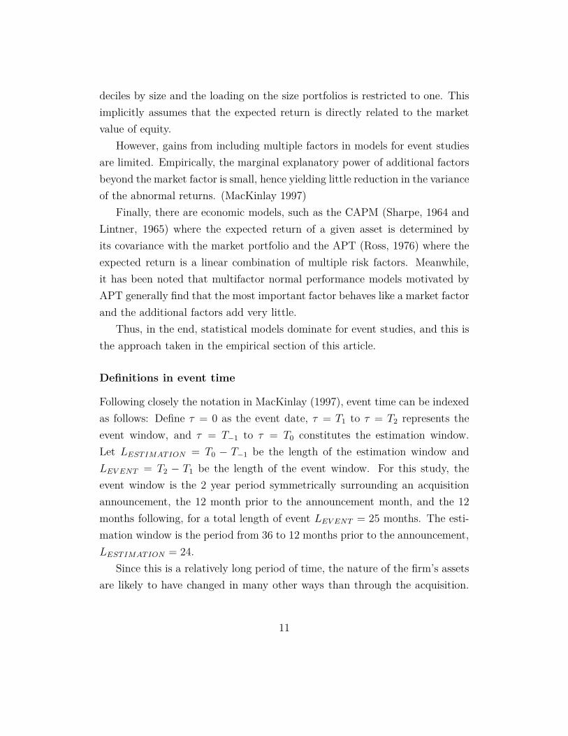
deciles by size and the loading on the size portfolios is restricted to one. This

implicitly assumes that the expected return is directly related to the market

value of equity.

However, gains from including multiple factors in models for event studies

are limited. Empirically, the marginal explanatory power of additional factors

beyond the market factor is small, hence yielding little reduction in the variance

of the abnormal returns. (MacKinlay 1997)

Finally, there are economic models, such as the CAPM (Sharpe, 1964 and

Lintner, 1965) where the expected return of a given asset is determined by

its covariance with the market portfolio and the APT (Ross, 1976) where the

expected return is a linear combination of multiple risk factors. Meanwhile,

it has been noted that multifactor normal performance models motivated by

APT generally find that the most important factor behaves like a market factor

and the additional factors add very little.

Thus, in the end, statistical models dominate for event studies, and this is

the approach taken in the empirical section of this article.

Definitions in event time

Following closely the notation in MacKinlay (1997), event time can be indexed

as follows: Define τ = 0 as the event date, τ = T1 to τ = T2 represents the

event window, and τ = T−1 to τ = T0 constitutes the estimation window.

Let LEST IMAT ION = T0 − T−1 be the length of the estimation window and

LEV ENT = T2 − T1 be the length of the event window. For this study, the

event window is the 2 year period symmetrically surrounding an acquisition

announcement, the 12 month prior to the announcement month, and the 12

months following, for a total length of event LEV ENT = 25 months. The esti-

mation window is the period from 36 to 12 months prior to the announcement,

LEST IMAT ION = 24.

Since this is a relatively long period of time, the nature of the firm’s assets

are likely to have changed in many other ways than through the acquisition.

11

Therefore, if we accept market efficiency in the sense that changes in a firm’s

value due to events are quickly and accurately incorporated into the price of

its stock, we should choose a shorter window. It is precisely because we want

to test the hypothesis that markets more slowly learn the true value of a firm

than the CEO, that we choose a longer window. There is a tradeoff between

measuring the effects specifically due to an acquisition precisely and capturing

long term effects, and by choosing such a long window, we clearly are giving

up some of this precision. To mitigate this, results will be controlled for ob-

servable factors that might influence a firm’s return aside from the acquisition

announcement. Further testing could reveal more about how returns in the

estimation window are correlated to returns in the event window in general,

and it would be ideal to control for this, but of necessity, errors are assumed

to be uncorrelated here.

Estimation of the Market Model and Statistical Properties

Given the market model parameter estimates of α and β from the procedure

outlined above, we can now examine the abnormal returns. Let ARiτ (τ=T1+1,...,T2)

be the sample of LEV ENT -length abnormal returns for firm i in the event win-

dow. Using the normal return measured above (by the market model) the

sample abnormal return is

ARiτ = Riτ − α̂i − β̂iRmτ

since we are using the market model:

Rit = αi + βiRmt + ǫit

We have ARiτ = ǫiτ . The abnormal return is simply the disturbance term

of the market model calculated on an out of sample basis. According to the

null hypothesis, conditional on the event-window market returns, the abnormal

returns will be jointly normally distributed with a zero conditional mean and

12

conditional variance σ2(ARiτ ) where

σ2(ARiτ ) = σ2ǫi

+1

L1

[

1 +(Rmτ − µ̂m)2

σ̂2m

]

This conditional variance of the abnormal return has two components: the

disturbance variance σ2ǫi

plus additional variance. The additional component

is due to the sampling error in αi and βi. This sampling error is common

for all the event window observations and leads to serial correlation in the

abnormal returns even if the true disturbances are independent through time.

Notice that as the length of the estimation window LEST IMAT ION increases, the

second term becomes smaller as the sampling error vanishes. To deal with this

in practice, we can choose an estimation window large enough that we assume

the contribution of the second term to the variance of abnormal returns is

zero. Nonetheless, this must be weighed against the representativeness of the

estimation window. As the estimation window includes more and more of the

past, the predictability of returns may diminish.

We can then formulate the null hypothesis:

• H0: the distribution of the sample abnormal return of a given observation

in the event window is

ARiτ ∼ N [0, σ2(ARiτ )].

Now we aggregate the abnormal returns, both through time, and across se-

curities. First consider time, then securities. We consider cumulative abnormal

return:

CARi(τ1,τ2) =τ2

∑

τ=τ1

ARiτ

Asymptotically (as LEST IMAT ION the length of the estimation window in-

creases to infinity) the variance of CARiis just

13

σ2i (τ1, τ2) = (τ2 − τ1 + 1)σ2

ǫi

Which is just the number of days in the event window multiplied by the

variance of returns, and can be used for large enough values of LEV ENT . If

it is not large enough, as in this case, (LEV ENT = 5) we need to add adjust-

ments: 1L1

[

1 + (Rmτ −µ̂m)2

σ̂2m

]

and another related term for serial covariance of the

abnormal return.

Under H0 we now have the distribution of the cumulative abnormal return

as

CARi(τ1,τ2) ∼ N (0, σ2i (τ1, τ2))

Using the null distributions of the abnormal return and CAR, we can conduct

tests of the null hypothesis. An issue that will arise is clustering, in the form

of overlap of the event windows of included securities. But if we assume no

overlap along with the above distributional assumptions, then the AR and

CAR will be independent across securities. We can take a simple average

ARτ of the ARs from all events to aggregate. The variance of ARτ , for large

LEV ENT is just

V ar(ARτ ) =1

N2

∑

σ2ǫi

.

Then we compute the cumulative abnormal returns for any event window

length, and their variance:

CARτ (τ1, τ2) =τ2

∑

τ=τ1

ARτ ,

V ar(CARτ (τ1, τ2)) =τ2

∑

τ=τ1

(ARτ ).

14

Or we could form the CAR’s by security and then aggregate through time,

which is equivalent. The assumption that the event windows of the N securities

don’t overlap is needed to set the covariance terms to 0. To make inferences

about the cumulative abnormal returns, we use

CARτ (τ1, τ2) ∼ N [0, (V ar(CARτ (τ1, τ2))]

to test the null hypothesis that the abnormal returns are zero. We can test

the null hypothesis using

θ1 =CARτ (τ1, τ2)

√

V ar(CARτ (τ1, τ2))∼ N (0, 1)

which is asymptotic with respect to the number of securities N and the length

of estimation window L1.

Though not done here, a common modification to this is to standardize

each abnormal return using an estimator of its standard deviation; for some

alternatives, such modifications can lead to more powerful tests. Without

having explored this approach at this stage.

Abnormal Returns in the Aggregate

In the previous section, we were interested in testing the null hypothesis that

for a given firm, an event has no impact on the distribution of returns. Now we

modify it. The new hypothesis only focuses on the mean of the distribution.

Using the cross section of CARs to estimate the variance of the CAR of a given

security, to allow for a change in variance from the estimation window to the

event window. This way we can test for a mean effect without imposing the

estimation window variance, which may well be smaller than the event window

one.

15

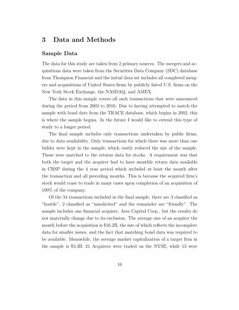
3 Data and Methods

Sample Data

The data for this study are taken from 2 primary sources. The mergers and ac-

quisitions data were taken from the Securities Data Company (SDC) database

from Thompson Financial and the initial data set includes all completed merg-

ers and acquisitions of United States firms by publicly listed U.S. firms on the

New York Stock Exchange, the NASDAQ, and AMEX.

The data in this sample covers all such transactions that were announced

during the period from 2002 to 2010. Due to having attempted to match the

sample with bond date from the TRACE database, which begins in 2002, this

is where the sample begins. In the future I would like to extend this type of

study to a longer period.

The final sample includes only transactions undertaken by public firms,

due to data availability. Only transactions for which there was more than one

bidder were kept in the sample, which vastly reduced the size of the sample.

These were matched to the returns data for stocks. A requirement was that

both the target and the acquirer had to have monthly return data available

in CRSP during the 4 year period which included at least the month after

the transaction and all preceding months. This is because the acquired firm’s

stock would cease to trade in many cases upon completion of an acquisition of

100% of the company.

Of the 34 transactions included in the final sample, there are 3 classified as

“hostile”, 2 classified as “unsolicited” and the remainder are “friendly”. The

sample includes one financial acquirer, Ares Capital Corp., but the results do

not materially change due to its exclusion. The average size of an acquirer the

month before the acquisition is $16.2B, the size of which reflects the incomplete

data for smaller issues, and the fact that matching bond data was required to

be available. Meanwhile, the average market capitalization of a target firm in

the sample is $3.3B. 21 Acquirers were traded on the NYSE, while 13 were

16

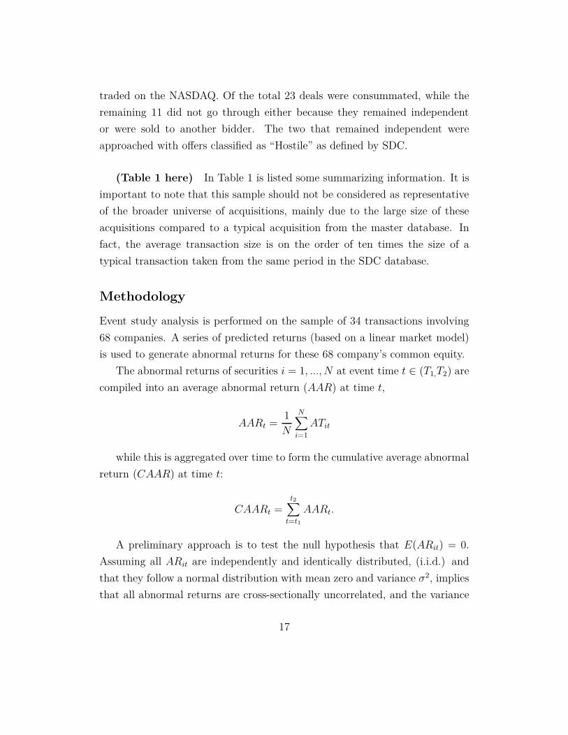
traded on the NASDAQ. Of the total 23 deals were consummated, while the

remaining 11 did not go through either because they remained independent

or were sold to another bidder. The two that remained independent were

approached with offers classified as “Hostile” as defined by SDC.

(Table 1 here) In Table 1 is listed some summarizing information. It is

important to note that this sample should not be considered as representative

of the broader universe of acquisitions, mainly due to the large size of these

acquisitions compared to a typical acquisition from the master database. In

fact, the average transaction size is on the order of ten times the size of a

typical transaction taken from the same period in the SDC database.

Methodology

Event study analysis is performed on the sample of 34 transactions involving

68 companies. A series of predicted returns (based on a linear market model)

is used to generate abnormal returns for these 68 company’s common equity.

The abnormal returns of securities i = 1, ..., N at event time t ∈ (T1,T2) are

compiled into an average abnormal return (AAR) at time t,

AARt =1

N

N∑

i=1

ATit

while this is aggregated over time to form the cumulative average abnormal

return (CAAR) at time t:

CAARt =t2

∑

t=t1

AARt.

A preliminary approach is to test the null hypothesis that E(ARit) = 0.

Assuming all ARit are independently and identically distributed, (i.i.d.) and

that they follow a normal distribution with mean zero and variance σ2, implies

that all abnormal returns are cross-sectionally uncorrelated, and the variance

17

of AARt ∼ N (0, σ2

N).

Using the cross-sectional variance of the time-t abnormal returns as an

estimator for σ2, σ̂2 , yields the test statistic

T =√

N

(

AARt

σ̂2

)

∼ tN−1

However, the normality assumption is in practice violated. Asymptotically

however, this statistic is distributed ∼ N (0, 1). With a sample size of 34, this

study is a little on the small side to assume this asymptotic distribution. We

would not be surprised to find somewhat different results with a much larger

sample.

The other assumption is also quite strong, that the ARit are i.i.d. Thus, we

will use a standardized abnormal return to help account for heteroskedasticity

between firms. Taking the firm i average return over the estimation period

ARi and firm i estimated standard deviation σ̂i yields a standardized abnor-

mal return (SAR). The cross-sectional average of the standardized abnormal

returns at time t can then be aggregated across time to give cumulative average

abnormal returns. The test statistic for this is

Z =√

N

(

1

N

) N∑

i=1

ARit

σ̂i

=1√N

N∑

i=1

SARit,

which asymptotically follows a normal distribution. The same statistic

is computed for cumulative abnormal returns (CAR) rather than abnormal

returns, and the results are reported in the next section.

4 Results

Let us begin with a caveat. Even though some of the results may be strik-

ing, and do lend evidence that supports the “market timing” hypothesis, they

are based on the small minority of cases where there is competition between

bidders. If it is true that M&A activity is driven by managers of overvalued

18

companies trying to essentially issue overpriced equity, we could imagine the

following scenario. Suppose there is an industry specific bubble, for example

the tech bubble of the 1990s. If managers of overpriced tech firms had all

been trying to buy firms with their overpriced stock at once, if we analyzed

this sample, we might expect to see evidence that indeed companies that per-

formed better were those who had bought other firm “on the cheap”, because

they would have done even worse otherwise (like their industry peers who did

not buy up other companies). But then there would be a correlation between

there being a competing bid on a given merger, and the likelihood that that

merger is being done under “bubbly” conditions where the acquiring firm’s

stock is overpriced.

Thus, even if we observe that acquiring firms do much better than firms

that miss out on the opportunity to acquire, these results may not be as strong

as for firms that don’t face competing bidders. On the other hand, a firm that

has no competing bidders has more bargaining power, and thus, conditional

on completing an acquisition, may do better than a firm that also completed

its acquisition, but had to outbid a competitor. Therefore, the generalizability

to other firms that don’t face competition is ambiguous.

Individual time-series

Keeping this type of scenario in mind the results of individual regressions

are presented in table 2. We see that within individual acquiring firms, only

2 out of 13 are positive and significant, while 11 are significantly negative.

Roughly the same proportion of these transactions are between firms in the

same industry (as classified by their two-digit primary SIC code) as in the

whole sample. The same is true for whether the deal was consummated. One

of these significantly negative deals occurs in 2003, 2007 and 2008. Two of these

significant deals occur in each of 2002, 2004, and 2006. In 2005, 3 significantly

negative deals occurred. The only significantly positive abnormal return in

the sample was an uncompleted deal that occurred in 2005, when Commscope

19

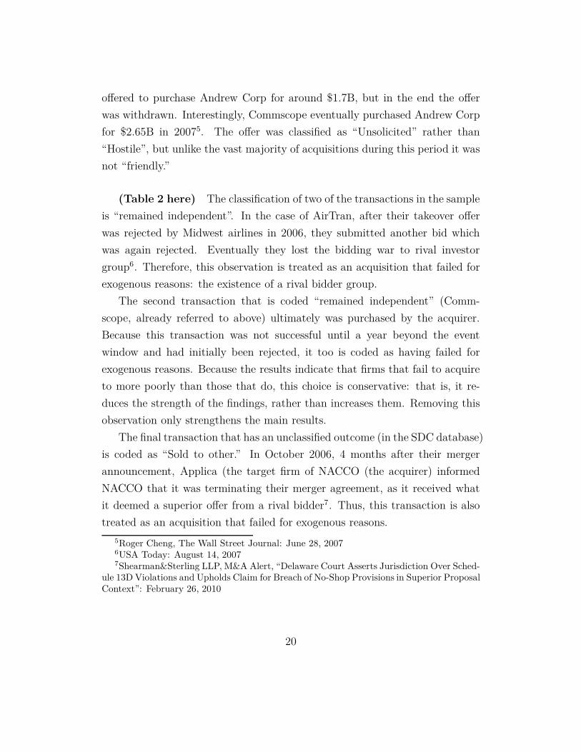
offered to purchase Andrew Corp for around $1.7B, but in the end the offer

was withdrawn. Interestingly, Commscope eventually purchased Andrew Corp

for $2.65B in 20075. The offer was classified as “Unsolicited” rather than

“Hostile”, but unlike the vast majority of acquisitions during this period it was

not “friendly.”

(Table 2 here) The classification of two of the transactions in the sample

is “remained independent”. In the case of AirTran, after their takeover offer

was rejected by Midwest airlines in 2006, they submitted another bid which

was again rejected. Eventually they lost the bidding war to rival investor

group6. Therefore, this observation is treated as an acquisition that failed for

exogenous reasons: the existence of a rival bidder group.

The second transaction that is coded “remained independent” (Comm-

scope, already referred to above) ultimately was purchased by the acquirer.

Because this transaction was not successful until a year beyond the event

window and had initially been rejected, it too is coded as having failed for

exogenous reasons. Because the results indicate that firms that fail to acquire

to more poorly than those that do, this choice is conservative: that is, it re-

duces the strength of the findings, rather than increases them. Removing this

observation only strengthens the main results.

The final transaction that has an unclassified outcome (in the SDC database)

is coded as “Sold to other.” In October 2006, 4 months after their merger

announcement, Applica (the target firm of NACCO (the acquirer) informed

NACCO that it was terminating their merger agreement, as it received what

it deemed a superior offer from a rival bidder7. Thus, this transaction is also

treated as an acquisition that failed for exogenous reasons.

5Roger Cheng, The Wall Street Journal: June 28, 20076USA Today: August 14, 20077Shearman&Sterling LLP, M&A Alert, “Delaware Court Asserts Jurisdiction Over Sched-

ule 13D Violations and Upholds Claim for Breach of No-Shop Provisions in Superior ProposalContext”: February 26, 2010

20

Cross-section

To demonstrate the prevailing patterns found in the sample we can create

hypothetical portfolios of acquirer stocks and target stocks. The graphical

representations generated from this procedure will mirror the regression to

follow, with the difference that the graphs will equally weight the abnormal

returns contributed from each stock, whereas the regression will use a weighting

procedure to standardize individual securities by the standard deviations of

their returns to lower the contribution of high-variance firms to the results.

At the cross-sectional level, the abnormal returns of each individual stock

can be labeled with an event time, generating a cross-section of returns in each

observation of event time. For expositional purposes, we can represent this in

the following matrix:

AR1,T1........ ARN,T1

| ... |AR1,−1 ... ARN,−1

AR1,0 ... ARN,0

AR1,1 ... ARN,1

| ... |AR1,T2

........ ARN,T2

.

The columns of this (T2 − T1) by N matrix represent all the returns of

a given security, while the rows represent a cross-section in event time of all

the time t returns of the N securities. For the graphs that follow, the data

point for month i in event time is generated from the average of the returns

corresponding to that month, exactly as AARt is defined in the methodology

section, and for each month the holding-period return is computed as if an

investor were holding the hypothetical portfolio and reinvesting the proceeds.

In figure 1, we see the performance of all the acquirers and all the targets in

the sample.

21

(Figure 1 here) Figure 1 shows the typical pattern that has been ob-

served in the literature of target shareholders reaping gains from takeovers. The

acquirers in this sample perform worse than acquirers do in typical event stud-

ies, under-performing by 30 percent relative to their market-model predicted

returns. The average market model predicted return for acquirers works out to

12% on an annual basis, which seems like it could be a bit optimistic. Here we

note that for longer time periods it would perhaps be an improvement to use

a multifactor model for generating the predicted returns, such as the Fama-

French (1993) multifactor model referenced earlier. Still, for the acquirers to

have generated positive abnormal returns (given the returns that they actu-

ally did produce), the return prediction model would have to have predicted

significantly negative returns, so on average acquiring firms are losing value

here.

(Figure 2 here) Figure 2 shows the acquirer’s returns that were repre-

sented by downward sloping blue line in figure 1, but divided into two sub-

samples. Sorting the sample into firms that were successful in their acquisition

and those that weren’t yields this striking pattern. The 21 acquirers who ended

up successfully acquiring their targets didn’t display returns significantly dif-

ferent than the market model predicted return. The 13 firms that did not end

up completing their acquisitions are the firms that lost the most value. Of note

is that the firms began to lose value long before their transactions fell through,

or were even announced. It is therefore likely that there is an endogeneity issue

in the sample.

Though the sample was selected to identify firms whose acquisitions failed

due to the success of a rival bidder, it seems likely that target firm boards,

in choosing between suitors, are not as keen to sell to a firm whose value

has recently significantly decreased. In addition, it is possible that bidding

firms become financially constrained as their value falls, perhaps running to

bondholder covenant constraints that force them to withdraw their offers. Even

though in this sample all the failed acquisition attempts are coded as being

22

due to a rival bidder succeeding, it is impossible to be rule out that the decline

in the acquirer’s value itself didn’t drive the fact that they weren’t successful

in making their acquisition.

(Table 3 here) These results are testing using the null hypothesis that

cumulative abnormal returns of the sample are 0. Using the standardized cu-

mulative abnormal returns, the null hypothesis that they equal 0 is tested for

several sub-samples, including the sub-sample illustrated in figure 2. In addi-

tion, this is further divided into those transactions for which the sole medium

of exchange was cash, and those for which the financing was a mixture of

stock and cash or pure stock. This division shows that the aggregate result

is driven by the sub-sample of transactions that were canceled and involved

stock. Similar to the findings of Savor and Lu (2009), acquirers whose deals

were canceled appear to do worse than those whose deals were successful. The

fact that acquirers who purchase with their stock do worse also lends cred

Questions for Future Research

The question of whether managerial decisions are in the interests are sharehold-

ers can be difficult to address. As was pointed out in Myers and Majluf (1984)

and Shleifer and Vishny (2003), managers may well to try to issue equity when

it is “expensive” relative to its value and engage in inefficient transactions.

Using the small data-set employed in this study it is impossible to accurately

asset how target stockholders fare following a transaction announcement, since

in several cases the timing is ambiguous or data is lacking.

(Figure 3 here) Figure 3 shows the same information as Figure 2 but

for the set of target firms. The puzzling aspect of figure 3 is that targets

for whom acquisitions are ultimately completed appear to do quite poorly,

achieving comparable gains in the months leading up to and including the

acquisition month, but then retreating back to their former valuations. This

23

appears to driven by the fact that not all the acquisitions involved taking over

100 percent of the shares, and thus the shares continued to trade. Perhaps

investors did not see a fundamental change in the value of the company due to

its controlling shareholder changing. To address this question properly would

require paying a great deal of attention to the timing of the events subsequent

to an acquisition announcement, such as the actual execution of the transaction

or the date of withdrawal. Since these events all occur a different number of

periods into the future for different firms, it can complicate the procedure, and

would require a more sophisticated analysis.

(Figure 4 here) Figure 4 overlays acquirer and target firm returns, for

the set of transactions where the consideration was cash only separately from

the set of transactions that involved stock only of a combination of cash and

stock. The interesting finding is that targets purchased for cash do much better

than those purchased for equity. Again, If the equity being using is overvalued,

we would expect a kind of “exchange rate parity” not to hold. That is, if an

overvalued firm is using its stock to purchase the assets of another firm, once a

large block of the acquirer’s stock is in the hands of of the target shareholders,

they find little use for it; it cannot be converted at the same exchange rate for

cash at which it was trading prior to the acquisition.

It would also be interesting to examine the returns of target and acquirer

bonds over the same time period. Whether risk shifting/asset substitution

occurs as a part of M&A is a question that has perhaps not been studied in

depth, and to examine the returns of other asset classes and how they co-move

with equity returns is a topic for ongoing research along the lines of what is

done in papers like this.

5 Conclusions

Using a small but recent data-set, this study provides evidence that firms that

fail to complete acquisitions suffer lower returns than those that successfully

24

acquire. If this finding was confirmed for a more comprehensive data-set, it

would represent solid evidence that managers of acquiring firms are acting in

the interest of their shareholders, and provide a counterpoint to theories of

managerial behavior that point to empire-building and hubris.

Additionally, these results were mainly driven by firms that used their stock

as currency in the transaction, which is suggestive that managers may indeed be

timing the market by issuing equity when it is expensive. This result, if found

to be generally true, implies the informational relationship between market and

“insider” managers is indeed complex, and that markets are not strong-form

efficient. The pattern of returns taking on the order of 2 years to adjust to

their factor-predicted levels is indicative that markets incorporate information

more slowly than would be captured by a very short term (i.e. 5 days) event

study, and calls into question the long-run validity of the conclusions of these

studies.

While the results of this study must be considered with caution due to the

small sample and limited data and the consequent lack of ability to control for,

for example, industry fixed effects, book-to-market and leverage (due to lack

of accounting data in the sample) there are a number of promising directions

for research highlighted by this attempt. With sufficient data, along the lines

of Savor and Lu (2009), one could analyze the returns of both debt and equity

claims of firms that were identified to have failed to complete a takeover of a

company for exogenously reasons, to gain a richer picture of the impact of a

specific managerial decision on firm performance.

Indeed, two very important general facts have been highlighted in this

paper. (1) If we are to study the impact of corporate decisions on the price

of a stock, it is important to look at longer timeframes. In event studies,

one ought not to accept the hypothesis of market efficiency as being true,

and use this as a justification for using only a short interval. If persistent

patterns are found at longer timeframes, this means that either a significant

exogenous factor is not being controlled for, or that the original presumption

of market efficiency is false. (2) Due to the inseperability of the determination

25

of managerial decisions and firm value, it is necessary to try to measure the

impact of the former on the latter using a procedure that is robust to this

endogeneity and feedback effects. In this case, a “placebo” sample was created

of firms whose managers intended to take the action whose merits we wished

to test; the reason they couldn’t take the action was exogenous - another firm

preempted them.

To allow the possibility of firm value influencing managerial actions as

opposed to only the other way around is to invalidate the traditional approach

of event studies. But it is an eminently sensible notion, and it should be

tested. In this paper, an attempt has been made to show a way of doing this,

and I believe the fact that the results differ so significantly from the results of

applying the traditional method which ignores this warrants significant further

investigation.

References

[1] A. Craig MacKinlay, (1997), Event Studies in Economics and Fi-

nance. Journal of Economic Literature Vol. 35, No. 1 pp. 13-39

[2] Andrade, G., Mitchell, M., Stafford, E., (2001), New evidence

and perspectives on mergers. Journal of Economic Perspectives

15, 103–120.

[3] Billett, M. T., King, T.-H. D. and Mauer, D. C. (2004), Bond-

holder Wealth Effects in Mergers and Acquisitions: New Evidence

from the 1980s and 1990s. The Journal of Finance, 59: 107–135

[4] Bernard, Victor L. (1987), Cross-Sectional Dependence and Prob-

lems in Inference in Market-Based Accounting Research. Journal

of Accounting Research Vol. 25, No. 1, pp. 1-48

[5] Bradley, Michael and Sundaram, Anant K., (2006) working paper.

Acquisitions and Performance: A Re-Assessment of the Evidence

26

[6] Brown, Stephen J. and Warner, Jerold B., (1980), Measuring se-

curity price performance, Journal of Financial Economics, 8, issue

3, p. 205-258

[7] Brown, Stephen J. and Jerold B. Warner, (1985), Using daily

stock returns : The case of event studies. Journal of Financial

Economics Volume 14, Issue 1, Pages 3-31

[8] Fama, Eugene F.; French, Kenneth R. (1993). "Common Risk

Factors in the Returns on Stocks and Bonds". Journal of Financial

Economics

[9] Ferris, Kenneth R. and Nikhil P. Varaiya. (1987), Overpaying in

Corporate Takeovers: The Winner’s Curse. Financial Analysts

Journal Vol. 43, No. 3, pp. 64-70

[10] Hansen, Robert G. and John R. Lott (1996), Externalities

and Corporate Objectives in a World with Diversified Share-

holder/Consumers. Journal of Financial and Quantitative Analy-

sis, 31, pp 43-68

[11] Jensen, M.C. (1986) Agency costs of free cash flow: Corporate

finance and takeovers. American Economic Review, 76(2), 323-

329.

[12] Jensen, M. C. (2005), Agency Costs of Overvalued Equity. Finan-

cial Management, 34: 5–19.

[13] Moeller, Schlingemann, and Stulz (2005), Wealth Destruction on

a Massive Scale? A Study of Acquiring-Firm Returns in the Re-

cent Merger Wave. The Journal of Finance, 60: 757–782.

[14] Myers Stewart C. & Nicholas S. Majluf, (1984), Corporate Fi-

nancing and Investment Decisions When Firms Have Information

27

That Investors Do Not Have, NBER Working Papers 1396, Na-

tional Bureau of Economic Research, Inc.

[15] Myerson (1981). Optimal auction design. Mathematics of Opera-

tions Research, 6(1), 58–73.

[16] Lintner, John, (1965), The Valuation of Risk Assets and the Selec-

tion of Risky Investments in Stock Portfolios and Capital Budgets

The Review of Economics and Statistics Vol. 47, No. 1 pp. 13-37

[17] Loughran, Tim and Anand M. Vijh, (1997) Do Long-Term Share-

holders Benefit From Corporate Acquisitions? The Journal of

Finance Vol. 52, No. 5 (Dec., 1997), pp. 1765-1790

[18] Raghavendra Rau P., Vermaelen T. (1998) Glamour, value and

the post-acquisition performance of acquiring firms, Journal of

Financial Economics, Volume 49, Number 2, 1 August 1998 , pp.

223-253(31)

[19] Ross, S. 1976. The arbitrage theory of capital asset pricing. Jour-

nal of Economic Theory 13, 341–60

[20] Savor, P. G. and Lu, Q. (2009), Do Stock Mergers Create Value

for Acquirers?. The Journal of Finance, 64: 1061–1097.

[21] Sharpe, William F. (1964), Capital Asset Prices: A Theory of

Market Equilibrium under Conditions of Risk The Journal of Fi-

nance Vol. 19, No. 3 pp. 425-442

[22] Shearman&Sterling LLP, M&A Alert, “Delaware Court Asserts

Jurisdiction Over Schedule 13D Violations and Upholds Claim

for Breach of No-Shop Provisions in Superior Proposal Context”:

February 26, 2010

[23] Shleifer, Andrei & Vishny, Robert W. (2003), Stock market driven

acquisitions. Journal of Financial Economics, 70, 295- 311.

28

[24] Thaler, Richard H. (1988). Anomalies: The Winner’s Curse. The

Journal of Economic Perspectives Vol. 2, No. 1 (Winter, 1988),

pp. 191-202

[25] Vickrey, W. (1961). Counterspeculation, auctions, and competi-

tive sealed tenders. The Journal of Finance, 16(1), 8–37

29