are ideas getting harder to find? - review of economic ... · are ideas getting harder to find? 3...
TRANSCRIPT
Are Ideas Getting Harder to Find?
Nicholas Bloom Charles I. Jones
Stanford University and NBER Stanford University and NBER
John Van Reenen Michael Webb∗
MIT and NBER Stanford University
January 4, 2017 — Version 0.6
Preliminary and Incomplete
Abstract
In many growth models, economic growth arises from people creating ideas,
and the long-run growth rate is the product of two terms: the effective number of
researchers and the research productivity of these people. We present a wide range
of evidence from various industries, products, and firms showing that research
effort is rising substantially while research productivity is declining sharply. A good
example is Moore’s Law. The number of researchers required today to achieve the
famous doubling every two years of the density of computer chips is more than
75 times larger than the number required in the early 1970s. Across a broad range
of case studies at various levels of (dis)aggregation, we find that ideas — and in
particular the exponential growth they imply — are getting harder and harder to
find. Exponential growth results from the large increases in research effort that
offset its declining productivity.
∗We are grateful to Daron Acemoglu, Ufuk Akcigit, Michele Boldrin, Pete Klenow, Peter Kruse-Andersen, Rachel Ngai, Pietro Peretto, Unni Pillai, John Seater, Chris Tonetti, and participants at the CEPRMacroeconomics and Growth Conference, the Rimini Conference on Economics and Finance, and theNBER Macro across Time and Space conference for helpful comments and to Wallace Huffman, KeithFuglie, and Greg Traxler for kindly providing data and insight on agricultural R&D expenditures. TheEuropean Research Council and ESRC have provided financial support.

2 BLOOM, JONES, VAN REENEN, AND WEBB
1. Introduction
The basic insight of this paper can be explained with a simple equation, highlighting a
stylized view of economic growth that emerges from idea-based growth models:
Economicgrowth
= Idea TFP × Number ofresearchers
e.g. 2% or 5% ↓(falling) ↑(rising)
Economic growth arises from people creating ideas, and the long-run growth rate is the
product of two terms: the effective number of researchers and the research productivity
of these people (“idea TFP”). We present a wide range of empirical evidence showing
that in many different contexts and at various levels of disaggregation, research effort
is rising substantially, while research productivity is declining sharply. Steady growth,
when it occurs, results from the offsetting of these two trends.
Perhaps the best example of this finding comes from studying Moore’s Law, one of
the key drivers of economic growth in recent decades. This “law” refers to the empirical
regularity that the number of transistors packed onto a computer chip doubles approx-
imately every two years. Such doubling corresponds to a constant exponential growth
rate of around 35% per year, a rate that has been remarkably steady for nearly half a
century. As we show in detail below, this growth has been achieved by putting an ever-
growing number of researchers to work on pushing Moore’s Law forward. In particular,
the number of researchers required to achieve the doubling of chip density today is
more than 75 times larger than the number required in the early 1970s. At least as far as
semiconductors are concerned, ideas are getting harder and harder to find. Idea TFP in
this case is declining sharply, at a rate that averages about 10% per year.
We document qualitatively similar results essentially no matter where we look in
the U.S. economy. We consider detailed microeconomic evidence on idea production
functions, focusing on places where we can get the best measures of both the output of
ideas and the inputs used to produce them. In addition to Moore’s Law, our case stud-
ies include agricultural productivity (corn, soybeans, cotton, and wheat) and medical
innovations. Idea TFP for seed yields declines at about 5% per year. We find a similar
rate of decline when studying the mortality improvements associated with all cancers
and with breast cancer. Finally, we examine firm-level data from Compustat to provide

ARE IDEAS GETTING HARDER TO FIND? 3
another perspective on idea TFP. While the data quality from this sample is not as good
as for our industry case studies, the latter suffer from possibly not being representative.
We find substantial heterogeneity across firms, but idea TFP is declining in more than
85% of the firms in our sample. Averaging across firms, idea TFP declines at a rate of
12% per year.
Perhaps idea TFP is declining sharply within every particular case that we look at
and yet not declining for the economy as a whole. While existing varieties run into
diminishing returns, perhaps new varieties are always being invented to stave this off.
We consider this possibility by taking it to the extreme. Suppose each variety has a
productivity that cannot be improved at all, and instead aggregate growth proceeds
entirely by inventing new varieties. To examine this case, we consider idea TFP for
the economy as a whole. We once again find that it is declining sharply: aggregate
growth rates are relatively stable over time,1 while the number of researchers has risen
enormously. In fact, this is simply another way of looking at the original point of Jones
(1995), and for this reason, we present this application first to illustrate our methodol-
ogy. We find that idea TFP for the aggregate U.S. economy has declined by a factor of
48 since the 1930s, an average decrease of more than 5% per year.
Despite these large declines in idea TFP, relatively stable exponential growth is com-
mon in the cases we study (and in the aggregate U.S. economy). How is this possible?
Looking back at the equation that began the introduction, declines in idea TFP must
be offset by increased research effort, and this is indeed what we find. Moreover, we
suggest at the end of the paper that the rapid declines in idea TFP that we see in semi-
conductors, for example, might be precisely due to the fact that research effort is rising
so sharply. Because it gets harder to find new ideas as research progresses, a sustained
and massive expansion of research like we see in semiconductors (for example, because
of the “general purpose technology” nature of information technology), may lead to a
substantial downward trend in idea TFP.
Others have also provided evidence suggesting that ideas may be getting harder to
1There is a debate over whether the slower rates of growth over the last decade are a temporaryphenomenon due to the global financial crisis, or a sign of slowing technological progress. Gordon (2016)argues that the strong US productivity growth between 1996 and 2004 was a temporary blip and thatproductivity growth will, at best, return to the lower growth rates of 1973–1996. Although we do not needto take a stance on this, note that if frontier TFP growth really has slowed down, this only strengthens ourargument.

4 BLOOM, JONES, VAN REENEN, AND WEBB
find over time. Griliches (1994) provides a summary of the earlier literature exploring
the decline in patents per dollar of research spending. Gordon (2016) reports extensive
new historical evidence from throughout the 19th and 20th centuries. Cowen (2011)
synthesizes earlier work to explicitly make the case. (Ben) Jones (2009) documents
a rise in the age at which inventors first patent and a general increase in the size of
research teams, arguing that over time more and more learning is required just to get
to the point where researchers are capable of pushing the frontier forward. We see our
evidence as complementary to these earlier studies.
The remainder of the paper is organized as follows. Section 2 lays out our con-
ceptual framework and presents the aggregate evidence on idea TFP to illustrate our
methodology. Section 3 places this framework in the context of growth theory and
suggests that applying the framework to micro data is crucial for understanding the
nature of economic growth. Sections 4 through 7 consider our applications to Moore’s
Law, agricultural yields, medical technologies, and Compustat firms. Section 8 then
revisits the implications of our findings for growth theory, and Section 9 concludes.
2. Idea TFP and Aggregate Evidence
2.1. The Conceptual Framework
An equation at the heart of many growth models is an idea production function taking
a particular form:AtAt
= αSt. (1)
Classic examples include Romer (1990) and Aghion and Howitt (1992), but many recent
papers follow this approach, including Aghion, Akcigit and Howitt (2014), Acemoglu
and Restrepo (2016), Akcigit, Celik and Greenwood (2016), and Jones and Kim (2014).
In the equation above, At/At is total factor productivity growth in the economy. The
variable St (think “scientists”) is some measure of research input, such as the number
of researchers. This equation then says that the growth rate of the economy — through
the production of new ideas — is proportional to the number of researchers.
Relating At/At to ideas runs into the familiar problem that ideas are hard to mea-
sure. Even as simple a question as “What are the units of ideas?” is troublesome. We

ARE IDEAS GETTING HARDER TO FIND? 5
follow much of the literature — including Aghion and Howitt (1992), Grossman and
Helpman (1991), and Kortum (1997) — and define ideas to be in units so that a constant
flow of new ideas leads to constant exponential growth in A. For example, each new
idea raises incomes by a constant percentage (on average), rather than by a certain
number of dollars. This is the standard approach in the quality ladder literature on
growth: ideas are proportional improvements in productivity. The patent statistics for
most of the 20th century are consistent with this view; indeed, this was a key piece of
evidence motivating Kortum (1997). This definition means that the left hand side of
equation (1) corresponds to the flow of new ideas.
We can now define the productivity of the idea production function, which we call
“idea TFP,” as the ratio of the output of ideas to the inputs used to make them:
Idea TFP :=At/AtSt
=# of new ideas
# of researchers. (2)
The null hypothesis tested in this paper comes from the relationship assumed in (1).
Substituting this equation into the definition of idea TFP, we see that (1) implies that
idea TFP equalsα— that is, idea TFP is constant over time. This is the standard hypoth-
esis in much of the growth literature. Under this null, a constant number of researchers
can generate constant exponential growth.
The reason this is such a common assumption is also easy to see in equation (1).
With constant idea TFP, a research subsidy that increases the number of researchers
permanently will permanently raise the growth rate of the economy. In other words
“constant idea TFP” and the fact that sustained research subsidies produce “perma-
nent growth effects” are equivalent statements.2 This clarifies a claim in the introduc-
tion: testing the null hypothesis of constant idea TFP is interesting in its own right
but also because it is informative about the kind of models that we use to study eco-
nomic growth. The finding that idea TFP is declining virtually everywhere we look
poses problems for a large class of endogenous growth models. Moreover, the way we
have defined ideas gives this concept economic relevance: exponential growth (e.g. in
2The careful reader may wonder about this statement in richer models — for example, lab equipmentmodels where research is measured in goods rather than in bodies or models with both horizontal andvertical dimensions to growth. These extensions will be incorporated below in such a way as to maintainthe equivalence between “constant idea TFP” and “permanent growth effects.”

6 BLOOM, JONES, VAN REENEN, AND WEBB
semiconductor density or seed yields or living standards) is getting harder to find.
2.2. Aggregate Evidence
The bulk of the evidence presented in this paper concerns the extent to which a con-
stant level of research effort can generate constant exponential growth within a rela-
tively narrow category, such as a firm or a seed type or Moore’s Law or a health condi-
tion. We provide consistent evidence that the historical answer to this question is no:
idea TFP is declining at a substantial rate in virtually every place we look.
This finding raises a natural question, however. What if there is sharply declin-
ing idea TFP within each product line, but the main way that growth proceeds is by
developing ever-better new product lines? First there was steam power, then electric
power, then the internal combustion engine, then the semiconductor, then gene edit-
ing, and so on. Maybe there is limited opportunity within each area for productivity
improvement and long-run growth occurs through the invention of entirely new areas.
Maybe idea TFP is declining within every product line, but still not declining for the
economy as a whole because we keep inventing new products. An analysis focused on
microeconomic case studies would never reveal this to be the case.
The answer to this concern turns out to be straightforward and is an excellent place
to begin. First, consider the extreme case where there is no possibility at all for produc-
tivity improvement in a product line and all productivity growth comes from adding
new product lines. Of course, this is just the original Romer (1990) model itself, and
to generate constant idea TFP in that case requires the equation we started the paper
with:AtAt
= αSt. (3)
In this interpretation,At represents the number of product varieties and St is the aggre-
gate number of researchers. Even with no ability to improve productivity within each
variety, a constant number of researchers can sustain exponential growth if the variety-
discovery function exhibits constant idea TFP.
This hypothesis, however, runs into an important well-known problem.3 For the
U.S. economy as a whole, exponential growth rates in GDP per person since 1870 or in
total factor productivity since the 1930s — which are related to the left side of equa-
3For example, see Jones (1995).
ARE IDEAS GETTING HARDER TO FIND? 7
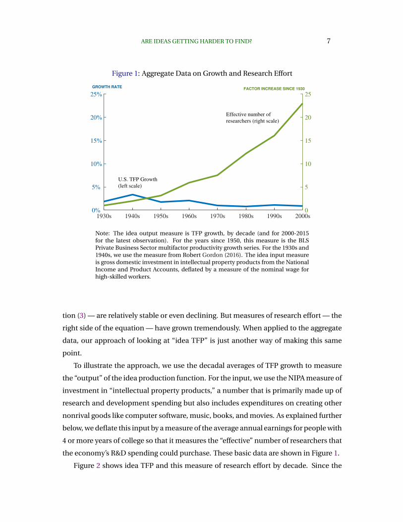
Figure 1: Aggregate Data on Growth and Research Effort
1930s 1940s 1950s 1960s 1970s 1980s 1990s 2000s0%
5%
10%
15%
20%
25%
U.S. TFP Growth
(left scale)
Effective number of
researchers (right scale)
GROWTH RATE
0
5
10
15
20
25FACTOR INCREASE SINCE 1930
Note: The idea output measure is TFP growth, by decade (and for 2000-2015for the latest observation). For the years since 1950, this measure is the BLSPrivate Business Sector multifactor productivity growth series. For the 1930s and1940s, we use the measure from Robert Gordon (2016). The idea input measureis gross domestic investment in intellectual property products from the NationalIncome and Product Accounts, deflated by a measure of the nominal wage forhigh-skilled workers.
tion (3) — are relatively stable or even declining. But measures of research effort — the
right side of the equation — have grown tremendously. When applied to the aggregate
data, our approach of looking at “idea TFP” is just another way of making this same
point.
To illustrate the approach, we use the decadal averages of TFP growth to measure
the “output” of the idea production function. For the input, we use the NIPA measure of
investment in “intellectual property products,” a number that is primarily made up of
research and development spending but also includes expenditures on creating other
nonrival goods like computer software, music, books, and movies. As explained further
below, we deflate this input by a measure of the average annual earnings for people with
4 or more years of college so that it measures the “effective” number of researchers that
the economy’s R&D spending could purchase. These basic data are shown in Figure 1.
Figure 2 shows idea TFP and this measure of research effort by decade. Since the

8 BLOOM, JONES, VAN REENEN, AND WEBB
Figure 2: Aggregate Evidence on Idea TFP
1930s 1940s 1950s 1960s 1970s 1980s 1990s 2000s 1/64
1/32
1/16
1/8
1/4
1/2
1
Idea TFP
(left scale)
Effective number of
researchers (right scale)
INDEX (1930=1)
1
2
4
8
16
32INDEX (1930=1)
Note: Idea TFP is the ratio of Idea Output, measured as TFP growth, to researcheffort. See notes to Figure 1. Both idea TFP and research effort are normalized tothe value of 1 in the 1930s.
1930s, research effort has risen by a factor of 23 — an average growth rate of 4.3 percent
per year. Idea TFP has fallen by an even larger amount — by a factor of 48 (or at an
average growth rate of -5.3 percent per year). By construction, a factor of 23 of this
decline is due to the rise in research effort and so only about a factor of 2 is due to the
well-known decline in TFP growth.
The “new economy” of the 1990s exhibited a bounceback of TFP growth that was
roughly of the same factor as the increase in research in that decade, resulting in flat
idea TFP between the 1980s and 1990s. But the overall trend is clear. For example,
between the 1960s and the 2000s, idea TFP fell by a factor of 9.2. And between the 1980s
and the 2000s, it fell by a factor of 1.7, with the entire amount due to rising research
effort.
This aggregate evidence could be improved on in many ways. One might question
the TFP growth numbers — how much of TFP growth is due to innovation versus real-
location or declines in misallocation? One might seek to include international research
in the input measure. But reasonable variations along these lines would not change the
basic point of Figure 2: a model in which economic growth arises from the discovery of

ARE IDEAS GETTING HARDER TO FIND? 9
newer and better varieties with limited possibilities for productivity growth within each
variety exhibits sharply-declining idea TFP. If one wishes to maintain the hypothesis of
constant idea TFP, one must look elsewhere. It is for this reason that the literature —
and this paper — turns to the micro side of economic growth.
3. Refining the Conceptual Framework
In this section, we further develop the conceptual framework introduced in the previ-
ous section. First, we explain why the aggregate evidence just presented can be mis-
leading, motivating our focus on micro data. Second, we consider the measurement
of idea TFP when the input to research is R&D expenditures (i.e. “goods”) rather than
just bodies or researchers (i.e. “time”). Finally, we discuss various extensions to our
calculation of idea TFP.
3.1. The Importance of Micro Data
The null hypothesis that idea TFP is constant over time is attractive conceptually in
that it leads to models in which changes in policies related to research can permanently
affect the growth rate of the economy. Several papers, then, have proposed alternative
models in which the calculations using aggregate data can be misleading about idea
TFP. The insight of Dinopoulos and Thompson (1998), Peretto (1998), Young (1998), and
Howitt (1999) is that the aggregate evidence may be masking important heterogeneity,
and that idea TFP may nevertheless be constant for a significant portion of the econ-
omy. Perhaps the idea production function for individual products shows constant idea
TFP. The aggregate numbers may simply capture the fact that every time the economy
gets larger we add more products, so the aggregate calculation mismeasures idea TFP.4
To see the essence of the argument, suppose that the economy produces Nt dif-
ferent products, and each of these products is associated with some quality level Ait.
Innovation can lead the quality of each product to rise over time according to an idea
production function,AitAit
= αSit. (4)
4This line of research has been further explored by Aghion and Howitt (1998), Li (2000), Laincz andPeretto (2006), Dinopoulos and Syropoulos (2007), Ha and Howitt (2007), Kruse-Andersen (2016), andPeretto (2016a; 2016b).

10 BLOOM, JONES, VAN REENEN, AND WEBB
Here, Sit is the number of scientists devoted to improving the quality of good i, and in
a symmetric case, we might have Sit = StNt
. The key is that the aggregate number of
scientists St can be growing, but perhaps the number per product St/Nt is not growing.
This can occur in equilibrium if the number of products itself grows endogenously
at the right rate. In this case, the aggregate evidence discussed earlier would not tell
us anything about the idea production functions associated with the quality improve-
ments of each variety. Instead, aggregation masks the true constancy of idea TFP at the
micro level.
This insight provides one of the key motivations for the present paper: to study the
idea production function at the micro level. That is, we study equation (4) directly and
consider idea TFP for individual products:
Idea TFP: iTFPit :=Ait/AitSit
. (5)
By considering micro evidence, we can directly test the key hypothesis underlying a
large portion of endogenous growth theory.
3.2. “Lab Equipment” Specifications
In many applications, the input that we measure is R&D expenditures rather than the
number of researchers. In fact, one could make the case that this is a more desirable
measure, in that it weights the various research inputs according to their relative prices:
if expanding research involves employing people of lower talent, this will be properly
measured by R&D spending. When the only input into ideas is researchers, then de-
flating R&D expenditures by an average wage will appropriately recover the effective
quantity of researchers. In practice, R&D expenditures also typically involve spending
on capital goods and materials. As explained next, deflating by the nominal wage to
get an “effective number of researchers” that this research spending could purchase
remains a good way to proceed.
In the growth literature, these specifications are called “lab equipment” models,
because implicitly both capital and labor are used as inputs to produce ideas. In lab
equipment models, the endogenous growth case occurs when the idea production func-

ARE IDEAS GETTING HARDER TO FIND? 11
tion takes the form
At = αRt, (6)
where Rt is measured in units of a final output good. For the moment, we discuss this
issue in the context of a single-good economy; in the next section, we explain how the
analysis extends to the case of multiple products.
To see why equation (6) delivers endogenous growth, it is necessary to specify the
economic environment more fully. First, suppose there is a final output good that is
produced with a standard Cobb-Douglas production function:
Yt = Kθt (AtL)1−θ. (7)
Next, the resource constraint for this economy is
Yt = Ct + It +Rt (8)
That is, final output is used for consumption, investment in physical capital, or re-
search.
We can now combine these three equations to get the endogenous growth result.
First, notice that dividing both sides of the production function for final output by Y θ
and rearranging yields
Yt =
(Kt
Yt
) θ1−θ
AtL. (9)
Then, letting st := Rt/Yt denote the share of the final good spent on research, the idea
production function in (6) can be expressed as
At = αRt = αstYt = αst
(Kt
Yt
) θ1−θ
AtL. (10)
And rearranging gives
AtAt
= α(KtYt
) θ1−θ × stL
idea TFP “scientists”
(11)
It is now easy to see how this setup generates endogenous growth. Along a bal-
anced growth path, the capital-output ratio K/Y will be constant, as will the research

12 BLOOM, JONES, VAN REENEN, AND WEBB
investment share st. If we assume there is no population growth, then equation (11)
delivers a constant growth rate of total factor productivity in the long-run. Moreover,
a permanent increase in the R&D share s will permanently raise the growth rate of the
economy.
Looking back at the idea production function in (6), the question is then how to
define idea TFP there. The answer is both intuitive and simple: we deflate the R&D
expenditures Rt by the wage to get a measure of “effective scientists.” Letting wt =
θYt/Lt be the wage for labor in this economy, (6) can be written as
AtAt
=αwtAt× Rtwt. (12)
Importantly, the two terms on the right-hand side of this equation will be constant
along a balanced growth path in a standard endogenous growth model. It is easy to
see that St := Rtwt
= RtYt· Ytwt = stL/θ. And of course wt/At is also constant along a BGP.
In other words, if we deflate R&D spending by the economy’s wage rate, we get St,
a measure of the number of researchers the R&D spending could purchase. Of course,
research labs spend on other things as well, like lab equipment and materials, but the
theory makes clear how St is a useful measure for constructing idea TFP. Hence we will
refer to St as “effective scientists” or “research effort.”
The idea production function in (12) can then be written as
AtAt
= αtSt (13)
where both αt and St will be constant in the long run under the null hypothesis of
endogenous growth. We can therefore define idea TFP in the lab equipment setup in a
way that parallels our earlier treatment:
Idea TFP: iTFPt :=At/At
St. (14)
The only difference is that we deflate R&D expenditures by a measure of the nominal
wage to get S. Under the null hypothesis of endogenous growth, this measure of idea
TFP should be constant in the long run (and would only vary outside the long-run
because of changes in the capital-output ratio).
ARE IDEAS GETTING HARDER TO FIND? 13
An easy intuition for (14) is this: endogenous growth requires that a constant pop-
ulation — or a constant number of researchers — be able to generate constant expo-
nential growth. Deflating R&D spending by the wage puts the R&D input in units of
“people” so that constant idea TFP is equivalent to the null hypothesis of endogenous
growth.
Equation (12) above also makes clear why deflating R&D spending by the wage is
important. If we did not and instead naively computed idea TFP by dividing At/At by
Rt, we would find that idea TFP would be falling because of the rise in At, even in the
endogenous growth case. In other words, this naive approach to idea TFP would not
really correspond to anything economically useful. Economic theory suggests deflating
by the research wage in order to get a meaningful concept of idea TFP, in this case, one
that corresponds to an important hypothesis in the growth literature.
As a measure of the nominal wage in our empirical applications, we use mean per-
sonal income from the Current Population Survey for males with a Bachelor’s degree or
more of education.5 This approach means that researchers of heterogeneous quality
are combined according to their relative wages. For example, if the best researchers are
hired first and subsequent researchers are less talented, the additional researchers will
be given a lower weight in our research measure. The potential depletion of research
talent is then appropriately incorporated in our empirical approach.
3.3. Heterogeneous Goods and the Lab Equipment Specification
In the previous two subsections, we discussed (i) what happens if idea TFP is only con-
stant within each product while the number of products grows and (ii) how to define
idea TFP when the input to research is measured in goods rather than bodies. Here, we
explain how to put these two together.
Among the very first models that used both horizontal and vertical research to neu-
tralize scale effects, only Howitt (1999) used the lab-equipment approach. In that pa-
per, it turns out that the method we have just discussed — deflating R&D expenditures
5These data are from Census Tables P18 and P19, available at http://www.census.gov/topics/income-poverty/income/data/tables.html. Prior to 1991, we use the series for “4 or more years of college.”For years between 1939 and 1967, we use the series Bc845 from the Historical Statistics for the U.S.Economy, Millennial Edition. Finally, for the aggregate idea TFP calculation in Figure 1, we require adeflator from the 1930s. We extrapolate the college earnings series backward into the 1930s using nominalGDP per person for this purpose.

14 BLOOM, JONES, VAN REENEN, AND WEBB
by the economy’s average wage — works precisely as explained above. That is, idea
TFP for each product should be constant if one divides the growth rate by the effective
number of researchers working to improve that product.6 This is true more generally in
these horizontal/vertical models of growth whenever product variety grows at the same
rate as the economy’s population. Peretto (2016a) cites a large literature suggesting that
this is the case: product variety and population scale together over time and across
countries.7 The two previous subsections then merge together very naturally.
3.4. Stepping on Toes
One other potential modification to the idea production function that has been con-
sidered in the literature is a duplication externality. For example, perhaps the idea
production function depends on Sλt , where λ is less than one. Doubling the number of
researchers may less than double the production of new ideas because of duplication
or because of some other source of diminishing returns.
We could incorporate this effect into our analysis explicitly but choose instead to
focus on the benchmark case of λ = 1 for three reasons. First and foremost, our
measurement of research effort already incorporates a market-based adjustment for
the depletion of talent: R&D spending weights workers according to their wage, and
less talented researchers will naturally earn a lower salary. If more of these workers
are hired over time, R&D spending will not rise by as much. Second, adjusting for λ
only affects the magnitude of the trend in idea TFP, but not the overall qualitative fact
of whether or not there is a downward trend. It is easy to deflate the growth rate of
research effort by whatever value of λ you’d like to get a sense for how this matters;
cutting our growth rates in half — an extreme adjustment — would still leave the nature
6The main surprise in confirming this observation is that wt/Ait is constant. In particular, wt isproportional to output per worker, and one might have expected that output per worker would grow withAt (an average across varieties) but also with Nt, the number of varieties. However, this turns out not tobe the case: Howitt includes a fixed factor of production (like land), and this fixed factor effectively eatsup the gains from expanding variety. More precisely, the number of varieties grows with population whilethe amount of land per person declines with population, and these two effects exactly offset.
7Building on the preceding footnote, it is worth also considering Peretto (2016b) in this context. LikeHowitt, that paper has a fixed factor and for some parameter values, his setup also leads to constant ideaTFP. For other parameter values (e.g. if the fixed factor is turned off), the wage wt grows both becauseof quality improvements and because of increases in variety. Nevertheless, deflating by the wage isstill a good way to test the null hypothesis of endogenous growth: in that case, idea TFP rises along anendogenous growth path. So the finding below that idea TFP is declining is also relevant in this broaderframework.

ARE IDEAS GETTING HARDER TO FIND? 15
of our results unchanged. Third, one might expect a “short-run” value of λ to differ from
its “long-run” value. For example, the duplication and talent depletion effects could
certainly apply if we tried to double the amount of research in a given year. However, to
the extent that the increase occurs gradually over time, one might expect these effects
to be mitigated. Finally, there is no consensus on what value of λ one should use —
Kremer (1993) even considers the possibility that it might be larger than one because
of network effects.8
The remainder of the paper applies this framework in a wide range of different
contexts: Moore’s Law for semiconductors, agricultural crop yields, pharmaceutical
innovation and mortality, and then finally at the firm level using Compustat data. Our
consistent finding everywhere we’ve looked is that idea TFP is declining at a substantial
rate over long periods of time.
4. Moore’s Law
One of the key drivers of economic growth during the last half century is Moore’s Law:
the empirical regularity that the number of transistors packed onto an integrated cir-
cuit serving as the central processing unit for a computer doubles approximately every
two years. Figure 3 shows this regularity back to 1971. The log scale of this figure
indicates the overall stability of the relationship, dating back nearly fifty years, as well
as the tremendous rate of growth that is implied. Related formulations of Moore’s Law
involving computing performance per watt of electricity or the cost of information
technology could also be considered, but the transistor count on an integrated circuit
is the original and most famous version of the law, so we use that one here.9
A doubling time of two years is equivalent to a constant exponential growth rate
of 35 percent per year. While there is some discussion of Moore’s Law slowing down
in recent years (there always seems to be such discussion!), we will take the constant
exponential growth rate as corresponding to a constant flow of new ideas back to 1971.
That is, we assume the output of the idea production for Moore’s Law is a stable 35
percent per year. Other alternatives are possible. For example, we could use decadal
8In a future draft, we will report a robustness table showing how all results in the paper change whenλ = 3/4, for example.
9See the Wikipedia entry at https://en.wikipedia.org/wiki/Moores law.

16 BLOOM, JONES, VAN REENEN, AND WEBB
Figure 3: The Steady Exponential Growth of Moore’s Law
Source: Wikipedia, https://en.wikipedia.org/wiki/Moores law.

ARE IDEAS GETTING HARDER TO FIND? 17
growth rates or other averages, and some of these approaches will be employed later
in the paper. However, from the standpoint of understanding steady, rapid exponential
growth for nearly half a century, the stability implied by the straight line in Figure 3 is
a good place to start. And any slowing of Moore’s Law would only reinforce the finding
we are about to document.10
If the output side of Moore’s Law is constant exponential growth, what is happening
on the input side? Many commentators note that Moore’s Law is not a law of na-
ture but is instead a result of intense research effort: doubling the transistor density
is often viewed as a goal or target for research programs. We measure research effort
by deflating nominal R&D expenditures of key semiconductor firms by the nominal
wage of high-skilled workers, as discussed above. Our semiconductor R&D series, from
Compustat data, sums research spending by Intel, Fairchild, National Semiconductor,
Motorola, Texas Instruments, and a number of other semiconductor firms and equip-
ment manufacturers.11
The striking fact, shown in Figure 4, is that research effort has risen by a factor of
78 since 1971. This massive increase occurs while the growth rate of chip density is
more or less stable: the constant exponential growth implied by Moore’s Law has been
achieved only by a staggering increase in the amount of resources devoted to pushing
the frontier forward.
Assuming a constant growth rate for Moore’s Law, the implication is that idea TFP
has fallen by this same factor of 78, an average rate of 10.1 percent per year. If the null
hypothesis of constant idea TFP were correct, the growth rate underlying Moore’s Law
should have increased by a factor of 78 as well. Instead, it was remarkably stable. Put
differently, because of declining idea TFP, it is around 78 times harder today to generate
the exponential growth behind Moore’s Law than it was in 1971.
Table 1 reports the robustness of this result to various assumptions about which
R&D expenditures should be counted. No matter how we measure R&D spending, we
see a large increase in effective research and a corresponding large decline in idea TFP.
Even by the most conservative measure in the table, idea TFP falls by a factor of 25
between 1971 and 2014.
10For example, there is a recent shift away from speed and toward energy-saving features; see Flamm(forthcoming). However, our analysis still applies historically.
11 We are grateful to Unni Pillai for his collaboration in constructing the semiconductor research series;see Pillai (2016). More details are provided in Table 1 below.

18 BLOOM, JONES, VAN REENEN, AND WEBB
Table 1: Idea TFP Results for Moore’s Law, 1971–2014
Factor Average Implied half-lifeR&D measure increase growth of idea TFP
Baseline 78 10.1% 6.8
(a) Narrow (no equipment) 25 7.5% 9.2
(b) Broad (no equipment) 44 8.8% 7.9
(c) Broad + equipment 89 10.4% 6.6
(d) Intel only 1265 16.6% 4.2
(e) Intel+AMD 1382 16.8% 4.1
Note: The R&D measures are based on Compustat data assembled in collaboration with Unni Pillai;see https://sunypoly.edu/research/econ-technology/data/. The baseline measure, called “Moore-Narrow” by Pillai, sums research spending by Intel, Fairchild, National Semiconductor, Qualcomm,and a number of other semiconductor firms and equipment manufacturers (both in the U.S. andabroad); it also includes 21% of Motorola’s research spending and 50% of Texas Instruments’spending, reflecting the fact that these firms were heavily involved in other products (TVs andcalculators, for example). Other measures are (a) which excludes research by semiconductorequipment manufacturers; (b) which includes more firms such as Broadcom, Applied Materials,and Nvidia; (c) the broader set of firms plus research by semiconductor equipment manufacturers,called “Moore-Broad” by Pillai; (d) Intel only; (e) Intel plus AMD, the two companies that appearmost often in the basic Moore’s Law graph shown in Figure 3. In private communication to us, Pillairecommended measure (c) to us, while noting that it might overstate research growth slightly (forexample because it omits research by large firms like AT&T and IBM). To be conservative, we reportthe slightly narrower measure as our baseline. We are currently working on using patent data todecompose the R&D spending of many large firms to recover their semiconductor-related efforts.These firms include AT&T, IBM, Toshiba, NEC, Fuji, Hitachi, Sanyo, General Electric, Raytheon,RCA, Philips, Siemens, Mitsubishi, Matsushita, and Samsung.

ARE IDEAS GETTING HARDER TO FIND? 19
Figure 4: Data on Moore’s Law
1970 1975 1980 1985 1990 1995 2000 2005 2010 20150%
35% Ait/Ait (left scale)
Effective number of
researchers (right scale)
GROWTH RATE
1
10
20
30
40
50
60
70
80 FACTOR INCREASE SINCE 1971
Note: The effective number of researchers is measured by deflating nominal R&Dexpenditures by key semiconductor firms by the average wage of high-skilled workers.The R&D spending used is the sum of research by Intel, Fairchild, National Semicon-ductor, Texas Instruments, Motorola, and a number of other semiconductor firms andequipment manufacturers; see Table 1 for more details.
The null hypothesis at the heart of many endogenous growth models — the con-
stancy of idea TFP — is resoundingly rejected in the case of Moore’s Law. The rise of
information technology is an integral part of economic growth in recent decades. One
might have expected this rapidly-growing sector to be one of the more natural places
to find support for this aspect of endogenous growth theory. Instead, it provides one of
the sharpest critiques.
4.1. Caveats
Now is a good time to consider what could go wrong in our idea TFP calculation at
the micro level. Mismeasurement on both the output and input sides are clearly a
cause for concern in general. However, there are two specific measurement problems
that are worth considering in more detail. First, suppose there are “spillovers” from
other sectors into the production of new ideas related to semiconductors. For example,
progress in a completely different branch of materials science may lead to a new idea

20 BLOOM, JONES, VAN REENEN, AND WEBB
that improves computer chips. Such positive spillovers are not a problem for our analy-
sis since they would show up as an increase in idea TFP rather than as the declines that
we document in this paper.12
A type of measurement error that could cause our findings to be misleading is if
we systematically understate R&D in early years and this bias gets corrected over time.
In the case of Moore’s Law, we are careful to include research spending by firms that
are no longer household names, like Fairchild Camera and Instrument (later Fairchild
Semiconductor) and National Semiconductor so as to minimize this bias: for example,
in 1971, Intel’s R&D was just 2.7 percent of our estimate for semiconductor R&D in that
year. Throughout the paper, we try to be as careful as we can with measurement issues,
but this type of problem must be acknowledged.
5. Agricultural Crop Yields
Our next application for measuring idea TFP examines the evolution of crop yields
for various crops over time. Due partly to the historical importance of agriculture in
the economy, crop yields and agricultural R&D spending are relatively well-measured
for various crops. For each of corn, soybeans, cotton, and wheat, we measure ideas
as crop yields, and research inputs as R&D expenditure directed at improving those
yields. Crop R&D is generally broken down into research on biological efficiency (cross-
breeding and bioengineering), mechanization, management, protection and mainte-
nance, and post-harvest (see, for example, Huffman and Evenson (2006)). We count
research on biological efficiency and protection and maintenance as the portion de-
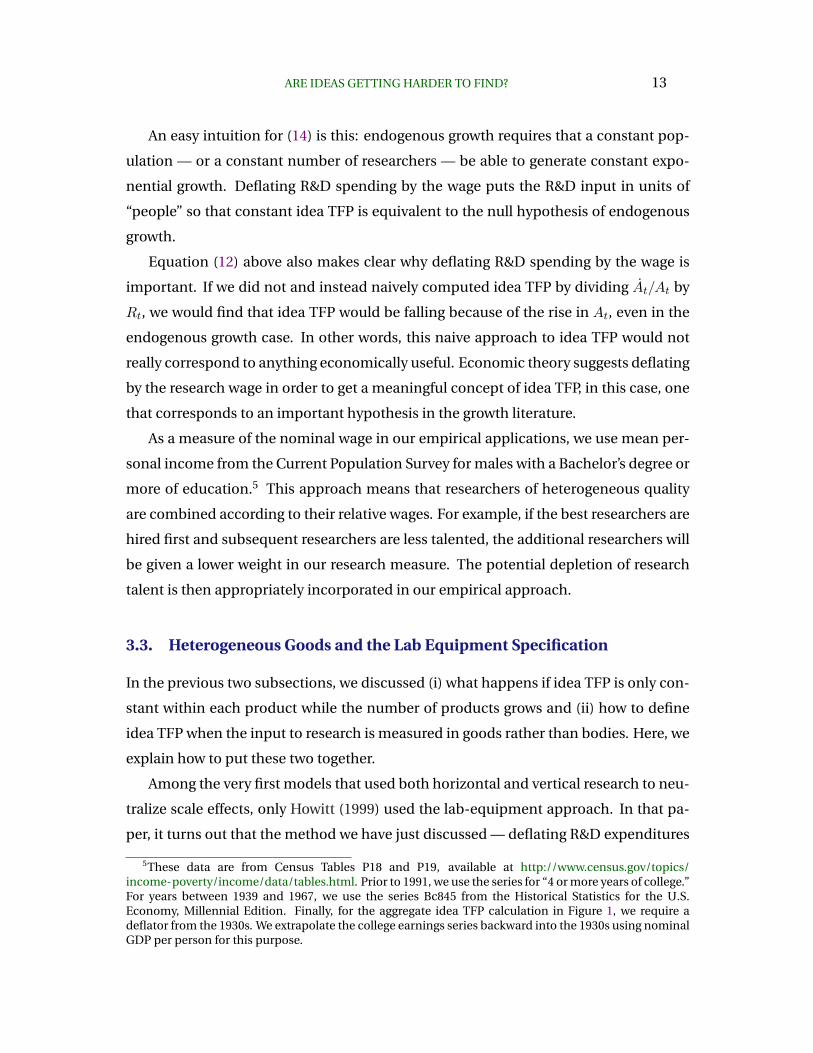
voted to improving crop yields. Figure 5 shows these measures for our four crops back
to the 1960s.13
12If such spillovers were larger at the start of our time period than at the end, we could be underestimat-ing the impact of semi-conductor R&D on productivity growth. We do not know of evidence suggestingthis.
13 For our measure of ideas, we use the national realized yields series for each crop available from theU.S. Department of Agriculture National Agricultural Statistics Service (2016). Our measure of R&D inputsconsists of the sum of R&D spending by the public and private sectors in the U.S. Data on private sectorbiological efficiency and crop protection R&D expenditures are from an updated USDA series based onFuglie et al. (2011), with the distribution of expenditure by crop taken from Perrin et al. (1983), Fernandez-Cornejo et al. (2004), Traxler et al. (2005), Huffman and Evenson (2006), and University of York (2016).Data on U.S. public sector R&D expenditure by crop are from the U.S. Department of Agriculture NationalInstitute of Food and Agriculture Current Research Information System (2016) and Huffman and Evenson(2006), with the distribution of expenditure by research focus taken from Huffman and Evenson (2006).
ARE IDEAS GETTING HARDER TO FIND? 21
Figure 5: U.S. Crop Yields
1960 1970 1980 1990 2000 2010 202040
60
80
100
120
140
160
180
BUSHELS/ACRE
(a) Corn
1960 1970 1980 1990 2000 2010 202020
25
30
35
40
45
50
BUSHELS/ACRE
(b) Soybeans
1960 1970 1980 1990 2000 2010 2020400
500
600
700
800
900
LBS/ACRE
(c) Cotton
1960 1970 1980 1990 2000 2010 202020
25
30
35
40
45
50
BUSHELS/ACRE
(d) Wheat
Note: Smoothed yields are computed using an HP filter with a smoothing parameter of 400.

22 BLOOM, JONES, VAN REENEN, AND WEBB
The figure show yields for each crop, measured in bushels or pounds harvested per
acre planted. These correspond to average yields realized on U.S. farms. They are there-
fore subject to many influences, including choice of inputs and random shocks. These
shocks, especially adverse weather and pest events, tend to have asymmetric effects:
adverse events cause much larger reductions in yields than favorable events increase
them, as indicated by the many large one-year reductions followed by recoveries in the
figure (see Huffman, Jin and Xu (2016)). Nevertheless, yields across these four crops
roughly doubled between 1960 and 2015.
Figure 6 shows the annualized average 5-year growth rate of yields (after smooth-
ing to remove shocks mostly due to weather). Yield growth has averaged around 1.5
percent per year since 1960 for these four crops, but with ample heterogeneity. These
5-year growth rates serve as our measure of idea output in studying the idea production
function for seed yields.
The green lines in Figure 6 show measures of the “effective” number of researchers
working on each crop, measured as the sum of public and private R&D spending de-
flated by the wage of high-skilled workers. Two measures are presented. The faster-
rising number corresponds to research targeted only at so-called biological efficiency.
This includes cross-breeding (hybridization) and genetic modification directed at in-
creasing yields, both directly and indirectly via improving insect resistance, herbicide
tolerance, and efficency of nutrient uptake, for example. The slower-growing number
additionally includes research on crop protection and maintenance, which includes
the development of herbicides and pesticides. The effective number of researchers
has grown sharply since 1969, rising by a factor that ranges from 3 to more than 25,
depending on the crop and the research measure.
It is immediately evident from comparing Figures 6 that idea TFP has fallen sharply
for agricultural yields: yield growth is relatively stable or even declining, while the
effective research that has driven this yield growth has risen tremendously. Idea TFP
is simply the ratio of average yield growth divided by the number of researchers.
Table 2 summarizes the idea TFP calculation for seed yields. As already noted,
the effective number of researchers working to improve seed yields rose enormously
between 1969 and 2009. For example, the increase was more than a factor of 23 for
both corn and soybeans if we restrict attention to seed-yield research narrowly-defined.
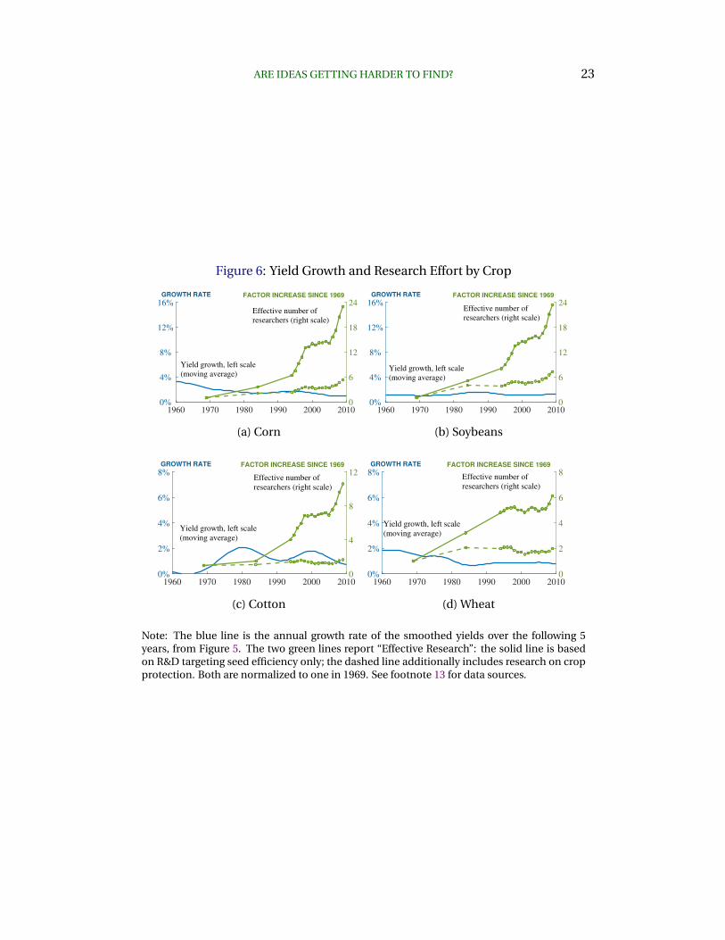
ARE IDEAS GETTING HARDER TO FIND? 23
Figure 6: Yield Growth and Research Effort by Crop
1960 1970 1980 1990 2000 20100%
4%
8%
12%
16%
Yield growth, left scale
(moving average)
Effective number of
researchers (right scale)
GROWTH RATE
0
6
12
18
24FACTOR INCREASE SINCE 1969
(a) Corn
1960 1970 1980 1990 2000 20100%
4%
8%
12%
16%
Yield growth, left scale
(moving average)
Effective number of
researchers (right scale)
GROWTH RATE
0
6
12
18
24FACTOR INCREASE SINCE 1969
(b) Soybeans
1960 1970 1980 1990 2000 20100%
2%
4%
6%
8%
Yield growth, left scale
(moving average)
Effective number of
researchers (right scale)
GROWTH RATE
0
4
8
12FACTOR INCREASE SINCE 1969
(c) Cotton
1960 1970 1980 1990 2000 20100%
2%
4%
6%
8%
Yield growth, left scale
(moving average)
Effective number of
researchers (right scale)
GROWTH RATE
0
2
4
6
8FACTOR INCREASE SINCE 1969
(d) Wheat
Note: The blue line is the annual growth rate of the smoothed yields over the following 5years, from Figure 5. The two green lines report “Effective Research”: the solid line is basedon R&D targeting seed efficiency only; the dashed line additionally includes research on cropprotection. Both are normalized to one in 1969. See footnote 13 for data sources.

24 BLOOM, JONES, VAN REENEN, AND WEBB
Table 2: Idea TFP Results by Crop, 1969–2009
— Effective research — — Idea TFP —Factor Average Factor Average
Crop increase growth decrease growth
Research on seed efficiency only
Corn 23.0 7.8% 52.2 -9.9%
Soybeans 23.4 7.9% 18.7 -7.3%
Cotton 10.6 5.9% 3.8 -3.4%
Wheat 6.1 4.5% 11.7 -6.1%
Research includes crop protection
Corn 5.3 4.2% 12.0 -6.2%
Soybeans 7.3 5.0% 5.8 -4.4%
Cotton 1.7 1.3% 0.6 +1.3%
Wheat 2.0 1.7% 3.8 -3.3%
Note: In the first panel of results, the research input is based on R&D expenditures for seedefficiency only. The second panel additionally includes research on crop protection. R&Dexpenditures are deflated by a measure of the nominal wage for high-skilled workers.
ARE IDEAS GETTING HARDER TO FIND? 25
If yield growth were constant (which is not a bad approximation across the four crops
as shown in Figure 6), then idea TFP would on average decline by this same factor. The
last 2 columns of Table 2 show this to be the case. On average, idea TFP declines for
crop yields by about 6 percent per year using the narrow definition of research and by
about 4 percent per year using the broader definition.
6. Mortality and Life Expectancy
Health expenditures account for around 18 percent of U.S. GDP, and a healthy life is
one of the most important goods we purchase. Our third collection of industry case
studies examines the productivity of medical research.
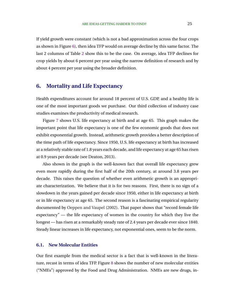
Figure 7 shows U.S. life expectancy at birth and at age 65. This graph makes the
important point that life expectancy is one of the few economic goods that does not
exhibit exponential growth. Instead, arithmetic growth provides a better description of
the time path of life expectancy. Since 1950, U.S. life expectancy at birth has increased
at a relatively stable rate of 1.8 years each decade, and life expectancy at age 65 has risen
at 0.9 years per decade (see Deaton, 2013).
Also shown in the graph is the well-known fact that overall life expectancy grew
even more rapidly during the first half of the 20th century, at around 3.8 years per
decade. This raises the question of whether even arithmetic growth is an appropri-
ate characterization. We believe that it is for two reasons. First, there is no sign of a
slowdown in the years gained per decade since 1950, either in life expectancy at birth
or in life expectancy at age 65. The second reason is a fascinating empirical regularity
documented by Oeppen and Vaupel (2002). That paper shows that “record female life
expectancy” — the life expectancy of women in the country for which they live the
longest — has risen at a remarkably steady rate of 2.4 years per decade ever since 1840.
Steady linear increases in life expectancy, not exponential ones, seem to be the norm.
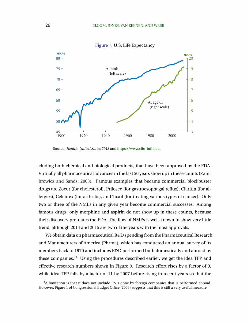
6.1. New Molecular Entities
Our first example from the medical sector is a fact that is well-known in the litera-
ture, recast in terms of idea TFP. Figure 8 shows the number of new molecular entities
(“NMEs”) approved by the Food and Drug Administration. NMEs are new drugs, in-
26 BLOOM, JONES, VAN REENEN, AND WEBB
Figure 7: U.S. Life Expectancy
1900 1920 1940 1960 1980 200045
50
55
60
65
70
75
80
At birth
(left scale)
At age 65
(right scale)
YEARS
13
14
15
16
17
18
19
20YEARS
Source: Health, United States 2013 and https://www.clio-infra.eu.
cluding both chemical and biological products, that have been approved by the FDA.
Virtually all pharmaceutical advances in the last 50 years show up in these counts (Zam-
browicz and Sands, 2003). Famous examples that became commercial blockbuster
drugs are Zocor (for cholesterol), Prilosec (for gastroesophagal reflux), Claritin (for al-
lergies), Celebrex (for arthritis), and Taxol (for treating various types of cancer). Only
two or three of the NMEs in any given year become commercial successes. Among
famous drugs, only morphine and aspirin do not show up in these counts, because
their discovery pre-dates the FDA. The flow of NMEs is well-known to show very little
trend, although 2014 and 2015 are two of the years with the most approvals.
We obtain data on pharmaceutical R&D spending from the Pharmaceutical Research
and Manufacturers of America (Phrma), which has conducted an annual survey of its
members back to 1970 and includes R&D performed both domestically and abroad by
these companies.14 Using the procedures described earlier, we get the idea TFP and
effective research numbers shown in Figure 9. Research effort rises by a factor of 9,
while idea TFP falls by a factor of 11 by 2007 before rising in recent years so that the
14A limitation is that it does not include R&D done by foreign companies that is performed abroad.However, Figure 1 of Congressional Budget Office (2006) suggests that this is still a very useful measure.
ARE IDEAS GETTING HARDER TO FIND? 27
Figure 8: New Molecular Entities Approved by the FDA
1970 1975 1980 1985 1990 1995 2000 2005 2010 2015
0
10
20
30
40
50
60
YEAR
NUMBER OF NMES APPROVED
Note: Historical data on NME approvals are from Food and Administration(2013). Data for recent years are taken from Pharmaceutical Research andManufacturers of America (2016).
overall decline by 2014 is a factor of 5. Over the entire period, research effort rises at an
annual rate of 6.0 percent, while idea TFP falls at an annual rate of 3.5 percent.
Of course, it is far from obvious that simple counts of NMEs appropriately measure
the output of ideas; we’d really like to know how important each innovation is. In
addition, the NMEs still suffer from an important aggregation issue, adding up across
a wide range of health conditions. These limitations motivate the approach described
next.15
6.2. Mortality
Consider a person who faces an two age-invariant Poisson processes for dying, with
arrival rates δ1 and δ2. We think of δ1 as reflecting a particular disease we are studying,
such as cancer or heart disease, and δ2 as capturing all other sources of mortality. The
probability a person lives for at least x years before succumbing to type i mortality is
15Lichtenberg (2016) provides a complementary approach in using NMEs to measure the output of ideasand their value. He studies NME approvals by cancer site and shows that each new approval is associatedwith a reduction in years of life lost before age 75 of 2.3%.

28 BLOOM, JONES, VAN REENEN, AND WEBB
Figure 9: Idea TFP for New Molecular Entities
1970 1975 1980 1985 1990 1995 2000 2005 2010 20151/16
1/8
1/4
1/2
1
Idea TFP (left scale)
Effective number of
researchers (right scale)
INDEX (1970=1)
1
2
4
8
16INDEX (1970=1)
Note: Historical data on NME approvals are from Food and Administration(2013). Data on research spending by the pharmaceutical industry are from the2010, 2013, and 2016 editions of Pharmaceutical Research and Manufacturers ofAmerica (2016).
the survival rate Si(x) = e−δix, and the probability the person lives for at least x years
before dying from any cause is S(x) = S1(x)S2(x) = e−(δ1+δ2)x. Life expectancy at age
a, LE(a) is then well known to equal
LE(a) =
∫ ∞0
S(x)dx =
∫ ∞0
e−(δ1+δ2)xdx =1
δ1 + δ2. (15)
Now consider how life expectancy changes if the type imortality rate changes slightly.
It is easy to show that the expected years of life saved by the mortality change is
dLE(a) =δi
δ1 + δ2· LE(a) ·
(−dδiδi
). (16)
That is, the expected years of life saved from a decline in, say, cancer mortality is the
product of three terms. First is the share of cancer mortality in overall mortality. Second
is the overall level of life expectancy at age a itself, and finally is the percentage decline
in cancer mortality.16
16The assumption of constant mortality by age is a simplification. A better approximation is Gompertz

ARE IDEAS GETTING HARDER TO FIND? 29
As discussed at the start of this section, life expectancy tends to rise linearly. There-
fore, constant exponential growth in income per person is associated with constant
arithmetic increases in life expectancy, which in the aggregate average 1.8 years per
decade in the U.S. We therefore take the quantity described in equation (16) as our
measure of the output of ideas associated with declines in mortality for a given dis-
ease.17
The research input aimed at reducing mortality from a given disease is at first blush
harder to measure. For example, it is difficult to get research spending broken down
into spending on various diseases. Nevertheless, we think we have a useful solution
to this problem: we measure the number of scientific publications in PUBMED that
have “cancer,” for example, as a MESH (Medical Subject Heading) term. MESH is the
National Library of Medicine’s controlled vocabulary thesaurus.18 We do this in two
ways. Our broader approach (“publications”) uses all publications with the appropriate
MESH keyword as our input measure. Our narrower approach (“trials”) further restricts
our measure to those publications that according to MESH correspond to a clinical
trial. Rather than using scientific publications as an output measure, as other studies
have done, we use publications and clinical trials as input measures to capture research
effort aimed at reducing mortality for a particular disease.
Figure 10 shows our basic “idea output” measures for mortality from all cancers and
from breast cancer. The 5-year mortality rate conditional on being diagnosed with ei-
ther type of cancer shows an S-shaped decline since 1975. This translates into a hump-
shaped “Years of life saved per 1000 people” — the empirical analog of equation (16) —
as the mortality rate first rises and then slows. For example, for all cancers, the years of
life saved series peaks around 1990 at more than 100 years of life saved per 1000 people
before declining to around 60 years in the 2000s.
Figure 11 shows our research input measure based on PUBMED publication statis-
Law, which says that mortality rises exponentially with age. The formulas with this approximation do notwork out well, however, so we have not yet pursued this approach.
17Our measures of life expectancy and mortality from all sources by age come from the Human MortalityDatabase at http://mortality.org. To measure the percentage declines in mortality rates from cancer, weuse the age-adjusted mortality rates for U.S. women ages 50 and over computed from 5-year survival rates,taken from the National Cancer Institute’s Surveillance, Epidemiology, and End Results program at http://seer.cancer.gov/.
18For more information on MESH, see https://www.nlm.nih.gov/mesh/. Our queries of the PUBMEDdata use the webtool created by the Institute for Biostatistics and Medical Informatics (IBMI) MedicalFaculty, University of Ljubljana, Slovenia available at http://webtools.mf.uni-lj.si/.

30 BLOOM, JONES, VAN REENEN, AND WEBB
Figure 10: Mortality and Years of Life Saved
1975 1980 1985 1990 1995 2000 2005 20100.3
0.4
0.5
0.6
0.7
0.8
Years of life saved
per 1000 people (right scale)
5-year mortality rate
(left scale)
5-YEAR DEATH RATE
20
40
60
80
100
120YEARS
(a) All cancers
1975 1980 1985 1990 1995 2000 2005 20100.05
0.1
0.15
0.2
0.25
0.3
0.35
Years of life saved
per 1000 people (right scale)
5-year mortality rate
(left scale)
5-YEAR DEATH RATE
0
5
10
15
20
25
30YEARS
(b) Breast cancer
Note: The “5-year mortality rate” is computed as negative the log of the(smoothed) five-year survival rate for cancer for people ages 50 and higher,from the National Cancer Institute’s Surveillance, Epidemiology, and End Resultsprogram at http://seer.cancer.gov/. The “Years of life saved per 1000 people” iscomputed using equation (16), as described in the text.

ARE IDEAS GETTING HARDER TO FIND? 31
Table 3: Idea TFP Results for Medical Research, 1975–2006
— Effective research — — Idea TFP —Factor Average Factor Average
Disease increase growth decrease growth
All publications
Cancer, all types 3.5 4.0% 1.2 -0.6%
Breast cancer 5.4 5.4% 6.6 -6.1%
Clinical trials only
Cancer, all types 17.1 9.2% 5.9 -5.7%
Breast cancer 18.8 9.5% 22.8 -10.1%
Note: In the first panel of results, the research input is based on all publications inPUBMED with “cancer” or “breast cancer” as a MESH keyword. The second paneladditionally restricts the sample to only publications involving clinical trials.
tics. Total publications for all cancers increased by a factor of 3.5 between 1975 and
2006 (the years for which we’ll be able to compute idea TFP), while publications re-
stricted to clinical trials increased by a factor of 17.1 during this same period. A similar
pattern is seen for breast cancer research.
Idea TFP for our medical research applications is computed as the ratio of years
of life saved to the number of publications. Figure 12 shows our idea TFP measures.
The hump-shape present in the years-of-life-saved measure carries over here. Idea TFP
rises until the mid 1980s and then falls. Overall, between 1975 and 2006, idea TFP for all
cancers declines by a factor of 1.2 using all publications and a factor of 5.9 using clinical
trials. The declines for breast cancer are even larger, as shown in Table 3.
Several general comments about idea TFP for medical research deserve mention.
First, for this application, the units of idea TFP are different than what we’ve seen so
far. For example, between 1985 and 2006, declining idea TFP means that the number
of years of life saved per 100,000 people in the population by each publication of a
clinical trial declined from more than 8 years to just over one year. For breast cancer,
the changes are even starker: from around 16 years per clinical trial in the mid 1980s to
less than one year by 2006.

32 BLOOM, JONES, VAN REENEN, AND WEBB
Figure 11: Medical Research Effort
1960 1970 1980 1990 2000 2010 202025
100
400
1600
6400
25600
102400 Number of publications
Number for clinical trials
YEAR
RESEARCH ON CANCER
(a) All cancers
1960 1970 1980 1990 2000 2010 202025
50
100
200
400
800
1600
3200
6400
12800Number of publications
Number for clinical trials
YEAR
RESEARCH ON CANCER
(b) Breast cancer
Note: The number of publications and clinical trials related to cancer are takenfrom the PUBMED publications database, as described in the text.

ARE IDEAS GETTING HARDER TO FIND? 33
Figure 12: Idea TFP for Medical Research
Per clinical trial
Per 100 publications
1975 1980 1985 1990 1995 2000 2005 2010YEAR
1
2
4
8
16
32
YEARS OF LIFE SAVED PER 100,000 PEOPLE
(a) All cancers
Per clinical trial
Per 100 publications
1975 1980 1985 1990 1995 2000 2005 2010YEAR
1/2
1
2
4
8
16
32
64
128
YEARS OF LIFE SAVED PER 100,000 PEOPLE
(b) Breast cancer
Note: Idea TFP is computed as the ratio of years of life saved to the number ofpublications.
34 BLOOM, JONES, VAN REENEN, AND WEBB
Next, however, notice that the changes were not monotonic if we go back to 1975.
Between 1975 and the mid-1980s, idea TFP for these two medical research categories
increased quite substantially. The production function for new ideas is obviously com-
plicated and heterogeneous. These cases suggest that it may get easier to find new ideas
at first before getting harder, at least in some areas.
7. Idea TFP in Firm-Level Data
The case studies considered so far are useful for many reasons already explained. How-
ever, at the end of the day, they are just case studies, and one naturally wonders how
representative they are of the broader economy. In addition, some growth models
associate each firm with a different variety: perhaps the number of firms making corn
or semiconductor chips is rising sharply, so that research effort per firm is actually
constant, as is idea TFP at the firm level. Declining idea TFP for corn or semiconductors
could in this view simply reflect a further composition bias.19
To help address these concerns, we turn to Compustat data on US publicly-traded
firms. The strength of these data is that they are more representative than the case
studies, but of course they too have limitations. Publicly-traded firms are still a select
sample, and our measures of “ideas” and research inputs are likely less precise. How-
ever, as a complement to the case studies, we find this evidence helpful.
As a measure of the output of the idea production function, we use decadal averages
of annual growth in sales revenue, market capitalization, and employment within each
firm. We take the decade as our period of observation to smooth out fluctuations.
Why would growth in sales revenue, market cap, or employment be informative
about a firm’s production of ideas? This approach follows a recent literature empha-
sizing precisely these links. Many papers have shown that news of patent grants for a
firm has a large immediate effect on the firm’s stock market capitalization (e.g. Blun-
dell, Griffith and Van Reenen, 1999; Kogan, Papanikolaou, Seru and Stoffman (2015)).
Patents are also positively correlated with the firm’s subsequent growth in employment
and sales.
19For example, Peretto (1998) and Peretto (2016b) emphasize this perspective on varieties, while Aghionand Howitt (1992) take the alternative view that different firms may be involved in producing the samevariety. Klette and Kortum (2004) allow the number of varieties produced by each firm to be heterogeneousand to evolve over time.

ARE IDEAS GETTING HARDER TO FIND? 35
More generally, in models in the tradition of Lucas (1978), Hopenhayn (1992), and
Melitz (2003), increases in the fundamental productivity of a firm show up in the long
run as increases in sales and firm size, but not as increases in sales revenue per worker.20 This motivates our use of sales revenue or employment to measure fundamental
productivity. Hsieh and Klenow (2009) and Garcia-Macia, Hsieh and Klenow (2016) are
recent examples of papers that follow a related approach. Of course, in more general
models with fixed overhead labor costs, sales revenue per worker and TFPR can be re-
lated to fundamental productivity (e.g. Bartelsman, Haltiwanger and Scarpetta, 2013).
And sales revenue and employment can change for reasons other than the discovery of
new ideas. We try to address these issues by also looking at revenue productivity and
various sample selection procedure, discussed below. These problems also motivate
the earlier approach of looking at case studies.
To measure the research input, we use a firm’s spending on research and devel-
opment from Compustat. This means we are restricted to firms that report formal
R&D, and such firms are well-known to be a select sample (e.g. disproportionately in
manufacturing and large). We look at firms since 1980 that report non-zero R&D, and
this restricts us to an initial sample of 15,128 firms. Our additional requirements for
sample selection in our baseline sample are
1. We observe at least 3 annual growth observations for the firm in a given decade.
These growth rates are averaged to form the idea output growth measure for that
firm in that decade.
2. We only consider decades in which our idea output growth measure for the firm
is positive (negative growth is clearly not the result of the firm innovating, and our
framework cannot make sense of negative idea TFP).
3. We require the firm to be observed (for both the output growth measure and the
research input measure) for two consecutive decades. Our decades are the 1980s,
20This is obvious when one thinks about the equilibrium condition for the allocation of labor acrossfirms in simple settings: in equilibrium, a worker must be indifferent between working in two differentfirms, which equalizes wages. But wages are typically proportional to output per worker. Moreover, withCobb-Douglas production and a common exponent on labor, sales revenue per worker would be preciselyequated across firms even if they had different underlying productivities. In a Lucas (1978) span of controlsetting, more productive firms just hire more workers, which drives down the marginal product until it isequated across firms. In alternative settings with monopolistic competition, it is the price of a particularvariety that declines as the firm expands. Regardless, higher fundamental productivity shows up as higheremployment or sales revenue, but not in higher sales per employee.
36 BLOOM, JONES, VAN REENEN, AND WEBB
the 1990s, the 2000s (which refers to the 2000-2007 period), and the 2010s (which
refers to the 2010-2015 period); we drop the years 2008 and 2009 because of the
financial crisis.
We relax many of these conditions in our robustness checks.
Table 4 shows our idea TFP calculation for various cuts of the Compustat data:
using sales revenue, market cap, and employment as our idea output measure and
following firms that we observe for two, three, and four decades. In all samples, there
is substantial growth in the average number of effective number of researchers within
each firm, with growth rates averaging between 5.6% and 8.8% per year. Under our null
hypothesis, this rapid growth in research should translate into higher growth rates of
firm-level sales and employment with a constant level of idea TFP. Instead, what we see
in Table 4 are steady, rapid declines in firm-level idea TFP across all samples, at growth
rates that range from -8.8% to -14.5% per year for multiple decades.
Put differently, and reporting the results using sales revenue as a baseline, idea TFP
declines by an average factor of 3.9 for firms that we can compare across only two
decades, by a factor of 9.2 across firms we can compare across three decades, and by
a factor of 40.3 across firms that we can compare across our entire 4 decade sample,
between 1980 and 2015.21
Averaging across all our samples, idea TFP falls at a rate of about 11% per year,
cumulating to a 3-fold decline every decade. At this rate, idea TFP declines by a factor
of more than 25 over three decades of changes; put differently, it requires 25 times more
researchers today than it did 30 years ago to produce the same rate of economic growth.
The next three figures characterize the heterogeneity across firms in our Compustat
sample by showing the distribution of the factor changes in effective research and idea
TFP across all the firms; to keep things manageable, we focus on the results for sales
revenue, but the results with other output measures are similar. Figure 13 shows this
distribution for the firms we observe for only two decades, while Figures 14 and 15
shows the distributions for the firms observed for three and four decades.
The heterogeneity across firms is impressive and somewhat reminiscent of the het-
erogeneity we see in our case studies. Nevertheless, it is clear from these histograms
that there is essentially no evidence that constant idea TFP is a good characterization
21The averages we report throughout are weighted averages, using the effective number of researchersin each firm as weights.

ARE IDEAS GETTING HARDER TO FIND? 37
Table 4: Idea TFP Results using Compustat Firm-Level Data
— Effective research — — Idea TFP —Factor Average Factor Average
Sample increase growth decrease growth
Sales Revenue
2 decades (1712 firms) 2.0 6.8% 3.9 -13.6%
3 decades (469 firms) 3.8 6.7% 9.2 -11.1%
4 decades (149 firms) 13.7 8.7% 40.3 -12.3%
Market Cap
2 decades (1124 firms) 2.2 8.0% 3.4 -12.2%
3 decades (335 firms) 3.1 5.6% 6.3 - 9.2%
4 decades (125 firms) 7.9 6.9% 14.0 -8.8%
Employment
2 decades (1395 firms) 2.2 8.0% 2.8 -10.3%
3 decades (319 firms) 4.0 6.9% 18.2 -14.5%
4 decades (101 firms) 13.9 8.8% 31.5 -11.5%
Note: The table shows averages of firm-level outcomes for effective research and ideaTFP. Sales Revenue and Market Cap are deflated by the GDP implicit price deflator. R&Dexpenditures are deflated by a measure of the nominal wage. The average growth rateacross 2 decades is computed by dividing by 10 years (e.g. between 1985 and 1995); othersfollow this same approach. Averages are computed by weighting firms by the mediannumber of effective researchers in each firm across the decades.

38 BLOOM, JONES, VAN REENEN, AND WEBB
Figure 13: Compustat Distributions, Sales Revenue (2 Decades)
Note: Based on 1712 firms. 22.1% of firms have increasing idea TFP. Only 3.0%have idea TFP that is roughly constant, defined as a growth rate whose absolutevalue is less than 1% per year.
Figure 14: Compustat Distributions, Sales Revenue (3 Decades)
Note: Based on 469 firms. 11.9% of firms have increasing idea TFP. Only 4.3%have idea TFP that is roughly constant, defined as a growth rate whose absolutevalue is less than 1% per year.

ARE IDEAS GETTING HARDER TO FIND? 39
Figure 15: Compustat Distributions, Sales Revenue (4 Decades)
Note: Based on 149 firms. 14.8% of firms have increasing idea TFP. 4.7% firmsin this sample have idea TFP that is roughly constant, defined as a growth ratewhose absolute value is less than 1% per year.
of the firm-level data. The average, median, and modal firms experience large declines
in idea TFP. There is a long tail of firms experiencing even larger declines but also a
small minority of firms that see increases in idea TFP. The fraction of firms that exhibit
something like constant idea TFP is tiny. For example, less than 5% of firms in any of
the histograms have idea TFP changing (either rising or falling) by less than 1% per year
on average.
Table 5 provides additional evidence of the robustness of these results. In the inter-
ests of brevity, we report these results for the sales revenue output measure for firms
that we observe across three decades, but the results for our other output measures
and time frames are similar. The first row of the table repeats the benchmark results
described earlier. The second row imposes the restriction that research is increasing
across the observed decades. The third row tightens our restrictions and drops firm
in which sales revenue declines on average in any decade.The fourth row uses median
sales growth in each decade rather than mean sales growth as our output measure.
And the fifth row reports unweighted averages rather than weighting the firms by the
effective number of researchers. The general finding of substantial declines in idea TFP
is robust.

40 BLOOM, JONES, VAN REENEN, AND WEBB
Table 5: Compustat Sales Data across 3 Decades: Robustness
— Effective research — — Idea TFP —Factor Average Factor Average
Case increase growth decrease growth
Benchmark (469 firms) 3.8 6.7% 9.2 -11.1%
Research must increase (356 firms) 5.1 8.1% 11.6 -12.3%
Drop if any negative growth (367 firms) 5.6 8.6% 17.9 -14.4%
Median sales growth (586 firms) 3.8 6.6% 6.3 -9.2%
Unweighted averages (469 firms) 3.8 6.7% 9.2 -11.1%
Note: Robustness results reported for the sample of changes across 3 decades. “Research must increase”means we require that the research measure be rising across the decades. “Drop if any negative growth”means we drop firms that have any decade (across our 1980–2015 period) in which average market capgrowth is negative. “Median sales growth” uses the median of sales revenue growth in each decade ratherthan the mean. “Unweighted averages” gives each firm equal weight in computing summary statistics,rather than weighting each firm by its effective number of researchers.
8. Discussion
The evidence presented in this paper concerns the extent to which a constant level
of research effort can generate constant exponential growth, either in the economy
as a whole or within relatively narrow categories, such as a firm or a seed type or a
health condition. We provide consistent evidence that the historical answer to this
question is no: as summarized in Table 6, idea TFP is declining at a substantial rate in
virtually every place we look. The table also provides a way to quantify the magnitude
of the declines in idea TFP by reporting the half-life in each case. Taking the aggregate
economy number as a representative example, idea TFP declines at an average rate of
5.3 percent per year, meaning that it takes around 13 years for idea TFP to fall by half.
Or put another way, the economy has to double its research efforts every 13 years just
to maintain the same overall rate of economic growth.
A natural question is whether or not these empirical patterns can be reproduced in
a general equilibrium model of growth. One class of models that is broadly consistent
with this evidence is the semi-endogenous growth approach of Jones (1995), Kortum

ARE IDEAS GETTING HARDER TO FIND? 41
Table 6: Summary of the Evidence on Idea TFP
Average annual Half-life Extent ofTime growth rate of idea TFP Diminishing
Scope Period of idea TFP (years) Returns, β
Aggregate economy 1930–2015 -5.3% 13 3.4
Moore’s law (narrow) 1971–2014 -7.5% 9 0.22
Moore’s law (baseline) 1971–2014 -10.1% 7 0.29
Corn, version 1 1969–2009 -9.9% 7 7.2
Corn, version 2 1969–2009 -6.2% 11 4.5
Soybeans, version 1 1969–2009 -7.3% 9 6.3
Soybeans, version 2 1969–2009 -4.4% 16 3.8
Cotton, version 1 1969–2009 -3.4% 21 2.5
Cotton, version 2 1969–2009 +1.3% -55 -0.9
Wheat, version 1 1969–2009 -6.1% 11 6.8
Wheat, version 2 1969–2009 -3.3% 21 3.7
New molecular entities 1970–2015 -3.5% 20 ...
Cancer (all), publications 1975–2006 -0.6% 116 ...
Cancer (all), trials 1975–2006 -5.7% 12 ...
Breast cancer, publications 1975–2006 -6.1% 11 ...
Breast cancer, trials 1975–2006 -10.1% 7 ...
Heart disease, publications ...
Heart disease, trials ...
Compustat, sales 3 decades -11.1% 6 1.1
Compustat, market cap 3 decades -9.2% 8 0.9
Compustat, employment 3 decades -14.5% 5 1.8
Note: The growth rates of idea TFP are taken from other tables in this paper. The half life is the numberof years it takes for idea TFP to fall in half at this growth rate. The last column reports the extent ofdiminishing returns in producing exponential growth, according to equation (17). This measure is onlyreported for cases in which the idea output measure is anexponential growth rate (i.e. not for the healthtechnologies).

42 BLOOM, JONES, VAN REENEN, AND WEBB
(1997), and Segerstrom (1998).22 These models propose that the idea production func-
tion takes the formAtAt
= αSt
Aβt=⇒ iTFPt =
α
Aβt. (17)
Idea TFP declines as At rises, so that it gets harder and harder to generate constant
exponential growth. The elasticity β governs this process. That is, it measures the extent
of dynamic diminishing returns in idea production, with a higher β meaning that idea
TFP declines more rapidly as At increases.
Comparing both sides of the first equation in (17), one can see that constant expo-
nential growth requires a growing number of researchers St. In fact, if At/At is constant
over time, it must be that the numerator and denominator of the right-hand side of that
equation grow at the same rate. This means that constant exponential growth requires
gA =gSβ
(18)
where gx denotes the constant growth rate of any variable x. The growth rate of the
economy equals the growth rate of research effort deflated by the extent of diminishing
returns in idea production. Rising research effort and declining idea TFP offset —
endogenously in this framework — to deliver constant exponential growth.
Finally, this analysis can be applied across different firms, goods, or industries, fol-
lowing the insights of Ngai and Samaniego (2011), who develop a semi-endogenous
growth model with heterogeneity in the dynamic spillover parameters of the idea pro-
duction functions. Some goods, like semiconductors, can have rapid productivity growth
because their β is small, while other goods like the speed of airplanes or perhaps the
education industry itself could have slow rates of innovation because their β is large.
Nevertheless, all of these products could exhibit constant exponential growth if the
amount of research effort put toward innovation is itself growing exponentially.
This framework helps us to address a phenomenon that might at first have appeared
puzzling: idea TFP is declining most rapidly in the fastest growing sector in the econ-
omy, semiconductors. Why? In particular, why are we throwing so many resources at a
sector that has the sharpest declines in idea TFP?
The last column of Table 6 reports estimates of β for each of our case studies, ac-
22Jones (2005) provides a broad overview of this class of models.

ARE IDEAS GETTING HARDER TO FIND? 43
cording to equation (17), and the results speak to the semiconductor puzzle we just
highlighted. In particular, semiconductors is the application with the smallest value of
β, coming in at 0.29, suggesting that it is the sector with the least degree of diminishing
returns in idea production: A is growing at 35% per year, while idea TFP is falling at 10%
per year. From (17), this implies a value of β of 10/35 ≈ 0.3 In contrast, economy-wide
TFP growth averages about 1.5% per year, while idea TFP is declining at a rate of about
5% per year, yielding a β of more than 3! So in fact, semiconductors shows much less
diminishing returns than the economy as a whole.
Idea TFP for semiconductors falls so rapidly, not because that sector has the sharpest
diminishing returns — the opposite is true. It is instead because research in that sector
is growing more rapidly than in any other part of the economy, pushing idea TFP down.
A plausible explanation for the rapid research growth in this sector is the “general pur-
pose” nature of information technology. Demand for better computer chips is growing
so fast that it is worth suffering the declines in idea TFP there in order to achieve the
gains associated with Moore’s Law.
One way in which the overall interpretation of the evidence in this paper could be
wrong is if there is indeed declining idea TFP in every sector, but the entire increase
in aggregate R&D occurs in making quality/productivity improvements for individual
varieties. The separate idea production function for producing new varieties could then
exhibit constant idea TFP if in fact the research going to create new varieties is not
increasing over time. While this is conceptually possible, it seems unlikely. We do not
have any growth models in the literature that suggest this could occur in an equilibrium
in which there is population growth. Why, despite a growing population and constant
idea TFP, would the equilibrium allocation feature a constant number of researchers
creating new varieties? Nevertheless, this loophole is one that future research may wish
to consider.
9. Conclusion
A key assumption of many endogenous growth models is that a constant number of
researchers can generate constant exponential growth. We show that this assumption
corresponds to the hypothesis that the total factor productivity of the idea production

44 BLOOM, JONES, VAN REENEN, AND WEBB
function is constant, and we proceed to measure idea TFP in many different contexts.
Our robust finding is that idea TFP is falling sharply everywhere we look. Taking the
U.S. aggregate number as representative, idea TFP falls in half every 13 years — ideas
are getting harder and harder to find. Put differently, just to sustain constant growth in
GDP per person, the U.S. must double the amount of research effort searching for new
ideas every 13 years to offset the increased difficulty of finding new ideas.
This analysis also has implications for the growth models that economists use in
our own research, like those cited in the introduction. The standard approach in recent
years is to use models that assume constant idea TFP, in part because it is convenient
and in part because the earlier literature has been interpreted as being inconclusive on
the extent to which this is problematic. We believe the empirical work we’ve presented
speaks clearly against this assumption. A first order fact of growth empirics is that idea
TFP is falling sharply.
That this particular aspect of endogenous growth theory should be reconsidered
does not diminish the contribution of that literature. Quite the contrary. The only
reason models with declining idea TFP can sustain exponential growth in living stan-
dards is because of the key insight from that literature: ideas are nonrival. And if idea
TFP were constant, sustained growth would actually not require that ideas be nonrival;
Akcigit, Celik and Greenwood (2016) show that fully rivalrous ideas in a model with
perfect competition can generate sustained exponential growth in this case. Our pa-
per therefore clarifies that the fundamental contribution of endogenous growth theory
is not that idea TFP is constant or that subsidies to research can permanently raise
growth. Rather it is that ideas are different from all other goods in that they do not get
depleted when used by more and more people. Exponential growth in research leads to
exponential growth in At. And because of nonrivalry, this leads to exponential growth
in per capita income.
References
Acemoglu, Daron and Pascual Restrepo, “The Race between Man and Machine: Implications of
Technology for Growth, Factor Shares and Employment,” May 2016. unpublished.

ARE IDEAS GETTING HARDER TO FIND? 45
Aghion, Philippe and Peter Howitt, “A Model of Growth through Creative Destruction,” Econo-
metrica, March 1992, 60 (2), 323–351.
and , Endogenous Growth Theory, Cambridge, MA: MIT Press, 1998.
, Ufuk Akcigit, and Peter Howitt, “What Do We Learn From Schumpeterian Growth Theory?,”
in “Handbook of Economic Growth,” Vol. 2 of Handbook of Economic Growth, Elsevier, 2014,
chapter 1, pp. 515–563.
Akcigit, Ufuk, Murat Alp Celik, and Jeremy Greenwood, “Buy, Keep, or Sell: Economic Growth
and the Market for Ideas,” Econometrica, 2016, 84 (3), 943–984.
Congressional Budget Office, “Research and Development in the Pharmaceutical Industry,”
Technical Report October 2006.
Cowen, Tyler, The Great Stagnation: How America Ate All The Low-Hanging Fruit of Modern
History, Got Sick, and Will (Eventually) Feel Better: A Penguin eSpecial from Dutton, Penguin
Group US, 2011.
Dinopoulos, Elias and Constantinos Syropoulos, “Rent Protection as a Barrier to Innovation and
Growth,” Economic Theory, 2007, 32 (2), 309–332.
and Peter Thompson, “Schumpeterian Growth without Scale Effects,” Journal of Economic
Growth, December 1998, 3 (4), 313–335.
Fernandez-Cornejo, Jorge et al., “The seed industry in US agriculture: An exploration of
data and information on crop seed markets, regulation, industry structure, and research
and development,” Technical Report, United States Department of Agriculture, Economic
Research Service 2004.
Flamm, Kenneth, “Has Moore’s Law Been Repealed? An Economist’s Perspective,” Computers
in Science and Engineering, forthcoming.
Food and Drug Administration, “Summary of NDA Approvals & Receipts, 1938 to the present,”
2013. Online data report.
Fuglie, Keith, Paul Heisey, John L King, Kelly Day-Rubenstein, David Schimmelpfennig,
Sun Ling Wang, Carl E Pray, and Rupa Karmarkar-Deshmukh, “Research investments and
market structure in the food processing, agricultural input, and biofuel industries world-
wide,” USDA-ERS Economic Research Report, 2011, (130).
Garcia-Macia, Daniel, Chang-Tai Hsieh, and Peter J. Klenow, “How Destructive is Innovation?,”
April 2016. Unpublished manuscript.

46 BLOOM, JONES, VAN REENEN, AND WEBB
Gordon, Robert J., The Rise and Fall of American Growth: The US Standard of Living since the
Civil War, Princeton University Press, 2016.
Griliches, Zvi, “Productivity, R&D and the Data Constraint,” American Economic Review, March
1994, 84 (1), 1–23.
Grossman, Gene M. and Elhanan Helpman, Innovation and Growth in the Global Economy,
Cambridge, MA: MIT Press, 1991.
Ha, Joonkyung and Peter Howitt, “Accounting for trends in productivity and R&D: A Schum-
peterian critique of semi-endogenous growth theory,” Journal of Money, Credit and Banking,
2007, 39 (4), 733–774.
Hopenhayn, Hugo A., “Entry, Exit, and Firm Dynamics in Long-Run Equilibrium,” Economet-
rica: Journal of the Econometric Society, 1992, pp. 1127–1150.
Howitt, Peter, “Steady Endogenous Growth with Population and R&D Inputs Growing,” Journal
of Political Economy, August 1999, 107 (4), 715–730.
Hsieh, Chang-Tai and Peter J. Klenow, “Misallocation and Manufacturing TFP in China and
India,” Quarterly Journal of Economics, 2009, 124 (4), 1403–1448.
Huffman, Wallace E and Robert E Evenson, Science for agriculture: A long-term perspective, John
Wiley & Sons, 2006.
Huffman, Wallace E., Yu Jin, and Zheng Xu, “The economic impacts of technology and climate
change: new evidence from U.S. corn yields,” May 2016. Working Paper.
Jones, Benjamin F., “The Burden of Knowledge and the Death of the Renaissance Man: Is
Innovation Getting Harder?,” Review of Economic Studies, 2009, 76 (1).
Jones, Charles I., “R&D-Based Models of Economic Growth,” Journal of Political Economy,
August 1995, 103 (4), 759–784.
, “Growth and Ideas,” in Philippe Aghion and Steven A. Durlauf, eds., Handbook of Economic
Growth, New York: North Holland, 2005, pp. 1063–1111.
and Jihee Kim, “A Schumpeterian Model of Top Income Inequality,” October 2014. Stanford
University manuscript.
Klette, Tor Jakob and Samuel Kortum, “Innovating Firms and Aggregate Innovation,” Journal of
Political Economy, October 2004, 112 (5), 986–1018.

ARE IDEAS GETTING HARDER TO FIND? 47
Kogan, Leonid, Dimitris Papanikolaou, Amit Seru, and Noah Stoffman, “Technological Innova-
tion, Resource Allocation, and Growth,” September 2015. Unpublished manuscript.
Kortum, Samuel S., “Research, Patenting, and Technological Change,” Econometrica, 1997, 65
(6), 1389–1419.
Kremer, Michael, “Population Growth and Technological Change: One Million B.C. to 1990,”
Quarterly Journal of Economics, August 1993, 108 (4), 681–716.
Kruse-Andersen, Peter K., “Testing R&D-Based Endogenous Growth Models,” 2016. University
of Copenhagen manuscript.
Laincz, Christopher and Pietro Peretto, “Scale effects in endogenous growth theory: an error of
aggregation not specification,” Journal of Economic Growth, September 2006, 11 (3), 263–288.
Li, Chol-Won, “Endogenous vs. Semi-endogenous Growth in a Two-R&D-Sector Model,” Eco-
nomic Journal, March 2000, 110 (462), C109–C122.
Lichtenberg, Frank R., “How cost-effective are new cancer drugs in the U.S.?,” 2016. Columbia
University manuscript.
Lucas, Robert E., Jr., “On the Size Distribution of Business Firms,” Bell Journal of Economics,
1978, 9, 508–523.
Melitz, Marc J., “The Impact of Trade on Intra-Industry Reallocations and Aggregate Industry
Productivity,” Econometrica, 2003, 71 (6), 1695–1725.
Ngai, Rachel and Roberto Samaniego, “Accounting for Research and Productivity Growth Across
Industries,” Review of Economic Dynamics, July 2011, 14 (3), 475–495.
Oeppen, Jim and James W. Vaupel, “Broken Limits to Life Expectancy,” Science, May 2002, 296
(5570), 1029–1031.
Peretto, Pietro, “Technological Change and Population Growth,” Journal of Economic Growth,
December 1998, 3 (4), 283–311.
, “A Note on the Second Linearity Critique,” 2016. Duke University manuscript.
, “Robust Endogenous Growth,” 2016. Duke University manuscript.
Perrin, Richard K, KA Kunnings et al., “Some effects of the US Plant Variety Protection Act of
1970.,” North Carolina State University. Dept. of Economics and Business. Economics research
report (USA). no. 46., 1983.

48 BLOOM, JONES, VAN REENEN, AND WEBB
Pharmaceutical Research and Manufacturers of America, 2016 Biopharmaceutical Research
Industry Profile, Washington, DC: PhRMA, 2016.
Pillai, Unni, “Vertical Specialization and Industry Growth: The Case of the Semiconductor
Industry,” 2016. work in progress.
Romer, Paul M., “Endogenous Technological Change,” Journal of Political Economy, October
1990, 98 (5), S71–S102.
Segerstrom, Paul, “Endogenous Growth Without Scale Effects,” American Economic Review,
December 1998, 88 (5), 1290–1310.
Traxler, Greg, Albert KA Acquaye, Kenneth Frey, and Ann Marie Thro, “Public sector plant
breeding resources in the US: Study results for the year 2001,” USDA Cooperative State
Research, Education and Extension Service, 2005, pp. 1–7.
University of York, “The Essential Chemical Industry,” 2016. [Online at http://www.
essentialchemicalindustry.org/; accessed 8-September-2016].
U.S. Department of Agriculture National Agricultural Statistics Service, 2016. [Online at https:
//quickstats.nass.usda.gov/; accessed 8-September-2016].
U.S. Department of Agriculture National Institute of Food and Agriculture Current Research
Information System, 2016. [Online at http://cris.nifa.usda.gov/fsummaries.html; accessed
8-September-2016].
Young, Alwyn, “Growth without Scale Effects,” Journal of Political Economy, February 1998, 106
(1), 41–63.
Zambrowicz, Brian P. and Arthur T. Sands, “Knockouts Model the 100 Best-Selling Drugs — Will
they model the next 100?,” Nature Reviews Drug Discoveries, January 2003, 2 (1), 38–51.