are pulsars born with a hidden magnetic ﬁeld?

Mon. Not. R. Astron. Soc. 000, 000–000 (0000) Printed 5 September 2018 (MN LATEX style file v2.2)

Are pulsars born with a hidden magnetic field?

Alejandro Torres-Forné1?, Pablo Cerdá-Durán1, José A. Pons2 and José A. Font1,31Departamento de Astronomía y Astrofísica, Universitat de València, Dr. Moliner 50, 46100, Burjassot (València), Spain2Departament de Física Aplicada, Universitat d’Alacant, Ap. Correus 99, 03080 Alacant, Spain3Observatori Astronòmic, Universitat de València, Catedrático José Beltrán 2, 46980, Paterna (València), Spain

5 September 2018

ABSTRACTThe observation of several neutron stars in the center of supernova remnants and with signifi-cantly lower values of the dipolar magnetic field than the average radio-pulsar population hasmotivated a lively debate about their formation and origin, with controversial interpretations.A possible explanation requires the slow rotation of the proto-neutron star at birth, which isunable to amplify its magnetic field to typical pulsar levels. An alternative possibility, thehidden magnetic field scenario, considers the accretion of the fallback of the supernova de-bris onto the neutron star as responsible for the submergence (or screening) of the field andits apparently low value. In this paper we study under which conditions the magnetic fieldof a neutron star can be buried into the crust due to an accreting, conducting fluid. For thispurpose, we consider a spherically symmetric calculation in general relativity to estimate thebalance between the incoming accretion flow and the magnetosphere. Our study analyses sev-eral models with different specific entropy, composition, and neutron star masses. The mainconclusion of our work is that typical magnetic fields of a few times 1012 G can be buried byaccreting only 10−3 − 10−2M�, a relatively modest amount of mass. In view of this result,the Central Compact Object scenario should not be considered unusual, and we predict thatanomalously weak magnetic fields should be common in very young (< few kyr) neutronstars.

Key words: stars: magnetic field – stars: neutron – pulsars: general

1 INTRODUCTION

Central Compact Objects (CCOs) are isolated, young neutron stars(NSs) which show no radio emission and are located near the cen-ter of young supernova remnants (SNRs). Three such NSs, PSRE1207.4-5209, PSR J0821.0-4300, and PSR J1852.3-0040, showan inferred magnetic field significantly lower than the standard val-ues for radio-pulsars (i.e. 1012 G). The main properties of thesesources are summarized in Table 1. In all cases, the difference be-tween the characteristic age of the neutron star τc = P/P andthe age of the SNR indicates that these NSs were born spinningat nearly their present periods (P ∼ 0.1 − 0.4 s). This discoveryhas challenged theoretical models of magnetic field generation, thatneed to be modified to account for their peculiar properties.

The first possible explanation for the unusual magnetic fieldfound in these objects simply assumes that these NSs are bornwith a magnetic field much lower than that of their classmates.This value can be amplified by turbulent dynamo action duringthe proto-neutron star (PNS) phase (Thompson & Duncan 1993;Bonano et al. 2005) . In this model, the final low values of themagnetic field would reflect the fact that the slow rotation of theneutron star at birth does not suffice to effectively amplify the mag-

? E-mail: [email protected]

netic field through dynamo effects. However, recent studies haveshown that, even in the absence of rapid rotation, magnetic fieldsin PNS can be amplified by other mechanisms such as convectionand the standing accretion shock instability (SASI) (Endeve et al.2012; Obergaulinger et al. 2014).

An alternative explanation is the hidden magnetic field sce-nario (Young & Chanmugan 1995; Muslimov & 995; Gep-pert et al. 1999; Shabaltas & Lai 2012). Following the supernovaexplosion and the neutron star birth, the supernova shock travelsoutwards through the external layers of the star. When this shockcrosses a discontinuity in density, it is partially reflected and movesbackwards (reverse shock). The total mass accreted by the reverseshock in this process is in the range from∼ 10−4M� to a few solarmasses on a typical timescale of hours to days (Ugliano et al. 2012).Such a high accretion rate can compress the magnetic field of theNS which can eventually be buried into the neutron star crust. Asa result, the value of the external magnetic field would be signifi-cantly lower than the internal ‘hidden’ magnetic field. Bernal et al.(2010) performed 1D and 2D numerical simulations of a single col-umn of material falling onto a magnetized neutron star and showedhow the magnetic field can be buried into the neutron star crust.

Once the accretion process stops, the magnetic field mighteventually reemerge. The initial studies investigated the process ofreemergence using simplified 1D models and dipolar fields (Young

© 0000 RAS

arX

iv:1

511.

0382

3v2

[as

tro-

ph.S

R]

11

Dec

201

5

2 A. Torres-Forné, P. Cerdá-Durán, J.A. Pons and J. A. Font

Table 1. Central Compact Objects in Supernova Remnants. From left to right the columns indicate the name of the CCO, theage, the distance d, the period P , the inferred surface magnetic field, Bs, the bolometric luminosity in X-rays, Lx,bol, thename of the remnant, the characteristic age, and bibliographical references.

CCO Age d P Bs Lx,bol SNR τc References(kyr) (kpc) (s) 1011G (erg s−1) (Myr)

J0822.0-4300 3.7 2.2 0.112 0.65 6.5× 1033 Puppis A 190 1, 21E 1207.4-5209 7 2.2 0.424 2 2.5× 1033 PKS 1209-51/52 310 2, 3, 4, 5, 6, 7J185238.6 + 004020 7 7 0.105 0.61 5.3× 1033 Kes 79 190 8, 9, 10, 11

References: (1) Hui & Becker (2006), (2) Gotthelf & Halpern (2013), (3) Zavlin et al. (2000), (4) Mereghetti et al. (2002),(5) Bignami et al. (2003), (6) De Luca et al. (2004), (7) Gotthelf & Halpern (2007), (8) Seward et al. (2003), (9) Gotthelf etal. (2005), (10) Halpern et al. (2003), (11) Halpern & Gotthelf (2010)

& Chanmugan 1995; Muslimov & Page 1995; Geppert et al. 1999)and established that the timescale for the magnetic field reemer-gence is ∼ 1− 107 kyr, critically depending on the depth at whichthe magnetic field is buried. More recent investigations have con-firmed this result. Ho (2011) observed similar timescales for thereemergence using a 1D cooling code. Viganò & Pons (2012)carried out simulations of the evolution of the interior magneticfield during the accretion phase and the magnetic field submergencephase.

In the present work we study the feasibility of the hidden mag-netic field scenario using a novel numerical approach based onthe solutions of 1D Riemann problems (discontinuous initial valueproblems) to model the compression of the magnetic field of theNS. The two initial states for the Riemann problem are defined bythe magnetosphere and by the accreting fluid, at either sides of amoving, discontinuous interface. Following the notation defined inMichel (1977), the NS magnetosphere refers to the area surround-ing the star where the magnetic pressure dominates over the thermalpressure of the accreting fluid. The magnetopause is the interfacebetween the magnetically dominated area and the thermally domi-nated area. The equilibrium point is defined as the radius at whichthe velocity of the contact discontinuity is zero.

The paper is organized as follows. In Sections 2 to 5 wepresent the model we use to perform our study. We describe inthese sections the equation of state (EoS) of the accreting fluid, thespherically symmetric Michel solution characterizing the accretingfluid, and all the expressions needed to compute the potential solu-tion for the magnetic field in the magnetosphere. Section 6 containsthe main results of this work. After establishing a reference model,we vary the remaining parameters, namely entropy, compositionand the initial distribution of the magnetic field, and study their in-fluence on the fate of the magnetic field. Finally, in Section 7 wesummarize the main results of our study and present our conclu-sions and plans for future work. If not explicitly stated otherwisewe use units of G = c = 1. Greek indices (µ, ν . . . ) run from 0 to3 and latin indices (i, j . . . ) form 1 to 3.

2 THE REVERSE SHOCK AND THE FALLBACKSCENARIO.

At the end of their lives, massive stars (Mstar & 8M�) possessan onion-shell structure as a result of successive stages of nuclearburning. An inner core, typically formed by iron, with a mass of∼ 1.4M� and ∼ 1000 km radius develops at the centre, balanc-ing gravity through the pressure generated by a relativistic, de-generate, γ = 4/3, fermion gas. The iron core is unstable due

to photo-disintegration of nuclei and electron captures, which re-sult in a deleptonization of the core and a significant pressure re-duction (γ < 4/3). As a result, the core shrinks and collapsesgravitationally to nuclear matter densities on dynamical timescales(∼ 100 ms). As the center of the star reaches nuclear saturationdensity (∼ 2 × 1014 g cm−3), the EoS stiffens and an outwardmoving (prompt) shock is produced. As it propagates out the shocksuffers severe energy losses dissociating Fe nuclei into free nucle-ons (∼ 1.7 × 1051 erg/0.1M�), consuming its entire kinetic en-ergy inside the iron core (it stalls at ∼ 100− 200 km), becoming astanding accretion shock in a few ms. There is still debate about theexact mechanism and conditions for a successful explosion, but it iscommonly accepted that the standing shock has to be revived on atimescale of . 1 s by the energy deposition of neutrinos streamingout of the innermost regions, and some form of convective trans-port for the shock to carry sufficient energy to disrupt the wholestar (see Janka et al. 2007, for a review on the topic).

Even if the shock is sufficiently strong to power the super-nova, part of the material between the nascent neutron star andthe propagating shock may fall back into the neutron star (Col-gate 1971; Chevalier 1989). Determining the amount of fallbackmaterial depends not only on the energy of the shock but also onthe radial structure of the progenitor star (Fryer 2006). Most of thefallback accretion is the result of the formation of an inward mov-ing reverse shock produced as the main supernova-driving shockcrosses the discontinuity between the helium shell and the hydro-gen envelope (Chevalier 1989). For typical supernova progenitors(10−30M�) the base of the hydrogen envelope is at rH ∼ 1011 cmto 3 × 1012 cm (Woosley et al. 2002), which is reached by themain shock on a timescale of a few hours. The reverse shock trav-els inwards carrying mass that accretes onto the NS. It reachesthe vicinity of the NS on a timescale of hours, about the sametime at which the main supernova shock reaches the surface of thestar (Chevalier 1989). By the time the reverse shock reaches theNS, the initially hot proto-neutron star has cooled down signifi-cantly. In its first minute of life the PNS contracts, cools down toT < 1010 K and becomes transparent to neutrinos (Burrows & Lat-timer 1986; Pons et al. 1999). In the next few hours the inner crust(ρ ∈ [2×1011, 2×1014] g cm−3) solidifies but the low density en-velope (ρ < 2× 1011 g cm−3), which will form the outer crust ona timescale of 1− 100 yr, remains fluid (Page et al. 2004; Aguileraet al. 2008).

Understanding the processes generating the magnetic field ob-served in NSs, in the range from ∼ 1010 G to ∼ 1015 G, is still aopen issue. Most likely, convection, rotation and turbulence duringthe PNS phase play a crucial role in field amplification (Thomp-son & Duncan 1993). However, at the time in the evolution that we

© 0000 RAS, MNRAS 000, 000–000

Are pulsars born with a hidden magnetic field? 3

are considering (hours after birth), none of these processes can beactive anymore and the electric current distribution generating themagnetic field will be frozen in the interior of the NS. These cur-rents evolve now on the characteristic Hall and Ohmic timescalesof 104-106 yr (Pons et al. 2007, 2009; Viganò et al. 2013), muchlonger than the timescale tacc during which fallback is significant,which can be estimated as the free-fall time from the base of thehydrogen envelope

tacc ∼1

2

(r3HGM

)1/2

. (1)

This ranges from 30 minutes to several days for the typical valuesof rH and a M = 1.4M�.

The total mass accreted during this phase is more uncertain.Detailed 1D numerical simulations of the shock propagation andfallback estimate that typical values range from 10−4M� to a fewsolar masses (Woosley et al. 1995; Zhang et al. 2008; Ugliano etal. 2012). If more than a solar mass is accreted, the final outcomewould be the delayed formation of a black hole, hours to days af-ter core bounce. Chevalier (1989) and Zhang et al. (2008) showedthat the accretion rate is expected to be maximum when the re-verse shock reaches the NS and decreases as t−5/3 at later times.Therefore, the total amount of accreted mass is dominated by thefallback during the first few hours. Given the theoretical uncer-tainties, we assume for the rest of this work that a total mass ofδM ∈ [10−5M�, δMmax] is accreted during a typical timescaleof tacc ∈ [103, 104] s, being δMmax ∼ 1M� the amount of massnecessary to add to the NS to form a black hole. Therefore, thetypical accretion rate during fallback is M ∈ [10−9, 10−3]M�/s,which, for practical purposes, we assume to stay constant duringthe accretion phase. This accretion rate, even at its lowest value,exceeds by far the Eddington luminosity

Mc2

LEdd= 5× 106

(M

10−9M�/s

), (2)

with LEdd = 3.5 × 1038 erg s−1 the Eddington luminosity forelectron scattering.

In the hypercritical accretion regime, the optical depth is solarge that photons are advected inwards with the flow faster thanthey can diffuse outwards (Blondin 1986; Chevalier 1989; Houcket al. 1991). As a result the accreting material cannot cool downresulting in an adiabatic compression of the fluid. The dominantprocess cooling down the accreting fluid and releasing the energystored in the infalling fluid is neutrino emission (Houck et al. 1991).At temperatures above the pair creation threshold, Tpair ≈ 1010 K,pair annihilation can produce neutrino-antineutrino pairs, for whichthe infalling material is essentially transparent and are able to cooldown very efficiently the material as it is decelerated at the surfaceof the NS or at the magnetopause. Therefore, the specific entropy, s,of the fallback material remains constant all through the accretionphase until it decelerates in the vicinity of the NS.

The value for s is set at the time of the reverse shock forma-tion. Detailed 2D numerical simulations of the propagation of theshock through the star (Scheck et al 2006; Kifonidis et al. 2003,2006) show that typical values of s ∼ 20 kB/nuc are found atthe reverse shock. At this stage of the explosion the flow is highlyanisotropic due to the Rayleigh-Taylor instability present in theexpanding material and the Richtmyer-Meshkov instability at theHe/H interface. Those instabilities generate substantial mixing be-tween hydrogen and helium and even clumps of high-entropy heav-ier elements (from C to Ni) rising from the innermost parts ofthe star. Therefore, the fallback material has entropy in the range

s ∼ 1 − 100 kB/nuc and its composition, although it is mostlyhelium, can contain almost any element present in the explosion.3D simulations show qualitatively similar results regarding the en-tropy values and mixing (Hammer et al. 2010; Joggerst et al. 2010;Wongwathanarat et al. 2015).

Outside the NS, the expanding supernova explosion leaves be-hind a low density rarefaction wave which is rapidly filled by theNS magnetic field, forming the magnetosphere. For the small mag-netospheric densities, the inertia of the fluid can be neglected, andthe magnetosphere can be considered force-free. The fallback re-verse shock propagates inwards compressing this magnetosphere.The boundary between the unmagnetized material falling back andthe force-free magnetosphere, i.e. the magnetopause, can be easilycompressed at long distances (r & 108 cm ) due to the large dif-ference of the pressure of the infalling material with respect to themagnetic pressure. The dynamical effect of the magnetosphere onlyplays a role at r . 108 cm, i.e. inside the light cylinder for mostcases. The precise radius where the magnetic field becomes dynam-ically relevant is estimated later in Section 5.2. Only in the case ofmagnetar-like magnetic fields and fast initial spin (P . 10 ms) thisconsideration is not valid, although this is not the case for CCOs.

To conclude this scenario overview, we note that the magneto-spheric torques will spin-down the NS on a characteristic timescale(Shapiro & Teukolsky 2004) given by

τc =P

2P∼ 180

(Bp

1015G

)−2(P

1s

)2

yr, (3)

for a typical NS with radius 10 km and mass 1.4M�. Bp is thevalue of the magnetic field at the pole of the NS. The value of themoment of inertia is 1.4× 1045 g cm2. At birth, the spin period ofa NS is limited by the mass-shedding limit to be P > 1 ms (Gous-sard et al. 1998). If all NSs were born with millisecond periods,purely magneto-dipolar spin-down would limit the observed periodof young NSs (104 yr) to

Pobs,104yr . 5.5

(B

1015G

)2

s. (4)

For magnetic fields B . 1.4 × 1013 G this criterion fails for thevast majority of pulsars and all CCOs (P & 0.1 s) and thereforethe measured spin period must be now very close to that hours af-ter the onset of the supernova explosion. Detailed population syn-thesis studies of the radio-pulsar population clearly favor a broadinitial period distribution in the range 0.1-0.5 s (Faucher-Guiguère& Kaspi 2006; Gullón et al. 2014), rather than fast millisecond pul-sars. Therefore, from observational constraints, it is reasonable toassume that progenitors of pulsars (including CCOs) have spin pe-riods of P ∼ 0.1 − 0.5 s at the moment of fallback. For such lowrotation rates, the NS can be safely considered as a spherically sym-metric body and its structure can thus be computed by solving theTolman-Oppenheimer-Volkoff (TOV) equation.

3 STATIONARY SPHERICAL ACCRETION

We model the fallback of the reverse shock as the spherically sym-metric accretion of an unmagnetized relativistic fluid. The station-ary solutions for this system were first obtained by Michel (1972)for the case of a polytropic EoS. Here, we extend this work to ac-count for a general (microphysically motivated) EoS. The equationsthat describe the motion of matter captured by a compact object,i.e. a NS or black hole, can be derived directly from the equations of

© 0000 RAS, MNRAS 000, 000–000


106 107 108 109

r[cm]

101

102

103

104

105ρ [

g/cm

3]

1020

1021

1022

1023

1024

1025

1026

p[g/(c

ms2

)]

106 107 108 109

r[cm]

10-4

10-3

10-2

10-1

100

|v|[c]

Figure 1. Illustrative accretion solution for an accretion rate M = 10−5M�/s and entropy per baryon s = 80 kB/nuc. The left panel shows the density(green-dashed line, left axis), pressure (red-solid line, right axis) and ram pressure (blue-dotted line, right axis). The right panel shows the absolute value ofthe fluid velocity (blue-dashed line) and the sound speed (green-solid line). The two lines cross at the critical point.

relativistic hydrodynamics , namely the conservation of rest mass,

∇µJµ = 0 , (5)

and the conservation of energy-momentum,

∇µTµν = 0 , (6)

where we use the notation ∇µ for the covariant derivative and thedensity current Jµ and the (perfect fluid) energy-momentum tensorTµν are given by

Jµ = ρuµ , (7)

Tµν = ρhuµuν + pgµν . (8)

In the above equations ρ is the rest-mass density, p is the pressureand h is the specific enthalpy, defined by h = 1 + ε+ p/ρ, whereε is the specific internal energy, uµ is the four-velocity of the fluidand gµν defines the metric of the general spacetime where the fluidevolves. Assuming spherical symmetry and a steady state we have

d

dr(J1√−g) = 0 , (9)

d

dr(T 1

0

√−g) = 0 , (10)

where g ≡ det(gµν). The exterior metric of a non-rotating compactobject is given by the Schwarzschild metric

ds2 = −(

1− 2M

r

)dt2 +

(1− 2M

r

)−1

dr2

+ r2(dθ2 + sin2 θ dϕ2) . (11)

In Schwarzschild coordinates Eqs. (9) and (10) can be easily inte-grated to obtain (cf. Michel 1972)

ρ u r2 = C1 , (12)

h2

(1− 2M

r+ u2

)= C2 (13)

where C1 and C2 are integration constants and u ≡ ur . To ob-tain an adiabatic solution for the accreting fluid, we differentiate

Eqs. (12) and (13) at constant entropy and eliminate dρ

du

u

[V 2 − u2

(1− 2M

r+ u2

)−1]

+dr

r

[2V 2 − M

r

(1− 2M

r+ u2

)−1]

= 0 , (14)

where

V 2 ≡ ρ

h

∂h

∂ρ

∣∣∣∣s

. (15)

The solutions of this equation are those passing through a criticalpoint where both terms in brackets in equation (14) are zero, i.e.those fulfilling

2u2c =

M

rc,

V 2c = u2

c(1− 3u2c)−1 , (16)

where sub-index c indicates quantities evaluated at the criticalpoint. The critical point can be identified as the sonic point, i.e. thepoint where the velocity of the fluid equals its own sound speed.After some algebra, it can be shown that the constant C1 in equa-tion (12) is related to the accretion rate M by

M = −4πC1. (17)

Thereby we can obtain the accretion solution by simply selectingthe mass accretion rate and the specific entropy of the fluid, whichfixes the two constants C1 and C2. We note that, for each pair ofvalues, the system (16) has two solutions, although only one rep-resents a physical accretion solution (|u| → 0 at r → ∞). In thiscase the fluid is supersonic for radii below the critical radius andsubsonic above. Figure 1 displays one illustrative accretion solu-tion for a mass accretion rate M = 10−5M�/s and entropy perbaryon s = 80kB/nuc.

For the accreting material, we use the tabulated HelmholtzEoS (Timmes & Swesty 2000), which is an accurate interpola-tion of the Helmholtz free-energy of the Timmes EoS (Timmes& Arnett 1999). Timmes EoS, and Helmholtz EoS by extension,include the contributions from ionized nuclei, electrons, positronsand radiation. By default, Timmes EoS uses the rest mass densityρ [g/cm3], temperature T [K] and composition as input. For con-venience, we have developed a search algorithm that allows to call

© 0000 RAS, MNRAS 000, 000–000


the EoS with different thermodynamical variables as input (e.g. ρ,s and composition as inputs for the adiabatic flow of accreting ma-terial). Helmholtz EoS also requires the mean mass number A andthe mean atomic number Z.

At low densities, ρ < 6 × 107 g cm−3, and temperatures,T . 2 × 109 K, nuclear reactions proceed much slower than theaccretion timescale and the composition remains frozen during theaccretion. We fix the composition to that at the reverse shock for-mation point. Given the uncertainties, we consider two possibilitiesin this regime, either pure helium or pure carbon. At temperaturesT & 2 × 109 K nuclear burning becomes fast enough to changethe composition. For T & 4 × 109 K the fluid reaches nuclearstatistical equilibrium (NSE) on a significantly shorter timescalethan the accretion timescale (see e.g. Woosley et al. 2002). Todeal with the high temperature regime, T > 2 × 109 K, we havetried three different approaches: 1) unchanged composition of theaccreting material, 2) compute the NSE composition at a giventemperature and density using a thermonuclear reaction networkwith 47 isotopes (Timmes 1999; Seitenzahl 2008) and 3) simplifiedburning with four transitions: 4He for T 6 2 × 109 K, 56Ni for2 × 109 > T > 5 × 109 K, 4He for 5 × 109 > T > 2 × 1010 Kand protons and neutrons for T > 2× 1010 K. We use the publiclyavailable routines of the Hemlholtz EoS and the NSE equilibriumkindly provided by the authors1.

4 NON-MAGNETIZED ACCRETION AND PILE-UP

Before considering the case of magnetized accretion onto a NS, westudy the case of non-magnetized accretion. For the span of accre-tion rates considered in this work, the sonic point of the accretedfluid is located at r > 23500 km at entropy s = 10 kB/nuc, andhence the fallback material falls supersonically onto the NS. In-evitably an accretion shock forms at the surface of the star, whichpropagates outwards. The accreted fluid crossing the shock willheat up, increasing its specific entropy and will fall subsonically.The high entropy of this material (sshock ∈ [70 − 300] kB/nuc)and the compression that experiments as it flows inwards raises thetemperature beyond the pair creation threshold, Tpair ≈ 1010 K,and the fluid will cool efficiently via neutrino-antineutrino annihi-lation. Therefore, the kinetic energy of the supersonically accret-ing fluid is mostly transformed into thermal energy as it crossesthe accretion shock and then is dissipated to neutrinos close to theNS surface. Chevalier (1989) showed that the accretion shock willeventually stall at a certain radius as an energy balance is found.The radius of the stalled shock depends only on the accretion rateM and is located at about Rshock ∼ 107 − 108 km. In some es-timates bellow in this work we use the values provided in table 1in Houck et al. (1991), based in a more realistic treatment of theaccretion and neutrino cooling.

The final fate of the neutrino-cooled material falling steadilyonto the NS surface is to pile up on top of the original NS materialforming a layer of new material. In order to study the effect of thepile up we consider a NS of mass M and radius R. If we add amass δM to the equilibrium model, the new NS will have a new ra-diusRnew smaller than the original one. The original surface of thestar, will now be buried at a depth δR, i.e. the new surface will belocated at a distance δR over the old surface. Although trivial, thelast statement is important because most of the discussion below in

1 http://cococubed.asu.edu/code_pages/codes.shtml

dep

th [

km

]

accreted mass δM [Msun]

total mass M + δM [Msun]

0

0.5

1

1.5

2

2.5

31e-05 0.0001 0.001 0.01 0.1 1

1.4 1.5 1.7 2.02.4

surface

outer crust

inner crust

core

bla

ck h

ole

burial depth δR

accreted material

Figure 2. Dependence of the burial depth (blue solid lines), δR, with theaccreted mass, δM (bottom axis), for a M = 1.4M� NS using APRDHEoS. Note, that positive values of the depth increase downwards. Regionsoccupied by the outer crust, inner crust and core appear with different colorsand labeled. The region occupied by the accreted material is plotted with agray crosshatch pattern. The top axis shows the total mass of the NS afteraccretion, M + δM . Above M = 2.25M� the configuration is unstableand the object will collapse to a black hole.

this work is carried out in terms of δR and in terms of distanceswith respect to the original NS surface. Therefore it makes sense totry to compute what is the dependence of the burial depth, δR, withthe total accreted mass, δM . In order to compute this dependencewe use the TOV equations to solve a sequence of NS equilibriummodels starting with M and progressively increasing to M + δMfor different values of δM . For each model in the sequence wecompute δR as the distance between the radius enclosing a massM and the surface of the star, i.e. the radius enclosing M + δM .Given the small values of δM , we integrate the TOV equationsusing a simple forward Euler method, with a step limited to rela-tive variations of density of 10−5 and a maximum step of 10 cm.We have computed the relation between δR and δM for four dif-ferent NS masses, M = 1.2, 1.4, 1.6, 1.8 and 2.0M�. We haveused several realistic EoS in tabulated form, namely four differentcombinations using either EoS APR (Akmal et al. 1998) or EoSL (Pandharipande et al 1997) for the core and EoS NV (Negele& Vautherin 1973) or EoS DH (Douchin & Haensel 2001) for thecrust. For each case we compute the sequence up to the maximummass; beyond that mass, the equilibrium model is unstable and itwill collapse to a black hole in dynamical timescales. All EoS al-low for equilibrium solutions with maximum mass consistent withrecent observations of a NS with mass close to 2M� (Demorestet al. 2010; Antoniadis et al. 2013). The blue solid line in Fig. 2shows the dependence of δR with δM for a 1.4M� NS with theAPRDH EoS. All other EoS and neutron star masses show simi-lar behavior. For all EoS, any amount of accreted mass larger than∼ 10−4M� will sink the original NS surface to the inner crust,and for δM ∼ 0.1M� the entire crust is formed by newly accretedmaterial. The bottom line is that, if the accreted material is able tocompress the magnetosphere and deposit itself on top of the NS,

© 0000 RAS, MNRAS 000, 000–000


the magnetic field trapped with the fluid may be buried into the NScrust, and depending on the conditions (accreted mass and mag-netic field strength), the burial depth could be as deep as the innercrust. We study next the impact of magnetic fields in the vicinity ofthe NS, namely the magnetosphere, in the burial process.

5 MAGNETOSPHERE

5.1 Potential magnetospheric solution

For simplicity in the following discussion we use a reference modelwith the APRDH EoS and M = 1.4M�. This model results in aa NS with coordinate radius R = 12.25 km. The effect of the EoSand the NS mass are discussed later in the text. Given that boththe magnetosphere and the accreted material involve low energydensities compared with those inside the NS, the spacetime outsidethe NS can be regarded as non-self-gravitating and approximatedby the Schwarzschild exterior solution.

The magnetosphere extends between the NS surface and themagnetopause, which will be assumed to be a spherically sym-metric surface at the location of the infaling reverse shock. Wemodel this region using the force-free magnetic field approxima-tion, J × B = 0, J being the electric current and B the mag-netic field. We neglect the currents resulting from the rotation ofthe star. Consequently the magnetic field has a potential solution,solution of the relativistic Grad-Shafranov equation. In sphericalcoordinates, the magnetic field vector components are related tothe vector potencial A as,

Br =1

r2 sin θ∂θAφ , (18)

Bθ =−1

r2 sin θ∂rAφ , (19)

Bφ = 0 , (20)

where Bi =√γBi and γ is the determinant of the spatial metric.

If we assume axisymmetry, the unique nonzero component of theelectric current is the φ component,

Jφ = sin θ[∂r(rBθ)− ∂θBr

]. (21)

Imposing the force-free condition, we obtain,

− JφBθ = 0 , (22)

JφBr = 0 . (23)

Since Br, Bθ 6= 0, the only possible solution is Jφ = 0. As wewant an expression that only depends on the vector potential, wereplace Eqs. (18) and (19) in equation (21) resulting in

Jφ = sin θ

[−1

sin θ∂r(∂r)Aφ −

1

r2∂θ

(∂θAφsin θ

)]= −∂rrAφ −

1

r2∂θθAφ +

cot θ

r2∂θAφ = 0 . (24)

We discretize this expression using second order finite differencesand solve the resulting linear system of equations using a cy-clyc reduction algorithm (Swarztrauber 1974). We impose Dirichletboundary conditions on Aφ at the surface of the NS to match withthe interior value of the radial component of the magnetic field.Our aim is to describe a magnetosphere, which is confined withina certain radius, Rmp, defining the magnetopause. Magnetic fieldlines at the magnetopause are parallel to this interface and they en-ter the NS along the axis. Therefore, they correspond to lines withAφ = 0, which we use as Dirichlet boundary condition at Rmp to

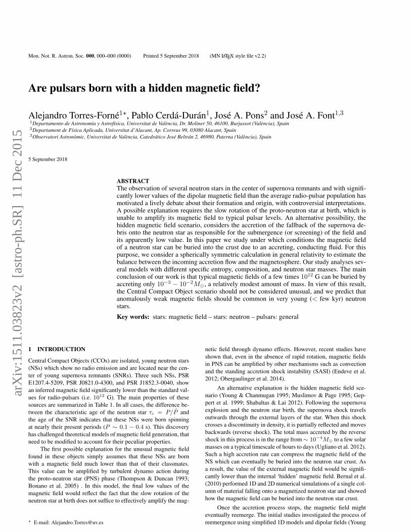
solve the Grad-Shafranov equation. We can obtain the field distri-bution after the compression by simply changing the radius wherethe boundary conditions are imposed. The evolution of the mag-netic field geometry before and after compression is shown in Fig. 3for three illustrative cases.

For the interior magnetic field, which determines the boundaryconditions at the surface of the star, we use two different magneticfield distributions, a dipolar magnetic field (dipole herafter) and apoloidal field generated by a circular loop of radius r = 4 × 105

cm (Jackson 1962) (loop current hereafter). Following Gabler et al(2012), it is useful to introduce the equivalent magnetic field, B∗,which we define as the magnetic field strength at the surface of aNewtonian, uniformly magnetized sphere with radius 10 km havingthe same dipole magnetic moment as the configuration we want todescribe. It spans the range B∗ ∈ [1010 − 1016] G.

5.2 Magnetosphere compression

In the case of a fluid accreting onto a force-free magnetosphere, themagnetopause will remain spherical and will move inwards as longas the total pressure of the unmagnetized fluid, ptot = p+pram , ex-ceeds that of the magnetic pressure, pmag, of the magnetosphere. Ifwe approximate the magnetopause as a spherical boundary betweenthe spherically symmetric accreting solution described in Section 3and the potential solution computed in Section 5.1, its propertiescan be described as the solution of a Riemann problem at the mag-netopause. Since the magnetic field of the initial state is tangentialto the magnetopause, we can use the exact solution of the Riemannproblem developed by Romero et al. (2005). A succinct summaryof the details of the implementation of the Riemann solver can befound in Appendix A.

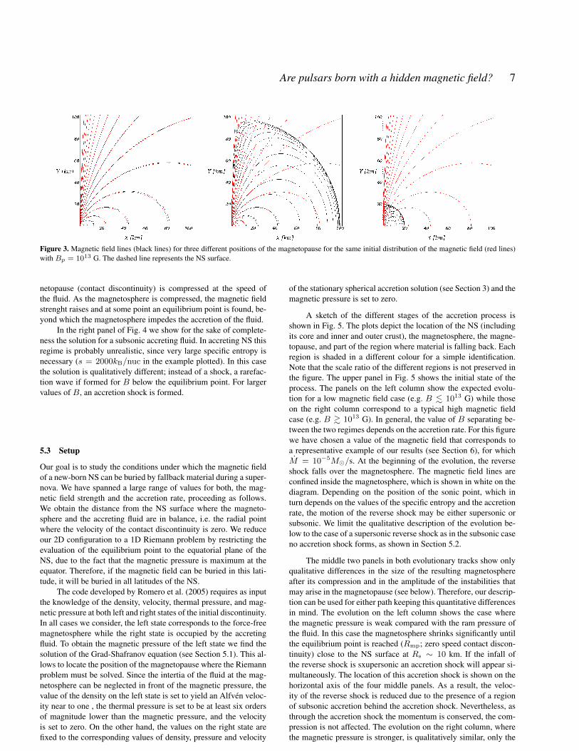
For illustrative purposes the left panel of Fig. 4 shows the so-lution of the Riemann problem for a supersonic fluid accreting fromthe right into a magnetically dominated region (magnetosphere) onthe left. The figure displays both the density (left axis, solid lines)and the fluid velocity (right axis, dashed lines). The initial discon-tinuity is located at x = 0. The right constant state of the Rie-mann problem corresponds to the accreting fluid with an entropyof s = 10 kB/nuc and accretion rate of M = 10−7 M�/s. Theleft constant state corresponds a state with magnetic pressureB2/2.The figure plots the corresponding solutions for different values ofB around the equilibrium (indicated in the legend).

Looking at the left panel of Fig. 4 from left to right, the firstjump in density corresponds to the contact discontinuity, point atwhich, as expected, the velocity remains continuos. The next dis-continuity is a shock wave, where both the density and veloc-ity are discontinuous, and both decrease. For low magnetic fields,B 6 1010G, the low magnetic pressure on the left state cannotcounteract the total pressure of the accreting fluid and the contactdiscontinuity advances to the right at a velocity equal to that ofthe accreting fluid; a shock front is practically nonexistent. As themagnetic field is increased the velocity of the contact discontinuitydecreases and it becomes zero at about B = 1013 G. We iden-tify this point as the equilibrium point, since no net flux of mattercrosses x = 0. Around this equilibrium point, an accretion shockappears, which heats and decelerates matter coming from the right.The equilibrium point corresponds to a solution in which the mattercrossing the shock has zero velocity, i.e. it piles up on top of the leftstate as the shock progresses to the right.

The actual accretion of matter onto a magnetically dominatedmagnetosphere is expected to behave in a similar way as the de-scribed Riemann problem. At large distances (low B) the mag-

© 0000 RAS, MNRAS 000, 000–000


Figure 3. Magnetic field lines (black lines) for three different positions of the magnetopause for the same initial distribution of the magnetic field (red lines)with Bp = 1013 G. The dashed line represents the NS surface.

netopause (contact discontinuity) is compressed at the speed ofthe fluid. As the magnetosphere is compressed, the magnetic fieldstrenght raises and at some point an equilibrium point is found, be-yond which the magnetosphere impedes the accretion of the fluid.

In the right panel of Fig. 4 we show for the sake of complete-ness the solution for a subsonic accreting fluid. In accreting NS thisregime is probably unrealistic, since very large specific entropy isnecessary (s = 2000kB/nuc in the example plotted). In this casethe solution is qualitatively different; instead of a shock, a rarefac-tion wave if formed for B below the equilibrium point. For largervalues of B, an accretion shock is formed.

5.3 Setup

Our goal is to study the conditions under which the magnetic fieldof a new-born NS can be buried by fallback material during a super-nova. We have spanned a large range of values for both, the mag-netic field strength and the accretion rate, proceeding as follows.We obtain the distance from the NS surface where the magneto-sphere and the accreting fluid are in balance, i.e. the radial pointwhere the velocity of the contact discontinuity is zero. We reduceour 2D configuration to a 1D Riemann problem by restricting theevaluation of the equilibrium point to the equatorial plane of theNS, due to the fact that the magnetic pressure is maximum at theequator. Therefore, if the magnetic field can be buried in this lati-tude, it will be buried in all latitudes of the NS.

The code developed by Romero et al. (2005) requires as inputthe knowledge of the density, velocity, thermal pressure, and mag-netic pressure at both left and right states of the initial discontinuity.In all cases we consider, the left state corresponds to the force-freemagnetosphere while the right state is occupied by the accretingfluid. To obtain the magnetic pressure of the left state we find thesolution of the Grad-Shafranov equation (see Section 5.1). This al-lows to locate the position of the magnetopause where the Riemannproblem must be solved. Since the intertia of the fluid at the mag-netosphere can be neglected in front of the magnetic pressure, thevalue of the density on the left state is set to yield an Alfvén veloc-ity near to one , the thermal pressure is set to be at least six ordersof magnitude lower than the magnetic pressure, and the velocityis set to zero. On the other hand, the values on the right state arefixed to the corresponding values of density, pressure and velocity

of the stationary spherical accretion solution (see Section 3) and themagnetic pressure is set to zero.

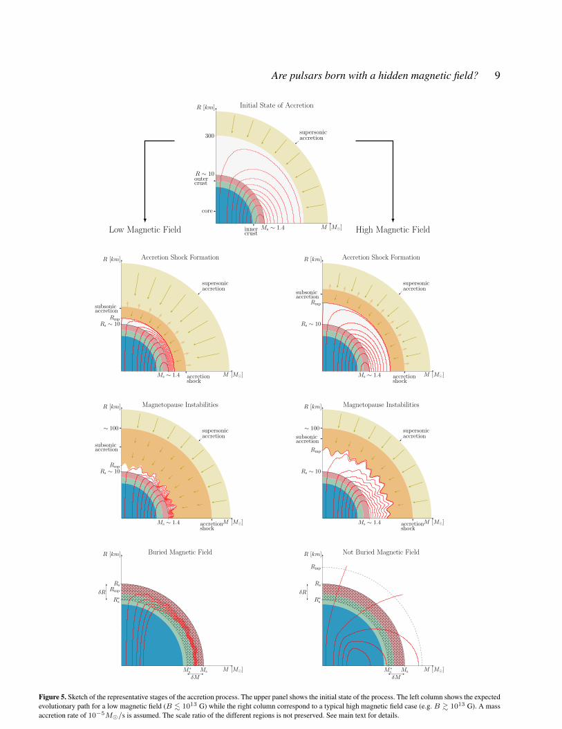
A sketch of the different stages of the accretion process isshown in Fig. 5. The plots depict the location of the NS (includingits core and inner and outer crust), the magnetosphere, the magne-topause, and part of the region where material is falling back. Eachregion is shaded in a different colour for a simple identification.Note that the scale ratio of the different regions is not preserved inthe figure. The upper panel in Fig. 5 shows the initial state of theprocess. The panels on the left column show the expected evolu-tion for a low magnetic field case (e.g. B . 1013 G) while thoseon the right column correspond to a typical high magnetic fieldcase (e.g. B & 1013 G). In general, the value of B separating be-tween the two regimes depends on the accretion rate. For this figurewe have chosen a value of the magnetic field that corresponds toa representative example of our results (see Section 6), for whichM = 10−5M�/s. At the beginning of the evolution, the reverseshock falls over the magnetosphere. The magnetic field lines areconfined inside the magnetosphere, which is shown in white on thediagram. Depending on the position of the sonic point, which inturn depends on the values of the specific entropy and the accretionrate, the motion of the reverse shock may be either supersonic orsubsonic. We limit the qualitative description of the evolution be-low to the case of a supersonic reverse shock as in the subsonic caseno accretion shock forms, as shown in Section 5.2.

The middle two panels in both evolutionary tracks show onlyqualitative differences in the size of the resulting magnetosphereafter its compression and in the amplitude of the instabilities thatmay arise in the magnetopause (see below). Therefore, our descrip-tion can be used for either path keeping this quantitative differencesin mind. The evolution on the left column shows the case wherethe magnetic pressure is weak compared with the ram pressure ofthe fluid. In this case the magnetosphere shrinks significantly untilthe equilibrium point is reached (Rmp; zero speed contact discon-tinuity) close to the NS surface at Rs ∼ 10 km. If the infall ofthe reverse shock is sxupersonic an accretion shock will appear si-multaneously. The location of this accretion shock is shown on thehorizontal axis of the four middle panels. As a result, the veloc-ity of the reverse shock is reduced due to the presence of a regionof subsonic accretion behind the accretion shock. Nevertheless, asthrough the accretion shock the momentum is conserved, the com-pression is not affected. The evolution on the right column, wherethe magnetic pressure is stronger, is qualitatively similar, only the

© 0000 RAS, MNRAS 000, 000–000


0.3 0.2 0.1 0.0 0.1 0.2 0.3

x

10−3

10−3

10−2

10−1

100

101

ρ [

g/cm

3]

B=1011 G

B=1012 G

B=5×1012 G

B=1013 G

0.5

0.0

0.5

1.0

v [c

]

0.3 0.2 0.1 0.0 0.1 0.2 0.3

x

10−3

10−3

10−2

10−1

100

101

102

103

104

105

ρ [

g/cm

3]

B=1011 G

B=1012 G

B=5×1012 G

B=1013 G

0.5

0.0

0.5

1.0

v [c

]

Figure 4. Density (solid lines, left axis) and velocity (dashed lines, right axis) profiles of the solution of the Riemann problem for several values of the magneticfield. Initially the discontinuity is set at x = 0, an accreting fluid at x > 0 and a magnetized fluid at x < 0, with constant magnetic field B. The left panelshows the case of supersonic accretion of a fluid with specific entropy s = 10kB/nuc and M = 10−7 M�/s at t = 0.3 s . The right panel shows the caseof subsonic accretion of a fluid with s = 2000kB/nuc and M = 10−5 M�/s at t = 0.3 s.

accretion shock is located further away from the NS surface and themagnetosphere is not so deeply compressed.

As we will discuss below in more detail, the compressionphase is unstable against the growth of Rayleigh-Taylor instabili-ties and the development of convection on the dynamic timescale.Therefore, the fluid and the magnetic field lines can mix, whichprovides a mechanism for the infalling fluid to actually reach thestar. As the fluid reaches the NS, the mass of the star grows fromM∗s to Ms and its radius increases from R∗s to Rs, encompassingthe twisted magnetic field lines a short distance away. The massaccreted δM forms part of the new crust of the NS, whose finalradius will depend on the total mass accreted during the process.The bottom panels of the diagram depict a magnified view of theNS to better visualize the rearrangement the mass of the star andthe magnetic field undergo. If the radius Rmp of the equilibriumpoint is lower than the new radius Rs, all the magnetic field lineswill be frozen inside the NS new crust, as shown in the bottom-leftplot of Fig. 5 which corresponds to the end of the accretion processfor a low magnetic field evolution. On the contrary, if the magneticfield is high, as considered on the evolutionary path on the right, theequilibrium point Rmp is far from the surface of the NS. Althoughpart of the infalling matter may still reach the star and form a newcrust, the mechanism is not as efficient as in the low magnetic fieldcase. This is depicted in the bottom-right panel of the figure.

In our approach, that we discuss in more detail in the sectionon results, we compare the distance obtained by the Riemann solverfor the location of Rmp (zero speed in the contact discontinuity)with the increment of the radius of the NS, δR, due to the pile up ofthe accreting matter. If the radial location of the equilibrium pointRmp is lower than δR (as in the bottom-left panel of Fig. 5) weconclude that the magnetic field is completely buried into the NScrust. On the contrary, if Rmp > δR, our approach does not allowus to draw any conclusion. In this case, multidimensional MHDnumerical simulations must be performed to obtain the final stateof the magnetic field.

6 RESULTS

We turn next to describe the main results of our study. In orderto be as comprehensive as possible, we cover a large number ofcases which are obtained from varying the physical parameters of

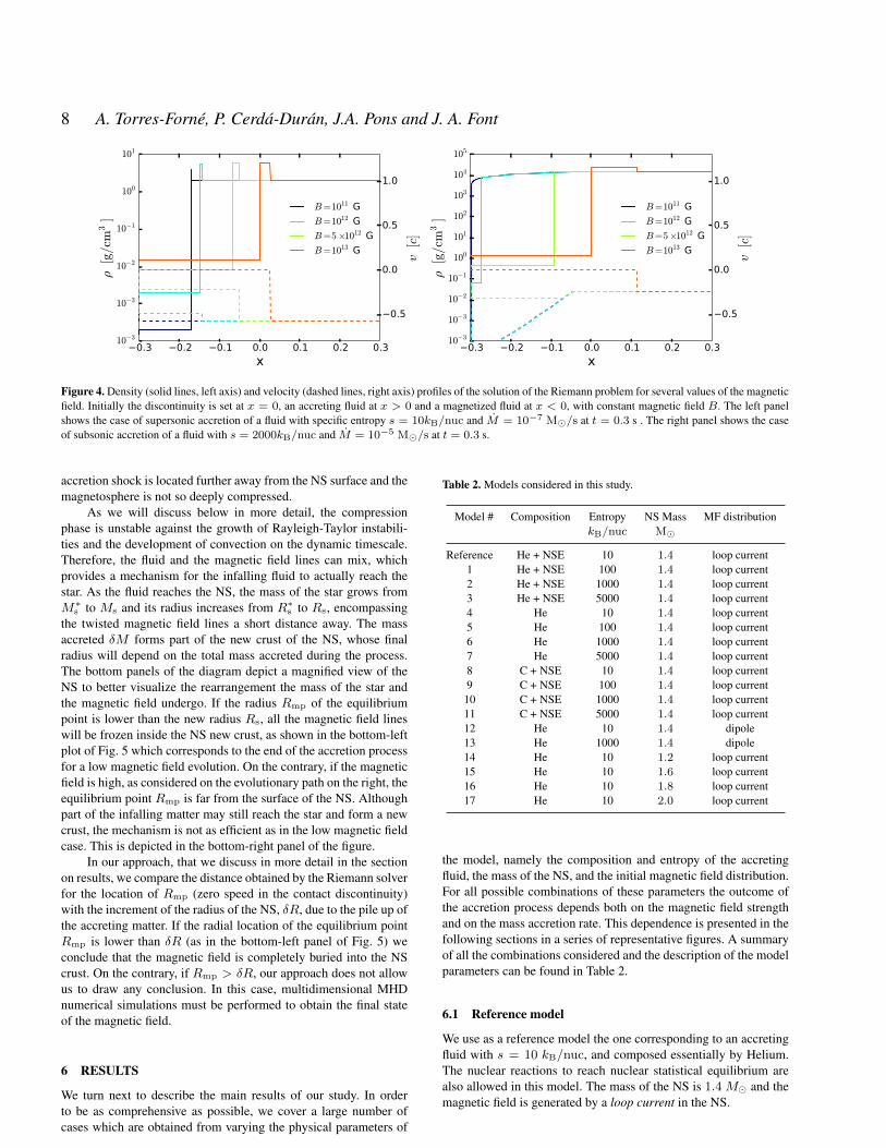
Table 2. Models considered in this study.

Model # Composition Entropy NS Mass MF distributionkB/nuc M�

Reference He + NSE 10 1.4 loop current1 He + NSE 100 1.4 loop current2 He + NSE 1000 1.4 loop current3 He + NSE 5000 1.4 loop current4 He 10 1.4 loop current5 He 100 1.4 loop current6 He 1000 1.4 loop current7 He 5000 1.4 loop current8 C + NSE 10 1.4 loop current9 C + NSE 100 1.4 loop current10 C + NSE 1000 1.4 loop current11 C + NSE 5000 1.4 loop current12 He 10 1.4 dipole13 He 1000 1.4 dipole14 He 10 1.2 loop current15 He 10 1.6 loop current16 He 10 1.8 loop current17 He 10 2.0 loop current

the model, namely the composition and entropy of the accretingfluid, the mass of the NS, and the initial magnetic field distribution.For all possible combinations of these parameters the outcome ofthe accretion process depends both on the magnetic field strengthand on the mass accretion rate. This dependence is presented in thefollowing sections in a series of representative figures. A summaryof all the combinations considered and the description of the modelparameters can be found in Table 2.

6.1 Reference model

We use as a reference model the one corresponding to an accretingfluid with s = 10 kB/nuc, and composed essentially by Helium.The nuclear reactions to reach nuclear statistical equilibrium arealso allowed in this model. The mass of the NS is 1.4 M� and themagnetic field is generated by a loop current in the NS.

© 0000 RAS, MNRAS 000, 000–000


Low Magnetic Field M [M�]

R [km]

Ms ∼ 1.4

300

R ∼ 10

core

outercrust

innercrust

supersonicaccretion

Initial State of Accretion

High Magnetic Field

M [M�]

R [km]

Ms ∼ 1.4

Rmp

Rs ∼ 10

supersonicaccretion

accretionshock

subsonicaccretion

Accretion Shock Formation

M [M�]

R [km]

Ms ∼ 1.4

Rmp

Rs ∼ 10

supersonicaccretion

accretionshock

subsonicaccretion

Accretion Shock Formation

M [M�]

R [km]

Ms ∼ 1.4

Rmp

Rs ∼ 10

supersonicaccretion

accretionshock

subsonicaccretion

∼ 100

Magnetopause Instabilities

M [M�]

R [km]

Ms ∼ 1.4

Rmp

Rs ∼ 10

supersonicaccretion

accretionshock

subsonicaccretion

∼ 100

Magnetopause Instabilities

M [M�]

R [km]

MsM ∗s

Rmp

Rs

R∗s

δR

δMaccretionshock

subsonicaccretion

Buried Magnetic Field

M [M�]

R [km]

MsM ∗s

Rmp

Rs

R∗s

δR

δMaccretionshock

subsonicaccretion

Not Buried Magnetic Field

Figure 5. Sketch of the representative stages of the accretion process. The upper panel shows the initial state of the process. The left column shows the expectedevolutionary path for a low magnetic field (B . 1013 G) while the right column correspond to a typical high magnetic field case (e.g. B & 1013 G). A massaccretion rate of 10−5M�/s is assumed. The scale ratio of the different regions is not preserved. See main text for details.

© 0000 RAS, MNRAS 000, 000–000


10−5 10−4 10−3 10−2 10−1

δM [M¯]

104

105

106

107

108

109

1010

1011

δR [

cm]

supersonic accretion

outer crust

inner crust core

accretion shock

B ∗ =1010 G

B ∗ =1011 G

B ∗ =1012 G

B ∗ =1013 G

B ∗ =1014 G

B ∗ =1015 G

B ∗ =1016 G

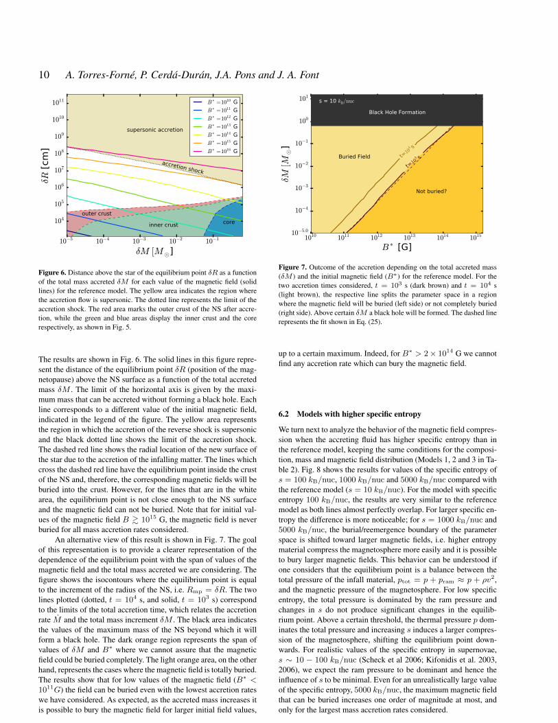
Figure 6. Distance above the star of the equilibrium point δR as a functionof the total mass accreted δM for each value of the magnetic field (solidlines) for the reference model. The yellow area indicates the region wherethe accretion flow is supersonic. The dotted line represents the limit of theaccretion shock. The red area marks the outer crust of the NS after accre-tion, while the green and blue areas display the inner crust and the corerespectively, as shown in Fig. 5.

The results are shown in Fig. 6. The solid lines in this figure repre-sent the distance of the equilibrium point δR (position of the mag-netopause) above the NS surface as a function of the total accretedmass δM . The limit of the horizontal axis is given by the maxi-mum mass that can be accreted without forming a black hole. Eachline corresponds to a different value of the initial magnetic field,indicated in the legend of the figure. The yellow area representsthe region in which the accretion of the reverse shock is supersonicand the black dotted line shows the limit of the accretion shock.The dashed red line shows the radial location of the new surface ofthe star due to the accretion of the infalling matter. The lines whichcross the dashed red line have the equilibrium point inside the crustof the NS and, therefore, the corresponding magnetic fields will beburied into the crust. However, for the lines that are in the whitearea, the equilibrium point is not close enough to the NS surfaceand the magnetic field can not be buried. Note that for initial val-ues of the magnetic field B & 1015 G, the magnetic field is neverburied for all mass accretion rates considered.

An alternative view of this result is shown in Fig. 7. The goalof this representation is to provide a clearer representation of thedependence of the equilibrium point with the span of values of themagnetic field and the total mass accreted we are considering. Thefigure shows the isocontours where the equilibrium point is equalto the increment of the radius of the NS, i.e. Rmp = δR. The twolines plotted (dotted, t = 104 s, and solid, t = 103 s) correspondto the limits of the total accretion time, which relates the accretionrate M and the total mass increment δM . The black area indicatesthe values of the maximum mass of the NS beyond which it willform a black hole. The dark orange region represents the span ofvalues of δM and B∗ where we cannot assure that the magneticfield could be buried completely. The light orange area, on the otherhand, represents the cases where the magnetic field is totally buried.The results show that for low values of the magnetic field (B∗ <1011G) the field can be buried even with the lowest accretion rateswe have considered. As expected, as the accreted mass increases itis possible to bury the magnetic field for larger initial field values,

1010 1011 1012 1013 1014 1015

B ∗ [G]

10−5.0

10−4

10−3

10−2

10−1

100

101

δM[M

¯]

s = 10 kB/nuc

Black Hole Formation

Buried Field

Not buried?

t=10

3 st=10

4 s

Figure 7. Outcome of the accretion depending on the total accreted mass(δM ) and the initial magnetic field (B∗) for the reference model. For thetwo accretion times considered, t = 103 s (dark brown) and t = 104 s(light brown), the respective line splits the parameter space in a regionwhere the magnetic field will be buried (left side) or not completely buried(right side). Above certain δM a black hole will be formed. The dashed linerepresents the fit shown in Eq. (25).

up to a certain maximum. Indeed, for B∗ > 2× 1014 G we cannotfind any accretion rate which can bury the magnetic field.

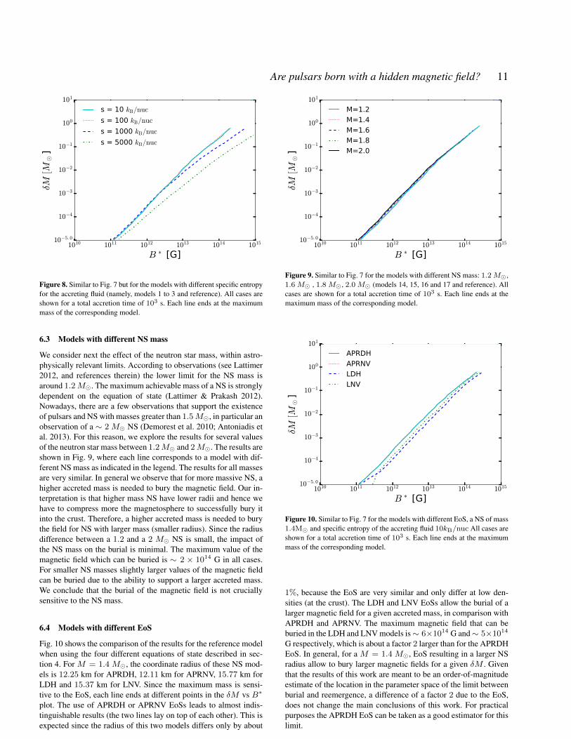
6.2 Models with higher specific entropy

We turn next to analyze the behavior of the magnetic field compres-sion when the accreting fluid has higher specific entropy than inthe reference model, keeping the same conditions for the composi-tion, mass and magnetic field distribution (Models 1, 2 and 3 in Ta-ble 2). Fig. 8 shows the results for values of the specific entropy ofs = 100 kB/nuc, 1000 kB/nuc and 5000 kB/nuc compared withthe reference model (s = 10 kB/nuc). For the model with specificentropy 100 kB/nuc, the results are very similar to the referencemodel as both lines almost perfectly overlap. For larger specific en-tropy the difference is more noticeable; for s = 1000 kB/nuc and5000 kB/nuc, the burial/reemergence boundary of the parameterspace is shifted toward larger magnetic fields, i.e. higher entropymaterial compress the magnetosphere more easily and it is possibleto bury larger magnetic fields. This behavior can be understood ifone considers that the equilibrium point is a balance between thetotal pressure of the infall material, ptot = p + pram ≈ p + ρv2,and the magnetic pressure of the magnetosphere. For low specificentropy, the total pressure is dominated by the ram pressure andchanges in s do not produce significant changes in the equilib-rium point. Above a certain threshold, the thermal pressure p dom-inates the total pressure and increasing s induces a larger compres-sion of the magnetosphere, shifting the equilibrium point down-wards. For realistic values of the specific entropy in supernovae,s ∼ 10 − 100 kB/nuc (Scheck et al 2006; Kifonidis et al. 2003,2006), we expect the ram pressure to be dominant and hence theinfluence of s to be minimal. Even for an unrealistically large valueof the specific entropy, 5000 kB/nuc, the maximum magnetic fieldthat can be buried increases one order of magnitude at most, andonly for the largest mass accretion rates considered.

© 0000 RAS, MNRAS 000, 000–000


1010 1011 1012 1013 1014 1015

B ∗ [G]

10−5. 0

10−4

10−3

10−2

10−1

100

101

δM[M

¯]

s = 10 kB/nuc

s = 100 kB/nuc

s = 1000 kB/nuc

s = 5000 kB/nuc

Figure 8. Similar to Fig. 7 but for the models with different specific entropyfor the accreting fluid (namely, models 1 to 3 and reference). All cases areshown for a total accretion time of 103 s. Each line ends at the maximummass of the corresponding model.

6.3 Models with different NS mass

We consider next the effect of the neutron star mass, within astro-physically relevant limits. According to observations (see Lattimer2012, and references therein) the lower limit for the NS mass isaround 1.2M�. The maximum achievable mass of a NS is stronglydependent on the equation of state (Lattimer & Prakash 2012).Nowadays, there are a few observations that support the existenceof pulsars and NS with masses greater than 1.5M�, in particular anobservation of a ∼ 2 M� NS (Demorest et al. 2010; Antoniadis etal. 2013). For this reason, we explore the results for several valuesof the neutron star mass between 1.2M� and 2M�. The results areshown in Fig. 9, where each line corresponds to a model with dif-ferent NS mass as indicated in the legend. The results for all massesare very similar. In general we observe that for more massive NS, ahigher accreted mass is needed to bury the magnetic field. Our in-terpretation is that higher mass NS have lower radii and hence wehave to compress more the magnetosphere to successfully bury itinto the crust. Therefore, a higher accreted mass is needed to burythe field for NS with larger mass (smaller radius). Since the radiusdifference between a 1.2 and a 2 M� NS is small, the impact ofthe NS mass on the burial is minimal. The maximum value of themagnetic field which can be buried is ∼ 2 × 1014 G in all cases.For smaller NS masses slightly larger values of the magnetic fieldcan be buried due to the ability to support a larger accreted mass.We conclude that the burial of the magnetic field is not cruciallysensitive to the NS mass.

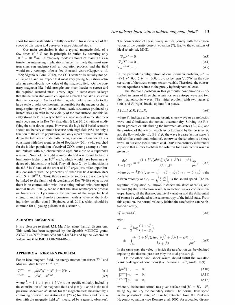
6.4 Models with different EoS

Fig. 10 shows the comparison of the results for the reference modelwhen using the four different equations of state described in sec-tion 4. For M = 1.4 M�, the coordinate radius of these NS mod-els is 12.25 km for APRDH, 12.11 km for APRNV, 15.77 km forLDH and 15.37 km for LNV. Since the maximum mass is sensi-tive to the EoS, each line ends at different points in the δM vs B∗

plot. The use of APRDH or APRNV EoSs leads to almost indis-tinguishable results (the two lines lay on top of each other). This isexpected since the radius of this two models differs only by about

1010 1011 1012 1013 1014 1015

B ∗ [G]

10−5. 0

10−4

10−3

10−2

10−1

100

101

δM[M

¯]

M=1.2

M=1.4

M=1.6

M=1.8

M=2.0

Figure 9. Similar to Fig. 7 for the models with different NS mass: 1.2M�,1.6M� , 1.8M�, 2.0M� (models 14, 15, 16 and 17 and reference). Allcases are shown for a total accretion time of 103 s. Each line ends at themaximum mass of the corresponding model.

1010 1011 1012 1013 1014 1015

B ∗ [G]

10−5. 0

10−4

10−3

10−2

10−1

100

101

δM[M

¯]

APRDH

APRNV

LDH

LNV

Figure 10. Similar to Fig. 7 for the models with different EoS, a NS of mass1.4M� and specific entropy of the accreting fluid 10kB/nuc All cases areshown for a total accretion time of 103 s. Each line ends at the maximummass of the corresponding model.

1%, because the EoS are very similar and only differ at low den-sities (at the crust). The LDH and LNV EoSs allow the burial of alarger magnetic field for a given accreted mass, in comparison withAPRDH and APRNV. The maximum magnetic field that can beburied in the LDH and LNV models is∼ 6×1014 G and∼ 5×1014

G respectively, which is about a factor 2 larger than for the APRDHEoS. In general, for a M = 1.4 M�, EoS resulting in a larger NSradius allow to bury larger magnetic fields for a given δM . Giventhat the results of this work are meant to be an order-of-magnitudeestimate of the location in the parameter space of the limit betweenburial and reemergence, a difference of a factor 2 due to the EoS,does not change the main conclusions of this work. For practicalpurposes the APRDH EoS can be taken as a good estimator for thislimit.

© 0000 RAS, MNRAS 000, 000–000


6.5 Remaining models

We do not observe any significant differences with respect to thereference model in the results for the models with different initialcomposition of the reverse shock (models 8 to 11) or the ones us-ing the NSE calculations (models 4 to 7). As a result we do notpresent additional figures for these models since the limiting linesoverlap with those of the reference model. The observed lack ofdependence is due to the fact that the EoS only depends on theelectron fraction, Ye. This value is obtained from the ratio betweenthe mean atomic mass number (A) and the mean atomic number(Z). For both cases of pure Helium and pure Carbon, this ratio isequal to Ye = 0.5 and, consequently, the values of pressure anddensity for the accreting fluid are almost identical, producing dif-ferences in the results below the numerical error of our method 2.In the case of the NSE calculation, the reason is similar. For lowentropies (s = 10, 100 kB/nuc) the temperature is not sufficientlyhigh to start the nuclear reactions and the composition remains con-stant throughout the accretion phase. For higher entropies, althoughthe value of the electron fraction may differ from 0.5 during the ac-cretion process, the differences produced in the thermodynamicalvariables lead to changes in the results of the Riemann problemstill below the numerical error of the method.

Regarding the initial distribution of the magnetic field, we donot observe either any significant difference in the results in thetwo cases that we have considered, loop current and dipole. Giventhat we are comparing models with the same effective magneticfield, B∗, and thus the same magnetic dipolar moment, the mag-netic field is virtually identical at long radial distances and the onlydifferences appear close to the NS surface. In practice the magneticfield structure only changes the details of the burial in the cases inwhich the equilibrium point is close to the burial depth (the limitingline plotted in the Figs. 7 to 10), but it does not change the locationof the limit itself in a sensitive way. As a conclusion, we can saythat the dominant ingredient affecting the burial of the magneticfield is the presence of a dipolar component of the magnetic fieldbut, for order-of-magnitude estimations, a multipolar structure ofthe field is mostly irrelevant.

7 SUMMARY AND DISCUSSION

We have studied the process of submergence of magnetic field ina newly born neutron star during a hypercritical accretion stage incoincidence with core collapse supernovae explosions. This is oneof the possible scenarios proposed to explain the apparently lowexternal dipolar field of CCOs. Our approach is based on 1D solu-tions of the relativistic Riemann problem, which provide the loca-tion of the spherical boundary (magnetopause) matching an exter-nal non-magnetised accretion solution with an internal magneticfield potential solution. For a given accretion rate and magneticfield strength, the magnetopause keeps moving inwards if the total(matter plus ram) pressure of the accreting fluid, exceeds the mag-netic pressure below the magnetopause. Exploring a wide range ofaccretion rates and field strengths, we have found the conditions forthe magnetopause to reach the equilibrium point below the NS sur-face, which implies the burial of the magnetic field. Our study hasconsidered several models with different specific entropy, composi-tion, and neutron star masses. Assuming an accretion time of 1000s,

2 The numerical error is dominated by the calculation of the equilibriumpoint, which is computed with a relative accuracy of 10−4.

our findings can be summarised by a general condition, rather in-dependent on the model details, relating the required total accretedmass to bury the magnetic field with the field strength. An approx-imate fit is (see dashed line in Fig. 7)

δM

M�≈(

B

2.5× 1014

)2/3

. (25)

The most important caveat in our approach is that we are re-stricted to a simplistic 1D spherical geometry, which does not allowus to consistently account for the effect of different MHD instabil-ities that can modify the results. We also note that our scenario isquite different from the extensively studied case of X-ray binaries,in which the NS accretes matter from a companion but at muchlower rates (sub-Eddington) and matter is mostly transparent to ra-diation during accretion. In that case, matter cools down throughX-ray emission during the accretion process. Davidson & Ostriker(1973) and Lamb (1973) already noticed this fact and predicted thatthe accretion will most likely be channeled through the magneticpoles, in analogy to the Earth’s magnetosphere. In the context ofX-ray binaries, Arons & Lea (1976) and Michel (1977) were ableto compute equilibrium solutions with a deformed magnetosphereand a cusp like accretion region at the magnetic poles. However,as the same authors pointed out, these systems are unstable to theinterchange instability (Kruskal & Schwarzschild 1954), a Railegh-Taylor-like instabilitiy in which magnetic field flux tubes from themagnetosphere can raise, allowing the fluid to sink. This might al-low for the formation of bubbles of material that fall through themagnetosphere down to the NS surface. In the case of a fluid de-posited on top of a highly magnetized region, modes with any pos-sible wavelength will be unstable (Kruskal & Schwarzschild 1954),however, in practice these instabilities are limited to the size of themagnetosphere (∼ Rmp) in the angular direction. As the bubblesof accreted material sink, magnetic flux tubes raise, as long as theirmagnetic pressure equilibrates the ram pressure of the unmagne-tized accreting fluid (Arons & Lea 1976). Therefore, in a naturalway, the equilibrium radius computed in Section 5.2 roughly deter-mines the highest value at which the magnetic field can raise.

This accretion mechanism through instabilities has beenshown to work in the case of X-ray binaries in global 3D numer-ical simulations (e.g. Kulkarni & Romanova 2008; Romanova etal. 2008). In the case of the hypercritical accretion present in thesupernova fallback, Rayleigh-Taylor instabilities have been stud-ied by Payne & Melatos (2004, 2007); Bernal et al. (2010, 2013);Mukherjee et al (2013a,b). The simulations of Bernal et al. (2013)also show that the height of the unstable magnetic field over theNS surface decreases with increasing accretion rate, for fixed NSmagnetic field strength, as expected. Using the method describedin Section 5.2 we have estimated the equilibrium height over theNS surface for the 4 models presented in Fig. 9 of Bernal et al.(2013), for their lower accretion rates (M 6 10−6 M�/s). Ourresults predict correctly the order of magnitude of the extent of theunstable magnetic field over the NS surface. Therefore, our sim-ple 1D model for the equilibrium radius serves as a good estimatorof the radius confining the magnetic field during the accretion pro-cess, although details about the magnetic field structure cannot bepredicted. Another important difference with the binary scenariois the duration of the accretion process. In X-ray binaries, a lowaccretion rate is maintained over very long times, so that instabil-ities have always time to grow. In our case, hypercritical accretioncan last only hundreds or thousands of seconds, and depending onthe particular values of density and magnetic field, this may be too

© 0000 RAS, MNRAS 000, 000–000


short for some instabilities to fully develop. This issue is out of thescope of this paper and deserves a more detailed study.

Our main conclusion is that a typical magnetic field of afew times 1012 G can in principle be buried by accreting only10−3 − 10−2M�, a relatively modest amount of mass. This es-timate has interesting implications: since it is likely that most neu-tron stars can undergo such an accretion process, and the fieldwould only reemerge after a few thousand years (Geppert et al.1999; Viganò & Pons 2012), the CCO scenario is actually not pe-culiar at all and we expect that most very young NSs show actu-ally an anomalously low value of the magnetic field. On the con-trary, magnetar-like field strengths are much harder to screen andthe required accreted mass is very large, in some cases so largethat the neutron star would collapse to a black hole. We also stressthat the concept of burial of the magnetic field refers only to thelarge scale dipolar component, responsible for the magnetospherictorque spinning down the star. Small scale structures produced byinstabilities can exist in the vicinity of the star surface, and this lo-cally strong field is likely to have a visible imprint in the star ther-mal spectrum, as in Kes 79 (Shabaltas & Lai 2012), without modi-fying the spin-down torque. However, the high field burial scenarioshould not be very common because both, high field NSs are only afraction to the entire population, and only a part of them would un-dergo the fallback episode with the right amount of matter. This isconsistent with the recent results of Bogdanov (2014) who searchedfor the hidden population of evolved CCOs among a sample of nor-mal pulsars with old characteristic ages but close to a supernovaremnant. None of the eight sources studied was found to have aluminosity higher than 1033 erg/s, which would have been an evi-dence of a hidden strong field. They all show X-ray luminosities inthe 0.3-3 keV band of the order of 1031 erg/s (or similar upper lim-its), consistent with the properties of other low field neutron starswith B ≈ 1012 G. Thus, these sample of sources are not likely tobe linked to the family of descendants of Kes 79-like objects, butthere is no contradiction with these being pulsars with reemergednormal fields. Finally, we note that the slow reemergence processon timescales of kyrs mimics the increase of the magnetic fieldstrength, and it is therefore consistent with a value of the brak-ing index smaller than 3 (Espinoza et al. 2011), which should becommon for all young pulsars in this scenario.

ACKNOWLEDGMENTS

It is a pleasure to thank J.M. Martí for many fruitful discussions.This work has been supported by the Spanish MINECO grantsAYA2013-40979-P and AYA2013-42184-P and by the GeneralitatValenciana (PROMETEOII-2014-069).

APPENDIX A: RIEMANN PROBLEM

For an ideal magneto-fluid, the energy-momentum tensor Tµν andMaxwell dual tensor F ∗µν are

Tµν = ρhuµuν + gµν p− bµbν , (A1)

F ∗µν = uµbν − uνbµ , (A2)

where h = 1 + ε + p/ρ + b2/ρ is the specific enthalpy includingthe contribution of the magnetic field and p = p+ b2/2 is the totalpressure. Moreover, bµ stands for the magnetic field measured by acomoving observer (see Antón et al. (2006) for details and its rela-tion with the magnetic field Bµ measured by a generic observer).

The conservation of these two quantities, jointly with the conser-vation of the density current, equation (7), lead to the equations ofideal relativistic MHD.

∇µJµ = 0 , (A3)

∇µTµν = 0 , (A4)

∇µF ∗µν = 0 . (A5)

In the particular configuration of our Riemann problem, uµ =W (1, vx, 0, vz), bµ = (0, 0, b, 0), so the term ∇µbµbν in the con-servation of the stress-energy tensor, vanish. Therefore, the conser-vation equations reduce to the purely hydrodynamical case.

The Riemann problem in this particular configuration is de-scribed in terms of three characteristics, one entropy wave and twofast magnetosonic waves. The initial problem with two states L(left) and R (right) breaks up into four states,

LW←L∗CR∗W→R, (A6)

whereW indicate a fast magnetosonic shock wave or a rarefactionwave and C indicates the contact discontinuity. Solving the Rie-mann problem entails finding the intermediate states (L∗, R∗) andthe position of the waves, which are determined by the pressure p∗and the flow velocity vx∗ . If p 6 p∗ the wave is a rarefaction wave (aself-similar continuous solution), otherwise the solution is a shockwave. In our case (see Romero et al. 2005) the ordinary differentialequation that allows to obtain the solution for a rarefaction wave isgiven by

dvx

1− (vx)2= ±

(1 + b2/(ρhcs))

√h+ A2(1− w2)

h2 + A2

dp

ρw, (A7)

where A = hWvz , w = c2s + v2A − c2sv2A, vA = b2/ρh is the

Alfvén velocity and cs =

√1h∂p∂ρ

∣∣∣s

is the sound speed. The in-

tegration of equation A7 allows to conect the states ahead (a) andbehind (b) the rarefaction wave. Rarefaction waves conserve en-tropy, hence, all the thermodynamical variables and the differentialof pmust be calculated at the same entropy of the initial state. Fromthis equation, the normal velocity behind the rarefaction can be ob-tained directly,

vxb = tanh C, (A8)

with

C =1

2log

(1 + vxa1− vxa

)

±∫ pb

pa

(1 + b2/(ρhcs))

√h+ A2(1− w2)

h2 + A2

dp

ρw. (A9)

In the same way, the velocity inside the rarefaction can be obtainedreplacing the thermal pressure p by the total pressure p.

On the other hand, shock waves should fulfill the so-calledRankine-Hugoniot conditions (Lichnerowicz 1967; Anile 1989)

[ρuµ]nµ = 0 , (A10)

[Tµν ]nν = 0 , (A11)

[F ∗µν ]nν = 0 , (A12)

where nµ is the unit normal to a given surface and [H] ≡ Ha−Hbbeing Ha and Hb the boundary values. The normal flow speedin the post-shock state, vxb , can be extracted from the Rankine-Hugoniot equations (see Romero et al. 2005, for a detailed discus-

© 0000 RAS, MNRAS 000, 000–000


sion),

vxb =

(haWav

xa +

Ws(pb − pa)

j

)(A13)

×(haWa + (pb − pa)

(Wsv

xa

j+

1

ρaWa

))−1

, (A14)

where Ws = 1√1−V 2

s

is the Lorentz factor of the shock,

V ±s =ρ2aW

2a v

xa ± |j|

√j2 + ρ2aW 2

a (1− vxa)2

ρ2aW 2a + j2

, (A15)

is the shock speed, and

j ≡WsρaWa(Vs − vxa) = WsρbWb(Vs − vxb ) , (A16)

is an invariant derived directly from the Rankine-Hugoniot jumpconditions. These expressions, together with the Lichnerowicz adi-abat,

[h2] =

(hbρb

+haρa

), (A17)

allows us to calculate the shock wave solution.

REFERENCES

Aguilera D., Pons J.A., Miralles J.A, 2008, A&A, 486, 255Akmal A., Pandharipande V. R., Ravenhall D. G., 1998, Phys.

Rev. C, 58, 1804Anile A.M.,1989,Relativistic Fluids and Magneto-Fluids; with

Applications in Astrophysics and Plasma Physics. CambridgeUniversity Press.

Antón L., Zanotti, O., Miralles, J.A., Martí, J.M., Ibáñez, J.M.,Font, J.A., Pons, J.A., 2006 ,ApJ, 637, 296

Antoniadis J. et al, 2013, Science, 340, 1233232Arons J. , Lea S. M., 1976, ApJ, 207, 914Bernal C.G., Lee W.H., Page D., 2010, RMAA, 46, 309Bernal C.G., Lee W.H., Page D., 2013, ApJ, 770, 106Bignami, G. F., Caraveo, P. A., De Luca, A., Mereghetti, S. 2003,

Nature, 423, 725Blondin J.M., 1986, ApJ, 308, 755Bogdanov S., Ng C.-Y. and Kaspi V. M., 2014, ApJL, 792, L36Bonanno A. et al., 2005, A&A, 440, 199Burrows, A., Lattimer, J.M. , 1986, ApJ, 307, 178Chevalier R.A. , 1989, ApJ, 346, 847Janka, H.-T., Langanke, K., Marek, A., Martínez-Pinedo, G.,

Mller, B., 2007, Phys. Rep., 442, 38Colgate S.A. , 1971, ApJ, 163, 221Davidson, K., Ostriker, J.P., 1973,ApJ 179, 585De Luca, A., Mereghetti, S., Caraveo, P. A., Moroni, M., Mignani,

R. P., Bignami, G. F. 2004, A&A, 418, 625Demorest P. B., Pennucci T., Ransom S. M., Roberts M. S.

E.,Hessels J. W. T., 2010,Nature, 467, 1081Douchin F., Haensel P., 2001, A&A, 380, 151Endeve E., Cardall C.Y., Budiardja R.D., Beck S.W. and Bejnood

A., 2012 ApJ., 751, 26 (28pp)Espinoza, C. M., Lyne, A. G., Kramer, M., Manchester, R. N., &

Kaspi, V. M. 2011, ApJL, 741, L13Faucher-Giguère, C.-A.; Kaspi, V. M., 2006, ApJ, 643, 332Fryer, C. L. , 2006, New Ast. Rev., 50, 492-495Geppert U., Page D., Zannias T., 1999, A&A, 345, 847Goldreich P., Julian W.H., 1969, ApJ, 157, 869Gotthelf, E. V., Halpern J.P., 2007, ApJL, 664, L35

Gotthelf E.V., Halpern J.P., Seward S.D., 2005, ApJL, 627, 390-96Gotthelf E. V., Halpern J.P., Alford, J., 2013, ApJ, 766, id. 58Goussard, J.-O.; Haensel, P.; Zdunik, J. L., 1998, A&A, 330, 1005Gullón, M.; Miralles, J. A.; Viganò, D.; Pons, J.A., 2014, MN-

RAS, 443, 1891Hammer N.J., Janka H.-Th., Müller E., 2010, ApJ, 714, 1371Halpern, J. P., Gotthelf, E. V., Camilo, F., Seward, F. D. 2007, ApJ,

665, 1304 (Paper 2)Halpern, J. P., Gotthelf, E. V., Camilo, F., Seward, F. D. 2010, ApJ,

709, 436Helfand D.J, Becker R.H., 1984, Nature, 307, 215Ho W.C.G., 2011, MNRAS, 414, 2567Houck J.C., Chevalier R.A., 1991, ApJ, 376, 234Hui, C. Y., Becker, W. 2006, A&A, 454, 543Jackson, J. D. 1962, Classical electrodynamics, New York: Wiley.Gabler M., Cerdá-Durán P., Font J.A., Müller E, Stergioulas N. ,

2012, MNRAS, 430, 1811Joggerst C.C, Almgren A., Woosley S.E.,2010, ApJ, 723, 353Kifonidis K., Plewa T., Janka H.Th., Müller E., 2003, A&A, 408,

621Kifonidis K., Plewa T., Scheck L., Janka H.Th., Müller E., 2006,

A&A, 453, 661Kruskal, M., Schwarzschild, M. 1954, Proc. R. Soc. A, 223,

348âAS360Kulkarni, A. K., Romanova, M. M., 2008, MNRAS, 386, 673Lattimer J., Prakash M., 2005, Phys. Rev. Lett. 94, 111101Lattimer J., 2012, Annual Review of Nuclear and Particle Physics,

Vol. 62, 485Lamb, F. K., Pethick, C. J., Pines, D. 1973, Astrophysical Journal,

184, 271Lichnerowicz A.,1967, Relativistic Hydrodynamics and Magneto-

hydrodynamics. Benjamin.Lorimer D. R., Kramer M., 2004, Handbook of Pulsar Astronomy,

Cambridge University Press.Mereghetti, S., De Luca, A., Caraveo, P. A., Becker, W., Mignani,

R., Bignami, G. F. 2002, ApJ, 581, 1280Michel F.C., 1972, Ap. Space Sci., 15, 153Michel F.C., 1977, ApJ, 214, 261Mukherjee, D., Bhattacharya, D., Mignone, A. 2013, ApJ, 430,

1976Mukherjee, D., Bhattacharya, D., Mignone, A. 2013, ApJ, 435,

718Muslimov A., Page D., 1995, ApJ , 440, L77Negele J. W., Vautherin D., 1973, Nuclear Physics A, 207, 298Obergaulinger M., Janka H.T., Aloy-Torás M. A., 2014, MNRAS,

445, 3169Pandharipande V. R., Smith R. A., 1975, Physics Letters B, 59, 15Page, D., Lattimer J.M., Prakash M., Steiner, A.W., 2004, ApJS,

155, 623Payne, D. J. B., Melatos, A. 2004, ApJ, 351, 569âAS584Payne, D. J. B., Melatos, A. 2007,ApJ, 376, 609âAS624Pons J.A., Geppert U., 2007, A&A, 470, 303Pons J.A., Miralles, J.A., Geppert U., 2009, A&A, 496, 207Pons J.A., Reddy S., Prakash M., Lattimer J.M., Miralles J.A.,

1999, ApJ, 513, 780Romanova M. M., Kulkarni A. K., Lovelace, Richard V. E, ApJL,

673, L171.Romero R., Martí J.M, Pons J.A., Ibáñez J.M., Miralles J.A.,

2005, J. Fluid Mech., 544, 323-338Seitenzahl R. et al., 2008, ApJ, 685, L129Seward, F. D., Slane, P. O., Smith, R. K., Sun, M. 2003, ApJ, 584,

414

© 0000 RAS, MNRAS 000, 000–000


Shabaltas N. Lai D., 2012, ApJ 748, 148Shapiro S.L., Teukolsky S.A., 2004, Black holes, white dwarfs and

NSs, Wiley-VCH.Scheck L., Kifonidis K., Janka H.-Th., Müller E., 2006, A&A 457,

963Swarztrauber, 1974, SIAM J. Numer. Anal. 11, 1136-1150Thompson C., Duncan R.C., 1993, ApJ, 408, 194Timmes F.X, 1999, ApJ Supp. ser., 124, 241-263Timmes F.X., Arnett D., 1999, ApJ Supp. Ser., 125, 277-294Timmes F.X., Swesty D., 2000, ApJ Supp. Ser., 126, 501-516Turolla R., Esposito P., 2013, Int. J. Mod. Phys., D, 22, 1330024Viganò D., Pons J.A., 2012, MNRAS, 425, 2487-2492Viganò D., Rea, N.; Pons, J. A.; Perna, R.; Aguilera, D. N.; Mi-

ralles, J. A., 2013, MNRAS, 434, 123Ugliano M., Janka H.T., Marek A., Arcones A., 2012, ApJ, 757,

69Woosley S.E., Weaver T.A., 1995, ApJ Supp. Ser, 101, 181Woosley S.E., Heger A., Weaver T.A., 2002, Rev. Mod. Phys., 74,

1015Wongwathanarat A., Müller E., Janka H.-Th., 2015, A&A, 577,

A48Young E.J., Chanmugan G., 1995, ApJ, 442, L53Zavlin V.E., Pavlov G.G., Sanwal D., Trumper J., 2000, ApJL,

540, L25Zhang W., Woosley S.E., Heger A., 2008, ApJ, 679, 639

© 0000 RAS, MNRAS 000, 000–000

are pulsars born with a hidden magnetic ﬁeld?

Documents