Area Under the Precision-Recall Curve:Point Estimates and Confidence Intervals

Kendrick Boyd1, Kevin H. Eng2, and C. David Page1

1 University of Wisconsin-Madison, Madison, WIboyd@cs.wisc.edu,page@biostat.wisc.edu

2 Roswell Park Cancer Institute, Buffalo, NY Kevin.Eng@RoswellPark.org

Abstract. The area under the precision-recall curve (AUCPR) is a sin-gle number summary of the information in the precision-recall (PR)curve. Similar to the receiver operating characteristic curve, the PR curvehas its own unique properties that make estimating its enclosed areachallenging. Besides a point estimate of the area, an interval estimate isoften required to express magnitude and uncertainty. In this paper weperform a computational analysis of common AUCPR estimators andtheir confidence intervals. We find both satisfactory estimates and in-valid procedures and we recommend two simple intervals that are robustto a variety of assumptions.

1 Introduction

Precision-recall (PR) curves, like the closely-related receiver operating character-istic (ROC) curves, are an evaluation tool for binary classification that allows thevisualization of performance at a range of thresholds. PR curves are increasinglyused in the machine learning community, particularly for imbalanced data setswhere one class is observed more frequently than the other class. On these im-balanced or skewed data sets, PR curves are a useful alternative to ROC curvesthat can highlight performance differences that are lost in ROC curves [1]. Be-sides visual inspection of a PR curve, algorithm assessment often uses the areaunder a PR curve (AUCPR) as a general measure of performance irrespectiveof any particular threshold or operating point (e.g., [2,3,4,5]).

Machine learning researchers build a PR curve by first plotting precision-recall pairs, or points, that are obtained using different thresholds on a proba-bilistic or other continuous-output classifier, in the same way an ROC curve isbuilt by plotting true/false positive rate pairs obtained using different thresh-olds. Davis and Goadrich [6] showed that for any fixed data set, and hence fixednumbers of actual positive and negative examples, points can be translated be-tween the two spaces. After plotting the points in PR space, we next seek to

H. Blockeel et al. (Eds.): ECML PKDD 2013, Part III, LNAI 8190, pp. 451-466,2013. c© Springer-Verlag Berlin Heidelberg 2013The final publication is available at http://link.springer.com/chapter/10.1007%2F978-3-642-40994-3_29

construct a curve and compute the AUCPR and to construct 95% (or other)confidence intervals (CIs) around the curve and the AUCPR.

However, the best method to construct the curve and calculate area is notreadily apparent. The PR points from a small data set are shown in Fig. 1. Ques-tions immediately arise about what to do with multiple points with the samex-value (recall), whether linear interpolation is appropriate, whether the maxi-mum precision for each recall are representative, if convex hulls should be usedas in ROC curves, and so on. There are at least four distinct methods (with sev-eral variations) that have been used in machine learning, statistics, and relatedareas to compute AUCPR, and four methods that have been used to constructCIs. The contribution of this paper is to discuss and analyze eight estimatorsand four CIs empirically. We provide evidence in favor of computing AUCPRusing the lower trapezoid, average precision, or interpolated median estimatorsand using binomial or logit CIs rather than other methods that include the morewidely-used (in machine learning) ten-fold cross-validation. The differences inresults using these approaches are most striking when data are highly skewed,which is exactly the case when PR curves are most preferred over ROC curves.

● ●

●

●

●

●

●

●

●●

●●

●●

●●●

●●●●●●●●

●●●●●

0.00

0.25

0.50

0.75

1.00

0.00 0.25 0.50 0.75 1.00recall

prec

isio

n

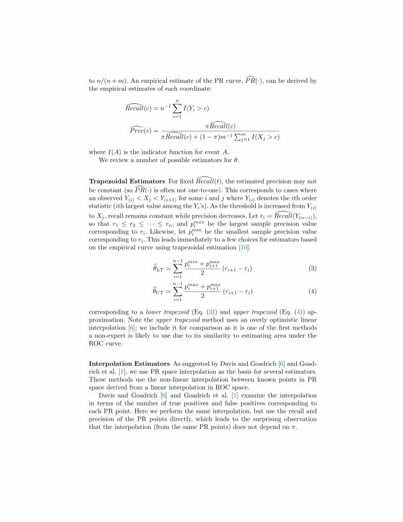
Fig. 1. Empirical PR points obtained froma small data set with 10 positive examplesand 20 negative examples.

Section 2 contains a review of PRcurves, Section 3 describes the esti-mators and CIs we evaluate, and Sec-tion 4 presents case studies of the es-timators and CIs in action.

2 Area Under thePrecision-Recall Curve

Consider a binary classification taskwhere models produce continuousoutputs, denoted Z, for each example.Diverse applications are subsumed bythis setup, e.g., a medical test to iden-tify diseased and disease-free patients,a document ranker to distinguish rele-vant and non-relevant documents to aquery, and generally any binary clas-sification task. The two categories areoften naturally labelled as positive(e.g., diseased, relevant) or negative (e.g., disease-free, non-relevant). Followingthe literature on ROC curves [7,8], we denote the output values for the negativeexamples by X and the output values for the positive examples by Y (Z is amixture of X and Y ). These populations are assumed to be independent whenthe class is known. Larger output values are associated with positive examples,so for a given threshold c, an example is predicted positive if its value is greaterthan c. We represent the category (or class) with the indicator variable D whereD = 1 corresponds to positive examples and D = 0 to negative examples. An

important aspect of a task or data set is the class skew π = P (D = 1). Skew isalso known as prevalence or a prior class distribution.

Several techniques exist to assess the performance of binary classificationacross a range of thresholds. While ROC analysis is the most common, we areinterested in the related PR curves. A PR curve may be defined as the set ofpoints:

PR(·) = {(Recall(c), P rec(c)),−∞ < c <∞}where Recall(c) = P (Y > c) and Prec(c) = P (D = 1|Z > c). Recall is equiva-lent to true positive rate or sensitivity (the y-axis in ROC curves), while precisionis the same as positive predictive value. Since larger output values are assumedto be associated with positive examples, as c decreases, Recall(c) increases toone and Prec(c) decreases to π. As c increases, Prec(c) reaches one as Recall(c)approaches zero under the condition that “the first document retrieved is rele-vant” [9]. In other words, whether the example with the largest output value ispositive or negative greatly changes the PR curve (approaching (0, 1) if positiveand (0, 0) if negative). Similarly, estimates of precision for recall near 0 tend tohave high variance, and this is a major difficulty in constructing PR curves.

It is often desirable to summarize the PR curve with a single scalar value.One summary is the area under the PR curve (AUCPR), which we will denoteθ. Following the work of Bamber [7] on ROC curves, AUCPR is an average ofthe precision weighted by the probability of a given threshold.

θ =

∫ ∞−∞

Prec(c)dP (Y ≤ c) (1)

=

∫ ∞−∞

P (D = 1|Z > c)dP (Y ≤ c). (2)

By Bayes’ rule and using that Z is a mixture of X and Y ,

P (D = 1|Z > c) =πP (Y > c)

πP (Y > c) + (1− π)P (X > c)

and we note that 0 ≤ θ ≤ 1 since Prec(c) and P (Y ≤ c) are bounded on the unitsquare. Therefore, θ might be viewed as a probability. If we consider Eq. (2) as animportance-sampled Monte Carlo integral, we may interpret θ as the fraction ofpositive examples among those examples whose output values exceed a randomlyselected c ∼ Y threshold.

3 AUCPR Estimators

In this section we summarize point estimators for θ and then introduce CI meth-ods.

3.1 Point Estimators

Let X1, . . . , Xm and Y1, . . . , Yn represent observed output values from negativeand positive examples, respectively. The skew π is assumed to be given or is set

to n/(n+m). An empirical estimate of the PR curve, PR(·), can be derived bythe empirical estimates of each coordinate:

Recall(c) = n−1n∑i=1

I(Yi > c)

P rec(c) =πRecall(c)

πRecall(c) + (1− π)m−1∑mj=1 I(Xj > c)

where I(A) is the indicator function for event A.We review a number of possible estimators for θ.

Trapezoidal Estimators For fixed Recall(t), the estimated precision may not

be constant (so PR(·) is often not one-to-one). This corresponds to cases wherean observed Y(i) < Xj < Y(i+1) for some i and j where Y(i) denotes the ith orderstatistic (ith largest value among the Yi’s). As the threshold is increased from Y(i)

to Xj , recall remains constant while precision decreases. Let ri = Recall(Y(n−i)),so that r1 ≤ r2 ≤ · · · ≤ rn, and pmaxi be the largest sample precision valuecorresponding to ri. Likewise, let pmini be the smallest sample precision valuecorresponding to ri. This leads immediately to a few choices for estimators basedon the empirical curve using trapezoidal estimation [10].

θLT =

n−1∑i=1

pmini + pmaxi+1

2(ri+1 − ri) (3)

θUT =

n−1∑i=1

pmaxi + pmaxi+1

2(ri+1 − ri) (4)

corresponding to a lower trapezoid (Eq. (3)) and upper trapezoid (Eq. (4)) ap-proximation. Note the upper trapezoid method uses an overly optimistic linearinterpolation [6]; we include it for comparison as it is one of the first methodsa non-expert is likely to use due to its similarity to estimating area under theROC curve.

Interpolation Estimators As suggested by Davis and Goadrich [6] and Goad-rich et al. [1], we use PR space interpolation as the basis for several estimators.These methods use the non-linear interpolation between known points in PRspace derived from a linear interpolation in ROC space.

Davis and Goadrich [6] and Goadrich et al. [1] examine the interpolationin terms of the number of true positives and false positives corresponding toeach PR point. Here we perform the same interpolation, but use the recall andprecision of the PR points directly, which leads to the surprising observationthat the interpolation (from the same PR points) does not depend on π.

Theorem 1. For two points in PR space (r1, p1) and (r2, p2) (assume WLOGr1 < r2), the interpolation for recall r′ with r1 ≤ r′ ≤ r2 is

p′ =r′

ar′ + b(5)

where

a = 1 +(1− p2)r2p2(r2 − r1)

− (1− p1)r1p1(r2 − r1)

b =(1− p1)r1

p1− (1− p2)r1r2

p2(r2 − r1)+

(1− p1)r21p1(r2 − r1)

Proof. First, we convert the points to ROC space. Let s1, s2 be the false posi-tive rates for the points (r1, p1) and (r2, p2), respectively. By definition of falsepositive rate,

si =(1− pi)πripi(1− π)

. (6)

A linear interpolation in ROC space for r1 ≤ r′ ≤ r2 has a false positive rate of

s′ = s1 +r′ − r1r2 − r1

(s2 − s1). (7)

Then convert back to PR space using

p′ =πr′

πr′ + (1− π)s′. (8)

Substituting Eq. (7) into Eq. (8) and using Eq. (6) for s1 and s2, we have

p′ = πr′[πr′ +

π(1− p1)r1p1

+π(r′ − r1)

r2 − r1

((1− p2)r2

p2− (1− p1)r1

p1

)]−1= r′

[r′(

1 +(1− p2)r2p2(r2 − r1)

− (1− p1)r1p1(r2 − r1)

)+

(1− p1)r1p1

− (1− p2)r1r2p2(r2 − r1)

+(1− p1)r21p1(r2 − r1)

]−1ut

Thus, despite PR space being sensitive to π and the translation to and fromROC space depending on π, the interpolation in PR space does not depend on π.One explanation is that each particular PR space point inherently contains theinformation about π, primarily in the precision value, and no extra knowledgeof π is required to perform the interpolation.

The area under the interpolated PR curve between these two points can becalculated analytically using the definite integral: 1∫ r2

r1

r′

ar′ + bdr′ =

ar′ − b log(ar′ + b)

a2

∣∣∣∣r′=r2r′=r1

=ar2 − b log(ar2 + b)− ar1 + b log(ar1 + b)

a2

1 Formula corrected from originally published version.

where a and b are defined as in Theorem 1.With the definite integral to calculate the area between two PR points, the

question is: which points should be used. The achievable PR curve of Davisof Goadrich [6] uses only those points (translated into PR space) that are onthe ROC convex hull. We also use three methods of summarizing from multiplePR points at the same recall to a single PR point to interpolate through. Thesummaries we use are the max, mean, and median of all pi for a particular ri.So we have four estimators using interpolation: convex, max, mean, and median.

Average precision Avoiding the empirical curve altogether, a plug-in estimateof θ, known in information retrieval as average precision [11], is:

θA =1

n

n∑i=1

P rec(Yi) (9)

which replaces the distribution function P (Y ≤ c) in Eq. (2) with its empiricalcumulative distribution function.

Binormal Estimator Conversely, a fully parametric estimator may be con-structed by assuming that Xj ∼ N (µx, σ

2x) and Yj ∼ N (µy, σ

2y). In this binormal

model [12], the MLE of θ is

θB =

∫ 1

0

πt

πt+ (1− π)Φ(µy−µx

σx+

σy

σxΦ−1(t)

) dt (10)

where µx, σx, µy, σy are sample means and variances of X and Y and Φ(t) is thestandard normal cumulative distribution function.

3.2 Confidence Interval Estimation

Having discussed AUCPR estimators, we now turn our attention to computingconfidence intervals (CIs) for these estimators. Our goal is to determine a simple,accurate interval estimate that is logistically easy to implement. We will comparetwo computationally intensive methods against two simple statistical intervals.

Bootstrap Procedure A common approach is to use a bootstrap procedure toestimate the variation in the data and to either extend a symmetric, normal-based interval about the point estimate or to take the empirical quantiles fromresampled data as interval bounds [13]. Because the relationship between thenumber of positive examples n and negative examples m is crucial for estimatingPR points and hence curves, we recommend using stratified bootstrap so π ispreserved exactly in all replicates. In our simulations we chose to use empiricalquantiles for the interval bounds and perform 1000 bootstrap replicates.

Cross-Validation Procedure Similarly, a cross-validation approach is a whollydata driven method for simultaneously producing the train/test splits requiredfor unbiased estimation of future performance and producing variance estimates.In k-fold cross-validation, the available data are partitioned into k folds. k − 1folds are used for training while the remaining fold is used for testing. By per-forming evaluation on the results of each fold separately, k estimates of perfor-mance are obtained. A normal approximation of the interval can be constructedusing the mean and variance of the k estimates. For more details and discussionof k-fold cross-validation, see Dietterich [14]. For our case studies we use thestandard k = 10.

Binomial Interval Recalling that 0 ≤ θ ≤ 1, we may interpret θ as a prob-ability associated with some binomial(1, θ) variable. If so, a CI for θ can beconstructed through the standard normal approximation:

θ ± Φ1−α/2

√θ(1− θ)

n

We use n for the sample size as opposed to n+m because n specifies the (max-

imum) number of unique recall values in PR(·). The binomial method can be

applied to any θ estimate once it is derived. A weakness of this estimate is thatit may produce bounds outside of [0, 1], even though 0 ≤ θ ≤ 1.

Logit Interval To obtain an interval which is guaranteed to produce endpoints

in [0, 1], we may use the logistic transformation η = log θ(1−θ)

where τ = s.e.(η) =

(nθ(1− θ))−1/2 by the delta method [15].On the logistic scale, an interval for η is η±Φ1−a/2τ . This can be converted

pointwise to produce an asymmetric logit interval bounded in [0, 1]:[eη−Φ(1−α/2)τ

1 + eη−Φ(1−α/2)τ,

eη+Φ(1−α/2)τ

1 + eη+Φ(1−α/2)τ

].

4 Case Studies

We use simulated data to evaluate the merits of the candidate point and intervalestimates discussed in Section 3 with the goal of selecting a subset of desirableprocedures. 2 The ideal point estimate would be unbiased, robust to variousdistributional assumptions on X and Y , and have good convergence as n + mincreases. A CI should have appropriate coverage, and smaller widths of theinterval are preferred over larger widths.

2 R code for the estimators and simulations may be found at http://pages.cs.wisc.edu/~boyd/projects/2013ecml_aucprestimation/

binormal bibeta offset uniform

−2 0 2 4 0.0 0.4 0.8 0.0 0.5 1.0 1.5c

dens

ity

X Y

Fig. 2. Probability density functions for X (negative) and Y (positive) output valuesfor binormal (X ∼ N(0, 1), Y ∼ N(1, 1)), bibeta (X ∼ B(2, 5), Y ∼ B(5, 2)), and offsetuniform (X ∼ U(0, 1), Y ∼ U(0.5, 1.5)) case studies.

We consider three scenarios for generating output values X and Y . Ourintention is to cover representative but not exhaustive cases whose conclusionswill be relevant generally. The densities for these scenarios are plotted in Fig. 2.The true PR curves (calculated using the cumulative distribution functions ofX and Y ) for π = 0.1 are shown in Fig. 3. Fig. 3 also contains sample empiricalPR curves that result from drawing data from X and Y . These are the curvesthe estimators work from, attempting to recover the area under the true curveas accurately as possible.

For unbounded continuous outputs, the binormal scenario assumes that X ∼N (0, 1) and Y ∼ N (µ, 1) where µ > 0. The distance between the two normaldistributions, µ, controls the discriminative ability of the assumed model. Fortest values bounded on [0, 1] (such as probability outputs), we replace the normaldistribution with a beta distribution. So the bibeta scenario has X ∼ B(a, b) andY ∼ B(b, a) where 0 < a < b. The larger the ratio between a and b, the betterable to distinguish between positive and negative examples. Finally, we modelan extreme scenario where the support of X and Y is not the same. This offsetuniform scenario is given by X ∼ U(0, 1) and Y ∼ U(γ, 1 + γ) for γ ≥ 0: thatis X lies uniformly on (0, 1) while Y is bounded on (γ, γ + 1). If γ = 0 there isno ability to discriminate, while γ > 1 leads to perfect classification of positiveand negative examples with a threshold of c = 1. All results in this paper useµ = 1, a = 2, b = 5, and γ = 0.5. These were chosen as representative examplesof the distributions that produce reasonable PR curves.

This paper exclusively uses simulated data drawn from specific, known dis-tributions because this allows calculation of the true PR curve (shown in Fig. 3)and the true AUCPR. Thus, we have a target value to compare the estimatesagainst and are able to evaluate the bias of an estimator and the coverage of aCI. This would be difficult to impossible if we used a model’s predictions on realdata because the true PR curve and AUCPR are unknown.

binormal bibeta offset uniform

0.00

0.25

0.50

0.75

1.00

0.00 0.25 0.50 0.75 1.00 0.00 0.25 0.50 0.75 1.00 0.00 0.25 0.50 0.75 1.00recall

prec

isio

n

Sample Curve True Curve

Fig. 3. True PR curves (calculated from the theoretical density functions) and sampledempirical PR curves, both at π = 0.1. Sampled PR curves use n + m = 500. Thesampled PR curves were generated by connecting PR points corresponding to adjacentthresholds values.

4.1 Bias and Robustness in Point Estimates

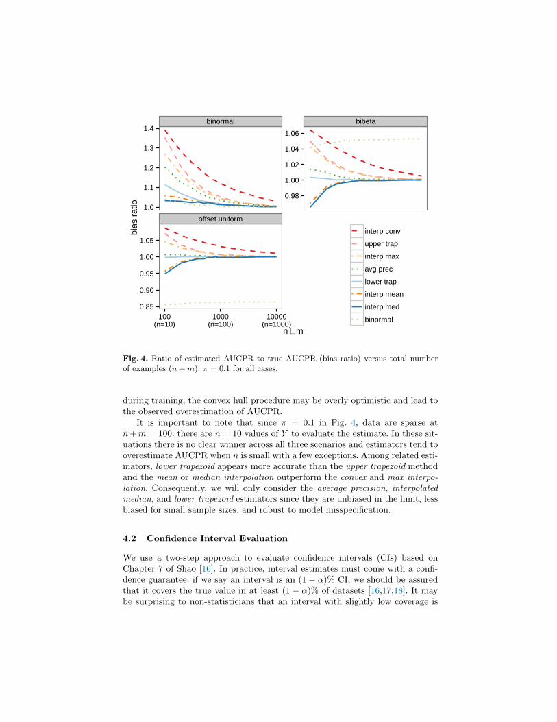
For each scenario, we evaluate eight estimators: the non-parametric average pre-cision, the parametric binormal, two trapezoidal estimates, and four interpolatedestimates. Fig. 4 shows the bias ratio versus n + m where π = 0.1 over 10,000simulations, and Fig. 5 shows the bias ratio versus π where n+m = 1000. Thebias ratio is the mean estimated AUCPR divided by the true AUCPR, so an un-biased estimator has a bias ratio of 1.0. Good point estimates of AUCPR shouldbe unbiased as n+m and π increase. That is, an estimator should have an ex-pected value equal to the true AUCPR (calculated by numerically integratingEq. 2).

As n+m grows large, most estimators converge to the true AUCPR in everycase. However, the binormal estimator shows the effect of model misspecification.When the data are truly binormal, it shows excellent performance but when thedata are bibeta or offset uniform, the binormal estimator converges to the wrongvalue. Interestingly, the bias due to misspecification that we observe for thebinormal estimate is lessened as the data become more balanced (π increases).

The interpolated convex estimate consistently overestimates AUCPR and ap-pears far from the true value even at n+m = 10000. The poor performance ofthe interpolated convex estimator seems surprising given how it uses the popu-lar convex hull ROC curve and then converts to PR space. Because the otherinterpolated estimators perform adequately, the problem may lie in evaluatingthe convex hull in ROC space. The convex hull chooses those particular pointsthat give the best performance on the test set. Analogous to using the test set

binormal bibeta

offset uniform

1.0

1.1

1.2

1.3

1.4

0.98

1.00

1.02

1.04

1.06

0.85

0.90

0.95

1.00

1.05

100(n=10)

1000(n=100)

10000(n=1000)

n + m

bias

rat

io

interp conv

upper trap

interp max

avg prec

lower trap

interp mean

interp med

binormal

Fig. 4. Ratio of estimated AUCPR to true AUCPR (bias ratio) versus total numberof examples (n+m). π = 0.1 for all cases.

during training, the convex hull procedure may be overly optimistic and lead tothe observed overestimation of AUCPR.

It is important to note that since π = 0.1 in Fig. 4, data are sparse atn+m = 100: there are n = 10 values of Y to evaluate the estimate. In these sit-uations there is no clear winner across all three scenarios and estimators tend tooverestimate AUCPR when n is small with a few exceptions. Among related esti-mators, lower trapezoid appears more accurate than the upper trapezoid methodand the mean or median interpolation outperform the convex and max interpo-lation. Consequently, we will only consider the average precision, interpolatedmedian, and lower trapezoid estimators since they are unbiased in the limit, lessbiased for small sample sizes, and robust to model misspecification.

4.2 Confidence Interval Evaluation

We use a two-step approach to evaluate confidence intervals (CIs) based onChapter 7 of Shao [16]. In practice, interval estimates must come with a confi-dence guarantee: if we say an interval is an (1 − α)% CI, we should be assuredthat it covers the true value in at least (1 − α)% of datasets [16,17,18]. It maybe surprising to non-statisticians that an interval with slightly low coverage is

binormal bibeta

offset uniform

2

4

6

0.8

1.0

1.2

0.25

0.50

0.75

1.00

0.01(n=10)

0.1(n=100)

0.5(n=500)

π

bias

rat

io

interp conv

upper trap

interp max

avg prec

lower trap

interp mean

interp med

binormal

Fig. 5. Ratio of estimated AUCPR to true AUCPR (bias ratio) versus π. In all casesn+m = 1000.

ruled inadmissible, but this would invalidate the guarantee. Additionally, target-ing an exact (1 − α)% interval is often impractical for technical reasons, hencethe at least (1−α)%. When an interval provides at least (1−α)% coverage, it isconsidered a valid interval and this is the first criteria a potential interval mustsatisfy.

After identifying valid methods for CIs, the second step is that we prefer thenarrowest (or optimal) intervals among the valid methods. The trivial [−∞,+∞]interval is a valid 95% CI because it always has at least 95% coverage (indeed,it has 100% coverage), but it conveys no useful information about the estimate.Thus we seek methods that produce the narrowest, valid intervals.

CI Coverage The first step in CI evaluation is to identify valid CIs with cov-erage at least (1 − α)%. In Fig. 6, we show results over 10,000 simulations forthe coverage of the four CI methods described in 3.2. These are 95% CIs, so thetarget coverage of 0.95 is denoted by the thick black line. As mentioned at theend of Section 4.1, we only consider the average precision, interpolated median,and lower trapezoid estimators for our CI evaluation.

A strong pattern emerges from Fig. 6 where the bootstrap and cross-validationintervals tend to have coverage below 0.95, though asymptotically approaching

●

●

●

●●

●

●

● ●

●

●

●●

●

●

● ●

●

●

● ●

●

●

●

● ●

●

●

●

●

●

●

●

●●

●

●

●●

●

●

● ●

●●

● ●

●●

●

●

●

●

●

●

●●

●●

●●

● ●

●●

● ●

●●

● ●

●●

●

binormal bibeta offset uniform

0.75

0.80

0.85

0.90

0.95

1.00

200(n=20)

1000(n=100)

5000(n=500)

200(n=20)

1000(n=100)

5000(n=500)

200(n=20)

1000(n=100)

5000(n=500)

n+m

cove

rage

estimator ●● avg prec lower trap interp med

interval logit binomial bootstrap cross−val

Fig. 6. Coverage for selected estimators and 95% CIs calculated using the four intervalmethods. Results for selected n + m are shown for π = 0.1. To be valid 95% CIs, thecoverage should be at least 0.95. Note that the coverage for a few of the cross-validationintervals is below 0.75. These points are represented as half-points along the bottomborder.

0.95. Since the coverage is below 0.95, this makes the computational intervalstechnically invalid. The two formula-based intervals are consistently above therequisite 0.95 level. So binomial and logit produce valid confidence intervals.

Given the widespread use of cross-validation within machine learning, it istroubling that the CIs produced from that method fail to maintain the confidenceguarantee. This is not an argument against cross-validation in general, only acaution against using it for AUCPR inference. Similarly, bootstrap is considereda rigorous (though computationally intensive) fall-back for non-parametricallyevaluating variance, yet Fig. 6 shows it is only successful assymptotically asdata size increases (and the data size needs to be fairly large before it nears 95%coverage).

CI Width To better understand why bootstrap and cross-validation are fail-ing, an initial question is: are the intervals too narrow? Since we have simulated10,000 data sets and obtained AUCPR estimates on each using the various esti-mators, we have an empirical distribution from which we can calculate an ideal

●

●

●

●●

●

●

●●

●

●

● ●

●

●

●●

●

●

●●

●

●

●

●●

●

● ●

●●

●

●

●●

●

●

●

●

●

●

●●

●●

●

●

●

●

●

●

● ●

●●

● ●

●●

● ●

●

●

●

●

●

●

● ●

●●

●●

●

binormal bibeta offset uniform

0.75

0.80

0.85

0.90

0.95

1.00

0.6 0.8 1.0 1.2 0.6 0.8 1.0 1.2 0.6 0.8 1.0 1.2width ratio

cove

rage

estimator ●● avg prec lower trap interp med

interval ●● ●● ●● ●●logit binomial bootstrap cross−val

Fig. 7. Mean normalized width ratio versus coverage for binomial, logit, cross-validation, and bootstrap methods. Normalized width is the ratio of the CI width tothe empirically ideal width. Width ratios below 1 suggest the intervals are overopti-mistic. Results shown for n + m ∈ 200, 500, 1000, 5000, 10000 and π = 0.1. Note thatthe coverage for some of the cross-validation intervals is below 0.75. These points arerepresented as half-points along the bottom border.

empirical width for the CIs. When creating a CI, only 1 data set is available,thus this empirical width is not available, but we can use it as a baseline to com-pare the mean width obtained by the various interval estimators. Fig. 7 showscoverage versus the ratio of mean width to empirically ideal width. As expectedthere is a positive correlation between coverage and the width of the intervals:wider intervals tend to provide higher coverage. For cross-validation, the widthstend to be slightly smaller than the logit and binomial intervals but still largerthan the empirically ideal width. Coverage is frequently much lower though,suggesting the width of the interval is not the reason for the poor performanceof cross-validation. However, interval width may be part of the issue with boot-strap. The bootstrap widths are either right at the empirically ideal width or evensmaller.

CI Location Another possible cause for poor coverage is that the intervals arefor the wrong target value (i.e., the intervals are biased). To investigate this,

●

●

●

●●

●

●●

●

●●

●

●●

●

●●●

●●

●

●●●

●●●

●●● ●●● ●●●●●

●

●●●

●●● ●●● ●●● ●●●

binormal bibeta offset uniform

1.0

1.2

1.4

1.6

0.7

0.8

0.9

1.0

0.6

0.7

0.8

0.9

1.0

200(n=20)

1000(n=100)

5000(n=500)

200(n=20)

1000(n=100)

5000(n=500)

200(n=20)

1000(n=100)

5000(n=500)

n+m

bias

rat

io

interval binomial bootstrap cross−val

estimator ● avg prec lower trap interp med

Fig. 8. Mean location of the intervals produced by the binomial, bootstrap, and cross-validation methods (logit is identical to binomial). As in Fig. 4, the y-axis is the biasratio, the ratio of the location (essentially a point estimate based on the interval) tothe true AUCPR. Cross-validation is considerably more biased than the other methodsand bootstrap is slightly more biased than binomial.

we analyze the mean location of the intervals. We use the original estimate onthe full data set as the location for the binomial and logit intervals since bothare constructed around that estimate, the mid-point of the interval from cross-validation, and the median of the bootstrap replicates since we use the quantilesto calculate the interval. The ratio of the mean location to the true value (similarto Fig. 4) is presented in Fig. 8. The location of the cross-validation intervalsis much farther from the true estimate than either the bootstrap or binomiallocations, with bootstrap being a bit worse than binomial. This targeting of thewrong value for small n + m is the primary explanation for the low coveragesseen in Fig. 6.

Comments on Bootstrap and Cross-validation Intervals The increasedbias in the intervals produced by bootstrap and cross-validation occurs becausethese methods use many smaller data sets to produce a variance estimate. K-foldcross-validation reduces the effective data sets by a factor of k while bootstrapis less extreme but still reduces the effective data sets by a factor of 1.5. Since

the estimators become more biased with smaller data sets (demonstrated inFig. 4), the point estimates used to construct the bootstrap and cross-validationintervals are more biased, leading to the misplaced intervals and less than (1−α)% coverage.

Additionally, the bootstrap has no small sample theoretical justification andit is acknowledged it tends to break down for very small sample sizes [19]. Whenestimating AUCPR with skewed data, the critical number for this is the numberof positive examples n, not the size of the data set n + m. Even when thedata set itself seems reasonably large with n + m = 200, at π = 0.1 thereare only n = 20 positive examples. With just 20 samples, it is difficult to getrepresentative samples during the bootstrap. This also contributes to the lowerthan expected 95% coverage and is a possible explanation for the bootstrap widthsbeing even smaller than the empirically ideal widths seen in Fig. 7.

We emphasize that both the binomial and logit intervals are valid and do notrequire the additional computation of cross-validation and bootstrap. For largesample sizes bootstrap approaches (1 − α)% coverage, but it approaches frombelow, so care should be taken. Cross-validation is even more problematic, withproper coverage not obtained even at n + m = 10, 000 for some of our casestudies.

5 Conclusion

Our computational study has determined that simple estimators can achievenearly ideal width intervals while maintaining valid coverage for AUCPR esti-mation. A key point is that these simple estimates are easily evaluated and donot require resampling or add to computational workload. Conversely, compu-tationally expensive, empirical procedures (bootstrap and cross-validation) yieldinterval estimates that do not provide adequate coverage for small sample sizesand only asymptotically approach (1− α)% coverage.

We have also tested a variety of point estimates for AUCPR and determinedthat the parametric binormal estimate is extremely poor when the true gener-ating distribution is not normal. Practically, data may be re-scaled (e.g., theBox-Cox transformation) to make this assumption fit better, but, with easilyaccessible nonparametric estimates that we have shown to be robust, this seemsunnecessary.

The scenarios we studied are by no means exhaustive, but they are represen-tative, and the conclusions can be further tested in specific cases if necessary.In summary, our investigation concludes that the lower trapezoid, average preci-sion, and interpolated median point estimates are the most robust estimators andrecommends the binomial and logit methods for constructing interval estimates.

Acknowledgments

We thank the anonymous reviewers for their detailed comments and suggestions.We gratefully acknowledge support from NIGMS grant R01GM097618, NLM

grant R01LM011028, UW Carbone Cancer Center, ICTR NIH NCA TS grantUL1TR000427, CIBM Training Program grant 5T15LM007359, Roswell ParkCancer Institute, and NCI grant P30 CA016056.

References

1. Goadrich, M., Oliphant, L., Shavlik, J.: Gleaner: Creating ensembles of first-orderclauses to improve recall-precision curves. Machine Learning 64 (2006) 231–262

2. Richardson, M., Domingos, P.: Markov logic networks. Machine learning 62(1-2)(2006) 107–136

3. Liu, Y., Shriberg, E.: Comparing evaluation metrics for sentence boundary de-tection. In: Acoustics, Speech and Signal Processing, 2007. ICASSP 2007. IEEEInternational Conference on. Volume 4., IEEE (2007) IV–185

4. Yue, Y., Finley, T., Radlinski, F., Joachims, T.: A support vector method foroptimizing average precision. In: Proceedings of the 30th annual internationalACM SIGIR conference on Research and development in information retrieval,ACM (2007) 271–278

5. Natarajan, S., Khot, T., Kersting, K., Gutmann, B., Shavlik, J.: Gradient-basedboosting for statistical relational learning: The relational dependency network case.Machine Learning 86(1) (2012) 25–56

6. Davis, J., Goadrich, M.: The relationship between precision-recall and ROC curves.In: Proceedings of the 23rd International Conference on Machine learning. ICML’06, New York, NY, USA, ACM (2006) 233–240

7. Bamber, D.: The area above the ordinal dominance graph and the area below thereceiver operating characteristic graph. Journal of Mathematical Psychology 12(4)(1975) 387–415

8. Pepe, M.S.: The statistical evaluation of medical tests for classification and pre-diction. Oxford University Press, USA (2004)

9. Gordon, M., Kochen, M.: Recall-precision trade-off: A derivation. Journal of theAmerican Society for Information Science 40(3) (May 1989) 145–151

10. Abeel, T., Van de Peer, Y., Saeys, Y.: Toward a gold standard for promoterprediction evaluation. Bioinformatics 25(12) (2009) i313–i320

11. Manning, C.D., Raghavan, P., Schutze, H.: Introduction to Information Retrieval.Cambridge University Press, New York, NY, USA (2008)

12. Brodersen, K.H., Ong, C.S., Stephan, K.E., Buhmann, J.M.: The binormal as-sumption on precision-recall curves. In: Pattern Recognition (ICPR), 2010 20thInternational Conference on, IEEE (Aug. 2010) 4263–4266

13. Efron, B.: Bootstrap methods: Another look at the jackknife. The Annals ofStatistics 7(1) (1979) 1–26

14. Dietterich, T.G.: Approximate statistical tests for comparing supervised classifi-cation learning algorithms. Neural Computation 10 (1998) 1895–1923

15. DeGroot, M.H., Schervish, M.J.: Probability and Statistics. Addison-Wesley.(2001)

16. Shao, J.: Mathematical Statistics. 2nd edn. Springer Verlag (2003)17. Wasserman, L.: All of statistics: A concise course in statistical inference. Springer

Verlag (2004)18. Lehmann, E.L., Casella, G.: Theory of point estimation. Volume 31. Springer

(1998)19. Efron, B.: Bootstrap confidence intervals: Good or bad? Psychological Bulletin

104(2) (1988) 293–296