areas, volumes and simple sums - undergrad...

Chapter 1

Areas, volumes andsimple sums

1.1 IntroductionThis introductory chapter has several aims. First, we concentrate here a number of basicformulae for areas and volumes that are used later in developing the notions of integralcalculus. Among these are areas of simple geometric shapes and formulae for sums ofcertain common sequences. An important idea is introduced, namely that we can use thesum of areas of elementary shapes to approximate the areas of more complicated objects,and that the approximation can be made more accurate by a process of refinement.

We show using examples how such ideas can be used in calculating the volumes orareas of more complex objects. In particular, we conclude with a detailed exploration ofthe structure of branched airways in the lung as an application of ideas in this chapter.

1.2 Areas of simple shapesOne of the main goals in this course will be calculating areas enclosed by curves in theplane and volumes of three dimensional shapes. We will find that the tools of calculus willprovide important and powerful techniques for meeting this goal. Some shapes are simpleenough that no elaborate techniques are needed to compute their areas (or volumes). Webriefly survey some of these simple geometric shapes and list what we know or can easilydetermine about their area or volume.

The areas of simple geometrical objects, such as rectangles, parallelograms, triangles,and circles are given by elementary formulae. Indeed, our ability to compute areas andvolumes of more elaborate geometrical objects will rest on some of these simple formulae,summarized below.

Rectangular areas

Most integration techniques discussed in this course are based on the idea of carving upirregular shapes into rectangular strips. Thus, areas of rectangles will play an importantpart in those methods.

1

2 Chapter 1. Areas, volumes and simple sums

• The area of a rectangle with base b and height h is

A = b · h

• Any parallelogram with height h and base b also has area, A = b·h. See Figure 1.1(a)and (b)

(a)

(c)

(e) (f)

(d)

(b)

b

h

b

h

h

b

b

h r

b

h

b

θ

h

Figure 1.1. Planar regions whose areas are given by elementary formulae.

Areas of triangular shapes

A few illustrative examples in this chapter will be based on dissecting shapes (such as regu-lar polygons) into triangles. The areas of triangles are easy to compute, and we summarizethis review material below. However, triangles will play a less important role in subsequentintegration methods.

• The area of a triangle can be obtained by slicing a rectangle or parallelogram in half,as shown in Figure 1.1(c) and (d). Thus, any triangle with base b and height h hasarea

A =1

2bh.

1.2. Areas of simple shapes 3

• In some cases, the height of a triangle is not given, but can be determined from otherinformation provided. For example, if the triangle has sides of length b and r withenclosed angle !, as shown on Figure 1.1(e) then its height is simply h = r sin(!),and its area is

A = (1/2)br sin(!)

• If the triangle is isosceles, with two sides of equal length, r, and base of length b,as in Figure 1.1(f) then its height can be obtained from Pythagoras’s theorem, i.e.h2 = r2 ! (b/2)2 so that the area of the triangle is

A = (1/2)b!

r2 ! (b/2)2.

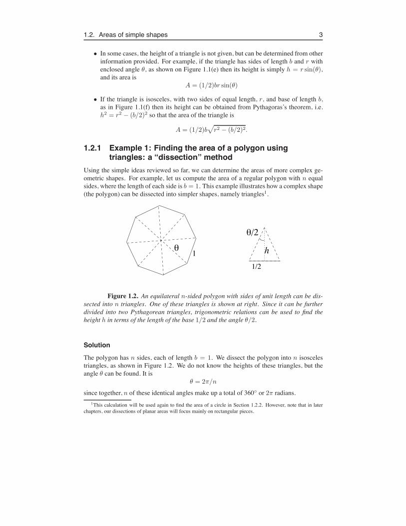
1.2.1 Example 1: Finding the area of a polygon usingtriangles: a “dissection” method

Using the simple ideas reviewed so far, we can determine the areas of more complex ge-ometric shapes. For example, let us compute the area of a regular polygon with n equalsides, where the length of each side is b = 1. This example illustrates how a complex shape(the polygon) can be dissected into simpler shapes, namely triangles1.

hθ 11/2

θ/2

Figure 1.2. An equilateral n-sided polygon with sides of unit length can be dis-sected into n triangles. One of these triangles is shown at right. Since it can be furtherdivided into two Pythagorean triangles, trigonometric relations can be used to find theheight h in terms of the length of the base 1/2 and the angle !/2.

Solution

The polygon has n sides, each of length b = 1. We dissect the polygon into n isoscelestriangles, as shown in Figure 1.2. We do not know the heights of these triangles, but theangle ! can be found. It is

! = 2"/n

since together, n of these identical angles make up a total of 360! or 2" radians.1This calculation will be used again to find the area of a circle in Section 1.2.2. However, note that in later

chapters, our dissections of planar areas will focus mainly on rectangular pieces.


Let h stand for the height of one of the triangles in the dissected polygon. Thentrigonometric relations relate the height to the base length as follows:

oppadj

=b/2

h= tan(!/2)

Using the fact that ! = 2"/n, and rearranging the above expression, we get

h =b

2 tan("/n)

Thus, the area of each of the n triangles is

A =1

2bh =

1

2b

"b

2 tan("/n)

#

.

The statement of the problem specifies that b = 1, so

A =1

2

"1

2 tan("/n)

#

.

The area of the entire polygon is then n times this, namely

An-gon =n

4 tan("/n).

For example, the area of a square (a polygon with 4 equal sides, n = 4) is

Asquare =4

4 tan("/4)=

1

tan("/4)= 1,

where we have used the fact that tan("/4) = 1.As a second example, the area of a hexagon (6 sided polygon, i.e. n = 6) is

Ahexagon =6

4 tan("/6)=

3

2(1/"

3)=

3"

3

2.

Here we used the fact that tan("/6) = 1/"

3.

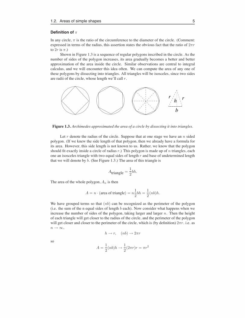
1.2.2 Example 2: How Archimedes discovered the area of acircle: dissect and “take a limit”

As we learn early in school the formula for the area of a circle of radius r, A = "r2.But how did this convenient formula come about? and how could we relate it to what weknow about simpler shapes whose areas we have discussed so far. Here we discuss howthis formula for the area of a circle was determined long ago by Archimedes using a clever“dissection” and approximation trick. We have already seen part of this idea in dissectinga polygon into triangles, in Section 1.2.1. Here we see a terrifically important second stepthat formed the “leap of faith” on which most of calculus is based, namely taking a limit asthe number of subdivisions increases 2.

First, we recall the definition of the constant ":2This idea has important parallels with our later development of integration. Here it involves adding up the

areas of triangles, and then taking a limit as the number of triangles gets larger. Later on, we do much the same,but using rectangles in the dissections.

1.2. Areas of simple shapes 5

Definition of "

In any circle, " is the ratio of the circumference to the diameter of the circle. (Comment:expressed in terms of the radius, this assertion states the obvious fact that the ratio of 2"rto 2r is ".)

Shown in Figure 1.3 is a sequence of regular polygons inscribed in the circle. As thenumber of sides of the polygon increases, its area gradually becomes a better and betterapproximation of the area inside the circle. Similar observations are central to integralcalculus, and we will encounter this idea often. We can compute the area of any one ofthese polygons by dissecting into triangles. All triangles will be isosceles, since two sidesare radii of the circle, whose length we’ll call r.

r r

b

h

Figure 1.3. Archimedes approximated the area of a circle by dissecting it into triangles.

Let r denote the radius of the circle. Suppose that at one stage we have an n sidedpolygon. (If we knew the side length of that polygon, then we already have a formula forits area. However, this side length is not known to us. Rather, we know that the polygonshould fit exactly inside a circle of radius r.) This polygon is made up of n triangles, eachone an isosceles triangle with two equal sides of length r and base of undetermined lengththat we will denote by b. (See Figure 1.3.) The area of this triangle is

Atriangle =1

2bh.

The area of the whole polygon, An is then

A = n · (area of triangle) = n1

2bh =

1

2(nb)h.

We have grouped terms so that (nb) can be recognized as the perimeter of the polygon(i.e. the sum of the n equal sides of length b each). Now consider what happens when weincrease the number of sides of the polygon, taking larger and larger n. Then the heightof each triangle will get closer to the radius of the circle, and the perimeter of the polygonwill get closer and closer to the perimeter of the circle, which is (by definition) 2"r. i.e. asn # $,

h # r, (nb) # 2"r

soA =

1

2(nb)h #

1

2(2"r)r = "r2


We have used the notation “#” to mean that in the limit, as n gets large, the quantity ofinterest “approaches” the value shown. This argument proves that the area of a circle mustbe

A = "r2.

One of the most important ideas contained in this little argument is that by approximating ashape by a larger and larger number of simple pieces (in this case, a large number of trian-gles), we get a better and better approximation of its area. This idea will appear again soon,but in most of our standard calculus computations, we will use a collection of rectangles,rather than triangles, to approximate areas of interesting regions in the plane.

Areas of other shapes

We concentrate here the area of a circle and of other shapes.

• The area of a circle of radius r is

A = "r2.

• The surface area of a sphere of radius r is

Sball = 4"r2.

• The surface area of a right circular cylinder of height h and base radius r is

Scyl = 2"rh.

Units

The units of area can be meters2 (m2), centimeters2 (cm2), square inches, etc.

1.3 Simple volumesLater in this course, we will also be computing the volumes of 3D shapes. As in the caseof areas, we collect below some basic formulae for volumes of elementary shapes. Thesewill be useful in our later discussions.

1. The volume of a cube of side length s (Figure 1.4a), is

V = s3.

2. The volume of a rectangular box of dimensions h, w, l (Figure 1.4b) is

V = hwl.

3. The volume of a cylinder of base area A and height h, as in Figure 1.4(c), is

V = Ah.

This applies for a cylinder with flat base of any shape, circular or not.

1.3. Simple volumes 7

r

(a) (b)

(c) (d)

sw

l

h

A

h

Figure 1.4. 3-dimensional shapes whose volumes are given by elementary formulae

4. In particular, the volume of a cylinder with a circular base of radius r, (e.g. a disk) is

V = h("r2).

5. The volume of a sphere of radius r (Figure 1.4d), is

V =4

3"r3.

6. The volume of a spherical shell (hollow sphere with a shell of some small thickness,# ) is approximately

V % # · (surface area of sphere) = 4"#r2.

7. Similarly, a cylindrical shell of radius r, height h and small thickness, # has volumegiven approximately by

V % # · (surface area of cylinder) = 2"#rh.

Units

The units of volume are meters3 (m3), centimeters3 (cm3), cubic inches, etc.


1.3.1 Example 3: The Tower of Hanoi: a tower of disksIn this example, we consider how elementary shapes discussed above can be used to de-termine volumes of more complex objects. The Tower of Hanoi is a shape consisting of anumber of stacked disks. It is a simple calculation to add up the volumes of these disks, butif the tower is large, and comprised of many disks, we would want some shortcut to avoidlong sums3.

Figure 1.5. Computing the volume of a set of disks. (This structure is sometimescalled the tower of Hanoi after a mathematical puzzle by the same name.)

(a) Compute the volume of a tower made up of four disks stacked up one on top ofthe other, as shown in Figure 1.5. Assume that the radii of the disks are 1, 2, 3, 4 units andthat each disk has height 1.

(b) Compute the volume of a tower made up of 100 such stacked disks, with radiir = 1, 2, . . . , 99, 100.

Solution

(a) The volume of the four-disk tower is calculated as follows:

V = V1 + V2 + V3 + V4,

where Vi is the volume of the i’th disk whose radius is r = i, i = 1, 2 . . . 4. The height ofeach disk is h = 1, so

V = ("12) + ("22) + ("32) + ("42) = "(1 + 4 + 9 + 16) = 30".

(b) The idea will be the same, but we have to calculate

V = "(12 + 22 + 32 + . . . + 992 + 1002).

It would be tedious to do this by adding up individual terms, and it is also cumbersometo write down the long list of terms that we will need to add up. This motivates inventingsome helpful notation, and finding some clever way of performing such calculations.

3Note that the idea of computing a volume of a radially symmetric 3D shape by dissection into disks will formone of the main themes in Chapter 5. Here, the sums of the volumes of disks is exactly the same as the volume ofthe tower. Later on, the disks will only approximate the true 3D volume, and a limit will be needed to arrive at a“true volume”.

1.4. Summations and the “Sigma” notation 9

1.4 Summations and the “Sigma” notationWe introduce the following notation for the operation of summing a list of numbers:

S = a1 + a2 + a3 + . . . + aN &N

$

k=1

ak.

The Greek symbol ! (“Sigma”) indicates summation. The symbol k used here iscalled the “index of summation” and it keeps track of where we are in the list of summands.The notation k = 1 that appears underneath ! indicates where the sum begins (i.e. whichterm starts off the series), and the superscript N tells us where it ends. We will be interestedin getting used to this notation, as well as in actually computing the value of the desiredsum using a variety of shortcuts.

Example 4a: Summation notation

Suppose we want to form the sum of ten numbers, each equal to 1. We would write this as

S = 1 + 1 + 1 + . . . 1 &10$

k=1

1.

The notation . . . signifies that we have left out some of the terms (out of laziness, or in caseswhere there are too many to conveniently write down.) We could have just as well writtenthe sum with another symbol (e.g. n) as the index, i.e. the same operation is implied by

10$

n=1

1.

To compute the value of the sum we use the elementary fact that the sum of ten ones is just10, so

S =10$

k=1

1 = 10.

Example 4b: Sum of squares

Expand and sum the following:

S =4

$

k=1

k2.

Solution

S =4

$

k=1

k2 = 1 + 22 + 32 + 42 = 1 + 4 + 9 + 16 = 30.

(We have already seen this sum in part (a) of The Tower of Hanoi.)


Example 4c: Common factors

Add up the following list of 100 numbers (only a few of them are shown):

S = 3 + 3 + 3 + 3 + . . . + 3.

Solution

There are 100 terms, all equal, so we can take out a common factor

S = 3 + 3 + 3 + 3 + . . . + 3 =100$

k=1

3 = 3100$

k=1

1 = 3(100) = 300.

Example 4d: Finding the pattern

Write the following terms in summation notation:

S =1

3+

1

9+

1

27+

1

81.

Solution

We recognize that there is a pattern in the sequence of terms, namely, each one is 1/3 raisedto an increasing integer power, i.e.

S =1

3+

"1

3

#2

+

"1

3

#3

+

"1

3

#4

.

We can represent this with the “Sigma” notation as follows:

S =4

$

n=1

"1

3

#n

.

The “index” n starts at 1, and counts up through 2, 3, and 4, while each term has the form of(1/3)n. This series is a geometric series, to be explored shortly. In most cases, a standardgeometric series starts off with the value 1. We can easily modify our notation to includeadditional terms, for example:

S =5

$

n=0

"1

3

#n

= 1 +1

3+

"1

3

#2

+

"1

3

#3

+

"1

3

#4

+

"1

3

#5

.

Learning how to compute the sum of such terms will be important to us, and will be de-scribed later on in this chapter.

1.4.1 Manipulations of sumsSince addition is commutative and distributive, sums of lists of numbers satisfy many con-venient properties. We give a few examples below:

1.5. Summation formulas 11

Example 5a: Simple operations

Simplify the following expression:

10$

k=1

2k !10$

k=3

2k.

Solution

10$

k=1

2k !10$

k=3

2k = (2 + 22 + 23 + · · · + 210) ! (23 + · · · + 210) = 2 + 22.

We could have arrived at this conclusion directly from

10$

k=1

2k !10$

k=3

2k =2$

k=1

2k = 2 + 22 = 2 + 4 = 6.

The idea is that all but the first two terms in the first sum will cancel. The only remainingterms are those corresponding to k = 1 and k = 2.

Example 5b: Expanding

Expand the following expression:

5$

n=0

(1 + 3n).

Solution

5$

n=0

(1 + 3n) =5

$

n=0

1 +5

$

n=0

3n.

1.5 Summation formulasIn this section we introduce a few examples of useful sums and give formulae that providea shortcut to dreary calculations.

The sum of consecutive integers (Gauss’ formula)

We first show that the sum of the first N integers is:

S = 1 + 2 + 3 + . . . + N =N

$

k=1

k =N(N + 1)

2. (1.1)


The following trick is due to Gauss. By aligning two copies of the above sum, onewritten backwards, we can easily add them up one by one vertically. We see that:

S = 1 + 2 + . . . + (N ! 1) + N+

S = N + (N ! 1) + . . . + 2 + 1

2S = (1 + N) + (1 + N) + . . . + (1 + N) + (1 + N)

Thus, there are N times the value (N + 1) above, so that

2S = N(1 + N), so S =N(1 + N)

2.

Thus, Gauss’ formula is confirmed.

Example: Adding up the first 1000 integers

Suppose we want to add up the first 1000 integers. This formula is very useful in whatwould otherwise be a huge calculation. We find that

S = 1 + 2 + 3 + . . . + 1000 =1000$

k=1

k =1000(1 + 1000)

2= 500(1001) = 500500.

Two other useful formulae are those for the sums of consecutive squares and ofconsecutive cubes:

The sum of the first N consecutive square integers

S2 = 12 + 22 + 32 + . . . + N2 =N

$

k=1

k2 =N(N + 1)(2N + 1)

6. (1.2)

The sum of the first N consecutive cube integers

S3 = 13 + 23 + 33 + . . . + N3 =N

$

k=1

k3 =

"N(N + 1)

2

#2

. (1.3)

In the Appendix, we show how the formula for the sum of square integers can beproved by a technique called mathematical induction.

1.5.1 Example 3, revisited: Volume of a Tower of HanoiArmed with the formula for the sum of squares, we can now return to the problem of com-puting the volume of a tower of 100 stacked disks of heights 1 and radii r = 1, 2, . . . , 99, 100.We have

V = "(12+22+32+. . .+992+1002) = "100$

k=1

k2 = "100(101)(201)

6= 338, 350" cubic units.

1.6. Summing the geometric series 13

Examples: Evaluating the sums

Compute the following two sums:

(a) Sa =20$

k=1

(2 ! 3k + 2k2), (b) Sb =50$

k=10

k.

Solutions

(a) We can separate this into three individual sums, each of which can be handled by alge-braic simplification and/or use of the summation formulae developed so far.

Sa =20$

k=1

(2 ! 3k + 2k2) = 220$

k=1

1 ! 320$

k=1

k + 220$

k=1

k2.

Thus, we get

Sa = 2(20)! 3

"20(21)

2

#

+ 2

"(20)(21)(41)

6

#

= 5150.

(b) We can express the second sum as a difference of two sums:

Sb =50$

k=10

k =

%50$

k=1

k

&

!

%9

$

k=1

k

&

.

ThusSb =

"50(51)

2!

9(10)

2

#

= 1275 ! 45 = 1230.

1.6 Summing the geometric seriesConsider a sum of terms that all have the form rk , where r is some real number and k isan integer power. We refer to a series of this type as a geometric series. We have alreadyseen one example of this type in a previous section. Below we will show that the sum ofsuch a series is given by:

SN = 1 + r + r2 + r3 + . . . + rN =N

$

k=0

rk =1 ! rN+1

1 ! r(1.4)

where r '= 1. We call this sum a (finite) geometric series. We would like to findan expression for terms of this form in the general case of any real number r, and finitenumber of terms N . First we note that there are N + 1 terms in this sum, so that if r = 1then

SN = 1 + 1 + 1 + . . . 1 = N + 1

(a total of N + 1 ones added.) If r '= 1 we have the following trick:

S = 1 + r + r2 + . . . + rN

!rS = r + r2 + . . . + rN+1


Subtracting leads to

S ! rS = (1 + r + r2 + . . . + rN ) ! (r + r2 + . . . + rN + rN+1)

Most of the terms on the right hand side cancel, leaving

S(1 ! r) = 1 ! rN+1.

Now dividing both sides by 1 ! r leads to

S =1 ! rN+1

1 ! r,

which was the formula to be established.

Example: Geometric series

Compute the following sum:

Sc =10$

k=0

2k.

Solution

This is a geometric series

Sc =10$

k=0

2k =1 ! 210+1

1 ! 2=

1 ! 2048

!1= 2047.

1.7 Prelude to infinite seriesSo far, we have looked at several examples of finite series, i.e. series in which there areonly a finite number of terms, N (where N is some integer). We would like to investigatehow the sum of a series behaves when more and more terms of the series are included. Itis evident that in many cases, such as Gauss’s series (1.1), or sums of squared or cubedintegers (e.g., Eqs. (1.2) and (1.3)), the series simply gets larger and larger as more termsare included. We say that such series diverge as N # $. Here we will look specificallyfor series that converge, i.e. have a finite sum, even as more and more terms are included4.

Let us focus again on the geometric series and determine its behaviour when thenumber of terms is increased. Our goal is to find a way of attaching a meaning to theexpression

Sn ="$

k=0

rk,

when the series becomes an infinite series. We will use the following definition:4Convergence and divergence of series is discussed in fuller depth in Chapter 10 in the context of Taylor Series.

However, these concepts are so important that it was felt necessary to introduce some preliminary ideas early inthe term.

1.7. Prelude to infinite series 15

1.7.1 The infinite geometric seriesDefinition

An infinite series that has a finite sum is said to be convergent. Otherwise it is divergent.

Definition

Suppose that S is an (infinite) series whose terms are ak. Then the partial sums, Sn, of thisseries are

Sn =n

$

k=0

ak.

We say that the sum of the infinite series is S, and write

S ="$

k=0

ak,

provided that

S = limn#"

n$

k=0

ak.

That is, we consider the infinite series as the limit of the partial sums as the number ofterms n is increased. In this case we also say that the infinite series converges to S.

We will see that only under certain circumstances will infinite series have a finitesum, and we will be interested in exploring two questions:

1. Under what circumstances does an infinite series have a finite sum.

2. What value does the partial sum approach as more and more terms are included.

In the case of a geometric series, the sum of the series, (1.4) depends on the numberof terms in the series, n via rn+1. Whenever r > 1, or r < !1, this term will get bigger inmagnitude as n increases, whereas, for 0 < r < 1, this term decreases in magnitude withn. We can say that

limn#"

rn+1 = 0 provided |r| < 1.

These observations are illustrated by two specific examples below. This leads to the fol-lowing conclusion:

The sum of an infinite geometric series,

S = 1 + r + r2 + . . . + rk + . . . ="$

k=0

rk,

exists provided |r| < 1 and isS =

1

1 ! r. (1.5)

Examples of convergent and divergent geometric series are discussed below.


1.7.2 Example: A geometric series that converges.Consider the geometric series with r = 1

2 , i.e.

Sn = 1 +1

2+

"1

2

#2

+

"1

2

#3

+ . . . +

"1

2

#n

=n

$

k=0

"1

2

#k

.

Then

Sn =1 ! (1/2)n+1

1 ! (1/2).

We observe that as n increases, i.e. as we retain more and more terms, we obtain

limn#"

Sn = limn#"

1 ! (1/2)n+1

1 ! (1/2)=

1

1 ! (1/2)= 2.

In this case, we write"$

n=0

"1

2

#n

= 1 +1

2+ (

1

2)2 + . . . = 2

and we say that “the (infinite) series converges to 2”.

1.7.3 Example: A geometric series that divergesIn contrast, we now investigate the case that r = 2: then the series consists of terms

Sn = 1 + 2 + 22 + 23 + . . . + 2n =n$

k=0

2k =1 ! 2n+1

1 ! 2= 2n+1 ! 1

We observe that as n grows larger, the sum continues to grow indefinitely. In this case, wesay that the sum does not converge, or, equivalently, that the sum diverges.

It is important to remember that an infinite series, i.e. a sum with infinitely manyterms added up, can exhibit either one of these two very different behaviours. It mayconverge in some cases, as the first example shows, or diverge (fail to converge) in othercases. We will see examples of each of these trends again. It is essential to be able todistinguish the two. Divergent series (or series that diverge under certain conditions) mustbe handled with particular care, for otherwise, we may find contradictions or seeminglyreasonable calculations that have meaningless results.

1.8 Application of geometric series to the branchingstructure of the lungs

In this section, we will compute the volume and surface area of the branched airways oflungs5. We use the summation formulae to arrive at the results, and we also illustrate howthe same calculation could be handled using a simple spreadsheet.

5This section provides an example of how to set up a biologically relevant calculation based on geometricseries. It is further studied in the homework problems. A similar example is given as an exercise for the studentin Lab 1 of this calculus course.

1.8. Application of geometric series to the branching structure of the lungs 17

Our lungs pack an amazingly large surface area into a confined volume. Most ofthe oxygen exchange takes place in tiny sacs called alveoli at the terminal branches of theairways passages. The bronchial tubes conduct air, and distribute it to the many smallerand smaller tubes that eventually lead to those alveoli. The principle of this efficient organfor oxygen exchange is that these very many small structures present a very large surfacearea. Oxygen from the air can diffuse across this area into the bloodstream very efficiently.

The lungs, and many other biological “distribution systems” are composed of abranched structure. The initial segment is quite large. It bifurcates into smaller segments,which then bifurcate further, and so on, resulting in a geometric expansion in the number ofbranches, their collective volume, length, etc. In this section, we apply geometric series toexplore this branched structure of the lung. We will construct a simple mathematical modeland explore its consequences. The model will consist in some well-formulated assumptionsabout the way that “daughter branches” are related to their “parent branch”. Based on theseassumptions, and on tools developed in this chapter, we will then predict properties of thestructure as a whole. We will be particularly interested in the volume V and the surfacearea S of the airway passages in the lungs6.

2

l0

r0

Segment 0

1

Figure 1.6. Air passages in the lungs consist of a branched structure. The indexn refers to the branch generation, starting from the initial segment, labeled 0. All segmentsare assumed to be cylindrical, with radius rn and length $n in the n’th generation.

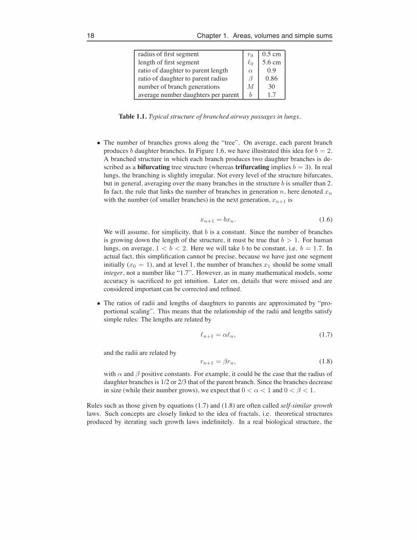
1.8.1 Assumptions• The airway passages consist of many “generations” of branched segments. We label

the largest segment with index “0”, and its daughter segments with index “1”, theirsuccessive daughters “2”, and so on down the structure from large to small branchsegments. We assume that there are M “generations”, i.e. the initial segment has un-dergone M subdivisions. Figure 1.6 shows only generations 0, 1, and 2. (Typically,for human lungs there can be up to 25-30 generations of branching.)

• At each generation, every segment is approximated as a cylinder of radius rn andlength $n.

6The surface area of the bronchial tubes does not actually absorb much oxygen, in humans. However, as anexample of summation, we will compute this area and compare how it grows to the growth of the volume fromone branching layer to the next.


radius of first segment r0 0.5 cmlength of first segment $0 5.6 cmratio of daughter to parent length % 0.9ratio of daughter to parent radius & 0.86number of branch generations M 30average number daughters per parent b 1.7

Table 1.1. Typical structure of branched airway passages in lungs.

• The number of branches grows along the “tree”. On average, each parent branchproduces b daughter branches. In Figure 1.6, we have illustrated this idea for b = 2.A branched structure in which each branch produces two daughter branches is de-scribed as a bifurcating tree structure (whereas trifurcating implies b = 3). In reallungs, the branching is slightly irregular. Not every level of the structure bifurcates,but in general, averaging over the many branches in the structure b is smaller than 2.In fact, the rule that links the number of branches in generation n, here denoted xn

with the number (of smaller branches) in the next generation, xn+1 is

xn+1 = bxn. (1.6)

We will assume, for simplicity, that b is a constant. Since the number of branchesis growing down the length of the structure, it must be true that b > 1. For humanlungs, on average, 1 < b < 2. Here we will take b to be constant, i.e. b = 1.7. Inactual fact, this simplification cannot be precise, because we have just one segmentinitially (x0 = 1), and at level 1, the number of branches x1 should be some smallinteger, not a number like “1.7”. However, as in many mathematical models, someaccuracy is sacrificed to get intuition. Later on, details that were missed and areconsidered important can be corrected and refined.

• The ratios of radii and lengths of daughters to parents are approximated by “pro-portional scaling”. This means that the relationship of the radii and lengths satisfysimple rules: The lengths are related by

$n+1 = %$n, (1.7)

and the radii are related byrn+1 = &rn, (1.8)

with % and & positive constants. For example, it could be the case that the radius ofdaughter branches is 1/2 or 2/3 that of the parent branch. Since the branches decreasein size (while their number grows), we expect that 0 < % < 1 and 0 < & < 1.

Rules such as those given by equations (1.7) and (1.8) are often called self-similar growthlaws. Such concepts are closely linked to the idea of fractals, i.e. theoretical structuresproduced by iterating such growth laws indefinitely. In a real biological structure, the


number of generations is finite. (However, in some cases, a finite geometric series is well-approximated by an infinite sum.)

Actual lungs are not fully symmetric branching structures, but the above approxi-mations are used here for simplicity. According to physiological measurements, the scalefactors for sizes of daughter to parent size are in the range 0.65 ( %, & ( 0.9. (K. G.Horsfield, G. Dart, D. E. Olson, and G. Cumming, (1971) J. Appl. Phys. 31, 207217.) Forthe purposes of this example, we will use the values of constants given in Table 1.1.

1.8.2 A simple geometric ruleThe three equations that govern the rules for successive branching, i.e. equations (1.6), (1.7),and (1.8), are examples of a very generic “geometric progression” recipe. Before returningto the problem at hand, let us examine the implications of this recursive rule, when it isapplied to generating the whole structure. Essentially, we will see that the rule linking twogenerations implies an exponential growth. To see this, let us write out a few first terms inthe progression of the sequence {xn}:

initial value: x0

first iteration: x1= bx0

second iteration: x2= bx1 = b(bx0) = b2x0

third iteration: x3= bx2 = b(b2x0) = b3x0

...

By the same pattern, at the n’th generation, the number of segments will be

n’th iteration: xn = bxn$1 = b(bxn$2) = b(b(bxn$3)) = . . . = (b · b · · · b)' () *

n factors

x0 = bnx0.

We have arrived at a simple, but important result, namely:

The rule linking two generations,xn = bxn$1 (1.9)

implies that the n’th generation will have grown by a factor bn, i.e.,

xn = bnx0. (1.10)

This connection between the rule linking two generations and the resulting number ofmembers at each generation is useful in other circumstances. Equation (1.9) is sometimescalled a recursion relation, and its solution is given by equation (1.10). We will use thesame idea to find the connection between the volumes, and surface areas of successivesegments in the branching structure.


1.8.3 Total number of segmentsWe used the result of Section 1.8.2 and the fact that there is one segment in the 0’th gener-ation, i.e. x0 = 1, to conclude that at the n’th generation, the number of segments is

xn = x0bn = 1 · bn = bn.

For example, if b = 2, the number of segments grows by powers of 2, so that the treebifurcates with the pattern 1, 2, 4, 8, etc.

To determine how many branch segments there are in total, we add up over all gen-erations, 0, 1, . . .M . This is a geometric series, whose sum we can compute. Using equa-tion (1.4), we find

N =M$

n=0

bn =

"1 ! bM+1

1 ! b

#

.

Given b and M , we can then predict the exact number of segments in the structure. Thecalculation is summarized further on for values of the branching parameter, b, and thenumber of branch generations, M , given in Table 1.1.

1.8.4 Total volume of airways in the lungSince each lung segment is assumed to be cylindrical, its volume is

vn = "r2n$n.

Here we mean just a single segment in the n’th generation of branches. (There are bn suchidentical segments in the n’th generation, and we will refer to the volume of all of themtogether as Vn below.)

The length and radius of segments also follow a geometric progression. In fact, thesame idea developed above can be used to relate the length and radius of a segment in then’th, generation segment to the length and radius of the original 0’th generation segment,namely,

$n = %$n$1 ) $n = %n$0,

andrn = &rn$1 ) rn = &nr0.

Thus the volume of one segment in generation n is

vn = "r2n$n = "(&nr0)

2(%n$0) = (%&2)n ("r20$0)

' () *

v0

.

This is just a product of the initial segment volume v0 = "r20$0, with the n’th power of a

certain factor(%, &). (That factor takes into account that both the radius and the length arebeing scaled down at every successive generation of branching.) Thus

vn = (%&2)nv0.


The total volume of all (bn) segments in the n’th layer is

Vn = bnvn = bn(%&2)nv0 = (b%&2

' () *

a

)n v0.

Here we have grouped terms together to reveal the simple structure of the relationship:one part of the expression is just the initial segment volume, while the other is now a“scale factor” that includes not only changes in length and radius, but also in the number ofbranches. Letting the constant a stand for that scale factor, a = (b%&2) leads to the resultthat the volume of all segments in the n’th layer is

Vn = anv0.

The total volume of the structure is obtained by summing the volumes obtained ateach layer. Since this is a geometric series, we can use the summation formula. i.e.,Equation (1.4). Accordingly, total airways volume is

V =30$

n=0

Vn = v0

30$

n=0

an = v0

"1 ! aM+1

1 ! a

#

.

The similarity of treatment with the previous calculation of number of branches is appar-ent. We compute the value of the constant a in Table 1.2, and find the total volume inSection 1.8.6.

1.8.5 Total surface area of the lung branchesThe surface area of a single segment at generation n, based on its cylindrical shape, is

sn = 2"rn$n = 2"(&nr0)(%n$0) = (%&)n (2"r0$0)

' () *

s0

,

where s0 is the surface area of the initial segment. Since there are bn branches at generationn, the total surface area of all the n’th generation branches is thus

Sn = bn(%&)ns0 = (b%&'()*

c

)ns0,

where we have let c stand for the scale factor c = (b%&). Thus,

Sn = cns0.

This reveals the similar nature of the problem. To find the total surface area of the airways,we sum up,

S = s0

M$

n=0

cn = s0

"1 ! cM+1

1 ! c

#

.

We compute the values of s0 and c in Table 1.2, and summarize final calculations of thetotal airways surface area in section 1.8.6.


volume of first segment v0 = "r20$0 4.4 cm3

surface area of first segment s0 = 2"r0$0 17.6 cm2

ratio of daughter to parent segment volume (%&2) 0.66564ratio of daughter to parent segment surface area (%&) 0.774ratio of net volumes in successive generations a = b%&2 1.131588ratio of net surface areas in successive generations c = b%& 1.3158

Table 1.2. Volume, surface area, scale factors, and other derived quantities. Be-cause a and c are bases that will be raised to large powers, it is important to that theirvalues are fairly accurate, so we keep more significant figures.

1.8.6 Summary of predictions for specific parameter valuesBy setting up the model in the above way, we have revealed that each quantity in the struc-ture obeys a simple geometric series, but with distinct “bases” b, a and c and coefficients1, v0, and s0. This approach has shown that the formula for geometric series applies ineach case. Now it remains to merely “plug in” the appropriate quantities. In this section,we collect our results, use the sample values for a model “human lung” given in Table 1.1,or the resulting derived scale factors and quantities in Table 1.2 to finish the task at hand.

Total number of segments

N =M$

n=0

bn =

"1 ! bM+1

1 ! b

#

=

"1 ! (1.7)31

1 ! 1.7

#

= 1.9898 · 107 % 2 · 107.

According to this calculation, there are a total of about 20 million branch segments overall(including all layers, form top to bottom) in the entire structure!

Total volume of airways

Using the values for a and v0 computed in Table 1.2, we find that the total volume of allsegments in the n’th generation is

V = v0

30$

n=0

an = v0

"1 ! aM+1

1 ! a

#

= 4.4(1 ! 1.13158831)

(1 ! 1.131588)= 1510.3 cm3.

Recall that 1 litre = 1000 cm3. Then we have found that the lung airways contain about 1.5litres.


Total surface area of airways

Using the values of s0 and c in Table 1.2, the total surface area of the tubes that make upthe airways is

S = s0

M$

n=0

cn = s0

"1 ! cM+1

1 ! c

#

= 17.6(1 ! 1.315831)

(1 ! 1.3158)= 2.76 · 105 cm2.

There are 100 cm per meter, and (100)2 = 104 cm2 per m2. Thus, the area we havecomputed is equivalent to about 28 square meters!

1.8.7 Exploring the problem numericallyUp to now, all calculations were done using the formulae developed for geometric series.However, sometimes it is more convenient to devise a computer algorithm to implement“rules” and perform repetitive calculations in a problem such as discussed here. The ad-vantage of that approach is that it eliminates tedious calculations by hand, and, in caseswhere summation formulae are not know to us, reduces the need for analytical computa-tions. It can also provide a shortcut to visual summary of the results. The disadvantage isthat it can be less obvious how each of the values of parameters assigned to the problemaffects the final answers.

A spreadsheet is an ideal tool for exploring iterated rules such as those given in thelung branching problem7. In Figure 1.7 we show the volumes and surface areas associatedwith the lung airways for parameter values discussed above. Both layer by layer values andcumulative sums leading to total volume and surface area are shown in each of (a) and (c).In (b) and (d), we compare these results to similar graphs in the case that one parameter, thebranching number, b is adjusted from 1.7 (original value) to 2. The contrast between thegraphs shows how such a small change in this parameter can significantly affect the results.

1.8.8 For further independent studyThe following problems can be used for further independent exploration of these ideas.

1. In our model, we have assumed that, on average, a parent branch has only “1.7”daughter branches, i.e. that b = 1.7. Suppose we had assumed that b = 2. Whatwould the total volume V be in that case, keeping all other parameters the same?Explain why this is biologically impossible in the case M = 30 generations. Forwhat value of M would b = 2 lead to a reasonable result?

2. Suppose that the first 5 generations of branching produce 2 daughters each, but thenfrom generation 6 on, the branching number is b = 1.7. How would you set up thisvariant of the model? How would this affect the calculated volume?

3. In the problem we explored, the net volume and surface area keep growing by largerand larger increments at each “generation” of branching. We would describe this as“unbounded growth”. Explain why this is the case, paying particular attention to thescale factors a and c.

7See Lab 1 for a similar problem that is also investigated using a spreadsheet.


Cumulative volume to layer n

Vn = Volume of layer n||V

-0.5 30.50.0

1500.0Cumulative volume to layer n

Vn = Volume of layer n

-0.5 30.50.0

1500.0

(a) (b)

Cumulative surface area to n’th layer

surface area of n’th layer

-0.5 30.50.0

250000.0Cumulative surface area to n’th layer

surface area of n’th layer-0.5 30.5

0.0

250000.0

(c) (d)

Figure 1.7. (a) Vn, the volume of layer n (red bars), and the cumulative volumedown to layer n (yellow bars) are shown for parameters given in Table 1.1. (b) Same as (a)but assuming that parent segments always produce two daughter branches (i.e. b = 2). Thegraphs in (a) and (b) are shown on the same scale to accentuate the much more dramaticgrowth in (b). (c) and (d): same idea showing the surface area of n’th layer (green) andthe cumulative surface area to layer n (blue) for original parameters (in c), as well as forthe value b = 2 (in d).

4. Suppose we want a set of tubes with a large surface area but small total volume.Which single factor or parameter should we change (and how should we change it) tocorrect this feature of the model, i.e. to predict that the total volume of the branchingtubes remains roughly constant while the surface area increases as branching layersare added.

5. Determine how the branching properties of real human lungs differs from our as-sumed model, and use similar ideas to refine and correct our estimates. You maywant to investigate what is known about the actual branching parameter b, the num-ber of generations of branches, M , and the ratios of lengths and radii that we haveassumed. Alternately, you may wish to find parameters for other species and do a

1.9. Summary 25

comparative study of lungs in a variety of animal sizes.

6. Branching structures are ubiquitous in biology. Many species of plants are basedon a regular geometric sequence of branching. Consider a tree that trifurcates (i.e.produces 3 new daughter branches per parent branch, b = 3). Explain (a) Whatbiological problem is to be solved in creating such a structure (b) What sorts ofconstraints must be satisfied by the branching parameters to lead to a viable structure.This is an open-ended problem.

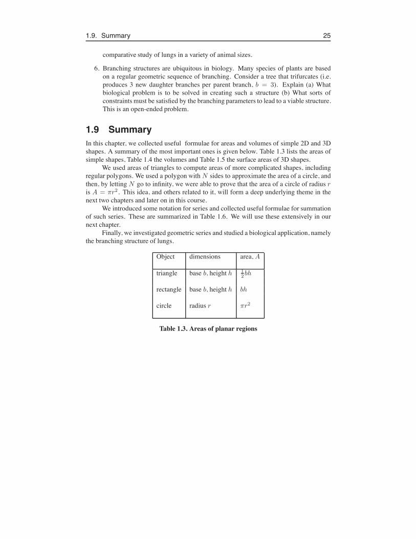
1.9 SummaryIn this chapter, we collected useful formulae for areas and volumes of simple 2D and 3Dshapes. A summary of the most important ones is given below. Table 1.3 lists the areas ofsimple shapes, Table 1.4 the volumes and Table 1.5 the surface areas of 3D shapes.

We used areas of triangles to compute areas of more complicated shapes, includingregular polygons. We used a polygon with N sides to approximate the area of a circle, andthen, by letting N go to infinity, we were able to prove that the area of a circle of radius ris A = "r2. This idea, and others related to it, will form a deep underlying theme in thenext two chapters and later on in this course.

We introduced some notation for series and collected useful formulae for summationof such series. These are summarized in Table 1.6. We will use these extensively in ournext chapter.

Finally, we investigated geometric series and studied a biological application, namelythe branching structure of lungs.

Object dimensions area, A

triangle base b, height h 12bh

rectangle base b, height h bh

circle radius r "r2

Table 1.3. Areas of planar regions


Object dimensions volume, V

box base b, height h, width w hwb

circular cylinder radius r, height h "r2h

sphere radius r 43"r3

cylindrical shell* radius r, height h, thickness # 2"rh#

spherical shell* radius r, thickness # 4"r2#

Table 1.4. Volumes of 3D shapes. * Assumes a thin shell, i.e. small # .

Object dimensions surface area, S

box base b, height h, width w 2(bh + bw + hw)

circular cylinder radius r, height h 2"rh

sphere radius r 4"r2

Table 1.5. Surface areas of 3D shapes

Sum Notation Formula Comment

1 + 2 + 3 + . . . + N+N

k=1 k N(1+N)2 Gauss’ formula

12 + 22 + 32 + . . . + N2+N

k=1 k2 N(N+1)(2N+1)6 Sum of squares

13 + 23 + 33 + . . . + N3+N

k=1 k3,

N(N+1)2

-2Sum of cubes

1 + r + r2 + r3 . . . rN+N

k=0 rk 1$rN+1

1$r Geometric sum

Table 1.6. Useful summation formulae.

areas, volumes and simple sums - undergrad...

Documents