Arithmetic and topology of hypertoric varieties

Nicholas Proudfoot1

Department of Mathematics, University of Texas, Austin, TX 78712

Benjamin Webster2

Department of Mathematics, University of California, Berkeley, CA 94720

Abstract. A hypertoric variety is a quaternionic analogue of a toric variety. Just asthe topology of toric varieties is closely related to the combinatorics of polytopes, thetopology of hypertoric varieties interacts richly with the combinatorics of hyperplanearrangements and matroids. Using finite field methods, we obtain combinatorial de-scriptions of the Betti numbers of hypertoric varieties, both for ordinary cohomologyin the smooth case and intersection cohomology in the singular case. We also introducea conjectural ring structure on the intersection cohomology of a hypertoric variety.

Let T k be an algebraic torus acting linearly and effectively on an affine space An, by which

we mean a vector space over an unspecified field, or even over the integers. Though much

of our paper is devoted to the finite field case, for the purposes of the introduction one may

simply think of a complex vector space. A character α of T k defines a lift of the action to the

trivial line bundle on An, and the corresponding geometric invariant theory (GIT) quotient

X = An//αT k is a toric variety.3 A hypertoric variety is a symplectic quotient

M = T ∗An////(α,0)Tk = µ−1(0)//αT

k, (1)

where µ : T ∗An → (tk)∗ is the algebraic moment map for the T k action on T ∗An. Over the

complex numbers, this construction may be interpreted as a hyperkahler quotient [BD, §3],

or equivalently as a real symplectic quotient of µ−1(0) by the compact form of T k. For this

reason, M may be thought of as a ‘quaternionic’ or hyperkahler analogue of X. In this

paper, however, we will focus on the algebro-geometric construction, which lets us work over

arbitrary fields.

The data of T k acting on An, along with the character α, can be conveniently encoded

by an arrangement A of cooriented hyperplanes in an affine space of dimension d = n − k.

The topology of the corresponding complex toric variety X(A)C is deeply related to the

combinatorics of the polytope cut out by A over the real numbers [S1, S2]. The hypertoric

variety M(A) is sensitive to a different side of the combinatorial data. As a topological

space, the complex variety M(A)C does not depend on the coorientations of the hyperplanes

[HP, 2.2], and hence has little relationship to the polytope that controls X(A). Instead, the

1Supported by the Clay Mathematics Institute Liftoff Program and the National Science FoundationPostdoctoral Research Fellowship.

2Supported by the National Science Foundation Graduate Research Fellowship.3See [P2] for an elementary definition of GIT quotients, and an exposition of toric varieties from this

perspective. The reader with a more differential bent can think of X as a real symplectic quotient of Cn bythe compact torus sitting inside of T k. This is not to be confused with the algebraic (or complex) symplecticquotient of Equation (1).

1

topology of M(A)C interacts richly with the combinatorics of the matroid associated to A,

as explained in [Ha]. We now describe the sort of combinatorial structures that arise in this

setting.

Let ∆ be a simplicial complex of dimension d− 1 on the ground set {1, . . . , n}. The f-

vector of ∆ is the (d+1)-tuple (f0, . . . , fd), where fi is the number of faces of ∆ of cardinality

i (and therefore of dimension i − 1). The h-vector (h0, . . . , hd) and h-polynomial h∆(q)

of ∆ are defined by the equations

h∆(q) =d∑i=0

hi qi =

d∑i=0

fi qi(1− q)d−i.

To each simplicial complex ∆, we associate its Stanley-Reisner ring SR(∆), which is

defined to be the the quotient of C[e1, . . . , en] by the ideal generated by the monomials∏i∈S ei for all non-faces S of ∆. The complex ∆ is called Cohen-Macaulay if there exists

a d-dimensional subspace L ⊆ SR(∆)1 such that SR(∆) is a free module over the polynomial

ring SymL. Such a subspace is called a linear system of parameters. If ∆ is Cohen-

Macaulay and L is a linear system of parameters for ∆, then SR0(∆) := SR(∆) ⊗SymL Chas Hilbert series equal to h∆(q) [S3, 5.9].

Let A = {H1, . . . , Hn} be a collection of labeled hyperplanes in a vector space V , and let

ai ∈ V ∗ be a nonzero normal vector to Hi for all i. The matroid complex ∆A associated

to A is the collection of sets S ⊆ {1, . . . , n} such that {ai | i ∈ S} is linearly independent.

A circuit of ∆A is a minimal dependent set. Let σ be an ordering of the set {1, . . . , n}.A σ-broken circuit of ∆A is a set C r {i}, where C is a circuit, and i is the σ-minimal

element of C. The σ-broken circuit complex bcσ∆A is defined to be the collection of

subsets of {1, . . . , n} that do not contain a σ-broken circuit. The two complexes ∆A and

bcσ∆A are both Cohen-Macaulay (in fact shellable [Bj, §7.3 & §7.4]); their h-polynomials

will be denoted hA(q) and hbrA (q), respectively. As the notation suggests, the polynomial

hbrA (q) is independent of our choice of ordering σ [Bj, §7.4].

Let A be a central hyperplane arrangement, and A a simplification of A. By this we mean

that all of the hyperplanes in A pass through the origin, and A is obtained by translating

those hyperplanes away from the origin in such a way so that all nonempty intersections are

generic. Then M(A) is an affine cone, and M(A) is an orbifold resolution of M(A). Our

goal is to study the topology of the complex varieties M(A)C and M(A)C, relating them

to the combinatorics of the arrangement A. To achieve this goal, we count points on the

corresponding varieties over finite fields.

Our approach to counting points on M(A) is motivated by a paper of Crawley-Boevey

and Van den Bergh [CBVdB], who work in the context of representations of quivers. In

Section 3 we use an exact sequence that appeared first in [CB] to obtain a combinatorial

formula for the number of Fq points of M(A). Then the Weil conjectures allow us to translate

this formula into a description of the Poincare polynomial of M(A)C (Theorem 3.5).

Theorem. The Poincare polynomial of M(A)C coincides with the h-polynomial of ∆A.

2

This theorem has been proven by different means in [BD, 6.7] and [HS, 1.2]. One notewor-

thy aspect of our approach is that it sheds light on a mysterious theorem of Buchstaber and

Panov [BP, §8], who produce a seemingly unrelated space with the same Poincare polynomial

(see Remark 3.6).

In the case of the singular variety M(A), we follow the example of Kazhdan and Lusztig

[KL, §4], who study the singularities of Schubert varieties. These singularities are measured

by local intersection cohomology Poincare polynomials, and Kazhdan and Lusztig obtain a

recursive formula for these polynomials using Deligne’s extension of the Weil conjectures. In

our paper, we extend the argument in [KL, 4.2] to apply to more general classes of varieties.

Roughly speaking, we consider a collection of stratified affine cones with polynomial point

count, which is closed under taking closures of strata, and normal cones to strata. (For

details, see Theorem 4.1.) In Section 2 we give such a stratification of M(A), and in Section

4 we obtain the following new result (Theorem 4.3).

Theorem. The intersection cohomology Poincare polynomial of M(A)C coincides with the

h-polynomial of bcσ∆A.

Section 5 is devoted to the comparison of the two h-polynomials using the decomposition

theorem of [BBD, 6.2.5]. The map from M(A) to M(A) is semismall (Corollary 2.7), hence

the decomposition theorem expresses the cohomology of M(A)C in terms of the intersection

cohomology of the strata of M(A)C and the cohomology of the fibers of the resolution

(Equation (13)). By our previous results, we thus obtain a combinatorial formula relating

the h-numbers of a matroid complex to those of its broken circuit complex. This formula

turns out to be a special case of the Kook-Reiner-Stanton convolution formula, which is

proven from a strictly combinatorial perspective in [KRS, 1].

We note that this suggests yet another avenue leading to the computation of the Betti

numbers of M(A)C. Knowing only the intersection Betti numbers of M(A)C, we could have

computed these numbers using the KRS formula and the recursion that we obtained from the

decomposition theorem. This approach is one that generalizes naturally to other settings.

For example, Nakajima’s quiver varieties form a class of stratified affine varieties which is

closed under taking closures of strata and normal cones to strata [Na, §3]. These varieties

have semismall resolutions whose Betti numbers are relevant to the representation theory of

Kac-Moody algebras, and are the subject of an outstanding conjecture of Lusztig [Lu, 8]. If a

polynomial point count for the singular varieties could be obtained, then the decomposition

theorem would provide recursive formulas for the Betti numbers of the smooth ones.

Section 6 deals with the problem of ring structures. Hausel and Sturmfels show that

the cohomology ring of M(A)C is isomorphic to SR0(∆A), which strengthens Theorem 3.5.

Intersection cohomology is in general only a group, so we have no analogous theorem to

prove for M(A)C. When A is a unimodular arrangement, however, we define a ring R0(A)

which is isomorphic to the intersection cohomology of M(A)C as a graded vector space. This

ring does not depend on a choice of ordering σ of the set {1, . . . , n}, but it degenerates flatly

to SR0(bcσ∆A) for any σ (Theorem 6.2). We conjecture that this isomorphism is natural,

3

and that the multiplicative structure can be interpreted in terms of the geometry of M(A)C(Conjecture 6.4).

Acknowledgments. The authors are grateful to Tom Braden, Mark Haiman, Joel Kam-

nitzer, Brian Osserman, Vic Reiner, David Speyer, and Ed Swartz for invaluable discussions.

1 Hypertoric varieties

Let T n and T d be split algebraic tori defined over Z, with Lie algebras tn and td. Let

{x1, . . . , xn} be a basis for tn = Lie(T n), and let {e1, . . . , en} be the dual basis for the dual

lattice (tn)∗. Suppose given n nonzero integer vectors {a1, . . . , an} ⊆ td such that the map

tn → td taking xi to ai has rank d, and let tk be the kernel of this map. Then we have an

exact sequence

0 −→ tkι−→ tn −→ td −→ 0, (2)

which exponentiates to an exact sequence of groups

0 −→ T k −→ T n −→ T d −→ 0, (3)

where T k = ker(T n → T d

). Thus T k is an algebraic group with Lie algebra tk, which is

connected if and only if the vectors {ai} span the lattice td over the integers. Every algebraic

subgroup of T n arises in this way.

Consider the cotangent bundle T ∗An ∼= An × (An)∗ along with its natural algebraic sym-

plectic form

ω =∑

dzi ∧ dwi,

where z and w are coordinates on An and (An)∗, respectively. The restriction to T k of the

standard action of T n on T ∗An is hamiltonian, with moment map

µ(z, w) = ι∗n∑i=1

(ziwi) ei.

Suppose given an integral element α ∈ (tk)∗. This descends via the exponential map to a

character of T k, which defines a lift of the action of T k to the trivial bundle on T ∗An. The

symplectic quotient

M = T ∗An////αTk = µ−1(0)//αT

k

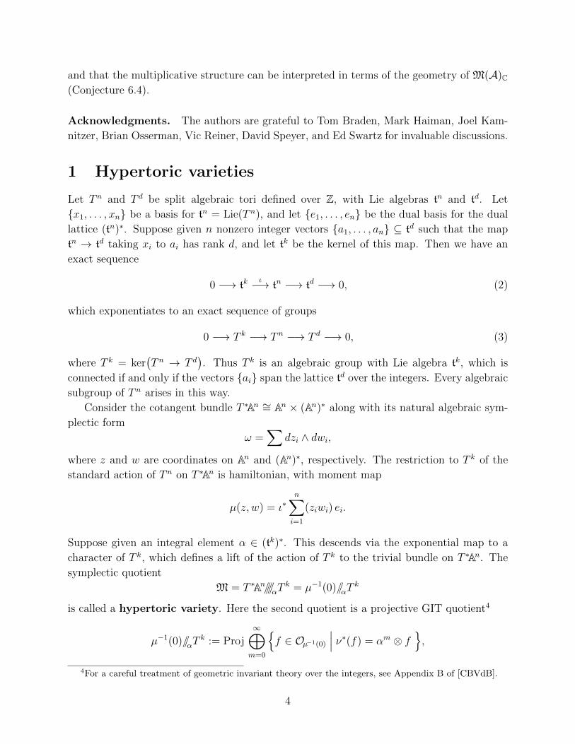
is called a hypertoric variety. Here the second quotient is a projective GIT quotient4

µ−1(0)//αTk := Proj

∞⊕m=0

{f ∈ Oµ−1(0)

∣∣∣ ν∗(f) = αm ⊗ f},

4For a careful treatment of geometric invariant theory over the integers, see Appendix B of [CBVdB].

4

where

ν∗ : Oµ−1(0) → OTk×µ−1(0)∼= OTk ⊗Oµ−1(0)

is the map on functions induced by the action map ν : T k×µ−1(0)→ µ−1(0). If α is omitted

from the subscript, it will be understood to be equal to zero. The hypertoric variety M is a

symplectic variety of dimension 2d, and admits an effective hyperhamiltonian action of the

torus T d = T n/T k, with moment map

Φ[z, w] =n∑i=1

(ziwi) ei ∈ ker(ι∗) = (td)∗.

Here [z, w] is used to denote the image in M of a pair (z, w) with closed T k-orbit in µ−1(0).

Remark 1.1. The word ‘hypertoric’ comes from the fact that the complex variety MC may

be constructed as a hyperkahler quotient of T ∗Cn by the compact real form of T k, thus making

it a ‘hyperkahler analogue’ of the toric variety X = Cn//αTk. This was the original approach

of Bielawski and Dancer [BD], who used the name ‘toric hyperkahler manifolds’. For more

on the general theory of hyperkahler analogues of Kahler quotients, see [P1].

It is convenient to encode the data that were used to construct M in terms of an ar-

rangement of affine hyperplanes in (td)∗, with some additional structure. A weighted,

cooriented, affine hyperplane H ⊆ (td)∗ is a hyperplane along with a choice of nonzero

integer normal vector a ∈ td. Here “affine” means that H need not pass through the origin,

and “weighted” means that a is not required to be primitive. Let r = (r1, . . . , rn) ∈ (tn)∗ be

a lift of α along ι∗, and let

Hi = {v ∈ (td)∗ | v · ai + ri = 0}

be the weighted, cooriented, affine hyperplane with normal vector ai ∈ td. We will denote the

arrangement {H1, . . . , Hn} by A, and the associated hypertoric variety by M(A). Choosing

a different lift r′ of α corresponds geometrically to translating A inside of (td)∗. The rank of

the lattice spanned by the vectors {ai} is called the rank of A; in our case, we have already

made the assumption that A has rank d. Observe that A is defined over the integers,

and therefore may be realized over any field. Intuitively, it is useful to think of A as an

arrangement of real hyperplanes, but in Section 4 we will need to consider the complement

of A over a finite field.

Remark 1.2. We note that we allow repetitions of hyperplanes in our arrangement (A may

be a multi-set), and that a repeated occurrence of a particular hyperplane is not the same

as a single occurrence of that hyperplane with weight 2. On the other hand, little is lost by

restricting one’s attention to arrangements of distinct hyperplanes of weight one.

We call the arrangement A simple if every subset of m hyperplanes with nonempty

intersection intersects in codimension m. We call A unimodular if every collection of d

linearly independent vectors {ai1 , . . . , aid} spans td over the integers. An arrangement which

is both simple and unimodular is called smooth.

5

Theorem 1.3. [BD, 3.2 & 3.3] The hypertoric variety M(A) has at worst orbifold (finite

quotient) singularities if and only if A is simple, and is smooth if and only if A is smooth.

Let A = {H1, . . . , Hn} be a central arrangement, meaning that ri = 0 for all i. Let

A = {H1, . . . , Hn} be a simplification of A, by which we mean an arrangement defined by

the same vectors {ai} ⊂ td, but with a different choice of r ∈ (tn)∗, such that A is simple.

This corresponds to translating each of the hyperplanes in A away from the origin by some

generic amount. We then have

M(A) = Proj∞⊕m=0

OTkµ−1(0) = SpecOTkµ−1(0) = SpecOM(A),

hence there is a surjective, projective map π : M(A) → M(A). Geometrically, π may be

understood to be the map induced by the T k-equivariant inclusion of µ−1(0)α−st into µ−1(0),

where µ−1(0)α−st is the stable locus for the linearization of the T k action given by α = ι∗(r).

The central fiber L(A) = π−1(0) is called the core of M(A).

Theorem 1.4. [BD, §6],[HS, 6.4] The core L(A) is isomorphic to a union of toric varieties

with moment polytopes given by the bounded complex of A. Over the complex numbers,

L(A)C is a T dR-equivariant deformation retract of M(A)C, where T dR∼= U(1)d is the compact

real form of T dC.

It follows that the dimension of the core is at most d, with equality if and only A is

coloop-free (see Remark 2.3).

Example 1.5. The two arrangements pictured below are each simplifications of a central

arrangement of four hyperplanes in R2, in which the second and third hyperplane coincide.

All hyperplanes are taken with weight 1, and coorientations may be chosen arbitrarily.

4

1

3

1

2

2

3

4

Consider the complex hypertoric varieties associated to these two arrangements. Both are

obtained as symplectic quotients of T ∗C4 by the same T 2 action, but with different choices

of character. Both varieties are resolutions of the affine variety given by the associated

central arrangement. The hypertoric variety associated to the left-hand arrangement has a

core consisting of a projective plane glued to a Hirzebruch surface along a projective line.

The hypertoric variety associated to the right-hand arrangement has a core consisting of two

projective planes glued together at a point. As manifolds, they are diffeomorphic, as are any

two complex hypertoric varieties corresponding to different simplifications of the same central

arrangement [HP, 2.1].

6

2 The stratification

Let A be a rank d central arrangement of n weighted, cooriented hyperplanes in (td)∗. Our

goal for this section is to define and analyze a stratification of the singular affine variety

M(A). This stratification will be a refinement of the Sjamaar-Lerman stratification, intro-

duced for real symplectic quotients in [SL], and adapted to the algebraic setting in [Na, §3].

Our refinement will prove to be more natural from a combinatorial perspective (see Remark

2.3).

Given any subset S ⊆ {1, . . . , n}, let HS = ∩i∈SHi. A flat of A is a subset F ⊆ {1, . . . , n}such that F = {i | Hi ⊇ HF}. We let L(A) denote the lattice of flats for the arrangement

A. For any flat F , we define the restriction

AF := {Hi ∩HF | i /∈ F},

an arrangement of |F c| hyperplanes in the affine space HF , and the localization

AF := {Hi/HF | i ∈ F},

an arrangement of |F | hyperplanes in the affine space (td)∗/HF . The lattice L(AF ) is iso-

morphic to the sublattice of L(A) consisting of those flats which contain F ; likewise, L(AF )

may be identified with the sublattice of L(A) consisting of flats contained in F . We define

the rank of a flat rkF = rkAF , and the corank crkF = rkAF = rkA − rkF . Given a

simplification A of A, there is a natural simplification AF of the localization.

We now fix notation regarding the various tori associated to the localization and restric-

tion of A at F . The AF analogue of the exact sequence (2) is

0→ t→ tF → trkF → 0,

where tF is the coordinate subtorus of tn supported on F , trkF ∼= HF is the image of tF in

td, and t = tk ∩ tF . Similarly, the restriction AF corresponds to an exact sequence

0→ t→ tFc → tcrkF → 0,

where tFc

is the coordinate subtorus of tn supported on F c, tcrkF ∼= td/HF , and t = tk/t.

The tori T , T F , T rkF and T, T Fc, T crkF are defined analogously, as in the exact sequence (3).

Let T ∗AF and T ∗AF c be the cotangent bundles of the corresponding coordinate subspaces of

An. Then the hypertoric varieties M(AF ) and M(AF ) are obtained as symplectic quotients

of T ∗AF and T ∗AF c by T and T , respectively.

Proposition 2.1. Let F be a flat of A. The subvariety of M(A) given by the equations

zi = wi = 0 for all i ∈ F is isomorphic to M(AF ).

Proof: The inclusion of T ∗AF c into T ∗An is T k-equivariant, where the action of T k on T ∗AF c

factors through T . The Lie coalgebra t∗ of T includes into (tk)∗, and the T k-moment map

7

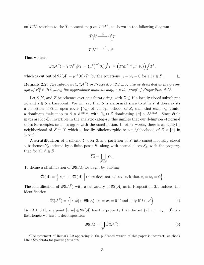
on T ∗An restricts to the T -moment map on T ∗AF c , as shown in the following diagram.

T ∗An µ // (tk)∗

T ∗AF c µF //

OO

t∗

OO

Thus we have

M(AF ) = T ∗AF c////T =(µF)−1

(0)//T ∼=

(T ∗AF c ∩ µ−1(0)

)//T k,

which is cut out of M(A) = µ−1(0)/T k by the equations zi = wi = 0 for all i ∈ F .

Remark 2.2. The subvariety M(AF ) in Proposition 2.1 may also be described as the preim-

age of HRF ⊕HC

F along the hyperkahler moment map; see the proof of Proposition 5.1.5

Let S, Y , and Z be schemes over an arbitary ring, with Z ⊆ Y a locally closed subscheme

Z, and s ∈ S a basepoint. We will say that S is a normal slice to Z in Y if there exists

a collection of etale open cover {Uα} of a neighborhood of Z, such that each Uα admits

a dominant etale map to S × AdimZ , with Uα ∩ Z dominating {s} × AdimZ . Since etale

maps are locally invertible in the analytic category, this implies that our definition of normal

slices for complex schemes agree with the usual notion. In other words, there is an analytic

neighborhood of Z in Y which is locally biholomorphic to a neighborhood of Z × {s} in

Z × S.

A stratification of a scheme Y over Z is a partition of Y into smooth, locally closed

subschemes Yβ indexed by a finite poset B, along with normal slices Sβ, with the property

that for all β ∈ B,

Yβ =⊔β′≤β

Yβ′ .

To define a stratification of M(A), we begin by putting

M(A) ={

[z, w] ∈M(A)∣∣∣ there does not exist i such that zi = wi = 0

}.

The identification of M(AF ) with a subvariety of M(A) as in Proposition 2.1 induces the

identification

M(AF ) ={

[z, w] ∈M(A)∣∣∣ zi = wi = 0 if and only if i ∈ F

}. (4)

By [BD, 3.1], any point [z, w] ∈ M(A) has the property that the set {i | zi = wi = 0} is a

flat, hence we have a decomposition

M(A) =⊔F

M(AF ). (5)

5The statement of Remark 2.2 appearing in the published version of this paper is incorrect; we thankLinus Setiabrata for pointing this out.

8

One interpretation of our decomposition is that points are grouped according to the stabi-

lizers in T n of their lifts to µ−1(0). This is therefore a refinement of the Sjamaar-Lerman

stratification [SL, §2], which groups points by their stabilizers in the subtorus T k. It fol-

lows from the defining property of a moment map that M(A) is smooth, and therefore that

each piece of the decomposition is smooth. To see that our decomposition is a stratification

we must produce normal slices to the strata, which we will do in Lemma 2.4. The largest

stratum M(A) will be referred to as the generic stratum of M(A).

Remark 2.3. If [z, w] ∈ M(AF ), then the stabilizer of (z, w) ∈ µ−1(0) is equal to T =

T k ∩ T F . An element i ∈ F is called a coloop of F if ai may not be expressed as a linear

combination of {aj | j ∈ F r {i}}. If F and G are two flats, then T k ∩ T F = T k ∩ TG if and

only if F and G agree after deleting all coloops. Hence the Sjamaar-Lerman stratification of

M(A) is naturally indexed by coloop-free flats, rather than all flats.

Lemma 2.4. The variety M(AF ) is a normal slice to M(AF ) ⊆M(A), thus the decompo-

sition of Equation (5) is a stratification.

Proof: Let S be a subset of F c such that the coordinate vectors in (tFc)∗ indexed by S

descend to a basis of t∗, and let

WS ={

[z, w] ∈M(A)∣∣∣ zi 6= 0 for all i ∈ S

}. (6)

Any element of WS may be represented by an element (z, w) ∈ µ−1(0) such that zi = 1 for

all i ∈ S, and any two such representations differ by a element of the subtorus T ⊆ T k. Next

observe that the coordinate projection of T ∗An onto T ∗AF takes µ−1(0) to the zero set of the

moment map for the action of T on T ∗AF . We may therefore define a map pF : WS →M(AF )

by taking an element of WS, representing it in the form described above, and projecting to

the F coordinates. This map is smooth on the locus M(AF ) ∩WS.

Suppose that y ∈ WS. By [BLR, 2.2.14], there is a neighborhood U of y in WS and a

smooth map η : U → AcrkF such that the restriction of pF to η−1(0) is etale. Let

ϑ = η × pF : U → AcrkF ×M(AF ).

Then the derivative of ϑ at y is a surjection, hence ϑ is smooth at y. Since its source and

target have the same dimension, it must be etale.

If y is not in S, then we may modify the definition of WS by changing some of the zito wi in Equation (6), and adjust the definition of the map pF accordingly. Then y will be

contained in the new set WS, and the proof will go through as before.

We next prove a result similar to Lemma 2.4 by working purely in the analytic category.

The advantage of Lemma 2.5 is that we obtain a statement that is compatible with the

affinization map π, which will be useful in Section 5.

9

Lemma 2.5. For all y ∈ M(AF ) there is an analytic neighborhood U of y ∈M(A)C and a

map ϕ : U → M(AF )C ×M(AF )C such that ϕ(y) = (y, 0), and ϕ is a diffeomorphism onto

its image. Furthermore, there is a map ϕ : π−1(U) → M(AF )C ×M(AF )C which covers ϕ,

and is also a diffeomorphism onto its image.

M(A)C

π

��

π−1(U)

π

��

oo ϕ // M(AF )C ×M(AF )C

id×πF��

M(A)C Uoo ϕ // M(AF )C ×M(AF )C

Proof: Let y ∈ T ∗Cn be a representative of y. Since y is contained in the stratum M(AF )C,

we may assume that the ith coordinates of y are zero for all i ∈ F . Let V = Ty(T kC · y

)be

the tangent space to the orbit of T kC through y. Then V ⊆ T ∗Cn is isotropic with respect

to the symplectic form ω, and the inclusion of T ∗CF into T ∗Cn induces a TC-equivariant

inclusion of T ∗CF into the quotient V ω/V , where V ω is the symplectic perpendicular space

to V inside of T ∗Cn. The torus TC acts trivially on the quotient of V ω/V by T ∗CF , which

may be identified with the tangent space TyM(AF )C. The lemma then follows from the

discussion in [Na, §3.2 & 3.3].

Corollary 2.6. The restriction of π to π−1(M(AF )C

)is a locally trivial topological fiber

bundle over the stratum M(AF )C, with fiber isomorphic to the core L(AF )C ⊆M(AF )C.

If Y = tβ∈BYβ is a stratified space and f : X → Y is a map, then f is called semismall

if for all yβ ∈ Yβ, the dimension of f−1(yβ) is at most half of the codimension of Yβ in Y .

This seemingly arbitrary condition can be motivated by the observation that

f semismall ⇔ dimX = dimY = dim(Y ×X Y

).

Corollary 2.7. The map π is semismall.

Proof: 2 dimL(AF ) ≤ dimM(AF ) = codim M(AF ), with equality if and only if F is

coloop-free.

Remark 2.8. The decomposition defined by Equations (4) and (5) make sense for noncentral

arrangements as well as central ones. For most of the paper we will use this decomposition

only in the central case, but in Section 6 we will consider the generic stratum of an arbitrary

hypertoric variety.

3 The Betti numbers of M(A)

Let X be a variety defined over the integers, and let q be a prime power. By an Fq point of X,

we mean a closed point of the variety XFq = X⊗ZFq. We say that X has polynomial point

count if there exists a polynomial νX(q) such that, when q is a power of a sufficiently large

10

prime, νX(q) is equal to the number of Fq points of X. For the remainder of the paper, when

we refer to the number of Fq points on a given variety, we will always implicitly assume that

q is a power of a sufficiently large prime. Suppose that X has at worst orbifold singularities,

so that the cohomology of XC is Poincare dual to the compactly supported cohomology. The

Betti numbers for the compactly supported cohomology of XC agree with the Betti numbers

for compactly supported `-adic etale cohomology of XFp for large enough primes p [BBD,

6.1.9]. If the `-adic etale cohomology of XFp is pure, we may use the Lefschetz fixed point

theorem in `-adic etale cohomology to relate the Betti numbers of XC to the number of

Fq-points on X (see for example [CBVdB, A.1]).

Theorem 3.1. Suppose that X has polynomial point count and at worst orbifold singularities,

and that the `-adic etale cohomology of the variety XFq is pure. Then XC has Poincare

polynomial PX(q) = qdimX ·νX(q−1), where q has degree 2. (In particular, the odd cohomology

of X vanishes.)

The purpose of this section is to apply Theorem 3.1 to compute the Poincare polynomial

PA(q) of M(A)C. The fact that the `-adic etale cohomology of M(A)Fq is pure follows from

[CBVdB, A.2],6 using the Gm-action studied in [HP].

Recall that M(A) is defined as the GIT quotient µ−1(0)//αTk, where µ is the moment

map for the action of T k on T ∗An. For any λ ∈ (tk)∗, let

Mλ(A) = µ−1(λ)//αTk.

If λ is a regular value of µ, then T k will act locally freely on µ−1(λ), meaning that the

stabilizer in T k of any point in µ−1(λ) is finite over any field.7 This in turn implies that

the GIT quotient of µ−1(λ) by T k over any algebraically closed field will be an honest

geometric quotient. Fix a regular value λ. By an argument completely analogous to that

of Nakajima’s appendix to [CBVdB], the varieties M(A) and Mλ(A) have the same point

count. Thus Theorem 3.1 tells us that we can compute PA(q) by counting points on Mλ(A)

over finite fields.

Lemma 3.2. Let X be a variety defined over Fq, let T be a split torus of rank k acting on X,

and let T ′ be a (possibly disconnected) rank ` subgroup of T which acts locally freely. Then

the number of Fq points of X is equal to (q − 1)` times the number of Fq points of X/T ′.

Proof: By Hilbert’s Theorem 90, every T -orbit in X which defines an Fq point of X/T

contains an Fq point of X. This tells us that we may count points on X T -orbit by T -orbit,

and thereby reduce to the case where T acts transitively. In this case X is isomorphic to a

split torus, and T ′ acts on X via a homomorphism with finite kernel. Thus X/T ′ is a split

torus with rkX/T ′ = rkX − `. This completes the proof.

6The authors state this theorem only for smooth varieties, but their argument clearly extends to theorbifold case.

7When we speak of a finite subgroup of a torus that is defined over a finite field, we always mean thatthe subgroup remains finite after passing to the algebraic closure.

11

Corollary 3.3. The number of Fq points of µ−1(λ) is equal to (q − 1)k times the number of

Fq points of Mλ(A).

Proposition 3.4. The variety Mλ(A) has polynomial point count, with

νMλ(A)(q) = q2d · hA(q−1).

Proof: For any element z ∈ An, we have an exact sequence8

0→ {w | µ(z, w) = 0} → T ∗zAnµ(z,−)−→ (tk)∗ → stab(z)∗ → 0, (7)

where stab(z)∗ = (tk)∗/ stab(z)⊥ is the Lie coalgebra of the stabilizer of z in T k. Consider

the map φ : µ−1(λ)→ An given by projection onto the first coordinate. By exactness of (7)

at (tk)∗, we have

Imφ = {z | λ · stab(z) = 0} = {z | stab(z) = 0},

where the last equality follows from the fact that λ is a regular value. Furthermore, we see

that for z ∈ Imφ, φ−1(z) is a torsor for the d-dimensional vector space {w | µ(z, w) = 0}.Hence the number of Fq points of µ−1(λ) is equal to qd times the number of Fq points of An

at which T k is acting locally freely.

A point z ∈ An is acted upon locally freely by T k if and only if {i | zi = 0} ∈ ∆A. Hence

the total number of such points over Fq is equal to

∑S∈∆A

(q − 1)n−|S| =d∑i=0

fi(∆A) · (q − 1)n−i

= (q − 1)kd∑i=0

fi(∆A) · (q − 1)d−i

= (q − 1)k · qd ·d∑i=0

fi(∆A) · q−i(1− q−1)d−i

= (q − 1)k · qd · hA(q−1).

To find the number of Fq points of Mλ(A) we multiply by qd and divide by (q − 1)k, and

thus obtain the desired result.

Theorem 3.1 and Proposition 3.4, along with the observation that νM(A)(q) = νMλ(A)(q),

combine to give us the Poincare polynomial of M(A).

Theorem 3.5. The Poincare polynomial of M(A)C coincides with the h-polynomial of the

matroid complex associated to A, that is PA(q) = hA(q).

8The analogous exact sequence in the context of representations of quivers first appeared in [CB, 3.3],and was used to count points on quiver varieties over finite fields in [CBVdB, §2.2].

12

Remark 3.6. Implicit in the work of Buchstaber and Panov [BP, §8] is a calculation of

the cohomology ring of the nonseparated complex variety W/T kC, where W ⊆ Cn is the locus

of points at which T kC acts locally freely. Their description of this ring coincides with the

description of H∗(M(A)C) that we will give in Theorem 6.1, due originally to [Ko, HS].

We now have an explanation of why these rings are the same: M(A)C is homeomorphic to

Mλ(A)C, which, by the proof of Proposition 3.4, is an affine space bundle over W/T kC.

4 The Betti numbers of M(A)

Our aim in this section is to prove an analogue of Theorem 3.5 for the intersection cohomology

of the singular variety M(A). Intersection cohomology was defined for complex varieties in

[GM1, GM2]. The sheaf theoretic definition naturally extends to an `-adic etale version for

varieties in positive characteristic, which was studied extensively in [BBD].

Let Y be a variety of dimension m, defined over the integers, with a stratification

Y =⊔β∈B

Yβ.

Let us suppose further that for all β, the normal slice Sβ to the stratum Yβ is an affine

cone, meaning that it is equipped with an action of the multiplicative group Gm having the

basepoint s as its unique fixed point, and that s is an attracting fixed point. Let IH∗(Y )

denote the global `-adic etale intersection cohomology of YFp for p a large prime, and IH∗β (Y )

the local `-adic etale intersection cohomology at any point in the stratum (Yβ)Fp . Since

local intersection cohomology is preserved by any etale map, and the global intersection

cohomology of a cone is the same as the local intersection cohomology at the vertex by [KL,

§3], we have natural isomorphisms

IH∗β (Y ) ∼= IH∗s (Sβ) ∼= IH∗(Sβ) (8)

for all β ∈ B.

In this case, let

PY (q) =m−1∑i=0

dim IH2i(Y ) · qi

be the even degree intersection cohomology Poincare polynomial of Y, and let

P βY (q) =

∑i

dim IH2iβ (Y ) · qi

be the corresponding Poincare polynomial for the local intersection cohomology at a point

in Yβ. (In the cases of interest to us, odd degree global and local cohomology will always

vanish.) Provided that p is chosen large enough, these polynomials agree with the Poincare

polynomials for global and local topological intersection cohomology of the complex analytic

space YC by [BBD, 6.1.9].

Let T be a class of stratified schemes over Z satisfying the following two conditions.

13

(1) For each stratum Yβ of Y ∈ T , the normal slice Sβ to Yβ in Y is isomorphic to an

element of T .

(2) For each Y ∈ T , the group IH∗(Y ) is pure.

The following analogue of Theorem 3.1 is a generalization of the main result of [KL, §4],

in which the place of T was taken by the class consisting of the intersections of Schubert

varieties and opposite Schubert cells.

Theorem 4.1. Suppose that every element of T has polynomial point count. Then all global

and local intersection cohomology groups of elements of T vanish in odd degree, and for all

Y ∈ T , we have

qm · PY (q−1) =∑β∈B

P βY (q) · νYβ(q). (9)

Proof: Let Frs∗ : IH∗(YFp)→ IH∗(YFp) be the map induced by the sth power of the Frobenius

automorphism Fr : YFp → YFp . Purity of IH∗ implies that the eigenvalues of Frs∗ on IH i

all have absolute value pis/2. The polynomial point count hypothesis implies that each

eigenvalue α of Fr∗ must satisfy αs = f(ps) for some polynomial f . This is only possible

when f(x) = xi/2 and i is even. Thus odd cohomology vanishes, and the eigenvalues of Frs∗on IH2i is psi. Since IH∗β is isomorphic to the global intersection cohomology of the normal

slice Sβ, and IH∗(Sβ) is pure by conditions (1) and (2), the odd cohomology vanishes and

eigenvalues of Frs∗ are all pis for IH∗β as well. Thus

PY (ps) = Tr (Frs∗, IH∗) and P β

Y (ps) = Tr(Frs∗, IH

∗β

). (10)

By Poincare duality and the Lefschetz formula [KW, II.7.3 & III.12.1(4)], we have

pms · Tr(Fr−s∗ , IH

∗) = Tr (Frs∗, IH∗c )

=∑

Frs(y)=y

Tr(Frs∗, IH

∗y

)(11)

=∑β∈B

νYβ(ps) · Tr(Frs∗, IH

∗β

).

Equation (9) follows immediately from substitution of (10) into (11).

Let A be a central hyperplane arrangement as in Section 2, and let PA(q) = PM(A)(q).

Our goal is to show that M(A) has polynomial point count, and to use Theorem 4.1 to

compute its intersection cohomology Poincare polynomial. Let

M(A) = (td)∗ rn⋃i=1

Hi

be the complement ofA in (td)∗. Then M(A) has polynomial point count, and the polynomial

χA(q) := νM(A)(q) is known as the characteristic polynomial of A [At, 2.2]. Let r(A)

denote the number of components of the real manifold M(A)R.

14

Proposition 4.2. The hypertoric variety M(A) has polynomial point count, with

νM(A)(q) = (q − 1)d ·∑F

χAF (q) · r(AF ).

Proof: Consider the decomposition

(td)∗ =⊔F

M(AF )

into complements of restrictions of the arrangement A to various flats. We will count points

of M(A) on the individual fibers of the moment map Φ : M(A) → (td)∗, and then add up

the contributions of each fiber. The fiber

Φ−1(0) ={

[z, w] | ziwi = 0 for all i}

is called the extended core of M(A), and we will denote it Lext(A). The extended core is

T d-equivariantly isomorphic to a union of affine toric varieties, with moment polytopes equal

to the closures of the components of M(A) [HP, §2]. An element [z, w] ∈ Lext(A) lies on the

toric divisor corresponding to the hyperplane Hi if and only if zi = wi = 0 [BD, §3.1], hence

the generic points on Lext(A) consist precisely of the free T d orbits. There is one such orbit

for every component of M(A)R, hence the number of generic Fq points in the fiber Φ−1(0) is

equal to (q − 1)d · r(A).

Fix a flat F , and let T rkF be the image of T F in T d, as in Section 2. Then T rkF acts

on M(AF ), and the projection pF : M(A) → M(AF ) is T rkF -equivariant. Choose a point

x ∈ M(AF ) ⊆ (td)∗. Recall from the proof of Lemma 2.4 that we have a map pF from an

open subset of M(A) to M(AF ). This open subset includes Φ−1(x), and the restriction of

pF maps Φ−1(x) surjectively onto Lext(AF ). The generic points in Φ−1(x) are precisely those

points which map to generic points of M(AF ). Choose a subset S ⊆ {1, . . . , n} of size crkF

such that {ai | i ∈ F ∪ S} is a spanning set for td, and let T ′ be the image in T d of the

coordinate torus T S. Then T ′ acts freely on the generic fibers of pF , and by dimension count,

this action is transitive as well. Hence

νΦ−1(x)(q) = νT ′(q) · νT rkF (q) · r(AF ) = (q − 1)d · r(AF ).

Summing over all x ∈ M(AF ) contributes a factor of χAF (q), and summing over all flats F

yields the desired formula.

Since every stratum of M(A) is itself the generic stratum of some hypertoric variety,

Proposition 4.2 implies that M(A) has polynomial point count, and furthermore gives us a

combinatorial formula for counting points on each stratum. Let T be the class of all hyper-

toric varieties corresponding to central arrangements. By Lemma 2.4, T satisfies condition

(1). To see that the intersection cohomology groups of hypertoric varieties are pure, we use

the decomposition theorem of [BBD, 6.2.5], which will be discussed further in Section 5. This

15

theorem implies that the projective map of Corollary 2.7 induces an injection of IH∗(M(A))

into the `-adic etale cohomology group of M(A)Fp , which we observed was pure in Section 3.

This injection is equivariant with respect to the Frobenius action, therefore IH∗(M(A)) is

pure as well. Let PA(q) = PM(A)(q). Combining Theorem 4.1 with Proposition 4.2, Lemma

2.4, and the isomorphism (8) produces the following equation:

q2d · PA(q−1) =∑F

PAF (q) · (q − 1)crkF ·∑G⊇F

χAG(q) · r(AFG), (12)

where AFG = (AF )G = (AG)F .

Theorem 4.3. The intersection cohomology Poincare polynomial of M(A) coincides with

the h-polynomial of bcσ∆A, that is PA(q) = hbrA (q).

Proof: The polynomial PA(q) is completely determined by Equation (12) and the fact that

degPA(q) ≤ d− 1. It therefore suffices to prove the recursion

q2d · hbrA (q−1) =∑F

hbrAF (q) · (q − 1)crkF ·∑G⊇F

χAG(q) · r(AFG).

We proceed by expressing every piece of the equation in terms of the Mobius function9

µ : L(A)× L(A)→ Z.

The function µ is defined by the recursion

µ(F,G) = 0 unless F ⊆ G, and if F ⊆ G, then∑

F⊆H⊆G

µ(H,G) = δ(F,G),

where δ is the Kronecker delta function. Let µ(F ) = µ(∅, F ) for all flats F ∈ L(A). We may

express all relevant polynomials in terms of the Mobius function as follows [Bj, §7.4]10:

χA(q) =∑F

µ(F )qcrkF , r(A) = (−1)rkAχA(−1) =∑F

(−1)rkFµ(F ),

and hbrA (q) = (−q)rkAχA(1− q−1) = (−1)rkA∑F

µ(F )qrkF (q − 1)crkF .

It follows that∑F

hbrAF (q) · (q − 1)crkF ·∑G⊇F

χAG(q) · r(AFG)

=∑

H⊆F⊆J⊆G⊆I

(−1)rkFµ(H)qrkH(q − 1)rkF−rkH · (q − 1)crkF · µ(G, I)qcrk I · µ(F, J)(−1)rk J−rkF

=∑

H⊆F⊆J⊆G⊆I

µ(H)qrkH(q − 1)crkH · µ(G, I)qcrk I · µ(F, J)(−1)rk J .

9The Mobius function should not be confused with the moment map, for which we have also used thesymbol µ. The Mobius function will not appear in this paper outside of the proof of Theorem 4.3.

10Note that Bjorner’s definition of the h-polynomial differs from ours in that the order of the coefficientsis reversed.

16

We now apply the recursive definition of µ twice, once to the sum over F and once to the

sum over G, to obtain a sum over a single variable. This yields∑F

(−1)rkFµ(F )qrkF+crkF (q − 1)crkF = qrkA∑F

(−1)rkFµ(F )(q − 1)crkF

= (−1)rkAq2 rkA∑F

µ(F )q− rkF (q−1 − 1)crkF

= q2 rkA · hbrA (q−1).

Since d = rkA, this completes the recursion, and therefore the proof of Theorem 4.3.

5 The KRS convolution formula

In this section we use the decomposition theorem of [BBD, 6.2.5] to compare the intersection

cohomology groups of M(A) to the ordinary cohomology groups of its resolution M(A). By

the results of Sections 3 and 4, we know that the formula that we obtain will involve the

h-numbers of matroid complexes and their broken circuit complexes. In fact, this formula

turns out to be a special case of the Kook-Reiner-Stanton convolution formula, which is

proven by combinatorial means in [KRS].11

Rather than stating the decomposition theorem for arbitrary projective maps f : X → Y ,

we specialize to the case where X is a complex orbifold, Y = tβ∈BYβ is a stratified complex

variety, and f is semismall. For the remainder of the paper we will always work over the

complex numbers, and omit the subscript C. Let nβ be the codimension on Yβ inside of Y .

Proposition 5.1. [BM, 4], [Gi, 5.4] There is a direct sum decomposition

H∗(X) =⊕β∈B

IH∗(Yβ; ξβ)[−nβ],

where ξβ is the local system Rnβf∗CXβ . If this local system is trivial for all β, then

H∗(X) =⊕β∈B

IH∗(Yβ)⊗Hnβ(π−1(yβ)),

where yβ ∈ Yβ, and Hnβ(π−1(Yβ)) is understood to lie in degree nβ.

We begin by showing that in the hypertoric setting, the affinization map induces trivial

local systems.

Proposition 5.2. For any flat F of A, the local system ξF on M(AF ) induced by the

affinization map π : M(A)→M(A) is trivial.

11We thank Ed Swartz for this observation.

17

Proof: The stratum M(AF ) admits a free action of T crkF = T d/T rkF , where T rkF is the

image of the coordinate torus T F ⊆ T n, as in Section 2. Let T crkFR be the compact real

form of T crkF . The local system ξF is naturally T crkFR -equivariant, which means that it may

be pulled back from a local system on the quotient. The quotient space M(AF )/T crkFR is

homeomorphic, via the hyperkahler moment map, to the space

HRF ⊕HC

F r⋃i∈F c

HRF∪{i} ⊕HC

F∪{i} [BD, §3.1].

Since we are removing linear subspaces of real codimension three, the resulting space is

simply connected, thus all of its local systems are trivial.

By Corollary 2.6, Corollary 2.7, Theorem 5.1, and Proposition 5.2, we obtain the following

isomorphism:

H∗(M(A)

) ∼= ⊕F∈L(A)

IH∗(M(AF )

)⊗H2 rkF

(L(AF )

). (13)

Remark 5.3. The core L(AF ) has a component of dimension rkF if and only if F is

coloop-free (Remark 2.3), hence only coloop-free flats contribute to the right hand side.

By Theorems 3.5 and 4.3, Equation (13) translates into the following recursion.

Corollary 5.4. hA(q) =∑

F∈L(A)

hbrAF (q) · hrkF (AF ) qrkF .

Remark 5.5. The Tutte polynomial TA(x, y) of ∆A is a bivariate polynomial invariant

of matroids with several combinatorially significant specializations; see, for example, [Bj,

7.12 & 7.15]. In particular, we have

hA(q) = qrkATA(q−1, 1),

hbrA (q) = qrkATA(q−1, 0),

and hrkA(∆A) = TA(0, 1).

Corollary 5.4 is the specialization at x = q−1 and y = 1 of the following recursion [KRS, 1]:

TA(x, y) =∑

F∈L(A)

TAF (x, 0) · TAF (0, y).

6 Cohomology rings

In Sections 3 and 4, we computed the Betti numbers of M(A) and M(A). In this section,

we discuss the equivariant cohomology ring H∗T d

(M(A);C

), and the equivariant intersection

cohomology group IH∗T d

(M(A);C

). (As in Section 5, we will consider all of our varieties

exclusively over the complex numbers.) In general, while ordinary cohomology is a ring,

18

intersection cohomology groups have no naturally defined ring structure. Nonetheless, in the

case of a hypertoric variety defined by a unimodular arrangement, we conjecture that that

there is a natural isomorphism between IH∗T d

(M(A);C

)and a combinatorially defined ring

R(A), and furthermore that the multiplication in this ring has a geometric interpretation.

We begin with the ring H∗T d

(M(A);C

), which was computed independently in [Ko] and

[HS]. Hausel and Sturmfels observed that this ring is isomorphic to the Stanley-Reisner ring

of the matroid complex ∆A.

Theorem 6.1. [HS, 5.1],[Ko, 3.1] There are natural ring isomorphisms H∗T d

(M(A);C

) ∼=SR(∆A) and H∗

(M(A);C

) ∼= SR0(∆A) that reduce degrees by half.

We now proceed to the singular case. The intersection cohomology group IH∗T d

(M(A);C

)is a module over H∗

T d(pt), and, as in the smooth case, it is a free module [GKM, 14.1(1)]. We

could therefore identify IH∗T d

(M(A);C

)with the Stanley-Reisner ring of the broken circuit

complex bcσ∆A, since this ring is also a free module over a polynomial ring of dimension d,

and has the correct Hilbert series by Theorem 4.3. We submit, however, that this identifi-

cation would not be natural. One immediate objection is that the broken circuit complex

depends on a choice of ordering of the set {1, . . . , n}, while the hypertoric variety M(A) does

not. Instead we introduce the the following ring, which (if A is unimodular) is a deformation

of the Stanley-Reisner ring of the broken circuit complex for any choice of ordering.

For any circuit C of A, there exist nonzero integers {λi | i ∈ C}, unique up to simulta-

neous scaling, such that∑

i∈C λiai = 0. Let

fC :=∑i∈C

sign(λi) ·∏

j∈C\{i}

ej, (14)

where sign(λ) = λ|λ| . Note that the leading term of fC with respect to an ordering σ is equal

to a multiple of the σ-broken circuit monomial corresponding to the circuit C. We now

define the rings

R(A) := C[e1, . . . , en]/⟨

fC

∣∣∣ C a circuit⟩

and R0(A) := R(A)⊗Sym(td)∗ C,

where Sym(td)∗ acts on R(A) via the inclusion (td)∗↪→(tn)∗ = C{e1, . . . , en}. If A is unimod-

ular, then λi may be chosen to be plus or minus 1 for all i. In this case, sign(λi) = λi, and

the ring R(A) may be interpreted as the subring of rational functions on (td)∗ generated by

the inverses of the linear functions {ai} [PS, §1].

Theorem 6.2. [PS, 4,7] If A is unimodular, then the set { fC | C a circuit } is a universal

Grobner basis for the ideal of relations in R(A). Thus for any ordering σ, R(A) is a defor-

mation of the Stanley-Reisner ring SR(bcσ∆A). Furthermore, R(A) is a free module over

Sym(td)∗, hence R0(A) has Hilbert series hbrA (q).

Theorem 6.2 fails if A is not unimodular. If, for example, we take A to consist of four

lines in the plane, then we will find that the Krull dimension of R(A) is 1, and the Krull

dimension of SR(bcσ∆A) is 2. Theorems 4.3 and 6.2 together give us the following corollary.

19

Corollary 6.3. If A is unimodular, then there exist graded vector space isomorphisms

IH∗T d(M(A);C

) ∼= R(A) and IH∗(M(A);C

) ∼= R0(A)

that reduce degrees by half.

Conjecture 6.4. These isomorphisms are natural, and the multiplication in the ring R(A)

may be interpreted as an intersection pairing on M(A).

We conclude this section by providing evidence for Conjecture 6.4. Although intersection

cohomology is not functorial with respect to arbitrary maps, any map between stratified

spaces with the property that perverse i-chains on the source push forward to perverse i-

chains on the target induces a pullback in intersection cohomology. In [GM2, §5.4], the

authors define the notion of a normally nonsingular map, and prove that such maps have

this property.

For any flat F of A, consider the map sF : M(AF ) → M(A) which exhibits M(AF ) as

a normal slice to the stratum M(AF ) ⊆M(A). The stratification of M(AF ) is pulled back

from the stratification of M(A), hence sF is a normally nonsingluar inclusion. It is also

T d-equivariant, where T d acts on M(AF ) by first projecting onto T rkF . This means that if

Conjecture 6.4 is correct, then we should expect to find a map of rings from R(A) to R(AF ).

The ring R(A) is defined to be a quotient of C[e1, . . . , en], while R(AF ) is a quotient of

C[ei]i∈F . Let s(ei) = ei for all i ∈ F , and and zero otherwise. To check that s is well defined,

we must examine its behavior on the element fC for every circuit C of A. If C is contained in

F , then it is also a circuit of AF , and is therefore zero in R(AF ). If C is not contained in F ,

then the fact that F is a flat implies that |C ∩ F c| ≥ 2, and therefore that s(fC) = 0. Thus

there is a map from R(A) to R(AF ) arising naturally from the combinatorial perspective.

The inclusion M(AF )↪→M(A) of Proposition 2.1 does not push perverse chains forward to

perverse chains, therefore we do not expect to find a natural map from R(A) to R(AF ), and

indeed we cannot.

The inclusion of the generic stratum M(A) into M(A) is a good map, therefore there

is a natural restriction homomorphism ρ from IH∗T d

(M(A);C

)to H∗

T d(M(A);C). We know

that IH∗T d

(M(A);C

)is concentrated in even degree, and by the discussion that follows, so is

H∗T d

(M(A);C). A spectral sequence argument using parity vanishing along the lines of [BGS,

3.4.1] shows that the relative equivariant intersection cohomology IH∗T d

(M(A), M(A);C

)also

has no odd cohomology, thus the long exact sequence for intersection cohomology tells us

that ρ is surjective.

The T d-equivariant cohomology of M(A) is isomorphic to the T dR-equivariant cohomology,

where T dR is the compact real form of T d. As we observed in the proof of Proposition 5.2, T dRacts freely on M(A) with quotient

N(A) := (td)∗R ⊕ (td)∗C rn⋃i=1

HRi ⊕HC

i [BD, §3.1].

20

This space is the complement of a collection of codimension 3 real linear subspaces of the

vector space (td)∗R ⊕ (td)∗C, with intersection lattice identical to that of A. The equivariant

cohomology ring of M(A) is isomorphic to the ordinary cohomology ring of N(A), which is

shown in [dLS, 5.6] to be isomorphic to R(A)/〈e2

1, . . . , e2n〉, with deg ei = 2 for all i.12 Thus

R(A) surjects naturally onto H∗T d

(M(A);C), providing further evidence for Conjecture 6.4.

References

[At] C. Athanasiadis. Characteristic polynomials of subspace arrangements and finite fields. Adv. Math. 122(1996), no. 2, 193–233.

[BBD] A. A. Beilinson, J. Bernstein and P. Deligne. Faisceaux Pervers, in Analysis and topology on singularspaces, I (Luminy, 1981), 5–171, Asterisque, 100, Soc. Math. France, Paris, 1982.

[BD] R. Bielawski and A. Dancer. The geometry and topology of toric hyperkahler manifolds. Comm. Anal.Geom. 8 (2000), 727–760.

[BGS] A. Beilinson, V. Ginzburg, W. Soergel. Koszul duality patterns in representation theory. J. Amer.Math. Soc. 9 (1996) no. 2, 473–527.

[Bj] A. Bjorner. The homology and shellability of matroids and geometric lattices. Matroid applications,226–283, Encyclopedia Math. Appl., 40, Cambridge Univ. Press, Cambridge, 1992.

[BM] W. Borho and R. MacPherson. Representations des groupes de Weyl et homologie d’intersection pourles varietes nilpotentes. C. R. Acad. Sci. Paris Ser. I Math. 292 (1981), no. 15, 707–710.

[BLR] S. Bosch, W. Lutkebohmert, and M. Raynaud. Neron models. Ergebnisse der Mathematik und ihrerGrenzgebiete (3), 21. Springer-Verlag, Berlin, 1990.

[BP] V. Buchstaber and T. Panov. Torus actions and their applications in topology and combinatorics.University Lecture Series, 24. American Mathematical Society, Providence, RI, 2002.

[Co] R. Cordovil. A commutative algebra for oriented matroids. Discrete Comput. Geom. 27 (2002), 73–84.

[CB] W. Crawley-Boevey. Geometry of the moment map for representations of quivers. Compositio Math.126 (2001), no. 3, 257–293.

[CBVdB] W. Crawley-Boevey and M. Van den Bergh. Absolutely indecomposable representations and Kac-Moody Lie algebras. With an appendix by Hiraku Nakajima. Invent. Math. 155 (2004), no. 3, 537–559.

[dLS] M. de Longueville and C.A. Schultz. The cohomology rings of complements of subspace arrangements.Math. Ann. 319 (2001), no. 4, 625–646.

[Gi] V. Ginzburg. Geometric methods in the representation theory of Hecke algebras. Notes by VladimirBaranovsky NATO Adv. Sci. Inst. Ser. C Math. Phys. Sci., 514, Representation theories and algebraicgeometry (Montreal, PQ, 1997), 127–183, Kluwer Acad. Publ., Dordrecht, 1998.

[GKM] M. Goresky, R. Kottwitz, and R. MacPherson. Equivariant cohomology, Koszul duality, and thelocalization theorem. Invent. Math. 131 (1998), no. 1, 25–83.

[GM1] M. Goresky and R. MacPherson. Intersection homology theory. Topology 19 (1980), no. 2, 135–162.

[GM2] M. Goresky and R. MacPherson. Intersection homology. II. Invent. Math. 72 (1983), no. 1, 77–129.

[HP] M. Harada and N. Proudfoot. Properties of the residual circle action on a hypertoric variety. PacificJ. Math. 214 (2004), no. 2, 263–284.

[Ha] T. Hausel. Quaternionic geometry of matroids. arXiv: math.AG/0308146.

12The relations e2i are omitted from the presentation in [dLS, 5.6], but this is only a typo. This ring isalso studied in [Co, 2.2].

21

[HS] T. Hausel and B. Sturmfels. Toric hyperkahler varieties. Doc. Math. 7 (2002), 495–534 (electronic).arXiv: math.AG/0203096.

[KL] D. Kazhdan and G. Lusztig. Schubert varieties and Poincare duality. Geometry of the Laplace operator(Proc. Sympos. Pure Math., Univ. Hawaii, Honolulu, Hawaii, 1979), pp. 185–203, Proc. Sympos. PureMath., XXXVI, Amer. Math. Soc., Providence, R.I., 1980.

[KW] R. Kiehl and R. Weissauer. Weil conjectures, perverse sheaves and `-adic Fourier transform. Springer-Verlag, New York, 2001.

[Ko] H. Konno. Cohomology rings of toric hyperkahler manifolds. Int. J. of Math. 11 (2000) no. 8, 1001–1026.

[KRS] W. Kook, V. Reiner and D. Stanton. A convolution formula for the Tutte polynomial. J. Combin.Theory Ser. B 76 (1999), no. 2, 297–300. arXiv: math.CO/9712232.

[Lu] G. Lusztig. Fermionic form and Betti numbers. arXiv: math.QA/0005010.

[Na] H. Nakajima. Quiver varieties and finite-dimensional representations of quantum affine algebras. J.Amer. Math. Soc. 14 (2001) no. 1, 145–238.

[P1] N. Proudfoot. Hyperkahler analogues of Kahler quotients. Ph.D. Thesis, U.C. Berkeley, Spring 2004.arXiv: math.AG/0405233.

[P2] N. Proudfoot. Geometric invariant theory and projective toric varieties. Snowbird Lectures in AlgebraicGeometry, Contemp. Math. 388, Amer. Math. Soc., Providence, RI, 2005.

[PS] N. Proudfoot and D. Speyer. A broken circuit ring. arXiv: math.CO/0410069.

[SL] R. Sjamaar and E. Lerman. Stratified symplectic spaces and reduction. Ann. of Math. (2) 134 (1991),no. 2, 375–422.

[S1] R. Stanley. The number of faces of a simplicial convex polytope. Adv. in Math. 35 (1980), no. 3,236–238.

[S2] R. Stanley. Generalized H-vectors, intersection cohomology of toric varieties, and related results.Commutative algebra and combinatorics (Kyoto, 1985), 187–213, Adv. Stud. Pure Math., 11, North-Holland, Amsterdam, 1987.

[S3] R. Stanley. Combinatorics and commutative algebra. Progress in Mathematics, 41. Birkhauser Boston,Inc., Boston, MA, 1983.

22