ARIZONA DEPARTMENT OF ADMINISTRATION

Office of Employment and Population Statistics

Arizona State and County

Population Projections,

2015-2050:

Methodology Report

December 18, 2015

TABLE OF CONTENTS

1. BACKGROUND ................................................................................................................................ 1

2. METHODOLOGY ............................................................................................................................. 1

2.1 The Cohort-Component Model ........................................................................................................... 2

2.2 Component Modules of the Projections Model ................................................................................. 3

2.2.1 Mortality Module ......................................................................................................................... 4

2.2.2 Net Migration Module ................................................................................................................. 5

2.2.3 Fertility Module ............................................................................................................................ 7

2.2.4 Projected Population Module .................................................................................................... 10

2.2.5 Aggregations .............................................................................................................................. 11

3. DATA INPUTS ............................................................................................................................... 12

3.1 Population ......................................................................................................................................... 13

3.2 Survival Rates .................................................................................................................................... 13

3.3 Fertility Rates .................................................................................................................................... 13

3.4 Migration Rates ................................................................................................................................. 13

3.4 Controls ............................................................................................................................................. 13

4. THE MODELING PROCESS ............................................................................................................. 14

4.1 Fertility Rates .................................................................................................................................... 14

4.1.1 Projection of Fertility Rates ....................................................................................................... 14

4.2 Mortality Rates.................................................................................................................................. 15

4.2.1 Projection of Life Expectancies .................................................................................................. 16

4.3 Special Populations ........................................................................................................................... 18

4.4 Migration – Original 2012 Series ....................................................................................................... 19

4.4.1 Projected Migration Controls ..................................................................................................... 20

4.4.2 Subdivision of County Migration Controls ................................................................................. 21

4.4.3 Net Foreign Migration Distribution Rates .................................................................................. 22

4.4.4 Net Domestic Migration Rates ................................................................................................... 23

4.4.4.1 Implied Migration Method .................................................................................................. 24

4.4.4.2 Census Migrants 1995-2000 Method ................................................................................. 24

4.4.4.3 Adjustments to Net Domestic Migration Rates .................................................................. 25

4.5 Migration – 2015 Update .................................................................................................................. 26

5. ACKNOWLEDGMENTS .................................................................................................................. 27

1

1. BACKGROUND

Arizona State and County Population Projections (2015 edition) are prepared in accordance with Sections 1, 4 and 5 of Executive Order 2011-04 signed by Governor Janice Brewer:

Section 1: The Arizona Department of Administration (ADOA) shall be the agency designated to produce the official population estimates and projections for the State of Arizona.

Section 4: ADOA shall produce the official population projections for each year for a minimum of the next 25-year period. The projections shall be dated as of July 1 and shall include projections for the State, its counties, its incorporated jurisdictions, and the unincorporated balance of each county.

Section 5: ADOA shall release the State and county projections as soon as possible following the release of detailed decennial census data by the U.S. Department of Commerce, Bureau of the Census, but no later than December 31 in years ending in 2. These projections shall be updated twice at three year intervals, prior to the release of the next decennial census data and no later than December 31 in the years ending in 5 and 8.

Executive Order 2011-04 also directs the use of these projections:

Section 10: Population estimates and projections produced by ADOA in accordance with this Executive Order shall be used by all State agencies for all purposes, including those required by federal law, which necessitates the development of population estimates or population projections.

2. METHODOLOGY

The Arizona Population Projections Model is a Cohort-Component model. A component methodology accounts for each aspect of demographic change (fertility, mortality, and migration). These components, each projected separately, are combined to produce population projections by age, sex, race, and ethnic group.

This model was used in 2012 to project population for 10 race/ethnic groups in 16 geographical areas (Arizona state and its 15 counties) over a projection period of 40 years. In 2015, the model was updated to project population in the same 16 geographical areas, but with 6 race/ethnic groups. The five non-Hispanic race groups are: White, Black, Native American, Asian (including Native Hawaiian and Pacific Islander), and Other (including two or more races). The sixth group includes Hispanic persons of all races. Data for the sixth race/ethnic group of Hispanics of all races was derived from the development work for the 2012 model. Therefore, several references to the original 10 race/ethnic groups are found throughout the report to accurately describe the core assumptions of the model in addition to minor updates used in the 2015 version.

2

Launch Year

Population

Fertility Rates

and Infant

Survival Rates

Childbearing

Age

Population

Survived

Population

Projected

Migration Migration Rates Survival Rates

Survived Births

Projected

Population

2.1 The Cohort-Component Model

This version of the Cohort-Component Model (CCM) divides the population into sex and age groups or cohorts and 6 race/ethnic groups categorized by race and Hispanic origin. Movement of population from one time period to the next is accomplished by adding births and net in-migration and subtracting deaths and net out-migration to each cohort (see Figure 1). The basic projection equations are:

𝑃0,𝑆,𝐸,𝑡+1 = 𝐵𝑆,𝐸 − 𝐼𝐷𝑆,𝐸 𝐴𝑔𝑒 0

𝑃𝑥+1,𝑆,𝐸,𝑡+1 = 𝑃𝑥,𝑆,𝐸,𝑡 − 𝐷𝑥,𝑆,𝐸 − 𝐷𝑁𝑀𝑥,𝑆,𝐸 ± 𝐼𝑁𝑀𝑥,𝑆,𝐸 𝐴𝑔𝑒 1 𝑡𝑜 84

𝑃85+,𝑆,𝐸,𝑡+1 = 𝑃84,𝑆,𝐸,𝑡 + 𝑃85+,𝑆,𝐸,𝑡 − 𝐷𝑥,𝑆,𝐸 − 𝐷84,𝑆,𝐸 − 𝐷85+,𝑆,𝐸 ±

𝐷𝑁𝑀84,𝑆,𝐸 ± 𝐼𝑁𝑀84,𝑆,𝐸 ± 𝐷𝑁𝑀85+,𝑆,𝐸 ± 𝐼𝑁𝑀85+,𝑆,𝐸 𝐴𝑔𝑒 85 +

𝑥 is age in the launch year; 𝑥 + 1 is age in the target year; 𝑡 is launch year; 𝑡 + 1 is target year; 𝑆 is the sex; 𝐸 is race/ethnic group; 𝑃 is total population; 𝐵 is births between 𝑡 and 𝑡 + 1; 𝐼𝐷 is infant deaths between 𝑡 and 𝑡 + 1; 𝐷 is deaths over age 1 between 𝑡 and 𝑡 + 1; 𝐷𝑁𝑀 is domestic net migration over age 1 between 𝑡 and 𝑡 + 1; and 𝐼𝑁𝑀 is international net migration over age 1 between 𝑡 and 𝑡 + 1.

Figure 1: Overview of the Cohort-Component Method

The basic projection cycle is the single year from year 𝑡 to year 𝑡 + 1 (projection interval). Each sex and race/ethnic group is represented by 85 single-

3

year age groups, which range from age 0 (under 1 year of age) through age 84, plus a terminal group of ages 85+. During a projection cycle, each cohort in the launch year population is moved ahead both one year in time and one-year in age. The result is the cohort aged 𝑥 + 1 at time 𝑡 + 1 in the projected population. Thus, the fundamental program operations consist of advancing each cohort a single year by subtracting the projected deaths and adding or subtracting the projected net migration. The terminal age group (85+) projection takes into account the populations 84 and 85+ in the launch year. For the first year of life, the program develops a new cohort, the age group 0 in the projected population. The number of infant deaths reduces the births that occur during the projection interval.

The female projection is done first in order to project births, infant deaths, and population age 0 for each sex, followed by the male projection. This sequence is repeated for each race/ethnic group. Totals for both sexes are derived by adding males and females. Projections for all race/ethnic groups are determined using a bottom-up approach by summing individual race/ethnic groups. The State projection is also determined in a bottom-up manner by summing individual counties. For analytical purposes, we also create an independent State projection based on state-wide assumptions.

An actual projection involves moving the population ahead over a number of years (the projection period). This may mean deriving a current (postcensal) estimate by updating a census benchmark, or it may involve an actual projection representing a future year. In either case, the program operations are the same, and the terms launch year and target year define the populations at the beginning and at the end of the projection cycle. A projection extended over a number of years consists of a sequence of repetitive cycles (projection series), with the launch year population of one cycle representing the target year population of a previous cycle. Over each cycle, the program operations are the same. To avoid needless repetition, this document will describe the operation of a single cycle.

2.2 Component Modules of the Projections Model

The model contains four main modules: 1) mortality, 2) net migration, 3) fertility, and 4) projected population. Modules 1-3 create projections of each component of population change, while the last module uses the projected components of change to derive the target year population from the launch year population. The model retains the computations for both uncontrolled projections and projections that utilize the sex and race/ethnic-specific control totals.

Prior to entering Module 1, special populations are removed from the launch year population:

𝑁𝑆𝑃𝑥,𝑆,𝐸,𝑡 = 𝑃𝑥,𝑆,𝐸,𝑡 – 𝑆𝑃𝑥,𝑆,𝐸,𝑡

where 𝑁𝑆𝑃 is non-special population; 𝑃 is total population; and 𝑆𝑃 is special population.

4

𝑆𝑃 is added back in Module 4 to complete the population projection. 𝑆𝑃 can be held constant,

or the user can input an externally-derived projection (𝑆𝑃𝑥,𝑆,𝐸,𝑡+1).

2.2.1 Mortality Module

This module is devoted to computing the survived population in the target year and deaths during the projection interval as shown in Figure 2. Deaths are projected for ages 0 and older in the launch year. Infant deaths are determined in the fertility module.

Figure 2: Mortality Module

The survived population is determined by multiplying the launch year non-special population by the projected survival rate for each age group:

𝑆𝑈𝑅𝑉𝑁𝑆𝑃𝑥+1,𝑆,𝐸,𝑡+1 = 𝑁𝑆𝑃𝑥,𝑆,𝐸,𝑡 ∗ 𝑆𝑥,𝑆,𝐸,𝑡 (𝑥 = 0 𝑡𝑜 83)

𝑆𝑈𝑅𝑉𝑁𝑆𝑃85+,𝑆,𝐸,𝑡+1 = 𝑁𝑆𝑃84,𝑆,𝐸,𝑡 ∗ 𝑆84,𝑆,𝐸,𝑡 + 𝑁𝑆𝑃85+,𝑆,𝐸,𝑡 ∗ 𝑆85+,𝑆,𝐸,𝑡

where 𝑆𝑈𝑅𝑉𝑁𝑆𝑃 is survived non-special population; 𝑁𝑆𝑃 is non-special population; and 𝑆 is launch year life table survival rate.

Deaths from 𝑡 to 𝑡 + 1 are computed by subtracting the survived population age 𝑥 + 1 from the launch year population age 𝑥:

𝐷𝑥,𝑆,𝐸 = 𝑁𝑆𝑃𝑥,𝑆,𝐸,𝑡 – 𝑆𝑈𝑅𝑉𝑁𝑆𝑃𝑥+1,𝑆,𝐸,𝑡+1

where 𝐷 is deaths to the non-special population.

For example, 𝐷0,𝑆,𝐸 represents the population age 0 who did not reach age 1 in the target year and 𝐷85+,𝑆,𝐸 represents the population age 85 and older who did not reach age 86 and older in the target year.

Launch Year Non-Special

Population Age (x)

Survival Rates

Age (x)

Survived Population

Age (x+1)

Deaths

Age (x)

5

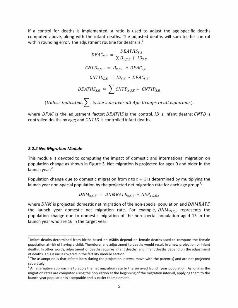
If a control for deaths is implemented, a ratio is used to adjust the age-specific deaths computed above, along with the infant deaths. The adjusted deaths will sum to the control within rounding error. The adjustment routine for deaths is:1

𝐷𝐹𝐴𝐶𝑆,𝐸 = 𝐷𝐸𝐴𝑇𝐻𝑆𝑆,𝐸

∑ 𝐷𝑥,𝑆,𝐸 + 𝐼𝐷𝑆,𝐸

𝐶𝑁𝑇𝐷𝑥,𝑆,𝐸 = 𝐷𝑥,𝑆,𝐸 ∗ 𝐷𝐹𝐴𝐶𝑆,𝐸

𝐶𝑁𝑇𝐼𝐷𝑆,𝐸 = 𝐼𝐷𝑆,𝐸 ∗ 𝐷𝐹𝐴𝐶𝑆,𝐸

𝐷𝐸𝐴𝑇𝐻𝑆𝑆,𝐸 ≈ ∑ 𝐶𝑁𝑇𝐷𝑥,𝑆,𝐸 + 𝐶𝑁𝑇𝐼𝐷𝑆,𝐸

(𝑈𝑛𝑙𝑒𝑠𝑠 𝑖𝑛𝑑𝑖𝑐𝑎𝑡𝑒𝑑, ∑. 𝑖𝑠 𝑡ℎ𝑒 𝑠𝑢𝑚 𝑜𝑣𝑒𝑟 𝑎𝑙𝑙 𝐴𝑔𝑒 𝐺𝑟𝑜𝑢𝑝𝑠 𝑖𝑛 𝑎𝑙𝑙 𝑒𝑞𝑢𝑎𝑡𝑖𝑜𝑛𝑠).

where 𝐷𝐹𝐴𝐶 is the adjustment factor; 𝐷𝐸𝐴𝑇𝐻𝑆 is the control, 𝐼𝐷 is infant deaths; 𝐶𝑁𝑇𝐷 is controlled deaths by age; and 𝐶𝑁𝑇𝐼𝐷 is controlled infant deaths.

2.2.2 Net Migration Module

This module is devoted to computing the impact of domestic and international migration on population change as shown in Figure 3. Net migration is projected for ages 0 and older in the launch year.2

Population change due to domestic migration from 𝑡 to 𝑡 + 1 is determined by multiplying the launch year non-special population by the projected net migration rate for each age group3:

𝐷𝑁𝑀𝑥,𝑆,𝐸 = 𝐷𝑁𝑀𝑅𝐴𝑇𝐸𝑥,𝑆,𝐸 ∗ 𝑁𝑆𝑃𝑥,𝑆,𝐸,𝑡

where 𝐷𝑁𝑀 is projected domestic net migration of the non-special population and 𝐷𝑁𝑀𝑅𝐴𝑇𝐸 the launch year domestic net migration rate. For example, 𝐷𝑁𝑀15,𝑆,𝐸 represents the population change due to domestic migration of the non-special population aged 15 in the launch year who are 16 in the target year.

1 Infant deaths determined from births based on ASBRs depend on female deaths used to compute the female

population at-risk of having a child. Therefore, any adjustment to deaths would result in a new projection of infant deaths. In other words, adjustment of deaths requires infant deaths, and infant deaths depend on the adjustment of deaths. This issue is covered in the fertility module section. 2 The assumption is that infants born during the projection interval move with the parent(s) and are not projected

separately. 3 An alternative approach is to apply the net migration rate to the survived launch year population. As long as the

migration rates are computed using the population at the beginning of the migration interval, applying them to the launch year population is acceptable and is easier to implement.

6

Figure 3: Net Migration Module

Domestic Net Migration

International Net Migration

If a control for domestic net migration is implemented, the Plus-Minus method is used to adjust the age-specific domestic net migration computed above. Unlike deaths, domestic net migration can have positive and negative values across age groups. In this case, two adjustment factors should be used to account for the positive and negative values separately. The Plus-Minus method will also work when the domestic net migration has the same sign for every age group. The adjusted domestic net migration will sum to the control within rounding error. The adjustment routine for domestic net migration is:

Launch Year Non-Special

Population Age (x)

Net Migration

Age (x+1)

Net Migration

Rates Age (x)

Net Migration

Control

Net Migration

Age (x)

Net Migration Allocation

Factors Age (x)

7

𝐴𝐵𝑆𝑈𝑀𝑆,𝐸 = ∑|𝐷𝑁𝑀𝑥,𝑆,𝐸|

𝑆𝑈𝑀𝑆,𝐸 = ∑ 𝐷𝑁𝑀𝑥,𝑆,𝐸

𝑃𝐹𝐴𝐶𝑆,𝐸 = 𝐴𝐵𝑆𝑈𝑀𝑆,𝐸 + (𝐷𝑁𝐸𝑇𝑀𝐼𝐺𝑆,𝐸 – 𝑆𝑈𝑀𝑆,𝐸)

𝐴𝐵𝑆𝑈𝑀𝑆,𝐸

𝑁𝐹𝐴𝐶𝑆,𝐸 = 𝐴𝐵𝑆𝑈𝑀𝑆,𝐸 – (𝐷𝑁𝐸𝑇𝑀𝐼𝐺𝑆,𝐸 – 𝑆𝑈𝑀𝑆,𝐸)

𝐴𝐵𝑆𝑈𝑀𝑆,𝐸

𝐼𝐹 𝐷𝑁𝑀𝑥,𝑆,𝐸 ≥ 0 𝑡ℎ𝑒𝑛 𝐶𝑁𝑇𝐷𝑁𝑀𝑥,𝑆,𝐸 = 𝐷𝑁𝑀𝑥,𝑆,𝐸 ∗ 𝑃𝐹𝐴𝐶𝑆,𝐸

𝐼𝐹 𝐷𝑁𝑀𝑥,𝑆,𝐸 < 0 𝑡ℎ𝑒𝑛 𝐶𝑁𝑇𝐷𝑁𝑀𝑥,𝑆,𝐸 = 𝐷𝑁𝑀𝑥,𝑆,𝐸 ∗ 𝑁𝐹𝐴𝐶𝑆,𝐸

𝐷𝑁𝐸𝑇𝑀𝐼𝐺𝑆,𝐸 ≈ ∑ 𝐶𝑁𝑇𝐷𝑁𝑀𝑥,𝑆,𝐸

where 𝐴𝐵𝑆𝑈𝑀 is sum of the absolute value of the uncontrolled domestic net migration estimates; 𝑆𝑈𝑀 is sum of the uncontrolled domestic net migration estimates; 𝐷𝑁𝐸𝑇𝑀𝐼𝐺 is the control; 𝑃𝐹𝐴𝐶 is the adjustment factor for positive values; and 𝑁𝐹𝐴𝐶 is the adjustment factor for negative values.

International net migration is projected differently than domestic net migration. Instead of international net migration rates, allocation factors are used to distribute the international net migration control to age groups. The factors represent the proportion of the projected international migration in each age group. If no control is supplied, the international migration projection will be zero. The projection of international net migration is:

𝐼𝑓 𝐼𝑁𝐸𝑇𝑀𝐼𝐺𝑆,𝐸 = 0 𝑡ℎ𝑒𝑛 𝐼𝑁𝑀𝑥,𝑆,𝐸 = 0

𝐼𝑓 𝐼𝑁𝐸𝑇𝑀𝐼𝐺𝑆,𝐸 ≠ 0 𝑡ℎ𝑒𝑛 𝐼𝑁𝑀𝑥,𝑆,𝐸 = 𝐼𝑁𝐸𝑇𝑀𝐼𝐺𝑆,𝐸 ∗ 𝐴𝐹𝐴𝐶𝑥,𝑆,𝐸

𝐼𝑁𝐸𝑇𝑀𝐼𝐺𝑆,𝐸 ≈ ∑ 𝐼𝑁𝑀𝑥,𝑆,𝐸

where 𝐼𝑁𝐸𝑇𝑀𝐼𝐺 is the control; 𝐼𝑁𝑀 is projected international migration; and 𝐴𝐹𝐴𝐶 isinternational migration age allocation factor.

2.2.3 Fertility Module

The fertility module is devoted to projecting births and infant deaths during the projection interval and the population age 0 in the target year for males and female as shown in Figure 4.

8

Figure 4: Fertility Module

This is accomplished in three steps. First, the at-risk female population by age is multiplied by the launch year ASBRs; these results are summed to obtain total births (at-risk means females of childbearing age). Second, total births are allocated between males and females using proportions. Finally, using infant survival rates, births are survived to obtain the projection for age 0 and infant deaths. These computations are:

𝐴𝐷𝐽𝐴𝑆𝐵𝑅𝑥,𝐸,𝑡 =(𝐴𝑆𝐵𝑅𝑥,𝐸,𝑡 + 𝐴𝑆𝐵𝑅𝑥+1,𝐸,𝑡)

2 (𝑥 = 14 𝑡𝑜 44)

Launch Year Female

Non-Special

Population Age (x)

Female deaths

Age (x)

Female Net Migration

Age (x)

At-Risk Female

Population Age (x)

Births by Age of

Mother

Total Births

Total Births by Sex

of Child

Projected Population

by Sex Age 0

Adjusted Age-Specific

Birth Rates (ASBRs)

(x+(x+1))/2

Allocation Factor

Infant Survival Rates

9

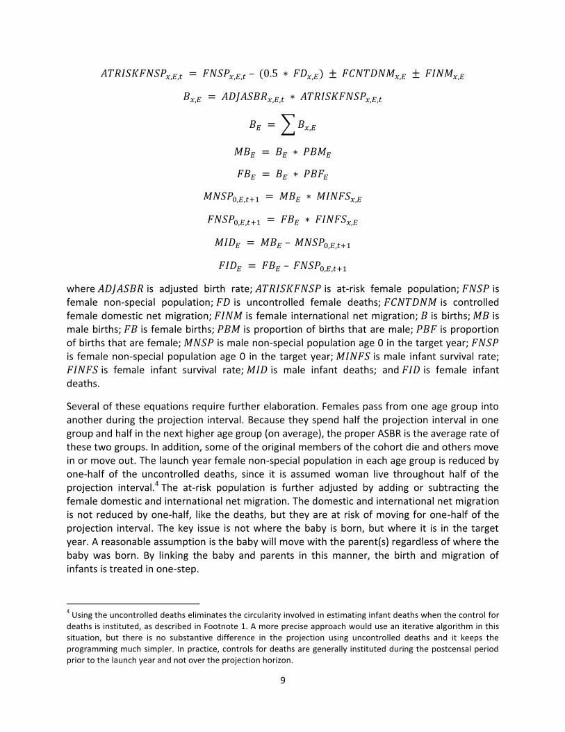
𝐴𝑇𝑅𝐼𝑆𝐾𝐹𝑁𝑆𝑃𝑥,𝐸,𝑡 = 𝐹𝑁𝑆𝑃𝑥,𝐸,𝑡 – (0.5 ∗ 𝐹𝐷𝑥,𝐸) ± 𝐹𝐶𝑁𝑇𝐷𝑁𝑀𝑥,𝐸 ± 𝐹𝐼𝑁𝑀𝑥,𝐸

𝐵𝑥,𝐸 = 𝐴𝐷𝐽𝐴𝑆𝐵𝑅𝑥,𝐸,𝑡 ∗ 𝐴𝑇𝑅𝐼𝑆𝐾𝐹𝑁𝑆𝑃𝑥,𝐸,𝑡

𝐵𝐸 = ∑ 𝐵𝑥,𝐸

𝑀𝐵𝐸 = 𝐵𝐸 ∗ 𝑃𝐵𝑀𝐸

𝐹𝐵𝐸 = 𝐵𝐸 ∗ 𝑃𝐵𝐹𝐸

𝑀𝑁𝑆𝑃0,𝐸,𝑡+1 = 𝑀𝐵𝐸 ∗ 𝑀𝐼𝑁𝐹𝑆𝑥,𝐸

𝐹𝑁𝑆𝑃0,𝐸,𝑡+1 = 𝐹𝐵𝐸 ∗ 𝐹𝐼𝑁𝐹𝑆𝑥,𝐸

𝑀𝐼𝐷𝐸 = 𝑀𝐵𝐸 – 𝑀𝑁𝑆𝑃0,𝐸,𝑡+1

𝐹𝐼𝐷𝐸 = 𝐹𝐵𝐸 – 𝐹𝑁𝑆𝑃0,𝐸,𝑡+1

where 𝐴𝐷𝐽𝐴𝑆𝐵𝑅 is adjusted birth rate; 𝐴𝑇𝑅𝐼𝑆𝐾𝐹𝑁𝑆𝑃 is at-risk female population; 𝐹𝑁𝑆𝑃 is female non-special population; 𝐹𝐷 is uncontrolled female deaths; 𝐹𝐶𝑁𝑇𝐷𝑁𝑀 is controlled female domestic net migration; 𝐹𝐼𝑁𝑀 is female international net migration; 𝐵 is births; 𝑀𝐵 is male births; 𝐹𝐵 is female births; 𝑃𝐵𝑀 is proportion of births that are male; 𝑃𝐵𝐹 is proportion of births that are female; 𝑀𝑁𝑆𝑃 is male non-special population age 0 in the target year; 𝐹𝑁𝑆𝑃 is female non-special population age 0 in the target year; 𝑀𝐼𝑁𝐹𝑆 is male infant survival rate; 𝐹𝐼𝑁𝐹𝑆 is female infant survival rate; 𝑀𝐼𝐷 is male infant deaths; and 𝐹𝐼𝐷 is female infant deaths.

Several of these equations require further elaboration. Females pass from one age group into another during the projection interval. Because they spend half the projection interval in one group and half in the next higher age group (on average), the proper ASBR is the average rate of these two groups. In addition, some of the original members of the cohort die and others move in or move out. The launch year female non-special population in each age group is reduced by one-half of the uncontrolled deaths, since it is assumed woman live throughout half of the projection interval.4 The at-risk population is further adjusted by adding or subtracting the female domestic and international net migration. The domestic and international net migration is not reduced by one-half, like the deaths, but they are at risk of moving for one-half of the projection interval. The key issue is not where the baby is born, but where it is in the target year. A reasonable assumption is the baby will move with the parent(s) regardless of where the baby was born. By linking the baby and parents in this manner, the birth and migration of infants is treated in one-step.

4 Using the uncontrolled deaths eliminates the circularity involved in estimating infant deaths when the control for

deaths is instituted, as described in Footnote 1. A more precise approach would use an iterative algorithm in this situation, but there is no substantive difference in the projection using uncontrolled deaths and it keeps the programming much simpler. In practice, controls for deaths are generally instituted during the postcensal period prior to the launch year and not over the projection horizon.

10

If a control for births is implemented, it replaces the total births determined using ASBRs and the at-risk female population. The controlled births are split into males and females, survived to age zero in the target year, and used to compute infant deaths based on the equations shown above.

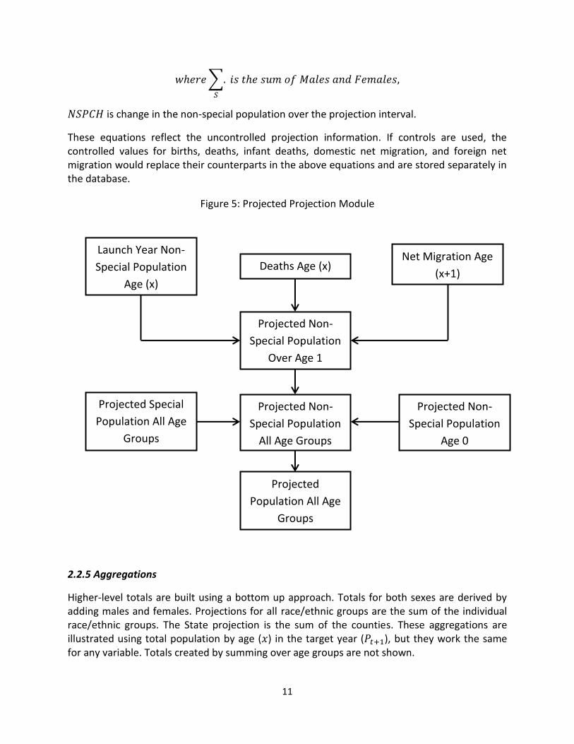
2.2.4 Projected Population Module

The projected population module combines the launch year non-special population with the results from the fertility, mortality, and net migration modules to develop the target year non-special projection by age. The special population projection is then added to complete the projection process as shown in Figure 5. The default for special population is to hold it constant at launch year values, but an independent projection can be defined for any year. The equations for this module are:

𝑁𝑆𝑃0,𝑆,𝐸,𝑡+1 = 𝐵𝑆,𝐸 – 𝐼𝐷𝑆,𝐸 𝐴𝑔𝑒 0

𝑁𝑆𝑃𝑥,𝑆,𝐸,𝑡+1 = 𝑁𝑆𝑃𝑥,𝑆,𝐸,𝑡 ± 𝐷𝑁𝑀𝑥,𝑆,𝐸 ± 𝐼𝑁𝑀𝑥,𝑆,𝐸 (𝑥 = 1 𝑡𝑜 85+)

𝑆𝑃𝑥,𝑆,𝐸,𝑡+1 = 𝑆𝑃𝑥,𝑆,𝐸 𝐷𝑒𝑓𝑎𝑢𝑙𝑡 (𝑥 = 0 𝑡𝑜 85+)

𝑃0,𝑆,𝐸,𝑡+1 = 𝑁𝑆𝑃0,𝑆,𝐸,𝑡+1 + 𝑆𝑃𝑥,𝑆,𝐸,𝑡+1 𝐴𝑔𝑒 0

𝑃𝑥,𝑆,𝐸,𝑡+1 = 𝑁𝑆𝑃𝑥,𝑆,𝐸,𝑡+1 + 𝑆𝑆𝑃𝑥,𝑆,𝐸,𝑡+1 (𝑥 = 1 𝑡𝑜 85+)

𝑁𝑆𝑃 is non-special population; 𝐵 is births, 𝐼𝐷 is infant deaths; 𝐷𝑁𝑀 is domestic net migration; 𝐼𝑁𝑀 is international net migration; 𝑆𝑃 is special population; 𝑃 is total population.

The components of population change are computed by aggregating the non-special population, deaths, and domestic and international net migration over age groups along with the projection of births. Components of change are computed for males, females, and both sexes as follows:

𝐷𝑆,𝐸 = ∑ 𝐷𝑥,𝑆,𝐸 + 𝐼𝐷𝑆,𝐸 (𝑥 = 1 𝑡𝑜 85+)

𝐷𝑁𝑀𝑆,𝐸 = ∑ 𝐷𝑁𝑀𝑥,𝑆,𝐸

𝐼𝑁𝑀𝑆,𝐸 = ∑ 𝐼𝑁𝑀𝑥,𝑆,𝐸

𝑁𝑆𝑃𝐶𝐻𝑆,𝐸 = ∑ 𝑁𝑆𝑃𝑥,𝑆,𝐸,𝑡+1 – ∑ 𝑁𝑆𝑃𝑥,𝑆,𝐸,𝑡

𝑁𝑆𝑃𝐶𝐻𝑆,𝐸 = 𝐵𝑆,𝐸 – 𝐷𝑆,𝐸 ± 𝐷𝑁𝑀𝑆,𝐸 ± 𝐷𝑁𝑀𝑆,𝐸

𝑁𝑆𝑃𝐶𝐻𝐸 = ∑ 𝐵𝑆,𝐸

𝑆

– 𝐷𝑆,𝐸 ± ∑ 𝐷𝑁𝑀𝑥,𝑆,𝐸

𝑆

± ∑ 𝐷𝑁𝑀𝑥,𝑆,𝐸

𝑆

11

𝑤ℎ𝑒𝑟𝑒 ∑.

𝑆

𝑖𝑠 𝑡ℎ𝑒 𝑠𝑢𝑚 𝑜𝑓 𝑀𝑎𝑙𝑒𝑠 𝑎𝑛𝑑 𝐹𝑒𝑚𝑎𝑙𝑒𝑠,

𝑁𝑆𝑃𝐶𝐻 is change in the non-special population over the projection interval.

These equations reflect the uncontrolled projection information. If controls are used, the controlled values for births, deaths, infant deaths, domestic net migration, and foreign net migration would replace their counterparts in the above equations and are stored separately in the database.

Figure 5: Projected Projection Module

2.2.5 Aggregations

Higher-level totals are built using a bottom up approach. Totals for both sexes are derived by adding males and females. Projections for all race/ethnic groups are the sum of the individual race/ethnic groups. The State projection is the sum of the counties. These aggregations are illustrated using total population by age (𝑥) in the target year (𝑃𝑡+1), but they work the same for any variable. Totals created by summing over age groups are not shown.

Launch Year Non-

Special Population

Age (x)

Deaths Age (x) Net Migration Age

(x+1)

Projected Non-

Special Population

Over Age 1

Projected Special

Population All Age

Groups

Projected Non-

Special Population

All Age Groups

Projected Non-

Special Population

Age 0

Projected

Population All Age

Groups

12

The computations for individual areas (A, for State or counties) are:

𝑃𝑥,𝐸,𝐴,𝑡+1 = ∑ 𝑃𝑥,𝑆,𝐸,𝐴,𝑡+1

𝑆

𝑃𝑥,𝑆,𝐴,𝑡+1 = ∑ 𝑃𝑥,𝑆,𝐸,𝐴,𝑡+1

𝐸

𝑃𝑥,𝐴,𝑡+1 = ∑ 𝑃𝑥,𝑆,𝐴,𝑡+1

𝑆

These computations for the bottom up State projections (PS) are:

𝑃𝑥,𝑆,𝐸,𝑡+1𝑠 = ∑ 𝑃𝑥,𝑆,𝐸,𝐴,𝑡+1

𝐴

𝑃𝑥,𝐸,𝑡+1𝑠 = ∑ 𝑃𝑥,𝑆,𝐸,𝑡+1

𝑠

𝑆

𝑃𝑥,𝑆,𝑡+1𝑠 = ∑ 𝑃𝑥,𝑆,𝐸,𝑡+1

𝑠

𝐸

𝑃𝑥,𝑡+1𝑠 = ∑ 𝑃𝑥,𝑆,𝑡+1

𝑠

𝑆

3. DATA INPUTS

Launch Year populations, both Total and Special (i.e. military personnel and dependents, prisoners, college students in dorms), form the starting point of a projection series, and various rates and proportions are used to compute the components of change. With the exception of the Launch Year total population, all of the data elements described below can be modified to reflect changing conditions during the projection series.

13

3.1 Population

The Launch Year total population is stratified by age, sex, and 6 race/ethnic groups. Each sex and race/ethnic group is arrayed into 85 single-year ages, from age 0 to age 84, and a final group ages 85 and over. The Special Population is stratified the same way as the Total Population. Special Populations complicate the projection process because their change is not determined by the same factors that affect fertility, mortality, and migration; consequently, they often follow trends that differ from the rest of the population and often have different demographic characteristics as well. These demographic differences can have a substantial impact on the projection of the components of change. Another characteristic of special populations is they often do not age in place as other population groups; therefore, their age structure may remain relatively stable over time.

3.2 Survival Rates

Survival rates are used to compute deaths and are derived from a life table. In a single-year model, the survival rate represents probability of a cohort surviving from one year to the next. Its complement is the probability of dying. One-year survival rates are needed for each age, sex, and race/ethnic group. An additional survival rate is required to compute infant deaths. This makes 87 survival rates for each sex and race/ethnic group in the model.

3.3 Fertility Rates

Age-Specific Birth Rates (ASBR) for individual ages from 15 to 44 are used to project births. A schedule of ASBRs is needed for each race/ethnic group. When there is no control, the birth rates are applied to the Launch Year female population adjusted for deaths and migration during the projection horizon. The proportions of births that are male (PBM) and female (PBF) are used to project male and female births respectively.

3.4 Migration Rates

Net migration rates for ages 1+, sex, and race/ethnic group are used to project domestic migration. Net migration rates use the local area (State or County) population as the population at risk in the denominator. These rates are based on the population at the beginning of the migration interval. The domestic migration projections are derived by applying these rates to the Launch Year population.

The projection of international net migration uses allocation factors by single year of age, which represents the share of the total net international migration; therefore, these factors sum to 1.0 over all ages. Separate factors for each sex and race/ethnic group are used in conjunction with sex and race/ethnic group-specific controls to project international migration.

3.4 Controls

Controls were employed for total net migration. Since age-specific net migration can be negative, zero, or positive, a two-factor controlling routine was used. For adjusting deaths, a single-factor routine was sufficient.

14

4. THE MODELING PROCESS

4.1 Fertility Rates

Fertility rates by mother's age group, race/ethnicity and county of residence were computed for the year centered on the 2010 Census Date (October 1, 2009 - September 30, 2010). Rates for the Balance of State (i.e. all counties excluding Maricopa, Pinal and Pima) were also computed.

The rates excluded the <15 and 45+ age groups. However, the births by females aged <15 were included in the 15-19 age group while the births by females aged 45+ were included in the 40-44 age group, with no adjustments made to the base populations of the rates.

Total Fertility Rates (TFRs) by county and race/ethnicity were also computed. Comparisons were made between counties and state, race/ethnic groups, and the total population.

Out of 150 combinations (i.e. 15 counties x 10 race/ethnic groups), nearly three-quarters (110) had less than 150 births. Birth rates calculated for these combinations were not reliable. Due to a mismatch of race/ethnic grouping between Census and birth data, the state-level rates were not applicable, either. Therefore, a substitution scheme was developed and applied accordingly.

Age-specific birth rates were computed for White Non-Hispanics (White NH) and Other Non-Hispanics (Other NH) combined. These rates were substituted for the White NH group and the Other NH group. Both the White Hispanic group and Other Hispanic group used the rates computed for Hispanics of any race. For the remaining 6 race/ethnic groups, the ratios of Non-Hispanic ASBR to Total ASBR, or the ratios of Hispanic ASBR to Total ABSR (depending on the Hispanic origin) were applied to the ASBRs of each race to obtain the new race/ethnic rates. The H and NH ratios were based on the total population (all races) ASBR.

The rates obtained from the substitution for all race/ethnic groups were applied to the female non-special population as of July 1, 2010 to estimate births in Fiscal Year 2011. Using the actual births and projected births, an adjustment factor was computed and applied to the rates from the substitution to obtain the new ASBRs and TFRs. This adjustment is a calibration process that ensures the fertility rates closely produce the number of births that occur in reality. Calibration was performed for each county and Arizona5.

4.1.1 Projection of Fertility Rates

To project the ASBRs over the projection horizon, historical US fertility trends were studied. US ASBRs and TFRs between 1990 and 2010 were collected for five race/ethnic groups (White NH, Black NH, American Indian or Alaska Native, Asian or Pacific Islander, and Hispanic (of any

5 One set of state rates were computed. These state rates were used for all counties but were calibrated to actual

county births for FY2011.

15

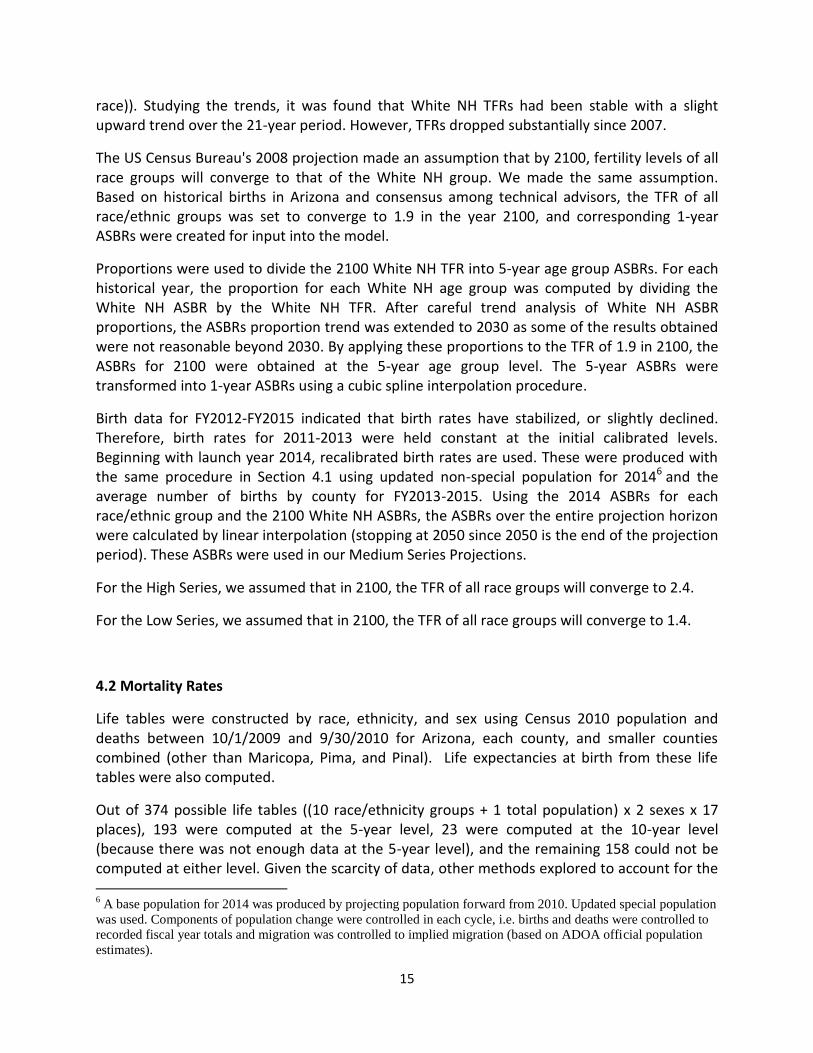
race)). Studying the trends, it was found that White NH TFRs had been stable with a slight upward trend over the 21-year period. However, TFRs dropped substantially since 2007.

The US Census Bureau's 2008 projection made an assumption that by 2100, fertility levels of all race groups will converge to that of the White NH group. We made the same assumption. Based on historical births in Arizona and consensus among technical advisors, the TFR of all race/ethnic groups was set to converge to 1.9 in the year 2100, and corresponding 1-year ASBRs were created for input into the model.

Proportions were used to divide the 2100 White NH TFR into 5-year age group ASBRs. For each historical year, the proportion for each White NH age group was computed by dividing the White NH ASBR by the White NH TFR. After careful trend analysis of White NH ASBR proportions, the ASBRs proportion trend was extended to 2030 as some of the results obtained were not reasonable beyond 2030. By applying these proportions to the TFR of 1.9 in 2100, the ASBRs for 2100 were obtained at the 5-year age group level. The 5-year ASBRs were transformed into 1-year ASBRs using a cubic spline interpolation procedure.

Birth data for FY2012-FY2015 indicated that birth rates have stabilized, or slightly declined. Therefore, birth rates for 2011-2013 were held constant at the initial calibrated levels. Beginning with launch year 2014, recalibrated birth rates are used. These were produced with the same procedure in Section 4.1 using updated non-special population for 20146 and the average number of births by county for FY2013-2015. Using the 2014 ASBRs for each race/ethnic group and the 2100 White NH ASBRs, the ASBRs over the entire projection horizon were calculated by linear interpolation (stopping at 2050 since 2050 is the end of the projection period). These ASBRs were used in our Medium Series Projections.

For the High Series, we assumed that in 2100, the TFR of all race groups will converge to 2.4.

For the Low Series, we assumed that in 2100, the TFR of all race groups will converge to 1.4.

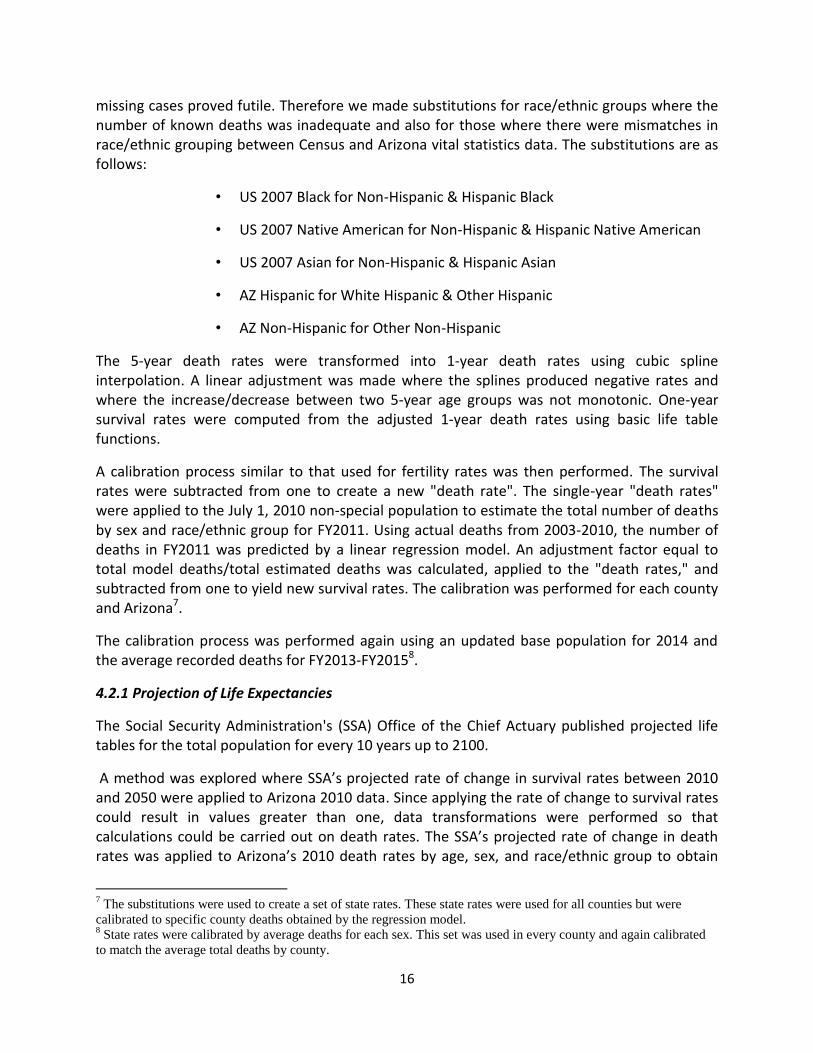
4.2 Mortality Rates

Life tables were constructed by race, ethnicity, and sex using Census 2010 population and deaths between 10/1/2009 and 9/30/2010 for Arizona, each county, and smaller counties combined (other than Maricopa, Pima, and Pinal). Life expectancies at birth from these life tables were also computed.

Out of 374 possible life tables ((10 race/ethnicity groups + 1 total population) x 2 sexes x 17 places), 193 were computed at the 5-year level, 23 were computed at the 10-year level (because there was not enough data at the 5-year level), and the remaining 158 could not be computed at either level. Given the scarcity of data, other methods explored to account for the 6 A base population for 2014 was produced by projecting population forward from 2010. Updated special population

was used. Components of population change were controlled in each cycle, i.e. births and deaths were controlled to

recorded fiscal year totals and migration was controlled to implied migration (based on ADOA official population

estimates).

16

missing cases proved futile. Therefore we made substitutions for race/ethnic groups where the number of known deaths was inadequate and also for those where there were mismatches in race/ethnic grouping between Census and Arizona vital statistics data. The substitutions are as follows:

• US 2007 Black for Non-Hispanic & Hispanic Black

• US 2007 Native American for Non-Hispanic & Hispanic Native American

• US 2007 Asian for Non-Hispanic & Hispanic Asian

• AZ Hispanic for White Hispanic & Other Hispanic

• AZ Non-Hispanic for Other Non-Hispanic

The 5-year death rates were transformed into 1-year death rates using cubic spline interpolation. A linear adjustment was made where the splines produced negative rates and where the increase/decrease between two 5-year age groups was not monotonic. One-year survival rates were computed from the adjusted 1-year death rates using basic life table functions.

A calibration process similar to that used for fertility rates was then performed. The survival rates were subtracted from one to create a new "death rate". The single-year "death rates" were applied to the July 1, 2010 non-special population to estimate the total number of deaths by sex and race/ethnic group for FY2011. Using actual deaths from 2003-2010, the number of deaths in FY2011 was predicted by a linear regression model. An adjustment factor equal to total model deaths/total estimated deaths was calculated, applied to the "death rates," and subtracted from one to yield new survival rates. The calibration was performed for each county and Arizona7.

The calibration process was performed again using an updated base population for 2014 and the average recorded deaths for FY2013-FY20158.

4.2.1 Projection of Life Expectancies

The Social Security Administration's (SSA) Office of the Chief Actuary published projected life tables for the total population for every 10 years up to 2100.

A method was explored where SSA’s projected rate of change in survival rates between 2010 and 2050 were applied to Arizona 2010 data. Since applying the rate of change to survival rates could result in values greater than one, data transformations were performed so that calculations could be carried out on death rates. The SSA’s projected rate of change in death rates was applied to Arizona’s 2010 death rates by age, sex, and race/ethnic group to obtain

7 The substitutions were used to create a set of state rates. These state rates were used for all counties but were

calibrated to specific county deaths obtained by the regression model. 8 State rates were calibrated by average deaths for each sex. This set was used in every county and again calibrated

to match the average total deaths by county.

17

death rates for 2011-2050. These death rates were converted back to survival rates. Unfortunately, this process did not provide good control over the target year life expectancies.

Therefore, the method used to project life expectancies relied on the numerical difference in SSA’s projections instead of the rate of change. In principle, the difference between SSA’s life expectancy in 2010 and 2050 was added to Arizona’s 2010 life expectancy to obtain the Arizona life expectancy in 2050. A problem arises given that SSA publishes life tables for the total population while Arizona’s projections are based on 10 race/ethnic groups, i.e. not every group will experience the same improvement in life expectancy as reported by SSA.

According to the Census Bureau's 2008 population projection, different race/ethnicity and sex groups are projected to have the following number of years in life expectancy improvement between 2010 and 2050:

Hispanic (of any race): Male 3.5, Female 2.6

Non-Hispanic Black: Male 8.9, Female 7.2

Non-Hispanic (all other races): Male 4.6, Female 4.2

These race/ethnicity groupings also do not correspond directly to those used in Arizona’s model, and it is difficult to reconcile these changes with those produced by the SSA. However, a useful pattern was observed; improvement in projected life expectancy is inversely related to the current life expectancy. If a group currently has a relatively low life expectancy, its projected improvement is relatively high. To respect this pattern, the projected improvement in life expectancy was adjusted (either upward or downward) based on current life expectancies of each race/ethnicity/sex group. That is, if a race/ethnicity/sex group's 2010 life expectancy were lower than the SSA's 2010 total population life expectancy, an upward adjustment was made; if the race/ethnicity/sex group's 2010 life expectancy were higher than the SSA's 2010 total population life expectancy, a downward adjustment was made. After some experimentation, the group adjustment was set to equal 1/4 of the difference between SSA's 2010 total population life expectancy and the Arizona race/ethnicity/sex group's 2010 life expectancy. To obtain the 2050 life expectancy for a particular group, the formula below was used.

2050 𝐿𝑖𝑓𝑒 𝐸𝑥𝑝𝑒𝑐𝑡𝑎𝑛𝑐𝑦 (𝐿𝐸) = 𝐴𝑍 2010 𝐿𝐸 𝑤𝑖𝑡ℎ 𝑆𝑢𝑏𝑠𝑡𝑖𝑡𝑢𝑡𝑖𝑜𝑛 & 𝐶𝑎𝑙𝑖𝑏𝑟𝑎𝑡𝑖𝑜𝑛 +

𝑆𝑆𝐴 𝐶ℎ𝑎𝑛𝑔𝑒 + 𝐺𝑟𝑜𝑢𝑝 𝐴𝑑𝑗𝑢𝑠𝑡𝑚𝑒𝑛𝑡

The previously calibrated survival rates were adjusted to match the 2050 life expectancies and were used as the final survival rates for 2050. Linear interpolation was used to produce the survival rates for 2011-2049. These survival rates were used for the 2012 Medium Series projections.

To obtain survival rates and life expectancies for the 2012 Low Series projections, the 2030 SSA life table was substituted for the 2050 life table. For the 2012 High Series projection, the 2070 SSA life table was substituted for the 2050 life table. The logic is that in the next 40 years, instead of making improvements in survival rates and life expectancies that SSA projected for

18

2050, improvements for the Low Series would only reach the level that SSA projected for 2030; improvements for the High Series would reach the level that SSA projected for 2070. The group adjustment for the Low Series was 1/5 and 1/3 for the High Series.

The updated calibration process in 2015 revealed that life expectancies had not changed in recent years. Because of this, the same survival rates that were developed in 2012 for the year 2050 were kept for the 2015 Low, Medium, and High series projections. Survival rates for 2016-2049 were obtained by linear interpolation beginning with the new calibrated survival rates.

4.3 Special Populations

For the projections model, military persons in Group Quarters (GQ), military persons in households and their dependents, people in adult correctional facilities, and college students in dormitories were treated as Special Population.

The number of military persons and their dependents not in GQ were estimated using the ACS 2008-2010 3-year data. The proportion of total population that is active military and their dependents was calculated. These proportions were applied to the launch year population to estimate the number of military and their dependents9. The resulting number was added to the Census 2010 Special Population and held constant for the projection horizon.

Some counties have a large number of college students who do not live in dorms and thus, were not accounted for in the Census 2010 special population. Also, the census special population was only available in 5-year age groups, causing more people to be distributed to ages 15-17 than there should be given that most college students are 18 and older. To more accurately reflect the student population, adjustments were made to the special population ages 17-30 for Coconino, Pima, Maricopa, and Arizona.

For Coconino and Pima, a method was devised to compare the census total population to the natural cohort of ages 17-30. The difference between the two is assumed to be special population. Specifically, a line was drawn from the census population of age 16 to age 31. This represented the natural cohort of residents in the county. For each year of age, the natural cohort was subtracted from the census population to obtain the estimated special population. All negative results were replaced with zero. The distribution of special population in Coconino and Pima combined was then used to redistribute the special population totals for ages 15-24 in Maricopa and Arizona.

Special population was updated in 2015 to account for growth in the college population, as evidenced by enrollment figures from four major universities in Arizona10. The annualized

9 ACS data is categorized by Public Use Microdata Areas (PUMA) which sometimes consist of more than one

county. Military and their dependents in the Gila+Pinal PUMA were assigned to Pinal. Military and their dependents

from the Cochise, Graham, Greenlee, and Santa Cruz PUMA were assigned to Cochise. 10

University of Arizona, Arizona State University, Northern Arizona University, and Embry-Riddle Aeronautical

University

19

growth rate from 2010-201411 for each university was applied to the Census dormitory population of the counties where each institution was located12. Arizona experienced its peak number of births in 2007, and these children would reach college age (18 years) in 2025. To account for this, the dormitory population was allowed to grow until 2025. From 2025-2050, special population of all ages was held constant. The growth in special population is in addition to net migration controls discussed in the following sections.

(Section 4.4 and all its sub-sections through 4.4.4.3 describe the methods used in the 2012 edition to set net migration controls. Section 4.5 describes revisions for the 2015 edition.)

4.4 Migration – Original 2012 Series

Development of net migration data inputs involved several steps. Controls for total net migration were developed using historical data, which were then subdivided into net foreign migration, net domestic migration, and the required race/ethnicity/sex/age groups. This process is depicted in Figure 6 and described in the following sections.

Figure 6: Development of Migration Controls

11

Special population for 2010-2014 was also updated using the growth rates. The updated figures were used to

calculate the base population in 2014 for calibration of vital rates and subsequently to produce the launch year

population of 2015. 12

Pima, Maricopa, Coconino, and Yavapai

Total Net Migration:

Decadal Control

Foreign Net Migration:

Annual Control

Domestic Net Migration:

Annual Control

Subdivision into

Race/Ethnicity/Sex

Subdivision into

Race/Ethnicity/Sex

Subdivision into Age

Using Distribution Rates

Controlled Migrants

Using Plus-Minus Method

Total Net Migration:

Annual Control

Uncontrolled Domestic

Migrants:

Race/Ethnicity/Sex/Age

Launch Year

Population

Net Domestic

Migration Rates

20

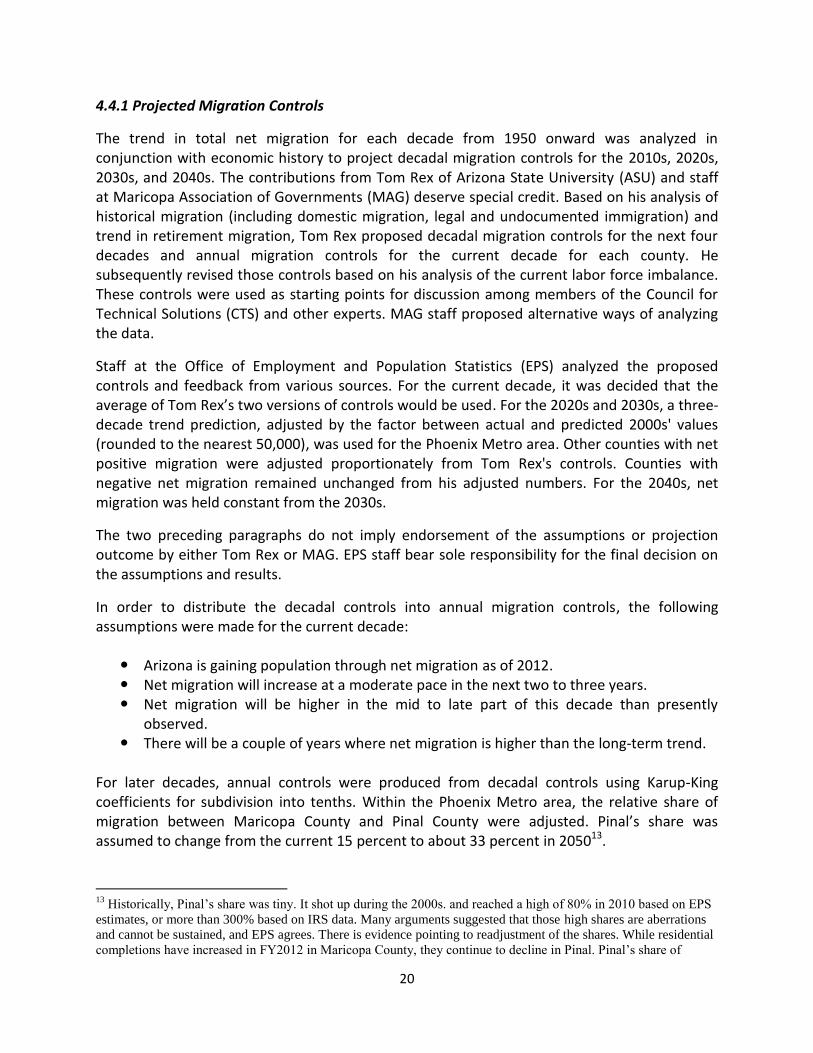
4.4.1 Projected Migration Controls

The trend in total net migration for each decade from 1950 onward was analyzed in conjunction with economic history to project decadal migration controls for the 2010s, 2020s, 2030s, and 2040s. The contributions from Tom Rex of Arizona State University (ASU) and staff at Maricopa Association of Governments (MAG) deserve special credit. Based on his analysis of historical migration (including domestic migration, legal and undocumented immigration) and trend in retirement migration, Tom Rex proposed decadal migration controls for the next four decades and annual migration controls for the current decade for each county. He subsequently revised those controls based on his analysis of the current labor force imbalance. These controls were used as starting points for discussion among members of the Council for Technical Solutions (CTS) and other experts. MAG staff proposed alternative ways of analyzing the data.

Staff at the Office of Employment and Population Statistics (EPS) analyzed the proposed controls and feedback from various sources. For the current decade, it was decided that the average of Tom Rex’s two versions of controls would be used. For the 2020s and 2030s, a three-decade trend prediction, adjusted by the factor between actual and predicted 2000s' values (rounded to the nearest 50,000), was used for the Phoenix Metro area. Other counties with net positive migration were adjusted proportionately from Tom Rex's controls. Counties with negative net migration remained unchanged from his adjusted numbers. For the 2040s, net migration was held constant from the 2030s.

The two preceding paragraphs do not imply endorsement of the assumptions or projection outcome by either Tom Rex or MAG. EPS staff bear sole responsibility for the final decision on the assumptions and results.

In order to distribute the decadal controls into annual migration controls, the following assumptions were made for the current decade:

Arizona is gaining population through net migration as of 2012. Net migration will increase at a moderate pace in the next two to three years. Net migration will be higher in the mid to late part of this decade than presently

observed. There will be a couple of years where net migration is higher than the long-term trend.

For later decades, annual controls were produced from decadal controls using Karup-King coefficients for subdivision into tenths. Within the Phoenix Metro area, the relative share of migration between Maricopa County and Pinal County were adjusted. Pinal’s share was assumed to change from the current 15 percent to about 33 percent in 205013.

13

Historically, Pinal’s share was tiny. It shot up during the 2000s. and reached a high of 80% in 2010 based on EPS

estimates, or more than 300% based on IRS data. Many arguments suggested that those high shares are aberrations

and cannot be sustained, and EPS agrees. There is evidence pointing to readjustment of the shares. While residential

completions have increased in FY2012 in Maricopa County, they continue to decline in Pinal. Pinal’s share of

21

Annual controls for each county and the state were separated into annual domestic controls and annual foreign controls. Foreign controls were calculated first and then subtracted from the total net migration controls to produce the domestic controls.

The Census Bureau’s preliminary projection of net foreign migration was used along with AZ data on legal permanent residents to project foreign migration controls. Two methods were used by the Census Bureau to project US foreign migration in 2060. Linear interpolation between 2010 and 2060 was used to estimate annual foreign migration for both methods, and an average was taken of the interpolated results. Arizona’s share of US legal permanent residents was then extrapolated from data compiled by the Department of Homeland Security and applied to the averaged Census projections to obtain annual foreign migration controls14. The extrapolation of Arizona’s share ran to 2030 and then remained constant until 2050 in the Medium series.

For the Low series, the current decade’s total net migration controls were set to 70 percent of

the Medium series (for positive controls) or to 130 percent (for negative controls). Subsequent

decades’ controls were assumed to equal the 1980s level (rounded to the nearest 50,000).

Arizona’s share of US foreign migration was assumed to stay constant at the 2011 level for the

entire projection horizon.

The High series adjusts the Medium series controls by 125 percent (for positive controls) or 75

percent (for negative controls). Subsequent decades used a five-decade trend to predict the

Phoenix Metro area (rounded to the nearest 50,000). Other counties with positive controls

were adjusted proportionately. Negative controls remained unchanged for the 2020s and were

set at 80 percent of the previous decade for the 2030s and 2040s. The trend of Arizona’s share of

US foreign migration was allowed to run to 2050.

4.4.2 Subdivision of County Migration Controls

After the annual migration controls were calculated, a procedure was established to subdivide those controls into the required 20 race/ethnicity/sex groups. The procedure followed for domestic migration and foreign migration were the same; the county total was proportionately split into 20 groups based on an assumed distribution. However, the distribution used for each type of migration differed.

ACS 5-year PUMS data for 2005-2010 were used to model the distribution of foreign migrants across the 20 groups. Originally, only data on ACS immigrants were used. However, these data produced distributions that did not coincide with other demographic information. Analysis was

residential completions in the metro area in FY2012 is 13%, down from 28% in FY2006. In the long run, however,

most people agree that Pinal still has potential. Thus, its share is allowed to go up over time. 14

Annual foreign migration controls were created at the state level. County shares, calculated from intercensal

estimates by EPS and the Census Bureau, were used to subdivide the state’s annual foreign migration controls.

22

then expanded to include all foreign born persons who entered Arizona in 2005 or later. These distributions made much more sense and were used to split the annual foreign migration control into smaller levels.

Domestic migration from several ACS 3- and 5-year PUMS were analyzed but also produced unusable distributions. The Census 2010 total population data provided a much more believable scenario and was used to distribute the annual domestic migration control for each county into smaller groups.

Adjustments to the domestic distribution were needed to more accurately capture the movement of Native Americans within the state. For Coconino and Navajo counties, the projected net migration was positive. However, it is expected that a net loss of Native Americans should occur based on past trends. To ensure that a net loss was realized for these two counties, a constant value for net outmigration was used. Because all other counties, except Maricopa, had very little movement of Native Americans, the proportion of migrants assigned to the Native American race groups was set to zero. The proportions of the remaining 18 race/ethnicity/sex groups were then adjusted to sum to 100 percent.

4.4.3 Net Foreign Migration Distribution Rates

Using 1995-2000 Census and 2007-2009 ACS migration data, proportionate distributions by

single year age groups for the 20 race/ethnic group/sex combinations were created. These

distribution rates were used to partition the net foreign migration controls into age groups.

Greater reliance was placed on the 1995-2000 Census data because of the greater variability

and unreasonable trends observed in the ACS data, especially for Blacks, Native Americans, and

Asians, when stratified by age, sex, and Hispanic origin.

The 1995-2000 data did not contain the 1-4 age group. So the ACS 2007-2009 data were used to

estimate the 1-4 age group for 1995-2000 using the ratio of the shares of 1-4 to 5-9 from the

total net foreign migration. Where possible, the race-specific ratio of the shares was used to

estimate the proportion in each race group. The resulting proportionate distributions were

adjusted to sum to one.

State-level factors were used to create the distributions for Hispanics and Non-Hispanics, males

and females within these race/ethnic categories, and to allocate 5-year age groups into single

year of age. These state factors were used for Maricopa, Pima, Pinal, and the balance of the

State because of data limitations and they provided more consistency in the distributions across

geographic areas. The steps below detail how the foreign distribution rates were computed.

1. The proportionate distributions by 5-year age groups were averaged for each race from

the Census and ACS data.

23

2. The age distribution for each race was split into initial Hispanic and non-Hispanic origin

distributions using the age-specific ratios of the Hispanic to total share and non-Hispanic

to total share. The same ratios were used for each race group given data limitations and

also because they adequately captured the tendency for Hispanic foreign migrants to be

younger than non-Hispanic foreign migrants. They were adjusted to sum to one.

3. The age distribution for Hispanics was split into initial male and female distributions

using the age-specific ratios of the male Hispanic to Total Hispanic share and female

Hispanic to Total Hispanic share. The same ratios are used for Hispanics for each race

group given data limitations and because they adequately captured the variation by sex

in the Hispanic population. They were adjusted to sum to one.

4. The age distribution for non-Hispanics was split into initial male and female distributions

using the age-specific ratios of the Male non-Hispanic to Total non-Hispanic share and

female non-Hispanic to total non-Hispanic share. The same ratios are used for non-

Hispanics for each race group given data limitations, and they adequately captured the

variation by sex in the non-Hispanic population. They were adjusted to sum to one.

5. The 5-year shares were then allocated into single years using the proportion of each 5-

year age group contained in its single year of age. The factors were based on the net

foreign migrants from 1995-2000.

Net foreign migration distribution rates were used twice in the development of the total net

migration data inputs. First, the rates were used in the process of developing the net domestic

migration rates. They were applied to an annualized foreign migration estimate and subtracted

from the annualized total implied net migration to yield annualized net domestic migration.

Second, the rates were directly applied to the projected foreign net migration controls up to

and including 2050.

4.4.4 Net Domestic Migration Rates

Calculation of the net domestic migration rates was an incredibly detailed process. Two distinct sets of rates were produced using two distinct methods. The average rates of both sets were used in the model. The first method required the estimation of annualized implied total net migration, annualized foreign net migration, and annualized net domestic migration. Simply described, the net domestic migration rate is produced using the formula

𝐷𝑜𝑚𝑒𝑠𝑡𝑖𝑐 𝑀𝑖𝑔𝑟𝑎𝑡𝑖𝑜𝑛 𝑅𝑎𝑡𝑒 =(𝐴𝑛𝑛𝑢𝑎𝑙𝑖𝑧𝑒𝑑 𝑇𝑜𝑡𝑎𝑙 𝑁𝑒𝑡 𝑀𝑖𝑔𝑟𝑎𝑛𝑡𝑠 − 𝐴𝑛𝑛𝑢𝑎𝑙𝑖𝑧𝑒𝑑 𝐹𝑜𝑟𝑒𝑖𝑔𝑛 𝑀𝑖𝑔𝑟𝑎𝑛𝑡𝑠)

𝑃𝑜𝑝𝑢𝑙𝑎𝑡𝑖𝑜𝑛 𝐵𝑎𝑠𝑒

The second method made use of the migration information from Census 2000 for the period 1995-2000. Details of each method are in the following sections.

24

4.4.4.1 Implied Migration Method

Due to the lack of accurate direct migration data, implied migration for the decade was computed using both 2010 and 2000 Census Populations, Births, Deaths, and the formula

𝐼𝑚𝑝𝑙𝑖𝑒𝑑 𝑀𝑖𝑔𝑟𝑎𝑡𝑖𝑜𝑛 = ∆𝑃𝑜𝑝𝑢𝑙𝑎𝑡𝑖𝑜𝑛 − ∆𝐵𝑖𝑟𝑡ℎ𝑠 + ∆𝐷𝑒𝑎𝑡ℎ𝑠

where ∆ is the change between 2000 Census and 2010 Census dates.

The steps below delineate how implied migration was calculated:

1. For each race/ethnic/sex group, implied net migration was calculated for the state,

Maricopa, Pima, Pinal, and Balance of State.

2. The ethnicity of intercensal births was adjusted to compensate for suspected differential

classification of Hispanic births. The adjustment was guided by historical data from

single year ACS PUMS from 2000-2010.

3. A ratio adjustment was performed on the Census 2010 population under 10 years of age

to reflect undercounting of young children. The ratio compares the population of

children under 10 from the Census Bureau’s Demographic Analysis to the Census 2010

population.

4. The implied net migration over 10 years was then annualized.

5. The estimated net foreign migrants are subtracted from the annualized net migration to

obtain the annualized domestic net migration.

6. A population denominator is calculated and used to produce a net domestic migration

rate.

4.4.4.2 Census Migrants 1995-2000 Method

Using the tabulation of migrants from Census 2000, state-level factors were used to create 5-year migration rates for Hispanics and Non-Hispanics and males and females within these race/ethnic categories. These state factors were used for Maricopa, Pima, Pinal, and the Balance of the State because of data limitations and to provide more consistency in the age-specific rates across geographic areas. The detailed steps are as follows:

1. Estimated age-specific rates for Hispanics and non-Hispanics using the age-specific ratios

of the Hispanic to total rate and non-Hispanic to total rate. The same ratios were used

for each race group given data limitations, and they adequately captured the tendency

for Hispanic domestic migrants to be younger do not have increased rates in the

retirement ages compared to non-Hispanic domestic migrants.

2. The age-specific rate for Hispanics was split into male and female rates using age-

specific ratios of the Male Hispanic to Total Hispanic rate and female Hispanic to Total

Hispanic rate. The same ratios were used for Hispanics for each race group given data

25

limitations, and they adequately captured the variation by sex in the Hispanic

population.

3. The age-specific rates for non-Hispanics were split into initial male and female rates

using age-specific ratios of the Male non-Hispanic to Total non-Hispanic rate and female

non-Hispanic to Total non-Hispanic rate. The same ratios were used for non-Hispanics

for each race group given data limitations, and they adequately captured the variation

by sex in the non-Hispanic population.

4. Using cubic spline interpolation, the 5-year age group rates were interpolated into single

year ages.

5. Initial estimate of the net migration by age by each sex and race/ethnic group was

generated using the Census 2010 data, and the Plus-Minus method was used to adjust

the rates so they match the calibration control. The same adjustment factor(s) was

applied to each sex and race/ethnic group.

4.4.4.3 Adjustments to Net Domestic Migration Rates

The assumption was that averaging the two sets of rates above would produce more reasonable migration rates than using any one method alone. However, even after averaging, tests revealed that further adjustments were needed.

Three types of adjustments were made. The first, and the simplest, was applied to ages 70 and older in all counties and the state. All positive migration rates for ages 70 and older were replaced with zero. This adjustment was needed because implied migration showed net outmigration occurring in older ages, which was not reflected by the averaged rates. Net outmigration among the very old is widely recognized among the senior living community. The hypothesis is that as out-of-state retirees become older and frailer, some of them move out of state to be closer to their children. This is solidly supported by migration figures implied by decennial census data and death statistics.

The second adjustment was applied to five counties15 for the college-age population and was needed because the “balance of state” migration rates did not adequately capture the out-migration in this age band. The adjustment was based on survival analysis. The population for 2009 was estimated using the 10-year migration rate between age seven and seventeen16. An annual migration rate was then calculated using the Census 2010 population and estimated 2009 population and replaced the averaged rates.

15

Apache, Gila, La Paz, Navajo, and Santa Cruz 16

The method assumes that all changes in the population are due to migration. Deaths are not considered as they are

a small part of the population change for 7-17 year-olds.

26

The last adjustment was made to ages 37+ in Gila and 45+ in La Paz. Rates were recalculated by annualizing the implied net migration between Census 2000 and Census 2010 and dividing by a population base. This was needed because the age patterns of migration in these counties were demonstrably different than those of the “balance of county.” The adjustment was also based on survival analysis.

4.5 Migration – 2015 Update

Since the 2012 projections series was published, three more years of migration data have been

accumulated. Implied migration for 2013-2015 suggested that for Metro Phoenix and Arizona

as a whole, the 2012 Medium Series assumptions were well within range of reality. For these

reasons, it was decided that long-term migration assumptions would not be changed unless

recent data warrant a reconsideration. No change was made to the 2012 Medium Series

migration controls for 2020-2050 in eight counties. Adjustments were, however, made to long-

term migration levels in seven counties and to short-term migration (2016-2019) for all

counties.

The implied migration for Cochise, Mohave, and Navajo was consistently lower than the 2012

series assumptions for 2013-2015. For these three counties, the Low Series assumptions from

2012 were adopted as the new Medium Series controls for 2020-2050.

Based on historical data spanning about 40 years, the long-term assumptions for Coconino,

Pima, and Yavapai counties also needed adjustment. Implied migration in Coconino was higher

than assumed and needed an upward adjustment. Pima and Yavapai needed downward

adjustment. The long-term migration for these counties was set to the average annual

migration experienced over the last 35 years. This adjustment placed Pima’s migration trend

near the middle of the 2012 medium and low series. Yavapai’s migration was placed slightly

below the halfway point between the 2012 medium and low series. Coconino’s long-term

annual migration was nearly doubled.

When migration controls were developed in 2012, migration for Metro Phoenix was projected

and then split up between Maricopa and Pinal. This split between the two counties has been

adjusted in the new series. Pinal’s share of migration was assumed to stay at 15 percent of

Metro Phoenix until 2020 and then steadily grow to 30 percent in 2050 based on trends in

residential completions, implied migration, IRS migration data, and discussions with MAG and

CAG.

A short-term cycle of increased migration from 2016-2019 was assumed in the 2012 series. In

this update, the cycle was removed from all counties. All feedback received by EPS has been in

support of removing this cycle, which seems unlikely to occur in the present economic

27

environment. New migration controls for 2016-2019 were produced using a 3rd or 4th order

polynomial fit from 2015 implied migration to assumed long-term controls for 2020-2025 for all

counties except Pinal.

5. ACKNOWLEDGMENTS

The EPS staff would like to thank the following people for their contributions to the projections process. They devoted many hours of discussion and data analysis and provided guidance for model design that resulted in high quality data inputs and results. The affiliation listed for each person is as of the time of their contribution and may or may not be current.

Current and Past Members of the Council for Technical Solutions:

Anubhav Bagley, MAG Dr. Robert Carreira, Cochise College Dr. Alberta Charney, U of A Tracy Clark, ADOT Chris Fetzer, NACOG Mark Griffin, CAGRandy Heiss, SEAGO Justin Hembree, WACOG Khaleel Hussaini, ADHS Jason Kelly, NACOG Caroline Leung, PAG Dr. Kooros Mahmoudi, NAU Sharon Mitchell, WACOG Jordan Prassinos, APS Tom Rex, ASU Marguerite Sagna, ADHS Andy Smith, CAG

Other Contributors:

Bill Schooling, former Arizona State Demographer (January 2009 – January 2012) Jeff Tayman, University of California, San Diego, Consultant Scott Bridwell, MAG Jesse Ayers, MAG Keith Killough, ADOT Travis Ashbaugh, CAG Jack Tomasik, CAG Randy Simms, CAG Aichong Sun, PAG

Many other individuals also reviewed draft projections or attended the 2012 pre-release presentations. Their comments, criticisms, and encouragements are greatly appreciated.