1/22

�

�

�

�

�

�

Arnold’s Cat Map

Kyle Shaw

2/22

�

�

�

�

�

�

IntroductionThe mapping known as Arnold’s Cat Map is named after the math-

ematician Vladimir I. Arnold, who first illustrated it using a diagramof a cat. Arnold’s Cat map is defined as the mapping Γ : R2 → R2

where

Γ

([xy

])=

[1 11 2

] [xy

]mod 1. (1)

3/22

�

�

�

�

�

�

Modular ArithmeticIn order to describe Arnold’s Cat Map, first we need to understand

what modular arithmetic is.The expression

A mod B

evaluates to the number N, such that

0 ≤ N < B,

andA−N = k ×B,

where k is an integer. In other words, to find

A mod B

you add (or subtract) a multiple of B to A so that the result is in theinterval [0,B). For example, 3 mod 10 is 3, −2.5 mod 5 is 2.5, and 15

4/22

�

�

�

�

�

�

mod 2 is 1. The expression

(X, Y ) mod N

is the same as(X mod N, Y mod N).

The effect of Γ is to map any point in the R2 plane to a point (x, y)in the unit square, where 0 ≤ x < 1 and 0 ≤ y < 1.

5/22

�

�

�

�

�

�

ShearingWe can rewrite (1) , using matrix factorization, in the form

Γ

([xy

])=

[1 01 1

] [1 10 1

] [xy

]mod 1.

This factorization shows that Γ is composed of a shear in the x direc-tion, followed by a shear in the y direction. Figure 1 shows the effectof these shears, done one at a time, on the unit square, which has beenpainted with a picture of a cat.

Because the determinant of the matrix[1 11 2

]is 1, any image in the R2 plane that has been transformed by thismatrix will retain its original area. Therefore, the area of third picturein Figure 1 is the same as the area of the first picture. The effect of the

6/22

�

�

�

�

�

�

Figure 1: Shearing the cat (don’t try this at home!)

7/22

�

�

�

�

�

�

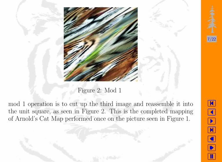
Figure 2: Mod 1

mod 1 operation is to cut up the third image and reassemble it intothe unit square, as seen in Figure 2. This is the completed mappingof Arnold’s Cat Map performed once on the picture seen in Figure 1.

8/22

�

�

�

�

�

�

Order from Chaos?After repeated applications of the cat map, we see some surprising

things happen. The image seems to dissolve into a television-static likestate, and then it inexplicably reforms into the original image! Figure3 shows the effect of repeated applications of the cat map on a 124by 124 pixel image. This may seem quite unusual at first, but it canactually be explained very reasonably. Let us consider the effect ofthe cat map on a single point in the R2 plane of the form (a/n, b/n),where a, b, and n are integers, 0 ≤ a < n and 0 ≤ b < n.

Γ

([a/nb/n

])=

[1 11 2

] [a/nb/n

]mod 1

=

[a+bn

a+2bn

]mod 1

=

[a+bn

mod 1a+2b

nmod 1

]

9/22

�

�

�

�

�

�

Figure 3: The full cycle

10/22

�

�

�

�

�

�

We already know that Γ will map any point in the R2 plane to a pointin the unit square. For a point in the unit square (but not on the upperor right edge) whose x and y coordinates are both rational numberswith lowest common denominator n, Γ will map that point to anotherpoint of the form (c/n, d/n), with 0 ≤ c < n and 0 ≤ d < n. Sincethere are only n2 points of this form, it follows that a point of the form(a/n, b/n) will be mapped back to itself after at most n2 iterations ofthe cat map.

If the unit square has been colored in with a N × N image, wecan consider it to have N 2 points of the form (a/n, b/n) with colorsassigned to them. After each iteration of the cat map to the image, eachcolored point (except for the point (0, 0)) moves to a new position thatwas previously occupied by another colored point. Each point mustreturn to its original position after no more than N 2 iterations of thecat map.

Let us say that if a point returns to its original position after Piterations of the cat map, it has a period of P . We can easily show

11/22

�

�

�

�

�

�

that the period of the point (0, 0) is 1.

Γ

([00

])=

[1 11 2

] [00

]mod 1.

=

[00

]mod 1

=

[0 mod 10 mod 1

]=

[00

]It turns out that the point (0, 0) is the only point with a period of

one. For an N×N image, let the period of each point be represented byPi. The period of the entire picture must then be the lowest commonmultiple of all the Pi. For example, if a picture in the unit squarecontained points with periods of 1, 3, 5, and 15 only, the number ofiterations of the cat map required to return the image to its originalstate would be 15, as in the case of the 124 by 124 pixel image seen inFigure 3.

12/22

�

�

�

�

�

�

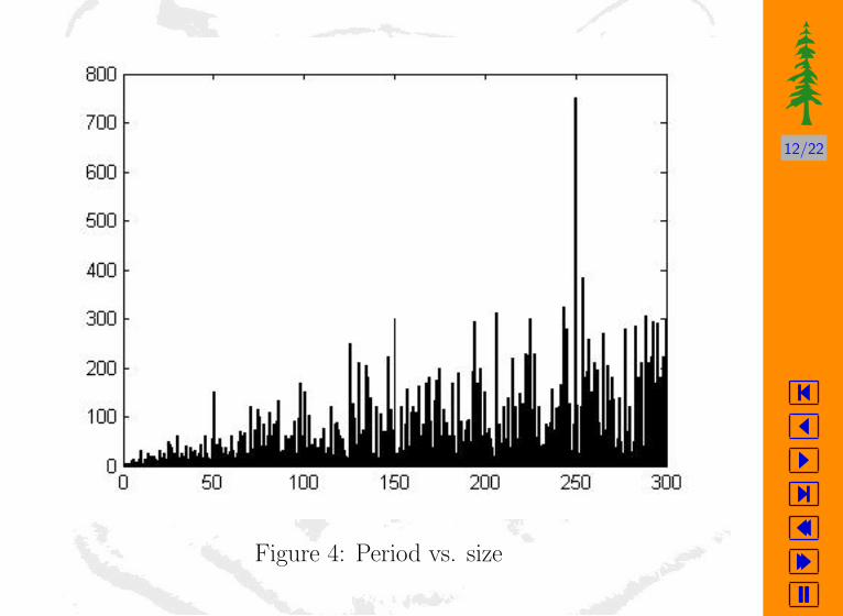
Figure 4: Period vs. size

13/22

�

�

�

�

�

�

Figure 4 shows a graph of the periods of images up to 300 pixels by300 pixels. You can see that the periods vary greatly from one imageto another.

14/22

�

�

�

�

�

�

Streaks and StripesAnother interesting behavior we see following applications of the cat

map is the appearance of diagonal “streaks” in several of the interme-diate images. In order to fully understand why this is happening, wehave to think of the cat map in another way. Because of the mod 1operation, the cat map is not a linear transformation. However, if theentire R2 plane has been “tiled” with an image, and then we transformeach point in the entire plane by multiplying it by the matrix[

1 11 2

]without using the mod 1 operation, we would see the same effect asif we had applied the cat map to just the unit square, with the mod1 operation. We can explain the “streaks” by finding the eigenvectors

15/22

�

�

�

�

�

�

and eigenvalues of the matrix [1 11 2

].

The eigenvalues and corresponding eigenvectors of the matrix[1 11 2

]are

λ1 =3 +√

5

2≈ 2.6180 . . . , v1 =

[1

1+√

52

]≈

[1

1.6180

]and

λ2 =3−

√5

2≈ 0.38196 . . . , v2 =

[1

1−√

52

]≈

[1

−0.6180

].

The “streaks” that appear are in the directions of the two eigenvec-tors of the matrix [

1 11 2

].

16/22

�

�

�

�

�

�

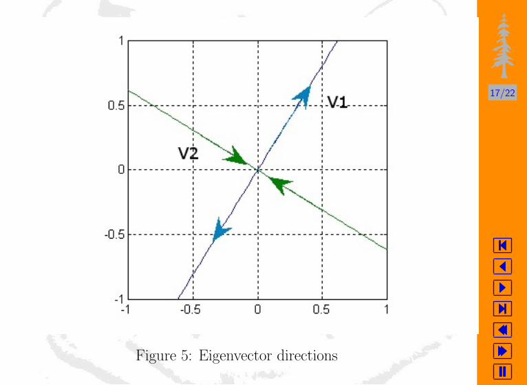
Figure 5 shows the directions of the eigenvectors v1 and v2. As eachvector representing a point in the unit square is multiplied by thematrix [

1 11 2

],

it moves away from its original position in the general direction of thevector [

11.6810

].

Now let us consider a point a in the unit square that is assigneda specific color. If the point a has period P , then somewhere in the“tiled” plane there is another point b that will arrive at the originalposition of point a after the entire plane has been transformed Ptimes. Each time the vector representing the point b is multipliedby the matrix above, it moves closer to the original position of thepoint a, finally arriving there after P multiplications. Upon the finaltransformation of the point b, it moves to the original position of thepoint a in the direction of the eigenvector v2. This is the cause ofthe “streaks” that appear near the end of the cycle, which are in the

17/22

�

�

�

�

�

�

Figure 5: Eigenvector directions

18/22

�

�

�

�

�

�

direction of the eigenvector v2.

19/22

�

�

�

�

�

�

ApparitionsAnother peculiar thing occurs when the cat map is applied to some

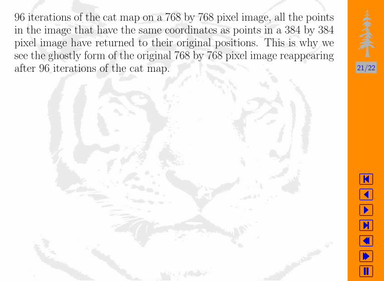
larger images. An image that is 768 pixels by 768 pixels has a periodof 192. Figure 6 shows what happens after 96 iterations of the cat mapon a 768 pixel by 768 pixel image.

In the background of the transformed image we can see a faint,ghostly likeness of the original image. There are also sections of theoriginal image that have been moved to new locations in the trans-formed image. We can explain the appearance of the original imagein the background in the following way. If the unit square has beenpainted with a 768 by 768 pixel image, it consists of colored pointsof the form (i/768, j/768), where i and j are integers, 0 ≤ i < 768and 0 ≤ j < 768. When i and j are multiples of 2, then the pointsreduce to the form (p/384, q/384). These points are the same pointswe would have if we painted the unit square with a 384 by 384 pixelimage. The period of a 384 by 384 pixel image is exactly 96. So after

20/22

�

�

�

�

�

�

Figure 6: The ghost and the darkness

21/22

�

�

�

�

�

�

96 iterations of the cat map on a 768 by 768 pixel image, all the pointsin the image that have the same coordinates as points in a 384 by 384pixel image have returned to their original positions. This is why wesee the ghostly form of the original 768 by 768 pixel image reappearingafter 96 iterations of the cat map.

22/22

�

�

�

�

�

�

References[1] David Arnold, and his extensive knowledge of mathematics, Mat-

lab, Tex, and teaching.

[2] Strang, Gilbert. Introduction To Linear Algebra. 3rd ed. Welles-ley Cambridge Press, 2003.

[3] Anton, Howard, and Rorres Chris. Elementary Linear Algebra.8th ed. New York: John Wiley & Sons, Inc., 2000. 678-688.