Appendix caption

Figure A. 1 Linear regression models between urban land area and urban population under the five SSP scenarios.

Figure A. 2 Parameters used in the LUSD-urban model.

Figure A. 3 Calibrating the LUSD-urban model with the urban expansion simulation in the drylands of northern China from 1992 to 2015.

Figure A. 4 The urban expansion of the drylands of northern China from 2015 to 2050 under SSP2, SSP3, SSP4, and SSP5.

Table A. 1 Basic information on the drylands of northern China.

Table A. 2 The SSP urban population of the drylands of northern China from 1990 to 2050.

Table A. 3 Description of the population and urbanization elements within the SSPs, modified from O’Neill et al. (2014, 2015).

Table A. 4 Weights used in the LUSD-urban model.

1

(a) (b)

SSP1 SSP2(c) (d)

SSP3 SSP4(e)

SSP5

Figure A. 1 Linear regression models between urban land area and urban population under the five SSP scenarios.

2

Figure A. 2 Parameters used in the LUSD-urban model.

3

Figure A. 3 Calibrating the LUSD-urban model with the urban expansion simulation in the drylands of northern China from 1992 to 2015.

(a) Actual urban pattern in 2000, (b) simulated urban pattern in 2000 (Kappa = 0.71), (c) actual urban pattern in 2010, (d) simulated urban pattern in 2010 (Kappa = 0.69), (e) actual urban pattern in 2015, (f) simulated urban pattern in 2015 (Kappa = 0.77).

4

(a) Urban expansion under the SSP2 scenario

5

(a)

(b) Urban expansion under the SSP3 scenario

6

(b)

(c) Urban expansion under the SSP4 scenario

7

(c)

(d) Urban expansion under the SSP5 scenario

Figure A. 4 The urban expansion of the drylands of northern China from 2015 to 2050 under SSP2, SSP3, SSP4, and SSP5.

(a) Urban expansion under the SSP2 scenario,

(b) urban expansion under the SSP3 scenario,

(c) urban expansion under the SSP4 scenario,

(d) urban expansion under the SSP5 scenario.

Note: Please refer to Fig. 1 for the names of cities and urban agglomerations.

8

(d)

Table A. 1 Basic information on the drylands of northern China.

Dryland subtype

Provinces included

in drylands

Area(1000 km2)

Populationin 2010

(million)

GDP in 2010

(billion RMB)

Dry subhumid Inner Mongolia 271.39 3.98 116.82Shanxi 147.74 34.93 890.56Hebei 125.07 65.31 1819.50Heilongjiang 115.56 20.32 738.00Shaanxi 110.19 19.49 521.08Gansu 91.53 8.51 95.49Shandong 83.06 53.56 2144.35Henan 59.38 47.30 1349.64Jilin 45.93 5.43 181.15Beijing 12.20 18.83 1390.44Tianjin 11.55 12.94 922.45Ningxia 2.55 0.20 1.82

Total 1076.13 290.80 10171.30Semiarid Inner Mongolia 347.37 9.63 640.94

Xinjiang 278.85 9.54 276.54Gansu 104.31 13.58 211.65Qinghai 67.91 3.76 83.32Ningxia 49.44 6.10 155.60Heilongjiang 15.10 2.50 55.03Shaanxi 10.02 0.58 43.87Hebei 6.01 0.36 4.90Shanxi 4.99 0.37 8.82

Total 883.98 46.42 1480.65Arid Xinjiang 753.15 9.26 261.08

Gansu 165.06 2.33 351.76Inner Mongolia 450.98 5.18 73.72

Total 1369.18 16.77 686.56Hyper-arid Xinjiang 504.02 2.25 34.99

Qinghai 74.29 0.05 41.01Gansu 42.13 0.20 5.86

Total 620.44 2.49 81.86Drylands 3949.73 356.48 12420.37

9

Table A. 2 The SSP urban population of the drylands of northern China from 1990 to 2050.

YearUrban population (million)

SSP1 SSP2 SSP3 SSP4 SSP51990* 84.79 84.79 84.79 84.79 84.792000* 123.35 123.35 123.35 123.35 123.352005* 146.64 146.64 146.64 146.64 146.642010* 171.05 171.05 171.05 171.05 171.052015** 194.91 188.17 181.74 194.74 194.902020** 218.64 205.05 192.65 218.26 218.602030** 251.96 229.05 206.33 250.19 251.902040** 267.74 240.56 210.67 263.03 267.692050** 267.81 240.38 207.27 258.83 267.81Notes: * Historical urban population from HYDE.** Predicted urban population under different scenarios from HYDE.

10

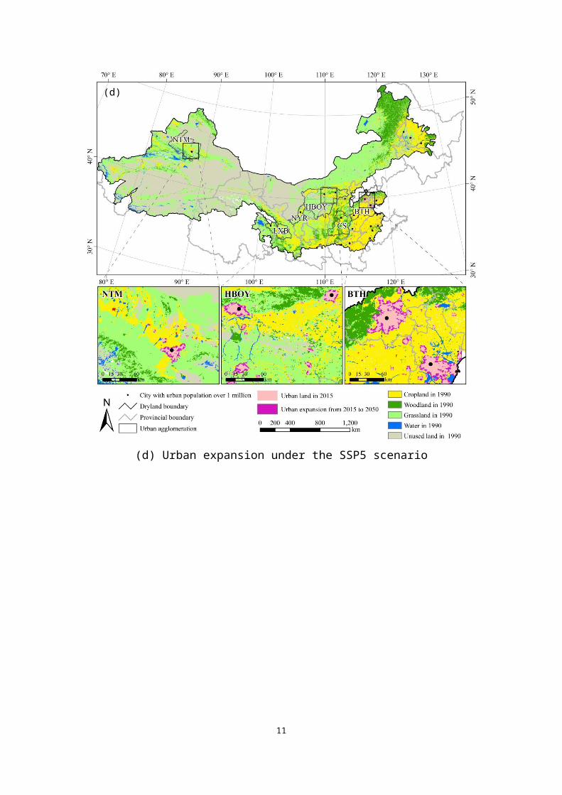
Table A. 3 Description of the population and urbanization elements within the SSPs, modified from O’Neill et al. (2014, 2015).

SSP

SSP 1 SSP 2 SSP 3 SSP 4 SSP 5

Country fertility groupings for demographic elements*

High

fert.*

Low

fert.*

Rich-

OECD**

High

fert.*

Low

fert.*

Rich-

OECD**

High

fert.*

Low

fert.*

Rich-

OECD**

High

fert.*

Low

fert.*

Rich-

OECD**

High

fert.*

Low

fert.*

Rich-

OECD**

Element

Population

Growth Relatively low Medium High Low Relatively high Low Relatively low

Fertility Low Low Medium Medium High High Low High Low Low Low Low High

Mortality Low Medium High HighMediu

mMedium Low

Migration Medium Medium Medium High

UrbanizationLevel High Medium Low High High Medium High

Type Well managedContinuation of

historical patternsPoorly managed Mixed across and within cities

Better management over time,

some sprawl

Challenges Low for mitigation and

adaptationModerate

High for mitigation

and adaptation

High for adaptation, low for

mitigation

High for mitigation, low for

adaptation

Illustrative starting points for

narratives

Sustainable

development proceeds

at a reasonably high

pace, inequalities are

lessened, technological

change is rapid and

directed toward

environmentally

friendly processes,

An intermediate case

between SSP1 and

SSP3.

Unmitigated emissions are

high due to moderate

economic growth, a rapidly

growing population, and slow

technological change in the

energy sector, making

mitigation difficult.

Investments in human capital

are low, inequality is high, a

A mixed world, with relatively

rapid technological

development in low carbon

energy sources in key emitting

regions, leading to relatively

large mitigative capacity in

places where it matters most to

global emissions. However, in

other regions, development

In the absence of climate

policies, energy demand is high,

and most of this demand is met

with carbon-based fuels.

Investments in alternative energy

technologies are low, and there

are few readily available options

for mitigation. Nonetheless,

economic development is

11

including lower carbon

energy sources and high

productivity of land.

regionalized world leads to

reduced trade flows, and

institutional development is

unfavorable, leaving large

numbers of people vulnerable

to climate change and many

parts of the world with low

adaptive capacity.

proceeds slowly, inequality

remains high, and economies

are relatively isolated, leaving

these regions highly

vulnerable to climate change

with limited adaptive capacity.

relatively rapid and is driven by

high investment in human capital.

Improved human capital also

produces a more equitable

distribution of resources, stronger

institutions, and slower

population growth, leading to a

less vulnerable world better able

to adapt to climate impacts.

Note: * See KC and Lutz (2014) for the definitions of country fertility groupings; **OECD: Organization for Economic Co-operation and Development.

12

Table A. 4 Weights used in the LUSD-urban model.

FactorsWeights for simulation1992-2000

2000-2010 2010-2015

Elevation 4 1 5Slope 2 2 2Distance to provincial cities 3 13 4Distance to cities 8 4 11Distance to counties 1 5 1Distance to national roads 5 1 2Distance to provincial roads 1 1 10Distance to highways 1 5 8Distance to railways 7 4 2Distance to high-speed railways 6 7 5Neighborhood effects 32 47 46Inheritance attributes 30 10 4

13