art kang fm v 2.indd mtc 07/25/2008 03:15ampreview.kingborn.net/899000/673355dbdb9b463d97bdef... ·...

ART_Kang_FM v_2.indd MTC 07/25/2008 03:15AM

Radar System Analysis, Design, and Simulation


DISCLAIMER OF WARRANTY

The technical descriptions, procedures, and computer programs in this book have been de-veloped with the greatest of care and they have been useful to the author in a broad range of applications; however, they are provided as is, without warranty of any kind. Artech House, Inc. and the author and editors of the book titled Radar System Analysis, Design, and Simulation make no warranties, expressed or implied, that the equations, programs, and procedures in this book or its associated software are free of error, or are consistent with any particular standard of merchantability, or will meet your requirements for any particular application. They should not be relied upon for solving a problem whose incor-rect solution could result in injury to a person or loss of property. Any use of the programs or procedures in such a manner is at the user’s own risk. The editors, author, and publisher disclaim all liability for direct, incidental, or consequent damages resulting from use of the programs or procedures in this book or the associated software.

For a listing of recent titles in the Artech House Radar Library, turn to the back of this book.


Radar System Analysis, Design, and Simulation

Eyung W. Kang

a r techhouse . com


Library of Congress Cataloging-in-Publication DataA catalog record for this book is available from the U.S. Library of Congress.

British Library Cataloguing in Publication DataA catalog record for this book is available from the British Library.

ISBN-13: 978-1-59693-347-7

© 2008 ARTECH HOUSE, INC.685 Canton StreetNorwood, MA 02062

All rights reserved. Printed and bound in the United States of America. No part of this book may be reproduced or utilized in any form or by any means, electronic or mechanical, including photocopying, recording, or by any information storage and retrieval system, without permission in writing from the publisher.

All terms mentioned in this book that are known to be trademarks or service marks have been appropriately capitalized. Artech House cannot attest to the accuracy of this information. Use of a term in this book should not be regarded as affecting the validity of any trademark or service mark.

10 9 8 7 6 5 4 3 2 1

Disclaimer: This eBook does not include the ancillary media that waspackaged with the original printed version of the book.

�


Contents

Preface xi

Acknowledgments xiii

Introduction xv

ChApteR 1 Matrix,Vector,andLinearEquations 1

1.1 Introduction 11.2 Simultaneous Linear Equation 1

1.2.1 Gaussian Elimination with Backsubstitution 21.2.2 Gaussian Elimination with Forward Substitution 4

1.3 Matrix Factorization 51.3.1 LU Factorization 51.3.2 LLT Factorization (Cholesky) 71.3.3 LDLT Factorization (Modified Cholesky) 81.3.4 UDUT Factorization 101.3.5 QR Factorization 11

1.4 Matrix Inversion 151.4.1 L-1

1 161.4.2 L-1

x 171.4.3 U-1

1 191.4.4 U-1

x 201.4.5 D-1 211.4.6 Q-1 21

1.5 Vector Operations 211.6 Matrix Operations 221.7 Conclusion 23

Selected Bibliography 24

ChApteR 2 PseudorandomNumber,Noise,andClutterGeneration 25

2.1 Introduction 252.2 Pseudorandom Numbers and Unit Uniform Variables 25

2.2.1 PRN Generation of an Arbirary Population 272.3 White Gaussian Noise 282.4 Rayleigh Noise 302.5 Rician Random Variables, Signal-to-Noise Ratio 312.6 Chi-Squared Noise 35

�i Contents


2.7 Square-Law Detector 362.8 Exponential Noise 382.9 Lognormal Clutter 40

2.10 Weibull Clutter 422.11 Postulate of Probability Density Function from Sampled Data 442.12 Construction of Gaussian (Normal) Probability Paper 492.13 Conclusion 51

References 52

ChApteR 3

Filters,FIR,andIIR 53

3.1 Introduction 533.2 Finite Impulse Response Filter (FIR) 56

3.2.1 FIR Filters: Lowpass, Highpass, Bandpass, and Bandstop 563.2.2 Window Functions: Rectangle, von Hann, Hamming, and

Blackman 593.2.3 Kaiser Filter: Lowpass, Highpass, Bandpass, and Bandstop 65

3.3 Infinite Impulse Response Filter (IIR) 683.3.1 Bilinear Transform 693.3.2 Review of Analog Filters 713.3.3 IIR Filter, Butterworth Lowpass 833.3.4 IIR Filter, Chebyshev Lowpass 843.3.5 IIR Filter, Elliptic Lowpass 853.3.6 IIR Filter, Elliptic Bandpass 873.3.7 Issue of Nonlinearity 893.3.8 Comparison Between FIR and IIR Filters 903.3.9 Quantized Noise and Dynamic Range of A/D Converter 90References 94

ChApteR 4 FastFourierTransform(FFT)andIFFT 95

4.1 Introduction 954.2 Fast Fourier Transform Decimation-in-Time and Decimation-

in-Frequency 964.3 Demonstration of FFT_DIT and FFT_DIF 1014.4 Spectral Leakage and Window Function 1044.5 Inverse Fast Fourier Transform Decimation-in-Time, and Decimation-

in-Frequency 1064.6 Applications of FFT and IFFT 107

4.6.1 Filtering in the Frequency Domain 1094.6.2 Detection of Signal Buried in Noise 1104.6.3 Interpolation of Data 1104.6.4 Pulse Compression 1104.6.5 Amplitude Unbalance and Phase Mismatch 118Appendix 4A 122References 124

Contents �ii


ChApteR 5 AmbiguityFunction 125

5.1 Introduction 1255.2 Rectangle Pulse with a Single Constant Frequency 1265.3 Linear Frequency Modulation (LFM) 1285.4 Costas-Coded Frequency Hopping Modulation 131

References 140Selected Bibliography 141Appendix 5A 141

ChApteR 6 ArrayAntennas 143

6.1 Introduction 1436.2 Linear Array 1436.3 Circular Aperture Array 1496.4 Elliptical Aperture Array 1536.5 Monopulse Aperture Array 1546.6 Conclusion 159

References 161Appendix 6A 162Closing Remarks 163

ChApteR 7 TargetDetection 165

7.1 Introduction 1657.2 The Probability of Detection and the False Alarm

Probability for Marcum’s Target Model 1697.3 The Probability of Detection, Swerling Target Models 180

7.3.1 Swerling Target Model 1 1837.3.2 Swerling Target Model 2 1867.3.3 Swerling Target Model 3 1877.3.4 Swerling Target Model 4 190

7.4 Conclusion 192References 196Selected Bibliography 197

ChApteR 8 KalmanFilter 199

8.1 Introduction 1998.2 Derivation of Kalman Filter Equations 2028.3 Passenger Airliner 2118.4 Air Traffic Control Radar 2148.5 Air Defense Radar, Cartesian Coordinate System 223

�iii Contents


8.6 Air Defense Radar, LOS Coordinates 2338.7 Kalman Filter without Matrix Inversion 238

References 245Selected Bibliography 246

ChApteR 9 MonteCarloMethodandFunctionIntegration 247

9.1 Introduction 2479.2 Hit-or-Miss Method 2479.3 Ordered Sample Method 2519.4 Sample Mean Method 2529.5 Importance Sampling Method 2539.6 Observations and Remarks 2559.7 Probability of False Alarm, Exponential Probability Density Function 2569.8 Probability of False Alarm, Gaussian Density Function 2609.9 Integration of Functions 265

9.9.1 Trapezoidal Rule 2659.9.2 Simpson’s Rule and Extended Simpson’s Rule 2669.9.3 Gaussian Quadrature 267

9.10 Quadrature in Two Dimensions 2759.11 Quadrature in Three Dimensions 2789.12 Concluding Remarks 279

References 280Appendix 9A 280

ChApteR 10 ConstantFalseAlarmRate(CFAR)Processing 281

10.1 Introduction 28110.2 Cell Average CFAR (CA-CFAR) 28110.3 Order-Statistics CFAR (OS-CFAR) 28910.4 Weibull Clutter 295

10.4.1 Weibull Probability Density Function 29510.4.2 Weibull Clutter After a Square-Law Detector 297

10.5 Weber-Haykin CFAR (WH-CFAR) 29910.6 Maximum Likelihood CFAR (ML-CFAR) 30510.7 Minimum Mean Square Error CFAR (MMSE-CFAR) 31310.8 Conclusion 319

References 320Selected Bibliography 321

Contents ix


ChApteR 11 MovingTargetIndicator 323

11.1 Introduction 32311.2 Nonrecursive Delay-Line Canceller 32311.3 Recursive Delay-Line Canceller 32711.4 Blind Speed and Staggered PRFs 33111.5 Clutter Attenuation and Improvement Factor 33411.6 Limitation Due to System Instability 34611.7 A/D Converter Quantization Noise 34811.8 Clutter Map 34911.9 Conclusion 349

References 350

ChApteR 12 MiscellaneousProgramRoutines 351

Index 355

xi


Preface

This book aims to reach radar system engineers who strive to optimize system per-formance and graduate students who wish to learn radar system design. It addresses the need to master system analysis and design skills and to verify that the analysis is correct and that the design is optimal through simulation on a digital computer. The prerequisites for understanding most of topics in this book are rather minimal: an elementary knowledge of probability theory and algebraic matrix operations and a basic familiarity with the computer.

Achieving the right balance between the depth and breadth of each chapter subject has been a difficult task. Readers may recognize that full coverage of each chapter title could fill its own a separate book of substantial volume. An attractive feature of this book is that it allows readers to build a solid foundation and increase their level of sophistication as their experience grows.

This book is intended for those readers who have an impatient urge to learn radar system analysis and design and C++ programming with applications. All exam-ples are explained in detail in the text, and the numerical results are either displayed on screen or stored in .DAT files and shown in graphic form when appropriate. This book is not C++ for dummies; this book is for smart students and diligent engineers who are overloaded with other burdens.

So let’s get started! The mountaintop is not that far away, and the path to be traversed to reach the top is not too arduous a climb.

xiii


Acknowledgments

This introductory book will help readers to build a solid foundation for further explorations in their chosen topics.

Many friends and colleagues helped me and encouraged me to complete the manuscript. I owe them a large debt of gratitude. I wish I could acknowledge them all by name, but they are too numerous.

I am most grateful to Mrs. Mary K. Darcy who patiently taught me how to type the mathematic equations clearly and concisely. Her indefatigable tutoring in presenting the graphs and diagrams made this book stand apart from all others with a similar title.

x�


Introduction

Chapter 1: Matrix, Vector, and Linear equations

Chapter 1 introduces matrix-vector operations. We start with how to solve a set of simultaneous linear equations by Gauss’s elimination methods of the back-substitution and forward substitution that we learned in earlier years in school. When the dimen-sion of equations is two or three we can solve for the unknowns with pencil and paper. When the dimension is higher than, say, four or higher we would rather resort to a computer program.

We encounter immediately the task of matrix inversion. Matrix inversion is usu-ally permissible, but sometime it is not, depending upon the structure of the matrix. We learn when it is permissible by means of matrix factorization (decomposition). The factored matrices would clearly indicate whether the inversion is permissible. Several popular factorization routines and the corresponding inversions of factored matrices are programmed.

Vector operation is treated as a subset of matrix operations. Two header files, VECTOR.H and MATRIX.H, are constructed in order to determine when the matrix-vector operations are called for in the main driver.

Chapter 2: pseudorandom Number (pRN), Noise, and Clutter Generation

The goal of this chapter is to generate various noises and clutters we would encoun-ter in signal processing. The noise and clutter are characterized by the probability density function and its mean and variance. (For those who prefer electrical terms mean is DC voltage level and variance is AC power.) The basic building components of noise and clutter are unit uniform random variables, and the unit uniform vari-ables are, in turn, generated from pseudo-random numbers (PRNs). There are a few prepackaged random number generators; however, careless use of these generators causes some intractable confusion in the results of signal processing.

We start with PRN generation by mixed congruential method. This method generates a random number vector without missing data nor duplicated data in a specified population N after a correction. It is contiguous in the given range. Some of the off-the-shelf packages seldom meet the requirement of contiguity.

The typical noise and clutter we encounter most often in signal processing, such as Gaussian, Rayleigh, Rician, exponential, and chi-squared, and lognormal, Weibull clutters, are generated. The computation of noise power or clutter power is empha-sized. These noises or clutters are used in applications programs in such areas as filter design, pulse compression, Kalman filters, and the Monte Carlo technique.


Chapter 3: Filters, FIR, and IIR

In this chapter we program filter designs. Filters are broadly classified into two groups: finite duration impulse response filters, and infinite duration impulse re-sponse filters. The word duration is deleted, and we call them the finite impulse response (FIR) filters, or infinite impulse response (IIR) filters for short.

The design of a FIR filter is based on the inverse Fourier transform of the im-pulse response of lowpass, highpass, bandpass, and bandstop. The structure of the FIR filter is nonrecursive, and the phase response is a linear function of frequency. The design of the IIR filter is based on the analog filter designs abundantly avail-able in textbooks and tables. The analog frequency response is transformed to the z-domain using bilinear transform and prewarping the response. The structure is recursive, and the phase versus frequency is nonlinear.

Several window functions (the envelope functions) to control the level of side-lobes are described in detail and incorporated in the design, and the advantages and disadvantages of FIR and IIR are discussed.

Chapter 4: Fast Fourier transform (FFt) and IFFt

The real-time processing of Fourier transforms became possible when the fast Fou-rier transform algorithm was discovered in the early 1960s. Prior to this discovery the “real-time on-line” computation of frequency content had been impractical.

The fast Fourier transform is implemented either by decimation-in-time (DIT) or decimation-in-frequency (DIF) algorithm, with a suitable bit-reversal operation. The proper sequence of the bit-reverse operation is shown in a block diagram to show the proper order of bit-reversal in DIT and DIF.

An improper sampling of signals would produce spectral leakage and unfaithful reproduction of time function. A detailed discussion to remedy these problems are given, and examples are shown.

Applications of the fast Fourier transform and inverse transform in signal pro-cessing are numerous and include determining how to extract a signal buried in noise, how to compress a frequency-modulated pulse to improve resolution, and how to correct an unbalanced and mismatched I/Q channels of a coherent receiver. We present a few of these interesting applications.

A clear explanation together with a system block diagram will help readers to understand the concept involved. The results of programs are stored in .DAT files, and the corresponding graphs are shown.

Chapter 5: Ambiguity Function

This chapter is written for those who would like to explore the pulse compression in depth. We start with a rectangular pulse with constant carrier frequency and learn basic characteristics of a simple pulsed signal.

x�i Introduction


A popular signal for pulse compression is a coherent linear frequency-modulated (CLFM) pulse. Most high-performance radar systems have adopted the CLFM pulse, and the returned signal is compressed via FFT and IFFT algorithms in real time.

Analysis of the ambiguity function has indicated that there are many more modulation schemes to increase compression gain, to reduce sidelobe level, to im-prove resolution, and to maintain the low probability of intercept.

One ideal modulated pulse is the Costas-coded frequency-hopping modula-tion. We have programmed the Costas-coded signal and concluded that the Cos-tas-coded signal is very nearly an ideal pulse. The correct sequence of frequency hopping is analyzed, and the result is presented in an ambiguity surface in three dimensions.

Chapter 6: Array Antennas

This chapter presents the array antenna design. A simple line array antenna is ana-lyzed and programmed. A circular or elliptical array design is an extension of a line array design. The amplitude distributions of array elements are controlled by window functions such as Hamming, Chebyshev, Taylor, and Lambda. The maxi-mum gain, 3-dB beamwidth, and the sidelobe levels are compared with a rectangle window. A similarity between the window functions in filter design is mentioned. A monopulse array antenna, an essential component of a tracking radar system, is followed.

Elimination (or cancelation) of mutual reactance coupling among array ele-ments is excluded from the discussion, for the coupling is entirely dependent upon the physical structure of the element of radiation source and the geometric distribu-tion of elements on the array aperture.

This chapter does not cover the intricacies and difficulties in designing and manufacturing an array antenna. However, it provides, under an ideal condition, what we expect of the maximum gain, the beamwidth, and the sidelobe levels when the dimension of the array aperture and window function are specified. The refer-ences are cited for those problems we have not addressed.

Chapter 7: target Detection

This chapter presents the theory of the probability of detection and the probability of false alarm. The detection probability and the false alarm probability are intro-duced heuristically at the beginning in order to put readers at ease.

The detection processing involved in the heuristic model is shown in a recircu-lating accumulator. The relationship between the detection probability Pd, the false alarm probability Pfa and the threshold level Vth is programmed and discussed. The threshold level Vth (or bias level yb) is a function of the number of pulse N to be accumulated (summed) in the recirculator-accumulator; the larger the number of pulses the lower the Vth (or yb) for a specified Pfa.

Introduction x�ii


The mathematic expression for Pfa is formally derived as a function of the bias level yb. An expression of Pd is derived, in turn, as a function of both the number of pulses N and the signal-to-noise ratio S/N (in power) per pulse.

Four factors, Pd, Pfa, N, and S/N, maintain an interlocked relationship; that is, if we specify any combination of three factors, the fourth will be determined uniquely. One remaining problem is how to characterize the target signals. The retuned sig-nals are grouped into five Marcum’s and Swerling’s targets in honor of the pioneer investigators.

Marcum’s target is nonfluctuating, a constant cross-section target, like a large metallic sphere of several wavelengths in diameter. A large spherical target reflects a constant power irrespective of the aspect angle of the antenna beam. Two programs are written for Marcum’s target, and the results are shown in a table as well as in the following graphic forms:

· Pd_(0)_1.CPP Detection probability, Marcum’s target, N =1· Pd_(0)_N.CPP Detection probability, Marcum’s target, N³2

Swerling has grouped the fluctuating targets in four different types: target model 1, 2, 3, and 4.

The probability density function of the target cross-section is assumed to be Rayleigh-distributed for target models 1 and 2, and the rate of fluctuation is either slow or rapid. Rayleigh-slow is Swerling’s target 1, and Rayleigh-rapid is Swerling target 2.

The target cross-section of Swerling’s 3 and 4 is assumed to be distributed chi-squared with four degrees of freedom, and the fluctuation is either slow or rapid. Slow or rapid fluctuation is a relative term with respect to the dynamics of target and the radar operation parameters such as transmitting frequency, the pulse repeti-tion frequency (fPRF), and the antenna rotation rate.

Eight programs are written for Swerling’s targets. The false alarm probability is set at 1.0E-6, adjustable to 1.0E-5. The detection probability is computed as a func-tion of S/N per pulse with the number of pulse N integrable as a variable parameter. The eight programs are listed as follows:

· Pd_(l)_1.CPP: Swerling target 1, N=1;· Pd_(l)_N.CPP: Swerling target 1, N=2, 4, 8, 16, . . . ;· Pd_(2)_1.CPP: Swerling target 2, N=1;· Pd_(2)_N.CPP: Swerling target 2, N=2, 4, 8, 16, . . . ;· Pd_(3)_1.CPP: Swerling target 3, N=1;· Pd_(3)_N.CPP: Swerling target 3, N=2, 4, 8, 16, . . . ;· Pd_(4)_1.CPP: Swerling target 4, N=1;· Pd_(4)_N.CPP: Swerling target 4, N=2, 4, 8, 16, . . . .

The noise is for all programs Gaussian with zero mean and unity variance, which transformed to exponential after a square-law detector as presented in Chapter 2.

An example of a preliminary system design is given at the end. For instance, when we specify the transmitter frequency and power, the antenna gain, the hardware

x�iii Introduction


plumbing loss the RF section and the noise figure, the predetection bandwidth of the receiver, the number of pulses N integrable, at what distance might we be able to de-tect a target of 10m2 with a detection probability of 90% (or 50%) if the target is a nonfluctuating Marcum’s target? We answer this question clearly. The detection range for the fluctuating Swerling’s targets can be deduced from the programs given above.

The detection probability when the Gaussian noise is replaced by clutter returns is separately analyzed and programmed in Chapter 10, since the detection prob-ability under clutter intrusion requires an additional theoretical development and processing implementation.

Chapter 8: Kalman Filter

We define the symbols and notations used in this chapter at the outset. This is to eliminate the confusion and frustration that might stem from reading a few text-books and research papers by various authors.

The bold letters represent vectors or matrices. Some vectors and matrices have an overhead symbol, a caret (^) or a tilde (~). The caret signifies that the vector or matrix is an estimate. The tilde, on the other hand, signifies the difference between an estimate and the true state. In addition, the vector and matrix have subscript k-1, k, or k+1. The k-1 connotes the vector or matrix is a state of immediate past, the k the present. The k+1 is a predicted state, one sample time in the future. The vector or matrix without a subscript is time-invariant, and the vector or matrix without an overhead symbol is the true state, unknowable to the observer.

Example 1We derive seven equations of Kalman filter through an example. A simple example of Kalman filter processing is a radar system that tracks a passenger airliner whose flight trajectory is a straight line at a constant altitude without any abrupt maneuver. We assume that the airliner experiences a small random deviation from an ideal straight line due to atmospheric disturbance and nonuniform engine thrust. We define the state equation of the airliner and the measurement (observation) equation by a ra-dar. The atmospheric disturbance and nonuniform thrust are assumed to be small in magnitude, and the probability distribution is Gaussian. Two sources of measurement errors are due to finite transmitter pulsewidth (range error) and finite antenna beam-width (azimuth error). The probability density function of the measurement errors is a unit uniform; that is, the error is most likely distributed equally and uniformly. Numerical examples are given whenever a new vector or matrix is introduced.

Three programs are written: an equation of a straight-line trajectory in x-y co-ordinates; a Gaussian deviation of zero mean and variance of 0.5g, which is added to the straight line to simulate the actual flight path; and the measurement equation by the radar. The estimated and predicted error covariance matrices P+

k and P–k+1 are

derived as well as the Kalman gain matrix kk. The estimated state and predicted state, x+

k and x–k+1 (the position of airliner) are derived, with the Kalman gain matrix kk as

an input.

Introduction xix


The filter processing is shown in a flow diagram. The filter has two recursive loops; one computes the estimated and predicted error covariance matrices, and the other loop computes the estimated and predicted states. The two loops are con-nected by a Kalman gain matrix.

A post-flight analysis is programmed to evaluate the performance of the Kal-man filter. The error between the true trajectory and the estimated and the predicted positions of the airliner are presented for discussion. An improved initialization of the error covariance matrix and that of the state vector are discussed.

Example 2The second example is air traffic control (ATC) radar. There are two types of ATC radars: airport surveillance radar (ASR) and air route surveillance radar (ARSR). The former is for a short range, the latter for a longer range. An ASR system with a Kalman tracking filter is programmed in the line-of-sight (LOS) coordinates while an airliner approaches an airport.

The transmitter pulsewidth (0.83 µs) and the antenna beamwidth (1.5 degrees), the sources of range measurement error, and the azimuth error are incorporated in the numerical example to demonstrate how a practical Kalman filter really works.

The elements of estimated and predicted error covariance matrices are in terms of LOS coordinates, as are the estimated and predicted airliner’s state. A post-flight error analysis is programmed, and the results are presented in graphic form. The advantages and disadvantages of formulating the filter in LOS coordinates system are discussed.

Example 3 and 4The third and fourth examples are that of a short-range ground-based air defense radar; one operates in the LOS coordinates and the other in the Cartesian coordi-nates system (CCS). The target is a fighter-bomber on a ground-attack mission with a “turn-dive-attack and turn-climb-escape” maneuver with a maximum accelera-tion of ± 3g. The random acceleration noise matrix Qk and the measurement error matrix Rk are derived, and the coordinate transformation between LOS and CCS is given. The initialization of the estimate of the error covariance matrix Pk(k=2) instead of Pk(k=0) is discussed in detail.

The tracking performances in the LOS and CCS systems are presented for com-parison. The recursive processing sequences are shown in a block diagram.

Example 5The fifth example emphasizes the problems associated with a matrix inversion, and a Kalman filter without a matrix inversion is presented. We note the special characteristic of the error covariance matrix Pk; it is always symmetric and positive definite. The covariance matrix is factored (decomposed), and we recognize that an inversion is equivalent to a scalar division after factorization.

The Kalman filter without a matrix inversion is programmed. The target is identi-cal to example 3 or 4. The result shows that the difference between “with inversion” and “without inversion” is practically nil. The computation load of no-inversion is, however, slightly higher.

xx Introduction


A block diagram of “no-matrix-inversion” is given. The basic processing se-quences are not altered; they are two recursive loops, one for the error covariance matrices and the other for state vectors, connected by Kalman gain matrix.

Chapter 9: Monte Carlo Method and Function Integration

In this chapter we learn the basic principles of the Monte Carlo method through examples. We begin with the most simple technique of the “hit-or-miss” method. From this method we learn that the number of sampled data must be on the order of tens of thousands or more to obtain an acceptable level of precision.

The hit-or-miss method is followed by the “ordered sample method” and the “sample mean method” to reduce the number of replications. We present the subject of the coefficient of dispersion (CD) to determine the replication number required for a desired level of precision. The last method we study is the “impor-tance sampling method,” a most popular technique among researchers in the field. Mathematics involved in the importance sampling are derived in detail, and two examples are given.

This chapter concludes with several function integration routines found in the elementary calculus books, since the Monte Carlo technique is a numerical experi-mental mathematic process of integration and a probabilistic determination of a rare event occurrence out of a large number of trials.

Chapter 10: Constant False Alarm Rate (CFAR) processing

Equations are derived to show the interlocking relationship among the probability of detection, the probability of false alarm, the threshold level, and the number of samples stored in the reference window.

We entertain a scenario of radar in surveillance mode when an antenna sweeps from one sector to another. The antenna will receive different noise or clutter power locally varying. The threshold (or bias level) must be adjusted automatically to maintain the false alarm at a constant level. In this chapter we derive mathematic equations for the threshold when statistically stationary and uniformly distributed noise or clutter is encountered. The crux of the solution is an accurate estimate of the noise or clutter power.

Example 1: CA-CFARWe present the “cell-average” technique in estimating the noise power in detail. The noise is assumed to be Gaussian-distributed with zero mean and unknown vari-ance. CA-CFAR processing is simple in concept and easy to implement; however, it has a sluggish response to a rapid change in noise level. The CA-CFAR incurs a processing loss inversely proportional to the number of reference cells employed in estimating the noise power. The loss in decibels as a function of the number of refer-ence cells is derived. The most detrimental to a successful operation is the absence

Introduction xxi


of an adequate means to deal with multiple targets in the reference cells, since these spurious targets would raise the threshold erroneously higher.

Example 2: OS-CFARWe investigate a CFAR technique with a censoring mechanism, called “order-statistics” (OS) processing, or OS-CFAR for short, to handle the multiple-target situation. The received noise data stored in the reference window is rank-ordered (rearranged) by increasing order of magnitude, and we censor (discard) one, two, three, or four of the highest data in estimating the noise power. The underlying principle comes from the theory of order statistics. The distribution of noise after the censor has been known to us. We have applied the theory to the problem.

We have derived the equations of the false alarm probability, the threshold multiplication factor T, and the signal-to-noise (S/N) ratio (in power) per pulse. The results indicate that OS-CFAR has eliminated the problem of multiple targets in the reference window with a small fraction of additional processing loss. We also found that the response to a sudden change in noise level is faster than that of CA-CFAR. The OS-CFAR offers the most robust processing, provided that the noise (or clutter) is Gaussian-distributed, variance-unknown.

CFAR processing in clutter. The reflected power from the land and sea are re-ported to be more likely distributed as log-normal or Weibull rather than a benign Gaussian. The log-normal distribution is characterized by tall spiky waveforms. The probability density function has the longest tail.

The Weibull is a two-parameter distribution: the shape parameter c and the scale parameter b. Depending on the shape parameter, the Weibull probability den-sity function may be an exponential, or Rayleigh, or a Gaussian look-alike with a small skew to the right. Weibull is a versatile function to characterize the clutter returns that vary spatially or temporally.

We study some statistics of Weibull distribution (i.e., mean, variance, moments, me-dian, mode, and quantiles). Weibull clutters that pass through a square-law detector re-main Weibulls, though the shape parameter is halved and the scale parameter is squared. We take advantage of this unique transformation of Weibull in CFAR processing.

Example 3: Weber-Haykin CFAR, WH-CFARWeber and Haykin proposed CFAR processing in Weibull clutter. We follow their analysis and present a few numerical results, since they have not provided any. The task is to estimate the two parameters simultaneously from the clutter returns stored in the reference window. The false alarm probability and the threshold are programmed. We present two results with uncensored and censored algorithms. The processing losses are compared with CA-CFAR and OS-CFAR, and we found that WH-CFAR exacts a very high loss in Weibull clutter.

Example 4: Maximum Likelihood CFAR, ML-CFARThe principle of maximum likelihood estimation is applied to CFAR processing. Mathematic expressions for an estimate of the shape parameter and the scale pa-rameter are given. An estimate of the shape parameter can only be obtained through

xxii Introduction


an iterative procedure since the expression is in a transcendental form. An estimate of scale parameter is obtained by using the iteratively estimated shape parameter.

The shortcoming of the maximum likelihood estimate of the shape parameter is a large biased result when the number of sampled data (the stored clutter samples in the reference window) is relatively small (i.e., 8, 16, or 32).

The biased estimate must be corrected before computing the scale parameter.The bias is negligible when the samples are larger than 100. (We rarely have a

window length of 100.) We have programmed ML-CFAR without a censor and found that the loss is less than that of WH-CFAR; however, it is doubtful that real-time on-line implementation due to the computation burden imposed by the iterative procedure.

Example 5: Minimum Mean Square Error CFAR, MMSE-CFARTo avoid the laborious iterations in ML-CFAR we apply the minimum mean square error analysis to estimate the shape and scale parameter of Weibull-distributed clut-ters. The received clutter data stored in the reference window are rank-ordered (re-arranged) in ascending order of magnitude. The rank-ordered clutter samples in a natural logarithm is a linear function of the parameters with small deviations from a straight line. A regressive straight line with the minimum mean squared error discloses two parameters; the slope of the straight line is an estimate of the shape parameter, the intercept point an estimate of the scale parameter. The computations involved are simple enough for a real-time implementation.

Chapter 11: Moving target Indicator (MtI)

A moving target indicator (MTI) is one of perhaps half a dozen indispensable signal processing methods for the successful operation of a surveillance or tracking radar. A MTI is designed on the principle of Doppler frequency detection (the phase dif-ferential with respect to time). All moving objects produce Doppler frequency pro-portional to the relative velocity of the target and the observer.

We present the implementations of recursive and nonrecursive delay line can-celers of various orders and discuss their performance. We mention the origin of blind speed and design approaches to mitigate it by staggering the pulse repetition frequency, fPRF. An example of ATC radar is given for stagger management.

The definition of clutter attenuation (CA) and the improvement factor (I) in decibels is given to evaluate the performance of various MTI filters. The clutter at-tenuation and the improvement factor would deteriorate when the clutter distribu-tion has a nonzero mean velocity and a broader variance. The system instabilities also cause deterioration. Two examples are given.

Chapter 12: Miscellaneous program Routines

This chapter has collected two scores of C++ programs that do not fit with the chapter title or with the program routines in preliminary preparation for the main program. I hope that readers will benefit from the collections in this chapter.

Introduction xxiii

�

ART_Kang_Ch01 v_2.indd Achorn International 07/25/2008 03:23AM

�

C h a p t e r 1

Matrix, Vector, and Linear Equations

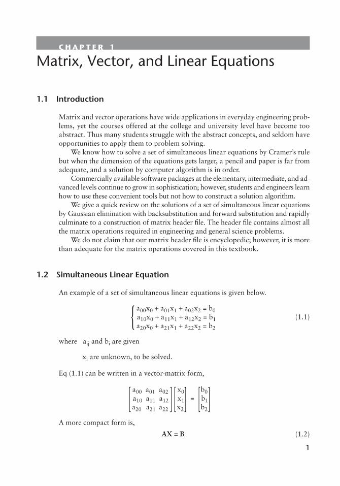
1.1 Introduction

Matrix and vector operations have wide applications in everyday engineering prob-lems, yet the courses offered at the college and university level have become too abstract. Thus many students struggle with the abstract concepts, and seldom have opportunities to apply them to problem solving.

We know how to solve a set of simultaneous linear equations by Cramer’s rule but when the dimension of the equations gets larger, a pencil and paper is far from adequate, and a solution by computer algorithm is in order.

Commercially available software packages at the elementary, intermediate, and ad-vanced levels continue to grow in sophistication; however, students and engineers learn how to use these convenient tools but not how to construct a solution algorithm.

We give a quick review on the solutions of a set of simultaneous linear equations by Gaussian elimination with backsubstitution and forward substitution and rapidly culminate to a construction of matrix header file. The header file contains almost all the matrix operations required in engineering and general science problems.

We do not claim that our matrix header file is encyclopedic; however, it is more than adequate for the matrix operations covered in this textbook.

1.2 Simultaneous Linear Equation

An example of a set of simultaneous linear equations is given below.

a00x0 + a01x1 + a02x2 = b0 { a10x0 + a11x1 + a12x2 = b1 (1.1) a20x0 + a21x1 + a22x2 = b2

where aij and bi are given

xi are unknown, to be solved.

Eq (1.1) can be written in a vector-matrix form,

a00 a01 a02 x0 b0 [ a10 a11 a12 ] [ x1] = [ b1] a20 a21 a22 x2 b2

A more compact form is,

AX=B (1.2)

� Matrix, Vector, and Linear Equations


We want to solve for the column vector Xgiven a matrix A and a column vector B. There are two ways to solve for X;one is using Cramer’s rule and the other by the elimination technique. When the dimension of A is fairly large the determinant and cofactors required for Cramer’s rule become very involved and tedious. The elimination technique is deceptively simple and straightforward.

Before we study the elimination technique we have to delve into the so-called consistency of (1.2). An illustration shows what we mean by consistency.

Consider the following simultaneous equations.

{ x1 + x2 = 5 2x1 + 2x2 = 11

Obviously if one is true the other cannot be, since the second equation is incom-patible or inconsistent with the first one. The inconsistency is visually apparent in this simple case. Consider the following simultaneous equations. A visual inspec-tion for consistency is difficult if not impossible.

2x0 + 3x1 + x2 = 14 [1] { x0 + x1 + x2 = 6 [2] (1.3) 3x0 + 5x1 + x2 = 10 [3]

When we do the following operation, we find that 0 = 12.

2·[1] - {[2]+[3]}

Equation (1.3) is inconsistent; therefore, we do not have a solution for vector X.Imagine that the dimension of A is larger than, say ten! The test of consistency

involves the rank test on matrix A. Numerous good textbooks spend multiple pages on the definition, theorem, and proof of the rank test. Beginners would im-mediately loose interest, become discouraged, and abandon the matrix theory—a tragic loss.

We dispense with a lengthy dissertation on the rank test. Instead we recommend a test on the determinant of A for consistency. If the determinant is nonzero, the simultaneous equations are consistent. Readers may protest that the computation of the determinant is as difficult as the rank test. We therefore strive for a method of computation of the determinant as simple as practicable through matrix factoriza-tion and simpler inversion of the factorized (decomposed) matrices. First we study how to solve simultaneous linear equations by the elimination technique.

1.2.1 Gaussian Elimination with Backsubstitution

We plan to solve the following simultaneous linear equations by backsubstitution. The consistency test is, for the moment, assumed to be satisfied.

2x0 + x1 + 3x2 = 11 [1] { 4x0 + 3x1 + 10x2 = 28 [2] (1.4) 2x0 + 4x1 + 17x2 = 31 [3]


The following table describes the steps taken for back-substitution.

Step taken a0 a1 a2 bi [eq]

2 1 3 11 [1] 4 3 10 28 [2]

2 4 17 31 [3]

[1] 2 1 3 11 [4] [2] – 2[1] 0 1 4 6 [5] [3] − [1] 0 3 14 20 [6]

[4] 2 1 3 11 [7] [5] 0 1 4 6 [8] [6] − 3[5] 0 0 2 2 [9]

When we write equations [7]–[9] appear as follows:

2x0 +x1 + 3x2 = 11 [7] x1 + 4x2 = 6 [8] 2x2 = 2 [9]

From equation [9] we obtain x2=1. The result is substituted into equation [8], and we obtain x1=2. The results are again substituted into equation [7], and we obtain x0=3. The substitution is always backward: x2 first, x1 next, and x0 last. We note that the original square matrix A is transformed to an upper triangle matrix U, and the column vector B is altered.

⎡⎣

a00 a01 a02a10 a11 a12a20 a21 a22

⎤⎦

⎡⎣

x0x1x2

⎤⎦=

⎡⎣

b0b1b2

⎤⎦ →

⎡⎣

a00 a01 a02a �

11 a �12

a ��22

⎤⎦

⎡⎣

x0x1x2

⎤⎦=

⎡⎣

b0

b�1

b��2

⎤⎦

A simple deduction gives the elements of an upper triangle matrix U in terms of the original matrix A: finding the relationship between the primed elements in U in terms of the elements in A. (The first row of A and the first element of B are unchanged). The conversion of A to U is given by,

(intermediate steps)

⎧⎪⎨⎪⎩

a�11 = a11 − (a10/a00)a01

a�12 = a12 − (a10/a00)a02

b�1 = b1 − (a10/a00)b0

⎧⎪⎨⎪⎩

a�21 = a21 − (a20/a00)a01

a�22 = a22 − (a20/a00)a22

b�2 = b2 − (a20/a00)b0

�a��22 = a�22 − �

a�21/a�11

�a�12

b��2 = b�

2 −�a�21/a�11

�b�

2

�.� Simultaneous Linear Equation �

� Matrix, Vector, and Linear Equations


We note that the quotient multipliers (aij/ajj) are undefined when the denomi-nator a00 or a11¢ is zero. When a00 or a11¢ is zero, the backsubstitution method fails. There are many simultaneous linear equations that may have a null element in the diagonal position, yet must have a perfect solution. We rearrange a raw of matrix A so as to move the null element to an off-diagonalposition,or,wetransformAtoalowertrianglematrixL.WeshallcoverthetransformofAtoLinthenextsection.

A demonstration program is written in GAUSSBCK.CPP to solve (1.4) by the Gaussian backsubstitution technique (A to U). The solution of X is

X = [x0, x1, x2]T = [3, 2, 1]T

The key lesson in this section is a transform of square matrix A to an upper triangle matrix U. Read the footnotes in GAUSSBCK.CPP in the file.

1.2.2 Gaussian Elimination with Forward Substitution

Simultaneous linear equations can be solved by forward substitution aswell.

⎧⎨⎩

a00x0 + a01x1 + a02x2 = b0a10x0 + a11x1 + a12x2 = b1

a20x0 + a21x1 + a22x2 = b2⎡⎣

a00 a01 a02a10 a11 a12a20 a21 a22

⎤⎦

⎡⎣

x0x1x2

⎤⎦ =

⎡⎣

b0b1b2

⎤⎦ →

⎡⎣

a ��00

a �10 a �

11a20 a21 a22

⎤⎦

⎡⎣

x0x1x2

⎤⎦ =

⎡⎢⎣

b��0

b�1

b�2

⎤⎥⎦

The elements of lower triangle matrix L can be expressed in terms of the ele-ments of the original matrix A. They are:

⎧⎪⎨⎪⎩

a �00 = a10 − (a12/a02)a00

a �01 = a11 − (a12/a02)a01

b�0 = b1 − (a12/a02)b0

⎧⎪⎨⎪⎩

a �10 = a20 − (a22/a12)a10

a �11 = a21 − (a22/a12)a11

b�1 = b2 − (a22/a12)b1

⎧⎨⎩

a ��00 = a�10 −

�a �

11/a �01

�a �

00

b��0 = b�

1 −�a �

11/a �01

�b�

0

We note that the pivot elements a0 2, a1 2 and a01¢ in the denominator of the quotient multipliers must not be zero. Should that happen, a row of A should be rearranged as mentioned earlier.

The Gaussian elimination technique with forward substitution is programmed in GAUSSFWD.CPP. The solution for X is same as in GAUSSBCK.CPP.

We have demonstrated that simultaneous linear equations can be solved by matrix transform from a square matrix A to either an upper triangle matrix U or a lower triangle matrix L, backsubstitution or forward substitution. The computa-tion of determinant and adjoint matrices is not needed as in the Cramer rule.

In the next section we learn how to eliminate the computation of the altered vector B through matrix factorization (decomposition).


1.3 Matrix Factorization

In this section we learn how to solve linear simultaneous equations through various matrix factorizations. For Gaussian elimination methods we have to transform a square matrix A to either an upper triangle matrix U or a lower triangle matrix L, recompute the column vector B, and apply a backsubstitution or forward substitution to solve for unknown column vector X.

We shall eliminate the recomputation of the column vector B through matrix factorization and take advantage of the special properties of the factorized matrices to compute the determinant and the inverse of A.

1.3.1 LU Factorization

Given a set of linear simultaneous equations,

AX = B (1.5)

The square matrix A is factored into a unit lower triangle matrix L and an upper triangle matrix

A=LU (1.6)

⎡⎣

a00 a01 a02a10 a11 a12

a20 a21 a22

⎤⎦ =

⎡⎣

ll10 ll20 l21 l

⎤⎦

⎡⎣

u00 u01 u02u11 u12

u22

⎤⎦

(1.7)

AX = B

[LU]X = B (1.8)

Regrouping (1.8),

L[UX] = B (1.9)

let

[UX] = Y (1.10)

we have

LY = B (1.11)

The unknown column vector Y can be solved by forward substitution. The solu-tion for Y in hand, we solve (1.10) for the column vector X. The column vector B remains unchanged throughout the operations. All we have to do is factorization of A into L and U.

�.� Matrix Factorization �

art kang fm v 2.indd mtc 07/25/2008 03:15ampreview.kingborn.net/899000/673355dbdb9b463d97bdef... ·...

Documents