article classification of hyperspectral image based on

Article

Classification of Hyperspectral Image Based on

Double-Branch Dual-Attention Mechanism Network

Rui Li 1, *, Shunyi Zheng 1, *, Chenxi Duan 2, Yang Yang 1 and Xiqi Wang 1

1 School of Remote Sensing and Information Engineering, Wuhan University, Wuhan 430079, China 2 State Key Laboratory of Information Engineering in Surveying, Mapping, and Remote Sensing, Wuhan

University, 430079, China

* Correspondence: [email protected] (R.L.); [email protected] (S.Z.)

Abstract: In recent years, more and more researchers have gradually paid attention to Hyperspectral

Image (HSI) classification. It is significant to implement researches on how to use HSI’s sufficient

spectral and spatial information to its fullest potential. To capture spectral and spatial features, we

propose a Double-Branch Dual-Attention mechanism network (DBDA) for HSI classification in this

paper. Two branches are designed to extract spectral and spatial features separately to reduce the

interferences between these two kinds of features. What is more, because distinguishing

characteristics exist in the two branches, two types of attention mechanisms are applied in two

branches above separately, ensuring to exploit spectral and spatial features more discriminatively.

Finally, the extracted features are fused for classification. A series of empirical studies have been

conducted on four hyperspectral datasets, and the results show that the proposed method performs

better than the state-of-the-art method.

Keywords: hyperspectral image classification; spectral-spatial feature fusion; channel-wise

attention; spatial-wise attention

1. Introduction

Remote sensing image which can be characterized by the spatial resolution, the spectral

resolution and the temporal resolution [1] has been researched thoroughly and generally in plentiful

areas such as land-cover mapping [2], water monitoring [3] and anomaly detection [4]. Hyperspectral

Image (HSI), a particular genre of remote sensing image, owns abundant information both on spectral

and spatial aspects [5], and has been applied to many practical applications including vegetation

cover monitoring [6], atmospheric environmental research [7], and change area detection [8], among

others.

The essential task of HSI lies in supervised classification, and the classification of pixels is the

most common technology used in these applications. However, ‘curse of dimensionality’ emergences

when we intend to deal with the enormous spectral features, which makes conventional methods

bleak and grim. Therefore, one of the essential cores in HSI classification is extracting the most

discriminatory features from abundant spectral bands. Traditional pixel-wise HSI classification

models mainly consist of two steps: feature engineering and classifier training, the former aims to

extract the most discriminative bands by reducing the dimensionality and the latter refers to training

general-purpose classifiers using these characteristic features.

Spectral-based models were adopted by researchers in the early study, such as support vector

machines (SVM) [9], multinomial logistic regression [10, 11], and dynamic or random subspace [12,

13], which ignore the high spatial correlation and local consistency in HSI. Therefore, increasing

spectral-spatial feature-based classification (SSFC) frameworks have been presented that take spatial

information into account. For example, two types of low-level features, morphological profiles [14]

and Gabor feature [15], were developed to explore the spatial information. Morphological kernel [16]

and composite kernel [17] were also designed to exploit the spectral-spatial information. In [18], Fang

L et al. proposed a superpixel-based strategy to utilize the spatial information within each extinction

Preprints (www.preprints.org) | NOT PEER-REVIEWED | Posted: 5 December 2019

© 2019 by the author(s). Distributed under a Creative Commons CC BY license.

Preprints (www.preprints.org) | NOT PEER-REVIEWED | Posted: 5 December 2019 doi:10.20944/preprints201912.0059.v1

© 2019 by the author(s). Distributed under a Creative Commons CC BY license.

mailto:[email protected]

mailto:[email protected]

http://creativecommons.org/licenses/by/4.0/

https://doi.org/10.20944/preprints201912.0059.v1

http://creativecommons.org/licenses/by/4.0/

profile (EP) adaptively. Thought the using of spatial information had provided improvements in

performance, the high dependence on hand-crafted or shallow-based descriptors limits the

applicability of these methods, especially in complex scenarios. One method may get excellent results

on a dataset while obtaining terrible performance on another.

In the meanwhile, Deep Learning (DL) has been introduced in many computer vision tasks and

has made significant breakthroughs, such as objection detection [19], natural language processing

[20], and image classification [21]. As a specific genre of image classification tasks, HSI classification

has influenced by the DL deeply and has obtained excellent performance. Stacked Autoencoders

(SAE), Deep Autoencoder (DAE), Recursive Autoencoder (RAE), Deep Belief Networks (DBN),

Convolutional Neural Networks (CNN), Recurrent Neural Networks (RNN), and Generative

Adversarial Networks (GAN) et al. have been successively used in the areas of HSI classification.

In [22], Principle Component Analysis (PCA) was used to condense the size of the image,

Stacked Autoencoders (SAE) was utilized to extract useful features, and logistic regression was

applied to classify the HSI. Analogously, two sparse SAEs were used to extract spectral and spatial

information, respectively, in [23], while the classifier was a linear SVM. A single spatial updated deep

autoencoder (DAE) was adopted by Ma et al. [24] to extract spectral-spatial features, and a

collaborative representation-based classification was used to handle the problem of the small-scale

training set. Zhang et al. [25] extracted high-level features from the neighborhoods of the target pixel

using a Recursive Autoencoder (RAE) and fused the neighboring spatial information by a new

weighting scheme. Chen et al. [26] proposed a classification framework based on Restricted

Boltzmann Machine (RBM) and Deep Belief Network (DBN).

A crucial weakness of the methods above is that they exploit the spatial features just in one

dimension in that the limit of the input shape ruins the initial spatial structure. Moreover, the

emergence of the convolutional neural network (CNN) renders a better solution. Makantasis et al.

[27] encoded the spectral and spatial information by a CNN and classified the pixel via a Multi-Layer

Perceptron. Zhao et al. [28] proposed a spectral-spatial feature-based classification (SSFC) framework

in which a balanced local discriminant embedding algorithm was adopted to reduce the dimension,

a CNN was introduced to explore the high-level features and a multiple-feature-based classifier was

trained to classify the pixel. In [29], feature extraction (FE) method using CNN was put forward, and

a deep FE model with a three-dimensional convolutional neural network (3D-CNN) was built to

exploit the spectral and spatial characteristics. Similarly, Li et al. [30] extracted the spectral-spatial

features via a 3D-CNN without any preprocessing or post-processing.

Inspired by the latest development of DL fields, some new methods could be seen in the

literature. Mou et al. [31] proposed a Recurrent Neural Networks (RNN) framework for hyperspectral

image classification in which hyperspectral pixels were analysed via the sequential perspective. As

the severe absence of labeled samples in HSI, certain techniques were introduced successively,

including Semi-Supervised Learning (SSL) [32], Generative Adversarial Network (GAN) [33] and

Active Learning (AL) [34]. In [35], spectral-spatial Capsule Networks (CapsNets) was designed in

order to reduce the complexity of the network and increase the accuracy of the classification. Have

also been gotten noticed Self-pace learning [36], self-taught learning [37], and superpixels based

methods [38] et al.

1.1. Inspiration

The emergence of the Residual Network (ResNet) [39] and the Dense Convolutional Network

(DenseNet) [40] has conquered the notorious problem of vanishing and exploding gradients to a great

extent, especially for the quite deep network. Inspired by the ResNet, a Spectral-Spatial Residual

Network (SSRN) [41] was built by Zhong et al. in which a residual spectral block and a residual

spatial block were designed to extract signatures consecutively. Wang et al. proposed a Fast Dense

Spectral-Spatial Convolution (FDSSC) framework [42] based on SSRN. Fang designed a 3-D dense

convolutional network with Spectral-wise Attention Mechanism (MSDN-SA) on the strength of

DenseNet and attention mechanism [43].

Preprints (www.preprints.org) | NOT PEER-REVIEWED | Posted: 5 December 2019 Preprints (www.preprints.org) | NOT PEER-REVIEWED | Posted: 5 December 2019 doi:10.20944/preprints201912.0059.v1


Nevertheless, the common defect of SSRN and FDSSC is that the two frameworks take the

extracted spectral features as the input of the extractor of spatial features, or in other words, the

spectral extractor is in series with the spatial extractor. As the spectral features and spatial features

are in the disparate realm, the spectral features might be devastated when extracting the spatial

features. Moreover, MSDN-SA lacks spatial-wise attention.

Motivated by Convolutional Block Attention Module (CBAM) [44], an intuitive and practical

attention module, Ma et al. proposed a Double-Branch Multi-Attention mechanism network (DBMA)

[45] which consists of a spectral branch and a spatial branch. However, the generalization ability of

the CBAM was prudently doubted by literature [46].

Recently, a more flexible and adaptive self-attention mechanism module named Dual Attention

Network (DANet) [47] was put forward by Fu, which could integrate local features with their global

dependencies to capture long-range contextual information, and leads to outstanding performance

in the task of Scene Segmentation.

Motivated by the DANet and to handle the weakness of SSRN, FDSSC, and DBMA, we propose

the Double-Branch Dual-Attention mechanism network (DBDA) for HSI classification. The spectral

branch and spatial branch are designed parallelly, and the channel-wise attention mechanism and

spatial-wise attention mechanism are built separately. The syncretic spectral-spatial feature is

obtained by concatenating the output of two branches. To get the final classification result, a softmax

classifier is adopted in the end. Codes will be made publicly available at

https://github.com/lironui/Double-Branch-Dual-Attention-Mechanism-Network as soon as possible.

1.2. Contribution

The three significant contributions of this paper can be listed as follows:

Based on densely connected and 3D-CNN, we proposed an end-to-end spectral-spatial

convolution network named Double-Branch Dual-Attention mechanism network (DBDA),

which enables to extract the features separately via spectral branch and spatial branch without

any feature engineering. The extracted features of each branch are fused for classification.

A more flexible and adaptive self-attention mechanism both on the channel-wise and spatial-

wise is introduced compared with DBMA. The channel-wise attention is designed to focus on

informative spectral characteristics while suppressing unserviceable spectral characteristics, and

the spatial attention is built to concentrate on the informative areas in the input patches.

Compared with other recently proposed frameworks, the DBDA achieves state-of-the-art

classification accuracy in four datasets using limited training data with a fixed spatial size.

Furthermore, the training time our proposed network is also less than the two compared deep-

learning algorithms.

The rest of this paper is organized as follows: Section 2 expounds on the details of the proposed

model. Section 3 introduces the datasets and experimental settings. Section 4 elaborates on the

experiment results and analysis. Finally, a conclusion of the whole paper and the direction of our

future research are presented in Section 5.

2. Proposed Framework

In this section, the framework of the DBDA will be expounded in detail, including the densely-

connected structure, the channel-wise attention mechanism, and the spatial-wise attention

mechanism. The graphical flowchart showed in Figure Figure 1 summarizes our whole procedure

step by step. In this framework, all labeled data are divided into a training set, a validation set, and a

testing set. An HSI data set X is composed by N annotated pixels {𝑥1, 𝑥2, … , 𝑥𝑛}ℝ1×1×𝑏 while the

corresponding category label set is 𝑌 = {𝑦1, 𝑦2 , … , 𝑦𝑛}ℝ1×1×𝑐 where b and c represent the amounts

of spectral bands and classes of land-cover severally. The data cube 𝑍 = {𝑧1, 𝑧2, … , 𝑧𝑛}ℝ𝑝×𝑝×𝑏 is

generated by the 𝑝 × 𝑝 neighborhoods centered on each pixel in X, which is taken to utilize the

spectral and spatial characteristics adequately. Moreover, the p, i.e. patch size, is set as 9 in our

framework. Then, the samples are divided into a training set 𝑍𝑡𝑟𝑎𝑖𝑛 , a validation set 𝑍𝑣𝑎𝑙 and a


https://github.com/lironui/Double-Branch-Dual-Attention-Mechanism-Network


testing set 𝑍𝑡𝑒𝑠𝑡 . Accordingly, their corresponding label vectors are divided into 𝑌𝑡𝑟𝑎𝑖𝑛 , 𝑌𝑣𝑎𝑙 and

𝑌𝑡𝑒𝑠𝑡 .

Figure 1. The procedure of the DBDA framework. The training set 𝑍𝑡𝑟𝑎𝑖𝑛 and corresponding labels

vector 𝑌𝑡𝑟𝑎𝑖𝑛 are used to update the parameters. The validation set 𝑍𝑣𝑎𝑙 and corresponding labels

vector 𝑌𝑣𝑎𝑙 are adopted to monitor the interim models and select the best-trained model. The test set

𝑍𝑡𝑒𝑠𝑡 and corresponding labels vector 𝑌𝑡𝑒𝑠𝑡 are chosen to verify the effectiveness of the trained

model.

After the architecture of the model was constructed, and the hyperparameters of the network

were configured, the training set is used to update the parameters for certain epochs. The

backpropagating gradients are calculated by the cross-entropy objective function as:

𝐶(�̂�, 𝑦) = ∑ 𝑦𝑚

𝐿

𝑚=1(𝑙𝑜𝑔 ∑ 𝑒𝑦�̂� − 𝑦�̂�

𝐿

𝑛=1) (1)

where �̂� = [�̂�1, �̂�2, … , �̂�𝐿] represents the predicted label vector by the model and 𝑦 = [𝑦1 , 𝑦1, … 𝑦𝑙]

means the ground-truth label vector. The validation set is adopted to monitor the interim models and

select the best-trained model. Finally, the test set is chosen to verify the effectiveness of the trained

model.

2.1. Densely-Connected Structure



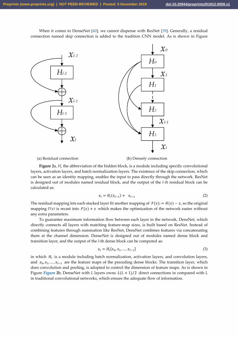
When it comes to DenseNet [40], we cannot dispense with ResNet [39]. Generally, a residual

connection named skip connection is added to the tradition CNN model. As is shown in Figure

Figure 2a, H, the abbreviation of the hidden block, is a module including specific convolutional

layers, activation layers, and batch normalization layers. The existence of the skip connection, which

can be seen as an identity mapping, enables the input to pass directly through the network. ResNet

is designed out of modules named residual block, and the output of the l-th residual block can be

calculated as:

𝑥𝑙 = 𝐻𝑙(𝑥𝑙−1) + 𝑥𝑙−1 (2)

The residual mapping lets each stacked layer fit another mapping of 𝐹(𝑥): = 𝐻(𝑥) − 𝑥, so the original

mapping F(x) is recast into 𝐹(𝑥) + 𝑥 which makes the optimization of the network easier without

any extra parameters.

To guarantee maximum information flow between each layer in the network, DensNet, which

directly connects all layers with matching feature-map sizes, is built based on ResNet. Instead of

combining features through summation like ResNet, DensNet combines features via concatenating

them at the channel dimension. DenseNet is designed out of modules named dense block and

transition layer, and the output of the l-th dense block can be computed as:

𝑥𝑙 = 𝐻𝑙[𝑥0, 𝑥1, … , 𝑥𝑙−1] (3)

in which 𝐻𝑙 is a module including batch normalization, activation layers, and convolution layers,

and 𝑥0, 𝑥1, … , 𝑥𝑙−1 are the feature maps of the preceding dense blocks. The transition layer, which

does convolution and pooling, is adopted to control the dimension of feature maps. As is shown in

Figure Figure 2b, DenseNet with L layers owns 𝐿(𝐿 + 1) 2⁄ direct connections in compared with L

in traditional convolutional networks, which ensure the adequate flow of information.



Figure 2. The architecture of Residual connection and Dense connection.

The structure of the dense block used in our framework can be seen in Figure Figure 3.

Supposing the size of the input feature maps as 𝑝 × 𝑝 × 𝑏 with n channels, then the output feature

maps of each composite convolution layer composed of k kernels in the shape of 1 × 1 × 𝑑 are 𝑝 ×

𝑝 × 𝑏 with k channels. However, as we know, dense connection concatenates feature maps at the

channel dimension, so the number of channels increases linearly with the number of composite

convolution layers. The channel’s quantity of a dense block with m layers can be formulated as:

𝑘𝑚 = 𝑏 + (𝑚 − 1) × 𝑘 (4)

where b is the channel’s index of the input feature maps.

2.2. The Measures Taken to Prevent Overfitting

A large number of training parameters and the limited number of training sets lead to the

tendency to overfit the seen data jointly. Next, we are going to elaborate on the measures taken to

prevent overfitting.

The activation function we adopted is Mish [48], a self-regularized non-monotonic activation

function, instead of the conventional ReLU [49]. The formula of the Mish is:

𝑚𝑖𝑠ℎ(𝑥) = 𝑥 × 𝑡𝑎𝑛ℎ(𝑠𝑜𝑓𝑡𝑝𝑙𝑢𝑠(𝑥)) = 𝑥𝑖 × 𝑡𝑎𝑛ℎ(𝑙𝑛(1 + 𝑒𝑥)) (5)

where x represents the input of the activation. The comparison of Mish and ReLU can be seen in

Figure Figure 4. Mish is lower bounded, and upper unbounded with a range [≈ −0.31, ∞). The

derivative of Mish is defined as:

𝑓′(𝑥) =𝑒𝑥𝜔

𝛿2 (6)

where 𝜔 = 4(𝑥 + 1) + 4𝑒𝑥 + 𝑒3𝑥 + 𝑒𝑥(4𝑥 + 6) and 𝛿 = 2𝑒𝑥 + 𝑒2𝑥 + 2.



Figure 3. The architecture of dense connection.

Figure 4. The comparison of the function graphs of Mish and ReLU.

As we know, the ReLU activation function defined as 𝑅𝑒𝐿𝑈(𝑥) = 𝑚𝑎𝑥(0, 𝑥) is a piecewise linear

function which prunes all the negative inputs. Moreover, the sparsity in the neural network is

induced by this property on account of if the input is nonpositive, then the neuron is going to “die”

and cannot be activated anymore, even though negative inputs might involve salutary information.

On the contrary, slight negative inputs are preserved as negative outputs by Mish, which tradeoffs

the input information and the network sparsity better.

A drop layer [50] is adopted between the last batch normalization layer and the global average

pooling layer in the spectral branch and spatial branch severally. Dropout is a simple but effective

technology to prevent overfitting by dropping out units (hidden or visible) on a given percentage p

at the training phase. Moreover, the p is selected as 0.5 in our framework. The existence of dropout

makes the presence of other units unreliable, which prevents co-adaptation between each unit.

Besides, two training skills, early stopping, and the dynamic learning rate are also introduced to

our model. Early stopping means if the loss is no longer decreasing for a certain number of epochs

(in our model, the number is 20), then we will stop the training process early to prevent overfitting

and reduce the training time meanwhile. For the sake of dynamical learning rate, the cosine annealing

[51] method is adopted to adjust the learning rate dynamically as the followed equation:



𝜂𝑡 = 𝜂𝑚𝑖𝑛𝑖 +

1

2(𝜂𝑚𝑎𝑥

𝑖 − 𝜂𝑚𝑖𝑛𝑖 ) (1 + cos (

𝑇𝑐𝑢𝑟

𝑇𝑖

𝜋)) (7)

where 𝜂𝑡 is the learning rate within the i-th run and [𝜂𝑚𝑖𝑛𝑖 , 𝜂𝑚𝑎𝑥

𝑖 ] is the range of the learning rate.

𝑇𝑐𝑢𝑟 accounts for the count of epochs that have been executed, and 𝑇𝑖 controls the count of epochs

that will be executed in a cycle of adjustment.

2.3. Attention Mechanism

Instead of processing a whole scenario across-the-board at once, human perception tends to pay

attention selectively to portions of the visual space in order to acquire information when and where

it is required and integrate information from various fixations over time to generate an internal

representation of the scenario [52]. Inspired by above-mentioned percipience, the attention

mechanism has been introduced in image categorization [53], and were later proved to be dominant

in the areas including Image Caption [54], Text to Image Synthesis [55] and Scene Segmentation [47],

et al. Obviously, diverse spectral channel and zones of different of the input patch make the

discrepant contribution to extracting features. Therefore, the attention mechanism can be adapted to

focus on the most compelling part and compress the inconsequential region’s weight.

Within our framework, feature maps generated by anterior dense spectral block and dense

spatial block are fed into spectral attention module and spatial attention module separately. By

spectral attention module, the weight of each spectrum is adjusted to highlight the informative

channel. Likewise, the spatial attention module makes discriminative areas at spatial dimension

prominent.

In DANet [47], after feeding the features into the spatial attention module, features of spatial

long-range contextual information are generated by three steps. In the first step, a spatial attention

matrix is computed, which models the spatial relationship between any two pixels of the features.

Next, a matrix multiplication between the original features and the attention matrix is performed.

Finally, an element-wise sum operation on the original features and the multiplied resulting matrix

is executed to obtain the final representation, which reflects long-range contexts. Similarly, long-

range contextual information in the channel dimension is extracted by a spectral attention module,

meanwhile just like the spatial attention module expects for the first step, in which the channel

attention matrix is calculated in channel dimension. Next, the two modules would be introduced in

detail.

2.3.1. Spatial Attention Module

Long-range contextual information is captured to obtain discriminant feature representations by

the spatial attention module. Against that, what features generated by conventional fully

convolutional networks (FCNs) considers merely is the local connection.

As illustrated in Figure Figure 5a, given a local feature 𝑨ℝ𝑐×𝑝×𝑝, two convolution layers are

adopted to generate new feature maps B and C severally where {𝑩, 𝑪}ℝ𝑐×𝑝×𝑝 (Note: Generally, the

height and width of the input feature maps are unequal values, but overall feature maps of our

framework are square in that we take the same patch size on the two dimensions to generate the

original data cube). Next, B and C are reshaped into ℝ𝑐×𝑛 where 𝑛 = 𝑝 × 𝑝 is the count of pixels.

Then a matrix multiplication is executed between B and C, and a softmax layer is attached

subsequently to compute the spatial attention map 𝑺ℝ𝑛×𝑛:

𝑠𝑗𝑖 =𝑒𝑥𝑝(𝐵𝑖×𝐶𝑗)

∑ 𝑒𝑥𝑝(𝐵𝑖×𝐶𝑗)𝑁𝑖=1

(8)

where 𝑠𝑗𝑖 measures the i-th position’s impact on the j-th position. The more similar feature

representations of the two positions are, the stronger the correlation between them is.

Meanwhile, the initial input feature A is fed into a convolution layer to obtain a new feature map

𝑫ℝ𝑐×𝑝×𝑝 which is reshaped into ℝ𝑐×𝑛 whereafter. Then a matrix multiplication is performed

between D and 𝐒𝐓, and the result is reshaped into ℝ𝑐×𝑝×𝑝 as:



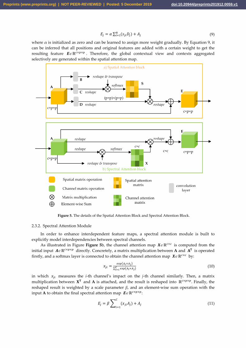
𝐸𝑗 = 𝛼 ∑ (𝑠𝑗𝑖𝐷𝑗) + 𝐴𝑗𝑁𝑖=1 (9)

where α is initialized as zero and can be learned to assign more weight gradually. By Equation 9, it

can be inferred that all positions and original features are added with a certain weight to get the

resulting feature 𝑬ℝ𝑐×𝑝×𝑝 . Therefore, the global contextual view and contexts aggregated

selectively are generated within the spatial attention map.

Figure 5. The details of the Spatial Attention Block and Spectral Attention Block.

2.3.2. Spectral Attention Module

In order to enhance interdependent feature maps, a spectral attention module is built to

explicitly model interdependencies between spectral channels.

As illustrated in Figure Figure 5b, the channel attention map 𝑿ℝ𝑐×𝑐 is computed from the

initial input 𝑨ℝ𝑐×𝑝×𝑝 directly. Concretely, a matrix multiplication between A and 𝐀𝐓 is operated

firstly, and a softmax layer is connected to obtain the channel attention map 𝑿ℝ𝑐×𝑐 by:

𝑥𝑗𝑖 =𝑒𝑥𝑝(𝐴𝑖×𝐴𝑗)

∑ 𝑒𝑥𝑝(𝐴𝑖×𝐴𝑗)𝐶𝑖=1

(10)

in which 𝑥𝑗𝑖 measures the i-th channel’s impact on the j-th channel similarly. Then, a matrix

multiplication between 𝐗𝐓 and A is attached, and the result is reshaped into ℝ𝑐×𝑝×𝑝. Finally, the

reshaped result is weighted by a scale parameter β, and an element-wise sum operation with the

input A to obtain the final spectral attention map 𝑬ℝ𝑐×𝑝×𝑝:

𝐸𝑗 = 𝛽 ∑ (𝑥𝑗𝑖𝐴𝑗) + 𝐴𝑗

𝐶

𝑖=1 (11)



where β is initialized as zero and can be learned gradually. Similarly, the final map E is obtained by

the weighted sum of all channels’ feature, which can describe the long-range dependencies and boost

the discriminability about features.

2.4. The Structure of the DBDA network.

The whole structure of the DBDA network can be seen in Figure Figure 6, and then we will

elaborate on the whole process in detail.

2.4.1. Spectral Branch with Channel Attention Block

Just taking the Indian Pines dataset as an example, and the input patch size is set to 9 × 9 × 200.

In the Spectral Branch, a 3D convolutional layer with 24 channels whose kernel size is 1 × 1 × 7 is

used, and the stride is set to (1,1,2) that can compress the count of channels. So, we can get the

feature maps in the shape of (9 × 9 × 97,24). Then, the dense spectral block combined by three

convolutional layers with a batch normalization layer is attached. And each convolutional layer has

12 channels in the shape of 1 × 1 × 7, and the stride is set to (1,1,1). Calculated by Equation (4), we

can obtain the feature maps with 60 channels. After traversing the last 3D convolutional layer in the

shape of (1 × 1 × 97,60), a (9 × 9 × 1,60) feature map is generated. Due to the 60 channels make

different contributions to the classification, a channel attention block, as illustrated in Figure Figure

5b and expatiated in Section 2.3.2, is adopted, which reinforces the informative channels and whittle

informative-lacking channels. After obtaining the weighted spectral feature maps, a batch

normalization layer and a drop layer are applied to enhance the numerical stability and vanquish the

overfitting. Finally, we can gain a spectral feature with a size of 1 × 60 via a Global Average Pooling

layer. The details of the structure can be seen in Table Table 1.

Table 1. The network structure of Spectral Branch.

Layer name Kernel Size Output Size

Input - (9 × 9 × 200)

Conv (1× 1 × 7) (9 × 9 × 97,24)

BN-Mish-Conv (1× 1 × 7) (9 × 9 × 97,12)

Concatenate - (9 × 9 × 97,36)

BN-Mish-Conv (1× 1 × 7) (9 × 9 × 97,12)

Concatenate - (9 × 9 × 97,48)

BN-Mish-Conv (1× 1 × 7) (9 × 9 × 97,12)

Concatenate - (9 × 9 × 97,60)

BN-Mish-Conv (1× 1 × 97) (9 × 9 × 1,60)

Channel Attention Block - (9 × 9 × 1,60)

BN-Drop-GlobalAveragePooling - (1 × 60)



Figure 6. The structure of the DBDA network. The top branch, Spectral Branch composed of the dense

spectral block and channel attention block, is designed to capture spectral features. The bottom

branch, Spatial Branch constituted by dense spatial block, and spatial attention block is designed to

extract spatial features.



2.4.2. Spatial Branch with Spatial Attention Block

Meanwhile, the input data in the shape of 9 × 9 × 200 are delivered to the Spatial Branch, and

the initial 3D convolutional layer’s size is set to 1 × 1 × 200, which can eliminate spectral channels.

After that, we can obtain feature maps in the shape of (9 × 9 × 1,24). Analogously, the dense spectral

block combined by three convolutional layers with a batch normalization layer is attached. And each

convolutional layer has 12 channels in the shape of 3 × 3 × 1, and the stride is set to (1,1,1). Next,

the extracted feature maps with the size of (9 × 9 × 1,60) are fed into the spatial attention block, as

illustrated in Figure Figure 5a and expound in Section 2.3.1, in which the coefficient of each pixel is

weighed to get a more discriminative spatial feature. After capturing the weighted spatial feature

maps, a batch normalization layer and a drop layer are applied to heighten the numerical stability

and defeat the overfitting. Finally, we can gain a spatial feature with a size of 1 × 60 via a Global

Average Pooling layer. The details of the structure can be seen in Table Table 2.

2.4.3. Spectral-Spatial Fusion for Classification

The spectral feature and spatial feature are obtained by the Spectral Branch and Spatial Branch

severally. Then, we perform a concatenation between two features for classification. Moreover, the

reason why the concatenation is applied instead of add operation is that the spectral feature and

spatial feature are in the disparate domain, but the add operation will mingle spectral and spatial

features. In the end, the conclusive classification result is obtained via the fully connected layer and

softmax activation.

For other datasets, network implementation details are executed in the same way, and the only

difference is the number of bands.

Table 2. The network structure of the Spatial Branch.

Layer name Kernel Size Output Size

Input - (9 × 9 × 200)

Conv (1× 1 × 200) (9 × 9 × 1,24)

BN-Mish-Conv (3× 3 × 1) (9 × 9 × 1,12)

Concatenate - (9 × 9 × 1,36)

BN-Mish-Conv (3× 3 × 1) (9 × 9 × 1,12)

Concatenate - (9 × 9 × 1,48)

BN-Mish-Conv (3× 3 × 1) (9 × 9 × 1,12)

Concatenate - (9 × 9 × 1,60)

Channel Attention Block - (9 × 9 × 1,60)

BN-Drop-GlobalAveragePooling - (1 × 60)

3. Datasets Introduction and Experimental Setting

3.1. Datasets Introduction

In the experiments, four widely used HSI datasets, the Indian Pines (IP) dataset, the Pavia

University (UP) dataset, the Salinas Valley (SV) dataset, and the Botswana dataset (BS), are employed

to measure the accuracy and efficiency of the proposed model. Three quantitative metrics, overall

accuracy (OA), average accuracy (AA), and Kappa coefficient (K), are used to assess the performance.

OA denotes the proportion of correct classifications to the total pixels to be classified. AA refers to

the average accuracy of all categories. Kappa coefficients can be used to verify the consistency and

can also be used to measure accuracy. The higher the three metric values are, the better the

classification consequence is.

Indian Pines (IP): The Indian Pines dataset was gathered by Airborne Visible/Infrared Imaging

Spectrometer (AVIRIS) sensor in North-western Indiana, composed of 200 spectral bands in the

wavelength range of 0.4 um to 2.5 um and 16 land cover classes. IP consists of 145 × 145 pixels, and

the resolution is 20 m/pixel.



Pavia University (UP): The Pavia University dataset was acquired by the reflective optics

imaging spectrometer (ROSIS-3) sensor from the University of Pavia, northern Italy, composed of 103

spectral bands in the wavelength range of 0.43 um to 0.86 um and nine land cover classes. UP consists

of 610 × 340 pixels, and the resolution is 1.3 m/pixel.

Salinas Valley (SV): The Salinas Valley dataset was collected by the AVIRIS sensor from Salinas

Valley, CA, USA, composed of 204 spectral bands in the wavelength range of 0.4 um to 2.5 um and

16 land cover classes. SV consists of 512 × 217 pixels, and the resolution is 3.7 m/pixel.

Botswana (BS): The Botswana dataset was captured by the NASA EO-1 satellite over the

Okavango Delta, Botswana, composed of 145 spectral bands in the wavelength range of 0.4 um to 2.5

um and 14 land cover classes. BS consists of 1476 × 256 pixels, and the resolution is 30 m/pixel.

3.2. Experimental Setting

In our experiment, to evaluate the effectiveness of DBDA, we compared the proposed

framework to other deep-learning-based classifier CDCNN [56], SSRN [41], FDSSC [42], and the state-

of-the-art Double-Branch Multi-Attention Mechanism Network (DBMA) [45]. Furthermore, a

conventional classifier, the SVM with RBF kernel [57], is also taken into comparison. The training

time and testing time results were measured via the same computer configured with 32 GB of

memory and an NVIDIA GeForce RTX 2080Ti GPU. All deep-learning-based classifiers were

implemented with PyTorch, and SVM was implemented with sklearn. Then, a brief introduction to

the above methods will be given separately.

Table 3. The number of training, validation, and test samples in the IP dataset.

Order Class Total number Train Val Test

1 Alfalfa 46 3 3 40

2 Corn-notill 1428 42 42 1344

3 Corn-mintill 830 24 24 782

4 Corn 237 7 7 223

5 Grass-pasture 483 14 14 455

6 Grass-trees 730 21 21 688

7 Grass-pasture-mowed 28 3 3 22

8 Hay-windrowed 478 14 14 450

9 Oats 20 3 3 14

10 Soybean-notill 972 29 29 914

11 Soybean-mintill 2455 73 73 2309

12 Soybean-clean 593 17 17 559

13 Wheat 205 6 6 193

14 Woods 1265 37 37 1191

15 Buildings-Grass-Trees-Drives 386 11 11 364

16 Stone-Steel-Towers 93 3 3 87

Total 10,249 307 307 9635

Table 4. The number of training, validation, and test samples in the UP dataset.


1 Asphalt 6631 33 33 6565

2 Meadows 18,649 93 93 18463

3 Gravel 2099 10 10 2079

4 Trees 3064 15 15 3034

5 Painted metal sheets 1345 6 6 1333

6 Bare Soil 5029 25 25 4979

7 Bitumen 1330 6 6 1318

8 Self-Blocking Bricks 3682 18 18 3646



9 Shadows 947 4 4 939

Total 42,776 210 210 42356

Table 5. The number of training, validation, and test samples in the SV dataset.


1 Brocoli-green-weeds-1 2009 10 10 1989

2 Brocoli-green-weeds-2 3726 18 18 3690

3 Fallow 1976 9 9 1958

4 Fallow-rough-plow 1394 6 6 1382

5 Fallow-smooth 2678 13 13 2652

6 Stubble 3959 19 19 3921

7 Celery 3579 17 17 3545

8 Grapes-untrained 11,271 56 56 11159

9 Soil-vinyard-develop 6203 31 31 6141

10 Corn-senesced-green-weeds 3278 16 16 3246

11 Lettuce-romaine-4wk 1068 5 5 1058




15 Vinyard-untrained 7268 36 36 7196

16 Vinyard-vertical-trellis 1807 9 9 1789

Total 54,129 263 263 53603

Table 6. The number of training, validation, and test samples in the BS dataset.


1 Water 270 3 3 264

2 Hippo grass 101 2 2 97

3 Floodplain grasses1 251 3 3 245

4 Floodplain grasses2 215 3 3 209

5 Reeds1 269 3 3 263

6 Riparian 269 3 3 263

7 Fierscar2 259 3 3 253

8 Island interior 203 3 3 197

9 Acacia woodlands 314 4 4 306

10 Acacia shrublands 248 3 3 242

11 Acacia grasslands 305 4 4 297

12 Short mopane 181 2 2 177

13 Mixed mopane 268 3 3 262

14 Exposed soils 95 1 1 93

Total 3248 40 40 3168

SVM: For SVM, all spectral bands are fed into SVM with a radial basis function (RBF) kernel.

CDCNN: The architecture of the CDCNN is rendered in [56], which is based on 2D CNN and

ResNet. The input data consists of 5 × 5 × L neighbors of each pixel, where L represents the number

of spectral bands.

SSRN: The architecture of the SSRN is expounded in [41], which is based on 3D CNN and

ResNet. The input data is composed of 7 × 7 × L neighbors of each pixel.

FDSSC: The architecture of the FDSSC is elaborated in [42], which is based on 3D CNN and

DenseNet. The size of the input is 9 × 9 × L.

DBMA: The architecture of the DBMA is set out in [42], which is based on 3D CNN, DenseNet,

and an attention mechanism. The input patch size is set to 7 × 7 × L.



For all we know, deep learning algorithms are data-driven, which rely on teeming labeled

training samples severely. The more data fed in training usually yields the higher test accuracy with

more time consumption and computation complexity followed. For the IP dataset, we choose 3%

training samples and 3% validation samples. As the samples are enough for each class of UP and SV,

we select 0.5% training samples and 0.5% validation samples. Furthermore, for BS, the proportion of

training samples and validation samples is set to 1.2%. (The reason why decimal appears is that the

number of samples in BS is sparse, so we set ratio as 1% with an operation of the ceiling.) To the best

of authors’ knowledge, it is the first time that so few samples are adopted to train and validate the

model hitherto. For example, 16%, 20%, 10 %, and 5% of the IP samples are chosen for training

CDCNN, SSRN, FDSSC, and DBMA in their papers, respectively.

For CDCNN, SSRN, FDSSC, DBMA, and our proposed method, the batch size is set to 16, and

the optimizer is Adam with a learning rate of 0.0005 and 200 epochs as the upper limit. The early

stopping strategy is adopted for each model, which means if the loss in the validation set does not

reduce for 20 epochs, the training stage will be terminated.

4. Experimental Results

In our experiment, SVM with RBF kernel [57], CDCNN [56], SSRN [41], FDSSC [42] and DBMA

[45] were compared with our proposed framework at the same computing platform configured with

32 GB of memory and an NVIDIA GeForce RTX 2080Ti GPU. Furthermore, all deep-learning-based

classifiers were implemented with PyTorch.

4.1. Classification Maps and Results

The results of each dataset are demonstrated in Table Table 7-Table 10, and the best class-

specific accuracy is in bold. Figure Figure 7-Figure 10 displays the classification maps of each method.

As can be seen both in the figures and tables, our method obtains the state-of-the-art results on four

datasets.

Within the scope of deep-learning-based methods, our experiments show that the proposed

DBDA framework is dramatically superior to the CDCNN, SSRN, FDSSC, and DBMA, and balances

the accuracy and efficiency better. SVM and CDCNN perform poorly at most of the datasets.

Although the DBMA has state-of-the-art accuracy claimed in [45], the DBMA presents inferior

performance than the FDSSC on the IP and UP dataset, which may owe to finite training samples

making overfitting become a significant influencing factor. For the IP dataset, UP dataset, SV dataset,

and BS dataset, the proposed model obtains 2.23%, 2.75%, 2.07%, and 2.81% ameliorations compared

with the DBMA.

What is more, the classification accuracies gained by proposed methods for each class in the IP,

UP, SV, and BS dataset are not less than 82%. Taking the class 7 in the IP dataset as an example, which

has only three training samples, our method performs well and obtains an acceptable consequence

92.59%, while the results of other methods (SVM: 56.10%, CDCNN: 0.00%, SSRN: 0.00%, FDSSC:

73.53%, and DBMA: 40.00%) are unpardonable seemingly.

Table 7. Class-specific results for the IP dataset using 3% training samples.

Class Color SVM CDCNN SSRN FDSSC DBMA Proposed

1 24.24 0.00 100.0 85.42 93.48 100.0

2 58.10 62.36 89.14 97.20 91.15 88.49

3 64.37 57.00 77.49 94.45 99.58 97.12

4 37.07 37.50 88.95 100.0 98.57 100.0

5 87.67 88.16 96.48 100.0 97.45 100.0

6 84.02 79.63 98.15 100.0 95.66 `97.18

7 56.10 0.00 0.00 73.53 40.00 92.59

8 89.62 84.02 84.54 99.78 100.0 99.78

9 21.21 0.00 0.00 100.0 38.10 100.0

10 65.89 37.50 92.07 89.25 85.98 89.87



11 62.32 53.25 90.89 93.97 94.39 99.33

12 52.40 42.96 84.19 95.41 89.92 98.50

13 94.30 49.47 98.47 100.0 99.48 96.02

14 90.15 76.71 94.56 93.14 92.81 93.22

15 63.96 62.60 84.11 90.61 89.66 96.99

16 98.46 83.70 91.40 96.55 96.55 94.38

OA 69.41 62.32 89.81 94.87 93.15 95.38

AA 65.62 50.93 79.40 94.33 87.67 96.47

kappa 0.6472 0.5593 0.8839 0.9414 0.9219 0.9474

Figure 7. Classification maps of the IP dataset with 3% training samples. (a) False-color image. (b)

ground-truth (GT). (c)–(h) The classification maps using different methods.

Table 8. Class-specific results for the UP dataset using 0.5% training samples.


1 82.87 85.74 99.15 99.43 91.66 89.03

2 88.07 94.45 98.06 98.57 97.65 98.32

3 70.84 32.59 96.64 100.0 99.78 98.70

4 95.61 97.46 99.86 99.20 97.66 98.42

5 92.24 99.10 99.85 99.92 99.63 99.78

6 76.98 80.88 96.88 98.17 82.52 98.57

7 68.98 88.83 73.24 93.64 87.04 95.84

8 71.14 66.19 82.36 74.61 88.55 89.47

9 99.89 96.01 100.0 99.79 95.51 99.89

OA 84.29 87.70 95.59 95.88 93.25 96.00

AA 82.96 82.36 94.01 95.93 93.00 96.45

kappa 0.7883 0.8359 0.9415 0.9453 0.9108 0.9467



Figure 8. Classification maps of the UP dataset with 0.5% training samples. (a) False-color image. (b)


Table 9. Class-specific results for the SV dataset using 0.5% training samples.


1 99.85 0.00 100.0 100.0 100.0 100.0

2 98.95 64.82 100.0 100.0 99.51 99.17

3 89.88 94.69 89.72 99.44 98.92 97.74

4 97.30 82.99 94.85 98.57 96.39 95.95

5 93.56 98.24 99.39 99.87 96.39 99.29

6 99.89 96.51 99.95 99.97 99.17 99.92

7 91.33 95.98 99.75 99.75 96.80 99.83

8 74.73 88.23 88.60 99.60 95.60 95.97

9 97.69 99.26 98.48 99.69 99.22 99.37

10 90.01 67.39 98.81 99.02 96.20 96.72

11 75.92 72.03 93.30 92.77 82.29 93.72

12 95.19 75.49 99.95 99.64 99.17 100.0

13 94.87 95.71 100.0 100.0 98.91 100.0

14 89.26 94.92 97.86 98.05 98.22 96.89

15 75.86 51.88 89.96 74.58 84.71 93.42

16 99.03 99.62 100.0 100.0 100.0 100.0

OA 88.09 77.79 94.72 94.99 95.44 97.51

AA 91.45 79.86 96.66 97.56 96.34 98.00

kappa 0.8671 0.7547 0.9412 0.9444 0.9493 0.9723



Figure 9. Classification maps of the SV dataset with 0.5% training samples. (a) False-color image. (b)


Table 10. Class-specific results for the BS dataset using 1.2% training samples.


1 100.0 94.60 94.95 97.41 97.77 95.64

2 97.56 68.64 100.0 98.95 88.89 98.99

3 86.35 81.11 91.42 100.0 100.0 100.0

4 63.51 65.45 97.34 93.03 92.51 91.30

5 84.33 89.10 92.42 80.74 93.51 95.58

6 61.27 69.28 66.39 84.93 68.94 82.23

7 82.09 80.07 100.0 84.62 100.0 100.0

8 63.46 89.36 100.0 93.36 96.10 95.63

9 63.53 55.53 90.75 88.44 85.15 96.50

10 65.74 81.69 86.83 99.59 97.60 98.79

11 93.91 92.48 100.0 99.67 99.66 99.67

12 90.70 90.91 100.0 100.0 97.79 100.0

13 73.62 88.59 94.83 81.59 100.0 100.0

14 92.98 100.0 100.0 100.0 100.0 100.0

OA 77.21 80.90 91.89 91.57 93.43 96.24

AA 79.93 81.92 93.92 93.02 94.14 96.74

kappa 0.7532 0.7930 0.9121 0.9086 0.9.89 0.9593



Figure 10. Classification maps of the BS dataset with 1.2% training samples. (a) False-color image. (b)


4.2. Investigation on Running Time

Tables Table 11-Table 14 list the running time of the six methods on the IP, UP, SV, and BS

datasets, respectively. From the tables above, we can see that the SVM-based method and 2D-CNN-

based method consume less time than 3D-CNN-based methods; the latter means larger input size

and more parameters generally. For our method, it spends less training time less than FDSSC and

DBMA and obtains better performance.

Table 11. Training and testing time of different methods on the IP datasets.

Dataset Method Training Times (s) Test Times (s)

Indian Pines

SVM 20.10 0.66

CDCNN 11.13 1.54

SSRN 46.03 2.71

FDSSC 105.05 4.86

DBMA 94.69 6.35

Proposed 69.83 5.60

Table 12. Training and testing time of different methods on the UP datasets.


Pavia University

SVM 3.38 2.29

CDCNN 10.26 4.92

SSRN 17.71 6.41

FDSSC 31.70 10.65

DBMA 21.48 14.67

Proposed 18.46 13.32

Table 13. Training and testing time of different methods on the SV datasets.


Salinas

SVM 9.35 3.89

CDCNN 9.82 6.14

SSRN 73.75 13.99

FDSSC 99.91 25.57

DBMA 105.30 31.82



Proposed 71.18 23.93

Table 14. Training and testing time of different methods on the BS datasets.


Botswana

SVM 0.93 0.15

CDCNN 11.10 1.33

SSRN 8.87 1.37

FDSSC 17.84 1.45

DBMA 13.67 2.04

Proposed 17.19 1.90

4.3. Investigation on the Number of Training Samples

As we mentioned, deep learning is a genre of data-driven algorithms, depending on superb

annotated data. In this part, the performance with different amount of training samples would be

investigated.

Figure Figure 11 shows the experiment results. For IP dataset and BS dataset, 0.5%, 1%, 3%, 5%

and 10% of samples are adopted as training set. For UP dataset and SV dataset, 0.1%, 0.5%, 1%, 5%

and 10% of samples are adopted as training set.

The accuracy increases in the wake of the increasing training samples, as we had expected. All

3D-based methods, including SSRN, FDSSC, DBMA, and proposed framework could obtain near-

perfect performances whose OA can reach or exceed 99%, as long as sufficient samples (maybe 10%

of the whole dataset) are rendered. At the same time, the performance gap between the disparate

model is diminished following the increasing training samples inch by inch. Nevertheless, our

method performs better than other methods, especially when samples are deficient, which means our

method could offer acceptable classification results with limited labeled data when the expenditure

of manual annotation is exorbitant.

4.4. Ablation Experiments

The utility of spatial attention mechanism and spectral attention mechanism is validated in the

ablation experiments, in which three simplified DBDA framework, i.e., without spectral attention and

spatial attention (denoted as without-attention), only with spatial attention (denoted as spatial-

attention) and only with spectral attention (denoted as spectral-attention) are investigated.

The existence of spatial attention mechanism and spectral attention mechanism does promote

the accuracy of four datasets, which can be concluded in Figure Figure 12. Furthermore, spatial

attention mechanism performs more apparent effect upon most occasions.

4.5. Discussion

In this part, we attempt cautiously to illustrate the reason why our proposed framework works

availably.

First, Dual Attention Network (DANet) [47], a flexible and adaptive self-attention mechanism

module, is utilized to amplify the distinctiveness of spectral and spatial features. By a channel

attention module and a position attention module, global dependencies in the spectral and spatial

dimensions can be captured respectively. Even though DANet was designed for Scene Segmentation,

the essence of Scene Segmentation and HSI classification can be viewed as classification at the pixel

level. Based on the insight mentioned above, we have faith that more researches on the combination

of these two fields would be implemented.

Second, Mish [48], a self-regularized non-monotonic activation function, is selected as the

activation function of our framework. Compared with the classic ReLU, despite the computational

complexity of Mish is higher than ReLU, the properties of Mish, including unbounded above,

bounded below, smoothness, and non-monotonicity all dedicate ameliorations of convergence,

which dose reduce time consumption prominently.



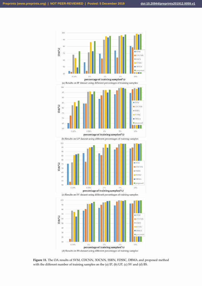
Figure 11. The OA results of SVM, CDCNN, 3DCNN, SSRN, FDSSC, DBMA and proposed method

with the different number of training samples on the (a) IP, (b) UP, (c) SV and (d) BS.



Figure 12. Ablation experiments about attention mechanisms on different datasets.

Third, dropout [50], a simple but effective skill to prevent overfitting, is affiliated to deal with

the contradictions between numerous initialized parameters and limited training samples. As we

analyzed earlier, DBMA [45] performs weaker than FDSSC [42] on two datasets when training

samples are restrictive, which might be caused by the lack of dropout layers in DBMA.

5. Conclusions

In this paper, an end-to-end Double-Branch Dual-Attention mechanism network was proposed

for HSI classification, which is equipped with two branches to capture spectral feature and spatial

feature severally and densely connected 3D convolution layer to retard the disappearance of the

gradient. Instead of cumbersome mechanism for reducing the dimensionality, we take the untreated

3D pixel data directly as input. Our work is based on the DBMA and DANet. DBMA is the state-of-

the-art algorithm in HSI classification, and DANet is a flexible and adaptive self-attention mechanism

in Scene Segmentation. Seemingly, a minor amelioration is obtained merely in this paper, but

numerous empirical researches demonstrate that our proposed framework surpassed other state-of-

the-art methods, especially when training samples are limited. Meanwhile, the consumption on time

is also decreased contrasted with FDSSC and DBMA, as the attention blocks and the activation

function Mish accelerate the convergence of the model.

The future direction of our work is generalizing our proposed framework to pragmatic

hyperspectral data acquired recently, not just on the above-mentioned open-source datasets.

Moreover, it is also an attractive challenge about how to compress the training time ulteriorly.

Acknowledgments: As this is the first time the first author, Rui Li, has written an article in English, in order to

finish the draft as soon as possible, we take two papers that owned the same direction, Double-Branch Multi-

Attention Mechanism Network for Hyperspectral Image Classification and A Fast Dense Spectral–Spatial Convolution

Network Framework for Hyperspectral Images Classification, for reference. Therefore, the duplicate rate checking is a

little high, maybe 30%, and we are revising our paper to the best of our ability. Thanks a million for the authors

of the abovementioned papers, they are Wenping Ma, Qifan Yang, Yue Wu, Wei Zhao and Xiangrong Zhang

who are the authors of the first paper, and Wenju Wang, Shuguang Dou, Zhongmin Jiang and Liujie Sun who

are the authors of the second paper.

Funding: This research was funded by the National Natural Science Foundations of China (Nos. 41671452)

Conflicts of Interest: The authors declare no conflicts of interest. The founding sponsors had no role in the

design of the study; in the collection, analyses, or interpretation of data; in the writing of the manuscript; nor in

the decision to publish the results.

References



1. Zhong, Y.; Ma, A.; Ong, Y.; Zhu, Z; Zhang, L. Computational intelligence in optical remote sensing image

processing. Applied Soft Computing, 2018, 64: 75-93.

2. Mahdianpari, M.; Salehi, B.; Rezaee, M.; Mohammadimanesh, F.; Zhang, Y. Very deep convolutional neural

networks for complex land cover mapping using multispectral remote sensing imagery. Remote Sensing,

2018, 10(7): 1119.

3. Pipitone, C.; Maltese, A.; Dardanelli, G.; Brutto, M.; Loggia, G. Monitoring water surface and level of a

reservoir using different remote sensing approaches and comparison with dam displacements evaluated

via GNSS. Remote Sensing, 2018, 10(1): 71.

4. Zhao, C.; Wang Y.; Qi B.; Wang J. Global and local real-time anomaly detectors for hyperspectral remote

sensing imagery. Remote Sensing, 2015, 7(4): 3966-3985.

5. Li, Z.; Huang, L.; He, J. A Multiscale Deep Middle-level Feature Fusion Network for Hyperspectral

Classification. Remote Sensing, 2019, 11(6): 695.

6. Awad, M.; Jomaa, I.; Arab, F. Improved Capability in Stone Pine Forest Mapping and Management in

Lebanon Using Hyperspectral CHRIS-Proba Data Relative to Landsat ETM+. Photogrammetric

Engineering & Remote Sensing, 2014, 80(8): 725-731.

7. Ibrahim, A.; Franz, B.; Ahmad, Z.; Healy R.; Knobelspiesse, K.; Gao, B.; Proctor, C.; Zhai, P. Atmospheric

correction for hyperspectral ocean color retrieval with application to the Hyperspectral Imager for the

Coastal Ocean (HICO). Remote Sensing of Environment, 2018, 204: 60-75.

8. Marinelli, D.; Bovolo, F.; Bruzzone, L. A novel change detection method for multitemporal hyperspectral

images based on binary hyperspectral change vectors. IEEE Transactions on Geoscience and Remote

Sensing, 2019.

9. Melgani, F.; Bruzzone, L. Classification of hyperspectral remote sensing images with support vector

machines. IEEE Transactions on geoscience and remote sensing, 2004, 42(8): 1778-1790.

10. Li, J.; Bioucas-Dias, J.; Plaza, A. Semisupervised hyperspectral image segmentation using multinomial

logistic regression with active learning. IEEE Transactions on Geoscience and Remote Sensing, 2010, 48(11):

4085-4098.

11. Li, J.; Bioucas-Dias, J.; Plaza, A. Spectral–spatial hyperspectral image segmentation using subspace

multinomial logistic regression and Markov random fields. IEEE Transactions on Geoscience and Remote

Sensing, 2011, 50(3): 809-823.

12. Du, B.; Zhang, L. Random-selection-based anomaly detector for hyperspectral imagery. IEEE Transactions

on Geoscience and Remote Sensing, 2010, 49(5): 1578-1589.

13. Du, B.; Zhang, L. Target detection based on a dynamic subspace. Pattern Recognition, 2014, 47(1): 344-358.

14. Li, J.; Marpu, P.; Plaza, A.; Bioucas-Dias, J.; Benediktsson, J. Generalized composite kernel framework for

hyperspectral image classification. IEEE transactions on geoscience and remote sensing, 2013, 51(9): 4816-

4829.

15. Li, W.; Du, Q. Gabor-filtering-based nearest regularized subspace for hyperspectral image classification.

IEEE Journal of Selected Topics in Applied Earth Observations and Remote Sensing, 2014, 7(4): 1012-1022.

16. Fang, L.; Li, S.; Duan, W.; Ren, J.; Benediktsson, J. Classification of hyperspectral images by exploiting

spectral–spatial information of superpixel via multiple kernels. IEEE transactions on geoscience and remote

sensing, 2015, 53(12): 6663-6674.

17. Camps-Valls, G.; Gomez-Chova, L.; Muñoz-Marí, J.; Vila-Frances, J.; Calpe-Maravilla, J. Composite kernels

for hyperspectral image classification. IEEE geoscience and remote sensing letters, 2006, 3(1): 93-97.

18. Fang, L.; He, N.; Li, S.; Ghamisi. P.; Benediktsson, J. Extinction profiles fusion for hyperspectral images

classification. IEEE Transactions on Geoscience and Remote Sensing, 2017, 56(3): 1803-1815.

19. Li, P.; Chen, X.; Shen, S. Stereo r-cnn based 3d object detection for autonomous driving. Proceedings of the

IEEE Conference on Computer Vision and Pattern Recognition. 2019: 7644-7652.

20. Zhang, W.; Feng, Y.; Meng, F.; You D.; Liu Q. Bridging the Gap between Training and Inference for Neural

Machine Translation. arXiv preprint arXiv:1906.02448, 2019.

21. Durand, T.; Mehrasa, N.; Mori, G. Learning a Deep ConvNet for Multi-label Classification with Partial

Labels. Proceedings of the IEEE Conference on Computer Vision and Pattern Recognition. 2019: 647-657.

22. Chen, Y.; Lin, Z.; Zhao, X.; Wang G.; Gu Y. Deep learning-based classification of hyperspectral data. IEEE

Journal of Selected topics in applied earth observations and remote sensing, 2014, 7(6): 2094-2107.

23. Tao, C.; Pan, H.; Li, Y.; Zou Z. Unsupervised spectral–spatial feature learning with stacked sparse

autoencoder for hyperspectral imagery classification. IEEE Geoscience and remote sensing letters, 2015,

12(12): 2438-2442.



24. Ma, X.; Wang, H.; Geng, J. Spectral–spatial classification of hyperspectral image based on deep auto-

encoder. IEEE Journal of Selected Topics in Applied Earth Observations and Remote Sensing, 2016, 9(9):

4073-4085.

25. Zhang, X.; Liang, Y.; Li, C.; Hu, N.; Jiao, L; Zhou, H. Recursive autoencoders-based unsupervised feature

learning for hyperspectral image classification. IEEE Geoscience and Remote Sensing Letters, 2017, 14(11):

1928-1932.

26. Chen, Y.; Zhao, X.; Jia, X. Spectral–spatial classification of hyperspectral data based on deep belief network.

IEEE Journal of Selected Topics in Applied Earth Observations and Remote Sensing, 2015, 8(6): 2381-2392.

27. Makantasis, K.; Karantzalos, K.; Doulamis, A.; Doulamis, D. Deep supervised learning for hyperspectral

data classification through convolutional neural networks. 2015 IEEE International Geoscience and Remote

Sensing Symposium (IGARSS). IEEE, 2015: 4959-4962.

28. Zhao, W.; Du, S. Spectral–spatial feature extraction for hyperspectral image classification: A dimension

reduction and deep learning approach[J]. IEEE Transactions on Geoscience and Remote Sensing, 2016,

54(8): 4544-4554.

29. Chen, Y.; Jiang, H.; Li, C.; Jia, X.; Ghamisi P. Deep feature extraction and classification of hyperspectral

images based on convolutional neural networks. IEEE Transactions on Geoscience and Remote Sensing,

2016, 54(10): 6232-6251.

30. Li, Y.; Zhang, H.; Shen, Q. Spectral–spatial classification of hyperspectral imagery with 3D convolutional

neural network. Remote Sensing, 2017, 9(1): 67.

31. Mou, L.; Ghamisi, P.; Zhu X. Deep recurrent neural networks for hyperspectral image classification. IEEE

Transactions on Geoscience and Remote Sensing, 2017, 55(7): 3639-3655.

32. Tan, K.; Hu, J.; Li, J.; Du P. A novel semi-supervised hyperspectral image classification approach based on

spatial neighborhood information and classifier combination. ISPRS journal of photogrammetry and

remote sensing, 2015, 105: 19-29.

33. Zhang, M.; Gong, M; Mao, Y; Li, J.; Wu, Y. Unsupervised feature extraction in hyperspectral images based

on wasserstein generative adversarial network. IEEE Transactions on Geoscience and Remote Sensing,

2018, 57(5): 2669-2688.

34. Haut, J.; Paoletti, M.; Plaza, J.; Li J.; Plaza, A. Active learning with convolutional neural networks for

hyperspectral image classification using a new bayesian approach. IEEE Transactions on Geoscience and

Remote Sensing, 2018, 56(11): 6440-6461.

35. Paoletti, M.; Haut, J.; Fernandez-Beltran, R.; Plaza, J.; Plaza, A.; Li, Jun.; Pla, F. Capsule networks for

hyperspectral image classification. IEEE Transactions on Geoscience and Remote Sensing, 2018, 57(4): 2145-

2160.

36. Yang, S.; Feng, Z.; Wang, M.; Zhang, K. Self-paced learning-based probability subspace projection for

hyperspectral image classification. IEEE transactions on neural networks and learning systems, 2018, 30(2):

630-635.

37. Kemker, R.; Kanan, C. Self-taught feature learning for hyperspectral image classification. IEEE Transactions

on Geoscience and Remote Sensing, 2017, 55(5): 2693-2705.

38. Chen, Z.; Jiang, J.; Zhou, C.; Fu S.; Cai, Z. SuperBF: Superpixel-Based Bilateral Filtering Algorithm and Its

Application in Feature Extraction of Hyperspectral Images. IEEE Access, 2019, 7: 147796-147807.

39. He, K.; Zhang, X.; Ren, S.; Sun, J. Deep residual learning for image recognition. Proceedings of the IEEE

conference on computer vision and pattern recognition. 2016: 770-778.

40. Huang, G.; Liu, Z.; Maaten, L.; Weinberger, K. Densely connected convolutional networks. Proceedings of

the IEEE conference on computer vision and pattern recognition. 2017: 4700-4708.

41. Zhong, Z.; Li, J.; Luo, Z.; Chapman, M.; Weinberger Q. Spectral–spatial residual network for hyperspectral

image classification: A 3-D deep learning framework. IEEE Transactions on Geoscience and Remote

Sensing, 2017, 56(2): 847-858.

42. Wang, W.; Dou, S.; Jiang, Z.; Sun L. A Fast Dense Spectral–Spatial Convolution Network Framework for

Hyperspectral Images Classification. Remote Sensing, 2018, 10(7): 1068.

43. Fang, B.; Li, Y.; Zhang, H.; Chan, J. Hyperspectral Images Classification Based on Dense Convolutional

Networks with Spectral-Wise Attention Mechanism. Remote Sensing, 2019, 11(2): 159.

44. Woo, S.; Park, J.; Lee, J.; Kweon, I. Cbam: Convolutional block attention module. Proceedings of the

European Conference on Computer Vision (ECCV). 2018: 3-19.

45. Ma, W.; Yang, Q.; Wu, Y.; Zhao, W.; Zhang X. Double-Branch Multi-Attention Mechanism Network for

Hyperspectral Image Classification. Remote Sensing, 2019, 11(11): 1307.



46. Hou, R.; Chang, H.; Ma, B.; Shan, S.; Chen, X. Cross Attention Network for Few-shot Classification. arXiv

preprint arXiv:1910.07677, 2019.

47. Fu, J.; Liu, J.; Tian, H.; Li, Y.; Bao, Y.; Fang, Z.; Lu H. Dual attention network for scene segmentation.

Proceedings of the IEEE Conference on Computer Vision and Pattern Recognition. 2019: 3146-3154.

48. Misra, D. Mish: A Self Regularized Non-Monotonic Neural Activation Function. arXiv preprint

arXiv:1908.08681, 2019.

49. Krizhevsky, A.; Sutskever, I.; Hinton, G. Imagenet classification with deep convolutional neural networks.

Advances in neural information processing systems. 2012: 1097-1105.

50. Srivastava, N.; Hinton, G.; Krizhevsky, A.; Sutskever, I.; Salakhutdinov, R. Dropout: a simple way to

prevent neural networks from overfitting. The journal of machine learning research, 2014, 15(1): 1929-1958.

51. Loshchilov, I.; Hutter, F. Sgdr: Stochastic gradient descent with warm restarts. arXiv preprint

arXiv:1608.03983, 2016.

52. Rensink, R. The dynamic representation of scenes. Visual cognition, 2000, 7(1-3): 17-42.

53. Mnih, V.; Heess, N.; Graves A. Recurrent models of visual attention. Advances in neural information

processing systems. 2014: 2204-2212.

54. Xu, K.; Ba, J.; Kiros, R.; Cho, K.; Courville, A.; Salakhutdinov, R.; Zemel, R.; Bengio, Y. Show, attend and

tell: Neural image caption generation with visual attention. International conference on machine learning.

2015: 2048-2057.

55. Xu, T.; Zhang, P.; Huang, Q.; Zhang, H.; Gan, Z.; Huang, X.; He, X. Attngan: Fine-grained text to image

generation with attentional generative adversarial networks. Proceedings of the IEEE Conference on

Computer Vision and Pattern Recognition. 2018: 1316-1324.

56. Lee, H.; Kwon, H. Going deeper with contextual CNN for hyperspectral image classification. IEEE

Transactions on Image Processing, 2017, 26(10): 4843-4855.

57. Melgani, F.; Bruzzone. L. Classification of hyperspectral remote sensing images with support vector

machines. IEEE Transactions on geoscience and remote sensing, 2004, 42(8): 1778-1790.



article classification of hyperspectral image based on

Documents