Article

Comparison of prestellar core elongations and large­scale molecular cloud structures in the Lupus 1 region

Poidevin, Frédérick, Ade, Peter A. R., Angile, Francesco E., Benton, Steven J., Chapin, Edward L., Devlin, Mark J., Fissel, Laura M., Fukui, Yasuo, Gandilo, Natalie N., Gundersen, Joshua O., Hargrave, Peter C., Klein, Jeffrey, Korotkov, Andrei L., Matthews, Tristan G., Moncelsi, Lorenzo, Mroczkowski, Tony K., Netterfield, Calvin B., Novak, Giles, Nutter, David, Olmi, Luca, Pascale, Enzo, Savini, Giorgio, Scott, Douglas, Shariff, Jamil A., Soler, Juan Diego, Tachihara, Kengo, Thomas, Nicholas E., Truch, Matthew D. P., Tucker, Carole E., Tucker, Gregory S. and Ward-Thompson, Derek

Available at http://clok.uclan.ac.uk/11723/

Poidevin, Frédérick, Ade, Peter A. R., Angile, Francesco E., Benton, Steven J., Chapin, Edward L., Devlin, Mark J., Fissel, Laura M., Fukui, Yasuo, Gandilo, Natalie N. et al (2014) Comparison of prestellar core elongations and large­scale molecular cloud structures in the Lupus 1 region. Astrophysical Journal, 791 (1). p. 43. ISSN 0004­637X  

It is advisable to refer to the publisher’s version if you intend to cite from the work.http://dx.doi.org/10.1088/0004-637x/791/1/43

For more information about UCLan’s research in this area go to http://www.uclan.ac.uk/researchgroups/ and search for <name of research Group>.

For information about Research generally at UCLan please go to http://www.uclan.ac.uk/research/

All outputs in CLoK are protected by Intellectual Property Rights law, includingCopyright law. Copyright, IPR and Moral Rights for the works on this site are retained by the individual authors and/or other copyright owners. Terms and conditions for use of this material are defined in the http://clok.uclan.ac.uk/policies/

CLoKCentral Lancashire online Knowledgewww.clok.uclan.ac.uk

The Astrophysical Journal, 791:43 (9pp), 2014 August 10 doi:10.1088/0004-637X/791/1/43C© 2014. The American Astronomical Society. All rights reserved. Printed in the U.S.A.

COMPARISON OF PRESTELLAR CORE ELONGATIONS AND LARGE-SCALE MOLECULAR CLOUDSTRUCTURES IN THE LUPUS I REGION

Frederick Poidevin1,2,3, Peter A. R. Ade4, Francesco E. Angile5, Steven J. Benton6, Edward L. Chapin7,Mark J. Devlin5, Laura M. Fissel8,9, Yasuo Fukui10, Natalie N. Gandilo8, Joshua O. Gundersen11, Peter C. Hargrave4,

Jeffrey Klein5, Andrei L. Korotkov12, Tristan G. Matthews9,13, Lorenzo Moncelsi14, Tony K. Mroczkowski14,Calvin B. Netterfield6,8, Giles Novak9,13, David Nutter4, Luca Olmi15,16, Enzo Pascale4, Giorgio Savini1,

Douglas Scott17, Jamil A. Shariff8, Juan Diego Soler8,18, Kengo Tachihara10, Nicholas E. Thomas11,Matthew D. P. Truch5, Carole E. Tucker4, Gregory S. Tucker12, and Derek Ward-Thompson19

1 UCL, KLB, Department of Physics & Astronomy, Gower Place, London WC1E 6BT, UK2 Instituto de Astrofısica de Canarias, E-38200 La Laguna, Tenerife, Spain; fpoidevin@iac.es

3 Dept. Astrofısica, Universidad de La Laguna, E-38206 La Laguna, Tenerife, Spain4 School of Physics and Astronomy, Cardiff University, Queens Buildings, The Parade, Cardiff CF24 3AA, UK

5 Department of Physics and Astronomy, University of Pennsylvania, 209 South 33rd Street, Philadelphia, PA 19104, USA6 Department of Physics, University of Toronto, 60 St. George Street, Toronto, ON M5S 1A7, Canada

7 XMM SOC, ESAC, Apartado 78, E-28691 Villanueva de la Canada, Madrid, Spain8 Department of Astronomy and Astrophysics, University of Toronto, 50 St. George Street, Toronto, ON M5S 3H4, Canada

9 Department of Physics and Astronomy, Northwestern University, 2145 Sheridan Road, Evanston, IL 60208, USA10 Department of Physics, Nagoya University, Chikusa-ku, Nagoya, Aichi 464-8601, Japan

11 Department of Physics, University of Miami, 1320 Campo Sano Drive, Coral Gables, FL 33146, USA12 Department of Physics, Brown University, 182 Hope Street, Providence, RI 02912, USA

13 Center for Interdisciplinary Exploration and Research in Astrophysics (CIERA), Northwestern University, 2145 Sheridan Road, Evanston, IL 60208, USA14 California Institute of Technology, 1200 East California Boulevard, Pasadena, CA 91125, USA

15 Physics Department, University of Puerto Rico, Rio Piedras Campus, Box 23343, UPR station, San Juan, PR 00931, USA16 Osservatorio Astrofisico de Arcetri, INAF, Largo E. Fermi 5, I-50125 Firenze, Italy

17 Department of Physics and Astronomy, University of British Colombia, 6224 Agricultural Road, Vancouver, BC V6T 1Z1, Canada18 CNRS-Institut d’Astrophysique Spatiale, Universite Paris-XI, F-91405 Orsay, France

19 Jeremiah Horrocks Institute, University of Central Lancashire, PR1 2HE, UKReceived 2014 April 30; accepted 2014 June 24; published 2014 July 24

ABSTRACT

Turbulence and magnetic fields are expected to be important for regulating molecular cloud formation and evolution.However, their effects on sub-parsec to 100 parsec scales, leading to the formation of starless cores, are not wellunderstood. We investigate the prestellar core structure morphologies obtained from analysis of the Herschel-SPIRE350 μm maps of the Lupus I cloud. This distribution is first compared on a statistical basis to the large-scale shapeof the main filament. We find the distribution of the elongation position angle of the cores to be consistent with arandom distribution, which means no specific orientation of the morphology of the cores is observed with respectto the mean orientation of the large-scale filament in Lupus I, nor relative to a large-scale bent filament model.This distribution is also compared to the mean orientation of the large-scale magnetic fields probed at 350 μm withthe Balloon-borne Large Aperture Telescope for Polarimetry during its 2010 campaign. Here again we do not findany correlation between the core morphology distribution and the average orientation of the magnetic fields onparsec scales. Our main conclusion is that the local filament dynamics—including secondary filaments that oftenrun orthogonally to the primary filament—and possibly small-scale variations in the local magnetic field direction,could be the dominant factors for explaining the final orientation of each core.

Key words: ISM: clouds – ISM: individual objects (Lupus I) – ISM: magnetic fields – polarization –submillimeter: ISM

Online-only material: color figures

1. INTRODUCTION

Understanding the processes leading to the formation of starsin our Galaxy is one of the great challenges which, despite muchprogress (e.g., Molinari et al. 2014), still remains open. At sub-parsec scales, the detailed mechanisms remain elusive throughwhich gravitational collapse occurs, leading to the formationof a prestellar core which eventually will give birth to one ormore stars. Recent advances have shown that turbulence is a keyingredient and plays a dual role, both creating overdensities toinitiate core formation and counteracting the effects of gravityinto the denser regions of these objects (e.g., McKee & Ostriker2007). In addition to gravity and turbulence, other physicalprocesses are likely to play a significant role. Specifically,

magnetic field and dynamical chemistry networks are expectedto be relevant for understanding the general phenomenologyof star formation (see, for example, Leao et al. 2013; Girartet al. 2013; Tassis et al. 2012a, 2012b, 2012c, and referencestherein). However, all in all, it is currently unclear which ofall these mechanisms dominates over the other ones, and overwhich spatial and temporal scales.

On larger spatial scales, the formation and evolution of molec-ular clouds is not well understood and there is abundant litera-ture on the subject. In particular, several simulation approachesaddressing these questions have been developed over the lasttwo decades (e.g., Ostriker et al. 2001; Gammie et al. 2003;Falceta-Goncalves et al. 2008; Heitsch et al. 2009; Nakamura &Li 2011; Bonnell et al. 2013). While these analyses sometimes

1

The Astrophysical Journal, 791:43 (9pp), 2014 August 10 Poidevin et al.

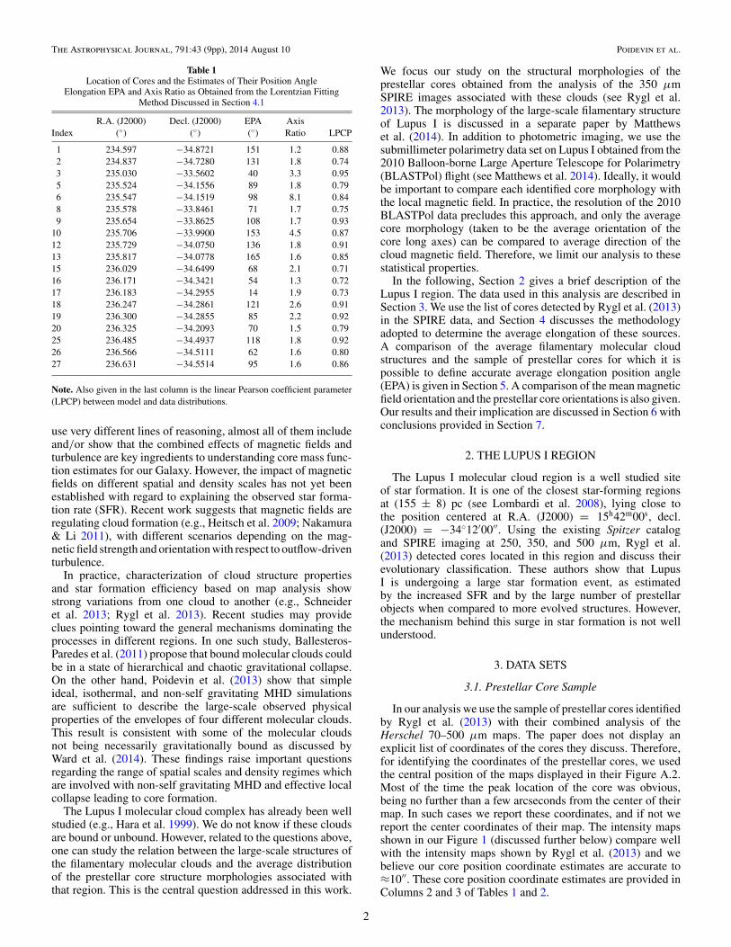
Table 1Location of Cores and the Estimates of Their Position Angle

Elongation EPA and Axis Ratio as Obtained from the Lorentzian FittingMethod Discussed in Section 4.1

R.A. (J2000) Decl. (J2000) EPA AxisIndex (◦) (◦) (◦) Ratio LPCP

1 234.597 −34.8721 151 1.2 0.882 234.837 −34.7280 131 1.8 0.743 235.030 −33.5602 40 3.3 0.955 235.524 −34.1556 89 1.8 0.796 235.547 −34.1519 98 8.1 0.848 235.578 −33.8461 71 1.7 0.759 235.654 −33.8625 108 1.7 0.93

10 235.706 −33.9900 153 4.5 0.8712 235.729 −34.0750 136 1.8 0.9113 235.817 −34.0778 165 1.6 0.8515 236.029 −34.6499 68 2.1 0.7116 236.171 −34.3421 54 1.3 0.7217 236.183 −34.2955 14 1.9 0.7318 236.247 −34.2861 121 2.6 0.9119 236.300 −34.2855 85 2.2 0.9220 236.325 −34.2093 70 1.5 0.7925 236.485 −34.4937 118 1.8 0.9226 236.566 −34.5111 62 1.6 0.8027 236.631 −34.5514 95 1.6 0.86

Note. Also given in the last column is the linear Pearson coefficient parameter(LPCP) between model and data distributions.

use very different lines of reasoning, almost all of them includeand/or show that the combined effects of magnetic fields andturbulence are key ingredients to understanding core mass func-tion estimates for our Galaxy. However, the impact of magneticfields on different spatial and density scales has not yet beenestablished with regard to explaining the observed star forma-tion rate (SFR). Recent work suggests that magnetic fields areregulating cloud formation (e.g., Heitsch et al. 2009; Nakamura& Li 2011), with different scenarios depending on the mag-netic field strength and orientation with respect to outflow-driventurbulence.

In practice, characterization of cloud structure propertiesand star formation efficiency based on map analysis showstrong variations from one cloud to another (e.g., Schneideret al. 2013; Rygl et al. 2013). Recent studies may provideclues pointing toward the general mechanisms dominating theprocesses in different regions. In one such study, Ballesteros-Paredes et al. (2011) propose that bound molecular clouds couldbe in a state of hierarchical and chaotic gravitational collapse.On the other hand, Poidevin et al. (2013) show that simpleideal, isothermal, and non-self gravitating MHD simulationsare sufficient to describe the large-scale observed physicalproperties of the envelopes of four different molecular clouds.This result is consistent with some of the molecular cloudsnot being necessarily gravitationally bound as discussed byWard et al. (2014). These findings raise important questionsregarding the range of spatial scales and density regimes whichare involved with non-self gravitating MHD and effective localcollapse leading to core formation.

The Lupus I molecular cloud complex has already been wellstudied (e.g., Hara et al. 1999). We do not know if these cloudsare bound or unbound. However, related to the questions above,one can study the relation between the large-scale structures ofthe filamentary molecular clouds and the average distributionof the prestellar core structure morphologies associated withthat region. This is the central question addressed in this work.

We focus our study on the structural morphologies of theprestellar cores obtained from the analysis of the 350 μmSPIRE images associated with these clouds (see Rygl et al.2013). The morphology of the large-scale filamentary structureof Lupus I is discussed in a separate paper by Matthewset al. (2014). In addition to photometric imaging, we use thesubmillimeter polarimetry data set on Lupus I obtained from the2010 Balloon-borne Large Aperture Telescope for Polarimetry(BLASTPol) flight (see Matthews et al. 2014). Ideally, it wouldbe important to compare each identified core morphology withthe local magnetic field. In practice, the resolution of the 2010BLASTPol data precludes this approach, and only the averagecore morphology (taken to be the average orientation of thecore long axes) can be compared to average direction of thecloud magnetic field. Therefore, we limit our analysis to thesestatistical properties.

In the following, Section 2 gives a brief description of theLupus I region. The data used in this analysis are described inSection 3. We use the list of cores detected by Rygl et al. (2013)in the SPIRE data, and Section 4 discusses the methodologyadopted to determine the average elongation of these sources.A comparison of the average filamentary molecular cloudstructures and the sample of prestellar cores for which it ispossible to define accurate average elongation position angle(EPA) is given in Section 5. A comparison of the mean magneticfield orientation and the prestellar core orientations is also given.Our results and their implication are discussed in Section 6 withconclusions provided in Section 7.

2. THE LUPUS I REGION

The Lupus I molecular cloud region is a well studied siteof star formation. It is one of the closest star-forming regionsat (155 ± 8) pc (see Lombardi et al. 2008), lying close tothe position centered at R.A. (J2000) = 15h42m00s, decl.(J2000) = −34◦12′00′′. Using the existing Spitzer catalogand SPIRE imaging at 250, 350, and 500 μm, Rygl et al.(2013) detected cores located in this region and discuss theirevolutionary classification. These authors show that LupusI is undergoing a large star formation event, as estimatedby the increased SFR and by the large number of prestellarobjects when compared to more evolved structures. However,the mechanism behind this surge in star formation is not wellunderstood.

3. DATA SETS

3.1. Prestellar Core Sample

In our analysis we use the sample of prestellar cores identifiedby Rygl et al. (2013) with their combined analysis of theHerschel 70–500 μm maps. The paper does not display anexplicit list of coordinates of the cores they discuss. Therefore,for identifying the coordinates of the prestellar cores, we usedthe central position of the maps displayed in their Figure A.2.Most of the time the peak location of the core was obvious,being no further than a few arcseconds from the center of theirmap. In such cases we report these coordinates, and if not wereport the center coordinates of their map. The intensity mapsshown in our Figure 1 (discussed further below) compare wellwith the intensity maps shown by Rygl et al. (2013) and webelieve our core position coordinate estimates are accurate to≈10′′. These core position coordinate estimates are provided inColumns 2 and 3 of Tables 1 and 2.

2

The Astrophysical Journal, 791:43 (9pp), 2014 August 10 Poidevin et al.

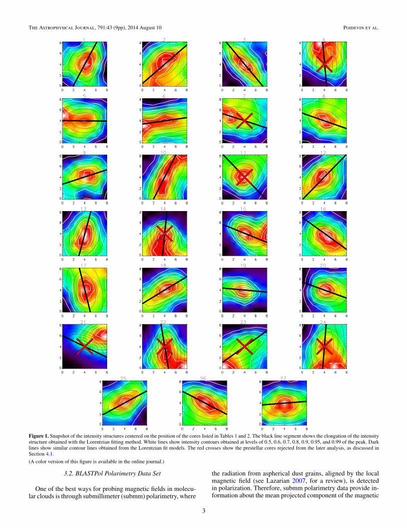
Figure 1. Snapshot of the intensity structures centered on the position of the cores listed in Tables 1 and 2. The black line segment shows the elongation of the intensitystructure obtained with the Lorentzian fitting method. White lines show intensity contours obtained at levels of 0.5, 0.6, 0.7, 0.8, 0.9, 0.95, and 0.99 of the peak. Darklines show similar contour lines obtained from the Lorentzian fit models. The red crosses show the prestellar cores rejected from the later analysis, as discussed inSection 4.1.

(A color version of this figure is available in the online journal.)

3.2. BLASTPol Polarimetry Data Set

One of the best ways for probing magnetic fields in molecu-lar clouds is through submillimeter (submm) polarimetry, where

the radiation from aspherical dust grains, aligned by the localmagnetic field (see Lazarian 2007, for a review), is detectedin polarization. Therefore, submm polarimetry data provide in-formation about the mean projected component of the magnetic

3

The Astrophysical Journal, 791:43 (9pp), 2014 August 10 Poidevin et al.

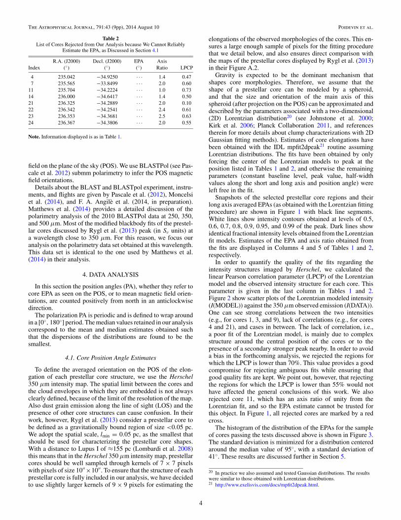
Table 2List of Cores Rejected from Our Analysis because We Cannot Reliably

Estimate the EPA, as Discussed in Section 4.1

R.A. (J2000) Decl. (J2000) EPA AxisIndex (◦) (◦) (◦) Ratio LPCP

4 235.042 −34.9250 · · · 1.4 0.477 235.565 −33.8499 · · · 2.0 0.60

11 235.704 −34.2224 · · · 1.0 0.7314 236.000 −34.6417 · · · 1.4 0.5021 236.325 −34.2889 · · · 2.0 0.1022 236.342 −34.2541 · · · 2.4 0.6123 236.353 −34.3681 · · · 2.5 0.6324 236.367 −34.3806 · · · 2.0 0.55

Note. Information displayed is as in Table 1.

field on the plane of the sky (POS). We use BLASTPol (see Pas-cale et al. 2012) submm polarimetry to infer the POS magneticfield orientations.

Details about the BLAST and BLASTpol experiment, instru-ments, and flights are given by Pascale et al. (2012), Moncelsiet al. (2014), and F. A. Angile et al. (2014, in preparation).Matthews et al. (2014) provides a detailed discussion of thepolarimetry analysis of the 2010 BLASTPol data at 250, 350,and 500 μm. Most of the modified blackbody fits of the prestel-lar cores discussed by Rygl et al. (2013) peak (in Sν units) ata wavelength close to 350 μm. For this reason, we focus ouranalysis on the polarimetry data set obtained at this wavelength.This data set is identical to the one used by Matthews et al.(2014) in their analysis.

4. DATA ANALYSIS

In this section the position angles (PA), whether they refer tocore EPA as seen on the POS, or to mean magnetic field orien-tations, are counted positively from north in an anticlockwisedirection.

The polarization PA is periodic and is defined to wrap aroundin a [0◦, 180◦] period. The median values retained in our analysiscorrespond to the mean and median estimates obtained suchthat the dispersions of the distributions are found to be thesmallest.

4.1. Core Position Angle Estimates

To define the averaged orientation on the POS of the elon-gation of each prestellar core structure, we use the Herschel350 μm intensity map. The spatial limit between the cores andthe cloud envelopes in which they are embedded is not alwaysclearly defined, because of the limit of the resolution of the map.Also dust grain emission along the line of sight (LOS) and thepresence of other core structures can cause confusion. In theirwork, however, Rygl et al. (2013) consider a prestellar core tobe defined as a gravitationally bound region of size <0.05 pc.We adopt the spatial scale, lmin = 0.05 pc, as the smallest thatshould be used for characterizing the prestellar core shapes.With a distance to Lupus I of ≈155 pc (Lombardi et al. 2008)this means that in the Herschel 350 μm intensity map, prestellarcores should be well sampled through kernels of 7 × 7 pixelswith pixels of size 10′′×10′′. To ensure that the structure of eachprestellar core is fully included in our analysis, we have decidedto use slightly larger kernels of 9 × 9 pixels for estimating the

elongations of the observed morphologies of the cores. This en-sures a large enough sample of pixels for the fitting procedurethat we detail below, and also ensures direct comparison withthe maps of the prestellar cores displayed by Rygl et al. (2013)in their Figure A.2.

Gravity is expected to be the dominant mechanism thatshapes core morphologies. Therefore, we assume that theshape of a prestellar core can be modeled by a spheroid,and that the size and orientation of the main axis of thisspheroid (after projection on the POS) can be approximated anddescribed by the parameters associated with a two-dimensional(2D) Lorentzian distribution20 (see Johnstone et al. 2000;Kirk et al. 2006; Planck Collaboration 2011, and referencestherein for more details about clump characterizations with 2DGaussian fitting methods). Estimates of core elongations havebeen obtained with the IDL mpfit2dpeak21 routine assumingLorentzian distributions. The fits have been obtained by onlyforcing the center of the Lorentzian models to peak at theposition listed in Tables 1 and 2, and otherwise the remainingparameters (constant baseline level, peak value, half-widthvalues along the short and long axis and position angle) wereleft free in the fit.

Snapshots of the selected prestellar core regions and theirlong axis averaged EPAs (as obtained with the Lorentzian fittingprocedure) are shown in Figure 1 with black line segments.White lines show intensity contours obtained at levels of 0.5,0.6, 0.7, 0.8, 0.9, 0.95, and 0.99 of the peak. Dark lines showidentical fractional intensity levels obtained from the Lorentzianfit models. Estimates of the EPA and axis ratio obtained fromthe fits are displayed in Columns 4 and 5 of Tables 1 and 2,respectively.

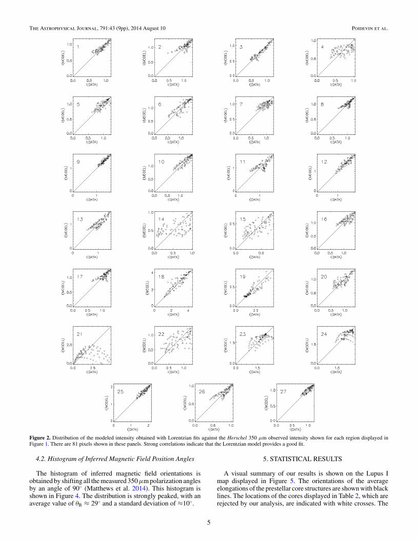
In order to quantify the quality of the fits regarding theintensity structures imaged by Herschel, we calculated thelinear Pearson correlation parameter (LPCP) of the Lorentzianmodel and the observed intensity structure for each core. Thisparameter is given in the last column in Tables 1 and 2.Figure 2 show scatter plots of the Lorentzian modeled intensity(I(MODEL)) against the 350 μm observed emission (I(DATA)).One can see strong correlations between the two intensities(e.g., for cores 1, 3, and 9), lack of correlations (e.g., for cores4 and 21), and cases in between. The lack of correlation, i.e.,a poor fit of the Lorentzian model, is mainly due to complexstructure around the central position of the cores or to thepresence of a secondary stronger peak nearby. In order to avoida bias in the forthcoming analysis, we rejected the regions forwhich the LPCP is lower than 70%. This value provides a goodcompromise for rejecting ambiguous fits while ensuring thatgood quality fits are kept. We point out, however, that rejectingthe regions for which the LPCP is lower than 55% would nothave affected the general conclusions of this work. We alsorejected core 11, which has an axis ratio of unity from theLorentzian fit, and so the EPA estimate cannot be trusted forthis object. In Figure 1, all rejected cores are marked by a redcross.

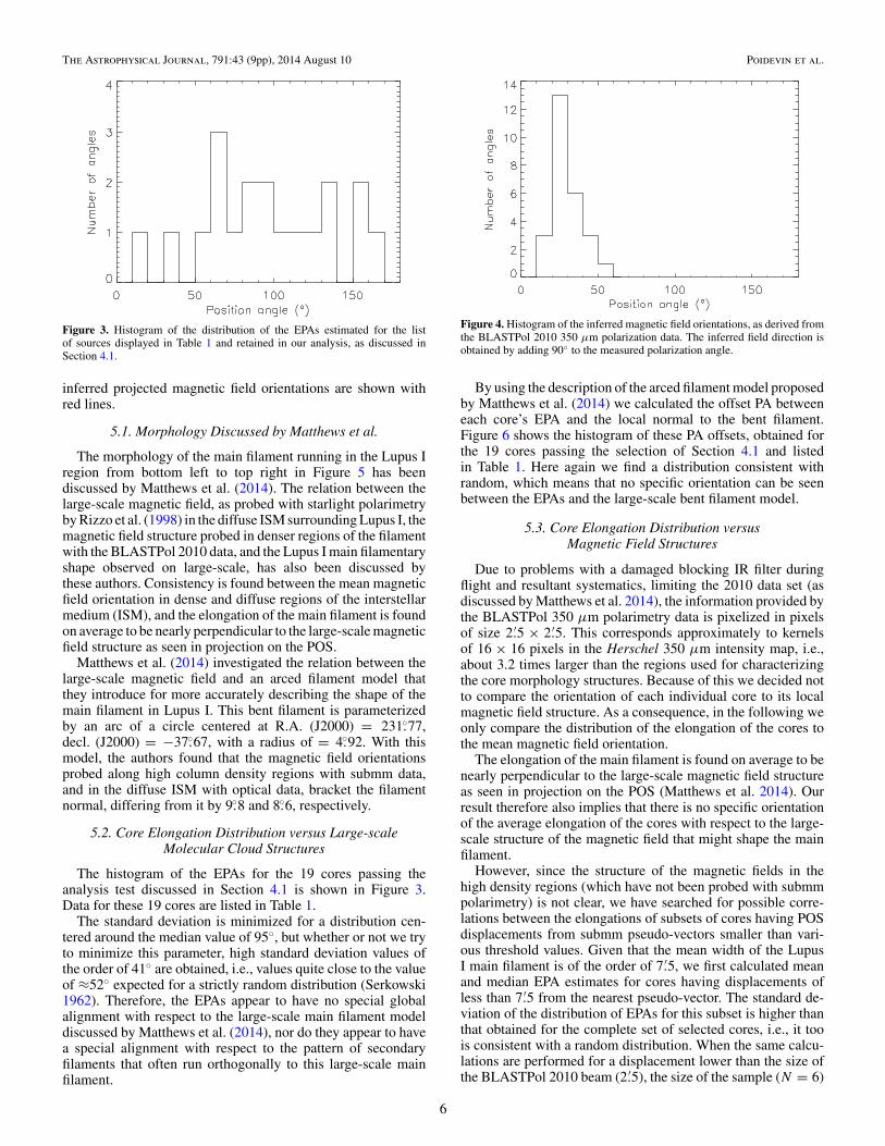
The histogram of the distribution of the EPAs for the sampleof cores passing the tests discussed above is shown in Figure 3.The standard deviation is minimized for a distribution centeredaround the median value of 95◦, with a standard deviation of41◦. These results are discussed further in Section 5.

20 In practice we also assumed and tested Gaussian distributions. The resultswere similar to those obtained with Lorentzian distributions.21 http://www.exelisvis.com/docs/mpfit2dpeak.html.

4

The Astrophysical Journal, 791:43 (9pp), 2014 August 10 Poidevin et al.

Figure 2. Distribution of the modeled intensity obtained with Lorentzian fits against the Herschel 350 μm observed intensity shown for each region displayed inFigure 1. There are 81 pixels shown in these panels. Strong correlations indicate that the Lorentzian model provides a good fit.

4.2. Histogram of Inferred Magnetic Field Position Angles

The histogram of inferred magnetic field orientations isobtained by shifting all the measured 350 μm polarization anglesby an angle of 90◦ (Matthews et al. 2014). This histogram isshown in Figure 4. The distribution is strongly peaked, with anaverage value of θB ≈ 29◦ and a standard deviation of ≈10◦.

5. STATISTICAL RESULTS

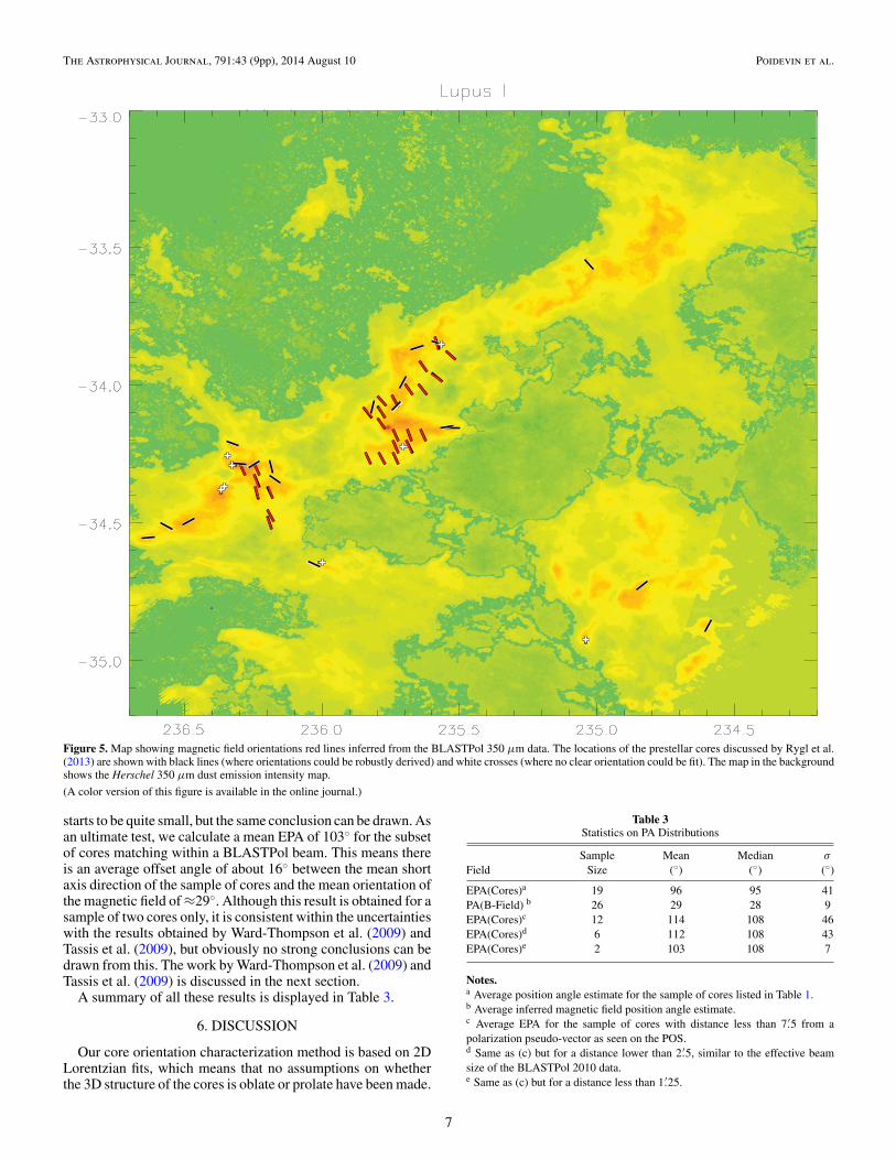
A visual summary of our results is shown on the Lupus Imap displayed in Figure 5. The orientations of the averageelongations of the prestellar core structures are shown with blacklines. The locations of the cores displayed in Table 2, which arerejected by our analysis, are indicated with white crosses. The

5

The Astrophysical Journal, 791:43 (9pp), 2014 August 10 Poidevin et al.

Figure 3. Histogram of the distribution of the EPAs estimated for the listof sources displayed in Table 1 and retained in our analysis, as discussed inSection 4.1.

inferred projected magnetic field orientations are shown withred lines.

5.1. Morphology Discussed by Matthews et al.

The morphology of the main filament running in the Lupus Iregion from bottom left to top right in Figure 5 has beendiscussed by Matthews et al. (2014). The relation between thelarge-scale magnetic field, as probed with starlight polarimetryby Rizzo et al. (1998) in the diffuse ISM surrounding Lupus I, themagnetic field structure probed in denser regions of the filamentwith the BLASTPol 2010 data, and the Lupus I main filamentaryshape observed on large-scale, has also been discussed bythese authors. Consistency is found between the mean magneticfield orientation in dense and diffuse regions of the interstellarmedium (ISM), and the elongation of the main filament is foundon average to be nearly perpendicular to the large-scale magneticfield structure as seen in projection on the POS.

Matthews et al. (2014) investigated the relation between thelarge-scale magnetic field and an arced filament model thatthey introduce for more accurately describing the shape of themain filament in Lupus I. This bent filament is parameterizedby an arc of a circle centered at R.A. (J2000) = 231.◦77,decl. (J2000) = −37.◦67, with a radius of = 4.◦92. With thismodel, the authors found that the magnetic field orientationsprobed along high column density regions with submm data,and in the diffuse ISM with optical data, bracket the filamentnormal, differing from it by 9.◦8 and 8.◦6, respectively.

5.2. Core Elongation Distribution versus Large-scaleMolecular Cloud Structures

The histogram of the EPAs for the 19 cores passing theanalysis test discussed in Section 4.1 is shown in Figure 3.Data for these 19 cores are listed in Table 1.

The standard deviation is minimized for a distribution cen-tered around the median value of 95◦, but whether or not we tryto minimize this parameter, high standard deviation values ofthe order of 41◦ are obtained, i.e., values quite close to the valueof ≈52◦ expected for a strictly random distribution (Serkowski1962). Therefore, the EPAs appear to have no special globalalignment with respect to the large-scale main filament modeldiscussed by Matthews et al. (2014), nor do they appear to havea special alignment with respect to the pattern of secondaryfilaments that often run orthogonally to this large-scale mainfilament.

Figure 4. Histogram of the inferred magnetic field orientations, as derived fromthe BLASTPol 2010 350 μm polarization data. The inferred field direction isobtained by adding 90◦ to the measured polarization angle.

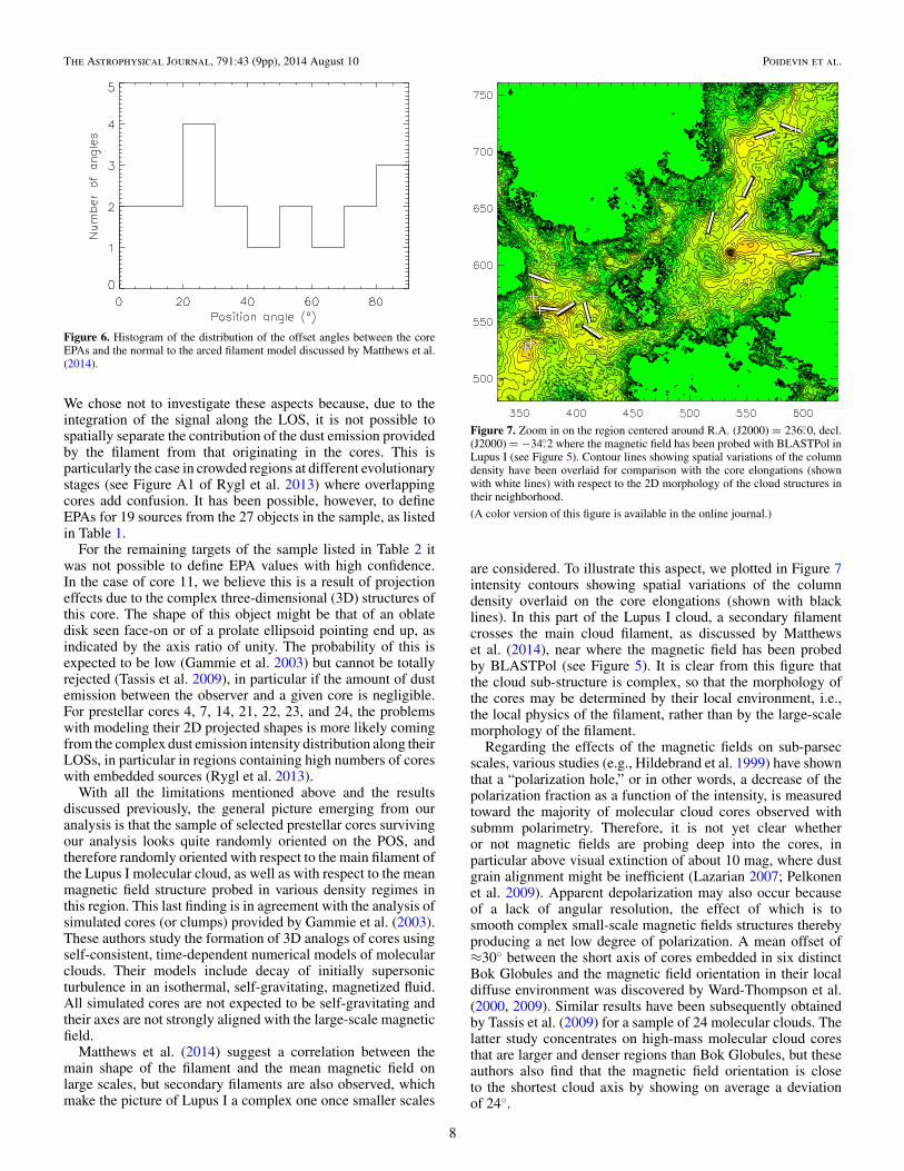
By using the description of the arced filament model proposedby Matthews et al. (2014) we calculated the offset PA betweeneach core’s EPA and the local normal to the bent filament.Figure 6 shows the histogram of these PA offsets, obtained forthe 19 cores passing the selection of Section 4.1 and listedin Table 1. Here again we find a distribution consistent withrandom, which means that no specific orientation can be seenbetween the EPAs and the large-scale bent filament model.

5.3. Core Elongation Distribution versusMagnetic Field Structures

Due to problems with a damaged blocking IR filter duringflight and resultant systematics, limiting the 2010 data set (asdiscussed by Matthews et al. 2014), the information provided bythe BLASTPol 350 μm polarimetry data is pixelized in pixelsof size 2.′5 × 2.′5. This corresponds approximately to kernelsof 16 × 16 pixels in the Herschel 350 μm intensity map, i.e.,about 3.2 times larger than the regions used for characterizingthe core morphology structures. Because of this we decided notto compare the orientation of each individual core to its localmagnetic field structure. As a consequence, in the following weonly compare the distribution of the elongation of the cores tothe mean magnetic field orientation.

The elongation of the main filament is found on average to benearly perpendicular to the large-scale magnetic field structureas seen in projection on the POS (Matthews et al. 2014). Ourresult therefore also implies that there is no specific orientationof the average elongation of the cores with respect to the large-scale structure of the magnetic field that might shape the mainfilament.

However, since the structure of the magnetic fields in thehigh density regions (which have not been probed with submmpolarimetry) is not clear, we have searched for possible corre-lations between the elongations of subsets of cores having POSdisplacements from submm pseudo-vectors smaller than vari-ous threshold values. Given that the mean width of the LupusI main filament is of the order of 7.′5, we first calculated meanand median EPA estimates for cores having displacements ofless than 7.′5 from the nearest pseudo-vector. The standard de-viation of the distribution of EPAs for this subset is higher thanthat obtained for the complete set of selected cores, i.e., it toois consistent with a random distribution. When the same calcu-lations are performed for a displacement lower than the size ofthe BLASTPol 2010 beam (2.′5), the size of the sample (N = 6)

6

The Astrophysical Journal, 791:43 (9pp), 2014 August 10 Poidevin et al.

Figure 5. Map showing magnetic field orientations red lines inferred from the BLASTPol 350 μm data. The locations of the prestellar cores discussed by Rygl et al.(2013) are shown with black lines (where orientations could be robustly derived) and white crosses (where no clear orientation could be fit). The map in the backgroundshows the Herschel 350 μm dust emission intensity map.

(A color version of this figure is available in the online journal.)

starts to be quite small, but the same conclusion can be drawn. Asan ultimate test, we calculate a mean EPA of 103◦ for the subsetof cores matching within a BLASTPol beam. This means thereis an average offset angle of about 16◦ between the mean shortaxis direction of the sample of cores and the mean orientation ofthe magnetic field of ≈29◦. Although this result is obtained for asample of two cores only, it is consistent within the uncertaintieswith the results obtained by Ward-Thompson et al. (2009) andTassis et al. (2009), but obviously no strong conclusions can bedrawn from this. The work by Ward-Thompson et al. (2009) andTassis et al. (2009) is discussed in the next section.

A summary of all these results is displayed in Table 3.

6. DISCUSSION

Our core orientation characterization method is based on 2DLorentzian fits, which means that no assumptions on whetherthe 3D structure of the cores is oblate or prolate have been made.

Table 3Statistics on PA Distributions

Sample Mean Median σ

Field Size (◦) (◦) (◦)

EPA(Cores)a 19 96 95 41PA(B-Field) b 26 29 28 9EPA(Cores)c 12 114 108 46EPA(Cores)d 6 112 108 43EPA(Cores)e 2 103 108 7

Notes.a Average position angle estimate for the sample of cores listed in Table 1.b Average inferred magnetic field position angle estimate.c Average EPA for the sample of cores with distance less than 7.′5 from apolarization pseudo-vector as seen on the POS.d Same as (c) but for a distance lower than 2.′5, similar to the effective beamsize of the BLASTPol 2010 data.e Same as (c) but for a distance less than 1.′25.

7

The Astrophysical Journal, 791:43 (9pp), 2014 August 10 Poidevin et al.

Figure 6. Histogram of the distribution of the offset angles between the coreEPAs and the normal to the arced filament model discussed by Matthews et al.(2014).

We chose not to investigate these aspects because, due to theintegration of the signal along the LOS, it is not possible tospatially separate the contribution of the dust emission providedby the filament from that originating in the cores. This isparticularly the case in crowded regions at different evolutionarystages (see Figure A1 of Rygl et al. 2013) where overlappingcores add confusion. It has been possible, however, to defineEPAs for 19 sources from the 27 objects in the sample, as listedin Table 1.

For the remaining targets of the sample listed in Table 2 itwas not possible to define EPA values with high confidence.In the case of core 11, we believe this is a result of projectioneffects due to the complex three-dimensional (3D) structures ofthis core. The shape of this object might be that of an oblatedisk seen face-on or of a prolate ellipsoid pointing end up, asindicated by the axis ratio of unity. The probability of this isexpected to be low (Gammie et al. 2003) but cannot be totallyrejected (Tassis et al. 2009), in particular if the amount of dustemission between the observer and a given core is negligible.For prestellar cores 4, 7, 14, 21, 22, 23, and 24, the problemswith modeling their 2D projected shapes is more likely comingfrom the complex dust emission intensity distribution along theirLOSs, in particular in regions containing high numbers of coreswith embedded sources (Rygl et al. 2013).

With all the limitations mentioned above and the resultsdiscussed previously, the general picture emerging from ouranalysis is that the sample of selected prestellar cores survivingour analysis looks quite randomly oriented on the POS, andtherefore randomly oriented with respect to the main filament ofthe Lupus I molecular cloud, as well as with respect to the meanmagnetic field structure probed in various density regimes inthis region. This last finding is in agreement with the analysis ofsimulated cores (or clumps) provided by Gammie et al. (2003).These authors study the formation of 3D analogs of cores usingself-consistent, time-dependent numerical models of molecularclouds. Their models include decay of initially supersonicturbulence in an isothermal, self-gravitating, magnetized fluid.All simulated cores are not expected to be self-gravitating andtheir axes are not strongly aligned with the large-scale magneticfield.

Matthews et al. (2014) suggest a correlation between themain shape of the filament and the mean magnetic field onlarge scales, but secondary filaments are also observed, whichmake the picture of Lupus I a complex one once smaller scales

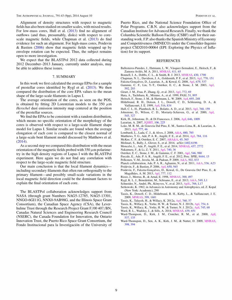
Figure 7. Zoom in on the region centered around R.A. (J2000) = 236.◦0, decl.(J2000) = −34.◦2 where the magnetic field has been probed with BLASTPol inLupus I (see Figure 5). Contour lines showing spatial variations of the columndensity have been overlaid for comparison with the core elongations (shownwith white lines) with respect to the 2D morphology of the cloud structures intheir neighborhood.

(A color version of this figure is available in the online journal.)

are considered. To illustrate this aspect, we plotted in Figure 7intensity contours showing spatial variations of the columndensity overlaid on the core elongations (shown with blacklines). In this part of the Lupus I cloud, a secondary filamentcrosses the main cloud filament, as discussed by Matthewset al. (2014), near where the magnetic field has been probedby BLASTPol (see Figure 5). It is clear from this figure thatthe cloud sub-structure is complex, so that the morphology ofthe cores may be determined by their local environment, i.e.,the local physics of the filament, rather than by the large-scalemorphology of the filament.

Regarding the effects of the magnetic fields on sub-parsecscales, various studies (e.g., Hildebrand et al. 1999) have shownthat a “polarization hole,” or in other words, a decrease of thepolarization fraction as a function of the intensity, is measuredtoward the majority of molecular cloud cores observed withsubmm polarimetry. Therefore, it is not yet clear whetheror not magnetic fields are probing deep into the cores, inparticular above visual extinction of about 10 mag, where dustgrain alignment might be inefficient (Lazarian 2007; Pelkonenet al. 2009). Apparent depolarization may also occur becauseof a lack of angular resolution, the effect of which is tosmooth complex small-scale magnetic fields structures therebyproducing a net low degree of polarization. A mean offset of≈30◦ between the short axis of cores embedded in six distinctBok Globules and the magnetic field orientation in their localdiffuse environment was discovered by Ward-Thompson et al.(2000, 2009). Similar results have been subsequently obtainedby Tassis et al. (2009) for a sample of 24 molecular clouds. Thelatter study concentrates on high-mass molecular cloud coresthat are larger and denser regions than Bok Globules, but theseauthors also find that the magnetic field orientation is closeto the shortest cloud axis by showing on average a deviationof 24◦.

8

The Astrophysical Journal, 791:43 (9pp), 2014 August 10 Poidevin et al.

Alignment of density structures with respect to magneticfields has also been studied on smaller scales, with mixed results.For low-mass cores, Hull et al. (2013) find no alignment ofoutflows (and thus, presumably, disks) with respect to core-scale magnetic fields, while Chapman et al. (2013) do findevidence for such an alignment. For high-mass cores, Poidevin& Bastien (2006) show that magnetic fields wrapped up byenvelope rotation can be expected. Thus, the subject remainsopen to more investigation.

We expect that the BLASTPol 2012 data collected during2012 December–2013 January, currently under analysis, maybe able to address these issues.

7. SUMMARY

In this work we first calculated the average EPAs for a sampleof prestellar cores identified by Rygl et al. (2013). We thencompared the distribution of the core EPA values to the meanshape of the large-scale filaments in Lupus I.

The average orientation of the cores, as seen on the POS,is obtained by fitting 2D Lorentzian models to the 350 μmHerschel dust emission intensity map centered at the positionof the prestellar sources.

We find the EPAs to be consistent with a random distribution,which means no specific orientation of the morphology of thecores is observed with respect to a large-scale filament shapemodel for Lupus I. Similar results are found when the averageelongation of each core is compared to the closest normal ofa large-scale bent filament model discussed by Matthews et al.(2014).

As a second step we compared this distribution with the meanorientation of the magnetic fields probed with 350 μm polarime-try in the high density regions of Lupus I with the BLASTPolexperiment. Here again we do not find any correlation withrespect to the large-scale magnetic field structure.

Our main conclusion is that the local filament dynamics—including secondary filaments that often run orthogonally to theprimary filament—and possibly small-scale variations in thelocal magnetic field direction could be the dominant factors toexplain the final orientation of each core.

The BLASTPol collaboration acknowledges support fromNASA (through grant Numbers NAG5-12785, NAG5-13301,NNGO-6GI11G, NNX0-9AB98G, and the Illinois Space GrantConsortium), the Canadian Space Agency (CSA), the Lever-hulme Trust through the Research Project Grant F/00 407/BN,Canadas Natural Sciences and Engineering Research Council(NSERC), the Canada Foundation for Innovation, the OntarioInnovation Trust, the Puerto Rico Space Grant Consortium, theFondo Institucional para la Investigacion of the University of

Puerto Rico, and the National Science Foundation Office ofPolar Programs. C.B.N. also acknowledges support from theCanadian Institute for Advanced Research. Finally, we thank theColumbia Scientific Balloon Facility (CSBF) staff for their out-standing work. F.P. also thanks the Spanish Ministry of Economyand Competitiveness (MINECO) under the Consolider-Ingenioproject CSD2010-00064 (EPI: Exploring the Physics of Infla-tion) for its support.

REFERENCES

Ballesteros-Paredes, J., Hatmann, L. W., Vasquez-Semadeni, E., Heitsch, F., &Zamora-Aviles, M. A. 2011, MNRAS, 411, 65

Bonnell, I. A., Dobbs, C. L., & Smith, R. J. 2013, MNRAS, 430, 1790Chapman, N. L., Davidson, J. A., Goldsmith, P. F., et al. 2013, ApJ, 770, 151Falceta-Goncalves, D., Lazarian, A., & Kowal, G. 2008, ApJ, 679, 537Gammie, C. F., Lin, Y.-T., Ostriker, E. C., & Stone, J. M. 2003, ApJ,

592, 203Girart, J. M., Frau, P., Zhang, Q., et al. 2013, ApJ, 772, 69Hara, A., Tachihara, K., Mizuno, A., et al. 1999, PASJ, 51, 895Heitsch, F., Stone, J. M., & Hartmann, L. W. 2009, ApJ, 695, 248Hildebrand, R. H., Dotson, J. L., Dowell, C. D., Schleuning, D. A., &

Vaillancourt, J. E. 1999, ApJ, 516, 834Hull, C. L. H., Plambeck, R. L., Bolatto, A. D., et al. 2013, ApJ, 768, 159Johnstone, D., Wilson, C. D., Moriarty-Schieven, G., et al. 2000, ApJ,

545, 327Kirk, H., Johnstone, D., & Di Francesco, J. 2006, ApJ, 646, 1009Lazarian, A. 2007, JQSRT, 106, 225Leao, M. R. M., de Gouveia Dal Pino, E. M., Santos-Lima, R., & Lazarian, A.

2013, ApJ, 777, 46Lombardi, L., Lada, C. J., & Alves, J. 2008, A&A, 480, 785Matthews, T. G., Ade, P. A. R., Angile, F. E., et al. 2014, ApJ, 784, 116McKee, C. F., & Ostriker, E. C. 2007, ARA&A, 45, 565Molinari, S., Bally, J., Glover, S., et al. 2014, arXiv:1402.6196Moncelsi, L., Ade, P., Angile, F. E., et al. 2014, MNRAS, 437, 2772Nakamura, F., & Li, Z.-Y. 2011, ApJ, 740, 36Ostriker, E. C., Stone, J. M., & Gammie, C. F. 2001, ApJ, 546, 980Pascale, E., Ade, P. A. R., Angile, F. E., et al. 2012, Proc. SPIE, 8444, 15Pelkonen, V.-M., Juvela, M., & Padoan, P. 2009, A&A, 502, 833Planck collaboration, Ade, P. A. R., Aghanim, N., et al. 2011, A&A, 536, A23Poidevin, F., & Bastien, P. 2006, ApJ, 650, 945Poidevin, F., Falceta-Goncalves, D., Kowal, G., De Gouveia Del Pino, E., &

Magalhaes, A. M. 2013, ApJ, 777, 112Rizzo, J., Morras, R., & Arnal, E. 1998, MNRAS, 300, 497Rygl, K. L. J., Benedettini, M., Schisano, E., et al. 2013, A&A, 549, L1Schneider, N., Andre, Ph., Konyves, V., et al. 2013, ApJL, 766, L17Serkowski, K. 1962, in Advances in Astronomy and Astrophysics, ed. Z. Kopal

(New York: Academic), 290Tassis, K., Dowell, C. D., Hildebrand, R. H., Kirby, L., & Vaillancourt, J. E.

2009, MNRAS, 399, 1681Tassis, K., Talayeh, H., & Willacy, K. 2012a, ApJ, 760, 57Tassis, K., Willacy, K., Yorke, H. W., & Turner, N. J. 2012b, ApJ, 754, 6Tassis, K., Willacy, K., Yorke, H. W., & Turner, N. J. 2012c, ApJ, 745, 68Ward, R. L., Wadsley, J., & Sills, A. 2014, MNRAS, 439, 651Ward-Thompson, D., Kirk, J. M., Crutcher, R. M., et al. 2000, ApJ,

537, 135Ward-Thomspon, D., Sen, A. K., Kirk, J. M., & Nutter, D. 2009, MNRAS,

398, 394

9