Page 1 of 19

Article DOI: http://dx.doi.org/10.3201/eid2401.1710851

Geogenomic Segregation and Temporal Trends of Human Pathogenic

Escherichia coli O157:H7

Technical Appendix 1

Supplementary Methods and Analyses

Assigning Phylogenetic Lineage to Non–SNP-Typed Isolates

In previous studies analyzing patterns associated with E. coli O157:H7 phylogenetic

classification, it has been common to use a single representative isolate from each PFGE subtype

(1–3). This practice masks the variability among isolates with the same PFGE fingerprint (e.g.,

variability in demographics, location). Further, estimation of effects at the population level is

compromised, because the isolates being analyzed are not reflective of the E. coli O157:H7 case

population distribution. To accurately make inference at the population level, we sought to

include all reported cases during the study period. Because we did not have sufficient resources

to SNP-type all isolates, we leveraged the assumption inherent in the single-representative-

isolate approach, although not generally made explicit: isolates with the same PFGE fingerprint

belong to the same phylogenetic grouping.

Our sample contained 1,160 isolates reflecting 355 unique XbaI PFGE patterns

(Technical Appendix Figure 1). We SNP-typed 793 of these isolates, covering 319 PFGE

subtypes. The 36 PFGE subtypes not SNP-typed were either biochemically atypical or they were

not present in the isolate bank. Atypical isolates were exclusively from 2013 and 2014, the last 2

years of sampling. Missing isolates were predominantly (82%) from 2005 and 2006, the first 2

years of sampling. Of the 793 SNP-typed isolates, 570 belonged to a PFGE subtype with

multiple SNP-typed isolates. Among these 570, we examined which phylogenetic lineages the

isolates had been assigned via SNP typing. All but 1 PFGE subtype were assigned a consistent

lineage. The one variable PFGE subtype was EXHX01.0047. It encompassed 82 isolates: 21

were not typed, 59 were typed to lineage IIa, and 2 were typed to lineage Ib. In other words, only

Page 2 of 19

2 of 570 isolates (0.4%) showed aberrant lineage assignment. With this, we felt that the

assumption that isolates of the same PFGE subtype would be in the same lineage held adequately

well to use the SNP-typing results to assign lineage to non–SNP-typed isolates. We were able to

assign lineage to 328 additional isolates by using this approach.

Spatial Segregation by Diggle’s Kernel Estimation Method

Diggle’s kernel estimation provides smoothed estimates of spatial segregation that take

into account multiple neighbors of each case. It provides an overall test of spatial segregation and

identifies statistically significant regions in the lineage-specific probability surfaces. Diggle’s

method assumes an underlying Poisson point process for each phylogenetic lineage. The degree

of smoothing is dependent on the choice of a bandwidth. A cross-validated log-likelihood

function can be used to calculate the bandwidth (4). We tested bandwidths between 0.02 and 1

degrees at 0.0098-degree increments to identify and then select for analysis the bandwidth

(0.6472 degrees) associated with the greatest cross-validated log-likelihood. Using the selected

bandwidth, we determined the lineage-specific probabilities based on the surrounding cases for

each case location and plotted the lineage-specific probability surfaces on individual maps. We

then calculated a test statistic for spatial segregation by summing the square of the difference

between the kernel regression-estimated lineage-specific probability at a given location and the

overall probability that a case isolate belongs to that lineage over all lineages and all case

locations. To determine statistical significance, we performed 999 Monte Carlo replications with

lineage randomly relabeled at each case location, maintaining the observed number of cases of

each lineage. The proportion of test statistics greater than that observed from the data was the p-

value. The analysis was conducted in R (5) using the spatialkernel package (6).

The bandwidth selected for the main analysis was used for all lineages within a given

analysis. To identify the sensitivity of the kernel estimation results to the bandwidth of 0.6472

degrees that was selected, alternate bandwidths were tested: 0.02, 0.1, 0.2, 0.4, and 0.9. All

yielded p = 0.001 for the overall test for spatial segregation. The segregation maps for individual

lineages grew predictably smoother as the bandwidth was increased and identified statistically

significant areas of segregation consistent with the primary result from a bandwidth of 0.6472.

Temporal variation in segregation was tested across 3 intervals: 2005–2007, 2008–2010,

and 2011–2014. The slightly longer last interval is not expected to affect the validity of the

Page 3 of 19

results. However, because of the greater number of cases in this interval, greater precision is

expected. We calculated a new bandwidth for each new analysis and subset of the data using the

cross-validated log-likelihood function. For the overall test of variation of spatial segregation

across time intervals using the kernel regression method, we chose a bandwidth of 0.8236

degrees. The bandwidths chosen for each of the individual intervals were 1.0000 for 2005–2007,

0.7256 for 2008–2010, and 0.9314 for 2011–2014. Not unexpectedly, given the high degree of

smoothing in the first and last periods, only the middle period had detectable overall spatial

segregation (p = 0.001). However, all periods displayed some statistically significant spatial

segregation for individual lineages (Technical Appendix Video). A bandwidth of 0.4 was also

tested for each of the intervals, resulting in statistically significant tests for overall spatial

segregation in each interval (2005–2007 p = 0.037, 2008–2010 p = 0.001, 2011–2014 p = 0.014).

Multinomial Generalized Additive Model

The multinomial GAM provides a smoothed risk surface relative to Ib, the most common

lineage. Unlike the direct measures of spatial segregation, the GAM captures spatial trends

without selecting a specific distance or number of neighbors across which to smooth. It does this

through a flexible spline function. The GAM also supports adjustment for covariates, providing

some assurance that the associations observed are not due to factors such as the distribution of

cases by age. The multinomial analysis entailed logistic-type equations for each of the 3 lineage

comparisons. Results of the GAM multinomial models must be interpreted conditional on having

a reported E. coli O157:H7 illness. As such, odds ratios presented estimate risk proportional to

that in the most common lineage, Ib.

We tested multiple aspects of the GAM specification. Latitude and longitude were

specified individually and jointly to allow interaction. The basis dimension of the penalized

regression smoother was altered to improve the effective degrees of freedom. Age and sex

covariates were removed, and the form of the spline smoother was altered. Lineage IIa was used

as the comparison lineage. These sensitivity analyses are summarized in Technical Appendix

Table 2. None of the model perturbations meaningfully changed the primary model results. In the

set of GAMs incorporating year, a trivariate smooth of latitude, longitude, and year was also

tested and found to be statistically significant for lineages IIa and IIb (Technical Appendix Table

2).

Page 4 of 19

Spatial Segregation by Dixon’s Nearest-Neighbor Method

Another measure of spatial segregation, Dixon’s nearest-neighbor method, considers only

the closest neighbor of each case. It conducts no smoothing and can be expected to be sensitive

to clustered outbreaks. This method does not indicate areas in which spatial segregation exists

but does provide an overall test of spatial segregation, as well as for segregation of individual

lineages and pairwise segregation tests. We created a 4 4 contingency table of nearest-neighbor

counts for each lineage group. A 2 test with 12 degrees of freedom was used to test overall

spatial segregation, and segregation was tested for each individual lineage group (Technical

Appendix Table 3). We calculated Dixon’s segregation index for each nearest-neighbor

combination (e.g., from Ib to IIa; Technical Appendix Table 4). Dixon’s pairwise segregation

index is defined as:

𝑆𝑖𝑗 = log𝑁𝑖𝑗/(𝑁𝑖 − 𝑁𝑖𝑗)

E𝑁𝑖𝑗/(𝑁𝑖 − E𝑁𝑖𝑗)= log

𝑁𝑖𝑗/(𝑁𝑖 − 𝑁𝑖𝑗)

𝑁𝑖/(𝑁 − 𝑁𝑗 − 1)

where i and j in this analysis are phylogenetic lineages (7). A positive value of S indicates

association, and a negative value indicates segregation. We calculated Z-scores for each

combination by comparing the observed nearest-neighbor count in each cell to the expected

count. We calculated a p-value based on the Z-scores assuming an asymptotic normal

distribution. We used the Dixon R package for this analysis (8).

We used Dixon 2 tests for segregation to indicate statistically significant segregation

overall (p < 0.001) and for lineages Ib (p = 0.046), IIa (p = 0.002), and IIb (p < 0.001), but not

for the group of clinically rare lineages (Technical Appendix Table 3). This is consistent with the

findings of the kernel estimation method, which found statistically significant overall spatial

segregation and identified areas of segregation for lineages Ib, IIa, and IIb. Dixon’s method also

tests associations between individual lineages. Pairwise nearest-neighbor comparisons showed

statistically significant positive association from each of lineages Ib, IIa, and IIb to itself.

Segregation was observed from Ib to IIa, IIa to the rare lineages, IIb to all other lineages, and the

rare lineages to Ib (Technical Appendix Table 4).

We examined spatial segregation with Dixon’s method for the 3 intervals analyzed with

the kernel estimation method. Spatial segregation was found to be statistically significant with p

< 0.001 during all 3 periods, contrasting with Diggle’s method, which identified statistically

Page 5 of 19

significant overall segregation only during the 2008–2010 period. However, the 2 spatial

segregation tests were consistent in identifying spatial segregation of lineage IIb during all

intervals (p < 0.001 for Dixon’s method during all intervals). Additionally, Dixon’s method

identified segregation of lineage IIa during the 2005–2007 period (p < 0.001) and segregation of

lineage Ib during the 2008–2010 (p < 0.001) and 2011–2014 (p = 0.005) periods.

Multinomial Spatial Scan Statistics

We used multinomial spatial scan statistics (9) in SaTScan (10) to identify clusters within

which the distribution of lineages differed significantly from the distribution of lineages outside

the cluster. The spatial scan statistics are designed to identify clusters of disease. In the

multinomial framework used here, the clusters reflect areas within which the distribution of cases

by lineage is skewed compared with the area outside the cluster. These are similar to the areas of

segregation identified by the kernel regression method. However, the scan statistics look at the

distribution of all 4 lineages simultaneously and not individually, thus allowing detection of

clusters in which multiple lineages may be out of proportion. Like the multinomial GAM

models, the multinomial spatial scan statistics must be interpreted conditionally on having a

reported E. coli O157:H7 illness.

For the primary spatial scan statistic model, we used a maximum cluster size of 20% of

cases. Statistical significance of the clusters was determined based on Monte Carlo replications

under the null. Relative risks presented estimate risk of one’s infection being from the given

lineage inside the cluster compared with the risk outside that cluster.

We identified 3 statistically significant clusters in which the distribution of cases by

phylogenetic lineage varied from the distribution in the rest of the state (Technical Appendix

Figure 2). The first cluster (p = 0.001) contained 203 cases, was centered in the southwest region

of the state, and was characterized by a higher proportion of lineage IIb cases than observed

elsewhere in the state (relative risk [RR] 2.59). The second cluster (p = 0.001), encompassing the

sparsely populated northern reaches of the state, contained 185 cases and had somewhat more Ib

(RR 1.37) and rare lineage (RR 1.88) cases and fewer IIb cases (RR 0.29). The final significant

cluster (p = 0.006) contained 79 cases in the south-central region of the state; lineage IIa was

more common than elsewhere in the state (RR 1.70), IIb was uncommon (RR 0.13), and cases

due to rare lineages were nearly absent (RR 0). The first cluster, dominated by IIb, and third

Page 6 of 19

cluster, dominated by IIa, recapitulate the results of the kernel estimation maps and, for IIb, the

GAM-generated risk surface. The second cluster, dominated by lineage Ib, is larger and centered

somewhat further east than the area of segregation identified for Ib by the kernel estimation

method, though still similar.

Altering the parameters of the analysis to allow lower or higher percentages of the cases

to be included in clusters did not meaningfully affect the position of the clusters identified. We

tested allowing clusters up to 50% of cases and 10% of cases. From the former, the main IIb-

dominant and Ib/rare-dominant clusters were identified, but the IIa-dominated cluster was not.

Limiting clusters to 10% of cases, all 3 clusters identified in the primary analysis were identified

but with smaller numbers of included cases.

We detected variant clusters using multinomial spatiotemporal scan statistics, using year

as the time scale and allowing up to 50% of the study period in a cluster, as well as purely spatial

clusters. We identified 3 statistically significant clusters (Technical Appendix Figure 3). The first

(p = 0.001) contained 76 cases reported during 2009–2012 in the southwest region of the state

and had an elevated risk of lineage IIb (RR 4.45). The second cluster (p = 0.001) included 107

cases across the northeast region during 2005–2009. The Ib (RR 1.61) and rare (RR 1.88)

lineages were elevated. The third cluster (p = 0.002) included only 46 cases reported during

2009–2010, with a predominance of lineage IIb (RR 3.63) and near-absence of IIa (RR 0.09).

This cluster included part of Seattle, Washington’s largest urban area, and areas immediately

south and east.

Secondary Cases

To separate the effect of person-to-person transmission from other potential

environmental factors that may result in segregation, we conducted sensitivity analyses after

excluding known secondary cases. To be excluded, the most likely source of the infection had to

have been identified during the public health investigation as person-to-person, or the notes had

to indicate that another individual in the household or childcare situation had previously received

such a diagnosis. Based on these criteria, 82 secondary cases were excluded. No meaningful

changes in the results were observed. The overall test of spatial segregation was statistically

significant using the kernel estimation method (p = 0.002) and the nearest-neighbor method (p <

0.001). The latitude/longitude smooth of lineage IIb from the multinomial GAM is statistically

Page 7 of 19

significantly different from that of lineage Ib (p < 0.001). However, the cluster identified in the

southwest region of the state, dominated by lineage IIb, through multinomial spatial scan

statistics moved somewhat northward and decreased in size without the secondary cases.

Reporting Bias

We assessed potential reporting bias by county. Reporting of patients who have tested

positive is considered near 100% (11), but testing intensity may vary by provider. E. coli

O157:H7 is most often detected by fecal specimen culture, a test that also detects

Campylobacter, Salmonella, and Shigella. If providers in an area have heightened awareness of

E. coli O157:H7 and are more likely to test for it than in other areas, we would expect that

detection of these other pathogens would also be higher. There is overlap in the epidemiology of

E. coli O157:H7, Campylobacter, and Salmonella, so some correlation is expected. However,

risk factors for Shigella are generally different (12). If there were reporting bias, we would

expect this to have the greatest impact on the observed incidence of milder E. coli O157:H7

strains.

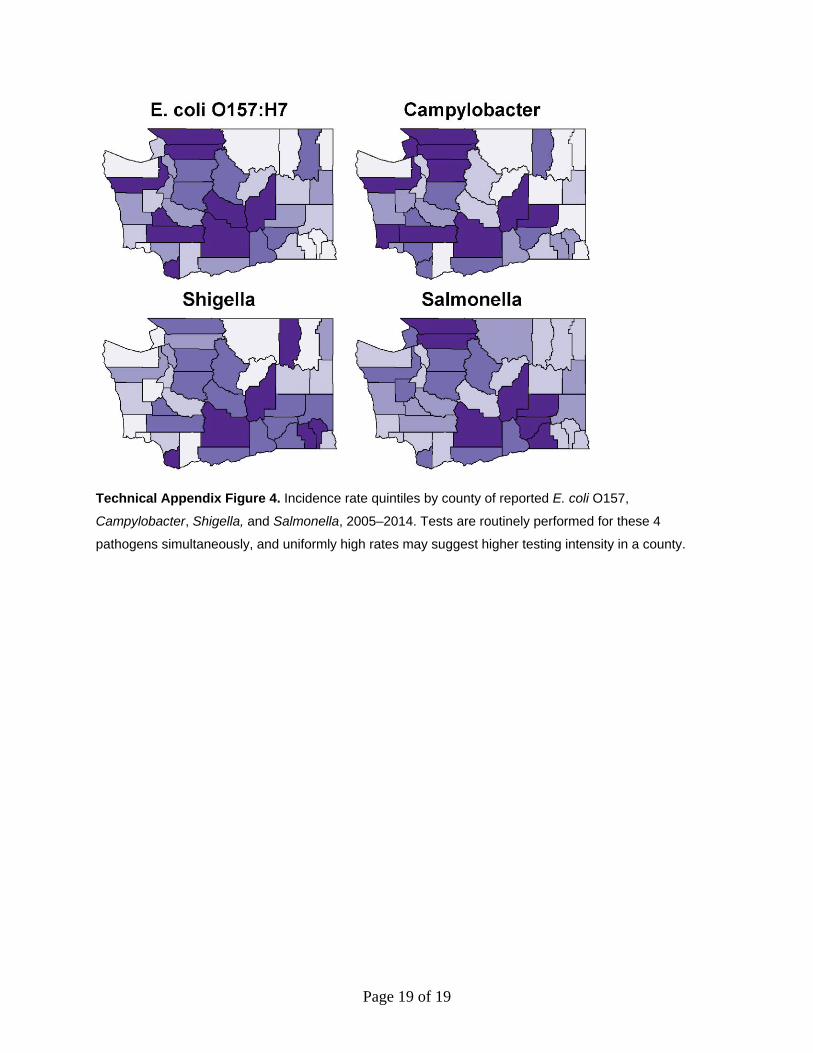
Case counts by county for 2005–2014 for campylobacteriosis, salmonellosis, and

shigellosis were obtained from the Washington State Communicable Disease Reports for 2009

and 2014 (each contained 5 years of data) (13,14). We calculated incidence rates using county

populations as reported in 2010 U.S. Census TIGER/Line Shapefiles (15). Using the GISTools

(16) package in R, we mapped the incidence quintile of each of the 4 pathogens at the county

level for the study period to assess the potential for reporting bias (Technical Appendix Figure

4). Two counties, Yakima and Grant, appear in the uppermost quintile of incidence for each of

the 4 diseases. However, incidence of rare lineage E. coli O157:H7 in this region is remarkably

low (main article Figure 1; Technical Appendix Figure 2). Infections caused by these bacteria are

generally milder (main article Table) and would be the type whose numbers would be

exaggerated in the presence of heightened testing. Thus, it is unlikely that reporting bias is

responsible for the observed results.

Data

Genomic data, with limited metadata, on all isolates used in the study are provided in

Technical Appendix 2 (https://wwwnc.cdc.gov/EID/article/23/1/17-0851-Techapp2.xlsx). These

include genomic data on all 1,160 E. coli O157:H7 isolates from reported, culture-confirmed

Page 8 of 19

cases in Washington state, 2005–2014. Phylogenetic lineage was determined directly using the

48-plex SNP assay developed by Jung et al. (17) or was inferred from a typed isolate with the

same PFGE profile. Shiga toxin bacteriophage insertion typing and typing for clade according to

the method used by Manning et al. (2) were conducted on only a subset of isolates. NT, not

typed; PFGE, pulsed field gel electrophoresis; SBI, Shiga toxin bacteriophage insertion typing;

SDM, Shannon Manning clade/genotype.

References

1. Iyoda S, Manning SD, Seto K, Kimata K, Isobe J, Etoh Y, et al. Phylogenetic clades 6 and 8 of

enterohemorrhagic Escherichia coli O157:H7 with particular stx subtypes are more frequently

found in isolates from hemolytic uremic syndrome patients than from asymptomatic carriers.

Open Forum Infect Dis. 2014;1:ofu061. http://dx.doi.org/10.1093/ofid/ofu061

2. Manning SD, Motiwala AS, Springman AC, Qi W, Lacher DW, Ouellette LM, et al. Variation in

virulence among clades of Escherichia coli O157:H7 associated with disease outbreaks. Proc Natl

Acad Sci U S A. 2008;105:4868–73. http://dx.doi.org/10.1073/pnas.0710834105

3. Pianciola L, Chinen I, Mazzeo M, Miliwebsky E, González G, Müller C, et al. Genotypic

characterization of Escherichia coli O157:H7 strains that cause diarrhea and hemolytic uremic

syndrome in Neuquén, Argentina. Int J Med Microbiol. 2014;304:499–504.

http://dx.doi.org/10.1016/j.ijmm.2014.02.011

4. Diggle PJ, Zheng P, Durr P. Nonparametric estimation of spatial segregation in a multivariate point

process: bovine tuberculosis in Cornwall, UK. Appl Stat. 2005;54:645–58.

http://dx.doi.org/10.1111/j.1467-9876.2005.05373.x

5. R Core Team. R: a language and environment for statistical computing. Vienna: R Foundation for

Statistical Computing; 2015.

6. Zheng P, Diggle PJ. Spatialkernel: nonparametric estimation of spatial segregation in a multivariate

point process; R package version 0.4-19. 2013 [cited 2015 May 27]. https://CRAN.R-

project.org/package=spatialkernel

7. Dixon PM. Nearest-neighbor contingency table analysis of spatial segregation for several species.

Écoscience. 2002;9:142–51. http://dx.doi.org/10.1080/11956860.2002.11682700

Page 9 of 19

8. de la Cruz M. Metodos Para Analizar Datos Puntuales. In: Maestre, FT, Escudero, A, Bonet, A, editors.

Introduccion Al Analisis Espacial De Datos En Ecologia Y Ciencias Ambientales: Metodos Y

Aplicaciones. Madrid: Asociacion Espanola de Ecologia Terrestre, Universidad Rey Juan Carlos

and Caja de Ahorros del Mediterraneo; 2008. p. 76–127.

9. Jung I, Kulldorff M, Richard OJ. A spatial scan statistic for multinomial data. Stat Med. 2010;29:1910–

8. http://dx.doi.org/10.1002/sim.3951

10. Kulldorff M, Information Management Services I. Satscantm V8.0: Software for the spatial and space-

time scan statistics. 2009 [cited 2015 May 27]. http://www.satscan.org/

11. Scallan E, Hoekstra RM, Angulo FJ, Tauxe RV, Widdowson MA, Roy SL, et al. Foodborne illness

acquired in the United States—major pathogens. Emerg Infect Dis. 2011;17:7–15.

http://dx.doi.org/10.3201/eid1701.P11101

12. Denno DM, Keene WE, Hutter CM, Koepsell JK, Patnode M, Flodin-Hursh D, et al. Tri-county

comprehensive assessment of risk factors for sporadic reportable bacterial enteric infection in

children. J Infect Dis. 2009;199:467–76. http://dx.doi.org/10.1086/596555

13. Communicable Disease Epidemiology Section. Communicable Disease Report 2014. Shoreline, WA:

Washington State Department of Health; 2014. p. 95.

14. Communicable Disease Epidemiology Section. Communicable Disease Report 2009. Shoreline, WA:

Washington State Department of Health; 2009. p. 91.

15. United States Census Bureau. 2012 Tiger/Line Shapefiles (Machine-Readable Data Files).

Washington, DC: The Bureau; 2012.

16. Brundsdon C, Chen H. GIStools: some further GIS capabilities for R; R package version 0.7-4. 2014

[cited 2015 May 27]. https://CRAN.R-project.org/package=GISTools

17. Jung WK, Bono JL, Clawson ML, Leopold SR, Shringi S, Besser TE. Lineage and genogroup-

defining single nucleotide polymorphisms of Escherichia coli O157:H7. Appl Environ Microbiol.

2013;79:7036–41. http://dx.doi.org/10.1128/AEM.02173-13

Page 10 of 19

Technical Appendix Table 1. Association of known risk factors with phylogenetic lineage*

Variable Statewide frequency

Statewide OR (95% CI)

Southwest region (n = 234)

OR (95% CI)

Northwest region (n = 289)

OR (95% CI)

South-central region (n = 109)

OR (95% CI)

Hispanic ethnicity (vs. non-Hispanic) Lineage Ib 46/372 Ref Ref Ref Ref Lineage IIa 32/197 1.13 (0.67, 1.91) 0.3 (0.03, 2.86) 2.79 (0.66, 11.83) 0.87 (0.33, 2.25) Lineage IIb 19/152 1.13 (0.61, 2.11) 0.99 (0.3, 3.33) 3.24 (0.62, 16.86) 0.73 (0.12, 4.37) Rare lineage 6/42 1.21 (0.46, 3.15) 8.15 (0.89, 75.06) 1.98 (0.18, 21.31) 0 (0, Inf)† American Indian (vs. white race)‡ Lineage Ib 5/377 Ref Ref Ref Ref Lineage IIa 7/196 3.82 (1.13, 12.95)§ NA NA NA Lineage IIb 0/148 0 (0, Inf)† NA NA NA Rare lineage 0/40 0 (0, Inf)† NA NA NA Asian race (vs. white race)‡ Lineage Ib 24/377 Ref Ref Ref Ref Lineage IIa 7/196 0.53 (0.22, 1.28) NA NA NA Lineage IIb 19/148 2.03 (1.02, 4.01)§ NA NA NA Rare lineage 2/40 0.72 (0.16, 3.22) NA NA NA Black race (vs. white race)‡ Lineage Ib 12/377 Ref Ref Ref Ref Lineage IIa 5/196 0.81 (0.27, 2.43) NA NA NA Lineage IIb 5/148 1.02 (0.34, 3.06) NA NA NA Rare lineage 0/40 0 (0, Inf)† NA NA NA Other/multiple race (vs. white race)‡ Lineage Ib 16/377 Ref Ref Ref Ref Lineage IIa 9/196 0.94 (0.39, 2.23) NA NA NA Lineage IIb 11/148 1.59 (0.69, 3.68) NA NA NA Rare lineage 1/40 0.55 (0.07, 4.32) NA NA NA Contact with a laboratory-confirmed case Lineage Ib 59/531 Ref Ref Ref Ref Lineage IIa 39/228 1.34 (0.84, 2.15) 0.88 (0.3, 2.6) 1.48 (0.63, 3.49) 0.99 (0.25, 3.96) Lineage IIb 43/176 1.96 (1.21, 3.16)¶ 2.7 (1.15, 6.31)§ 2.03 (0.78, 5.25) 2.74 (0.44, 17.21) Rare lineage 3/60 0.41 (0.12, 1.37) 0.42 (0.05, 3.82) 0.39 (0.05, 3.24) 0 (0, Inf)† Epidemiologic link to a confirmed or probable case Lineage Ib 74/522 Ref Ref Ref Ref Lineage IIa 41/221 1.25 (0.80, 1.96) 1.07 (0.37, 3.05) 0.97 (0.42, 2.25) 0.99 (0.24, 3.98) Lineage IIb 51/172 1.94 (1.24, 3.03)¶ 2.17 (0.94, 4.98) 1.41 (0.56, 3.55) 4.72 (0.85, 26.07) Rare lineage 3/60 0.32 (0.10, 1.06) 0.33 (0.04, 2.95) 0.29 (0.04, 2.39) 0 (0, Inf)† Underlying illness Lineage Ib 66/530 Ref Ref Ref Ref Lineage IIa 27/233 1.20 (0.70, 2.06) 2.87 (0.86, 9.61) 0.83 (0.2, 3.37) 4.07 (0.5, 33.02) Lineage IIb 19/184 1.11 (0.61, 2.01) 1.17 (0.36, 3.77) 0.73 (0.15, 3.59) 6.07 (0.33, 111.66) Rare lineage 2/62 0.19 (0.04, 0.85)§ 0.59 (0.06, 5.84) 0.42 (0.05, 3.73) 0 (0, Inf)† Contact with diapered or incontinent child or adult Lineage Ib 122/545 Ref Ref Ref Ref Lineage IIa 65/231 1.10 (0.75, 1.61) 0.91 (0.37, 2.22) 0.94 (0.42, 2.1) 1.43 (0.54, 3.79) Lineage IIb 60/187 1.28 (0.86, 1.91) 1.57 (0.76, 3.26) 1.58 (0.67, 3.73) 0.82 (0.13, 5.17) Rare lineage 8/62 0.53 (0.24, 1.16) 1.44 (0.36, 5.72) 0.19 (0.02, 1.52) 0.69 (0.06, 7.7) Attends childcare or preschool Lineage Ib 39/523 Ref Ref Ref Ref Lineage IIa 22/235 DNC 2.7 (0.68, 10.64) 1.7 (0.42, 6.86) 1.19 (0.21, 6.56) Lineage IIb 27/181 DNC 3.17 (1.03, 9.7)§ 2.16 (0.55, 8.57) 0 (0, Inf)† Rare lineage 0/59 DNC 0 (0, Inf)† 0 (0, Inf)† 0 (0, Inf)† Employed as a healthcare worker Lineage Ib 17/525 Ref Ref Ref Ref Lineage IIa 8/232 DNC 3.06 (0.44, 21.55) 0.7 (0.06, 8.42) 0 (0, Inf)† Lineage IIb 7/182 DNC 0.71 (0.06, 8.23) 1.52 (0.15, 15.38) 2.41 (0.18, 33.1) Rare lineage 1/62 DNC 0 (0, Inf)† 0 (0, Inf)† 0 (0, Inf)† Employed as a food worker Lineage Ib 18/539 Ref Ref Ref Ref Lineage IIa 12/244 1.64 (0.74, 3.59) 1.4 (0.1, 19.6) 1.58 (0.45, 5.56) 0 (0, Inf)† Lineage IIb 4/188 0.74 (0.24, 2.28) 1.61 (0.21, 12.62) 0.53 (0.06, 4.44) 0 (0, Inf)† Rare lineage 2/60 0.99 (0.22, 4.41) 0 (0, Inf)† 1.11 (0.13, 9.77) 0 (0, Inf)†

Page 11 of 19

Variable Statewide frequency

Statewide OR (95% CI)

Southwest region (n = 234)

OR (95% CI)

Northwest region (n = 289)

OR (95% CI)

South-central region (n = 109)

OR (95% CI) Works with animals or animal products Lineage Ib 24/524 Ref Ref Ref Ref Lineage IIa 5/196 0.46 (0.16, 1.27) 0 (0, Inf)† 0.31 (0.04, 2.57) 0.87 (0.12, 6.08) Lineage IIb 5/163 0.84 (0.30, 2.40) 0.77 (0.11, 5.45) 0 (0, Inf)† 2.17 (0.19, 24.56) Rare lineage 3/53 1.14 (0.33, 4.00) 2.87 (0.25, 33.45) 1.73 (0.32, 9.22) 0 (0, Inf)† Any contact with animals Lineage Ib 300/521 Ref Ref Ref Ref Lineage IIa 115/200 0.81 (0.57, 1.15) 0.84 (0.34, 2.09) 0.56 (0.26, 1.24) 0.48 (0.18, 1.3) Lineage IIb 90/167 0.78 (0.54, 1.14) 1.9 (0.89, 4.06) 0.48 (0.2, 1.15) 0.16 (0.03, 0.88)§ Rare lineage 27/52 0.8 (0.44, 1.45) Inf (0, Inf)† 0.73 (0.24, 2.26) 0.3 (0.02, 3.63) Contact with cattle, cows, or calves Lineage Ib 63/471 Ref Ref Ref Ref Lineage IIa 30/188 1.06 (0.64, 1.78) 1.11 (0.32, 3.81) 0.68 (0.26, 1.78) 1.06 (0.36, 3.12) Lineage IIb 13/151 0.59 (0.3, 1.14) 1.04 (0.38, 2.84) 0.14 (0.02, 1.07) 0 (0, Inf)† Rare lineage 7/49 1.19 (0.5, 2.81) 0.95 (0.1, 8.81) 0.92 (0.24, 3.54) 0 (0, Inf)† Case or household member lives or works on a farm or dairy Lineage Ib 67/526 Ref Ref Ref Ref Lineage IIa 24/191 0.86 (0.50, 1.46) 0.47 (0.09, 2.5) 0.96 (0.37, 2.44) 1.06 (0.36, 3.13) Lineage IIb 15/169 0.67 (0.35, 1.27) 1.62 (0.58, 4.48) 0 (0, Inf)† 0.33 (0.04, 2.95) Rare lineage 7/53 1.08 (0.47, 2.52) 1.35 (0.14, 13) 0.99 (0.26, 3.82) 1.39 (0.11, 17.56) Visited a zoo, farm, fair, or pet shop Lineage Ib 99/526 Ref Ref Ref Ref Lineage IIa 49/200 1.31 (0.86, 2) 1.59 (0.61, 4.17) 0.93 (0.41, 2.12) 1 (0.28, 3.53) Lineage IIb 25/166 0.59 (0.35, 1)§ 0.88 (0.4, 1.94) 0.17 (0.04, 0.78)§ 0 (0, Inf)† Rare lineage 11/53 1.11 (0.53, 2.33) 0.52 (0.06, 4.65) 0.6 (0.16, 2.32) 2.65 (0.2, 34.74) Recreational water exposure Lineage Ib 130/548 Ref Ref Ref Ref Lineage IIa 57/229 0.96 (0.65, 1.41) 0.51 (0.18, 1.45) 0.53 (0.24, 1.17) 0.79 (0.25, 2.56) Lineage IIb 38/174 0.82 (0.53, 1.27) 0.38 (0.16, 0.93)§ 0.44 (0.16, 1.24) 6.39 (1.09, 37.47)§ Rare lineage 12/60 0.79 (0.40, 1.57) 0.66 (0.13, 3.41) 0.77 (0.22, 2.73) 1.41 (0.12, 16.12) Drank untreated/unchlorinated water Lineage Ib 61/531 Ref Ref Ref Ref Lineage IIa 29/219 0.96 (0.58, 1.57) 4.49 (1.48, 13.57)¶ 0.89 (0.27, 2.87) 0.16 (0.04, 0.63)¶ Lineage IIb 26/169 1.27 (0.74, 2.16) 3.76 (1.38, 10.28)¶ 1.5 (0.44, 5.15) 0.27 (0.03, 2.38) Rare lineage 7/53 1.14 (0.49, 2.66) 1.68 (0.29, 9.69) 2.14 (0.41, 11.07) 0 (0, Inf)† Well is source of drinking water Lineage Ib 136/559 Ref Ref Ref Ref Lineage IIa 59/236 0.91 (0.62, 1.32) 1.1 (0.47, 2.54) 1.1 (0.5, 2.41) 0.47 (0.19, 1.17) Lineage IIb 35/186 0.77 (0.48, 1.21) 1.06 (0.52, 2.12) 0.7 (0.24, 2) 0.08 (0.01, 0.72)§ Rare lineage 14/62 0.87 (0.46, 1.65) 0.49 (0.11, 2.09) 1.13 (0.33, 3.84) 0.18 (0.02, 1.73) Consumed food from a restaurant Lineage Ib 384/505 Ref Ref Ref Ref Lineage IIa 166/216 1.22 (0.81, 1.83) 1.82 (0.69, 4.81) 0.93 (0.4, 2.17) 0.66 (0.25, 1.72) Lineage IIb 132/171 1.09 (0.7, 1.68) 1.09 (0.5, 2.39) 0.72 (0.29, 1.78) Inf (0, Inf)† Rare lineage 43/54 1.23 (0.61, 2.49) 0.74 (0.19, 2.82) 0.82 (0.24, 2.79) 1.61 (0.15, 17.53) Consumed food from a group meal Lineage Ib 144/531 Ref Ref Ref Ref Lineage IIa 65/227 1.1 (0.77, 1.59) 0.53 (0.19, 1.48) 1.56 (0.72, 3.39) 0.73 (0.28, 1.92) Lineage IIb 59/179 1.24 (0.84, 1.82) 1.18 (0.58, 2.4) 2.45 (1.06, 5.71)§ 0.27 (0.03, 2.52) Rare lineage 17/58 1.16 (0.64, 2.13) 0.58 (0.12, 2.86) 3.1 (1.02, 9.4)§ 0.46 (0.04, 4.8) Handled raw meat Lineage Ib 122/542 Ref Ref Ref Ref Lineage IIa 43/226 0.86 (0.54, 1.38) 1.21 (0.4, 3.64) 0.75 (0.3, 1.88) 1.5 (0.37, 6.14) Lineage IIb 31/182 0.92 (0.55, 1.53) 1.41 (0.55, 3.61) 0.23 (0.05, 1.08) 0.51 (0.07, 3.9) Rare lineage 15/62 1.09 (0.54, 2.17) 1.47 (0.33, 6.47) 0.62 (0.15, 2.49) 2.14 (0.17, 27.6) Consumed meat Lineage Ib 314/521 Ref Ref Ref Ref Lineage IIa 138/223 1.09 (0.77, 1.53) 1.09 (0.48, 2.47) 1.33 (0.59, 2.99) 1.45 (0.58, 3.62) Lineage IIb 106/175 1.07 (0.74, 1.55) 1.25 (0.64, 2.44) 1.83 (0.63, 5.37) 1.3 (0.28, 6.08) Rare lineage 31/56 0.75 (0.43, 1.33) 0.59 (0.16, 2.13) 0.46 (0.15, 1.42) 0.77 (0.11, 5.23) Consumed ground beef Lineage Ib 331/539 Ref Ref Ref Ref Lineage IIa 132/229 0.85 (0.61, 1.18) 0.94 (0.39, 2.3) 0.88 (0.43, 1.8) 0.82 (0.32, 2.09) Lineage IIb 103/180 0.85 (0.59, 1.22) 0.87 (0.43, 1.76) 0.27 (0.11, 0.65)¶ 0.82 (0.18, 3.78) Rare lineage 31/57 0.76 (0.44, 1.34) 1.52 (0.29, 8.01) 0.6 (0.22, 1.69) 0.31 (0.04, 2.14) Consumed intact beef Lineage Ib 283/462 Ref Ref Ref Ref

Page 12 of 19

Variable Statewide frequency

Statewide OR (95% CI)

Southwest region (n = 234)

OR (95% CI)

Northwest region (n = 289)

OR (95% CI)

South-central region (n = 109)

OR (95% CI) Lineage IIa 116/185 1.07 (0.74, 1.56) 0.55 (0.2, 1.5) 0.87 (0.4, 1.89) 2.81 (0.85, 9.3) Lineage IIb 90/156 0.86 (0.58, 1.28) 0.96 (0.42, 2.17) 0.35 (0.14, 0.87)§ 1.36 (0.22, 8.52) Rare lineage 29/46 1.17 (0.61, 2.27) 2.77 (0.3, 25.43) 1.54 (0.43, 5.51) 0.31 (0.01, 7.79) Consumed venison or other wild game meat Lineage Ib 15/521 Ref Ref Ref Ref Lineage IIa 3/195 0.37 (0.08, 1.68) 0 (0, Inf)† 0 (0, Inf)† 0 (0, Inf)† Lineage IIb 10/169 1.97 (0.81, 4.79) 1.35 (0.4, 4.58) 1.22 (0.13, 11.12) 0 (0, Inf)† Rare lineage 5/53 3.56 (1.23, 10.32)§ 1.56 (0.16, 14.98) 3.56 (0.58, 21.96) 34.96 (1.03, 1187.37)§ Consumed raw milk Lineage Ib 16/551 Ref Ref Ref Ref Lineage IIa 6/232 0.82 (0.3, 2.23) 4.04 (0.22, 75.92) 0.38 (0.04, 3.72) 0 (0, Inf)† Lineage IIb 18/183 2.46 (1.15, 5.28)§ 17.33 (2.05, 146.5)¶ 0 (0, Inf)† 24.32 (0.81, 726.95) Rare lineage 1/60 0.63 (0.08, 4.88) 0 (0, Inf)† 0 (0, Inf)† 0 (0, Inf)† Consumed unpasteurized juice Lineage Ib 11/496 Ref Ref Ref Ref Lineage IIa 3/219 0.34 (0.09, 1.27) 0.8 (0.11, 6.04) 0 (0, Inf)† 0 (0, Inf)† Lineage IIb 7/163 1.53 (0.55, 4.29) 0.6 (0.09, 4.03) 7.08 (0.37, 137.1) 5.9 (0.35, 100.4) Rare lineage 3/55 2.31 (0.61, 8.78) 2.39 (0.21, 27.47) 23.08 (1.52, 351.69)§ 0 (0, Inf)† Consumed raw fruits or vegetables Lineage Ib 435/514 Ref Ref Ref Ref Lineage IIa 184/205 1.81 (1.05, 3.11)§ 6.88 (0.84, 56.67) 2.55 (0.52, 12.41) 1.34 (0.43, 4.16) Lineage IIb 144/170 1.25 (0.74, 2.1) 1.51 (0.62, 3.64) 0.78 (0.23, 2.6) 1.97 (0.2, 19.15) Rare lineage 43/48 1.5 (0.57, 4) Inf (0, Inf)† 2.11 (0.25, 17.82) 0.37 (0.02, 5.85) Consumed sprouts Lineage Ib 22/537 Ref Ref Ref Ref Lineage IIa 12/231 1.45 (0.68, 3.11) 1.87 (0.23, 15.21) 2.98 (0.57, 15.62) Inf (0, Inf)† Lineage IIb 12/180 2 (0.94, 4.27) 1.11 (0.17, 7.45) 5.17 (1.04, 25.74)§ 0.5 (0, Inf) Rare lineage 4/57 1.94 (0.64, 5.94) 0 (0, Inf)† 7.32 (1.11, 48.28)§ 0.24 (0, Inf) Consumed fresh herbs Lineage Ib 102/524 Ref Ref Ref Ref Lineage IIa 44/216 0.83 (0.54, 1.27) 0.95 (0.32, 2.79) 0.88 (0.37, 2.1) 0.19 (0.04, 0.77)§ Lineage IIb 35/178 1.01 (0.64, 1.6) 0.78 (0.29, 2.13) 1.51 (0.59, 3.85) 0.39 (0.04, 3.57) Rare lineage 9/56 0.7 (0.32, 1.55) 0 (0, Inf)† 1.11 (0.29, 4.3) 0.39 (0.03, 4.47) Traveled outside the state, the country, or usual routine Lineage Ib 143/571 Ref Ref Ref Ref Lineage IIa 52/246 0.78 (0.53, 1.13) 0.45 (0.17, 1.19) 0.37 (0.14, 1) 1.09 (0.34, 3.54) Lineage IIb 54/197 1.08 (0.74, 1.59) 0.86 (0.44, 1.7) 1.71 (0.73, 4) 1.53 (0.26, 9.01) Rare lineage 26/64 2.03 (1.17, 3.50)§ 0.66 (0.16, 2.65) 3.72 (1.27, 10.87)§ 7.45 (1.03, 54.07)§ *All analyses are multinomial logistic regression, using lineage Ib as the reference group, adjusted for age, sex, and year. The statewide analysis was conducted using a generalized additive model to additionally adjust for latitude and longitude using a thin plate spline bivariate smooth. Statistically significant results are shown in bold text. “Rare lineage” includes 12 different clinically rare lineages. CI, confidence interval; DNC, did not converge; Inf, infinity; NA, not applicable; OR, odds ratio; Ref, reference †Odds ratios of 0 are reported where 0 cases of the lineage under analysis existed in the category. Odds ratios of infinity are reported where 0 cases of the reference lineage (Ib) existed in the category. Confidence intervals were not estimated for these ORs, indicated by (0, Inf). ‡ Analyses marked NA could not be performed or were considered unreliable because of sparse data in these categories. Not all models converged because of sparse data in some categories. § p < 0.05 ¶ p < 0.01

Page 13 of 19

Technical Appendix Table 2. Multinomial generalized additive model sensitivity analysis

Page 14 of 19

Model Latitude/longitude p-value AIC

Bivariate thin plate regression spline model for latitude/longitude, age, and sex covariates*

IIa: 0.127

IIb: <0.001

Rare: 0.692

1337

Intercept only NA 1396

Univariate thin plate regression spline models for latitude and longitude

IIa latitude: 0.022

IIa longitude: 0.967

IIb latitude: <0.001

IIb longitude: <0.001

Rare latitude: 0.399

Rare longitude: 0.734

1338

Bivariate thin plate regression spline model for latitude/longitude

IIa: 0.071

IIb: <0.001

Rare: 0.688

1340

Bivariate thin plate regression spline model for latitude/longitude, age and sex covariates, basis dimension doubled

IIa: 0.127

IIb: <0.001

Rare: 0.691

1336

Cubic regression spline models for latitude and longitude, age and sex covariates

IIa latitude: 0.042

IIa longitude: 0.845

IIb latitude: <0.001

IIb longitude: <0.001

Rare latitude: 0.425

Rare longitude: 0.646

1336

Bivariate tensor product spline model for latitude/longitude, age and sex covariates

IIa: 0.077

IIb: <0.001

Rare: 0.860

1338

Bivariate thin plate regression spline model for latitude/longitude, age and sex covariates, using lineage IIa as the comparator instead of Ib

Ib: 0.127

IIb: <0.001

Rare: 0.189

1969

Page 15 of 19

Model Latitude/longitude p-value AIC

Bivariate thin plate regression spline model for latitude/longitude; age, sex, and year covariates

IIa: 0.104

IIb: <0.001

Rare: 0.739

1273

Thin plate regression spline models for latitude/longitude (bivariate) and year (univariate), age and sex covariates

IIa: 0.116

IIb: <0.001

Rare: 0.730

1237

Trivariate thin plate regression spline model for latitude/longitude/year, age and sex covariates

IIa latitude/longitude/year: <0.001

IIb latitude/longitude/year: <0.001

Rare latitude/longitude/year: 0.475

1174

*Primary model. AIC, Akaike information criterion; NA, not applicable

Technical Appendix Table 3. Dixon nearest-neighbor contingency table analysis of spatial segregation

Lineage df* 2 p-value

Overall 12 96.19 <0.001 Ib 3 8.02 0.046 IIa 3 15.08 0.002 IIb 3 75.61 <0.001 Rare 3 4.04 0.257 * df, degrees of freedom

Page 16 of 19

Technical Appendix Table 4. Pairwise segregation of lineages using Dixon’s nearest-neighbor contingency table method

From To Observed

Count Expected

Count S Z-score p-value

Ib Ib 343 308.84 0.10 2.61 0.009 Ib IIa 115 137.26 0.10 2.19 0.028

Ib IIb 92 105.06 0.07 1.44 0.150

Ib Rare 36 34.84 0.02 0.21 0.832 IIa Ib 122 137.26 0.10 1.80 0.072

IIa IIa 90 60.67 0.24 3.61 <0.001 IIa IIb 40 46.61 0.08 1.08 0.280

IIa Rare 8 15.46 0.30 2.00 0.046

IIb Ib 80 105.06 0.22 3.42 <0.001

IIb IIa 24 46.61 0.35 3.80 <0.001

IIb IIb 91 35.50 0.59 8.50 <0.001 IIb Rare 4 11.83 0.49 2.39 0.017

Rare Ib 43 34.84 0.22 1.98 0.047 Rare IIa 11 15.46 0.18 1.30 0.195

Rare IIb 9 11.83 0.14 0.91 0.362

Rare Rare 3 3.86 0.12 0.36 0.717

Technical Appendix Figure 1. Of the 1,160 culture-confirmed E. coli O157:H7 cases reported in

Washington state during 2005–2014, 1,111 were included in the analysis. Isolates from these 1,111

cases spanned 15 phylogenetic lineages using the 48-plex single nucleotide polymorphism assay

developed by Jung et al. (17). Three lineages, Ib, IIa, and IIb, constituted 94% of isolates. Isolates from

the remaining 12 lineages were grouped into a “clinically rare” group. XbaI pulsed field gel electrophoresis

(PFGE) types were determined, and all isolates of a given PFGE type belonged to the same phylogenetic

lineage. The number of PFGE types and case isolates belonging to each lineage are shown.

Page 17 of 19

Technical Appendix Figure 2. Statistically significant clusters of variant phylogenetic lineage.

Multinomial spatial scan statistics were used to identify clusters in which the distribution of lineages varied

from that of the rest of the state. Clusters were restricted to a maximum of 20% of cases. Cluster 1: 203

cases; Ib relative risk (RR) = 0.66, IIa RR = 0.94, IIb RR = 2.59, Rare RR = 0.80; p = 0.001. Cluster 2:

185 cases; Ib RR = 1.37, IIa RR = 0.65, IIb RR = 0.29, Rare RR = 1.88; p = 0.001. Cluster 3: 79 cases; Ib

RR = 1.14, IIa RR = 1.70, IIb RR = 0.13, Rare RR = 0; p = 0.006.

Page 18 of 19

Technical Appendix Figure 3. Statistically significant space-time clusters of variant phylogenetic

lineage. Multinomial spatiotemporal scan statistics were used to identify clusters in which the distribution

of lineages varied from that of the rest of the state during years outside the cluster. Clusters were

restricted to a maximum of 20% of cases and 50% of the study window. Cluster 1: 2009–2012; 76 cases;

Ib relative risk (RR) = 0.28, IIa RR = 0.49, IIb RR = 4.45, Rare RR = 1.36; p = 0.001. Cluster 2: 2005–

2009; 107 cases; Ib RR = 1.61, IIa RR = 0.22, IIb RR = 0.19, Rare RR = 1.88; p = 0.001. Cluster 3: 2009–

2010; 46 cases; Ib RR = 0.65, IIa RR = 0.09, IIb RR = 3.63, Rare RR = 0.72; p = 0.002.

Page 19 of 19

Technical Appendix Figure 4. Incidence rate quintiles by county of reported E. coli O157,

Campylobacter, Shigella, and Salmonella, 2005–2014. Tests are routinely performed for these 4

pathogens simultaneously, and uniformly high rates may suggest higher testing intensity in a county.