article in press - dalhousie's marine …memg.ocean.dal.ca/memg/pubs/mattern_et_al_2009.pdf ·...

Journal of Marine Systems xxx (2009) xxx–xxx

MARSYS-01877; No of Pages 13

Contents lists available at ScienceDirect

Journal of Marine Systems

j ourna l homepage: www.e lsev ie r.com/ locate / jmarsys

ARTICLE IN PRESS

Sequential data assimilation applied to a physical–biological model for the BermudaAtlantic time series station

Jann Paul Mattern a, Mike Dowd b,⁎, Katja Fennel a

a Department of Oceanography, Dalhousie University, Halifax, Nova Scotia, Canadab Department of Mathematics and Statistics, Dalhousie University, Halifax, Nova Scotia, Canada

⁎ Corresponding author.E-mail address: [email protected] (M. Dowd)

0924-7963/$ – see front matter © 2009 Elsevier B.V. Aldoi:10.1016/j.jmarsys.2009.08.004

Please cite this article as: Mattern, J.P., et atime series station, Journal of Marine Syste

a b s t r a c t
a r t i c l e i n f o
Article history:Received 11 December 2008Received in revised form 12 June 2009Accepted 3 August 2009Available online xxxx

Keywords:Data assimilationEnsemble Kalman filterSequential importance resamplingEcosystem model1D ocean modelBermuda Atlantic Time Series studyGeneral Ocean Turbulence Model

In this study, we investigate sequential data assimilation approaches for state estimation and prediction in acoupled physical–biological model for the Bermuda Atlantic Time Series (BATS) site. The model is 1-dimensional (vertical) in space and based on the General Ocean Turbulence Model (GOTM). Coupled toGOTM is a biological model that includes phytoplankton, detritus, dissolved inorganic nitrogen, chlorophylland oxygen. We performed model ensemble runs by introducing variations in the biological parameters,each of which was assigned a probability distribution. We compare and contrast here 2 sequential dataassimilation methods: the ensemble Kalman filter (EnKF) and sequential importance resampling (SIR). Weassimilated different types of BATS observations, including particulate organic nitrogen, nitrate+nitrite,chlorophyll a and oxygen for the 2-year period from January 1990 to December 1991, and quantified theimpact of the data assimilation on the model's predictive skill. By applying a cross-validation to the data-assimilative and deterministic simulations we found that the predictive skill was improved for 2-weekforecasts. In our experiments the EnKF, which exhibited a stronger effect on the ensemble during theassimilation step, showed slightly higher improvements in the predictive skill than the SIR, which preservesdynamical model consistency in our implementation. Our numerical experiments show that statisticalproperties stabilize for ensemble sizes of 20 or greater with little improvement for larger ensembles.

.

l rights reserved.

l., Sequential data assimilation applied to a pms (2009), doi:10.1016/j.jmarsys.2009.08.00

© 2009 Elsevier B.V. All rights reserved.

1. Introduction

Ecological and biogeochemical descriptions of the oceans' state relyincreasingly on a combination of numerical oceanmodels and availableobservations through data assimilation in order to achieve realisticsimulations and improved forecast abilities (Doney et al., 2001).Ecological andbiogeochemicalmodelswithvarying levels of complexityand coupled to realistic ocean circulation models are under activedevelopment (McGillicuddy et al., 2003; Kantha, 2004; Fennel et al.,2006; Rothstein et al., 2006; Wiggert et al., 2006; Kishi et al., 2007;Fennel et al., 2008). While new types of interdisciplinary observationsfrom autonomous sensors are becoming available, the models stillrely largely on traditional time-series and satellite data for calibrationand validation. Given both, the partial observability of the system andthe inherent uncertainty in themodel formulations, the development ofefficient and effective data assimilation approaches is important forprogress in ecological and biogeochemical prediction (Hofmann andFriedrichs, 2001; Bertino et al., 2003; Arhonditsis and Brett, 2004).

Two general types of biological data assimilation have been used:variational and sequential methods. Variational approaches as applied

to biological models have mostly focused on parameter optimizationwhere model parameters are calibrated by minimizing the model'smisfit against available data, and for the purpose of assessing differentmodel configurations (Lawson et al., 1996; Fennel et al., 2001;Friedrichs, 2001; Friedrichs et al., 2007; Schartau et al., 2001; Spitzet al., 2001). Such calibrated models can form the basis for sequentialdata assimilation. Sequential data assimilation focuses on predictiveonline state estimation, i.e. an alteration of the model's state, takinginto account the available observations as the model is beingintegrated forward in time (Bertino et al., 2003). A popular sequentialapproach in oceanography and meteorology is the ensemble Kalmanfilter (EnKF; Evensen, 2003, 2006). It has been employed successfullyfor biological ocean models (Allen et al., 2003; Evensen, 2003; Natvikand Evensen, 2003; Lenartz et al., 2007). A lesser-used alternative isSequential Importance Resampling (SIR), which is well established inthe fields of statistics and engineering (Gordon et al., 1993; Kitagawa,1996; Ristic et al., 2004). SIR has been investigated in the context ofbiological ocean modelling using only simple box models (Losa et al.,2003; Dowd, 2007).

In this study, we investigate the use of the EnKF and SIR forbiological data assimilation using observations from the BermudaAtlantic Time Series (BATS) site (Steinberg et al., 2001). Our dynamicmodel is 1-dimensional (1D; depth-resolved) in space, uses theGeneral Ocean Turbulence Model (GOTM, Burchard et al., 1999, www.

hysical–biological model for the Bermuda Atlantic4

http://www.gotm.net

http://dx.doi.org/10.1016/j.jmarsys.2009.08.004

http://www.sciencedirect.com/science/journal/09247963


Table 1Biological model variables.

Name Unit Description

Phy mmol Nm−3 Phytoplankton concentrationDet mmol Nm−3 Detritus concentrationDIN mmol Nm−3 Concentration of dissolved inorganic nitrogenChl mg chlorophyll am−3 Chlorophyll a concentrationOxy mmol Om−3 Oxygen concentration

2 J.P. Mattern et al. / Journal of Marine Systems xxx (2009) xxx–xxx

ARTICLE IN PRESS

gotm.net) as its physical framework, and is coupled to a set ofbiological equations based on Fennel et al. (2006).

The objectives of our study are an application of the 2 sequentialensemble assimilation methods (EnKF and SIR) to our system, and acomparative assessment of their potential use for state estimation inoperational ocean prediction. Our paper is organized as follows: inSection 2 we introduce our coupled physical–biological model and ourapproach to ensemble generation based on stochastic parameters; inSection 3we briefly review the EnKF and SIR and their application.Wereport results of our simulations and data assimilation experiments inSection 4, and discuss our main findings in Section 5.

2. Model description

Our physical–biological model uses a relatively simple represen-tation of euphotic zone nitrogen cycling coupled with a 1D physical

Fig. 1. Observed and model-simulated temperature (top panels, left and right respe

Please cite this article as: Mattern, J.P., et al., Sequential data assimilatitime series station, Journal of Marine Systems (2009), doi:10.1016/j.jm

model of the upper ocean. It is implemented for the BATS site at30°40'N, 64°10'W in the Sargasso Sea. The biological module includesthe following 5 state variables: dissolved inorganic nitrogen, phyto-plankton biomass and chlorophyll, detritus, and oxygen (Table 1), andis described in more detail below. Our physical model is GOTM(Burchard et al., 1999), whichwe implemented for the top 350 mwitha vertical resolution of 1 m.Weuse the k-epsilonmixing scheme (Rodi,1987) and force the model with daily wind stresses, air temperatures,air pressures, and relative humidity values from the NCEP reanalysisdata set (Kalnay et al., 1996, www.noaa.gov). Nitrate is clamped to itsclimatological mean concentrations at 350 m depth, all other biolog-ical variables are not constrained at the bottom. Sinking organicmatterleaves the model domain upon reaching the bottom boundary.

The BATS site is characterized by the frequent passage ofmesoscale eddies, which are known to influence the biologicaldynamics through vertical displacements of isopycnals but are notresolved in our 1Dmodel. In order to capture the influence of shoalingand deepening isopycnals on the mixed layer depth, we nudge modeltemperatures and salinities to their corresponding observed profiles.Without nudging, the model significantly underestimates observedmixed layer depths, which we calculated as the depth at which thewater temperature first drops 0.5 °C below the surface temperature.We found that a nudging time scale of 7 days results in a closeagreement between model-simulated and observed values of mixedlayer depth (Fig. 1) with a coefficient of determination (R2) of 86%compared to 52% for a nudging time scale of 1 month.

ctively) and salinity (bottom panels) as well as mixed layer depth (solid line).

on applied to a physical–biological model for the Bermuda Atlanticarsys.2009.08.004

http://www.gotm.net

http://www.noaa.gov


3J.P. Mattern et al. / Journal of Marine Systems xxx (2009) xxx–xxx

ARTICLE IN PRESS

Our biological model describes dissolved inorganic nitrogen (DIN),phytoplankton biomass (Phy), phytoplankton chlorophyll (Chl),detritus (Det) and oxygen (Oxy) and is a simplified version of themodel of Fennel et al. (2006). As illustrated in Fig. 2, the 3 nitrogen-based variables DIN, Phy, and Det describe a highly simplified nitrogencycle while Chl and Oxy mainly serve diagnostic purposes.

The general equation for a biological variable C is

∂C∂t −

∂∂z Kt

∂C∂z

� �= SMSðCÞ; ð1Þ

where Kt refers to the turbulent diffusivity and SMS(C) denotes localsources minus sinks of C. The local sources and sinks of phytoplanktonbiomass are growth, mortality and sinking according to

SMSðPhyÞ = μðDIN; I; TÞPhy−mPhyPhy−wPhy∂Phy∂z : ð2Þ

The phytoplanktonmortality ratemPhy and the phytoplankton sinkingrate wPhy are constant, while the phytoplankton growth rate μdepends on the nutrient concentration DIN, the photosyntheticallyavailable light I and temperature T as follows

μðDIN; I; TÞ = μmaxðTÞαIffiffiffiffiffiffiffiffiffiffiffiffiffiffiffiffiffiffiffiffiffiffiffiffiffiffiffi

μ2max + α2I2

q DINkDIN + DIN

: ð3Þ

Here kDIN is the half-saturation concentration for nutrient uptake,μmax(T)=μ01.066 T is the temperature-dependent maximum growthrate, and α is the initial slope of the photosynthesis–irradiance curve.The photosynthetically available light at depth z is given by

I = IðzÞ = I0 par expð−zkwater−∫z0 kChl ChlðηÞdηÞ; ð4Þ

where I0 is the incoming light just below the ocean surface andpar=0.43 represents the fraction of light used in photosynthesis. Thecoefficients kwater=0.05 m−1 and kChl=0.03 (mg chlorophyll)−1m−1

account for light attenuation due towater and chlorophyll, respectively.The source and sink terms of detritus are phytoplankton mortality,

remineralization and vertical sinking:

SMSðDetÞ = mPhyPhy−rDetDet−wDet∂Det∂z ; ð5Þ

where rDet and wDet are the remineralization and sinking rates ofdetritus, respectively.

The source and sink terms of DIN are detritus remineralization andnutrient uptake by phytoplankton:

SMSðDINÞ = −μPhy + rDetDet: ð6Þ

We included Chl as a separate state variable because the ratio ofphytoplankton biomass to chlorophyll is known to vary dramaticallywith depth in oligotrophic waters such as the Sargasso Sea (Fenneland Boss, 2003). These variations are due to photoacclimation, theprocess by which phytoplankton cells regulate their internal chloro-phyll levels depending on ambient light and nutrient conditions, and

Fig. 2. Schematic of the biological model component.


has been described mechanistically by Geider et al. (1996, 1997). TheChl equation:

SMSðChlÞ = ρChl μ Phy−mPhyChl−wPhy∂Chl∂z ; ð7Þ

follows directly from Eq. (2), but includes the factor ρChl to account forphotoacclimation. ρChl is defined as

ρChl =θmax μ Phyα I Chl

; ð8Þ

where θmax is the maximum ratio of the chlorophyll to phytoplanktonconcentration and μ Phy

α I Chlrepresents the ratio of achieved-to-maximum

potential photosynthesis (Geider et al., 1997).Oxygen is produced during photosynthesis, consumed during the

remineralization of detritus and exchanged with the atmosphere atthe sea surface. The oxygen sources and sinks are as follows:

SMSðOxyÞ = rO2:N μ Phy−rO2:N rDet Det +vkO2

hðOxysat−OxyÞ; ð9Þ

where rO2:N=8.625 mol O2/mol N is the oxygen to nitrogenstoichiometry, vkOxy is the gas exchange coefficient for oxygen,h=1m is the thickness of the topmost model layer, and Oxysat isthe oxygen saturation concentration. The last term in Eq. (9)parameterizes the air–sea gas exchange and is only present in themodel's top layer. The oxygen saturation concentration Oxysat isdependent on temperature and salinity and calculated followingGarcia and Gordon (1992). We parameterized the gas exchangecoefficient vkOxy after Wanninkhof (1992) as

vkOxy = 0:31u210

ffiffiffiffiffiffiffiffiffiffiffi660ScOxy

s: ð10Þ

Here u10 is the wind speed 10 m above the ocean surface, and ScOxy isthe Schmidt number, calculated based on Wanninkhof (1992).

We initialized the model with BATS data of nitrate+nitrite,chlorophyll a, oxygen, temperature and salinity for October 1, 1989, andassumed an initially homogeneous concentration of 0.01 mmol Nm−3

for phytoplanktonbiomass anddetritus.Weallowed themodel to spinupfor 3 months and then ran the simulations for 2 years from January 1,1990 to December 31, 1991. During this period, additional datawere available from the BATS bloom cruises which took place fromJanuary to April, coinciding with the annual phytoplankton bloom.Thebloomcruises are inaddition to themonthly core cruises and improvethe temporal resolution of the bloom from monthly to bi-monthly orhigher.

Initially we chose a set of biological parameters based on typicalliterature values, but then determined an optimal set of biologicalparameters by minimizing the misfit between model-predicted andobserved values of PON (Phy+Det) and Chl using a genetic algorithm(Mattern, 2008). The biological parameters before and after theoptimization are listed in Table 2.

The simulated biological variables are shown in comparison withthe observations in Fig. 3. The model displays the typical seasonalcycle, with deep mixing events during late winter and early springthat provides the surface region with a supply of nutrients and fuels asurface phytoplankton bloom. During the rest of the year phyto-plankton in the top 80 m, where light is abundant, is mainly nutrient-limited and a deep chlorophyll maximum establishes itself at the baseof the euphotic zone. Oxygen is generally higher in the top 100 m,where net oxygen production occurs due to photosynthesis, anddecreases at depth due to remineralization of sinking organic matter.During summer, whenwater temperatures in the shallowmixed layerreach values of 26 °C and higher, oxygen outgasses from the oceandue to reduced solubility.



Table 2Biological model parameter set before and after parameter optimization.

Name Value Unit Description

Before After

mPhy 0.05 0.05 d−1 Phytoplankton mortality rateμ0 1.0 0.5 d−1 Maximum phytoplankton growth rate for T=0 °CrDet 0.02 0.0414 d−1 Detritus remineralization ratekDIN 0.5 0.7 mmol Nm−3 Half-saturation concentration of DIN uptake

α 0.075 0.25mmolN

mgchlorophylldWm−2 Initial slope of the photosynthesis–irradiance curve

θmax 3.84 6.0mg chlorophyll

mmol NMaximum ratio of chlorophyll to phytoplankton concentration

wPhy −0.08 −0.1 m d−1 Sinking rate of phytoplanktonwDet −0.8 −0.2029 m d−1 Sinking rate of detritus


ARTICLE IN PRESS

For the purpose of sequential assimilationwe performed ensembleruns of the model. The ensemble members use identical initial andforcing data, but differ in their biological parameters, a subset ofwhich we perturbed randomly and independently around the optimalparameter set assuming a log-normal distribution. We used the log-normal distribution because it is non-negative, thus preventingnegative parameter values, and because it is skewed, thus allowinglarge parameter values well above themean to be drawn occasionally.We chose the particular subset of stochastic parameters (Table 3)based on a sensitivity analysis (Mattern, 2008). The distributionalparameters for the log-normal distributions were based on theoptimal values to specify the mean and plausible range of theirvariation to set the variance.

The mean of our stochastic ensemble simulations is similar to thedeterministic run. As one would expect, the variance of the ensembleis small below 150 m, where phytoplankton growth is not possibledue to insufficient light. The ensemble variance is maximum at thenutricline (see Fig. 1 of Supplementary Online Material).

3. Sequential data assimilation using ensemble methods

The state of our biological system at any time is defined by thevector X containing all the biological variables, at all the model gridpoints, i.e.

X = ðPhy1;…; Phy350;Det1;…;Det350;

DIN1;…;DIN350;Chl1;…;Chl350;Oxy1;…;Oxy350Þ′;ð11Þ

where the subscripting on each variable represents the vertical gridcell index. (Any explicit dependence on time is suppressed at thisstage.) Therefore, X is a 5 (variables)×350 (layers)=1750×1dimensional vector (the superscript ′ represents the matrix trans-pose). There is no feedback from biology to the physical model, sophysical variables are not part of the state vector. The forecastensemble generation outlined above produces a set of nens statevectors at any time of interest, which is denoted as {X(i)}i=1

nens , where i isthe numerical identifier for a particular ensemble member. (Note thatthe curly braces denote the full ensemble, and when they are omittedwe are referring to an individual ensemble member.)

Ensemble-based sequential data assimilation estimates the systemstate as it evolves through time, approximating the probabilitydensity function of the system state by an ensemble that representsa sample whose properties reflect the distributions of interest (Risticet al., 2004). More precisely, sequential ensemble methods approx-imate the probability distribution (or its moments) of the nowcaststate using all available measurements up to and including theanalysis time. We designate these as y1:τ=(y′1, y′2,…,y′τ)′, where theindividual yt are column vectors of the available observations at timet. Following convention, the time index has integer values t=1, 2,…,τthat correspond to the times at which observations are available; thistime indexing will also be incorporated as a subscript on X.


Consider the single stage transition of the system from oneobservation time to the next, i.e. time t−1 to t. This is a 2-step processinvolving prediction and update (or assimilation). Starting with thenowcast at time t−1, the state of the system can be described by theprobability distribution of Xt−1 given all observations, y1:t−1, up totime t−1; this is designated p(xt−1|y1:t−1). The prediction step thenperforms a forecast using this initial condition, i.e. it transforms thenowcast p(xt−1|y1:t−1) into the forecast distribution p(xt|y1:t−1),which is the probability distribution of Xt given observations up to t−1.When the new observations yt become available at time t, theassimilation step updates the forecast using the additional informationin yt, which yields p(xt|y1:t), the nowcast distribution at time t. This newnowcast is thenused as the starting point for the next prediction step andso on, sweeping forward through time (for more details, see Dowd,2007).

For the assimilation step, the probability distribution required isthe forecast distribution p(xt|y1:t−1), which is approximated by theforecast ensemble {Xt|t−1

(i) }i=1nens . This forecast ensemble is produced by

the stochastic simulation that started with an ensemble characteriz-ing the nowcast at time t−1 ({Xt−1|t−1

(i) }i=1nens ), as described in

Section 2. With the extra information available at time t, via thenew observation yt, the nowcast probability distribution p(xt|y1:t)becomes the desired target quantity, approximated by an associatednowcast ensemble {Xt|t

(i)}i=1nens . SIR and the EnKF are Monte Carlo

algorithms that transform the forecast ensemble {Xt|t−1(i) }i=1

nens into thedesired nowcast ensemble {Xt|t

(i)}i=1nens . Both procedures are outlined

below.In our case, the observations yt can be related to the system state

through a linear equation of the form

yt = HtXt + vt ; ð12Þ

where Ht is a matrix that maps between the observations and themodel state vector. The additive noise vt is assumed to follow anormal distribution with zero-mean and covariance matrix R, or vt~N(0,R). The construction of Ht is straightforward. Most observations aredirect measurements of the biological variables; hence, Ht maps thosevariables onto the corresponding spatial grid of the observations,except for the model variables phytoplankton and detritus, the sum ofwhich corresponds to the observed quantity PON. Thus, Ht maps thevector entries of both phytoplankton and detritus onto thecorresponding PON index in the observation vector.

3.1. The ensemble Kalman filter

The EnKF is based on the Kalman filter update equations. Theupdate step of the EnKF that generates the nowcast ensemble is

XðiÞt j t =X

ðiÞt j t−1 + Kt Y ðiÞ

t −HtXðiÞt j t−1

� �for i = 1;2;…;nens ð13Þ



Fig. 3. Model-simulated development of PON, DIN, chlorophyll and oxygen (left panels) and a comparison between their time-integrated depth distributions with observations(right panels) from January 1, 1990, to January 1, 1992. Median (solid lines), area between 0.1 and 0.9 quantile (light shaded area) and between 0.25 and 0.75 quantile (dark shadedarea) are shown for model (blue) and observations (red).


ARTICLE IN PRESS

and is applied to each ensemble member separately. Essentially, the so-called gain matrix Kt incorporates an increment based on a data-modeldiscrepancy to update the forecast state. The resultant set {X t|t

(i)} i=1nens forms

the new nowcast ensemble. The tilde notation is used here to emphasizethat in general these are samples from an approximation of the targetdistribution, not the exact target distribution p(xt|y1:t). The EnKF requires


an ensemble of observations generated as Yt(i)=Yt+vt

(i), i=1,…,nens,with vt

(i) being an independent draw from N(0,R). The Kalman gainmatrix is computed as

Kt = PH ′tðHtPH′

t + RÞ−1; ð14Þ



Table 3Log-normal distributions of biological parameters that vary during stochastic simulations.

Name Distribution Expected value Name Distribution Expected value

mPhy Log-N(−3.4957, 1.0) 0.05 α Log-N(−1.8863, 1.0) 0.25μ0 Log-N(−1.1931, 1.0) 0.5 θmax Log-N(1.2918, 1.0) 6.0rDet Log-N(−3.6845, 1.0) 0.0414 −wPhy Log-N(−2.8026, 1.0) 0.1kDIN Log-N(−0.8567, 1.0) 0.7 −wDet Log-N(−2.0995, 1.0) 0.2029

To ensure that the sinking rates wPhy and wDet are negative,−wPhy and −wDet follow a log-normal distribution.


ARTICLE IN PRESS

where P is the sample covariance matrix generated from the forecastensemble {X t|t−1

(i) }i=1nens . For more details on the EnKF, see Evensen (2003,

2006).

3.2. Sequential importance resampling

During the SIR update step at time t a weight (or probability),designatedŵt

(i), is assigned to each forecast ensemblemember, Xt|t−1(i) ,

according to its likelihood, thereby reflecting the fidelity of Xt|t−1(i) to

the observations yt. The forecast ensemble, {Xt|t− 1(i) }, is then

resampled, with replacement, where members are drawn with aprobability proportional to their weight (in other words, a weightedbootstrap). This produces the new nowcast ensemble {Xt|t

(i)}. Thus, theSIR algorithm works by preferentially selecting the forecast ensemblemembers with high weights, which are, in practice, those profilesclosest to the available observations. In contrast, ensemble membersfar from observed values (and hence with low weights) are morelikely to drop out of the ensemble during resampling. An overview ofSIR (also referred to as particle filtering) is given by Ristic et al. (2004).

The weight ŵt(i) for the forecast ensemble member Xt|t−1

(i) isdetermined according to the likelihood

wðiÞt = pðyt jXðiÞ

t j t−1Þ for i = 1;2;…;nens ð15Þ

which is the probability that the observation derives from forecastensemble member i. The weights are then normalized such that theirsum is 1 and they reflect the resampling probability. Finally, thenowcast ensemble is generated by sampling from the forecastensemble according to the calculated probabilities. Resamplingproceeds by creating an empirical cumulative distribution functionfrom the normalized weights which provides a basis for weightedbootstrapping with replacement (see Arulampalam et al., 2002).

A likelihood function must also be specified. Both the parametricform of this distribution, as well as the numerical values for itsparameters are important. Here, we use a likelihood based on amultivariate normal distribution

pðyt jXðiÞt j t−1Þ∝exp −1

2ðyt−HtX

ðiÞt j t−1Þ′Σ−1ðyt−HtX

ðiÞt j t−1Þ

� �; ð16Þ

where Σ is the covariance matrix of the errors between observationsand forecast values. For simplicity, Σ was considered here a diagonalmatrix with elements corresponding to the sample variances obtainedfor each of the measured variables. In practice, we found that theresults were sensitive to the specification of these observation errorvariances since they controlled the spread (or range of the values) ofthe weights that govern the resampling step. With too much spread,sample degeneracy and ensemble collapse can occur (i.e. only a smallnumber of the resampled ensemble members are distinct from oneanother, many are repeated); with too little spread the forecastensemble is not altered by the assimilation or update step. In lowerdimensional problems, parameters of the likelihood function (such asthe observation error variance) can be estimated using modified SIRprocedures (Kitagawa, 1998).

Here we generate ensembles mainly by perturbing the biologicalparameters. The resultant set of vertical profiles on all variables is


resampled, so that each ensemble member satisfies the dynamicalequations (conditional on the parameter set). We refer to this as ourAll Variables SIR method. A potential drawback to the enforcement ofdynamical balance is that resampling selects the profiles of allvariables based on a global likelihood Eq. (16). This means that abad fit in 1 variable (e.g. Chl) can be compensated for by a good fit inanother variable (e.g. PON). In order to assess the effect of thisconstraint, we also use a modified implementation of SIR thatconsiders each variable separately. This means that profiles of eachvariable are selected independently based only on its observations.The resulting resampled profiles are then rejoined to form thenowcast ensemble. (In terms of Eq. (16), this means that thelikelihood would be evaluated at time t for a subset of measurementson one variable type and Ht altered accordingly; the profilesassociated with that variable would then be sampled according tothis simplified likelihood.) We refer to this as Separate Variables SIR.The motivation for this was to bridge the All Variables SIR, which isdynamically consistent, with the EnKF, which does not satisfydynamical balance, but allows for improved fitting to observationsthrough an incremental update to the model state.

4. Results

4.1. Nowcast results

Simulation results after application of sequential assimilation areshown for the EnKF (Fig. 4) and the SIR (Fig. 5). In both cases, theevolution of the prognostic variables over time is consistent with thecorresponding results for the deterministic model (Fig. 3). However,the perturbations resulting from the assimilative updating of theensemble are clearly evident in the mean and standard deviation forboth data assimilation procedures. The perturbations result from thediscrepancy between forecast ensemble and observations at eachassimilation step, during which the mean and the variance are shifted.This is a characteristic feature of all sequential online estimationprocedures. For the SIR, the ensemble members in the nowcastensemble are a subset chosen from the forecast ensemble; hence, theensemble does not move out of the boundaries set by the ensembleforecast. The EnKF update, on the other hand, allows for larger shifts inthe ensemble distribution. For these reasons, the SIR update in Fig. 5appears less severe, in particular for PON and Chl, and produces asmoother predicted state than the EnKF (Fig. 4). The standarddeviation is more strongly reduced during each update of our EnKFimplementation than during the SIR update. For the SIR, increases instandard deviation at update are possible, as is the case for PON in thelater half of 1991 (Fig. 5). This result occurs in combination with adecrease in standard deviation for other variables or other regions inthe model.

The time-series plots of the variables at the surface (depth-averaged upper 80 m) in Figs. 6 and 7 illustrate the temporal changesin the ensemble distributions. The mean and variance shifts areevident at the assimilation times. Also, the stronger effect of the EnKFupdate in comparison to the SIR update is readily observable. Thedifference is especially obvious for PON in the assimilation step inApril 1991; the mean observation for PON is much higher than theensemble mean, causing a strong shift during the assimilation step.



Fig. 4. Time-depth plots of the ensemble mean (left panels) and its standard deviation (right panels) for a 40 member ensemble run and EnKF data assimilation. Red vertical linesmark the assimilation steps.


ARTICLE IN PRESS

While the EnKF update elevates the ensemble mean to a level beyondthe previous ensemble maximum and very close to the observations,this is not possible in our SIR procedure, which leaves the ensemblecloser to themodel state prior to the update. The strength of this effectduring the EnKF update depends primarily on the uncertainty in


observations relative to that of the model state. Consequently, ourspecification of the observation errors is important. If a lowuncertainty (a noise distribution with a low variance) is assigned tothe observations, the EnKF update will have a relatively strong effectand move the model state closer to the data. For a high uncertainty,



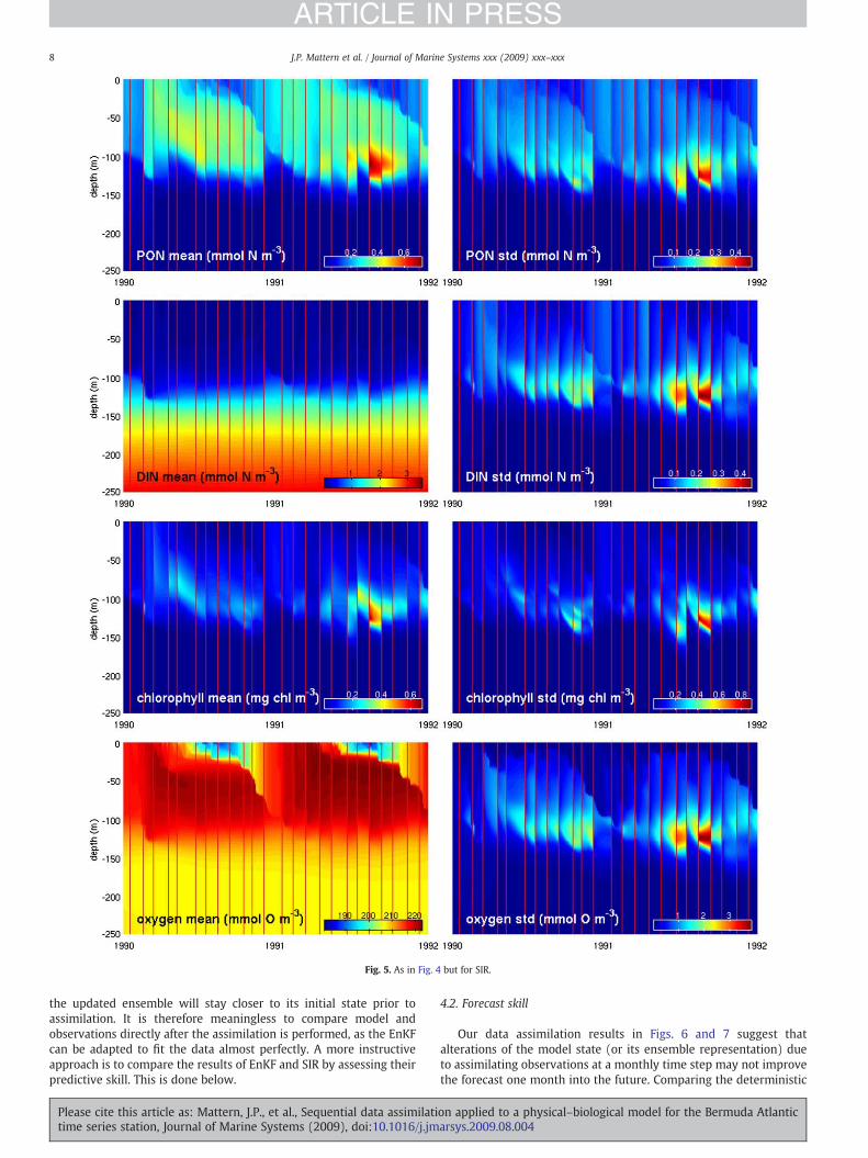
Fig. 5. As in Fig. 4 but for SIR.


ARTICLE IN PRESS

the updated ensemble will stay closer to its initial state prior toassimilation. It is therefore meaningless to compare model andobservations directly after the assimilation is performed, as the EnKFcan be adapted to fit the data almost perfectly. A more instructiveapproach is to compare the results of EnKF and SIR by assessing theirpredictive skill. This is done below.


4.2. Forecast skill

Our data assimilation results in Figs. 6 and 7 suggest thatalterations of the model state (or its ensemble representation) dueto assimilating observations at a monthly time step may not improvethe forecast one month into the future. Comparing the deterministic



Fig. 6. Ensemble distribution of the mean concentration of PON, DIN, chlorophyll and oxygen in the top 80 mwith EnKF data assimilation. The solid red line is the ensemble median,the dark gray area shows the regions between 0.25 and 0.75 quantile, and the light gray area marks the region between the ensemble minimum and maximum. EnKF assimilationsteps are marked by black vertical lines. Blue dots and error bars show the mean observations and their standard deviation in the top 80 m. Deterministic model run is shown as agreen dotted line. (For interpretation of the references to color in this figure legend, the reader is referred to the web version of this article.)


ARTICLE IN PRESS

simulation (green dashed line) and the ensemble median (red solidline), it appears that between the monthly BATS sampling dates themodel reverts back to a state close to that achieved without dataassimilation. This was also demonstrated with cross-validationexperiments (Mattern, 2008, results not shown). In order to assessthe predictive skill of our assimilation schemes at a shorter time scale,we make use of the BATS bloom cruise data. The bloom cruises were


intensive sampling periods in which observations were collectedbetween the dates of the monthly regular core cruises. For thepurposes of assessing forecast skill, we use the bloom cruise datapurely as validation data and not as part of the data assimilationprocedure. Specifically, we compute the root mean square error(RMSE) between the validation data and the predicted model outputfor those times (corresponding to a roughly 2 week forecast). These



Fig. 7. As in Fig. 6 but for SIR. (For interpretation of the references to color in this figure legend, the reader is referred to the web version of this article.)


ARTICLE IN PRESS

RMSEs are computed for the deterministic model run, as well as forour EnKF implementation and the 2 SIR implementations introducedin Section 3.2. This is done for each data assimilation technique and fordifferent ensemble sizes, namely nens=5, 10, 20, 40, 80, and for eachof the prognostic variables. The results are shown in Table 4. In eachcase, 20 replicate runs were carried out so that the standard deviationof the RMSE results could be computed and the Monte Carlo variationassessed.

The results in Table 4 demonstrate that a significant improvementin the predictive ability of the biological model can be achieved with


both the EnKF and SIR procedures. The improvement is most evidentfor Chl (using the EnKF and the Separate Variables SIR implementa-tion), as well as for PON (using the EnKF). The stronger updating ofthe ensemble mean towards the observations by the EnKF dataassimilation appears to lead to a more positive impact on thepredictive skill; the EnKF results for ensemble sizes greater than 10are better than the equivalent SIR results, especially for PON. It isnotable that the model results for oxygen cannot be significantlyimproved by any of the data assimilation techniques. This is consistentwith the result of our stochastic simulations, where the variation of



Table 4Root mean square error (RMSE) between BATS bloom observations and correspondingmodel output for the deterministic model with the optimized parameter set and for 3assimilation implementations and different ensemble sizes.

nens EnKF SIR SIR (separate) Deterministic

PON (mmol Nm−3)5 0.187±0.019 0.200±0.012 0.210±0.017 0.19810 0.176±0.008 0.197±0.012 0.200±0.01120 0.173±0.006 0.191±0.006 0.190±0.01040 0.172±0.005 0.190±0.007 0.190±0.00880 0.172±0.003 0.192±0.008 0.184±0.008

DIN (mmol Nm−3)5 0.735±0.024 0.761±0.014 0.752±0.021 0.75710 0.732±0.023 0.754±0.011 0.748±0.01620 0.730±0.019 0.756±0.006 0.752±0.01540 0.740±0.018 0.752±0.006 0.754±0.01580 0.742±0.012 0.753±0.005 0.751±0.012

Chlorophyll (mg chlorophyll a m−3)5 0.092±0.007 0.113±0.011 0.110±0.011 0.10410 0.096±0.007 0.112±0.009 0.103±0.01020 0.094±0.005 0.110±0.007 0.096±0.00640 0.093±0.003 0.110±0.006 0.096±0.00480 0.093±0.002 0.111±0.004 0.094±0.004

Oxygen (mmol O m−3)5 9.343±0.261 9.359±0.098 9.493±0.244 9.35010 9.294±0.229 9.328±0.103 9.451±0.12920 9.277±0.165 9.296±0.078 9.516±0.15040 9.342±0.135 9.255±0.075 9.561±0.15780 9.339±0.105 9.254±0.081 9.549±0.168

Each cell contains the mean and standard deviation of 20 ensemble runs. nens is theensemble size.


ARTICLE IN PRESS

the chosen biological parameters did not create a large ensemblespread for oxygen (see Supplementary Online Material). Thecomparison between the 2 different SIR implementations revealsthat the standard All Variables SIR implementation produces results asgood as those produced by the Separate Variables SIR, except for Chlwhere the latter technique performs better.

Ensemble size is a key practical consideration in sequential dataassimilation, trading off accuracy against computational cost. Table 4also considers the predictive skill using various ensemble sizes,including an assessment of the Monte Carlo variability of the resultsthrough replicate runs. For very small ensembles, with 5 or 10ensemble members, the predictive skill is poorer and the replicationerror (standard deviation) larger, especially for the EnKF. Increasingthe ensemble size decreases the prediction error and its standarddeviation. However, it is seen that for ensemble sizes of 20 andgreater, a doubling of the ensemble size does not change thepredictive skill significantly but doubles the computational cost(which scales linearly with ensemble size). However, the increase inensemble size shows a positive effect on the standard deviation; formost variables it decreases at a rate roughly equal to the inversesquare root of the ensemble size.

Another important feature in the assimilation of multivariate time-series data is illustrated in our application. Consider that theperformance of our standard (All Variables) SIR implementation forChl in Table 4 is poor compared to the other 2 implementations.This indicates that the chlorophyll profiles are resampled disadvan-tageously during the SIR's update step. In the SIR update procedure,ensemblemembers can have a high probability of being resampled if apoor fit for certain variables is compensated by a good fit for othervariables. In our case, poor chlorophyll profiles are resampled incombination with good PON profiles. This is likely indicative ofdynamical inconsistencies in the biological model formulation. In theapplication of the EnKF for multivariate data assimilation thegeneration of new ensembles allows the fit to improve for allvariables.


Finally, note that the results presented here are based onparameter variation following a specific log-normal distribution(Table 2). Experiments with other probability distributions, e.g. atruncated Gaussian, showed that the results are quite sensitive to thedistribution chosen (Mattern, 2008). Since it is often difficult to assignthese distributions accurately, we remark briefly on the consequencesof their mis-specification. At a basic level, the SIR procedure needs asufficient forecast ensemble spread, and thus requires an appropriateparameter distribution, to support this feature. This idea is illustratedin Figs. 6 and 7, where at the observation (or assimilation) times theforecast spread generally brackets the observation (or, in the case ofoxygen, the forecast ensemble spread and the observation error barsoverlap). If the ensemble spread is too small, the resampling step inthe SIR leads only to limited improvement and the result suffers. Thisimplies, however, that the model errors have been underestimated.The EnKF, on the other hand, can transform the ensemble out of itsprevious range upon update, even if model errors have beenunderestimated. The EnKF, however, is more sensitive to bothobservational data outliers and ensemble outliers. For the former,the EnKF will force the ensemble to trend towards extremeobservations. In the latter case, where an improbable combinationof extreme parameters produces an ensemble outlier, e.g. unrealisticprofiles, the outcome of the EnKF update can be affected detrimen-tally, especially for small ensemble sizes. (We encountered this duringone EnKF ensemble run where we had to remove an extremely highchlorophyll profile from the analysis.) The SIR is a more robustprocedure in this respect, as ensemble outliers that are far from thedata are assigned a low weight during the resampling step, and henceare unlikely to be propagated forward.

5. Discussion and conclusions

In this study we examined the application of 2 major sequentialdata assimilation techniques, the EnKF and SIR to a 1D coupledphysical–biological ocean model for the long-term ocean monitoringsite off Bermuda (BATS, Steinberg et al., 2001). We choose the 1Dmodel as a compromise between realism in describing the biology andphysics of our test site versus the computational considerationsinherent in these ensemble-based Monte Carlo methods. To date, theEnKF has found a wider range of applications in the context ofbiological models (e.g. Allen et al., 2003; Natvik and Evensen, 2003;Lenartz et al., 2007), whereas the SIR has been used less frequentlyand in the context of simpler 0D models (Losa et al., 2003; Dowd,2007). The novelty of this study hence lies in its use of SIR for dataassimilation in a partial differential equation based physical–biolog-ical model, and its comparison and contrast with the EnKF, in thecontext of estimation and prediction. However, the approachesconsidered here should be scaleable to higher dimensional problems,e.g. the ocean general circulationmodel used for ensemble-based dataassimilation by Brusdal et al. (2003).

In our implementation of sequential data assimilation, we havefocused on the biological components only. The physical–biologicalcoupling in our model is one-way: the physical model affectsbiological distributions through turbulent mixing, but the biologicalvariables do not feed back to the model physics. With nudging ofmodel temperature and salinity to the time-series observations fromthe BATS site, the physical model is able to adequately recreate keyphysical features such as the mixed layer depth; this suggests that themodel can be useful for short-term predictions of biological propertiesat the BATS site. As an extension, the distribution and time evolutionof the biological variables also contain information that could refinethe physical state, say by appending the state to include physicalvariables as well as biological ones.

We proceeded with ensemble generation by considering varia-tions in a subset of the biological parameters (chosen based on asensitivity analysis) as a dominant source of uncertainty or error (Lek,




ARTICLE IN PRESS

2007). After assigning probability distributions (log-normals) to theseparameters, we sampled randomly from these in order to generateensemble members. See Turner et al. (2008) for a general discussionon ensemble generation and error incorporation. Joint state andparameter estimation is also possible for stochastic dynamics. For SIR,state augmentation approaches for this have been developed(Kitagawa, 1998; Ionides et al., 2006); for the EnKF, similar methodsare also possible (Annan et al., 2005; Moradkhani et al., 2005).

After ensemble generation, the EnKF and SIR provide an updatestep to assimilate available observations. While both procedures canbe readily applied to a biological model, they operate quite differently.The EnKF incrementally updates the model state through the matrix-based Kalman filter updating equations (Evensen, 2006), while SIR is aweighted bootstrap procedure based on a likelihood function (Risticet al., 2004). Note that these nonlinear filtering problems are distinctfrom fully Bayesian approaches which assign priors to parameters andrely on computationally intensiveMarkov ChainMonte Carlo (MCMC)algorithms (e.g. Dowd and Meyer, 2003).

In both techniques, one must carefully consider implementationdetails, such as the scaling (or sample variances) assigned to theobservations and model outputs, otherwise a single variable type orobservation can dominate the analysis. For the EnKF, the errorcovariance matrix of the forecast ensemble was formed and thematrix-based updating equation applied. For SIR, the likelihoodfunction was defined on the basis of a multivariate normaldistribution and resampling was done on the ensemble of profiles;it is possible that more suitable distributions could be identified thattake better account of the discrepancy between observed andmodelled profiles. In fact, a key feature of a successful SIR withsmall ensemble sizes is that the forecast distribution must overlapwith the likelihood; this depends on both the parameter variation inthe stochastic simulation, as well as the assigned observation errorvariance.

Our experiments used real time-series data from BATS. This ischallenging since outliers are inevitably present, as are biases due tothe model's inability to explain all features present in the observa-tions. Both procedures appear robust. We also considered differentimplementations of SIR. In our All Variables SIR implementation,ensemble members are resampled to preserve the relations betweenthe biological variables. In our Separate Variables SIR, we resampledeach of the biological variables individually and independently at thecost of losing the dependencies between the variables during theupdate, in order to investigate a possible improvement in fit.

Our data assimilation experiments showed differences in perfor-mance between our implementations of the EnKF and the SIR. Whencompared to SIR, the EnKF update had a more pronounced effect inchanging the ensemble from forecast to update; the mean was shiftedmore and the standard deviation was greatly reduced after theupdate. One reason for this is that the SIR update does not generatenew ensembles (it simply resamples with replacement from the set ofcandidates provided by the forecast), whereas the EnKF generates anew set of ensemble members.

We investigated the effect of ensemble size, as it is a keydeterminant for performance. Generally we anticipate that largerensembles give better answers (i.e. more samples better characterizethe target distributions, or its moments), but they come at a highercomputational cost. Our ensemble sizes ranged from 5 to 80. As alower bound, we found that ensembles of 10 or fewer members aretoo small for reliable results. On the other hand, increasing theensemble size above 20 resulted in only a slight decrease in errorbetween the model output and the observations, suggesting that 20 isthe optimal ensemble size for our application. We anticipate that theoptimal ensemble size is specific to each application and may behigher for 3-dimensional models. Previously published studies thathave applied the EnKF to coupled physical–biological models haveused ensemble sizes of 100 to 200 (Allen et al., 2003; Evensen, 2003);


ensemble forecasts in numerical weather prediction typically usefewer than 100 ensemble members (Gneiting and Raftery, 2005).

Our experiments indicate that the predictive skill improved for a2-week forecast for both the EnKF and SIR in comparison to thedeterministic model run. We assessed the forecast ability bycomparing model output to observations obtained during intensivesampling periods when approximately bi-weekly data was available.The results suggest that the strong update of the model state closertowards observations in our EnKF implementation has a positiveeffect on the predictive skill. We also found that the forecast skill ofour standard SIR procedure can be improved by resampling eachvariable separately. The improvement in forecast skill is variable-dependent. Forecasts of PON and chlorophyll profit most from thedata assimilation, while no measurable improvement for oxygen wasfound.

The forecast skill of our application could likely be improved byreducing dynamical inconsistencies between our model and the BATSsystem. The 1D model is not able to capture some of the complexphysical dynamics present at the BATS site, such as the influence ofmesoscale eddies (McGillicuddy et al., 1998), and the biologicaldynamics have been highly simplified. Another important factor is theuncertainty assigned to the BATS observations, which is not accuratelyknown. We approximated this uncertainty based on the variability inthe observations. Both procedures are affected by this observationuncertainty — the EnKF through the observation error covariancematrix and the SIR through the likelihood specification. These controlhow closely the ensemble can move toward the observations at theupdate step.

In summary, the SIR and the EnKF improved model results andforecast abilities for the coupled physical–biological system weexamined. Several choices had to be made during the application ofboth assimilation techniques to a specific system, e.g. the observationerror covariance matrix and the likelihood function, which affectassimilation performance. In order to utilize the full improvement inthe predictive skill that sequential data assimilation can offer, themodel under consideration should be both well-calibrated (e.g.through parameter optimization) and also consistent with the systemof interest. For the BATS site, future work would therefore begin byrefining the physical and biological structure of the model. Our resultshowever demonstrate that ensemble-based data assimilation is apromising direction for improving prediction in coupled physical–biological systems.

Acknowledgments

Katja Fennel and Paul Mattern were supported by ONRMURI grantN00014-06-1-0739. Paul Mattern was also supported by NationalProgram for Complex Data Structures (NPCDS). Mike Dowd wassupported by both NSERC and NPCDS.We thank Jill Falkenberg for herassistance in preparing BATS data for assimilation. We also thank twoanonymous reviewers for constructive comments.

Appendix A. Supplementary data

Supplementary data associated with this article can be found, inthe online version, at doi:10.1016/j.jmarsys.2009.08.004.

References

Allen, J., Eknes, M., Evensen, G., 2003. An Ensemble Kalman Filter with a complexmarine ecosystem model: hindcasting phytoplankton in the Cretan Sea. AnnalesGeophysicae 21 (1), 399–411.

Annan, J., Hargreaves, J., Edwards, N., Marsh, R., 2005. Parameter estimation in anintermediate complexity earth system model using an ensemble Kalman filter.Ocean Modelling 8 (1–2), 135–154.

Arhonditsis, G., Brett, M., 2004. Evaluation of the current state of mechanistic aquaticbiogeochemical modeling. Marine Ecology Progress Series 271, 13–26.




ARTICLE IN PRESS

Arulampalam, M., Maskell, S., Gordon, N., Clapp, T., Sci, D., Organ, T., Adelaide, S., 2002. Atutorial on particle filters for online nonlinear/non-GaussianBayesian tracking. IEEETransactions on Signal Processing 50 (2), 174–188.

Bertino, L., Evensen, G., Wackernagel, H., 2003. Sequential data assimilation techniquesin oceanography. International Statistical Review 71 (2), 223–241.

Brusdal, K., Brankart, J., Halberstadt, G., Evensen, G., Brasseur, P., van Leeuwen, P.,Dombrowsky, E., Verron, J., 2003. A demonstration of ensemble-based assimilationmethods with a layered OGCM from the perspective of operational oceanforecasting systems. Journal of Marine Systems 40, 253–289.

Burchard, H., Bolding, K., Villarreal, M., 1999. GOTM — a general ocean turbulencemodel. Theory, applications and test cases. European Commission report EUR18745.

Doney, S., Lima, I., Lindsay, K., Moore, J., Dutkiewicz, S., Friedrichs, M., Matear, R., 2001.Marine biogeochemical modeling: recent advances and future challenges.Oceanography 14 (4), 93–107.

Dowd, M., 2007. Bayesian statistical data assimilation for ecosystem models usingMarkov Chain Monte Carlo. Journal of Marine Systems 68 (3–4), 439–456.

Dowd, M., Meyer, R., 2003. A Bayesian approach to the ecosystem inverse problem.Ecological Modelling 168 (1–2), 39–55.

Evensen, G., 2003. The Ensemble Kalman Filter: theoretical formulation and practicalimplementation. Ocean Dynamics 53 (4), 343–367.

Evensen, G., 2006. Data Assimilation: The Ensemble Kalman Filter. Springer Verlag NewYork, Inc., Secaucus, NJ, USA.

Fennel, K., Boss, E., 2003. Subsurface maxima of phytoplankton and chlorophyll: steady-state solutions from a simple model. Limnology and Oceanography 48 (4),1521–1534.

Fennel, K., Losch, M., Schröter, J., Wenzel, M., 2001. Testing a marine ecosystem model:sensitivity analysis and parameter optimization. Journal of Marine Systems 28 (1–2),45–63.

Fennel, K., Wilkin, J., Levin, J., Moisan, J., O'Reilly, J., Haidvogel, D., 2006. Nitrogen cyclingin the Middle Atlantic Bight: results from a three-dimensional model andimplications for the North Atlantic nitrogen budget. Global Biogeochemical Cycles20 (3). doi:10.1029/2005GB002456.

Fennel, K., Wilkin, J., Previdi, M., Najjar, R., 2008. Denitrification effects on air–sea CO2

flux in the coastal ocean: simulations for the Northwest North Atlantic. GeophysicalResearch Letters 35, L24608. doi:10.1029/2008GL036147.

Friedrichs, M., 2001. A data assimilative marine ecosystem model of the centralequatorial Pacific: numerical twin experiments. Journal of Marine Research 59,859–894.

Friedrichs, M., Dusenberry, J., Anderson, L., Armstrong, R., Chai, F., Christian, J., Doney, S.,Dunne, J., Fujii, A., Hood, R., et al., 2007. Assessment of skill and portability inregional marine biogeochemical models: role of multiple planktonic groups.Journal of Geophysical Research 112 (8). doi:10.1029/2006JC003852.

Garcia, H., Gordon, L., 1992. Oxygen solubility in seawater: better fitting equations.Limnology and Oceanography 37 (6), 1307–1312.

Geider, R., MacIntyre, H., Kana, T., 1996. A dynamic model of photoadaptation inphytoplankton. Limnology and Oceanography 41 (1), 1–15.

Geider, R., MacIntyre, H., Kana, T., 1997. Dynamic model of phytoplankton growth andacclimation: responses of the balanced growth rate and the chlorophyll a: carbonratio to light, nutrient-limitation and temperature. Marine Ecology Progress Series148 (1), 187–200.

Gneiting, T., Raftery, A., 2005.Weather forecasting with ensemblemethods. Science 310(5746), 248–249.

Gordon, N., Salmond, D., Smith, A., 1993. Novel approach to nonlinear/non-GaussianBayesian state estimation. Radar and Signal Processing, IEE Proceedings F 140 (2),107–113.

Hofmann, E., Friedrichs, M., 2001. Biogeochemical data assimilation. Encyclopedia ofOcean Sciences 1, 302–308.

Ionides, E., Breto, C., King, A., 2006. Inference for nonlinear dynamical systems.Proceedings of the National Academy of Sciences 103 (49), 18438.


Kalnay, E., Kanamitsu, M., Kistler, R., Collins, W., Deaven, D., Gandin, L., Iredell, M., Saha,S., White, G., Woollen, J., et al., 1996. The NCEP/NCAR 40-Year Reanalysis Project.Bulletin of the American Meteorological Society 77 (3), 437–471.

Kantha, L., 2004. A general ecosystem model for applications to primary productivityand carbon cycle studies in the global oceans. Ocean Modelling 6 (3–4), 285–334.

Kishi, M., Kashiwai, M., Ware, D., Megrey, B., Eslinger, D., Werner, F., Noguchi-Aita, M.,Azumaya, T., Fujii, M., Hashimoto, S., et al., 2007. NEMURO — a lower trophic levelmodel for theNorth Pacificmarine ecosystem. EcologicalModelling 202 (1–2), 12–25.

Kitagawa, G., 1996. Monte Carlo filter and smoother for non-Gaussian nonlinear statespace models. Journal of Computational and Graphical Statistics 5 (1), 1–25.

Kitagawa, G., 1998. A self-organizing state-space model. Journal of the AmericanStatistical Association 93 (443), 1203–1215.

Lawson, L., Hofmann, E., Spitz, Y., 1996. Time series sampling and data assimilation in asimple marine ecosystem model. Deep Sea Research Part II: Topical Studies inOceanography 43 (2), 625–651.

Lek, S., 2007. Uncertainty in ecological models. Ecological Modelling 207 (1), 1–2.Lenartz, F., Raick, C., Soetaert, K., Grégoire, M., 2007. Application of an Ensemble Kalman

filter to a 1-D coupled hydrodynamic-ecosystem model of the Ligurian Sea. Journalof Marine Systems 68 (3–4), 327–348.

Losa, S., Kivman, G., Schröter, J., Wenzel, M., 2003. Sequential weak constraintparameter estimation in an ecosystem model. Journal of Marine Systems 43 (1–2),31–49.

Mattern, J.P., 2008. Ensemble-based data assimilation for a physical–biological oceanmodel near Bermuda. Master's thesis, Universität zu Lübeck.

McGillicuddy, D., Robinson, A., Siegel, D., Jannasch, H., Johnson, R., Dickey, T., McNeil, J.,Michaels, A., Knap, A., 1998. Influence of mesoscale eddies on new production inthe Sargasso Sea. Nature 394, 263.

McGillicuddy Jr., D., Anderson, L., Doney, S., Maltrud, M., 2003. Eddy-driven sources andsinks of nutrients in the upper ocean: results from a 0.1 resolution model of theNorth Atlantic. Global Biogeochemical Cycles 17 (2). doi:10.1029/2002GB001987.

Moradkhani, H., Sorooshian, S., Gupta, H., Houser, P., 2005. Dual state–parameterestimation of hydrological models using ensemble Kalman filter. Advances inWater Resources 28 (2), 135–147.

Natvik, L., Evensen, G., 2003. Assimilation of ocean colour data into a biochemical modelof the North Atlantic Part 1. Data assimilation experiments. Journal of MarineSystems 40, 127–153.

Ristic, B., Arulampalam, S., Gordon, N., 2004. Beyond the Kalman filter: particle filtersfor tracking applications. Artech House.

Rodi, W., 1987. Examples of calculation methods for flow andmixing in stratified fluids.Journal of Geophysical Research 92 (C5), 5305–5328.

Rothstein, L., Cullen, J., Abbott, M., Chassignet, E., Denman, K., Doney, S., Ducklow, H.,Fennel, K., Follows, M., Haidvogel, D., Hoffman, E., Karl, D., Kindle, J., Lima, I., Maltrud,M., McClain, C., McGillicuddy, D., Olascoaga, J., Spitz, Y., Wiggert, J., Yoder, J., 2006.Modeling ocean ecosystems: the PARADIGM program. Oceanography 19 (1), 16–45.

Schartau, M., Oschlies, A., Willebrand, J., 2001. Parameter estimates of a zero-dimensional ecosystem model applying the adjoint method. Deep-Sea ResearchPart II 48 (8–9), 1769–1800.

Spitz, Y., Moisan, J., Abbott, M., 2001. Configuring an ecosystem model using data fromthe Bermuda Atlantic Time Series (BATS). Deep-Sea Research Part II 48 (8–9),1733–1768.

Steinberg, D., Carlson, C., Bates, N., Johnson, R.,Michaels, A., Knap, A., 2001. Overviewof theUS JGOFS Bermuda Atlantic Time-series Study (BATS): a decade-scale look at oceanbiology and biogeochemistry. Deep-Sea Research Part II 48 (8–9), 1405–1447.

Turner, M., Walker, J., Oke, P., 2008. Ensemble member generation for sequential dataassimilation. Remote Sensing of Environment 112 (4), 1421–1433.

Wanninkhof, R., 1992. Relationship between wind speed and gas exchange over theocean. Journal of Geophysical Research 97 (C5), 7373–7382.

Wiggert, J., Murtugudde, R., Christian, J., 2006. Annual ecosystem variability in thetropical Indian Ocean: results of a coupled bio-physical ocean general circulationmodel. Deep-Sea Research Part II 53 (5–7), 644–676.


http://dx.doi.org/10.1029/2005GB002456

http://dx.doi.org/10.1029/2008GL036147

http://dx.doi.org/10.1029/2006JC003852

http://dx.doi.org/10.1029/2002GB001987


article in press - dalhousie's marine …memg.ocean.dal.ca/memg/pubs/mattern_et_al_2009.pdf ·...

Documents