article optimization strategy of electric vehicles

Article

Optimization Strategy of Electric Vehicles Charging

Path Based on " Traffic-Price-Distribution " Mode Wanhao Yang1, Hong Wang 2, Zhijie Wang 1,*, Xiaolin Fu 1, Pengchi Ma1, Zhengchen Deng3, Zihao Yang 4 1.College of Electrical Engineering, Shanghai Dianji University, Shanghai 201306,China;

[email protected] (W.Y.); [email protected](X.F.); [email protected] (P.M.)

2. School of Economics & Management, Tongji University, Shanghai 200092, China; [email protected]

3. College of Electrical Engineering, Shanghai University of Electric Power, Shanghai 200090,China;

[email protected]

4. College of Electrical and Electronic Engineering, North China Electric Power University, Beijing

102206,China; [email protected]

* Correspondence: [email protected]; Tel.: +86-189-6458-6826

Abstract: Aiming at the current optimization problem of electric vehicle charging path planning, a charging path optimization strategy for electric vehicles under the "Traffic-Price-Distribution" mode is proposed. This strategy builds an electric vehicle charging and navigation system based on road traffic network model, real-time electricity price model and distribution network model. Based on Dijkstra shortest path algorithm and Monte Carlo time-space prediction method, the goal is to minimize the charging cost of electric vehicles. Optimal charging path. The simulation results of MATLAB and MATPOWER show that the electric vehicle charging path optimization strategy can better solve the local traffic congestion problem and improve the safety and stability of the distribution network on the basic of fully considering the convenience of electric vehicle charging.

Keywords: electric vehicles charging navigation system; charging path; road transportation network; distribution network; real-time electricity price

1. Introduction

With the development of industrialization, the global awareness of the energy crisis is increasing. Compared with the current depletion of traditional petroleum resources, electric vehicles, as a low-carbon green vehicle driven by electricity, will undoubtedly save energy Ranking research trends [1]. Due to the unique charging characteristics of electric vehicles, the charging behavior of large-scale electric vehicles not only puts pressure on the transportation system, but also affects the safe and stable operation of the distribution network [2]. This paper focuses on the comprehensive impact of real-time electricity price mechanism, transportation network and distribution network on the charging behavior of electric vehicle users. At present, by referring to existing literature, I found that research on electric vehicles is mainly divided into the following two aspects:

The current research focuses on the impact of electric vehicles on the grid [3-9]. (a) Analyze the influence of electric vehicle charging stations on grid harmonics [3,4]. Gao, C.W. analyzed the changes of the electric grid under the charging behavior of electric vehicles [5]. (b) Make in-depth research on the impact of electric vehicles on the grid load [6,7]. Shao, Y.C. further analyzed the spatio-temporal prediction of the charging load of large-scale electric vehicles under the "vehicle-network-road" model and its impact on the power distribution flow [8]. (c) Propose a new mode of power system operation in response to the changing operation requirements of the current distribution network [9]. On the other hand, the impact of electric vehicle charging behavior on the

Preprints (www.preprints.org) | NOT PEER-REVIEWED | Posted: 30 November 2019

© 2019 by the author(s). Distributed under a Creative Commons CC BY license.

Peer-reviewed version available at Energies 2020, 13, 3208; doi:10.3390/en13123208

mailto:[email protected](X.F.)

http://creativecommons.org/licenses/by/4.0/

https://doi.org/10.3390/en13123208

transportation network is addressed. (d) Establish the comprehensive urban road congestion evaluation system for the first time [10]. Kobayashi Yuichi identified an electric vehicle charging path planning method based on the starting and ending traffic locations of an electric vehicle and actual traffic congestion [11]. (e) Consider the electric vehicle charging path planning under the real-time dynamic energy consumption of electric vehicles [12].

At present, research on the charging path planning of large-scale electric vehicles based on traffic conditions and distribution network conditions is still very rare. Luo, Y.G. proposed a charging path planning strategy combining transportation network and distribution network [13]. Yan, Y.Y. and others further put forward the idea of combining electric vehicles, distribution networks, and transportation networks into a "vehicle-network-road" system, and initially discussed the optimal charging path planning technology for electric vehicles [14]. (f) Formulate an orderly charging scheduling strategy for electric vehicles that simultaneously improves transportation and grid operation performance [15]. (g) Propose a charging navigation idea that introduced real-time electricity prices [16]. However, the comprehensive impact of real-time electricity price mechanism on transportation network, distribution network and user charging behavior has not been further studied.The main innovations of this paper can be summarized as follows:

1. Based on previous research, this paper develops a more comprehensive real-time electricity price mechanism, and builds a "road-price-network" model through MATLAB simulation technology. This paper proposes a method that not only fully considers the information interaction between the transportation network and the distribution network, but optimize the path optimization strategy for electric vehicle charging.

2. The optimal charging path recommended by the optimization strategy can better solve the problems of traffic congestion, uneven load distribution of charging stations, and safety of distribution network operation while reducing the charging cost of large-scale electric vehicle groups.

3. The above model is used to optimize the intelligent charging planning of the "Internet of Vehicles" platform in Taizhou, Jiangsu Province, China.

2. "Road traffic network-real-time electricity price-distribution network" system model

2.1 Road traffic network model

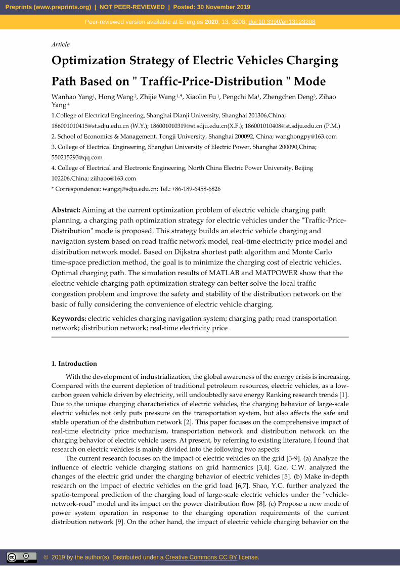
Based on the previous research, this paper builds a "road transportation network-real-time electricity price-distribution network" system model and conducts research on the optimal path navigation of electric vehicles. It is assumed that all electric vehicles adopt the form of fast charging, and its unique charging characteristics and space characteristics have a certain impact on the road transportation network and distribution network. The relationship between each other is shown in Figure 1.

Road traffic network Real-time electricity prices

Distribution network

Spatio-temporal prediction model of electric vehicle

charging load

Charging characteristics

Spatial characteristics

Electric vehicle charging navigation system

Figure 1. Relationship between subsystems



https://doi.org/10.3390/en13123208

2.1.1 Road topology

Let Rn=(Nd,S,L,V,Q,K) represent the road network. Nd is the set of road crossing nodes in the road network system, and the topological structure of

the traffic network is shown by taking Figure 2 as an example.

Figure 2. Traffic network topology diagram

S is the adjacency matrix set of road weights, which is used to describe the length of each road segment and the connection relationship between nodes:

, 0, ,( , ) 0 =y

inf, ,

xy xyl l x yS x y x

x y

≠

=

路段( )的长度

，

路段( )不连通

(1)

Where lxy is the length of the link between adjacent nodes x and y; inf represents infinity, that is, the two nodes are not adjacent. When the road network model is assumed to be a two-lane channel,

( , ) ( , ) , , ,xyS x y S y x l x y N x y= = ∀ ∈ ≠ (2)

According to the matrix S generated in Figure 2, under the Dijkstra shortest path algorithm, the shortest path between nodes is obtained.

12 13

21 24 25

31 34 36

42 43 47

0 inf inf inf inf inf inf 0 inf inf inf inf inf inf 0 inf inf inf inf

inf 0 inf inf inf infS i

l ll l ll l l

l l l= 52 57

63 67 68

74 75 76 79

86 89

nf inf inf 0 inf inf inf inf inf inf inf 0 inf inf inf inf 0 inf inf inf inf inf inf inf 0 inf inf inf

l ll l l

l l l ll l

97 98inf inf inf 0 l l

(3)

2.1.2 Speed-Density Model

L is the road grade of the road section. Divided into 5 road levels. The traffic density is K=N/L, and the traffic flow is Q=N/T. Road speed is determined by both road grade and traffic flow.

Table 1. Road grade Road grade Vm/(km/h) Q /( Traffic /h)

1 80 1200 2 60 900 3 50 660 4 40 660 5 30 540

Literature [17] From the urban road traffic speed-density model [18], we can get:



https://doi.org/10.3390/en13123208

( / )

ln( / )(Blocking flow)

(Free flow)m

m j

K Kf

V K KV

V e−

=

(4)

Greenberg's logarithmic model and Underwood's exponential model are applicable to blocking flow and own flow, respectively. The curves of the two models intersect in the middle and the traffic density at the intersection is K0. A logarithmic model is used for the obstructed flow (left of the intersection); an exponential model is used for the free flow (right of the intersection). Among them, Vm is the zero-flow speed, Km is the optimal density at the maximum traffic volume, Vf is the ideal smooth speed, and Kj is the maximum traffic density.

Available traffic flow formula:

( / )

ln( / ), (Blocking flow)

, (Free flow)j m

m j

K Kf

KV K KQ KV

KV e−

= =

(5)

Define the road congestion rate ρ=1/V, which means road congestion.

2.1.3 OD analysis method

The vehicle OD matrix is an important data in the prediction and analysis of electric vehicle traffic distribution. This paper adopts the OD back-calculation matrix based on mathematical programming method [19], that is, to estimate the distribution of trips in the road network by the traffic flow of the road section. For a certain road network, two or two nodes are first matched as a start-end point pair. Assume that the traffic allocated on the road section at a time is Yi(i=1、2、…、

n)), Yi can be expressed as a linear combination of Xj: Yi=Pi1X1+Pi2X2…+PinXn (6)

Pin is expressed as the distribution ratio of the n-th starting and ending points to the travel distribution amount on the link i.

The traffic distribution of all road sections is as follows [20]:

11 1 2 2 1

21 1 2 2 2

1 1 2 2

1 1

2 2

n n

n n

mm m mn n

Y P X P X P XY P X P X P X

Y P X P X P X

= + …+= + …+

= + … +L

(7)

The OD probability matrix is: PX=Y (8)

By performing inverse calculation on formula (8), X=P-1Y is obtained, X is the inverse OD travel matrix obtained by the inverse OD mode, and Y is the road flow matrix distributed at the current time. Assume that the current number of road sections is m, and the number of pairs of start and end points is n.

Solve:

2 2

1 1 1m = ( ')in ( )

m m n

i i j jj ii i j

S P X Yf X= = =

= −∑ ∑ ∑

(9)

Among them:

' '

1( 1 2 )

n

i i i ij j ij

S Y Y P X Y j n=

= − = − =∑ L、、

(10)

Yi ’is the actual road flow. The system of equations consisting of m equations containing n travel distributions can be reduced to a system of n-order equations with only one unknown quantity. Through the above mathematical programming method, a unique OD travel matrix X is obtained. Electric vehicles can simulate their driving routes under the OD matrix.

2.2 Real-time electricity price model



https://doi.org/10.3390/en13123208

Electricity price fluctuations and demand interact with each other. Charging stations set prices in a short time interval (10min). Charging cars grasp the real-time changes in electricity prices by interacting with charging stations. The price elasticity coefficient e is a standardized quantity of the relationship between price and load change. Based on the Customer Satisfaction (ACSI) model [20], the expected satisfaction δ for electric vehicle charging is obtained, and the quantitative relationship [21] between the two is approximated by the revised price elasticity coefficient e’=e+δ.

2.2.1 Load elasticity coefficient

( / ) ( / ) / ( / )s s t te p m p p m m= ∂ ∂ = ∆ ∆ (11)

In the formula: Δm and Δp respectively represent the micro increment of the electric vehicle charging load and the fluctuation of the electricity price; s and t represent the charging station number, and s=t represents the elasticity of the electricity price of the electric vehicle charging load of the current charging station to the charging station (since Load elasticity), when s≠t, it means the current price of the charging station is elastic to the price of other charging stations (cross-load elasticity); s, t=0,1,2,…,n. The real-time electricity price elasticity matrix of the charging station is expressed as:

11 1

1

n

n nn

e eE

e e

=

LM O M

L

(12)

The dynamic demand response of the load and the real-time electricity price elasticity are less than approximately a first-order linear relationship, that is, the electricity price elasticity coefficient remains unchanged within each time period (10min).

2.2.2 Construction of Electric Vehicle Charging Satisfaction Model δ

Based on the ACSI model, δ takes into account the cost savings of electric vehicle charging, the three factors of arrival distance and charging queue time, which are defined as the weighting factor fcost of the electric vehicle charging, the distance factor farrival, and the queuing time factor fqueue. Value, the δ expression is as follows:

co2 2

s= arrival q e et u uaf bf cfδ + +

(13)

In the formula: a，b，c are weighting coefficients, a+b+c=1, fcost is the first-level indicator, farrival and fqueue are the second-level indicators.

The revised electricity price elasticity coefficient e’=e+δ, then the revised real-time electricity price price elasticity matrix of the charging station is expressed as:

' '11 1

' '1

'

n

n nn

e eE

e e

=

LM O M

L

(14)

Get the response formula of real-time electricity price of each charging station: '1 1 1 1 1'

2 2 2 22

'

/ /

' /n n n nn

p p m m pp m m pp

E

p m m pp

∆ ∆ = +

∆

O M MM

(15)

In the formula: p1,p2,…,pn are real-time prices immediately before the electricity price changes; p1’ ,p2’ ,…,pn’ are real-time electricity prices after changes.

2.2.3 Economic Benefits of Electric Vehicle Charging



https://doi.org/10.3390/en13123208

Electric vehicle electricity cost Q0 before real-time electricity price: Q0=p0M0 (16)

Among them, the fixed electricity price p0=0.65 yuan/kwh, M0represents the total load of electric vehicle charging.

Electricity charges Q1 for electric vehicles after real-time electricity prices:

11 1

=T n

ti tit i

Q p m= =∑∑

(17)

Among them, pti and mti represent the real-time electricity price and charging load of each charging station in each period, and T is the total number of periods.

Meet the inequality constraints of electric vehicle charging profit: Q1< Q0 (18)

2.3 Distribution Network Model

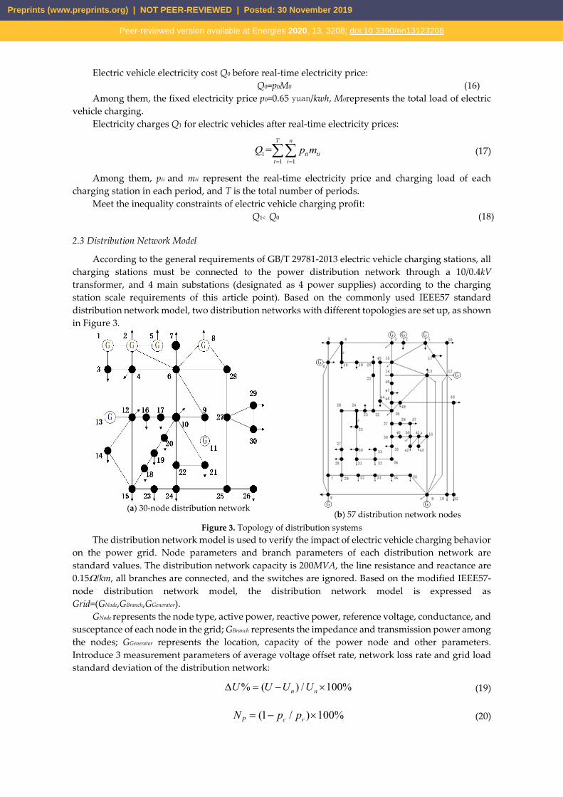
According to the general requirements of GB/T 29781-2013 electric vehicle charging stations, all charging stations must be connected to the power distribution network through a 10/0.4kV transformer, and 4 main substations (designated as 4 power supplies) according to the charging station scale requirements of this article point). Based on the commonly used IEEE57 standard distribution network model, two distribution networks with different topologies are set up, as shown in Figure 3.

(a) 30-node distribution network (b) 57 distribution network nodes

Figure 3. Topology of distribution systems The distribution network model is used to verify the impact of electric vehicle charging behavior

on the power grid. Node parameters and branch parameters of each distribution network are standard values. The distribution network capacity is 200MVA, the line resistance and reactance are 0.15Ω/km, all branches are connected, and the switches are ignored. Based on the modified IEEE57-node distribution network model, the distribution network model is expressed as Grid=(GNode,GBranch,GGenerator).

GNode represents the node type, active power, reactive power, reference voltage, conductance, and susceptance of each node in the grid; GBranch represents the impedance and transmission power among the nodes; GGenerator represents the location, capacity of the power node and other parameters. Introduce 3 measurement parameters of average voltage offset rate, network loss rate and grid load standard deviation of the distribution network:

% ( ) / 100%n nU U U U ×∆ = − (19)

(1 / ) 100%P c rN p p= − × (20)



https://doi.org/10.3390/en13123208

2

1

1 ( )n

i zi

m mn

σ=

= −∑

(21)

In the formula: rated voltage Un; actual voltage U; grid input power Pr; grid output power Pc; line average load mz; line load mi.

3.Spatio-temporal prediction model of electric vehicle charging load

3.1 Frame structure of spatio-temporal prediction of charging load

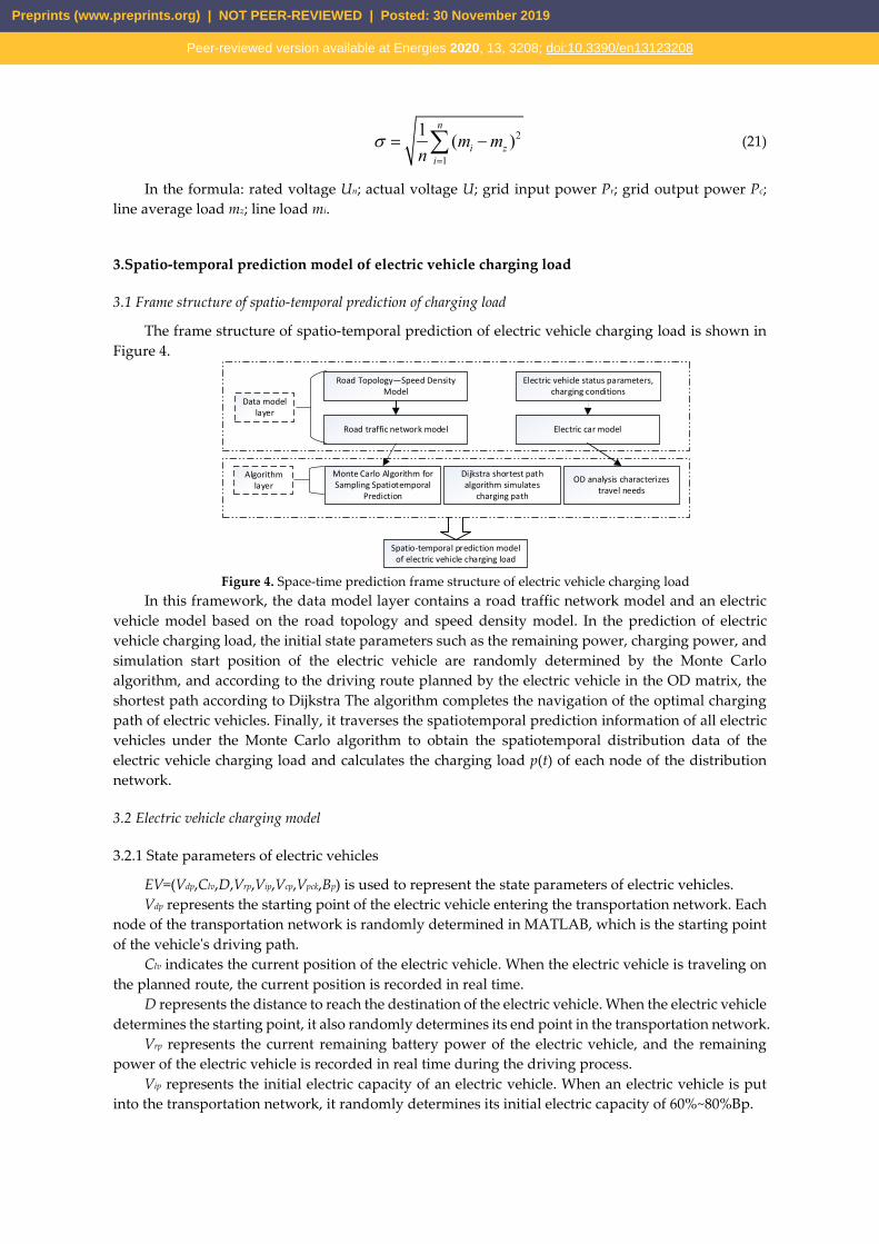
The frame structure of spatio-temporal prediction of electric vehicle charging load is shown in Figure 4.

Road Topology—Speed Density Model

Electric vehicle status parameters, charging conditions

Road traffic network model Electric car model

Monte Carlo Algorithm for Sampling Spatiotemporal

Prediction

Dijkstra shortest path algorithm simulates

charging path

Spatio-temporal prediction model of electric vehicle charging load

Data model layer

OD analysis characterizes travel needs

Algorithm layer

Figure 4. Space-time prediction frame structure of electric vehicle charging load

In this framework, the data model layer contains a road traffic network model and an electric vehicle model based on the road topology and speed density model. In the prediction of electric vehicle charging load, the initial state parameters such as the remaining power, charging power, and simulation start position of the electric vehicle are randomly determined by the Monte Carlo algorithm, and according to the driving route planned by the electric vehicle in the OD matrix, the shortest path according to Dijkstra The algorithm completes the navigation of the optimal charging path of electric vehicles. Finally, it traverses the spatiotemporal prediction information of all electric vehicles under the Monte Carlo algorithm to obtain the spatiotemporal distribution data of the electric vehicle charging load and calculates the charging load p(t) of each node of the distribution network.

3.2 Electric vehicle charging model

3.2.1 State parameters of electric vehicles

EV=(Vdp,Clv,D,Vrp,Vip,Vcp,Vpck,Bp) is used to represent the state parameters of electric vehicles. Vdp represents the starting point of the electric vehicle entering the transportation network. Each

node of the transportation network is randomly determined in MATLAB, which is the starting point of the vehicle's driving path.

Clv indicates the current position of the electric vehicle. When the electric vehicle is traveling on the planned route, the current position is recorded in real time.

D represents the distance to reach the destination of the electric vehicle. When the electric vehicle determines the starting point, it also randomly determines its end point in the transportation network.

Vrp represents the current remaining battery power of the electric vehicle, and the remaining power of the electric vehicle is recorded in real time during the driving process.

Vip represents the initial electric capacity of an electric vehicle. When an electric vehicle is put into the transportation network, it randomly determines its initial electric capacity of 60%~80%Bp.



https://doi.org/10.3390/en13123208

Vcpv is the charging power of electric vehicles. This article assumes that electric vehicles choose the fast charging method, and the charging can be completed within 0.5~1h, and the charging power is 45-60kW.

Vpck is the power consumption per kilometer of electric vehicles, and Vpck=0.2(kWh)/km. Bp is the battery power of the vehicle when fully charged, and the charging of the electric vehicle

battery is completed when it is fully charged. 3.2.2 Charging conditions Determine whether to charge based on the current electric vehicle status: 1) The electric vehicle residual power Vrp forces the electric vehicle to charge when it is below

30% of the battery power Bp [22]. 2) The remaining power of the electric vehicle cannot reach the designated destination. Time estimate. For an electric vehicle that needs to be charged, its complete power change

process:

1 1 1

2 2

3 1 2

4 3

= ( / ), 30%( / )i i pck p

i i

w

c

t l v D d V Bt l v

tt t t Tt t t

∑ − ≤

= ∑= = + +

= +

(22)

In the formula, t1 indicates the time that the electric vehicle has traveled from the departure to the current position; t2 indicates the time required to reach the charging station when the current position of the electric vehicle meets the charging conditions; Tw indicates the queue time of the electric vehicle at the charging station; tc=( Bp-Vrp) /Vcpv represents the time required for the electric vehicle battery to be fully charged.

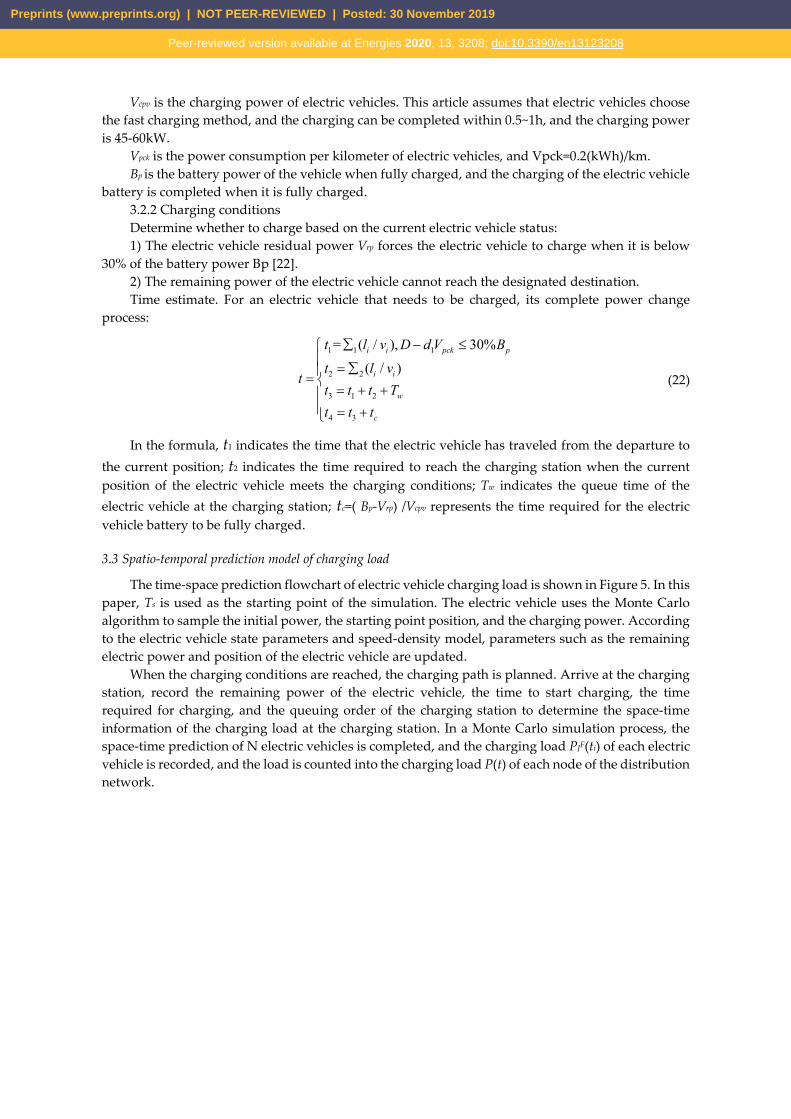
3.3 Spatio-temporal prediction model of charging load

The time-space prediction flowchart of electric vehicle charging load is shown in Figure 5. In this paper, Ts is used as the starting point of the simulation. The electric vehicle uses the Monte Carlo algorithm to sample the initial power, the starting point position, and the charging power. According to the electric vehicle state parameters and speed-density model, parameters such as the remaining electric power and position of the electric vehicle are updated.

When the charging conditions are reached, the charging path is planned. Arrive at the charging station, record the remaining power of the electric vehicle, the time to start charging, the time required for charging, and the queuing order of the charging station to determine the space-time information of the charging load at the charging station. In a Monte Carlo simulation process, the space-time prediction of N electric vehicles is completed, and the charging load PJF(ti) of each electric vehicle is recorded, and the load is counted into the charging load P(t) of each node of the distribution network.



https://doi.org/10.3390/en13123208

Get the number of EVs N

J =1

Start

Generate the electric vehicle charging power Vcpv, initial power Vip, simulation start time Ts, starting point position Vdp

Read the travel destination D generated by the corresponding OD probability matrix

Calculate the travel speed of each section according to the travel path and speed-density model

Electric vehicle charging path navigation

Update road flow, update remaining power Vrp, update simulation time T

J >N?

Recharged?

Calculate travel time t1

Reach the charging station to calculate the travel time t2, update the remaining power Vrp, and simulate the time T

Estimate the time required for fast charging tc

Determine the time and space information of fast charging at the charging station, and electric vehicles line up for charging in the order of arrival.Calculate the queue time Tw for electric vehicles

Update charging vehicle simulation time t4 after charging

J =J +1

Count the charging load of each node in the distribution networkP(t)

end

yesno

yes

no

Figure 5. Flow chart of electric vehicle charging load space-time prediction

The travel destination D generated by the electric vehicle corresponding to the OD matrix is read, and the travel speed of each road segment is calculated according to the travel path and the speed-density model. Calculate the travel time t1, update the road flow, the remaining power Vrp, and update the simulation time T. Determine whether the electric car has reached the charging conditions: the remaining electric power Vrp of the electric car is below 30% of the battery power Bp or the remaining electric power of the electric car cannot reach the designated destination. When the electric vehicle reaches the charging station, the travel time t2 is calculated, the remaining power Vrp is updated, and the simulation time T. You can estimate the time Tc required for fast charging. Determine the time and space information of the fast charging of the current charging station, and the electric vehicles are queued for charging in the order of arrival. The electric vehicle simulation time t4 is updated at the end of charging. In a Monte Carlo simulation process, the space-time prediction of N electric vehicles is completed, and the charging load PJF(ti) of each electric vehicle is recorded, and the load is counted into the charging load P(t)of each node of the distribution network.

3.4 Monte Carlo simulation convergence conditions

Based on the charging load spatio-temporal prediction model, with 10 minutes as a simulation interval, the Monte Carlo algorithm is used to obtain the simulation results of the spatiotemporal distribution of electric vehicles. The time tc, charging load ps, and charging start time Ts of each electric vehicle are recorded. According to the situation that each charging station is connected to the distribution network node, the charging load is calculated into the corresponding distribution



https://doi.org/10.3390/en13123208

network node. At time ti, the charging load PF(ti) of node F of the distribution network can be expressed as:

1( )= ( )

mF F

i n in

P t P t=∑

(23)

In the formula, m represents the number of electric vehicles connected to node F at time ti, and PJF(ti) represents the charging power of the J-th electric vehicle access node.

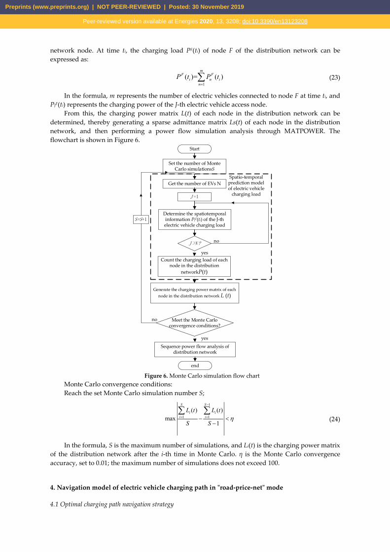
From this, the charging power matrix L(t) of each node in the distribution network can be determined, thereby generating a sparse admittance matrix Ls(t) of each node in the distribution network, and then performing a power flow simulation analysis through MATPOWER. The flowchart is shown in Figure 6.

Get the number of EVs N

J =1

Start

J >N ?

Count the charging load of each node in the distribution

networkP(t)

end

yes

no

Set the number of Monte Carlo simulationsS

Determine the spatiotemporal information PJF(ti) of the J-th electric vehicle charging load

Generate the charging power matrix of each node in the distribution network L (t)

Meet the Monte Carlo convergence conditions?

S=S+1

Sequence power flow analysis of distribution network

yes

no

Spatio-temporal prediction model of electric vehicle

charging load

Figure 6. Monte Carlo simulation flow chart

Monte Carlo convergence conditions: Reach the set Monte Carlo simulation number S;

1

1 1( ) ( )

max1

S S

i ii i

L t L t

S Sη

−

= = <−−

∑ ∑

(24)

In the formula, S is the maximum number of simulations, and Li(t) is the charging power matrix of the distribution network after the i-th time in Monte Carlo. η is the Monte Carlo convergence accuracy, set to 0.01; the maximum number of simulations does not exceed 100.

4. Navigation model of electric vehicle charging path in "road-price-net" mode

4.1 Optimal charging path navigation strategy



https://doi.org/10.3390/en13123208

To plan the optimal charging path for an electric vehicle under this electric vehicle charging path navigation model, you first need to determine traffic network parameters such as road length, road flow and driving speed, and EV parameters such as the starting point, initial power, and destination of the electric vehicle. For electric vehicles that require charging, plan their optimal charging path navigation; if there is no demand for electric vehicles, the electric vehicles will travel on the prescribed route and will not participate in charging. Due to the comprehensive consideration of the distance from the electric vehicle to each charging station, the time to reach the charging station, the charging time, the queuing time and the real-time charging cost, etc. The multi-objective optimization problem is converted into a single-objective optimization problem through the judgment matrix method [23]. The above problem is converted into the charging cost of the electric vehicle to the charging station "Charging cost", and then the lowest charging path is recommended for the electric vehicle, that is, the optimal charging path navigation.

Objective function: Minimizing electric vehicle charging costs as the goal of optimal charging path navigation

Target expression: min(Charging)=min(d2,t2,tc,Qt,qi

’) The judgment matrix method makes a pairwise comparison based on the relative importance of

each target, and uses the judgment number Cij to indicate the importance of the target Fi relative to the target Fj, that is:

1, is as important as 3, is slightly more important than 5, is obviously more important than 7, is relatively important than 9, is extremely important than

i j

i j

ij i j

i j

i j

F FF F

C F FF FF F

=

(25)

Use judgment numbers to form judgment matrix M, namely:

11 1

1

n

n nn

C CM

C C

=

LM M

L

(26)

In the formula, n is the number of targets; Cii=1，Cij=1/Cji，i,j=1,2,…,n. According to the criterion matrix M, the importance of the target Fi in the entire problem can be

given by the geometric mean of Cii, that is, 1/

1

=n

nij

j

Cπ=∏（）

, the target weights are:

1/

n

i i jj

w π π=

= ∑

(27)

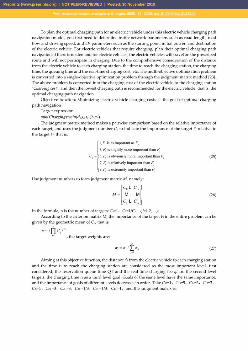
Aiming at this objective function, the distance d2 from the electric vehicle to each charging station and the time t2 to reach the charging station are considered as the most important level, first considered; the reservation queue time QT and the real-time charging fee qi’ are the second-level targets; the charging time tc as a third level goal. Goals of the same level have the same importance, and the importance of goals of different levels decreases in order. Take C12=1，C13=5，C14=3，C15=3，C23=5，C24 =3，C25 =3，C34 =1/3，C35 =1/3，C45 =1，and the judgment matrix is:



https://doi.org/10.3390/en13123208

1 1 1 15 5 3 3

1 13 3

1 13 3

1 1 5 3 31 1 5 3 3

1 3 1 1 3 1 1

M

=

(28)

After determining the target weights, the multi-objective optimization problem of charging cost is transformed into a single-objective optimization problem, and the original objective function is transformed into:

1 2 2 2 3 4 5

2 2 0.34min( ) min '

+0.349 +0.07 +0.116 +0.1169 'c T i

c T i

Charging w d w t w t w Q w qd t t Q q= + + +

→+

(29)

It can be obtained that the optimal charging path of the electric vehicle is aimed at minimizing the charging cost under the comprehensive multi-factor situation.

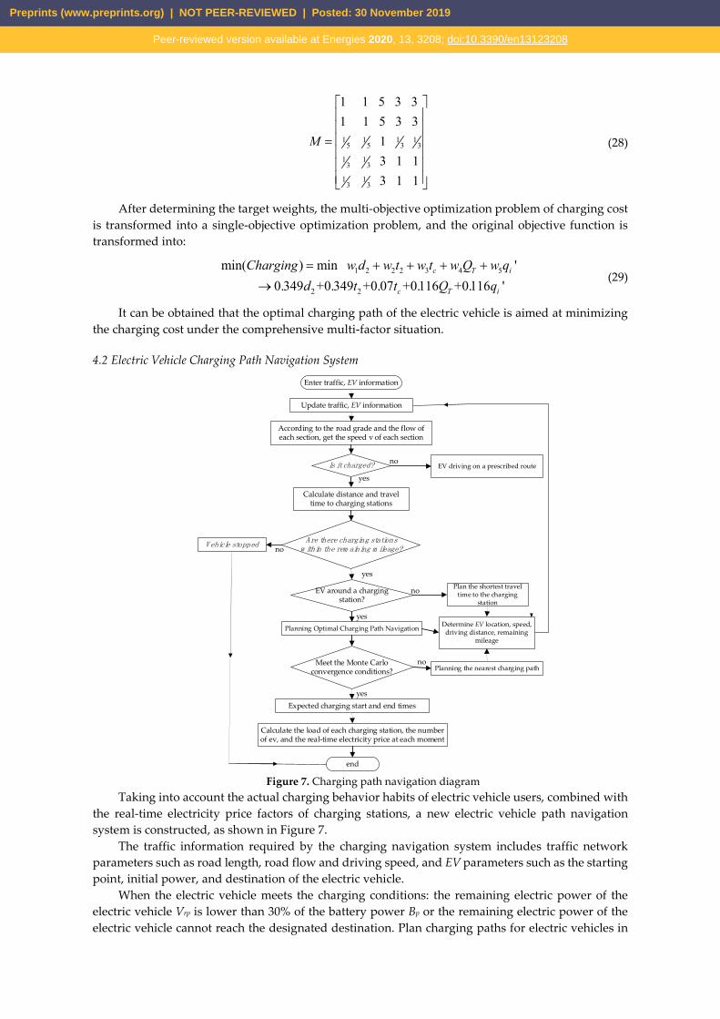
4.2 Electric Vehicle Charging Path Navigation System

According to the road grade and the flow of each section, get the speed v of each section

Enter traffic, EV information

Are there charging stations w ithin the rem aining m ileage?

Expected charging start and end times

end

yes

no

Update traffic, EV information

Calculate distance and travel time to charging stations

Planning Optimal Charging Path Navigation

Meet the Monte Carlo convergence conditions?

Vehicle stopped

Calculate the load of each charging station, the number of ev, and the real-time electricity price at each moment

yes

no

Is it charged?

EV around a charging station?

Planning the nearest charging path

Determine EV location, speed, driving distance, remaining

mileage

Plan the shortest travel time to the charging

station

yes

noEV driving on a prescribed route

yes

no

Figure 7. Charging path navigation diagram

Taking into account the actual charging behavior habits of electric vehicle users, combined with the real-time electricity price factors of charging stations, a new electric vehicle path navigation system is constructed, as shown in Figure 7.

The traffic information required by the charging navigation system includes traffic network parameters such as road length, road flow and driving speed, and EV parameters such as the starting point, initial power, and destination of the electric vehicle.

When the electric vehicle meets the charging conditions: the remaining electric power of the electric vehicle Vrp is lower than 30% of the battery power Bp or the remaining electric power of the electric vehicle cannot reach the designated destination. Plan charging paths for electric vehicles in



https://doi.org/10.3390/en13123208

turn. Electric vehicles without charging requirements are driven on the route specified in the initial simulation.

For electric vehicles that require charging, plan the charging path for each electric vehicle in order from the remaining power in ascending order. According to the Dijkstra shortest path algorithm, the travel distance and travel time from the current electric vehicle position to each charging station are calculated. First, determine whether an electric vehicle has a charging station in the driving range of its remaining power. If the electric vehicle cannot reach any charging station, the electric vehicle stops. When there is a charging station in the mileage of the electric vehicle, it is determined whether the EV is located around a charging station. Due to the actual charging behavior of electric vehicle users, if an electric vehicle is around a charging station, the charging station is the user's preferred target, then the charging path is the shortest charging path. If the electric vehicle is not obviously located near any charging station, navigate according to the optimal charging path with the goal of minimizing the charging cost of the electric vehicle to obtain the optimal charging path of the electric vehicle. If the remaining electric power of the electric vehicle cannot reach the designated charging station according to the optimal charging path navigation, then within the range of the electric vehicle's driving range, the shortest path to each charging station is the minimum value which is the recommended charging path of the electric vehicle.

5. Simulation analysis

5.1 Simulation condition setting

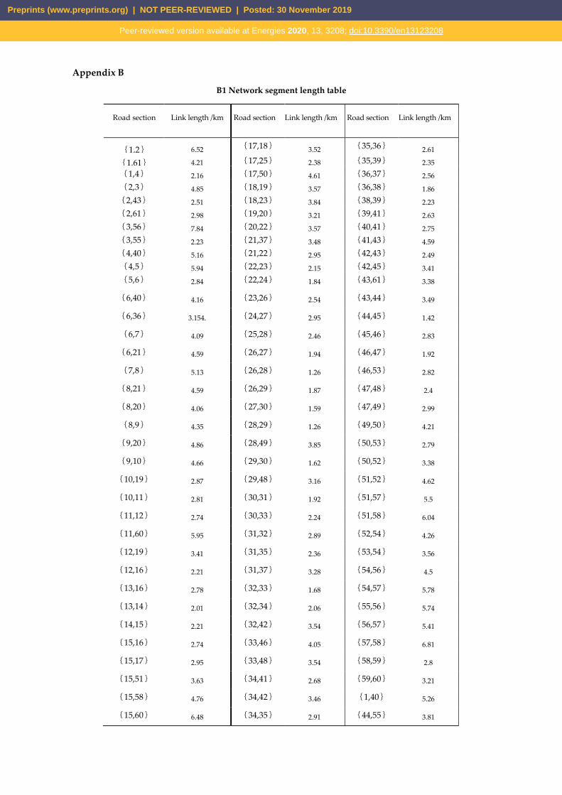
Figure 8 is a schematic diagram of traffic road levels, and the distribution of 11 charging station nodes is shown in the figure. The traffic network contains 107 roads and 61 road nodes, and the length information of each road is shown in Appendix B1. The nodes of the road traffic network and the nodes of the power distribution network are geographically coupled. For details, see the attached tables A1 and A2. This article uses Figure 9 as an example to carry out Monte Carlo simulation analysis of the electric vehicle charging path planning in this area.

In the simulation, a total of 40,000 electric vehicles were invested in the area, which was set between 6 am and 6 pm for a duration of 12 hours. Large traffic flow was introduced between 9: 00-10: 00 and 14: 00-15: 00, forming in the "double peak" traffic flow, some electric vehicles are put into use at intervals of 10 minutes.

First, determine whether the charging conditions are met based on the state of the electric vehicle that has been simulated. When the electric vehicle remaining power Vrp is lower than 30% of the battery power Bp or the electric vehicle remaining power cannot reach the designated destination, it is determined that the electric vehicle needs to perform a charging behavior and an optimal charging path is planned. If the charging conditions are not met, the electric vehicle travels on the route specified in the initial simulation, and the remaining power changes with time and changes according to the amount of power consumption. If the electric vehicle is around a certain charging station, plan to charge the electric vehicle to the current charging station location. For example, when an electric vehicle is not near any charging station, its optimal path is planned by the optimal charging path navigation. If the electric vehicle cannot reach the optimal charging station location, plan the nearest charging path.



https://doi.org/10.3390/en13123208

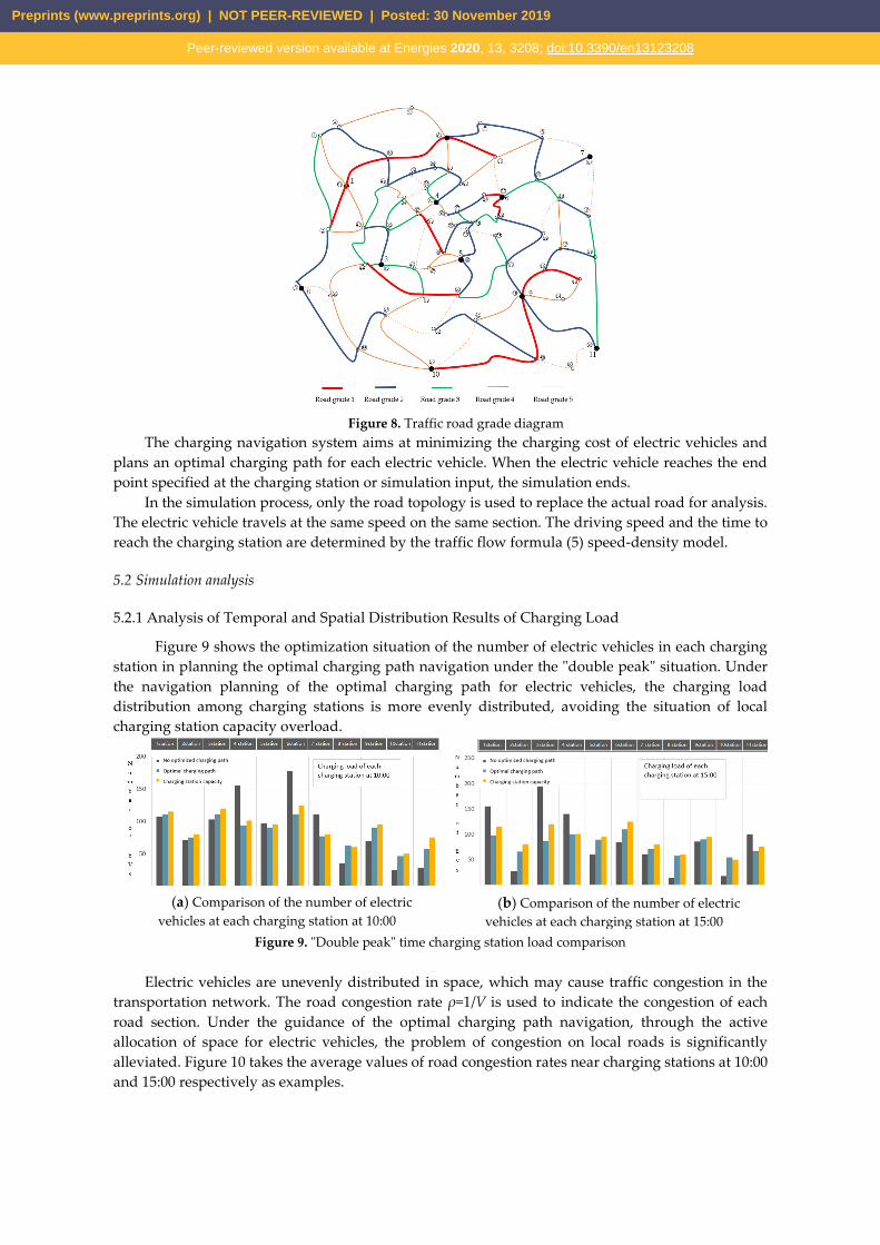
Figure 8. Traffic road grade diagram

The charging navigation system aims at minimizing the charging cost of electric vehicles and plans an optimal charging path for each electric vehicle. When the electric vehicle reaches the end point specified at the charging station or simulation input, the simulation ends.

In the simulation process, only the road topology is used to replace the actual road for analysis. The electric vehicle travels at the same speed on the same section. The driving speed and the time to reach the charging station are determined by the traffic flow formula (5) speed-density model.

5.2 Simulation analysis

5.2.1 Analysis of Temporal and Spatial Distribution Results of Charging Load

Figure 9 shows the optimization situation of the number of electric vehicles in each charging station in planning the optimal charging path navigation under the "double peak" situation. Under the navigation planning of the optimal charging path for electric vehicles, the charging load distribution among charging stations is more evenly distributed, avoiding the situation of local charging station capacity overload.

(a) Comparison of the number of electric

vehicles at each charging station at 10:00

(b) Comparison of the number of electric

vehicles at each charging station at 15:00 Figure 9. "Double peak" time charging station load comparison

Electric vehicles are unevenly distributed in space, which may cause traffic congestion in the

transportation network. The road congestion rate ρ=1/V is used to indicate the congestion of each road section. Under the guidance of the optimal charging path navigation, through the active allocation of space for electric vehicles, the problem of congestion on local roads is significantly alleviated. Figure 10 takes the average values of road congestion rates near charging stations at 10:00 and 15:00 respectively as examples.



https://doi.org/10.3390/en13123208

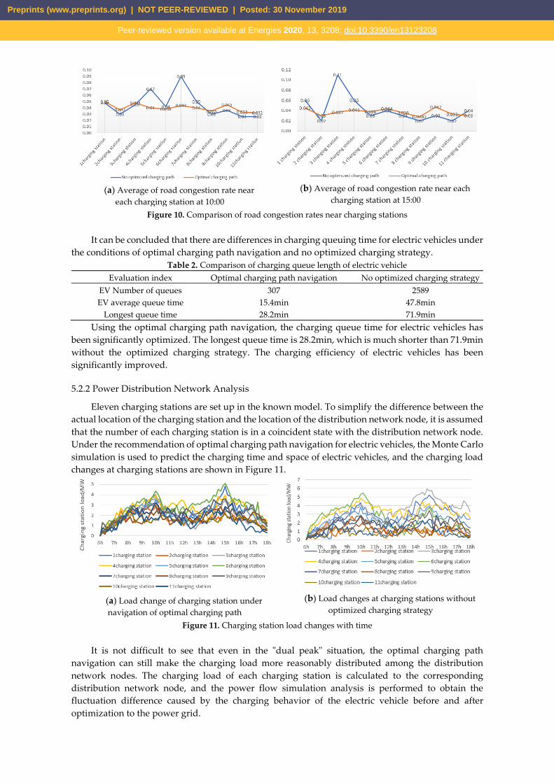
(a) Average of road congestion rate near

each charging station at 10:00

(b) Average of road congestion rate near each

charging station at 15:00 Figure 10. Comparison of road congestion rates near charging stations

It can be concluded that there are differences in charging queuing time for electric vehicles under

the conditions of optimal charging path navigation and no optimized charging strategy. Table 2. Comparison of charging queue length of electric vehicle

Evaluation index Optimal charging path navigation No optimized charging strategy EV Number of queues 307 2589 EV average queue time 15.4min 47.8min

Longest queue time 28.2min 71.9min Using the optimal charging path navigation, the charging queue time for electric vehicles has

been significantly optimized. The longest queue time is 28.2min, which is much shorter than 71.9min without the optimized charging strategy. The charging efficiency of electric vehicles has been significantly improved.

5.2.2 Power Distribution Network Analysis

Eleven charging stations are set up in the known model. To simplify the difference between the actual location of the charging station and the location of the distribution network node, it is assumed that the number of each charging station is in a coincident state with the distribution network node. Under the recommendation of optimal charging path navigation for electric vehicles, the Monte Carlo simulation is used to predict the charging time and space of electric vehicles, and the charging load changes at charging stations are shown in Figure 11.

(a) Load change of charging station under navigation of optimal charging path

(b) Load changes at charging stations without

optimized charging strategy Figure 11. Charging station load changes with time

It is not difficult to see that even in the "dual peak" situation, the optimal charging path

navigation can still make the charging load more reasonably distributed among the distribution network nodes. The charging load of each charging station is calculated to the corresponding distribution network node, and the power flow simulation analysis is performed to obtain the fluctuation difference caused by the charging behavior of the electric vehicle before and after optimization to the power grid.



https://doi.org/10.3390/en13123208

(a) 30-node distribution network voltage under the

optimal charging path navigation

(b) Voltage of 30-node distribution network

without optimized charging strategy

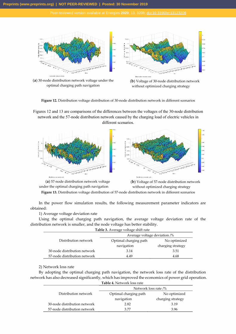
Figure 12. Distribution voltage distribution of 30-node distribution network in different scenarios

Figures 12 and 13 are comparisons of the differences between the voltages of the 30-node distribution network and the 57-node distribution network caused by the charging load of electric vehicles in

different scenarios.

(a) 57-node distribution network voltage

under the optimal charging path navigation

(b) Voltage of 57-node distribution network

without optimized charging strategy Figure 13. Distribution voltage distribution of 57-node distribution network in different scenarios

In the power flow simulation results, the following measurement parameter indicators are

obtained: 1) Average voltage deviation rate Using the optimal charging path navigation, the average voltage deviation rate of the

distribution network is smaller, and the node voltage has better stability. Table 3. Average voltage shift rate

Distribution network Average voltage deviation /%

Optimal charging path navigation

No optimized charging strategy

30-node distribution network 3.14 3.51 57-node distribution network 4.49 4.68

2) Network loss rate By adopting the optimal charging path navigation, the network loss rate of the distribution

network has also decreased significantly, which has improved the economics of power grid operation. Table 4. Network loss rate

Distribution network Network loss rate /%






https://doi.org/10.3390/en13123208

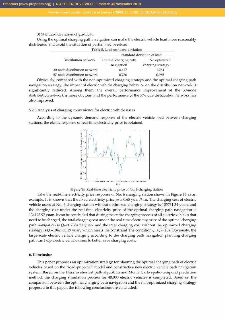
3) Standard deviation of grid load Using the optimal charging path navigation can make the electric vehicle load more reasonably

distributed and avoid the situation of partial load overload. Table 5. Load standard deviation

Distribution network Standard deviation of load




Obviously, compared with the non-optimized charging strategy and the optimal charging path navigation strategy, the impact of electric vehicle charging behavior on the distribution network is significantly reduced. Among them, the overall performance improvement of the 30-node distribution network is more obvious, and the performance of the 57-node distribution network has also improved.

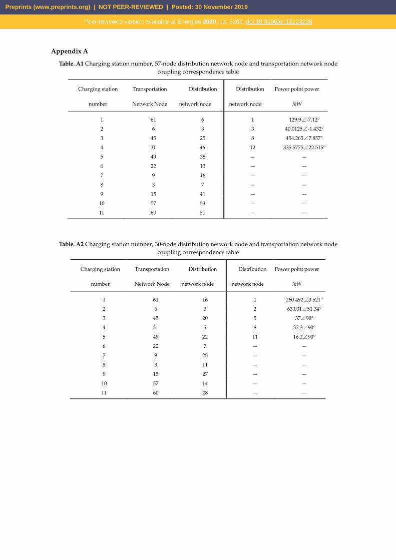
5.2.3 Analysis of charging convenience for electric vehicle users

According to the dynamic demand response of the electric vehicle load between charging stations, the elastic response of real-time electricity price is obtained.

Figure 14. Real-time electricity price of No. 6 charging station

Take the real-time electricity price response of No. 6 charging station shown in Figure 14 as an example. It is known that the fixed electricity price p0 is 0.65 yuan/kwh. The charging cost of electric vehicle users at No. 6 charging station without optimized charging strategy is 105731.34 yuan, and the charging cost under the real-time electricity price of the optimal charging path navigation is 134193.97 yuan. It can be concluded that during the entire charging process of all electric vehicles that need to be charged, the total charging cost under the real-time electricity price of the optimal charging path navigation is Q1=917304.71 yuan, and the total charging cost without the optimized charging strategy is Q0=1042968.19 yuan, which meets the constraint The condition Q1<Q0 (18). Obviously, the large-scale electric vehicle charging according to the charging path navigation planning charging path can help electric vehicle users to better save charging costs.

6. Conclusion

This paper proposes an optimization strategy for planning the optimal charging path of electric vehicles based on the "road-price-net" model and constructs a new electric vehicle path navigation system. Based on the Dijkstra shortest path algorithm and Monte Carlo spatio-temporal prediction method, the charging simulation process for 40,000 electric vehicles is completed. Based on the comparison between the optimal charging path navigation and the non-optimized charging strategy proposed in this paper, the following conclusions are concluded:



https://doi.org/10.3390/en13123208

1) Adopting the optimal charging path navigation, you can more rationally plan the charging load between charging stations, avoid the phenomenon of partial load overload at the charging stations as much as possible, effectively improve the charging efficiency of electric vehicles, and greatly reduce electric vehicles. The length of the charging queue has certain reference value for the expansion and capacity adjustment of the charging station.

2) In the simulation of the "double peak" phenomenon of real traffic, this article adopts the optimal charging path navigation method, which can effectively alleviate the local traffic congestion caused by the accumulation of more electric vehicles at a charging station and improve the entire traffic. The running status of the network.

3) Compared with the non-optimized charging strategy, the average voltage offset rate, network loss rate, and standard deviation of the grid load are significantly reduced when the optimal charging path is adopted for navigation, and the overall operating capacity of the distribution network It has been improved, and the impact of the charging behavior of electric vehicles on the entire distribution network has been minimized.

4) Adopting the optimal charging path navigation, from the perspective of the immediate interests of electric vehicle users, it can more reasonably save charging costs for electric vehicle users.

In the simulation of this paper, certain assumptions are made on the types of electric vehicles, charging paths, and actual traffic conditions. Based on the existing "car-net-road" model and the concept of the spatio-temporal prediction of the charging load of electric vehicles, the impact of real-time electricity prices on the selection of electric vehicle charging paths was initially discussed in order to establish a more comprehensive electric vehicle based on the consideration of charging users. Car charging path navigation system. Therefore, in the future, the planning of electric vehicle charging paths will be comprehensively considered from the distribution of charging facilities, capacity allocation, and road traffic simulation.

7. Patents

CN110388932A --- Electric vehicle charging navigation method Author Contributions: All authors contributed to the research in this paper. Z.W. and .W. conceived and

designed the model. X.F. and P.M. provided the data. W.Y. analyzed the data. Z.D. and Z.Y. wrote the paper.

Funding: This work is supported by the National Natural Science Foundation of China (grant no. 51477099); Open Project Foundation of Key Laboratory of Control of Power Transmission and Conversion (SJTU), Ministry of Education (grant no.2016AB14).

Conflicts of Interest: The authors declare no conflict of interest.



https://doi.org/10.3390/en13123208

Appendix A

Table. A1 Charging station number, 57-node distribution network node and transportation network node coupling correspondence table

Table. A2 Charging station number, 30-node distribution network node and transportation network node

coupling correspondence table

Charging station

number

Transportation

Network Node

Distribution

network node

Distribution

network node

Power point power

/kW

1 61 6 1 129.9∠-7.12°

2 6 3 3 40.0125∠-1.432°

3 45 25 8 454.265∠7.857°

4 31 46 12 335.5775∠22.515°

5 49 38 — —

6 22 13 — —

7 9 16 — —

8 3 7 — —

9 15 41 — —

10 57 53 — —

11 60 51 — —

Charging station

number

Transportation

Network Node

Distribution

network node

Distribution

network node

Power point power

/kW

1 61 16 1 260.492∠3.521°

2 6 3 2 63.031∠51.34°

3 45 20 5 37∠90°

4 31 5 8 37.3∠90°

5 49 22 11 16.2∠90°

6 22 7 — —

7 9 25 — —

8 3 11 — —

9 15 27 — —

10 57 14 — —

11 60 28 — —



https://doi.org/10.3390/en13123208

Appendix B

B1 Network segment length table

Road section Link length /km Road section Link length /km Road section Link length /km

｛1,2｝ 6.52 ｛17,18｝ 3.52 ｛35,36｝ 2.61

｛1,61｝ 4.21 ｛17,25｝ 2.38 ｛35,39｝ 2.35 ｛1,4｝ 2.16 ｛17,50｝ 4.61 ｛36,37｝ 2.56 ｛2,3｝ 4.85 ｛18,19｝ 3.57 ｛36,38｝ 1.86 ｛2,43｝ 2.51 ｛18,23｝ 3.84 ｛38,39｝ 2.23 ｛2,61｝ 2.98 ｛19,20｝ 3.21 ｛39,41｝ 2.63 ｛3,56｝ 7.84 ｛20,22｝ 3.57 ｛40,41｝ 2.75 ｛3,55｝ 2.23 ｛21,37｝ 3.48 ｛41,43｝ 4.59 ｛4,40｝ 5.16 ｛21,22｝ 2.95 ｛42,43｝ 2.49 ｛4,5｝ 5.94 ｛22,23｝ 2.15 ｛42,45｝ 3.41 ｛5,6｝ 2.84 ｛22,24｝ 1.84 ｛43,61｝ 3.38

｛6,40｝ 4.16 ｛23,26｝ 2.54 ｛43,44｝ 3.49

｛6,36｝ 3.154. ｛24,27｝ 2.95 ｛44,45｝ 1.42

｛6,7｝ 4.09 ｛25,28｝ 2.46 ｛45,46｝ 2.83

｛6,21｝ 4.59 ｛26,27｝ 1.94 ｛46,47｝ 1.92

｛7,8｝ 5.13 ｛26,28｝ 1.26 ｛46,53｝ 2.82

｛8,21｝ 4.59 ｛26,29｝ 1.87 ｛47,48｝ 2.4

｛8,20｝ 4.06 ｛27,30｝ 1.59 ｛47,49｝ 2.99

｛8,9｝ 4.35 ｛28,29｝ 1.26 ｛49,50｝ 4.21

｛9,20｝ 4.86 ｛28,49｝ 3.85 ｛50,53｝ 2.79

｛9,10｝ 4.66 ｛29,30｝ 1.62 ｛50,52｝ 3.38

｛10,19｝ 2.87 ｛29,48｝ 3.16 ｛51,52｝ 4.62

｛10,11｝ 2.81 ｛30,31｝ 1.92 ｛51,57｝ 5.5

｛11,12｝ 2.74 ｛30,33｝ 2.24 ｛51,58｝ 6.04

｛11,60｝ 5.95 ｛31,32｝ 2.89 ｛52,54｝ 4.26

｛12,19｝ 3.41 ｛31,35｝ 2.36 ｛53,54｝ 3.56

｛12,16｝ 2.21 ｛31,37｝ 3.28 ｛54,56｝ 4.5

｛13,16｝ 2.78 ｛32,33｝ 1.68 ｛54,57｝ 5.78

｛13,14｝ 2.01 ｛32,34｝ 2.06 ｛55,56｝ 5.74

｛14,15｝ 2.21 ｛32,42｝ 3.54 ｛56,57｝ 5.41

｛15,16｝ 2.74 ｛33,46｝ 4.05 ｛57,58｝ 6.81

｛15,17｝ 2.95 ｛33,48｝ 3.54 ｛58,59｝ 2.8

｛15,51｝ 3.63 ｛34,41｝ 2.68 ｛59,60｝ 3.21

｛15,58｝ 4.76 ｛34,42｝ 3.46 ｛1,40｝ 5.26

｛15,60｝ 6.48 ｛34,35｝ 2.91 ｛44,55｝ 3.81



https://doi.org/10.3390/en13123208

References

1. Yang, X.L. The development trend and foreground of the electric vehicle[J]. Auto Mobile Science & Technology, 2007(6):10-13(in Chinese).

2. Sun, P.C. The current situation and development trend of the electric vehicle[J]. Scientific Chinese, 2006(8):44-47(in Chinese).

3. uang, S.F. Research on armonic Problems of Electric Vehicle Charger (Station) [D]. Beijing: Beijing Jiaotong University, 2008.

4. Lu. Y.X.; Zhang, X.M.; Pu, X.W. armonic study of electric vehicle chargers[J] . Proceedings of the Chinese Society of Universities, 2006, 18(3): 51-54(in Chinese).

5. Gao, C.W.; Zhang, L. A survey of influence of electric vehicle charging on power grid[J]. Power System Technology.2011, 35(2):127-131(in Chinese).

6. uang, R. Impacts of electric vehicles charging on the load of power system[D]. Shanghai: Shanghai Jiao Tong University, 2012(in Chinese).

7. u, Z.C.; Song, Y..; Xu. Z.W. Impacts and utilization of electric vehicles integration into power systems[J]. Proceedings of the CSEE, 2012, 32(4): 1-10(in Chinese).

8. Shao, Y.C.; Mu, Y.F.; Yu, X.D.; Dong, X..; Jia, .J.; Wu, J.Z.; Zeng, W. A Spatial-temporal Charging Load Forecast and Impact Analysis Method for Distribution Network Using EVs-Traffic-Distribution Model[J]. Proceedings of the CSEE, 2017, 37(18): 5207-5219+5519 (in Chinese).

9. Wu, K..; Wang J.Y.; Li, W.; Zhu, Y.Y. Research on Operation Mode of New Generation Power System for Energy Internet[J]. Proceedings of the CSEE, 2019, 39(04): 966-979(in Chinese).

10. Zhu, F.L. Research on Evaluation Index System of Urban Road Traffic Congestion[D]. Nanjing: Southeast University, 2006: 6.

11. Yuichi Kobayashi, Noboru Kiyama, irokazu Aoshima , et al. A Route Search Method for Electric Vehicles in Consideration of Range and Locations of Charging Stations[C]. Baden-Baden: 2011 IEEE Intelligent Vehicles Symposium: IV, 2011: 6.

12. Su, S.; Yang, L.; Li, Y.X.; Luo, W.; Wang, S.D.; e, L.B. Electric vehicle charging path planning considering real-time dynamic energy consumption[J]. Automation of Electric Power Systems, 2019, 43(07): 136-147.

13. Luo, Y.G.; Yan, Y.Y.; Zhu, T. Intelligent electric vehicle optimal charging path planning method[J]. Engineering Research: Engineering in an Interdisciplinary Perspective, 2014, 6(1): 92-98.

14. Yan, Y.Y.; Luo, Y.G.; Zhu, T.; et al. Optimal charging route recommendation method based on transportation and distribution information[J]. Proceedings of the CSEE, 2015, 35(2): 310-318(in Chinese).

15. Wan, S. Electric vehicle charging/changing scheduling for traffic and power grid comprehensive optimization[D]. Beijing Forestry University, 2015.

16. Su, S.; Sun, J.W.; Lin, X.N.; Li, X.S. Electric car smart charging navigation[J]. Proceedings of the CSEE, 2013, 33(S1): 59-67(in Chinese).

17. TRB Committee, America. ighway Capacity Manual[M] . U.S. Department of Transportation, Federal ighway Administration , 1986: 38.

18. Chen, S. Research on practical velocity-volume model of urban street[D]. Nanjing: Southeast University, 2004.

19. Xiao, Z.G. Evaluation of Regional OD Matrix Inversion Technology and Its Theoretical Research[D]. uazhong University of Science and Technology, 2006.

20. Li, Y. Customer Satisfaction Index Model and Its Evaluation Method [D]. China University of Mining and Technology (Beijing), 2008.

21. Liu, C.; Feng, D..; Fang, C. A new pricing method for multi-solution of electricity price in real-time market [J/OL]. Proceedings of the CSEE: 1-14[2019-06-12] (in Chinese).

22. Bai, G.P. Research on large-scale construction and grid adaptability of electric vehicle charging (discharging) power station [D]. Beijing: Beijing Jiaotong University, 2011: 26.

23. Lu, T.; Tang, Y.; Cong, P.W.; Bo, B. Multi-objective coordination planning of distributed power supply and distribution network frame[J]. Automation of Electric Power Systems, 2013, 37(21): 139-145.



https://doi.org/10.3390/en13123208

article optimization strategy of electric vehicles

Documents