artificial neural network model for the determination of gsm … · full length article artiﬁcial...

Engineering Science and Technology, an International Journal xxx (2016) xxx–xxx

Contents lists available at ScienceDirect

Engineering Science and Technology,an International Journal

journal homepage: www.elsevier .com/ locate / jestch

Full Length Article

Artificial Neural Network model for the determination of GSM Rxlevelfrom atmospheric parameters

http://dx.doi.org/10.1016/j.jestch.2016.11.0022215-0986/� 2016 Karabuk University. Publishing services by Elsevier B.V.This is an open access article under the CC BY-NC-ND license (http://creativecommons.org/licenses/by-nc-nd/4.0/).

⇑ Corresponding author.E-mail addresses: [email protected] (J.O. Eichie), onyedidavid@

futminna.edu.ng (O.D. Oyedum), [email protected] (M.O. Ajewole),[email protected] (A.M. Aibinu).

Peer review under responsibility of Karabuk University.

Please cite this article in press as: J.O. Eichie et al., Artificial Neural Network model for the determination of GSM Rxlevel from atmospheric paraEng. Sci. Tech., Int. J. (2016), http://dx.doi.org/10.1016/j.jestch.2016.11.002

Eichie Julia Ofure a,⇑, Oyedum Onyedi David a, Ajewole Moses Oludare b, Aibinu Abiodun Musa c

aDepartment of Physics, Federal University of Technology, Minna, NigeriabDepartment of Physics, Federal University of Technology, Akure, NigeriacDepartment of Mechatronics Engineering, Federal University of Technology, Minna, Nigeria

a r t i c l e i n f o a b s t r a c t

Article history:Received 2 August 2016Revised 25 October 2016Accepted 3 November 2016Available online xxxx

Keywords:Artificial Neural NetworkDew pointRelative humidityRxlevelTemperature

Accurate received signal level (Rxlevel) values are useful for mobile telecommunication network plan-ning. Rxlevel is affected by the dynamics of the atmosphere through which it propagates. Adequateknowledge of the prevailing atmospheric conditions in an environment is essential for proper networkplanning. However most of the existing GSM received signal determination model are function of dis-tance between point of signal reception and transmitting site thus necessitating the development of amodel that involve the use of atmospheric parameters in the determination of received GSM signal level.In this paper, a three stage approach was used in the development of the model using some atmosphericparameters such as atmospheric temperature, relative humidity and dew point. The selected and easilymeasurable atmospheric parameters were used as input parameters in developing two new models forcomputing the Rxlevel of GSM signal using a three-step approach. Data acquisition and pre-processingserves as the first stage and formulation of ANN design and the development of parametric model forthe Rxlevel using ANN synaptic weights form the second stage of the proposed approach. The third stageinvolves the use of ANN weight and bias values, and network architecture in the development of themodel equation. In evaluating the performance of the proposed models, network parameters were variedand the results obtained using mean squared error (MSE) as performance measure showed the developedmodel with 33 neurons in the hidden layer and tansig activation, function in both the hidden and outputlayers as the optimal model with least MSE value of 0.056. Thus showing that the developed model has anacceptable accuracy value as demonstrated from comparison of results with actual measured values.� 2016 Karabuk University. Publishing services by Elsevier B.V. This is an open access article under the CC

BY-NC-ND license (http://creativecommons.org/licenses/by-nc-nd/4.0/).

1. Introduction

Empirical models are used in the planning of mobile communi-cation networks. Due to the differences in environmental struc-tures, local terrain profiles and weather conditions, the signalstrength and path loss prediction model for a given environment,with reference to existing empirical models, often differ from theoptimal model. Accurate signal strength values are necessary fornetwork planning. Mobile telecommunications depend on thepropagation of radio waves within the troposphere, the region ofthe atmosphere extending from the Earth’s surface up to an alti-tude of about 16 km at the equator or 8 km at the poles [1]. Prop-

agation of radio waves through space is governed to a great degreeby the dynamics and physical properties of the atmosphere andobjects in the propagation path. Environmental, atmospheric andclimatic conditions impair Global System for Mobile Communica-tion (GSM) signal propagation and may result in reduction of thestrength of received signal and deformation of signal quality overtime. The environmental and weather effects on signal strengthneed to be properly understood in given environments to enhanceoptimal planning of such networks.

The Earth’s weather system is confined to the troposphere andthe fluctuations in weather parameters like temperature, pressureand humidity within the atmospheric layer cause the refractiveindex of the air in this layer to vary from one location to anotherand from time to time. The variation in the refractive index ofthe atmosphere results in various degrees of refraction of mobilesignals. Under abnormal conditions such as ducting, the signalstrength can also be enhanced and this enables the signals to reachunintended locations where they may constitute interference to

meters,

http://creativecommons.org/licenses/by-nc-nd/4.0/

http://dx.doi.org/10.1016/j.jestch.2016.11.002

http://creativecommons.org/licenses/by-nc-nd/4.0/

mailto:[email protected]

mailto:onyedidavid@ futminna.edu.ng

mailto:onyedidavid@ futminna.edu.ng

mailto:[email protected]

mailto: [email protected]


http://www.sciencedirect.com/science/journal/22150986

http://www.elsevier.com/locate/jestch


2 J.O. Eichie et al. / Engineering Science and Technology, an International Journal xxx (2016) xxx–xxx

other co-channel networks. The refractive properties of the tropo-sphere is expressed by the radio refractivity, N, given by

N ¼ ðn� 1Þ � 106 ð1Þwhere n = refractive index of air. N depends on meteorological fac-tors of air pressure, P (hPa), air temperature, t (�C) and water vapourpressure, e (hPa), which are related to N as [2]:

N ¼ 77:6PT

� �þ 3:732� 105 e

T2

� �ð2Þ

where T(K) = t + 273, and

e ¼ Hes100

ð3Þ

where e is water vapour pressure, H is relative humidity, and es thesaturated water vapour pressure given as:

es ¼ 6:11exp17:502t

T

� �ð4Þ

Surface refractivity, Ns, is known to have high correlation withradio field strength values [3,4] and seasonal variations in Ns havebeen found to agree in general with the observations of the varia-tion of radio field strength at VHF and UHF in Nigeria [5,6]. Thus,surface radio refractivity is a function of atmospheric parametersof temperature, pressure and relative humidity near the surface.

Temperature and relative humidity have been found to havesome correlation with GSM Rxlevel [7,8,9]. Zilinskas et al. [10]showed that there is no obvious correlation between atmosphericpressure and received signal strength. Some relationships existbetween atmospheric temperature, relative humidity and dewpoint. Atmospheric temperature is the degree of hotness or cold-ness of the atmosphere. Humidity is a measure of the quantity ofwater vapour or the gaseous state of water, in the atmosphere,and is usually invisible. The maximum amount of water vapourin the atmosphere depends on the atmospheric temperature [9].Relative humidity (RH) defines the amount of water vapour inthe atmosphere relative to the maximum amount of water vapourthe air can take at the same atmospheric temperature and pres-sure. Relative humidity of the saturated atmosphere is 100% andas atmospheric water vapour increases towards saturation point,atmospheric temperature decreases. In other words, relativehumidity is inversely proportional to atmospheric temperature.Dew point is the temperature to which the atmosphere must becooled to enable water vapour condense into liquid water or ice(RH = 100%). Relative humidity and dew point are both reflectionof the amount of water vapour in the atmosphere. Each of themis also a function of temperature. Thus, relative humidity, temper-ature and dew point are interrelated and their relationship withradio field strength makes them reliable as inputs in received sig-nal level computation model. Artificial Neural Network has beenfound to be very effective in prediction problems and useful inthe development of models [11].

Artificial Neural Network (ANN) is one of the artificial intelli-gence techniques. It is based on understanding the structure andfunction of the physical biological neurons of the human brainand the ability of the human brain to learn through example[12]. ANN has proven to be flexible and with capability to learnthe underlying relationships between the inputs and outputs of aprocess, without needing the explicit knowledge of how these vari-ables are related [13]. ANN can learn, adapt, predict and classify. Inthis study, the atmospheric parameters such as temperature, rela-tive humidity and dew point that have been found to have rela-tionship with the temporal variation of GSM Rxlevel were usedto develop a model that computes GSM Rxlevel. This is useful fordetermining coverage areas of base stations, frequency assign-

Please cite this article in press as: J.O. Eichie et al., Artificial Neural Network mEng. Sci. Tech., Int. J. (2016), http://dx.doi.org/10.1016/j.jestch.2016.11.002

ments, interference analysis, handover optimisation, optimaltransmitting antenna height and power level adjustment.

There is need for the determination of propagation characteris-tics of given environments, especially in tropical regions of Africa,as requested by ITU-R. Acquisition of empirical signal field strengthdata could be difficult, due to paucity of relevant equipment. Butacquisition of atmospheric data is relatively cheaper and the dataare more available.

The rest of this paper is organized as follows: Section 2 presentsliterature review while Section 3 presents model design and devel-opment. Results and discussion is presented in Section 4 whileconclusion is in Section 5.

2. Literature review

This section is divided into two sub-sections. In subsection 2.1,review of recently published related work from literature havebeen undertaken while in subsection 2.2 an overview into ANNwhich is used in Section 3 in the developing of the appropriatemodel has been provided.

2.1. Related field Measurements and ANN Applications

Adewumi et al. [8] studied the influence of atmosphericparameters on UHF Radio Propagation in South Western Nigeria.Received signal level was observed to increase with increase intemperature while relative humidity increased with signal pathloss. The study revealed that air temperature and relative humid-ity have significant influence on UHF signal propagation withinthe tropospheric region of southwest Nigeria. Zilinskas et al.[10] investigated the influence of atmospheric radio refractivityon WiMax signal level. The study revealed that atmospheric radiorefractivity, as a combination of temperature and relative humid-ity, has impact on the variation of received signal level. Increasein refractivity values had a corresponding decrease in receivedsignal level.

Famorji et al. [14] revealed an inverse relationship betweenatmospheric radio refractivity and UHF received signal level withcorrelation coefficient value of �0.97. The study also revealed adirect relationship between atmospheric radio refractivity and rel-ative humidity and an inverse relationship between atmosphericradio refractivity and temperature. Sheowu and Akinyemi [15]investigated the effect of climatic change on GSM signal propaga-tion by sampling the three ITU regions in Nigeria at different cli-matic seasons of rain (May–June) and harmattan (November–March). The result obtained revealed that climate affects signalpropagation.

Afrand et al. [16] developed an optimal Artificial Neural Net-work to predict the thermal conductivity ratio of the magneticnanofluid and Afrand et al. [17] predicted dynamic viscosity of ahybrid nano-lubricant using an optimal Artificial Neural Network.Comparison of the experimental data, empirical correlation andthe optimal ANN outputs showed that the optimal Artificial NeuralNetwork model is more accurate. Philippopoulos and Deligiorgi[18] assessed the spatial predictive ability of ANNs to estimatemean hourly wind speed values in Chania City, Greece. The pre-dicted values were compared with five traditional spatial interpo-lation schemes and ANNs were observed to efficiently predict themean wind speed spatial variability in Chania City.

Esfe et al. [19] applied feedforward multilayer perceptron Arti-ficial Neural Networks and empirical correlation, for the predictionof thermal conductivity of Mg(OH)2–EG using experimental data.The results of the developed models revealed that, in the absenceof costly and time-consuming tests, the impact of temperatureand volume fraction on Mg(OH)2–EG nanofluids’ thermal

odel for the determination of GSM Rxlevel from atmospheric parameters,


J.O. Eichie et al. / Engineering Science and Technology, an International Journal xxx (2016) xxx–xxx 3

conductivity can be analyzed with ANN models. Litta et al. [20]evaluated the utility of multilayer perceptron network (MLPN)ANN model for the prediction of hourly surface temperature andrelative humidity in Kolkata, India. The study showed that ANNmodels were capable of predicting hourly temperature and relativehumidity adequately and the developed ANN models were appliedin the prediction of thunderstorm in Kolkata.

2.2. Overview of ANN

ANN is an information processing system constituted by anassembly of a large number of simple processing elements thatare interconnected to perform a parallel distributed processing inorder to solve specific task, such as pattern classification, functionapproximation, clustering (or categorisation), prediction (forecast-ing or estimation), optimisation and control [13]. The Process Ele-ments (PEs) attempt to simulate the structure and function of thephysical biological neurons of the human brain. The fundamentalprinciple of ANN is based on finding coefficients between theinputs and outputs of a problem, making connections betweeninput and output layers and performing operations on a learningsystem [21]. The fundamental element of ANN is the neuron. Eachneuron handles:

i. the multiplication of the network inputs, x1, x2, x3, . . .xn(from original data, or from the output of other neurons ina neural network) by the associated input weights,

ii. the summation of the weight and input product to the biasvalue associated with the neuron, and

iii. the passage of the summation result, u, through a linear ornonlinear transformation called the activation function, u.The neuron’s output, y, is the result of the action of the acti-vation function.

PleaseEng. S

u ¼ f ðuÞ ð5Þ
!
y ¼ uXni¼1

xiwi þ b ð6Þ

� �
y ¼ u wTxþ b ð7Þ
where b is the bias value (or external threshold), wi, is theweight of the respective inputs xi, u is the argument of theactivation function and wT is a transpose of the weight vector.

Fig. 1. Artificia

cite this article in press as: J.O. Eichie et al., Artificial Neural Network mci. Tech., Int. J. (2016), http://dx.doi.org/10.1016/j.jestch.2016.11.002

The weight and bias are adjustable parameters of the neuronthat causes the network to exhibit some desired or interestingbehaviours. Fig. 1 shows an illustration of an artificial neuron.

ANN architecture can be classified into two main topologies:feed-forward multilayer networks and feedback recurrent net-works. In the former network, feedback connections are notallowed while loops and iteration for a potentially long time beforeproducing a response exist in the latter. The most commonly usedtype of feed-forward network is the multilayer perceptron [22]. Amultilayer perceptron (MLP) network consists of a set of inputnodes, one or more hidden layers and a set of output nodes inthe output layer. MLP network has the ability to model simpleand as well as complicated functional relationships.

3. Model design and development

In this section, the design and development of the ANNmodel fordetermination of Rxlevel is presented. The proposed approachinvolves a three stage approach namely, data collection and pre-processing, network design andmodel development. Detailed infor-mation about each of the aforementioned stages is providedherewith.

3.1. Data collection and pre-processing

Twelve months (June 2014 to May 2015) atmospheric data wereacquired from the Nigeria Environmental and Climate ObservationProgramme (NECOP) weather station at the Bosso Campus of theFederal University of Technology, Minna, Nigeria. Concurrently,the GSM Rxlevel of Mobile Telecommunications Network (MTN)with the frequency band 1835–1850 MHz was measured using aspectrum analyser (SPECTRAN HF 6065) connected to a laptoploaded with Aarisona data logging software. Figs. 2 and 3 showthe NECOP weather station and the GSM Rxlevel measurementsetup used in this study.

The atmospheric data and GSM Rxlevel were measured at 5 minand 500 ms intervals respectively, GSM Rxlevel data were averagedto 5 min intervals for each day of the 12 months. The missing datain the input data (atmospheric temperature, relative humidity anddew point data) and the output data (GSM Rxlevel data) werereplaced by the average of neighbouring values. The terrain ofthe propagation environment is relatively flat and unpaved. Thereare farm lands, vegetation cover, few trees and bungalow buildingsbetween the transmitting and the measurement sites. The physicalprofile of the fixed wireless link consisting of the MTN base stationand the measurement site is shown in Fig. 4.

l Neuron.



(a) A view of the Weather Station (b) Downloading of Atmospheric Data to a laptop

Fig. 2. The NECOP Weather Station.

Laptop

Antenna

Spectrum Analyser

Pistol Grip Stand

Fig. 3. Spectran HF 6065 and a Laptop for Data Logging.

Measurement Site

MTN BTS

300 m

Fig. 4. Physical Profile of the Fixed Wireless Link (Google Earth).


Please cite this article in press as: J.O. Eichie et al., Artificial Neural Network model for the determination of GSM Rxlevel from atmospheric parameters,Eng. Sci. Tech., Int. J. (2016), http://dx.doi.org/10.1016/j.jestch.2016.11.002



3.2. Design of ANN based Rxlevel determination model

The proposed MLP network consists of 3 nodes at the inputlayer, one hidden layer and 1 node at the output layer. In the pro-posed model, 3 most frequently used activation functions havebeen considered [23]. These are:

i. Logistic sigmoid activation function also known as logsig.

f ðuÞ ¼ 11þ e�u

ð8Þ

ii. Hyperbolic tangent sigmoid activation function also knownas tansig.

f ðuÞ ¼ 21þ e�2u � 1 ð9Þ

iii. Linear activation function also known as purelin.

f ðuÞ ¼ u ð10ÞA schematic of the proposed MLP network with variable neurons inthe hidden layer is shown in Fig. 5.where xi (where 1 6 iP 3) arethe set of inputs; wij and wjk are adjustable weight values: wij con-nects the ith input to the jth neuron in the hidden layer, wjk con-nects the jth output in the hidden layer to the kth node in theoutput layer; yk (where k = l) is the output. Each neuron and outputnode has associated adjustable bias values: bj (where j = number ofneurons) is associated with the jth neuron in network layer 1, bk(where k = 1) is associated with the node in the network layer 2.Within each network layer are: the weights, w, the multiplicationand summing operations, the bias, b, and the activation function,u [23,24]. Mathematically, Fig. 5 can be represented as:

yl ¼ u2

Xmj¼1

wj1u1

X3i¼1

wijxi þ bj

!þ b1

!ð11Þ

where m is the total number of neurons in the hidden layer. Theoperations within an N layered MLP network can be mathematicallyrepresented by;

Fig. 5. A 2 layered


ð12Þwhere l is the number for the lth neuron in layer N, p is the maxi-mum number of neurons in layer N and N is the total number of net-work layers.

For linear activation function in both hidden and output layersand the use of m number of neurons in the hidden layer, Eq. (11) istransformed into:

y ¼ LW ½IW � X þ b1� þ b2 ð13Þ

y ¼ ½LW � IW � � X þ ½LW � b1� þ b2 ð14Þwhere

Layer weights, LW = [1,m] matrixInput weights, IW = [m,3] matrixLayer 1 bias, b1 = [m,1] matrixLayer 2 bias, b2 = cInput vector, X = [3,1] matrix

Thus,

½LW � IW� ¼ ½abc� ð15Þ

½LW � IW � � X ¼ ½abc�TRD

264

375 ð16Þ

The proposed model equation is:

y ¼ aT þ bRþ cDþ c ð17Þ

Similarly, adopting the same approach for tansig activationfunction, another proposed model equation for the determination

MLP network.



StartStart

Normalization of DataNormalization of Data

Input Data = Temp., Rel. Humidity & Dewpoint. Output Data = Rxlevel

Input Data = Temp., Rel. Humidity & Dewpoint. Output Data = Rxlevel

Select Activation Function Pair of Case 1Select Activation Function Pair of Case 1

Select next Ac�va�on Func�on Pair Case (from case 2 to case 9)

Select next Ac�va�on Func�on Pair Case (from case 2 to case 9)

Train the NetworkTrain the Network

Ac�va�on Func�on Pair

= Case 9?

Ac�va�on Func�on Pair

= Case 9?

Definition of Activation Function Pair:Case 1 = Purelin/PurelinCase 2 = Logsig/PurelinCase 3 = Tansig/PurelinCase 4 = Purelin/LogsigCase 5 = Logsig/LogsigCase 6 = Tansig/LogsigCase 7 = Purelin/TansigCase 8 = Logsig/TansigCase 9 = Tansig/Tansig

Definition of Activation Function Pair:Case 1 = Purelin/PurelinCase 2 = Logsig/PurelinCase 3 = Tansig/PurelinCase 4 = Purelin/LogsigCase 5 = Logsig/LogsigCase 6 = Tansig/LogsigCase 7 = Purelin/TansigCase 8 = Logsig/TansigCase 9 = Tansig/Tansig

Simulate Network, de-normalize simulated output, compute MSE & save.

Simulate Network, de-normalize simulated output, compute MSE & save.

No. of Neuron in

hidden layer = 33?

No. of Neuron in

hidden layer = 33?

Yes

No

Increment no. of neurone in hidden layer by 2

Increment no. of neurone in hidden layer by 2

No

Yes

RunNum = 20?

RunNum = 20?

Select the network architecture that has the least MSE

Select the network architecture that has the least MSE

Increment RunNum by 1Increment RunNum by 1

Yes

StopStop

No

Set RunNum to 1Set RunNum to 1

Set No. of Neuron in hidden layer to 5Set No. of Neuron in hidden layer to 5

Fig. 6. Flow Diagram of the ANN Script.


of GSM Rxlevel, using atmospheric temperature, relative humidityand dew point as independent variables can be expressed as:

y ¼ 2

1þ exp �2 a 21þexpð�2ðbxþbÞÞ � 1� �

þ c� �� 1 ð18Þ

where x is the input vector of atmospheric temperature, relativehumidity and dew point, a, b, b and c are constant values.


3.3. Model development

MATLAB was used to write the script files for the developedRxlevel determination model and performance analysis to deter-mine the weight and bias values, number of neurons and activationfunction type to be used in the optimal model equation. The scriptfiles were written to compare the relative effect of number of hid-den layer neurons and activation function type on the performance




of a designed network. A feedforward network topology and thedefault Matlab Neural Network Toolbox learning algorithm, Leven-berg–Marquardt, were used. The number of neurons in the hiddenlayer was varied from 5 to 33 in incremental steps of 2. Logsig,purelin and tansig type of activation functions were used to create9 different pairs of activation functions. Thus, each of the 15 differ-ent numbers of neurons was used with 9 different pairs of activa-tion functions. Each run of the script file generates 135 networks.

For networks in which activation function pairs with logsig ortansig functions were used in the output layer, the input and targetoutput data were pre-processed into 0–1 or �1 to +1 range usingEqs. (19) and (20) respectively.

Xnorm 0 1 ¼ X � Xmin

Xmax � Xminð19Þ

Xnorm �1 1 ¼ 2� X � Xmin

Xmax � Xmin� 1 ð20Þ

The network outputs from the simulation process were thenpost processed to the original range. To compare the relative effectof number of runs on network performance, the script file was run20 times and 20 runs generated 2700 trained networks for perfor-mance evaluation. The flow diagram of the ANN script file is shownin Fig. 6.

Out of the 12 months data (3465 samples), 864 samples wereused while training the network. During the training process, theinput and target output data were applied to the network andthe network computed its output. The initial weight and bias val-ues and their subsequent adjustments were done by the MatlabNeural Network Toolbox software. For each set of output in theoutput data, the error, e, (the difference between the target output,

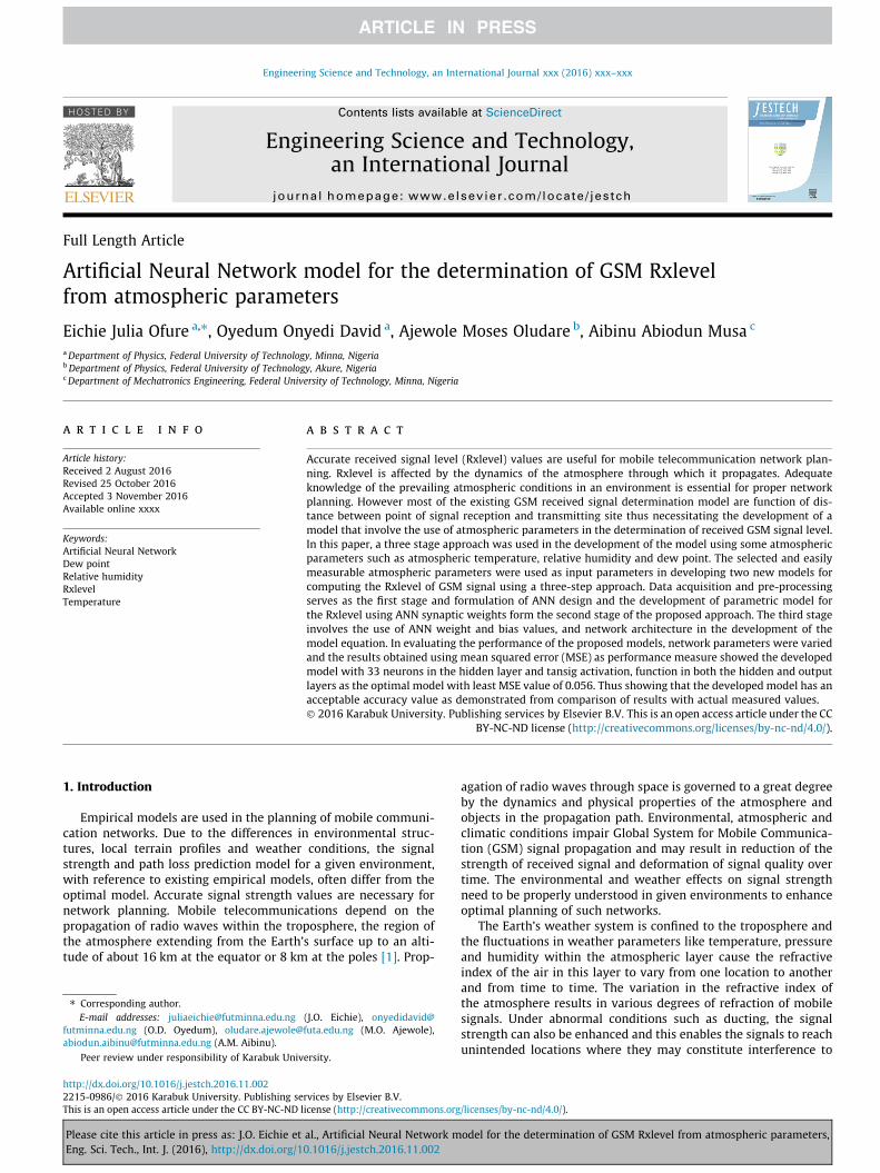
Table 1Best Performance in 20 Runs for 9 Pairs of Activation Function.

Hidden Layer Output Layer No. of Runs

Purelin Purelin 6Purelin Tansig 16Purelin Logsig 5Logsig Purelin 5Logsig Tansig 14Logsig Logsig 20Tansig Tansig 14Tansig Logsig 7Tansig Purelin 9

Table 2Worst Performance in 20 Runs for 9 Pairs of Activation Function.

Hidden Layer Output Layer No. of Runs

Purelin Purelin 38

Purelin Tansig 18Purelin Logsig 6

87

Logsig purelin 2Logsig Tansig 18

198

Logsig Logsig 110

Tansig Purelin 4Tansig Tansig 7

1217

Tansig Logsig 10138

The number of runs, number of neurons in the hidden layer and the MSE values of the


t, and the network’s output, y,) was computed. The computederrors were used by the network performance function to optimizethe network and the default network performance function forfeedforward networks is mean squared error, MSE (the mean ofthe sum of the squared errors) which is given by:

MSE ¼ 1=NXNi¼1

ðeiÞ2 !

ð21Þ

MSE ¼ 1=NXNi¼1

ðti � yiÞ2 !

ð22Þ

where N is the number of sets in the output data. The weight andbias values are adjusted so as to minimize the mean squared errorand thus increase the network performance. After the adjustments,the network undergoes a retraining process, the mean square erroris recomputed and the weight and bias values are readjusted. Theretraining continues until the training data achieves the desiredmapping to obtain minimum mean square error value.

4. Results and discussion

The performances of the developed ANN based Rxlevel modelswere evaluated using MSE. For each of the activation function pair,the best and worst performed networks in the 20 run of the scriptfile were determined with the least and highest MSE value. Tables1 and 2 show the performance comparison of the best and worstnetworks for each of the 9 pairs of activation function.

As can be seen from Tables 1 and 2, the number of run of thescript file has no obvious effect on the performance of the trained

No. of Neurons in hidden layer MSE

5 0.508415 0.511815 0.511831 0.127033 0.060233 0.061533 0.056633 0.065131 0.0995

No. of Neurons in hidden layer MSE

17 0.508411 0.508415 0.511819 2.532921 2.532927 2.53299 0.521111 2.532917 2.532921 2.532911 2.532915 2.53295 0.71659 2.532913 2.532917 2.53299 2.532919 2.532921 2.5329

worst performed networks are shown in bold font.



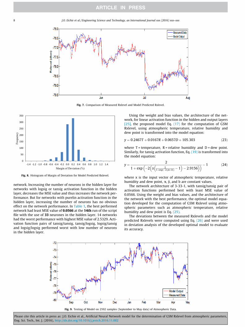
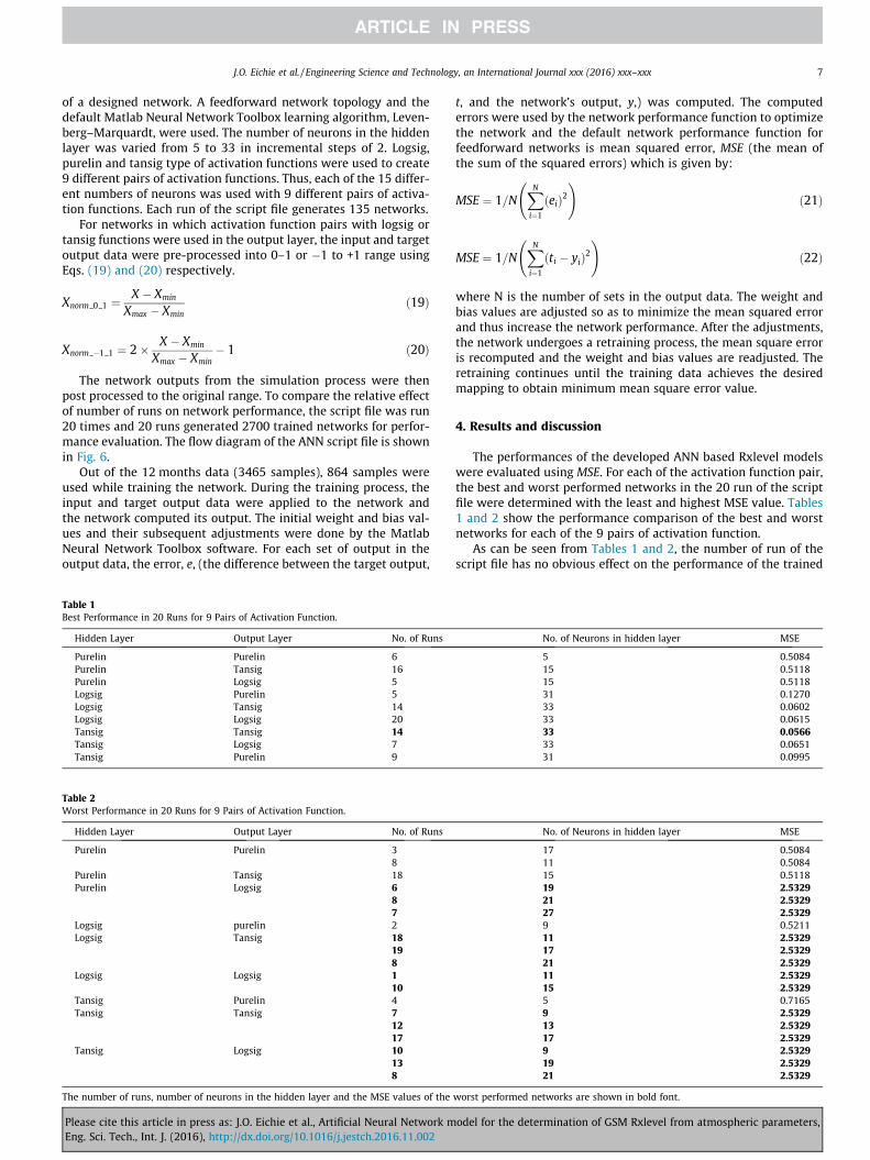
Fig. 7. Comparison of Measured Rxlevel and Model Predicted Rxlevel.

0

50

100

150

200

250

300

350

-1.4 -1.2 -1.0 -0.8 -0.6 -0.4 -0.2 0.0 0.2 0.4 0.6 0.8 1.0 1.2 1.4

Freq

uenc

y

Margin of Deviation (%)

Fig. 8. Histogram of Margin of Deviation for Model Predicted Rxlevel.


network. Increasing the number of neurons in the hidden layer fornetworks with logsig or tansig activation function in the hiddenlayer, decreases the MSE value and thus increases the network per-formance. But for networks with purelin activation function in thehidden layer, increasing the number of neurons has no obviouseffect on the network performance. In Table 1, the best performednetwork had least MSE value of 0.0566 at the 14th run of the scriptfile with the use of 33 neurones in the hidden layer. 14 networkshad the worst performance with highest MSE value of 2.5329. Acti-vation function pairs of tansig/tansig, tansig/logsig, logsig/tansigand logsig/logsig performed worst with low number of neuronsin the hidden layer.

Fig. 9. Testing of Model on 2592 samples (Sep


Using the weight and bias values, the architecture of the net-work, for linear activation function in the hidden and output layers[25], the proposed model Eq. (17) for the computation of GSMRxlevel, using atmospheric temperature, relative humidity anddew point is transformed into the model equation:

y ¼ 0:2467T þ 0:0167Rþ 0:0657Dþ 105:303 ð23Þ

where T = temperature, R = relative humidity and D = dew point.Similarly, for tansig activation function, Eq. (19) is transformed intothe model equation:

y ¼ 2

1þ exp �2 a 21þexpð�2ðbxþbÞÞ � 1� �

� 2:9156� �� 1 ð24Þ

where x is the input vector of atmospheric temperature, relativehumidity and dew point, a, b, and b are constant values.

The network architecture of 3-33-1, with tansig/tansig pair ofactivation functions performed best with least MSE value of0.0566. Using the weight and bias values, and the architecture ofthe network with the best performance, the optimal model equa-tion developed for the computation of GSM Rxlevel using atmo-spheric parameters such as atmospheric temperature, relativehumidity and dew point is Eq. (25).

The deviations between the measured Rxlevels and the modelpredicted Rxlevels were computed using Eq. (26) and were usedin deviation analysis of the developed optimal model to evaluateits accuracy.

tember to May data) of Atmospheric Data.



0

100

200

300

400

500

600

700

800

-2.0 -1.8 -1.6 -1.4 -1.2 -1.0 -0.8 -0.6 -0.4 -0.2 0.0 0.2 0.4 0.6 0.8 1.0 1.2 1.4 1.6 1.8 2.0

Freq

uenc

y

Margin of Deviation (%)

Fig. 10. Histogram of Margin of Deviation for Model Predicted Rxlevel when Tested on 2592 Samples.


Margin of deviation ¼ ym � yp

ym

� � 100 ð25Þ

where ym = measured Rxlevel and yp = model predicted Rxlevel. Themodel was used on 2592 samples (September to May data). Com-parison was made between the measured Rxlevels and the modelpredicted Rxlevels.

Fig. 7 shows plots of measured Rxlevels and model predictedRxlevels, and histogram of the margin of deviation for the modelpredicted Rxlevel is shown in Fig. 8.

The measured Rxlevel and model determined Rxlevel had corre-lation value of 0.706 when computed with Pearson correlationcoefficient formula:

r ¼ nðP xyÞ � ðP xÞðP yÞffiffiffiffiffiffiffiffiffiffiffiffiffiffiffiffiffiffiffiffiffiffiffiffiffiffiffiffiffiffiffiffiffiffiffiffiffiffiffiffiffiffiffiffiffiffiffiffiffiffiffiffiffiffiffiffiffiffiffiffiffiffiffiffiffiffiffiffiffiffiffiffiffi½nP x2 � ðP xÞ2�½nP y2 � ðP yÞ2�

q ð26Þ

wherer = Pearson correlation coefficientx = values in first set of datay = values in second set of datan = total number of values

Fig. 8 shows that the deviation distribution is concentratedaround 0 and this conotes acceptable accuracy of the model [17].Result obtained from the use of the model on 2592 samples(September to May data) is shown in Fig. 9 and the computed cor-relation coefficient value was 0.906. The histogram of margin ofdeviation shown in Fig. 10, shows that the developed model hasan acceptable accuracy.

5. Conclusion

In this study atmospheric temperature, relative humidity anddew point, were used as inputs in the development of ANN basedRxlevel determination parametric model for the determination ofreceived GSM signal level. Network parameters such as numberof neurons in the hidden layer and activation function were variedduring the performance evaluation process. The use of Levenberg-Marquard algorithm, network architecture of 3-33-1, tansig activa-tion function in both the hidden layer and output layer was theoptimal combination that gave the best performance with leastMSE value of 0.056. The weight and bias values and the architec-ture of the MLP network were used in the development of a modelequation. Comparisons of the measured and model output, showedthat the developed model can efficiently determine the GSM Rxle-vel using atmospheric temperature, relative humidity and dewpoint as input parameters.


Funding

This research did not receive any specific grant from fundingagencies in the public, commercial, or not-for-profit sectors.

Acknowledgment

The data used in this paper were obtained from the NECOPweather station in the Bosso campus of the Federal University ofTechnology, Minna, Nigeria and it was provided by the Centre forBasic Space Science, University of Nigeria, Nsukka. The authorsare grateful to the centre for providing the weather station.

References

[1] B.M. Reddy, Physics of the Troposphere, in: Handbook on Radio Propagation forTropical and Subtropical Countries, URSI committee on developing countries,UNESCO subvention, New Delhi, 1987, pp. 59–77.

[2] E.K. Smith, S. Weintraub, 1953, Proceedings of the Institute of Radio Engineers(IRE), 41, 1035

[3] B.R. Bean, B.A. Cohoon, Correlation of monthly median transmission loss andrefractive index profile characteristics, J. Res. Nat. Bur. Stand. 65D (1) (1961)67–74.

[4] M.P. Hall, Effects of the Troposphere on Radio Communications, PeterPeregrinus, 1979.

[5] I.E. Owolabi, V.A. Williams, Surface radio refractivity patterns in Nigeria andthe Southern Cameroon, J. West Afr. Sci. Assoc. 15 (1970) 3–17.

[6] O.D. Oyedum, G.K. Gambo, Surface radio refractivity in Northern Nigeria, Niger.J. Phys. 6 (1994) 36–41.

[7] A.U. Usman, O.U. Okereke, E.E. Omizegba, Instantaneous GSM signal strengthvariation with weather and environmental factors, Am. J. Eng. Res. (AJSER) 4(3) (2015) 104–115.

[8] A.S. Adewumi, M.O. Alade, H.K. Adewumi, Influence of air temperature, relativehumidity and atmospheric moisture on UHF radio propagation in SouthWestern Nigeria, Int. J. Sci. Res. (IJSR) 4 (8) (2015) 588–592.

[9] J. Luomala, I. Hakala, Effects of temperature and humidity on radio signalstrength in outdoor wireless sensor networks, Proc. Federated Conf. Comput.Sci. Inf. Syst. 5 (2015) 1247–1255.

[10] M. Zilinskas, M. Tamosiunaite, S. Tamosiunas, M. Tamosiuniene, E.Stankevicius, 2015, The infuence of atmospheric radio refractivity on theWiMAX signal level in the areas of weak coverage, progress In:Electromagnetics Research Symposium Proceedings, Prague, Czech Republic,pp. 580–584.

[11] M. Afrand, A.A. Nadooshan, M. Hassani, H. Yarmand, M. Dahari, Predicting theviscosity of multi-walled carbon nanotubes/water nanofluid by developing anoptimal artificial neural network based on experimental data, Int. Commun.Heat Mass 77 (2016) 49–53.

[12] H. Elçiçek, E. Akdogan, S. Karagöz, The use of artificial neural network forprediction of dissolution kinetics, Sci. World J. 2014 (2014) 1–9.

[13] D. Deligiorgi, K. Philippopoulos, G. Kouroupetroglou, Artificial neural networkbased methodologies for the spatial and temporal estimation of airtemperature, Int. Conf. Pattern Recognit. Appl. Methods (2013) 669–678.

[14] J.O. Famorji, M.O. Oyeleye, A test of the relationship between refractivity andradio signal propagation for dry particulates, Res. Desk 2 (4) (2013) 334–338.

[15] O. Sheowu, L.A. Akinyemi, Effect of climatic change on GSM signal, Res. J.Comput. Syst. Eng. – RJCSE 4 (2) (2013) 471–478.

[16] M. Afrand, D. Toghraie, N. Sina, Experimental study on thermal conductivity ofwater-based Fe3O4 nanofluid: development of a new correlation and modeledby artificial neural network, Int. Commun. Heat Mass 75 (2016) 262–269.


http://refhub.elsevier.com/S2215-0986(16)30689-9/h0105











































[17] M. Afrand, K.N. Najafabadi, N. Sina, M.R. Safaei, A.S. Kherbeet, S. Wongwises, M.Dahari, Prediction of dynamic viscosity of a hybrid nano-lubricant by anoptimal artificial neural network, Int. Commun. Heat Mass Transfer 76 (2016)209–214.

[18] K. Philippopoulos, D. Deligiorgi, Application of artificial neural networks forthe spatial estimation of wind speed in a coastal region with complextopography, Renew. Energ. 38 (2012) 75–82.

[19] M.H. Esfe, M. Afrand, S. Wongwises, A. Naderi, A. Asadi, S. Rostami, M. Akbari,Application of feedforward multilayer perceptron artificial neural networksand empirical correlation for prediction of thermal conductivity of Mg(OH)2–EG using experimental data, Int. Commun. Heat Mass Transfer 67 (2015)(2015) 46–50.

[20] A.J. Litta, S.M. Idicula, U.C. Mohanty, Artificial neural network model inprediction of meteorological parameters during premonsoon thunderstorms,Int. J. Atmos. Sci. (2013) 1–14.


[21] S. Ballı, I. Tarımer, An application of artificial neural networks for predictionand comparison with statistical methods, Elektronika ir Elektrotechnika(Electron. Electr. Eng.) 10 (2) (2013) 101–105.

[22] Y.H. Hu, J.-N. Hwang, Handbook of Neural Network Signal Processing, CRCPress, Boca Raton, 2002.

[23] M.H. Beale, M.T. Hagan, B.D. Howard, 2011. Neural Network ToolboxTM 7. UserGuide, R2011b.

[24] A.M. Aibinu, A.A. Shafie, M.J.E. Salami, Performance analysis of ANN basedYCbCr skin detection algorithm, Procedia Eng. 41 (2012) 1183–1189.

[25] A.M. Aibinu, M.J.E. Salami, A.A. Shafie, Artificial neural network basedautoregressive modeling techniques with application in voice activitydetection, Eng. Appl. Artif. Intell. 25 (2012) 1255–1275.
































artificial neural network model for the determination of gsm … · full length article artiﬁcial...

Documents