arxiv:funct-an/9703001v3 6 feb 1998funct-an/9703001v3 6 feb 1998 preprint funct-an/9703001, 1997 two...

arX

iv:f

unct

-an/

9703

001v

3 6

Feb

199

8

Preprint funct-an/9703001,1997

Two Approaches to

Non-Commutative Geometry∗

Vladimir V. KisilInstitute of Mathematics

Economics and MechanicsOdessa State University

ul. Petra Velikogo, 2Odessa-57, 270057, UKRAINE

E-mail: [email protected]

April 1, 1997; Revised February 3, 1998

Abstract

Looking to the history of mathematics one could find out two outerapproaches to Geometry. First one (algebraic) is due to Descartes

and second one (group-theoretic)—to Klein. We will see that theyare not rivalling but are tied (by Galois). We also examine theirmodern life as philosophies of non-commutative geometry. Connec-tions between different objects (see keywords) are discussed.

∗Supported by grant 3GP03196 of the FWO-Vlaanderen (Fund of Scientific Research-Flanders), Scientific Research Network “Fundamental Methods and Technique in Mathe-matics”.

1991 Mathematical Subject Classification. Primary: 46H30; Secondary: 30G35,47A13, 81R05.

Keywords and phrases. Heisenberg group, Weyl commutation relation, Maninplane, quantum groups, SL(2,R), Hardy space, Bergman space, Segal-Bargmann space,Szego projection, Bergman projection, Clifford analysis, Cauchy-Riemann-Dirac opera-tor, Mobius transformations, functional calculus, Weyl calculus (quantization), Berezinquantization, Wick ordering, quantum mechanics.

1

http://arxiv.org/abs/funct-an/9703001v3

2 Vladimir V. Kisil

Contents

1 Introduction 2

2 Coordinates: from Descartes to Nowadays 3

3 Klein, Galois, Descartes 5

4 The Heisenberg Group and Symmetries of the Manin Plain 7

5 Analytic Function Theory from Group Representations 9

5.1 Wavelet Transform and Coherent States . . . . . . . . . . . . . . . 10

5.2 Reduced Wavelets Transform . . . . . . . . . . . . . . . . . . . . . 12

5.3 Great Names . . . . . . . . . . . . . . . . . . . . . . . . . . . . . . 15

6 The Name of the Game 17

7 Non-Commutative Conformal Geometry 23

8 Do We Need That Observables Form an Algebra? 26

9 Conclusion 30

10 Acknowledgments 31

1 IntroductionDescartes was the first great modern philosopher, afounder of modern biology, a first-rate physicist, andonly incidentally a mathematician.

M. Kline [29, § 15.3].

If one takes a look on mathematics as a collection of facts about a largediversity of objects covered by the Mathematic Subject Classification bydigits from 00 till 93, then it will be difficult to explain why we are referring tomathematics as a “united and inseparable” science. Even the common originof all mathematical fields laid somewhere in Elements of Euclid hardlybe an excuse. Indeed western philosophy and psychology as well commonlyrooted in works of Great Greeks (Plato or Aristotle?), but it will beoffensive for a philosopher as well as for a psychologist do not distinguishthem nowadays. In contrast, in mathematics the most exiting and welcomeresults usually combine facts, notions and ideas of very remote fields (thealready classical example is Atiah-Singer theorem linking algebra, analysisand geometry).

Two Approaches to Non-Commutative Geometry 3

So even while exponentially growing mathematical facts remain linkedby some underlying ideas, which are essentially vital for the mathematicalenterprise. Thus it seems worth enough for a mathematician to think (andsometime to write) not only about new mathematical facts but also aboutold original ideas. Particularly relations between new facts and old ideasdeserve special attention.

In this paper we return to two great ideas familiar to every mathe-matician: Coordinate method of R. Descartes and Erlangen program ofF. Klein. They specify two different approaches to geometry and becomeactual now in connections with such an interesting and fascinate area ofresearch as non-commutative geometry [12, 36].

The paper format is as follows. After some preliminary remarks in Sec-tions 2–4 we will arrive to paper’s core in Section 5: it is an abstract scheme ofanalytic function theories. We will interpret classic examples accordingly tothe presented scheme in Section 6. In Section 7 we will expand considerationto non-commutative spaces with physical application presented in Section 8.For a reader primary interested in analytic function theory Section 5 and 6form an independent reading.

A feature of the paper is a healthy portion of self-irony. It will not be anabuse if a reader will smile during the reading as the author did during thewriting.

2 Coordinates: from Descartes to Nowadays

. . . coordinate geometry changed the face of mathe-matics.

M. Kline [29, § 15.6].

The first danger of a deep split in mathematics condensed before 17-thcentury. The split shown up between synthetic geometry of Greeks and ab-stract algebra of Arabs. It was overcome by works of Fermat andDescartes

on analytic geometry. Descartes pointed out that geometric construction callfor adding, subtracting, multiplying, and dividing segments of lines. But thisis exactly four operations of algebra. So one could express and solve geomet-ric problems in algebraic terms. The crucial steps are:

1. To introduce a coordinate system, which allows us to label geometricalpoints by sets of numbers or coordinates. Of course, coordinates arefunctions of points.

2. To link desired geometrical properties and problems with equations ofcoordinate. Then solutions to equations will give solutions of originalgeometric problems.

4 Vladimir V. Kisil

Four algebraic operations suggest to consider coordinates from Step 1 asmembers of a commutative algebra of functions of geometric points. More-over, it seems unavoidable to use other functions from this algebra to con-struct and solve equations from Step 2. In such a way the commutativealgebra of functions become the central object of new analytic geometry.From geometry this algebra inherits some additional structures (metrical,topological, etc.)

Having a vocabulary that allows us to translate from the geometricallanguage to algebraic one nothing could prevent one to use it in the oppo-site direction: what are geometrical counterparts of such and such algebraic

notions? Particularly, what will happen if we start from an arbitrary commu-tative algebra (with a relevant additional structure) instead coordinate one?The answer to a question of this type is given by the celebrated theorem ofI.M. Gelfand and M.A. Naimark [24, § 4.3]:

Theorem 2.1 (Gelfand-Naimark) Any commutative Banach algebra A

could be realized as the algebra C(X) of all continuous functions over atopological space X . The points of X are labelled by the maximal ideals (orcharacters) of A.

So looking for adventures and new experience in geometry one should tryto begin from non-commutative algebras. This gives the name of resultingtheory as non-commutative geometry. Very attractive (and in some sensearchetypical) object is anticommutative coordinates, which satisfy to identityx1x2 = −x2x1 instead of commutation rule x1x2 = x2x1:

In recent years, several attempts have been made to developanticommutative analogs of geometric notions. Most of theseattempts are rooted in one of the great ideas of mathematics inthis century, the idea that geometry is recovered from algebra bytaking prime or maximal ideals of a commutative ring. Thus onereplaces a commutative ring by an exterior algebra and one triesto do something similar. [8]

On this road one could found natural unification of vector geometry andGrassmann algebras.

There are still many other opportunities. As it always happens with gen-eralizations of a non-trivial notion, there is no the non-commutative geometrybut there are non-commutative geometries (for example, [12] and [36]).

Remark 2.2 It is important that all described constructions deserve thename of geometry not only by peculiar rules of the game named mathematics


Commutative - Classic Non-Commutative - QuantumComplex variables Operator in Hilbert spaceReal variables Selfadjoint operators

Infinitesimal variable Compact operatorInfinitesimal of order α µn(T ) = O(n−α)

Integral∫T = log trace T

Table 1: Vocabulary between Commutative-Classic and Non-Commutative-Quantum Geometries. Here µn(T ) is stand for n-th eigenvalue of a compactoperator T .

but also by their relations with the real word. Their ambitions are to describethe structure of actual space(-time) on the quantum level (see Section 8) ex-actly as classic geometry succeed it for the Nile valley. Thus as commutativegeometry is the language of classic mechanics so non-commutative geometryis supposed to be a language for quantum physics. So in modern sciencenon-commutative and quantum are usually synonymous.

Example 2.3 Quantummechanics begun from the Heisenberg commutationrelations XY = Y X + i~I and was a source of inspiration for functionalanalysis. Thus an additional structure on non-commutative algebra, whichdescribes geometrical objects, comes often from operator theory. Table 1contains a vocabulary for non-commutative geometry taken from [7], whichis devoted to description of quantized theory of gravitational field.On this way one could find such exiting examples as a curvature or a

connection on a geometric set consisting of two points only [12]. We willdiscuss such a vocabulary with more details in Section 8.

3 Klein, Galois, Descartes

. . . not all of geometry can be incorporated in Klein’sscheme.

M. Kline [29, § 38.5].

The second (group-theoretic) viewpoint on geometry was expressed byF. Klein in his famous Erlangen program and seems unrelated to coordinategeometry. But this is not true.

Theorem 3.1 The difference between Klein and Descartes is Galois or

Klein(1872) = Galois(1831) +Descartes(1637) (3.1)

6 Vladimir V. Kisil

Proof. The idea of Descartes to reduce geometric problems to the algebraicequations was a brilliant prophecy regarding to the very modest knowledgeabout algebraic equations in that times. Although his contemporaries couldsolve already algebraic equations up to fourth degree, i.e., the most generalthat could be solved in radicals, the general theory of algebraic equation wasnot even supposed to exist. It is enough to say that for Descartes1 evennegative roots of an equation were false roots not speaking about complexones [29, §13.5].

We were lucky that another genius, namely Galois, leaves to us a mes-sage at the end of his very short life: solvability of equations could be de-

termined via its group of symmetries. Again we could skip all facts of cor-responding theory (for elementary account see for example [29, § 31.4]) andjust add it to the coordinate geometry2. The result will almost identical withthe Erlangen program [29, § 38.5]:

Definition 3.2 Every geometry can be characterized by a group (of trans-formations) and that geometry is really concerned with invariants under thisgroup.

To see this achievement in the proper light one should keep in mind thatthe notion of abstract group was fully recognized only years after Erlangenprogram [29, § 49.2] (as the notion of a root to an equation was recognizedyears after Descartes’ coordinate geometry).

Corollary 3.3 Klein is greater than Descartes:

Klein > Descartes

Proof. Galois is obviously positive (Galois > 0), so the (3.1) implies theassertion.

Problem 3.4 Find a counterexample to the last Corollary.

Hint. See the epigraph.Even not being universal the Erlangen program offers a way to classify

the variety of geometries by means of associated groups [29, § 38.5]. We willlink in the Erlangen spirit different analytic function theories and connectedfunctional calculi with group representations. This gives an opportunity tomake their classification too.

1We could be surprised how little a genius should be acquainted with mathematicalfacts to discover the underlying fundamental idea.

2Note the appearance of a geometric problem in [29, § 31.5] immediately after theGalois theory in [29, § 31.4]


Remark 3.5 The connection jokingly presented in this section is often un-observed but is very important. In concrete situations it takes practicalforms. Many connections between non-commutative geometry and grouprepresentations are mentioned in [42]. For example, an early result on non-commutative geometry—the classification of von Neumann factors of typeIII—was carried out by means their group of automorphisms [12] (see alsoRemarks 6.4 and 7.2). And that is also important, such a connection gen-erates a hope that not only particular mathematical facts are linked by fun-damental ideas, but also these ideas are connected one with another on adeeper level.

4 The Heisenberg Group and Symmetries of

the Manin Plain. . . I want to popularize the Heisenberg group, whichis remarkably little known considering its ubiquity.

R. Howe [19].

What does Erlangen program tell to a non-commutative geometer? Onecould do non-commutative geometry considering (quantum) symmetries ofnon-commutative (=quantum) objects. This approach leads to quantumgroups [22, 35, 36]. We will consider a simple example of Mq(2).

We have mentioned already (see Remark 2.3) the Heisenberg commuta-tion relation:

[X, Y ] = I. (4.1)

Here X , Y , and I, viewed as generators of a Lie algebra, produce a Liegroup, which is the celebrated Heisenberg (or Weyl) group H1 [17, 19, 44].An element g ∈ Hn (for any positive integer n) could be represented asg = (t, z) with t ∈ R, z = (z1, . . . , zn) ∈ Cn and the group law is given by

g ∗ g′ = (t, z) ∗ (t′, z′) = (t+ t′ +1

2

n∑

j=1

ℑ(zjz′j), z + z′), (4.2)

where ℑz denotes the imaginary part of a complex number z. Of course theHeisenberg group is non-commutative and particularly one could find out forH1:

(0, 1) ∗ (0, i) = (1, 0) ∗ (0, i) ∗ (0, 1) (4.3)

The last formula is usually called the Weyl commutation relation and is theintegrated (or exponentiated) form of (4.1).

Now let us consider a continuous irreducible representation [24, 44] π :H1 → A of the Heisenberg group in a C∗-algebra A. Then elements of the

8 Vladimir V. Kisil

center of H1, which are of the form (t, 0), will map to multipliers ae of theidentity e ∈ A. For unitary representations we have |a| = 1 for all such a.

Let x = π(0, 1), y = π(0, i), qe = π(1, 0). Then the Weyl commutationrelation (4.3) will correspond to

xy = qyx (4.4)

The last equation is taken by Yu. Manin [35] as the defining relation forquantum plane, which is also often called the Manin plane. As we saw theManin plane is a representation of the Heisenberg-Weyl group and thus couldbe named3 Heisenberg-Weyl-Manin plane. More formal: Manin plane with aparameter q ∈ C is the quotient of free algebra generated by elements x andy subject to two-sided ideal generated by the quadratic relation (4.4).

Let us consider the regular representation πr of H1 as right shifts onL

2(H1) and let M be an algebra of operators generated by xr = πr(0, 1) and

yr = πr(0, i). Then Manin plane is a representation π of M under whichx = π(xr) and y = π(yr). Moreover an algebraic identity f(x, y) = 0 holds

on Manin plane for all q ∈ C if and only if the algebraic identity f(xr, yr) = 0is true in M.

Connection between the Manin plane and the Weyl commutation rela-tion was already mentioned in [35] but was not used explicitly. Thus thisconnection disappeared from the following works. Even fundamental trea-tise [22] (which has 531 pages!) mentioned the Heisenberg group only twiceand in both cases disconnected with the Manin plane. This is especially pitybecause the Heisenberg group could give new incites for quantum groups, asit does for the Manin plane.

Example 4.1 4 As it was mentioned at the beginning of the section thequantum group could be viewed as symmetries of quantum object. Partic-

ularly Mq(2) is a set of 2 × 2 matrixes

(a bc d

), “which maps the Manin

plane to the Manin plane”, namely if x and y satisfy to (4.4) and(a bc d

)(xy

)=

(ax+ bycx+ dy

)

then x′ = ax + by, y′ = cx + dy should again satisfy to (4.4). From this

condition for both matrixes

(a bc d

)and

(a cb d

)one could find that

3Now and then the nobility of a mathematical object is measured by the number of itsfamily names.

4For brevity the Example is presented very informal. We believe that this is not anabuse.


entries a, b, c, and d of

(a bc d

)are subject to the following six identities:

ab = q−1ba, ac = q−1ca, db = qbd, dc = qcd (4.5)

bc = cb, [a, d] = −(q − q−1)cb (4.6)

To keep anytime in mind all six identities for any element of Mq(2) is a littlebit laborious, isn’t it? The Heisenberg group proposes an elegant way out. 2-

vector

(xy

)on the Manin plane is of course an element of a representation

of H2 as the Manin plane itself is a representation of H1. And it is easyto check that due to celebrated Stone-von Neumann theorem [17, 44] sixidentities (4.5)–(4.6) up to unitary equivalence prescribe that a, b, c, d belongto a representation πM of H2 such that:

a = πM(0, 1, 1), b = πM(0, 1, i), c = πM(0, i, 1), d = πM (0, i, i).

Then a product of two elements ofMq(2) is naturally described via represen-tation of H4 (because entries of different elements pairwise commutes) andso far. Thus Mq(2) is a representation of M2(πM(H∞)). There is no problemto think over H∞ because consideration is purely algebraic and no topologyis involved. Alternatively one could consider HN for some unspecified suffi-ciently large N . Of course, our conclusion about algebraic identities on theManin plane remains true for Mq(2).

5 Analytic Function Theory from Group Rep-

resentationsI learned from I.M. Gel’fand that Mathematics of anykind is a representation theory. . .

Yu. I. Manin,Short address on occasion of Professor Gel’fand 70thbirthday.

One could notice that through glasses of Erlangen program the boundarybetween commutative and non-commutative geometry becomes tiny. Quan-tum groups became a representation of classic group and the word non-

commutative is not distinguishing any more. Indeed, the group of symmetriesof Euclidean geometry is non-commutative (think on a composition of a shiftand a rotation) and a group could act as symmetries of classic and quantumobject (symplectic transformations). And even more: the difference betweengeometry and, say, analysis became unnoticeable.

In this section we are going to proof the following5

5We are continuing the definition-theorem-proof style presentation of Section 3.

10 Vladimir V. Kisil

Theorem 5.1 Complex analysis = conformal geometry.

Proof. The group of conformal mapping (particularly for the unit disk theyare fraction-linear transformations) plays an important role in any textbookon complex analysis [33, Chap. 10], [38, Chap. 2]. Moreover, two key object ofcomplex analysis, namely the Cauchy-Riemann equations and Cauchy kernel,are invariants with respect to these transformations. Thus the Theoremfollows from Definition 3.2.

5.1 Wavelet Transform and Coherent States

We agree with a reader if he/she is not satisfied by the last short proof andwould like to see a more detailed account how the core of complex analysiscould be reconstructed from representation theory of SL(2,R). We presentan abstract scheme, which also could be applied to other analytic functiontheories [10, 27]. We start from a dry construction followed in the nextSection by classic examples, which will justify our usage of personal names.

Let X be a topological space and let G be a group that acts G : X → Xas a transformation g : x 7→ g · x from the left, i.e., g1 · (g2 · x) = (g1g2) · x.Moreover, let G act on X transitively. Let there exist a measure dx on Xsuch that a representation π(g) : f(x) 7→ m(g, x)f(g−1 · x) (with a functionm(g, h)) is unitary with respect to the scalar product 〈f1(x), f2(x)〉L2(X) =∫Xf1(x)f2(x) d(x), i.e.,

〈[π(g)f1](x), [π(g)f2](x)〉L2(X) = 〈f1(x), f2(x)〉L2(X) ∀f1, f2 ∈ L2(X).

We consider the Hilbert space L2(X) where representation π(g) acts by uni-tary operators.

Remark 5.2 It is well known that the most developed part of representationtheory consider unitary representations in Hilbert spaces. By this reasonwe restrict our attention to Hilbert spaces of analytic functions, the areausually done by means of the functional analysis technique. We also assumethat our functions are complex valued and this is sufficient for examplesexplicitly considered in the present paper. However the presented scheme isworking also for vector valued functions and this is the natural environmentfor Clifford analysis [6], for example. One also could start from an abstractHilbert space H with no explicit realization as L2(X) given.

LetH be a closed compact6 subgroup ofG and let f0(x) be such a function6While the compactness will be explicitly used during our abstract consideration, it is

not crucial in fact. Example 6.3 will show how one could make a trick for non-compactH .


that H acts on it as the multiplication

[π(h)f0](x) = χ(h)f0(x) , ∀h ∈ H, (5.1)

by a function χ(h), which is a character of H i.e., f0(0) is a common eigen-function for all operators π(h). Equivalently f0(x) is a common eigenfunctionfor operators corresponding under π to a basis of the Lie algebra of H . Notealso that |χ(h)|2 = 1 because π is unitary. f0(x) is called vacuum vector

(with respect to subgroup H). We introduce the F2(X) to be the closed linersubspace of L2(X) uniquely defined by the conditions:

1. f0 ∈ F2(X);

2. F2(X) is G-invariant;

3. F2(X) is G-irreducible.

Thus restriction of π on F2(X) is an irreducible unitary representation.The wavelet transform7 W could be defined for square-integral represen-

tations π by the formula [25]

W : F2(X) → L∞(G)

: f(x) 7→ f(g) = 〈f(x), π(g)f0(x)〉L2(X) (5.2)

The principal advantage of the wavelet transform W is that it express therepresentation π in geometrical terms. Namely it intertwins π and left regularrepresentation λ on G:

[λgWf ](g′) = [Wf ](g−1g′) = 〈f, πg−1g′f0〉 = 〈πgf, πg′f0〉 = [Wπgf ](g′),(5.3)

i.e., λW = Wπ. Another important feature of W is that it does not lose in-formation, namely function f(x) could be recovered as the linear combination

of coherent states fg(x) = [πgf0](x) from its wavelet transform f(g) [25]:

f(x) =

∫

G

f(g)fg(x) dg =

∫

G

f(g)[πgf0](x) dg, (5.4)

where dg is the Haar measure on G normalized such that∫G

∣∣∣f0(g)∣∣∣2

dg = 1.

One also has an orthogonal projection P from L2(G, dg) to image F2(G, dg)

7The subject of coherent states or wavelets have been arising many times in manyapplied areas and the author is not able to give a comprehensive history and propercredits. One could mention important books [13, 28, 37]. We give our references by recentpaper [25], where applications to pure mathematics were considered.


of F2(X) under wavelet transform W, which is just a convolution on g with

the image f0(g) = W(f0(x)) of the vacuum vector [25]:

[Pw](g′) =∫

G

w(g)f0(g−1g′) dg. (5.5)

5.2 Reduced Wavelets Transform

Our main observation will be that one could be much more economical (ifsubgroup H is non-trivial) with a help of (5.1): in this case one need to know

f(g) not on the whole group G but only on the homogeneous space G/H [1,§ 3].

Let Ω = G/H and s : Ω → G be a continuous mapping [24, § 13.1].Then any g ∈ G has a unique decomposition of the form g = s(a)h, a ∈ Ωand we will write a = s−1(g), h = r(g) = (s−1(g))

−1g. Note that Ω is a

left G-homogeneous space8 with an action defined in terms of s as follow:g : a 7→ s−1(g · s(a)). Due to (5.1) one could rewrite (5.2) as:

f(g) = 〈f(x), π(g)f0(x)〉L2(X)

= 〈f(x), π(s(a)h)f0(x)〉L2(X)

= 〈f(x), π(s(a))π(h)f0(x)〉L2(X)

= 〈f(x), π(s(a))χ(h)f0(x)〉L2(X)

= χ(h)〈f(x), π(s(a))f0(x)〉L2(X)

Thus f(g) = χ(h)f(a) where

f(a) = [Cf ](a) = 〈f(x), π(s(a))f0(x)〉L2(X) (5.6)

and function f(g) on G is completely defined by function f(a) on Ω. For-mula (5.6) gives us an embedding C : F2(X) → L∞(Ω), which we will callreduced wavelet transform. We denote by F2(Ω) the image of C equippedwith Hilbert space inner product induced by C from F2(X).

Note a special property of f0(g) and f0(a):

f0(h−1g) = 〈f0, πh−1gf0〉 = 〈πhf0, πgf0〉 = 〈χ(h)f0, πgf0〉 = χ(h)f0(g).

It follows from (5.3) that C intertwines ρC = Cπ representation π with therepresentation

[ρgf ](a) = f(s−1(g · s(a)))χ(r(g · s(a))). (5.7)8Ω with binary operation (a1, a2) 7→ s−1(s(a1) · s(a2)) becomes a loop of the most

general form [39]. Thus theory of reduced wavelet transform developed in this subsectioncould be considered as wavelet transform associated with loops. However we prefer todevelop our theory based on groups rather on loops.


While ρ is not completely geometrical as λ in applications it is still moregeometrical than original π. In many cases ρ is representat induced by thecharacter χ.

If f0(x) is a vacuum state with respect to H then fg(x) = χ(h)fs(a)(x)and we could rewrite (5.4) as follows:

f(x) =

∫

G

f(g)fg(x) dg

=

∫

Ω

∫

H

f(s(a)h)fs(a)h(x) dh da

=

∫

Ω

∫

H

f(a)χ(h)χ(h)fs(a)(x) dh da

=

∫

Ω

f(a)fs(a)(x) da ·∫

H

|χ(h)|2 dh

=

∫

Ω

f(a)fs(a)(x) da,

if the Haar measure dh on H is set in such a way that∫H|χ(h)|2 dh = 1 and

dg = dh da. We define an integral transformation F according to the lastformula:

[F f ](x) =∫

Ω

f(a)fs(a)(x) da, (5.8)

which has the property FC = I on F2(X) with C defined in (5.6). One couldconsider the integral transformation

[Pf ](x) = [FCf ](x) =∫

Ω

〈f(y), fs(a)(y)〉L2(X)fs(a)(x) da (5.9)

as defined on whole L2(X) (not only F2(X)). It is known that P is an

orthogonal projection L2(X) → F2(X) [25]. If we formally use linearity ofthe scalar product 〈·, ·〉L2(X) (i.e., assume that the Fubini theorem holds) wecould obtain from (5.9)

[Pf ](x) =

∫

Ω

〈f(y), fs(a)(y)〉L2(X)fs(a)(x) da

= 〈f(y),∫

Ω

fs(a)(y)fs(a)(x) da〉L2(X)

=

∫

X

f(y)K(y, x) dµ(y), (5.10)

where

K(y, x) =

∫

Ω

fs(a)(y)fs(a)(x) da


With the “probability 12” (see discussion on the Bergman and the Szego ker-

nels bellow) the integral (5.10) exists in the standard sense, otherwise it is asingular integral operator (i.e, K(y, x) is a regular function or a distribution).

Sometimes a reduced form P : L2(Ω) → F2(Ω) of the projection P (5.5)is of a separate interest. It is an easy calculation that

[Pf ](a′) =∫

Ω

f(a)f0(s−1(a−1 · a′))χ(r(a−1 · a′)) da, (5.11)

where a−1 · a′ is an informal abbreviation for (s(a))−1 · s(a′). As we will seeits explicit form could be easily calculated in practical cases.

And only at the very end of our consideration we introduce the Taylorseries and the Cauchy-Riemann equations. One knows that they are startingpoints in the Weierstrass and the Cauchy approaches to complex analysiscorrespondingly.

For any decomposition fa(x) =∑

α ψα(x)Vα(a) of the coherent statesfa(x) by means of functions Vα(a) (where the sum could become eventuallyan integral) we have the Taylor series expansion

f(a) =

∫

X

f(x)fa(x) dx =

∫

X

f(x)∑

α

ψα(x)Vα(a) dx

=∑

α

∫

X

f(x)ψα(x) dxVα(a)

=

∞∑

α

Vα(a)fα, (5.12)

where fα =∫Xf(x)ψα(x) dx. However to be useful within the presented

scheme such a decomposition should be connected with structures of G andH . For example, if G is a semisimple Lie group and H its maximal compactsubgroup then indices α run through the set of irreducible unitary represen-tations of H , which enter to the representation π of G.

The Cauchy-Riemann equations need more discussion. One could observefrom (5.3) that the image of W is invariant under action of the left but rightregular representations. Thus F2(Ω) is invariant under representation (5.7),which is a pullback of the left regular representation on G, but its right coun-terpart. Thus generally there is no way to define an action of left-invariantvector fields on Ω, which are infinitesimal generators of right translations, onL2(Ω). But there is an exception. Let Xj be a maximal set of left-invariantvector fields on G such that

Xj f0(g) = 0.


Because Xj are left invariant we have Xj f′g(g) = 0 for all g′ and thus image

of W, which the linear span of f ′g(g), belongs to intersection of kernels of Xj.

The same remains true if we consider pullback Xj of Xj to Ω. Note that the

number of linearly independent Xj is generally less than for Xj. We call Xj

as Cauchy-Riemann-Dirac operators in connection with their property

Xj f(g) = 0 ∀f(g) ∈ F2(Ω). (5.13)

Explicit constructions of the Dirac type operator for a discrete series repre-sentation could be found in [3, 30].

We do not use Cauchy-Riemann-Dirac operator in our construction, butthis does not mean that it is useless. One could found at least such its niceproperties:

1. Being a left-invariant operator it naturally encodes an informationabout symmetry group G.

2. It effectively separates irreducible components of the representation πof G in L2(X).

3. It has a local nature in a neighborhood of a point vs. transformations,which act globally on the domain.

5.3 Great Names

It is the time to give names of Greats to our formulas. A surprising thing is:all formulas have two names, each one for different circumstances (judgmentswill be given in Section 6). More precisely we have two alternatives

1. X and Ω are not isomorphic as topological spaces with measures. ThenF2(X) becomes the Hardy space. The space L2(Ω) is Segal-Bargmann

space. We could consider (5.6) as an abstract analog of the Cauchy

integral formula, which recovers analytic function f(a) on Ω from its(boundary) values f(x) on X . The formula (5.8) could be named asBargamann inverse formula9. The orthogonal projection P (5.9) is theSzego projection and expression (5.10) is a singular integral operator. Inthis case of Hardy spaces we could not define a Hilbert space structureon F2(Ω) by means of a measure on Ω. Therefor we need to keep both

9The name is taken from the context of classical Segal-Bargmann space [4, 40] andstand for the mapping from the Segal-Bargmann space to L2(R

n). I do not know its namein the context of Hardy space, but it definitely should exist (it is impossible to find outsomething new for analytic functions in our times).


Notion Name for case X 6∼ Ω Name for case X ∼ Ω

Space F2(X) Hardy spaceBergman spaceSpace F2(Ω) Segal-Bargmann space

Formula (5.6) Cauchy IntegralBergman integralFormula (5.8) Segal-Bargmann inverse

Projection (5.10) Szego projectionBergman projectionProjection (5.11) Segal-Bargmann projection

Series (5.12) Taylor seriesOperator (5.13) Cauchy-Riemann-Dirac operator

Table 2: Abstract formulas and their classical names. The apparent period-icity of names is not a coincidence or author’s arbitrariness.

faces of our theory: the scalar product could be defined by a measureonly for F2(X) and analytic structure is defined via geometry of F2(Ω).

2. X and Ω are isomorphic as topological spaces with measures. In sharpcontrast to the previous case where no name appears twice, this casefully covered by single person, namely Bergman. On the other hand,because X ∼ Ω we have twice as less objects in this case. ParticularlyF2(X) ∼ F2(Ω) is known as the Bergman space. In this case repre-sentation π on F2(X) ∼ F2(Ω) due to embedding s : Ω → G couldbe treated as a part of left regular representation on L2(G) by shiftsand thus representation π belongs to discrete series [34, § VI.5]. Theorthogonal projection P (5.9) is the Bergman projection and expres-sion (5.10) is a regular integral operator.

Remark 5.3 The presented constructions being developed independentlyhas many common points with the theory of harmonic functions on sym-metric spaces (see for example [32]). The new feature presented here is theassociation of function theories with sets of data (G, π,H, f0) rather sym-metric spaces. This allows

1. To distinguish under the common framework the Hardy and differentBergman spaces, which are defined on the same symmetric space.

2. To deal with non-geometrical group action like in the case of the Segal-Bargmann space (see Example 6.3).

3. To apply it not only to semisimple but also nilpotent Lie groups (seeExample 6.3).


On the other hand Bargmann himself realizes that spaces of analytic func-tions give realizations of representations for semisimple groups and later thisidea was used many times (see for example [3], [18, § 5.4], and referencestherein). We would like emphasize here that not only analytic functionsspaces themselves come from representation theory. All principal ingredients(the Cauchy integral formula, the Cauchy-Riemann equations, the Taylorseries, etc.) of analytic function theory also appear from such an approach..

6 The Name of the GameIt’s the ‘ch’ sound in Scottish words like loch or Ger-man words like ach; it’s Spanish ‘j’ and a Russian ‘kh’.When you say it correctly to your computer, the ter-minal may become slightly moist.

Donald E. Knuth [31, Chap. 1].

It is the great time now to explain personal names appeared in theprevious Section. The main example is provided by group G = SL(2,R)(books [20, 34, 44] are our standard references about SL(2,R) and its rep-

resentations) consisting of 2 × 2 matrices

(a bc d

)with real entries and

determinant ad− bc = 1. Via identities

α =1

2(a+ d− ic + ib), β =

1

2(c+ b− ia + id)

we have isomorphism of SL(2,R) with group SU(1, 1) of 2×2 matrices with

complex entries of the form

(α ββ α

)such that |α|2−|β|2 = 1. We will use

the last form for SL(2,R) only.SL(2,R) has the only non-trivial compact closed subgroup H , namely

the group of matrix of the form hψ =

(eiψ 00 e−iψ

). Now any g ∈ SL(2,R)

has a unique decomposition of the form(α ββ α

)=

1√1− |a|2

(1 aa 1

)(eiψ 00 e−iψ

)(6.1)

where ψ = ℑ lnα, a = α−1β, and |a| < 1 because |α|2 − |β|2 = 1. Thus wecould identify SL(2,R)/H with the unit disk D and define mapping s : D →SL(2,R) as follows

s : a 7→ 1√1− |a|2

(1 aa 1

).


The invariant measure dµ(a) on D coming from decomposition dg = dµ(a) dh,where dg and dh are Haar measures on G and H respectively, is equal to

dµ(a) =da

(1− |a|2)2. (6.2)

with da—the standard Lebesgue measure on D.The formula g : a 7→ g · a = s−1(g−1s(a)) associates with a matrix

g−1 =

(α ββ α

)the fraction-linear transformation of D, which also could

be considered as a transformation of C (the one-point compactification of C)of the form

g : z 7→ g · z = αz + β

βz + α, g−1 =

(α ββ α

). (6.3)

Complex plane C is the disjoint union of three orbits, which are acted by (6.3)of G transitively:

1. The unit disk D = z | |z|2 < 1.

2. The unit circle Γ = z | |z|2 = 1.

3. The remain part C \ D = z | |z|2 > 1.

hψ ∈ H acts as the rotation on angle 2ψ and we could identify H ∼ Γ.

Example 6.1 First let us try X = Γ. We equip X with the standardLebesgue measure dφ normalized in such a way that

∫

Γ

|f0(φ)|2 dφ = 1 with f0(φ) ≡ 1. (6.4)

Then there is the unique (up to equivalence) way to make a unitary repre-sentation of G in L2(X) = L2(Γ, dφ) from (6.3), namely

[πgf ](eiφ) =

1

βeiφ + αf

(αeiφ + β

βeiφ + α

). (6.5)

This is a realization of the mock discrete series of SL(2,R). Functionf0(e

iφ) ≡ 1 mentioned in (6.4) transforms as follows

[πgf0](eiφ) =

1

βeiφ + α(6.6)


and particularly has an obvious property [πhψf0](φ) = eiψf0(φ), i.e., it is avacuum vector with respect to subgroup H . The smallest linear subspaceF2(X) ∈ L2(X) spanned by (6.6) consists of boundaries values of analyticfunction in the unit disk and is the Hardy space. Now reduced wavelettransform (5.6) takes the form

f(a) = [Cf ](a) = 〈f(x), π(s(a))f0(x)〉L2(X)

=

∫

Γ

f(eiφ)

√1− |a|2

aeiφ + 1dφ

=

√1− |a|2

i

∫

Γ

f(eiφ)

a+ eiφieiφ dφ

=

√1− |a|2

i

∫

Γ

f(z)

a+ zdz, (6.7)

where z = eiφ. Of course (6.7) is the Cauchy integral formula up to factor

2π√1− |a|2. Thus we will write f(a) =

(2π√1− |a|2

)−1

− f(−a) for

analytic extension of f(φ) to the unit disk. The factor 2π is due to our

normalization (6.4) and√1− |a|2 is connected with the invariant measure

on D.Consider now a realization of inverse formula (5.8):

f(eiφ) =

∫

D

f(a)

√1− |a|2

aeiφ + 1dµ(a)

= −∫

D

2π

√1− |a|2f(−a)

√1− |a|2

aeiφ + 1

da

(1− |a|2)2

= 2π

∫

D

f(a) da

(1− aeiφ)(1− |a|2)2. (6.8)

The last integral is divergent, the singulyarity is concentrated near the unitcircle. A regularization of the integral gives us the Szego projection:

f(eiφ) = π

∫

Γ

f(a) da

1− aeiφ.

Values of f(eiφ) could be alternatively reconstructed from f(a) by means ofthe limiting procedure f(eiφ) = limr→1 f(re

iφ). Formula (6.8) is of minor usein complex analysis but we will need it in Section 7 to construct analyticfunctional calculus.


Example 6.2 Let us consider second opportunity X = D. For any integer

m ≥ 2 one could select a measure dµm(w) = 41−m(1− |w|2)m−2dw, where

dw is the standard Lebesgue measure on D, such that action (6.3) could beturn to a unitary representation [34, § IX.3]. Namely

[πm(g)f ](w) = f

(αw + β

βw + α

)(βw + α)

−m. (6.9)

If we again select f0(w) ≡ 1 then

[πm(g)f0](w) = (βw + α)−m,

particularly [πm(fψ)f0](w) = eimψf0(w) so this is again a vacuum vector withrespect to H . The irreducible subspace F2(D) generated by f0(w) consistsof analytic functions and is the m-th Bergman space (actually Bergman

considered only m = 2). Now the transformation (5.6) takes the form

f(a) = 〈f(w), [πm(s(a))f0](w)〉

=(1− |a|2

)m/2 ∫

D

f(w)

(aw + 1)mdw

(1− |w|2)2−m,

which is for m = 2 the classical Bergman formula up to factor(1− |a|2

)m/2.

Note that calculations in standard approaches is “rather lengthy and mustbe done in stages” [33, § 1.4]. As was mentioned early, its almost identicalwith its inverse (5.8):

f(w) =

∫

D

f(a)fa(w) dµ(a) =

∫

D

f(a)

(1 + aw)mda

(1− |a|2)2

=

∫

D

f(a)

√1− |a|2

1 + aw

m

da

(1− |a|2)2

=

∫

D

f(a)

(1 + aw)mda

(1− |a|2)2−m,

where f(a) =(1− |a|2

)m/2f(−a) is the same function as f(w).

Example 6.3 The purpose of this Example is many-folds. First we wouldlike to justify the Segal-Bargmann name for the formula (5.8). Second weneed a demonstration as our scheme will work for


1. The nilpotent Lie group G = Hn.

2. Non-geometric action of the group G.

3. Non-compact subgroup H .

We will consider a representation of the Heisenberg group Hn (see Sec-tion 4) on L2(R

n) by operators of shift and multiplication [44, § 1.1]:

g = (t, z) : f(x) → [π(t,z)f ](x) = ei(2t−√2qx+qp)f(x−

√2p), z = p+ iq,

(6.10)i.e., this is the Schrodinger representation with parameter ~ = 1. As asubgroup H we select the center of Hn consisting of elements (t, 0). It isnon-compact but using the special form of representation (6.10) we could

consider the cosets10 G and H of G and H by subgroup of elements (πm, 0),

m ∈ Z. Then (6.10) also defines a representation of G and H ∼ Γ. We

consider the Haar measure on G such that its restriction on H has the totalmass equal to 1.

As “vacuum vector” we will select the original vacuum vector of quan-tum mechanics—the Gauss function f0(x) = e−x

2/2. Its transformations aredefined as follow:

fg(x) = [π(t,z)f0](x) = ei(2t−√2qx+qp) e−(x−

√2p)

2/2

= e2it−(p2+q2)/2e−((p−iq)2+x2)/2+√2(p−iq)x

= e2it−zz/2e−(z2+x2)/2+√2zx.

Particularly [π(t,0)f0](x) = e−2itf0(x), i.e., it really is a vacuum vector in the

sense of our definition with respect to H. Of course Ω = G/H isomorphic

to Cn and mapping s : Cn → G simply is defined as s(z) = (0, z). TheHaar measure on Hn is coincide with the standard Lebesgue measure onR2n+1 [44, § 1.1] thus the invariant measure on Ω also coincide with theLebesgue measure on Cn. Note also that composition law s−1(g ·s(z)) reducesto Euclidean shifts on Cn. We also find s−1((s(z1))

−1 · s(z2)) = z2 − z1 andr((s(z1))

−1 · s(z2)) = 12ℑz1z2.

Transformation (5.6) takes the form of embedding L2(Rn) → L2(C

n) andis given by the formula

f(z) = 〈f, πs(z)f0〉

= π−n/4∫

Rn

f(x) e−zz/2 e−(z2+x2)/2+√2zx dx

10G is sometimes called the reduced Heisenberg group. It seems that G is a virtualobject, which is important in connection with a selected representation of G.


= e−zz/2π−n/4∫

Rn

f(x) e−(z2+x2)/2+√2zx dx, (6.11)

where z = p + iq. Then f(g) belongs to L2(Cn, dg) or its preferably to say

that function f(z) = ezz/2f(t0, z) belongs to space L2(Cn, e−|z|2dg) because

f(z) is analytic in z. Such functions form the Segal-Bargmann space [4, 40]

F2(Cn, e−|z|2dg) of functions, which are analytic by z and square-integrable

with respect the Gaussian measure e−|z|2dz. Analyticity of f(z) is equivalent

to condition ( ∂∂zj

+ 12zjI)f(z) = 0.

The integral in (6.11) is the well known Segal-Bargmann transform [4, 40].Inverse to it is given by a realization of (5.8):

f(x) =

∫

Cn

f(z)fs(z)(x) dz

=

∫

Cn

f(z)e−(z2+x2)/2+√2zx e−|z|2 dz (6.12)

and this gives to (5.8) the name of Segal-Bargmann inverse. The correspond-ing operator P (5.9) is an identity operator L2(R

n) → L2(Rn) and (5.9) give

an integral presentation of the Dirac delta.Meanwhile the orthoprojection L2(C

n, e−|z|2dg) → F2(Cn, e−|z|2dg) is of

interest and is a principal ingredient in Berezin quantization [5, 11]. We

could easy find its kernel from (5.11). Indeed, f0(z) = e−|z|2 , then kernel is

K(z, w) = f0(z−1 · w)χ(r(z−1 · w))

= f0(w − z)eiℑ(zw)

= exp(1

2(− |w − z|2 + wz − zw))

= exp(1

2(− |z|2 − |w|2) + wz).

To receive the reproducing kernel for functions f(z) = e|z|2

f(z) in the Segal-

Bargmann space we should multiply K(z, w) by e(−|z|2+|w|2)/2 which gives thestandard reproducing kernel = exp(− |z|2 + wz) [4, (1.10)].

Remark 6.4 Started from the Hardy space H2 on Γ we recover the unit diskD in a spirit of the Erlangen program as a homogeneous space connected withits group of symmetry. On the other hand D carries out a good portion ofinformation about space of maximal ideal of H∞, which is a subspace of H2

forming an algebra under multiplication [14, Chap. 6]. So we meet D if wewill look for geometry of Hp from the Descartes viewpoint. This illustrateonce more that there is an intimate connection between these two approaches.


Remark 6.5 The abstract scheme presented here is not a theory with theonly example. One could apply it to analytic function theory of several vari-ables. This gives a variety of different function theories both known (see be-low) and new [10, 27]. For example, the biholomorphic automorphisms [38,Chap. 2] of unit ball in Cn lead to several complex variable theory, whileMobius transformations [9] of Rn guide to Clifford analysis [6]. It is interest-ing that both types of transformations could be represented as fraction-linearones associated with some 2 × 2-matrixes and very reminiscent the contentof this Section.

On the other hand, historically several complex variable theory was de-veloped as coordinate-wise extension of notion of holomorphy while Cliffordanalysis took a conceptually different route of a factorization of the Lapla-cian. It is remarkable that such differently rooted theories could be unifiedwithin presented scheme. Moreover, relations between symmetry groups ofcomplex and Clifford analysis explain why one could make conclusions aboutcomplex analysis using Clifford technique. This repeats relations betweenaffine and Euclidean geometry, for example.

Considering such a pure mathematic theory as complex analysis we con-tinuously use the language of applications (vacuum vector, coherent states,wavelet transform, etc.). We will consider these applications explicitly laterin Section 8.

7 Non-Commutative Conformal Geometry

The search for generality and unification is one of thedistinctive features of twentieth century mathematics,and functional analysis seeks to achieve these goals.

M. Kline [29, § 46.1].

Accordingly to F. Klein one could associate to every specific geometrya group of symmetries, which characterizes it. This is also true for new ge-ometries discovered in 20-th century. Many books on functional analysis (seefor example [14, 23]) contain chapters entitled as Geometry of Hilbert Spaces

where they present inner product, Pythagorean theorem, orthonormal basisetc. All mentioned notions are invariants of the group of unitary transfor-

mation of a Hilbert space. On the contrary, the geometry of Hilbert spacesis not directly related to any coordinate algebra. So this is a geometry morein Klein meaning than in Descartes ones.

Considering Banach spaces (or more generally locally convex ones) onehas group of continuous affine transformations. Its invariant are points,lines, hyperplanes and notions, which could be formulated in their term.


The excellent example is covexity. Being continuous these transformationshave topological invariants like compactness. Thereafter the Krein-Milmantheorem is formulated entirely in terms of continuous affine invariants andthus belong to the body of infinite dimensional continuous affine geometry.

Which groups of symmetries produce an interesting geometries in Ba-nach algebras? One could observe that SL(2,R) defines a fraction-lineartransformation

g : t 7→ g · t = (βt + α)−1(αt+ β), g−1 =

(α ββ α

). (7.1)

not only for t being a complex number but also any element of a Banachalgebra A provided (βt + α)−1 exists. To be sure that (7.1) is defined forany g ∈ SL(2,R) one could impose the condition ‖t‖ < 1. Let us fix sucha t ∈ A, ‖t‖ ≤ 1. Then elements g · t, g ∈ SL(2,R) form a subset T of Ainvariant under SL(2,R) and is a homogenous space where SL(2,R) acts bythe rule: g : g′ · t 7→ (gg′) · t. Note also that ‖g · t‖ < 1. Thus it is reasonablyto consider T as an analog of the unit disk D and try to construct analyticfunctions on T. This problem is known as a functional calculus of an operatorand we would like to present its solution inspired by the Erlangen program.

We are looking for a possibility to assign an element Φ(f, s(a)·t) = f(s(a)·t) in A to every pair f ∈ F2(Γ) and s(a)·t ∈ T, a ∈ D. If we consider F2(Γ) asa linear space then naturally to ask that mapping Φ : (f, s(a) · t) → f(s(a) · t)should be linear in f . In line with function theory (6.5) one also could defineassociated representation of SL(2,R) by the rule:

τgΦ(f, g′ · t) = (βt+ α)−1Φ(f, (gg′) · t). (7.2)

And finally one could assume that (6.5) and (7.2) are in the agreement:

τgΦ(f, g′ · t) = Φ(πgf, g

′ · t). (7.3)

Thereafter one could obtain the functional calculus Φ(f, g · t) from a knowl-edge of Φ(f, t) for all f ∈ F2(Γ) using (7.2) and (7.3):

Φ(f, g · t) = (βt + α)Φ(πgf, t).

However it is easier to process in another way around. One could defineΦ(f0, g · t) for a specific f0 and all g and then extend it to an arbitrary fusing (7.3) and linearity. We are now ready to give

Definition 7.1 The functional calculus Φ(f, g · t) for an element t of a Ba-nach algebra A is a linear continuous map Φ : H2 × T → A satisfying to thefollowing conditions


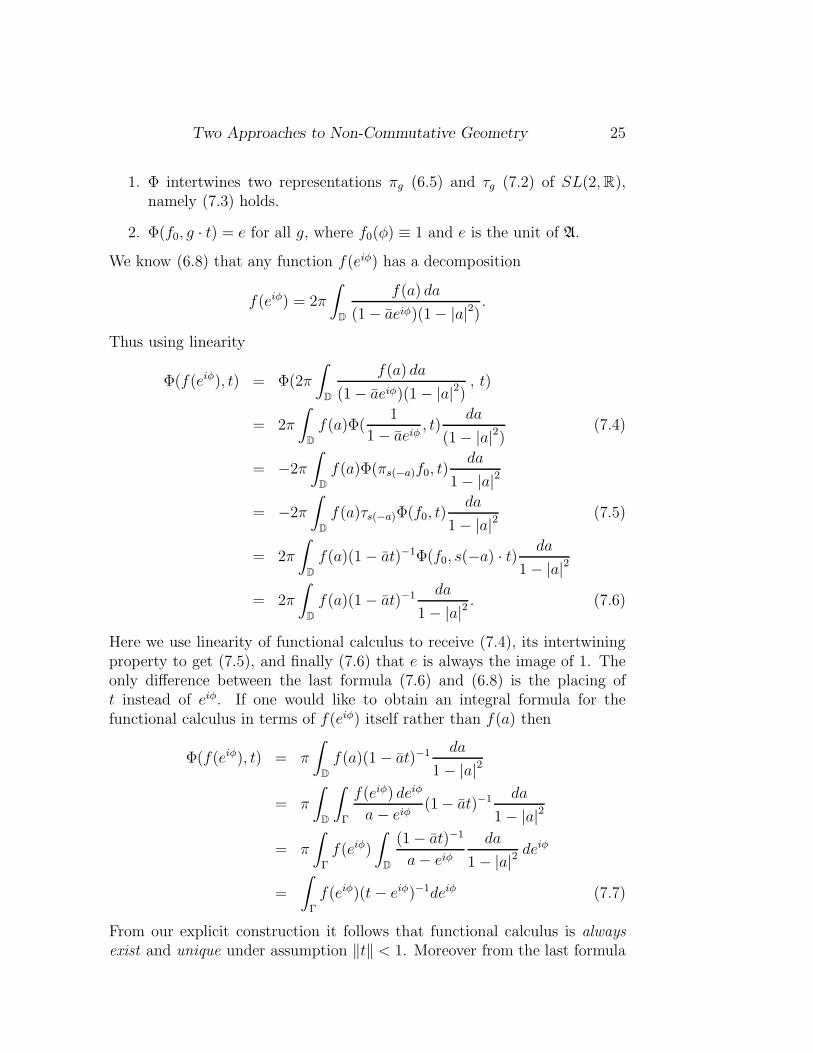
1. Φ intertwines two representations πg (6.5) and τg (7.2) of SL(2,R),namely (7.3) holds.

2. Φ(f0, g · t) = e for all g, where f0(φ) ≡ 1 and e is the unit of A.

We know (6.8) that any function f(eiφ) has a decomposition

f(eiφ) = 2π

∫

D

f(a) da

(1− aeiφ)(1− |a|2).

Thus using linearity

Φ(f(eiφ), t) = Φ(2π

∫

D

f(a) da

(1− aeiφ)(1− |a|2), t)

= 2π

∫

D

f(a)Φ(1

1− aeiφ, t)

da

(1− |a|2)(7.4)

= −2π

∫

D

f(a)Φ(πs(−a)f0, t)da

1− |a|2

= −2π

∫

D

f(a)τs(−a)Φ(f0, t)da

1− |a|2(7.5)

= 2π

∫

D

f(a)(1− at)−1Φ(f0, s(−a) · t)da

1 − |a|2

= 2π

∫

D

f(a)(1− at)−1 da

1− |a|2. (7.6)

Here we use linearity of functional calculus to receive (7.4), its intertwiningproperty to get (7.5), and finally (7.6) that e is always the image of 1. Theonly difference between the last formula (7.6) and (6.8) is the placing oft instead of eiφ. If one would like to obtain an integral formula for thefunctional calculus in terms of f(eiφ) itself rather than f(a) then

Φ(f(eiφ), t) = π

∫

D

f(a)(1− at)−1 da

1− |a|2

= π

∫

D

∫

Γ

f(eiφ) deiφ

a− eiφ(1− at)−1 da

1− |a|2

= π

∫

Γ

f(eiφ)

∫

D

(1− at)−1

a− eiφda

1− |a|2deiφ

=

∫

Γ

f(eiφ)(t− eiφ)−1deiφ (7.7)

From our explicit construction it follows that functional calculus is always

exist and unique under assumption ‖t‖ < 1. Moreover from the last formula


it follows also that our functional calculus coincides with the Riesz-Dunfordone [15, § VIII.2].

Remark 7.2 Guided by the Erlangen program we constructed a functionalcalculus coincided with the classical Dunford-Riesz calculus. The formeris traditionally defined in terms of algebra homomorphisms, i.e., on theDescartes geometrical language. So two different approaches again lead tothe same answer.

If one compares epigraphs to Sections 5 and 7 then it will be evidently that thefunctional calculus based on group representations responds to “the searchfor generality and unification”. Besides a funny alternative to classic Riesz-Dunford calculus the given scheme give unified approach to a variety of ex-isting and yet to be discovered calculi [26, Remark 4.2]. We consider someof them in next Section in connections with physical applications.

8 Do We Need That Observables Form an

Algebra?

. . . Descartes himself thought that all of physics couldbe reduced to geometry.

M. Kline [29, § 15.6].

We have already mentioned that the development of non-commutativegeometry intimately connected with physics, especially with quantum me-chanics. Despite the fact that quantum mechanics attracted considerableefforts of physicists and mathematicians during this century we still havenot got at hands a consistent quantum theory. Unsolved paradoxes and dis-crepant interpretations are linked with very elementary quantum models. Asa solution to this frustrating situation some physicists adopt a motto thatscience is permitted to supply inconsistent models “as is” so far they givereasonable numerical predictions to particular experiments11. However otherresearchers still believe that there exists a difference between the standardsof scientific enterprise and software selling industry.

We will review some topics in quantization problem in connection with thetwo approaches to non-commutative geometry. Quantum mechanics begunfrom experiments clearly indicated that Minkowski four dimensional space-time could not describe microscopical structure of our world (on the other

11And even more strange: there exists a variety of “immortal” theories already contra-dicting to our experience, see for example the red shift problem in [41].


hand it is also unsuitable for macroscopic description and these two faults be-came connected [41]). A way out is searched in many directions: dimension-ality of microscopical space was raised to m > 4 dimensions, its discontinuitywas imposed, etc. These search is based on the following conclusion [42]:

From a quantum mechanical standpoint, the trust of these workswas that “space-time” was more logically not a primary conceptbut one derived from the algebra of “observables” (or operators).In its simplest form the idea was space-time might be, at a deeperlevel, the spectrum of an appropriate commutative subalgebrathat is invariant under the fundamental symmetry group.

The right algebra of quantum observables is often constructed from classicobservables by means of quantization. A summary of quantization problemcould be given as follows (see also [24, § 15.4] and Table 1). The principalobjects of classical mechanics in Hamiltonian formalism are:

1. The phase space, which is a smooth symplectic manifold M .

2. Observables are real functions on M and could be considered as ele-ments of a linear space or algebra.

3. States of a physical system are linear functionals on observables.

4. Dynamics of observables is defined by a Hamiltonian H and equation

F = H,F. (8.1)

5. Symmetries of the physical system act on observables or states viacanonical transformations of M .

Of course points of phase space is in one-to-one correspondence with states ofthe system and they together are completely defined by the set of observables.The later viewed as an algebra recovers M as its space of maximal ideals.Thus observables, dynamics, and symmetries are primary objects while phasespace and states could be restored from them.

The quantum mechanics has its parallel set of notions:

1. Phase space is the projective space P (V ) of a Hilbert space V .

2. Observables are self-adjoint operators on V .

3. States of a physical system defined by a vector ξ ∈ V , ‖ξ‖ = 1.


4. Dynamics of an observable F defined by a self-adjoint operator H viathe Heisenberg equation

˙F =

i~

2π[H, F ]. (8.2)

5. Symmetries of physical system act on observables or states via unitaryoperators on V .

Again we could start from an algebra of observables and then realize statesand Hilbert space V via GNS construction [24, § 4.3].

The similarity of two descriptions (with correspondence of the Poissonbracket and commutator) makes it very tempting to construct a map Q,which is called the Dirac quantization, such that

1. Q maps a function F to an operator F = Q(F ), i.e., classic observablesto quantum ones.

2. Q has an algebraic property F1, F2 = [F1, F2], i.e., maps the Poissonbrackets to the commutators.

3. Q(1) = I, i.e., the image of the function 1 identically equal to one isthe identity operator I.

Unfortunately, Q does not exists even for very simple cases. For example, the“no go” theorem of van Hove in [17] states that the canonical commutationrelations (4.1) could not be extended even for polynomials in X and Y ofdegree greater than 2.

As a solution one could try to select a primary set of classic observablesF1, . . . , Fn, which defines coordinates on M and thus any other observableF is a function of F1, . . . , Fn: F = F (F1, . . . , Fn). For such a small setof observables a quantization Q always exists (for example the geometric

quantization [24, § 15.4]) and one could hope to construct general quantum

observable F as a function of the primary ones F = F (F1, . . . , Fn).But to do that one should answer the question equivalent to functional

calculus: What is a function of n operators? For a commuting set of oper-ators as well as for the case n = 1 it is easy to give an answer in terms ofalgebra homomorphisms : the functional calculus Φ is an algebra homomor-phism from an algebra of function to an algebra of operators, which is fixedby a condition Φ(Fi) = Fi, i = 1, . . . , n. But for physically interesting case

of several non-commuting Fi this way is impossible.Several solutions were given whether analytically by integral formulas like

for the Feynman [16] and Weyl [2] calculi or algebraically by “ordering rules”


like for the Wick [43, § 6] and anti-Wick [5] calculi. These approaches areconnected: if calculus is defined via integral formula then it correspond tosome ordering (e.g., the Feynman case) or symmetrization (e.g., the Weylcase); and vise versa starting from particular ordering a suitable integralrepresentation could be found [5].

We will consider the Weyl functional calculus in more details. Let T =Tj, j = 1, . . . , n be a set of bounded selfadjoint operators. Then for everyset ξj of real numbers the unitary operator exp(i

∑n1 ξjTj) is well defined.

The Weyl functional calculus [2] is defined by the formula

f(T) =

∫

Rn

exp

(i

n∑

1

ξjTj

)f(ξ) dξ, (8.3)

where f(ξ) is usual Fourier transform of f(x). In [2] the following propertiesof the Weyl calculus were particularly proved:

1. The image of a polynomial p(x) is the symmetric in Tj polynomial p(T)(e.g. image of p(x1, x2) = x1x2 is p(T1, T2) =

12(T1T2 + T2T1)).

2. The Weyl calculus commutes with affine transformations, i.e., let Si =∑nj=1mijTj for a nonsingular matrix mij, then

f(S) = g(T) where g(x) = f(m · x). (8.4)

Moreover the last condition together with the requirement that Weyl func-tional calculus gives the standard functional calculus for polynomials in onevariable completely defines it. We know that functional calculus for one vari-able could be also defined by its covariance property. Thus we could give anequivalent definition12

Definition 8.1 The Weyl functional calculus for an n-tuple T of selfadjointoperators is a linear map from a space of functions on Rn to operators in aC∗-algebra A such that

1. Intertwines two representation of affine transformation, namely (8.4)holds.

2. Maps the function eix1 on R to operator

eiT1 =∑ (iT1)

n

n!. (8.5)

12We skip details because the problem is beyond the L2 scope presented in the paper.


While the affine group is natural for Euclidean space one could needother groups under different environments. For example, one could con-sider a non-commutative geometry generated by the group of conformal (orMobius) transformations. It is known [9] that the group M of Mobius (map-ping spheres onto spheres) transformations of Rn could be represented viafraction-linear transformations with the help of Clifford algebras Cℓ(n). Tak-ing the tensor product A = A⊗ Cℓ(n) of an operator algebra A and Cliffordalgebra we could consider a representation of conformal group M in thenon-commutative space A, which also is defined by fraction-linear transfor-mations.

Such an approach leads particularly to a natural definition of joint spec-trum of n-tuples of non-commuting operators and a functional calculus ofthem [26]. The functional calculus is not an algebra homomorphism (forn > 1) but is an intertwining operator between two representations of con-formal group M . Nevertheless the joint spectrum obeys a version of thespectral mapping theorem [26].

It is naturally to expect that physically interesting functional calculi fromgroup representations are not restricted to two given examples. Lookingon these functional calculi as on a quantization one found that commoncontradiction between the group covariance and an algebra homomorphismproperty vanishes (as the algebra homomorphism property itself). It turnsthat the group covariance alone is sufficient for the definition of functionalcalculus. Moreover such an approach gives a unified description of all knownfunctional calculi and suggests new ones.

One should be aware that algebraic structure it still important: it entersto the definition of the group action via fraction-linear transformations (7.2)or definition of exponent (8.5). So the question posed at the title of Sectionmight have an answer: Yes, we need that observables form an algebra, but

we do not need that quantization will be connected with an algebra homomor-

phism property in general.

9 ConclusionWe often hear that mathematics consists mainly in“proving theorems”. Is a writer’s job mainly that of“writing sentences”?

G.-C. Rota [21, Chap. 11].

Looking through the present discussion one could not resist to the follow-ing feeling:

The goal of new mathematical facts is to elaborate the true language for

an understanding old ideas, such that they will be expressed with the ultimate


perfectness.

This goal could not be obviously accomplished within a finite time. Sowe have a good reason for self-irony mentioned at the end of Introduction.

10 Acknowledgments

The paper was written while the author stay at the Department of Mathe-matical Analysis, University of Gent, as a Visiting Postdoctoral Fellow of theFWO-Vlaanderen (Fund of Scientific Research-Flanders), Scientific ResearchNetwork “Fundamental Methods and Technique in Mathematics” 3GP03196,whose hospitality and support I gratefully acknowledge.

I would like to thank to Prof. I.E. Segal and Yu. Manin for usefulremarks on the subject. I am also grateful to Dr. A.A. Kirillov, Jr. forcritical discussion, which allows to improve presentation in Section 4.

In the paper we try to establish some connections between several areasof algebra, analysis, and geometry. A reasonable bibliography to such apaper should be necessary incomplete and the given one is probably even notrepresentative. Any suggestions about unpardonable omitted references willbe thankfully accepted.

References

[1] S. Twareque Ali, J.-P. Antoine, J.-P. Gazeau, and U.A. Mueller. Coherentstates and their generalizations: A mathematical overview. Rev. Math. Phys.,7(7):1013–1104, 1995. Zbl # 837.43014.

[2] Robert F. V. Anderson. The Weyl functional calculus. J. Funct. Anal., 4:240–267, 1969.

[3] Michael Atiyah and Wilfried Schmid. A geometric construction of the discreteseries for semisimple Lie group. In J.A. Wolf, M. Cahen, and M. De Wilde,editors, Harmonic Analysis and Representations of Semisimple Lie Group,volume 5 of Mathematical Physics and Applied Mathematics, pages 317–383.D. Reidel Publishing Company, Dordrecht, Holland, 1980.

[4] V. Bargmann. On a Hilbert space of analytic functions and an associatedintegral transform. Part I. Comm. Pure Appl. Math., 3:215–228, 1961.

[5] Felix A. Berezin. Method of Second Quantization. “Nauka”, Moscow, 1988.(Russian).


[6] F. Brackx, R. Delanghe, and F. Sommen. Clifford Analysis, volume 76 of Re-search Notes in Mathematics. Pitman Advanced Publishing Program, Boston,1982.

[7] Ali Chamseddine and Alain Connes. The spectral action principle. Commun.Math. Phys, 186(3):731–750, 1997. preprint hep-th/9606001.

[8] Wendy Chan, Gian-Carlo Rota, and Joel A. Stein. The power of positivethinking. In Invariant Methods in Discrete and Computational Geometry.Proceedings of the conference held in Curacao, June 13–17, 1994, pages 1–36.Kluwer Academic Publishers, Dordrecht, 1995.

[9] Jan Cnops. Hurwitz Pairs and Applications of Mobius Transformations. Ha-bilitation dissertation, Universiteit Gent, Faculteit van de Wetenschappen,1994. ftp://cage.rug.ac.be/pub/clifford/jc9401.tex.

[10] Jan Cnops and Vladimir V. Kisil. Monogenic functions and representationsof nilpotent lie groups in quantum mechanics. 1997. (In preparation).

[11] Lewis A. Coburn. Berezin-Toeplitz quantization. In Algebraic Mettods inOperator Theory, pages 101–108. Birkhauser Verlag, New York, 1994.

[12] Alain Connes. Non-Commutative Geometry. Academic Press, New York,1994.

[13] Ingrid Daubechies. Ten Lectures on Wavelets, volume 61 of CBMS-NSF Re-gional Conference Series in Applied Mathematics. Society for Industrial andApplied Mathematics (SIAM), Philadelphia, PA, 1992.

[14] Ronald G. Douglas. Banach Algebra Techniques in Operator Theory, vol-ume 49 of Pure and Applied Mathematics. Academic Press, Inc., New York,1972.

[15] Nelson Dunford and Jacob T. Schwartz. Linears Operators. Part I: GeneralTheory, volume VII of Pure and Applied Mathematics. John Wiley & Sons,Inc., New York, 1957.

[16] Richard P. Feynman. An operator calculus having applications in quantumelectrodynamics. Phys. Rev. A (3), 84(2):108–128, 1951.

[17] Gerald B. Folland. Harmonic Analysis in Phase Space. Princeton UniversityPress, Princeton, New Jersey, 1989.

[18] John E. Gilbert and Margaret A.M. Murray. Clifford Algebras and DiracOperators in Harmonic Analysis, volume 26 of Cambridge Studies in AdvancedMathematics. Cambridge University Press, Cambridge, 1991.


[19] Roger Howe. On the role of the Heisenberg group in harmonic analysis. Bull.Amer. Math. Soc. (N.S.), 3(2):821–843, 1980.

[20] Roger Howe and Eng Chye Tan. Non-Abelian Harmonic Analysis: Applica-tions of SL(2,R). Universitext. Springer-Verlag, New York, 1992.

[21] Mark Kac, Gian-Carlo Rota, and Jacob T. Schwartz. Discrete Thoughts:Essays on Mathematics, Science, and Philosopy. Birkhauser Verlag, Boston,1992.

[22] Christian Kassel. Quantum Groups, volume 155 of Graduate Text in Mathe-matics. Springer-Verlag, New York, 1994.

[23] A. A. Kirillov and A. D. Gvishiani. Theorems and Problems in FunctionalAnalysis. Problem Books in Mathematics. Springer-Verlag, New York, 1982.

[24] Alexander A. Kirillov. Elements of the Theory of Representations, volume220 of A Series of Comprehensive Studies in Mathematics. Springer-Verlag,New York, 1976.

[25] Vladimir V. Kisil. Integral representation and coherent states. Bull. Belg.Math. Soc. Simon Stevin, 2(5):529–540, 1995.

[26] Vladimir V. Kisil. Mobius transformations and monogenic functional calculus.ERA of Amer. Math. Soc., 2(1):26–33, August 1996.

[27] Vladimir V. Kisil. Analysis in R1,1 or the principal function theory. page 25,1997. E-print funct-an/9712003, clf-alg/kisi9703.

[28] John R. Klauder and Bo-Sture Skagerstam, editors. Coherent States. Appli-cations in physics and mathematical physics. World Scientific Publishing Co.,Singapur, 1985.

[29] Morris Kline. Mathematical Thought from Ancient to Modern Times. OxfordUniversity Press, New York, 1972.

[30] A.W. Knapp and N.R. Wallach. Szego kernels associated with discrete series.Invent. Math., 34(2):163–200, 1976.

[31] Donald E. Knuth. The TEXbook. Addison-Wesley, Reading, Massachusetts,1986.

[32] Adam Koranyi. Harmonic functions on symmetric spaces. In William M.Boothby and Guido L. Weiss, editors, Symmetric Spaces: Short Courses Pre-sented at Washington University, volume 8 of Pure and Applied Mathematics,pages 379–412. Marcel Dekker, Inc, New York, 1972.

[33] Steven G. Krantz. Function Theory of Several Complex Variables. Pure andApplied Mathematics. John Wiley & Sons, New York, 1982.


[34] Serge Lang. SL2(R), volume 105 of Graduate Text in Mathematics. Springer-Verlag, New York, 1985.

[35] Yuri I. Manin. Quantum Group and Non-Commutative Geometry. Universitede Monreal, Centre de Recherches Mathematiques, Monreal, PQ, 1988.

[36] Yuri I. Manin. Topics in Noncommutative Geometry. Princeton UniversityPress, Princeton, New Jersey, 1991.

[37] A. M. Perelomov. Generalized Coherent States and Their Applications.Springer-Verlag, Berlin, 1986.

[38] Walter Rudin. Function Theory in the Unit Ball of Cn. Springer-Verlag, NewYork, 1980.

[39] Lew I. Sabinin. Loop geometries. Math. Notes, 12:799–805, 1972.

[40] Irving E. Segal. Mathematical Problems of Relativistic Physics, volume II ofProceedings of the Summer Seminar (Boulder, Colorado, 1960). AmericanMathematical Society, Providence, R.I., 1963.

[41] Irving E. Segal. The mathematical implications of fundamental physical prin-ciples. In The Legacy of John v. Neumann (Providence, 1990), volume 50 ofProc. Sympos. Pure Math., pages 151–178. American Mathematical Society,Providence, R.I., 1990.

[42] Irving E. Segal. Book review. Bull. Amer. Math. Soc. (N.S.), 33(4):459–465,1996. Review on book [12].

[43] Irving E. Segal. Rigorous covariant form of the correspondence principle.In William Arveson et al., editor, Quantization, Nonlinear Partial Differen-tial Equations, and Operator Algebra (Cambridge, MA, 1994), volume 59 ofProc. Sympos. Pure Math., pages 175–202. American Mathematical Society,Providence, R.I., 1996.

[44] Michael E. Taylor. Noncommutative Harmonic Analysis, volume 22 of Math.Surv. and Monographs. American Mathematical Society, Providence, R.I.,1986.

arxiv:funct-an/9703001v3 6 feb 1998funct-an/9703001v3 6 feb 1998 preprint funct-an/9703001, 1997 two...

Documents