arxiv:hep-ph/0411274v1 20 nov 2004
TRANSCRIPT
arX
iv:h
ep-p
h/04
1127
4v1
20
Nov
200
4
February 2, 2008 1:28 Proceedings Trim Size: 9in x 6in lectures
TASI LECTURES ON NEUTRINO PHYSICS
ANDRE DE GOUVEA
Northwestern University, Department of Physics & Astronomy
2145 Sheridan Road,
Evanston, IL 60208, USA
e-mail: [email protected]
I discuss, in a semi-pedagogical way, our current understanding of neutrino physics.I present a brief history of how the neutrino came to be “invented” and observed,and discuss the evidence that led to the recent discovery that neutrinos changeflavor. I then spend some time presenting mass-induced neutrino flavor change(neutrino oscillation), and how it pieces all the neutrino puzzles except for theLSND anomaly, which is also briefly discussed. I conclude by highlighting theimportance of determining the nature of the neutrinos, i.e., are they Dirac orMajorana fermions.
NUHEP-TH/04-17
1. Introduction
Neutrino physics is among the most exciting and active areas of research
in high energy physics, both experimentally and theoretically. No other
area of particle physics research has gone through as dramatic a transfor-
mation, and one can arguably claim that the near and intermediate future
of research associated with neutrinos is very bright indeed.
The reason for all the excitement is the fact that a plethora of neutrino
detectors have obtained, without a shadow of a doubt, the only palpable
evidence for physics beyond the standard model of eletroweak interactions.
New physics seems to have manifested itself in the form of neutrino masses
and lepton mixing.
Here, I discuss not only what we know (and don’t know) about neutrino
properties and interaction, but also spend some time exploring how these
were uncovered experimentally and theoretically. In Sec. 2, I present a
condensed history of the neutrino, including how they were discovered, first
theoretically, and then experimentally, and when we started suspecting that
1

February 2, 2008 1:28 Proceedings Trim Size: 9in x 6in lectures
2
there was something wrong with the naive standard model description of
neutrino properties. In Sec. 3, I discuss in some detail the phenomenon of
neutrino oscillations, and describe how oscillations were used to solve almost
all long-standing neutrino puzzles in Sec. 4. Sec. 5 contains a brief digression
on the still-unresolved LSND anomaly. Finally, in Sec. 6, I summarize what
we have learned from neutrinos, what I mean by “neutrinos provide the
only palpable evidence of physics beyond the standard model,” and what
we think this new physics is.
Before proceeding, two comments. (i) In response to the rapid meta-
morphosis of neutrino physics, several excellent overviews and pedagogical
lecture notes have been written and made available to the community,1,2,3
and these discuss at different levels of detail and rigor everything contained
here. I hope that this “historical approach” to the subject adds to the
literature, which is quite excellent. (ii) I apologize in advance for all in-
accuracies regarding historical facts and the omission of several important
references.
2. Beta-Rays and Missing Neutrinos
Here I review, in a very biased, simplified, and condensed form, the his-
tory of weak interactions and neutrino physics. Not only is it a fascinating
subject, but it also serves to illustrate that neutrinos have always managed
to challenge and confuse physicists into contemplating what was once per-
ceived to be impossible and questioning fundamental principles and theoret-
ical biases. Over the years, neutrinos have provided fundamental clues that
lead to significant progress in the understanding of fundamental physics. I
also wish to make the point that progress in neutrino research had always
been very slow, in contrast to the boom observed in the past six years. I
refer readers to Ref. 3 for a detailed overview of the history of neutrinos.
I also summarize the series of experimental results that lead to the
discovery that neutrinos can change flavor, hence changing in qualitative
way our understanding of them.
2.1. Biased Neutrino History
The history of the neutrinoa is strongly tied to the history of the once
very mysterious weak interactions. These were “stumbled upon,” quite
accidently, by Henri Becquerel in 1896, one year before the electron was
aMost of the material discussed in this subsection was obtained from Ref. 3.

February 2, 2008 1:28 Proceedings Trim Size: 9in x 6in lectures
3
discoverd by J.J. Thompson and several years before nuclei were known to
exist. All pioneering studies of natural radioactivity also took place years
before the development of even the most rudimentary aspects of quantum
mechanics.
Becquerel is credited with the discovery that, even in the absence of an
outside stimulus (e.g. light, electricity) some chemical elements naturally
emit radiation capable, for example, of leaving a mark in a photographic
plate. In the early 1900’s, detailed analysis of this natural radioactivity
revealed that different elements emitted different types of radiation, and
these were baptized, by Lord Rutherford, α, β, and γ radiation, or rays.
The different types of radiation possessed rather distinct properties, and it
is curious to note, in hindsight, that each was due to a different interaction
(α → strong, β → weak, γ → electromagnetic):
• α-rays were easy to absorb and bent slightly (positive charge,
“heavy”) in the presence of magnetic fields. It was discovered,
due to their absorption properties, that α-rays emitted from a well
defined isotope were mono-energetic;
• β-rays were harder to absorb than α-rays, and they bent signifi-
cantly (negative charge, “light”) in the presence of magnetic fields;
• γ-rays did not bent in the presence of magnetic fields (no charge),
and were very hard to absorb.
2.1.1. The Nuclear β-Decay Spectrum
The pre-history of the neutrino begins with detailed studies of β radia-
tion. Progress in the understanding of β-rays was very slow and rather
“tortuous.”
Early studies revealed that β-rays were identical to cathode rays (elec-
trons), and that their spectrum was discrete, like the spectrum of α-
radiation. While the former is correct, the later incorrect understanding
was obtained from two distinct pieces of evidence: (i) studies of the ab-
sorption of β-rays seemed to indicate that these were mono-energetic, and
(ii) the spectrum of a β-ray beam in the presence of a constant magnetic
field incident on a photographic plate seemed to be discrete, and hence
indicative that the β-beam was composed of several discrete components,
each with a different, well-defined energy.
Evidence (i) was shown to be incorrect for “theoretical reasons.” It
turned out that the phenomenology used to describe β-ray absorption was
wrong. It was established that, contrary to initial prejudice, electrons and
February 2, 2008 1:28 Proceedings Trim Size: 9in x 6in lectures
4
α-particles do not lose energy while propagating inside matter in the same
way. Evidence (ii) was also incorrect, this time for “experimental reasons.”
It turned out that photographic plates were not the best detector technology
to observe the β-ray spectrum!
In 1914, Chadwick, using more advanced detection techniques, pre-
sented definitive evidence that the observed β-ray spectrum was contin-
uous. It remained to determine whether the primordial spectrum was also
continuous or whether it was originally discrete but somehow modified in
its way from the material to the detector. Several hypothetical energy-
loss mechanisms were raised, including interactions of the β-radiation with
atomic electrons, or interactions with other types of radiation, including
γ-rays.b It was only fifteen years after Chadwick’s discovery that the issue
was experimentally settled: the nuclear β-ray spectrum is continuous. And
no-one had any idea why that would be the case.
It is important to appreciate that it took over thirty years to establish
that the β-ray spectrum was continuos, and that the theoretical prejudice
of the time was that the spectrum should be discrete. The reasons behind
the incorrect preconceived idea are easy to understand. First, β-radiation
was a quantum mechanical phenomenon, and quantum mechanical spectra
were discrete (e.g. atomic spectra). Second of all, the β-radiation phe-
nomenon was described by AZ →A (Z + 1) + e−, where AZ is a nucleus
with atomic number Z and mass number A. Energy and momentum con-
servation dictate that, modulo finite temperature effects (small, calculable),
the electrons leave the nucleus with a fixed, well-defined energy, given by
the mass difference between the parent and daughter nuclei. It seemed, at
the time, that, in order to understand continuous nuclear β-decay spectra,
one was required to give up the principle of conservation of energy!
2.1.2. 1920’s Nuclear Physics
Of course, the early third of the twentieth century was not without its
share of other fundamental physics puzzles. One was associated with un-
derstanding the nucleus and its constituents, and apparent contradictions
of the spin-statistics theorem. In early nuclear physics, it had been pos-
tulated that nuclei were made up of protons and electrons, such that AZ
contained A protons and A−Z electrons (such that the nuclear charge was
bMost β-ray emitters also emit γ-rays.

February 2, 2008 1:28 Proceedings Trim Size: 9in x 6in lectures
5
Z).c For example, an 4He nucleus was to be composed of four protons and
two electrons, while 14N= 14p + 7e−.
There were several fundamental problems with this model for the nu-
cleus. One was related to the magnetic moment of nuclei. It was well
known at the time that the electron magnetic moment was much larger
than the proton one, and also much larger then the nuclear one. How
was that possible, if the nucleus was a collection of protons and electrons?
Worse, perhaps, was the fact that the spin-statistics theorem seemed to be
violated: according to the proton+electron nuclear model, 14N is predicted
to be a collection of an odd number of fermions (14+7=21), which would
mean it should have a half-integer spin and hence behave like a fermion.
Experiments had revealed, however, that 14N was a boson.
Short of assuming that the above model for the nucleus was simply
wrong (which turned out to be the case), there were only a few possible
solutions to the puzzles raised above. One “common theme” to all the puz-
zles was that nuclear-bound electrons did not behave like unbound ones.
At around 1929–1930, Niels Bohr contemplated the possibility that nuclear
electrons not only did not behave as ordinary fermion but also interacted
in a way that violated energy and momentum conservation, as was required
to explain the continuous spectrum of β-decay. Far from considered crazy,
Bohr’s idea made it to the mainstream realm of textbooks: “This would
mean that the idea of energy and its conservation fails in dealing with pro-
cesses involving the emission or capture of nuclear electrons. This does
not sound improbable if we remember all that has been said about peculiar
properties of electrons in the nucleus.”4
2.1.3. Pauli’s Neutron Hypothesis
Wolfgang Pauli came to the rescue in December, 1930, when he raised the
hypothesis that there was a third constituent inside the nucleus. In his noto-
rious letter addressed to the participants of a nuclear physics conference in
Tubingen, Germany, included in summarized form below, Pauli postulated
the existence of what he called a ‘neutron,’ a fermion with no charge which
interacted very weakly with matter and weighed less than 1% of the proton
mass. The presence of the neutron saved the spin-statistics theorem (e.g.14N= 14p+7e−+7‘ν’, a boson) and explained the apparent violation of en-
cThere were more complicated models for the nucleus at the time which included, forexample, α-particles as fundamental nuclear constituents.

February 2, 2008 1:28 Proceedings Trim Size: 9in x 6in lectures
6
ergy conservation in β-decay. He assumed that AZ →A(Z +1)+e−+‘ν’ was
the correct physical process and, since the final state contained three bod-
ies, not only was the electron energy spectrum continuous, but the maximal
electron energy was guaranteed to be always less than the parent–daughter
mass-difference. It is, perhaps, also noteworthy to mention that Pauli did
not publish his idea until several years later. He was worried about the
fact that he could be postulating a new particle, whose existence would
never be verified experimentally, in order to save a handful of theoretical
principles. . .
Dear Radioactive Ladies and Gentlemen,
I have come upon a desperate way out regarding the wrong statistics
of the 14N and 6Li nuclei, as well as the continuous β-spectrum, in
order to save the “alternation law” statistics and the energy law. To
wit, the possibility that there could exist in the nucleus electrically
neutral particles, which I shall call “neutrons,” and satisfy the ex-
clusion principle... The mass of the neutrons should be of the same
order of magnitude as the electron mass and in any case not larger
than 0.01 times the proton mass. The continuous β-spectrum would
then become understandable from the assumption that in β-decay
a neutron is emitted along with the electron, in such a way that the
sum of the energies of the neutron and the electron is constant. . .
For the time being I dare not publish anything about this idea and
address myself to you, dear radioactive ones, with the question how
it would be with experimental proof of such a neutron, if it were to
have the penetrating power equal to about ten times larger than a
γ-ray.
I admit that my way out may not seem very probable a priori since
one would probably have seen the neutrons a long time ago if they
exist. But only the one who dares wins, and the seriousness of the
situation concerning the continuous β-spectrum is illuminated by
my honored predecessor, Mr Debye who recently said to me in Brus-
sels: “Oh, it is best not to think about this at all, as with new taxes.”
One must therefore discuss seriously every road to salvation. Thus,
dear radioactive ones, examine and judge. Unfortunately, I cannot
appear personally in Tubingen since a ball. . . in Zurich. . . makes my
presence here indispensible. . . .
Your most humble servant, W. Pauli
Adapted summary of an English Translation to Pauli’s letter dated
December 4, 1930, from Ref. 3.

February 2, 2008 1:28 Proceedings Trim Size: 9in x 6in lectures
7
2.1.4. The Neutron and the Neutrino, the Muon and the Pion
A few of years later, Chadwick discovered a neutral nuclear constituent. By
studying the properties of the neutral radiation n emitted in the process9Be+α →12C+n, he found out that this so-called neutron was a deeply
penetrating neutral particle slightly heavier than the proton, quite distinct
from γ-rays. This was not the neutron postulated by Pauli, but a different
particle all together. Given the fact that Chadwick’s neutron was much
heavier than Pauli’s one, Fermi renamed Pauli’s neutron the ‘neutrino.’d
More than baptizing the neutrino, Fermi wrote down, in 1934, a new
quantum mechanical description of the weak interactions. He postulated
that β-decay was mediated by the decay process n → pe−νe,e which was
described by the following four-fermion interaction:f
GF√2
(nΓNp) (νeΓLe) + H.c., (1)
where GF is a dimensionful constant that characterizes the strength of
the interaction (the Fermi constant), and ΓN,L are linear combinations
of “gamma matrices” 1, γ5, γµ, γµγ5, σµν , which were to be determined by
more precise measurements of weak interaction processes. With this new
understanding of the β-decay process, a much improved picture of the nu-
cleus was built. Nuclei were built out of nucleons (neutrons and protons)
— AZ = Zp + (A−Z)n, a concept which correctly explained the magnetic
moment of the nuclei, and allowed one to determine, correctly, whether a
given nucleus was a boson or a fermion (e.g. 14N= 7p + 7n, a boson).
Eq. (1) not only provided a mathematical description of nuclear beta
decay, but also allowed one to compute the cross-section for other related
physical processes, including
νe + p → e+ + n, (2)
which was crucial, many years later, to determine whether neutrinos could
be experimentally observed. I will return to this issue shortly.
The importance of the Fermi theory and our understanding of the weak
interactions increased tremendously in the years that followed. In 1936, a
dIn italian, the suffix ‘ino’ is used to represent the diminutive — ‘neutrino’ = ‘smallneutron.’eI will use modern notation for neutrinos and antineutrinos henceforth, in order to avoidmore confusion.fAgain, I use modern field theory notation to avoid confusion.

February 2, 2008 1:28 Proceedings Trim Size: 9in x 6in lectures
8
new elementary particle, the µ ‘meson’ was discovered in cosmic ray ex-
periments. This particle, now known as the muon (a lepton), was first
confused with the pion, postulated by Hideki Yukawa to be the mediator
of the interaction responsible for binding protons and neutrons inside the
nucleus. This particular issue was resolved theoretically in 1947 by Mar-
shak and Bethe with the “two meson hypothesis.” Their proposal was later
confirmed to be correct when pions were first observed in cosmic ray ex-
periments, also in 1947. As far as neutrinos are concerned, it is important
to note that it was established that
π+ → µ+νµ, (3)
µ+ → e+νeνµ, (4)
and that both the pion and muon decay rates were characterized by the
same interaction strength which was found in nuclear decay processes,
Eq. (1). For example, the four-fermion operator
GF√2
(νµΓµ) (νeΓe) + H.c., (5)
mediates Eq. (4). The fact that GF in Eq. (1), is the same as GF in
Eq. (5) was the first indication that the weak interactions were a universal
phenomenon, much like electromagnetism, and not an exclusive property
of nuclear systems.
A very long, eventful time passed between Fermi’s formulation of the
weak interactions and the confirmation that Eq. (1) was correct beyond any
reasonable doubt plus the experimental determination of the nature of the
ΓN ’s. I refer readers to, e.g., Ref. 3 and references therein for a detailed
description. Of particular importance were precision studies of the energy
spectrum of electrons emitted in muon decay (so-called Michel electrons)
and searches for the helicity suppressed π+ → e+νe decay, finally observed
for the first time in 1958. A couple of years before that, weak interac-
tions caused a significant amount of commotion in the community with the
hypothesis, by Lee and Yang, and subsequent experimental confirmation,
first by Wu et al, and a little later by Garwin, Lederman, and Weinrich,
and by Friedman and Telegdi, that parity was maximally violated in weak
processes. The whole issue was finally settled in the same year, thanks to
theoretical developments by Marshak and Sudarshan and Feyman and Gell-
mann, which argued in favor of the now well known V − A (or γµ − γµγ5)
structure of the weak interactions.
The purely left-handed structure of the leptonic charged current
(νeγµ(1−γ5)e), combined with the fact that neutrino masses were known to

February 2, 2008 1:28 Proceedings Trim Size: 9in x 6in lectures
9
be much smaller than the electron mass, allowed for a very compact descrip-
tion of the neutrino. A free, massive spin 1/2 particles is characterized, not
surprisingly, by its mass m, its total spin s the value of its spin projection
in a specific direction, sz. One particularly useful direction for measuring
the particle’s spin is its direction of motion p, in which case sz is called the
particle’s handedness, or helicity. If ~s · p|m, s〉 = +1/2|m, s〉 (−1/2|m, s〉),the particle is said to be right-handed (left-handed). The helicity is not
reference-frame independent in the case of massive particles. This is easy
to see. If the particle is massive, one can always choose to change into a
reference frame moving along its direction with a larger velocity. In this
case, p ↔ −p, while ~s ↔ ~s, such that, say, a right-handed state is now
viewed as a left-handed one.
In the case of massless fermions, however, the helicity is a good quan-
tum number, independent on the reference frame. The smallest number
of degrees of freedom a massless fermion field can describe is, hence, two:
a left-handed (or right-handed) fermion, plus its CPT-transform, a right-
handed (or left-handed) antifermion.g Because the weak-interactions are
purely left-handed, this has proven, so far, to be enough to describe the
neutrinos.
One of the most dramatic manifestations of this phenomenon is the
fact that muons emitted in pion decay at rest are virtually 100% polarized.
This is a consequence of the fact that the weak interactions are purely
left-handed, and that the neutrino mass is, at most, tiny:
π+ → µ+Lνµ,L ALWAYS; (6)
↓ (P )
π+ → µ+Rνµ,R NEVER; (7)
↓ (C)
π− → µ−Rνµ,R ALWAYS; (8)
↓ (P )
π− → µ−L νµ,L NEVER. (9)
In summary, in the absence of neutrino masses and new interactions beyond
SU(2)L, right-handed neutrinos and left-handed antineutrinos can never be
produced or detected. This is equivalent to saying they don’t exist.
gThis is to be contrasted to the case of charged, masssive fermions which require four de-
grees of freedom (e.g., the left-handed electron and its CPT-transform, the right-handedpositron, plus its “Lorentz transform” the right-handed electron and CPT-transform,the left-handed positron). See Ref. 5 for a more detailed discussion of this point.
February 2, 2008 1:28 Proceedings Trim Size: 9in x 6in lectures
10
Before proceeding, I’ll mention that the neutrino helicity was first de-
termined in 1958 by Goldhaber et al. in a very elegant experiment. They
produced neutrinos via e−+152Eu→ νe+152Sm∗(J = 1). The excited
state of samarium decayed very quickly by emitting a γ-ray, 152Sm∗(J =
1) →152Sm(J = 0) + γ. Conservation of energy and momentum forces the
photon and the neutrino to be back-to-back, while conservation of angu-
lar momentum correlates the neutrino helicity to the photon polarization.
Goldhaber et al. established that the photons produced in these processes
were, within errors, 100% polarized, and that the neutrinos were purely
left-handed.
2.1.5. Direct Detection of (Anti)Neutrinos
While the neutrino was postulated to exist in 1930 and widely accepted to
be a real particle shortly thereafter, it was not until the 1950’s that the
necessary means for detecting neutrinos became available. As mentioned
earlier, Fermi theory allowed one to compute the neutrino–nucleon cross
section, and hence estimate the neutrino flux and detector size required to
statistically observe neutrino-induced events.
In the early 1950’s “Project Poltergeist,” headed by Frederick Reynes
and Clyde Cowan, got started. Its mission was to detect neutrinos. It
took advantage of the technological developments which took place in the
1940’s in order to develop the fission bomb. Curiously enough, one of the
first proposals consisted of measuring the (very high) instantaneous flux
of antineutrinos emitted during an atomic bomb explosion (remember that
nuclear tests in the american desert were taking place at the time!). One of
the down sides of this particular setup included the fact that the experiment
needed to be located rather close to the site of the explosion — not the most
stable of places to house a detector!
This rather original idea — never implemented — was substituted with
the idea to measure the antineutrino flux produced by nuclear power reac-
tors. Nuclear reactors were also a “bi-product” of the bomb, and were used
to enrich heavy isotope samples. While the instantaneous antineutrino flux
from nuclear reactors was much less than the one generated during a nuclear
explosion, the integrated flux could be much larger — and the experimental
conditions were, of course, much more sensible.
In order to successfully detect neutrino-induced interactions, it was cru-
cial to separate these from background events due to cosmic rays, radioac-
tivity in the detector and surrounding material, etc. This was accomplished

February 2, 2008 1:28 Proceedings Trim Size: 9in x 6in lectures
11
successfully in the following way. Antineutrinos interact with protons as de-
picted in Eq. (2). The daughter positron quickly annihilates with a near-by
electron
e+e− → γγ, (10)
and the photon energy is detected in some scintillating environment (fur-
thermore, the total deposited energy is related to the positron energy, which
is related to the incoming antineutrino energy). While the positron is be-
ing annihilated, the recoil neutron random walks inside the detector and
is absorbed, after a well defined characteristic time, emitting γ-rays with
well-defined energy. The coincidence between the first signal (due to the
elelctron-positron annihilation) and second one, a well-defined amount of
time afterwards, was crucial to the success of Project Poltergeist, and is
used to this very day to study antineutrinos produced in nuclear reactors.
The first hint of νe + p scattering events was obtained in 1953, in a
one cubic meter scintillator tank near the Hanford reactor site. This setup
was swamped with cosmic ray-induced background events, and obtained a
two-sigma evidence for inverse beta-decay (νe + p → e+ + n). Definitive
evidence was only obtain in 1956 (final results presented in 1960) with a
larger detector next to the Savannah River reactor site. The key changes
were related to improved neutron detection techniques and much better
cosmic ray veto. Reynes was awarded a Physics Nobel Prize for “pioneering
experimental contributions to lepton physics” in 1995.
It is relevant to note that a different technique for observing antineu-
trinos was tried, without success, in “parallel” with Project Poltergeist. In
1955, a radio-chemical experiment, led by Ray Davis, located next to a
nuclear reactor site failed to observe “inverse chlorine decay,” i.e.,
νe +37Cl → e− +37Ar (11)
does not happen with a measurable rate. This null result can be interpreted
as evidence that neutrinos and antineutrinos are distinct particles.h We
currently interpret the apparent impossibility of Eq. (11) as a consequence
of a conservation law — lepton number conservation. Neutrinos and nega-
tively charged leptons are assigned lepton number +1, while antineutrinos
and positively charged leptons are assigned lepton number −1. Eq. (11)
violates lepton number by two units. A similar setup was eventually used,
very successfully, to study an intense (natural!) source of neutrinos — the
Sun.
hOr that they have a very tiny (or no) mass.

February 2, 2008 1:28 Proceedings Trim Size: 9in x 6in lectures
12
2.1.6. And Then There Were Two (Then Three)
As alluded to earlier, the left-handed nature of the weak interactions plus
CPT-invariance only require the existence of one left-handed neutrino, and
one right-handed antineutrino. However, soon after the discovery of the
muon, it was hypothesized that there were two distinct neutrino ‘flavors.’
In modern language, the question which was to be addressed experimentally
in the early 1960’s was: are muon-type neutrinos νµ different particles from
electron-type neutrinos νe?
The reason to suspect that this is the case is the fact that, while the
muon decays into an electron plus two neutrinos (according to the above
mentioned conservation of lepton number, the muon decays into an elec-
tron plus a neutrino plus an antineutrino, as depicted in Eq. (4)), it did not
decay into an electron plus a photon, i.e., µ± → e±γ has never been ob-
served. Currently, we have bound Br(µ+ → e+γ) < 1.2×10⁻¹¹ at the 90%
confidence level.6 If, however, νµ and νe were the same particle, µ± → e±γ
would happen at one-loop order, as depicted in Fig. 1.
µ e
ν
γ
Figure 1. One of the Feynman diagrams contributing to µ → eγ at the one-loop levelin the Fermi theory, assuming that νµ and νe are the same particle.
The absence of µ± → e±γ can also be reinterpreted in terms of a
new conservation law — conservation of individual lepton number. If one
postulates that the electron has electron-number +1 while the muon has
muon-number +1, electron-number and muon-number conservation forbid
µ± → e±γ. Furthermore, there must be at least two distinct neutrino
“flavors:” the νe with electron-number +1, produced together with elec-
trons in, say, nuclear β-decay, and the νµ with muon-number +1, produced

February 2, 2008 1:28 Proceedings Trim Size: 9in x 6in lectures
13
together with muons in, say, pion decay (Eq. (3)).
That muon-type and electron-type neutrinos are indeed different par-
ticles was experimentally established in 1962, in an effort led by Leon Le-
derman, Jack Steinberger, and Melvin Schwarts at the Brookhaven Na-
tional Laboratory. They were awarded the Physics Nobel Prize in 1988
for their discovery (“for the neutrino beam method and the demonstra-
tion of the doublet structure of the leptons through the discovery of the
muon neutrino”). The key to the experiment was the development of the
first neutrino beam. Muon neutrino beams are relatively straightforward
to produce. By colliding protons on a target at large enough energies, one
produces a large flux of pions. The charged pions eventually decay, more
than 99% of time, into muons and neutrinos. One can aim the pions (and
hence the muons and the neutrinos) into a beam-dump (a large amount of
material which will absorb all charged leptons and hadrons in the beam)
and place a detector on the other end. The detector will be traversed by
a flux of only neutrinos, given that all other particles in the original beam
will have been absorbed by the beam dump.
Because the neutrinos are mostly produced by charged pion decay, their
vast majority will be of the muon-type.i The question one wishes to address
is: do these neutrinos, when interacting inside the detector, produce muons
or electrons?, i.e., is
νµ + X → µ + Y and/or (12)
νµ + X → e + Y (13)
allowed (X and Y are irrelevant initial and final states)? Eq. (13), while
enjoying a larger available phase space (the electron is 200 times lighter
than the muon), violates muon-number and electron-number conservation.
It was not observed in 1962, while Eq. (12) was observed, at a rate consistent
with expectations from weak-interactions.
From 1974 to 1977, experiments led by Martin Perl (Physics Nobel
Prize 1995), revealed the existence of a third lepton, the tau (τ). It was
immediately recognized that, along with the τ , there should be a third
iThere other components to the neutrino beam. Kaons, also copiously produced byproton–target interactions, decay into both electron-type and muon-type neutrinos, whilesome of the muons produced by pion decay also decay in flight, emitting both electron-type and muon-type neutrinos. The νe contamination level depends on the energy of
the incident proton beam, the “pion-focusing” mechanism, and the length of the decaytunnel. While not too relavant for the Lederman-Steiberger-Schwartz experiment, theseare all crucial issues for modern neutrino beam experiments.

February 2, 2008 1:28 Proceedings Trim Size: 9in x 6in lectures
14
neutrino flavor ντ . Hard evidence for the existence of ντ was only obtained
much later. First indirectly, when precision measurements of the line-shape
of the Z0-boson, performed at LEP, revealed the existence of an invisible
Z0-boson width consistent with the standard model prediction as long as
there were three neutrino species.7 More indirect evidence can be obtained
from detailed calculations of the relic abundance of (mostly) 4He, which de-
pends on the expansion rate of the Universe around the time of Big-Bang
nucleosynthesis (T ∼ 1 MeV).8 These computations reveal, with large er-
ror bars, that the number of relativistic degrees of freedom present at the
time of Big-Bang nucleosynthesis is consistent with the existence of three
neutrinos. Evidence for tau-type neutrinos similar to the one obtained by
the Lederman-Steiberger-Schwartz experiment was only obtained in 2001,
when the DONUT (“Direct Observation of NU Tau”) experiment at Fer-
milab managed to record a handful of ντ + X → τ + Y events.9
To conclude this subsection, it is interesting to appreciate that most
of the conclusions obtained in the paragraphs above are known today to
be, at a more fundamental level, incorrect. We have learned from neutrino
experiments that the conservation of individual lepton number is strongly
violated. However, individual lepton number violating effects can only be
observed under rather special circumstances, which will be discussed in the
upcoming sections, and the rate for µ → eγ is not zero but severely sup-
pressed if only mediated by electroweak interactions. The reason for this
is simple. µ → eγ is a leptonic example of flavor changing neutral current
processes, which are known to be GIM suppressed. In a nutshell, such
processes are not mediated at the tree level by Z0-boson exchange, while
higher order effects are suppressed by the unitarity of the fermion mixing
matrix, in such a way that A(µ → eγ) ∝ ∆m2, where ∆m2 are neutrino
mass-squared differences. Given what we have learned about leptonic mix-
ing and neutrino mass-squared difference, the rate for µ → eγ is absurdly
small:10
Br(µ → eγ) =3α
32π
∣
∣
∣
∣
∣
∑
i
U∗µiUei
∆m21i
M2W
∣
∣
∣
∣
∣
2
. 10−56, (14)
where Uαi are the elements of the leptonic mixing matrix, while ∆m21i,
i = 2, 3 are the neutrino mass-squared differences. For this reason, searches
for rare muon processes, including µ → eγ, µ → e+e−e and µ+AZ → e+AZ
(µ-e–conversion in nuclei) are considered ideal laboratories to probe effects
of new physics at or slightly above the electroweak scale.11

February 2, 2008 1:28 Proceedings Trim Size: 9in x 6in lectures
15
2.2. Neutrino Puzzles
As the neutrinos and their properties were being uncovered and explored,
a series of anomalies popped-up. These started as curious experimental
results which disagreed with theoretical expectations and were quickly dis-
missed by most of the community for various reasons. In time, a handful
of these evolved into well-respected puzzles (or problems), and all but one
(which is discussed in Sec. 5) have been resolved in a most surprising way.
Here, I’ll describe the puzzles that lead to the discovery of neutrino flavor
change and, ultimately, to the current understanding that neutrinos have
mass and that leptons mix strongly. I’ll deviate significantly from any his-
torical timeline, and will steer away from discussions about the history of
neutrino oscillations.2,3
2.2.1. Solar Neutrinos
Soon after it was understood that the Sun burns via nuclear fusion, it
was also appreciated that the Sun was a “νe factory,” i.e., the thermonu-
clear reactions that take place inside the Sun’s core produce both photons
and neutrinos. We now have enough evidence to believe that most of the
Sun’s energy is produced by proton–proton fusion, a process through which,
roughly speaking p+p+p+p →4He+e+ + e+ + νe + νe +γ’s. The pp-chain
is depicted in Table 1.
In the 1940’s and 1950’s, the crucial question was whether these solar
neutrinos could be detected here on Earth. The detection of solar neutrinos
would serve, for example, as evidence that the Sun indeed obtained its
energy from nuclear fussion processes. The challenge was two-fold. First of
all, one needed to compute accurately enough the “standard solar model”
expectations for the solar neutrino fluxes. Current standard solar model13
results for the solar neutrino fluxes (separated per “type,” see Table 1) are
depicted in Fig. 2. Second of all, given such a prediction, it was necessary
to determine whether one could conceive of an experiment sensitive to the
expected fluxes.
To make a long story short, one of the most impressive achievements
of nuclear experimental physics was obtained in 1964, when an experiment
locate at the Homestake mine in South Dakota, led by Ray Davis, obtained
evidence for a solar electron-type neutrino flux, roughly consistent with
solar model expectations. The experiment detected electron-type neutrinos
via inverse nuclear β-decay
νe +37Cl → e− +37Ar, (15)

February 2, 2008 1:28 Proceedings Trim Size: 9in x 6in lectures
16
Table 1. Nuclear reactions responsible for producing almost all of the Sun’s en-ergy and the different “types” of solar neutrinos (nomenclature): pp-neutrinos,pep-neutrinos, hep-neutrinos, 7Be-neutrinos, and 8B-neutrinos. ‘Termination’refers to the fraction of interacting protons that participate in the process.
Reaction Termination Neutrino Energy Nomenclature(%) (MeV)
p + p →2H+e+ + νe 99.96 < 0.423 pp-neutrinos
p + e− + p →2H+νe 0.044 1.445 pep-neutrinos
2H+p →3He+γ 100 – –
3He+3He→4He+p + p 85 – –
3He+4He→7Be+γ 15 – –
7Be+e− →7Li+νe 150.863(90%)0.386(10%)
7Be-neutrinos
7Li+p →4He+4He – –
7Be+p →8B+γ 0.02 – –
8B→8Be∗ + e+ + νe < 15 8B-neutrinos
8Be→4He+4He – –
3He+p →4He+e+ + νe 0.00003 < 18.8 hep-neutrinos
Note: Adapted from Ref. 12. Please refer to Ref. 12 for a more detailed expla-nation.
using a technique not dissimilar to the one which failed to see electron-type
antineutrinos from reactors. The experiment consisted of a very large tank
containing a chlorine compound. The tank was “searched” periodically
for argon atoms, which were then detected by the decay of radioactive37Ar. In order to appreciate how challenging the experiment was, in several
cubic meters of the chlorine compound, several argon atoms were detected
— every month! Davis was awarded the 2002 Physics Nobel Prize “for
pioneering contributions to astrophysics, in particular for the detection of
cosmic neutrinos.”
The Homestake experiment continued to measure the solar neutrino
flux for over thirty years. It was followed by two different types of experi-
ments. The Kamiokande experiment (start date 1985) was a very large wa-
ter Cherenkov experiment, designed to look for proton decay. It also man-

February 2, 2008 1:28 Proceedings Trim Size: 9in x 6in lectures
17
Figure 2. The predicted solar neutrino energy spectrum. The figure shows the energyspectrum of solar neutrinos predicted by the most recent version of the standard solarmodel. For continuum sources, the neutrino fluxes are given in number of neutrinoscm−2s−1 MeV−1 at the Earth’s surface. For line sources, the units are number ofneutrinos cm−2s−1. Total theoretical uncertainties are shown for each source. Fromhttp://www.sns.ias.edu/∼jnb/.
aged to detect neutrinos from the Sun, via elastic neutrino–electron scatter-
ing: νe + e− → νe + e−. The Cherenkov light emitted by the recoil electron
is observed and used to reconstruct the electron energy and direction, which
is correlated to the incoming neutrino energy and direction. The GALLEX
(Italy) and SAGE (USSR/Russia) experiments (start date 1991/1990) were,
similar to Homesake, also radiochemical experiments, and detected neutri-
nos via inverse nuclear β decay of gallium: νe+71Ga→ e−+71Ge. As in the
Homestake experiment, chemical techniques were used to isolate and count
the number of radioactive 71Ge atoms produced by the neutrino reaction.
The three different types of experiments provided complementary infor-
mation. The water Cherenkov experiment was capable of detecting neutri-
nos in real time, and determine their energy. They were also the first to

February 2, 2008 1:28 Proceedings Trim Size: 9in x 6in lectures
18
correlate the incoming neutrino direction with the position of the Sun in the
sky. On the other hand, the water Cherenkov technique is only sensitive to
very “high energy” solar neutrinos, and can only see the 8B neutrinos. The
radiochemical experiments do not have any capability to distinguish the
energy of the incoming neutrinos, but have lower energy detection thresh-
olds. The chlorine experiment was sensitive to neutrino energies higher
than ∼ 1 MeV, while the gallium experiments were also sensitive to the
pp-neutrinos. The different energy thresholds for the different detection
techniques are depicted in Fig. 2.
After the first Homestake results were published in the mid 1960’s, a
salient feature of the solar neutrino data became apparent: the measured
neutrino flux was statistically smaller than theoretical expectations. These
original results were quickly dismissed due to problems with the experi-
ment and/or with the theoretical computations of the solar neutrino flux.
The “solar neutrino anomaly” did not go away with the advent of the
Kamiokande, GALLEX, and SAGE data — all three experiments confirmed
the solar neutrino deficit observed by Davis’s experiment. Fig. 3 depicts
the solar neutrino flux measured by the different experiments, along with
the expectations of the standard solar model.
A combined analysis of Homestake, SAGE, GALLEX, and Kamiokande
data revealed that plausible astrophysical solutions to the solar neutrino
problem were safely ruled out. Several logical explanations for the deficit
remained, and more experimental information, which was provided first by
the Super-Kamiokande experiment, later by the SNO experiment, and fi-
nally by the KamLAND experiment, was required to sort things out. These
will be presented later.
2.2.2. Atmospheric Neutrinos
In the 1980’s, experiments started measuring the flux of atmospheric neu-
trinos more precisely. These are neutrinos produced by the interactions
of cosmic rays and the atmosphere. In more detail, cosmic rays (mostly
protons) hit the atmosphere and produce a shower of mostly pions. The
pions decay in flight into muons and muon-type neutrinos. The muons later
decay into electrons, electron-type neutrinos and muon-type antneutrinos.

February 2, 2008 1:28 Proceedings Trim Size: 9in x 6in lectures
19
Figure 3. Predictions of the standard solar model and the total observed rates in thesix solar neutrino experiments: chlorine, SuperKamiokande, Kamiokande, GALLEX,SAGE, and SNO. The model predictions are color coded with different colors forthe different predicted neutrino components. For both the experimental values andthe predictions, the 1 sigma uncertainties are indicated by cross hatching. Fromhttp://www.sns.ias.edu/∼jnb/.
In summary
π± → µ± + νµ (or νµ), (16)
ցe±νe (or νe) νµ (or νµ). (17)
For low enough neutrino energies, the muon-flavor to electron-flavor ratio
is expected to be 2 : 1. This ration is expected to increase as the neutrino
energy increases due to the fact that the fraction of muons that decays in
flight decreases as the muon energy increases.
Several different experiments were built in order to study atmospheric
neutrinos. Among them, NUSSEX, Frejus, Soudan, and MACRO were
all calorimeter-like detectors, while Kamiokande and IMB were water

February 2, 2008 1:28 Proceedings Trim Size: 9in x 6in lectures
20
Cherenkov detectors, built originally to look for proton decay.j The later
two experiments studied the atmospheric neutrino flux because these were
expected to provide one of the dominant sources of background for nucleon
decay searches.
Unlike solar neutrinos, the flux of atmospheric neutrinos cannot be com-
puted very accurately. Experiments measure theoretically robust quantities
in order to study these neutrinos. One of these is the muon-type to electron-
type flux ratio or the R-ratio, defined to be the measured muon-type to
electron-type flux ratio divided by its theoretical prediction. Results for R
are listed in Table 2, courtesy of Ref. 15.
Table 2. Summary of R measurements.
Experiment kt-yr events R (data/MC) “material”
IMB 7.7 610 0.54 ± .05 ± .11 water
Kamiokande 7.7 482 0.60+.06−.05 ± .05 water
Soudan-2 3.2 ∼200 0.61 ± .15 ±. 05 ironFrejus 2.0 200 1.00 ± .15 ± .08 iron
NUSEX 0.7 50 0.96+.32−.28 iron
There are few characteristics of the results in Table 2 worth pointing
out. First, three out of five results point to a value of R statistically smaller
than 1, which indicates that either the νµ flux is smaller than expected, or
that the νe flux is larger than expected. Second, the Soudan-2 result is
more recent than the other four. In its absence, there is a clear correlation:
calorimeter-like experiments obtained R values consistent with one, while
water Cherenkov detectors observed statistically smaller values.
Another part of this “atmospheric neutrino anomay” was the fact that
the Kamiokande experiment provided more information than just R. It also
measured the muon-type and electron-type neutrino fluxes as a function of
the neutrino direction, and observed that, while the electron-type neutrino
flux was roughly independent of whether the neutrinos were coming from
above or for below, the muon-type neutrino flux was larger from above than
from below.16
Any doubt about the reality of the atmospheric neutrino anomaly was
erased after the Super-Kamiokande experiment first measured the atmo-
spheric neutrino flux, as will be discussed later. Even before that, however,
several physics explanations for the disappearance of muon-type neutrinos
jKamiokande stands for ‘Kamioka Nucleon Decay Experiment.’ Kamioka is the name ofa mine in Japan.

February 2, 2008 1:28 Proceedings Trim Size: 9in x 6in lectures
21
that traverse the entire Earth before being detected were explore. I sum-
marize some of these below.
2.2.3. Many Solutions, Super-Kamiokande, and SNO
Both the solar and the atmospheric neutrino anomalies could be explained
by postulating that the standard model description of neutrino production,
propagation, and/or detection was incorrect. There were several logical
explanations for the general features observed, namely the fact that only less
than half the expected solar electron-type neutrinos produced in the Sun
were actually detected, while a similar fraction of muon-type atmospheric
neutrinos also disappeared. Some of the logical possibilities include
(1) Neutrinos have a finite lifetime, and decay into either other stan-
dard model particles or into new very light degrees of freedom (so-
lar/atmospheric);
(2) Neutrinos traversing large quantities of matter are absorbed (much,
much) more efficiently than predicted by weak-interactions (so-
lar/atmospheric);
(3) Neutrinos have a small magnetic moment, and can be converted
into either anti-neutrinos or “right-handed neutrinos” in the pres-
ence of intense magnetic fields. Electron antineutrinos are invisi-
ble to Homestake and the gallium experiments, and have a smaller
cross-section for elastic scattering on electrons [Kamiokande], while
“right-handed” neutrinos are virtually invisible (solar);
(4) all kinds of exotica, including violations of the equivalent principle,
violations of the unitary evolution of quantum mechanical states,
violations of Lorentz invariance, etc (solar/atmospheric);
(5) Neutrinos change flavor while they propagate, i.e., a neutrino pro-
duced in a well-defined flavor να has a nonzero probability Pαβ of
being detected as a different flavor νβ , α, β = e, µ, τ . If this is the
case, the solar anomaly required Pee < 1, while the atmospheric
anomaly required Pµµ < 1. Detailed analyses of the neutrino data
require Pαβ to depend on the distance travelled by the neutrino,
and the neutrino energy (solar and atmospheric).
A few of the naive solutions stated above were probably inconsistent with
other data (like (2)), and failed to explain the neutrino data in detail ((3),
for example, does not address the atmospheric anomaly). It is curious to
note that several of them require that neutrinos have nonzero masses ((1)

February 2, 2008 1:28 Proceedings Trim Size: 9in x 6in lectures
22
is the most obvious one).
In order to address which solution, if any, was correct, new experi-
ments were required, and several were on the way. One was the Super-
Kamiokande experiment, an improved and much larger version of the orig-
inal Kamiokande experiment. Super-Kamiokande was designed not only to
improve the experimental sensitivity to proton decay but also the deter-
mine whether the atmospheric neutrino anomaly was real (and to study
it in more detail) and to provide a precise measurement of the 8B solar
neutrino spectrum.
Arguably, no recent experiment has shone more light into our under-
standing of neutrinos than Super-Kamiokande. In the “atmospheric sec-
tor,” Super-Kamiokande provided evidence beyond any reasonable doubt
that muon-type atmospheric neutrinos were indeed disappearing.17 It also
established that the “disappearance rate” depends on the neutrino en-
ergy and baseline. The up-down ratio of muon-type neutrinos at Super-
Kamiokande is currently over 10 sigma away from one! The angular and
energy dependency of the atmospheric neutrino flux is among the most
remarkable particle physics results obtained in the past six years, and is
depicted in Fig. 4.
0
100
200
300
400
500
600
-1 -0.5 0 0.5 1
Num
ber
of E
vent
s
Sub-GeV e-like
0
100
200
300
400
500
600
-1 -0.5 0 0.5 1
Sub-GeV µ-like
020406080
100120140160180200
-1 -0.5 0 0.5 1cosΘ
Num
ber
of E
vent
s
Multi-GeV e-like
0
50
100
150
200
250
300
350
-1 -0.5 0 0.5 1cosΘ
Multi-GeV µ-like + PC
0
10
20
30
40
50
60
-1 -0.5 0 0.5 1
multi-ring
Sub-GeV µ-like
0
0.2
0.4
0.6
0.8
1
1.2
1.4
-1 -0.8 -0.6 -0.4 -0.2 0
Upward stopping µ
Flu
x(10
-13 cm
-2s-1
sr-1
)
0
20
40
60
80
100
120
-1 -0.5 0 0.5 1cosΘ
multi-ring
Multi-GeV µ-like
0
0.5
1
1.5
2
2.5
3
3.5
4
-1 -0.8 -0.6 -0.4 -0.2 0cosΘ
Flu
x(10
-13 cm
-2s-1
sr-1
)
Upward through-going µ
Figure 4. Zenith angle distribution for fully-contained single-ring e-like and µ-likeevents, multi-ring µ-like events, partially contained events and upward-going muons.The points show the data and the solid lines show the Monte Carlo events without neu-trino oscillation. The dashed lines show the best-fit expectations for νµ ↔ ντ oscillations.From M. Ishitsuka [Super-Kamiokande Collaboration], hep-ex/0406076.

February 2, 2008 1:28 Proceedings Trim Size: 9in x 6in lectures
23
In the solar sector, Super-Kamiokande data confirmed the solar neutrino
deficit (Fig. 3), but also provided evidence that the deficit was energy inde-
pendent in the interval ∼ 5 − 10 MeV. Super-Kamiokande also established
that the solar neutrino flux did not depend anomalously on time (yearly,
monthly, or daily).18
The Sudbury Neutrino Observatory (SNO) was designed to perform in-
dependent measurements of the 8B solar neutrino flux.19 More specifically,
SNO is a heavy water detector, and measures solar neutrino via three dis-
tinct processes:
ν +2H → p + p + e− νe only, (18)
ν + e− → ν + e− νe + 0.15 νµ,τ , (19)
ν +2H → ν + p + n νe + νµ,τ , (20)
where the underlining indicates the particle observed by SNO. Electrons
produced by neutrino–electron scattering are separated from those pro-
duced by neutrino–deuteron scattering statistically, given the different kine-
matics of the different reactions. Neutron detection is done via different
techniques, including detecting the photons emitted by neutron capture in
deuteron and chlorine (these are also separated from the electron signals
on a statistical basis), and placing 3He-filled neutron detectors inside the
heavy water vessel.
The “bottom line” of SNO are the comments written next to the de-
tection reactions listed above. The three different reactions are sensitive to
different neutrino flavors. Eq. (18) is sensitive to only electron-type neu-
trinos, while Eq. (19) is sensitive to mostly electron-type neutrinos, with a
smaller cross-section for muon-type and tau-type neutrinos (0.15 is repre-
sentative of the νµ,τe to the νee cross-section ration in the energy range of
interest). Eq. (19) is the only reaction observed at the Super-Kamiokande
detector. Finally, the neutral current process Eq. (20) is flavor blind. In
summary, SNO can measure, at the same time, the solar νe flux and the
total (νe +νµ +ντ ) solar neutrino flux. Its results are summarized in Fig. 5.
Its fair to say that SNO has established, beyond any reasonable doubt,
that there are muon-type and/or tau-type neutrinos and/or antineutrinos
coming from the Sun!
3. Mass-Induced Flavor Change — Neutrino Oscillations
To make a very long story short, it turns out that the only solution to all
neutrino puzzles presented above is to appreciate that neutrinos can change

February 2, 2008 1:28 Proceedings Trim Size: 9in x 6in lectures
24
0 1 2 3 4 5 60
1
2
3
4
5
6
7
8
)-1 s-2 cm6
(10eφ
)-1
s-2
cm
6 (
10τµφ SNO
NCφ
SSMφ
SNOCCφSNO
ESφ
Figure 5. Flux of 8B solar neutrinos which are of the muon or tau-type, φµτ , versusflux of electron neutrinos, φe, deduced from the three neutrino reactions in SNO. Thediagonal bands show the total 8B flux as predicted by the standard solar model (dashedlines) and that measured with the NC reaction in SNO (solid band). The interceptsof these bands with the axes represent the ±1 sigma errors. The bands intersect atthe fit values for φe and φµτ , indicating that the combined flux results are consistentwith neutrino flavor transformation assuming no distortion in the 8B neutrino energyspectrum. From Q. R. Ahmad et al. [SNO Collaboration], Phys. Rev. Lett. 89, 011301(2002).
flavor. Here, I’ll discuss the onlyk scenario capable of fitting all data above
in a unified and elegant way. This is related to postulating that neutrinos
have mass.
Nonzero neutrino masses have been searched ever since the neutrino
was first postulated (Pauli already quoted a very conservative upper bound
of around 10 MeV in his 1930 letter). The most straight forward way to
search for neutrino masses is to measure very precisely weak-processes that
involve neutrinos in the final state. More specifically, the most stringent
kinematical bounds on neutrinos masses are obtained by6
• measuring the end-point of the β-decay spectrum of tritium: m2νe
<
5 eV2;
kI am aware of at least one other possible consistent explanation, (see, e.g., Ref. 20),which I’ll not discuss. I’ll just add that it (and others) has not been properly tested atthe required level of precision.

February 2, 2008 1:28 Proceedings Trim Size: 9in x 6in lectures
25
• measuring the energy and momentum of the muon produced in pion
decay at rest: mνµ< 190 keV;
• measuring the total energy and momentum of pions produced by
hadronic tau-decays τ → Nπ + ντ , N > 3: mντ< 18.2 MeV.
Above, mναare linear combinations of the neutrino masses, as will be
discussed later. Given what we have learned from the rest of the neutrino
data, the bound on mνeoverwhelms the other two.
Other more stringent and more subtle bounds can be obtained. Studies
of the large-scale structure of the universe, combined with precision mea-
surements of the cosmic microwave background radiation and the “con-
cordance cosmological model” lead to a bound on the sum of all neu-
trino masses:∑
mν . 1 eV.21 Finally, searches for neutrinoless double
beta decay constrain a particular linear combination of neutrino masses —
mββ . 1 eV — assuming that neutrinos are Majorana fermions. I’ll come
back to this in Sec. 6.
3.1. Lepton Mixing and Vacuum Oscillations
The study of neutrino flavor change as a function of propagation distance
(baseline) and neutrino energy turns out to be the most sensitive probe of
neutrino masses, as long as lepton mixing is nontrivial.
Lepton mixing, like quark mixing, can only be defined if the different
neutrinos and charged leptons have distinct masses. There are different
ways of understanding lepton mixing. One is to appreciate that, once neu-
trinos have distinct masses, there are two different “types” of neutrinos.
There are the already-defined neutrino weak or flavor states. These are
produced via charged current interactions and labeled by the charged lep-
ton associated with the neutrino: να is produced/destroyed associated with
the α charged lepton, where α = e, µ, τ .
On the other hand, there are the neutrino mass states. These are eigen-
states of the free neutrino Hamiltonian, i.e.,
|νi(t, ~x)〉 = e−ipix|νi(0,~0)〉, p2i = m2
i , (21)
where i = 1, 2, 3, . . . labels the neutrino mass-eigenstates and mass-
eigenvalues. It is clear that there is no reason for the neutrino mass-
eigenstates to be the same as the neutrino flavor-eigenstates. The two
different “neutrino bases” are related by a unitary transformation
|να〉 = Uαi|νi〉, (22)

February 2, 2008 1:28 Proceedings Trim Size: 9in x 6in lectures
26
where Uαi are the elements of the neutrino, or lepton mixing matrix, also
referred to as the Maki-Nakagawa-Sakata (MNS) matrix, or the Pontecorvo-
Maki-Nakagawa-Sakata (PMNS, or MNSP) matrix. This means that, say,
during β-decay, an electron and a linear combination of antineutrinos with
well-defined masses are produced such that m2νe
discussed above is given
byl∑
i |Uei|2m2i .
Now, a more canonical description of fermion mixing. The relevant
part of the weak-interaction Lagrangian is, assuming that the neutrinos are
Dirac fermions and starting in the weak-basis where the charged-current
interactions are diagonal,
L ⊃ geαLWµγµνα
L + eαLme,αβeβ
R + ναLmν,αβνβ
R + H.c.
= geαLWµγµνα
L + eαL(V †
e )iαmDe,ij(Ue)
jβeβR + ναi
L (V †ν )αimD
ν,ij(Uν)jβνβR + H.c.
= ge′jLWµγµ(VeV†ν )jiν′i
L + me,ie′iLe′iR + mν,iν
′iLν′i
R + H.c. (23)
where V, U diagonalize the mass matrices, and relate the primed (mass)
bases to the unprimed (weak) ones. The lepton analog of the CKM matrix
is U ≡ VeV†ν , and it is easy to show that it is identical to U defined by
Eq. (22).
Neutrinos are always produced and detected in well-defined flavor eigen-
states. These, however, are not eigenstates of the propagation Hamiltonian.
This mismatch leads to neutrino oscillations. As an example, assume that
there are only two neutrino species, νe and νµ. An electron-type neutrino
can be decomposed in terms of mass eigenstates |ν1〉 and |ν2〉 as
|νe〉 = cos θ|ν1〉 + sin θ|ν2〉, (24)
where θ is the mixing angle that parameterizes the mixing matrix U .m It is
clear that the orthogonal muon-type neutrino state is |νµ〉 = − sin θ|ν1〉 +
cos θ|ν2〉.Assuming that the neutrino propagates as a plane-wave, at time t, the
originally electron-neutrino state evolves into
|ν(t, ~x)〉 = cos θe−ip1x|ν1〉 + sin θe−ip2x|ν2〉. (25)
The all-important phase factor is given by pix = Eit − ~pi~x ≃ (Ei − pz,i)L
(i = 1, 2) assuming that the neutrino is ultrarelativistic (always a very
lThe dependency of the β-decay spectrum on the neutrino masses is a function of m2νe
only in the limit where all neutrino masses are small enough.22mA 2 × 2 unitary matrix is parameterized by four real parameters. The other threeparameters, however, turn out to be either unphysical or at least unobservable in theflavor oscillation phenomenon discussed here.

February 2, 2008 1:28 Proceedings Trim Size: 9in x 6in lectures
27
reasonable assumption) and travelling a distance L along the z-direction.
On the other hand, Ei − pz,i = (E2i − |~p|2)/(Ei + pz,i) ≃ m2
i /2Ei ≃ m2i /2E
where E1 ≃ E2 ≃ E, and Ei ≃ |~pi|. Hence
|ν(L)〉 = cos θe−im2
1L/2E|ν1〉 + sin θe−im2
2L/2E |ν2〉. (26)
The probability that this state is an electron neutrino is
Pee = |〈νe|ν(L)〉|2 ,
=∣
∣
∣(cos θ〈ν1| + sin θ〈ν2|)(
cos θe−im2
1L/2E |ν1〉 + sin θe−im2
2L/2E |ν2〉
)∣
∣
∣
2
,
=∣
∣
∣cos2 θe−im2
1L/2E + sin2 θe−im2
2L/2E
∣
∣
∣
2
,
= cos4 θ + sin4 θ + 2 sin2 θ cos2 θℜ(
e−i(m2
2−m2
1)L/2E
)
,
= 1 − 4 cos2 θ sin2 θ
(
1 − cos(∆m2L/2E)
2
)
,
= 1 − sin2 2θ sin2
(
∆m2L
4E
)
, (27)
where ∆m2 ≡ m22−m2
1 is the neutrino mass-squared difference. The unitary
evolution of the neutrino state guarantees that Pee = Pµµ = 1 − Peµ =
1 − Pµe.
3.1.1. Physics of Two-Flavor Vacuum Oscillations
Eq. (27) dictates that an originally electron-type neutrino has a non-zero
chance of being detected as a muon-type neutrino after it propagates a
finite distance L. Peµ as a function of L for fixed ∆m2 and E is depicted
in Fig. 6. It is, of course, a periodic function of L. Its maximum is given
by sin2 2θ, and occurs every time L = (2n+1)Losc/2, n = 0, 1, 2, . . ., where
Losc is the neutrino oscillation length, defined as
πL
Losc≡ ∆m2L
4E= 1.267
(
L
km
)(
∆m2
eV2
)(
GeV
E
)
. (28)
Nontrivial effects are observed under two conditions. First, sin2 2θ should
not be too small. Second, the neutrino oscillation length should not be much
longer than the distance traversed by the neutrino. For particle physics-like
neutrino energies (1 GeV), mass-squared differences of 1 eV2 can be probed
if the baseline is in the kilometer range.
It is useful to illustrate with a few examples. If neutrino oscillations in
vacuum have anything to do with the solar neutrino puzzle (E ∼ 10 MeV,

February 2, 2008 1:28 Proceedings Trim Size: 9in x 6in lectures
28
L(a.u.)
P eµ =
1-P
ee
sin22θ
Losc
Figure 6. Peµ in vacuum as a function of L for fixed values of E, ∆m2, and sin2 2θ.
L = 1 astronomical unit) ∆m2 ∼ 10−10 and sin2 2θ ∼ 1 is required. This
possibility, referred to as the “just-so” solution, was ruled out by data
from Super-Kamiokande and SNO. It is somewhat ironic that the oldest
neutrino puzzle cannot be addressed by two flavor vacuum oscillations. It
turns out that forward neutrino–electron scattering modifies the oscillation
probabilities significantly, as will be discussed in the next subsection.
On the other hand, antineutrino fluxes from nuclear reactors have been
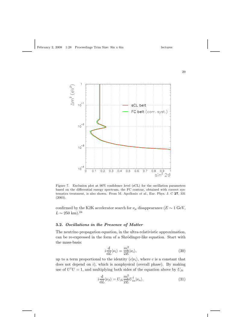
measured far away from the reactor site. For example, the CHOOZ experi-
ment in France,23 has measured the flux of electron-type reactor antineutri-
nos a little over one kilometer from the source. They have established that
the observed flux agrees with the predicted one, and are able to set bounds
on neutrino oscillation parameters, as depicted in Fig. 7. The shape of the
exclusion curve is easy to understand. For ∆m2L/4E ≫ 1, the oscillatory
effects average out (remember that the reactor spectrum is continuos, and
that the detector has a finite energy resolution) and Pee ≃ 1 − 1/2 sin2 2θ.
The CHOOZ result, which can be translated into, roughly, Pee > 0.95,
bounds sin2 2θ . 0.1. On the other hand, in the limit ∆m2L/4E ≪ 1,
Pee ≃ 1 − sin2 2θ(∆m2)2(170)2 which leads to
(
∆m2)2
sin2 2θ . 10−6. (29)
For many more details, please see Ref. 23.
The final example is related to the atmospheric neutrino data. It is
fit very well by νµ ↔ ντ oscillations with ∆m2 ∼ 2 × 10⁻³ eV2 (such
that Losc ∼ 1000 km for 1 GeV neutrinos) and sin2 2θ ∼ 1. For more
details, see one of the homework problems in the appendix. The neutrino
oscillation interpretation of the atmospheric data has, more recently, been
February 2, 2008 1:28 Proceedings Trim Size: 9in x 6in lectures
29
Figure 7. Exclusion plot at 90% confidence level (sCL) for the oscillation parametersbased on the differential energy spectrum; the FC contour, obtained with correct sys-tematics treatment, is also shown. From M. Apollonio et al., Eur. Phys. J. C 27, 331(2003).
confirmed by the K2K accelerator search for νµ disappearance (E ∼ 1 GeV,
L ∼ 250 km).24
3.2. Oscillations in the Presence of Matter
The neutrino propagation equation, in the ultra-relativistic approximation,
can be re-expressed in the form of a Shrodinger-like equation. Start with
the mass-basis:
id
dL|νi〉 =
m2i
2E|νi〉, (30)
up to a term proportional to the identity (c|νi〉, where c is a constant that
does not depend on i), which is nonphysical (overall phase). By making
use of U †U = 1, and multiplying both sides of the equation above by Uβi
id
dL|νβ〉 = Uβi
m2i
2EU †
iα|να〉. (31)

February 2, 2008 1:28 Proceedings Trim Size: 9in x 6in lectures
30
In the 2 × 2 case,
id
dL
(
|νe〉|νµ〉
)
=∆m2
2E
(
sin2 θ cos θ sin θ
cos θ sin θ cos2 θ
)(
|νe〉|νµ〉
)
, (32)
up to additional terms proportional to the 2 × 2 identity matrix. Eq. (32)
describes the propagation of flavor eigenstates, which contains, in general,
non-diagonal terms and, hence, mixing.
Let us re-examine the Fermi Lagragian, concentrating on the electron-
type neutrinos and their interaction with electrons. After a Fiertz rear-
rangement of the charged-current terms, the Lagrangian is
L ⊃ νeLi∂µγµνeL − 2√
2GF (νeLγµνeL) (eLγµeL) + . . . . (33)
Given the Lagrangian above, we wish to compute the equation of motion
for one electron neutrino state in the presence of a non-relativistic electron
background. In this case, we need to compute
〈eLγµeL〉 = δµ0Ne
2(34)
where Ne ≡ e†e is the average electron number density (which is at rest,
hence the δµ0 part), and the factor of 1/2 comes from the fact that half
of the electron number density is right-handed, while the other half is left-
handed. The neutrinos only see the left-handed half.
Ignoring mass-terms for the time being, the Dirac equation for a one
neutrino state inside a cold electron “gas” is
(i∂µγµ −√
2GF Neγ0)|νe〉 = 0. (35)
Note that Eq. (35) is not Lorentz invariant. Its solutions are still plane-wave
like and, in the ultrarelativistic limit and in the limit that√
2GF Ne ≪ E,
the neutrino dispersion relation is
E ≃ |~p| ±√
2GF Ne, (36)
where the plus sign applies to the positive energy solutions (neutrinos)
and the minus one to the negative energy ones (antineutrinos). The modi-
fied dispersion relation of neutrinos propagating in matter is similar to the
modified dispersion relation of photons propagating inside matter (index of
refraction).√2GF Ne is referred to as the matter potential, because it looks like
a “potential energy” term for the neutrino (using a classical mechanics
analogy, E = T + V ).

February 2, 2008 1:28 Proceedings Trim Size: 9in x 6in lectures
31
It is easy to see how the effects of matter will change Eq. (32):
id
dL
(
|νe〉|νµ〉
)
=
[
∆m2
2E
(
sin2 θ cos θ sin θ
cos θ sin θ cos2 θ
)
+
(
A 0
0 0
)](
|νe〉|νµ〉
)
, (37)
where A = ±√
2GF Ne (+ for neutrinos, − for antineutrinos). A simi-
lar effect also comes from neutral current interactions. These, however,
are common to all (active) neutrino species, and translate into a term in
Eq. (37) proportional to the identity matrix.
Eq. (37) is not easy to solve in general. A is proportional to the electron
number density along the path of the neutrino, which can be a complicated
function of L. Eq. (37) can be thought of as a two-level non-relativistc
quantum mechanical system in the presence of an external potential which
can be “time” dependent.
Under several conditions, however, Eq. (37) can be solved exactly, and
I’ll discuss two of the most useful ones. The first obvious approximation
is to assume that A is a constant. This is a very good approximation for
neutrinos propagating through matter inside the Earth, with the exception
of neutrinos that traverse different “Earth layers” (the crust, the mantle,
the outer core, the inner core).
Rewrite Eq. (37) as
id
dL
(
|νe〉|νµ〉
)
=
(
A ∆/2 sin 2θ
∆/2 sin 2θ ∆cos 2θ
)(
|νe〉|νµ〉
)
, (38)
where ∆ ≡ ∆m2/2E. By comparing Eq. (38) to Eq. (32), it is easy to guess
that (cf. Eq. (27))
Peµ = sin2 2θM sin2
(
∆ML
2
)
, (39)
where θM is some effective matter mixing angle characterisitic of the eigen-
vectors of the Hamiltonian in Eq. (38), while ∆M is the difference between
the eigenvalues of the Hamiltonian in Eq. (38). ∆M is also proportional to
the effective inverse oscillation length in matter. Some trivial linear algebra
reveals
∆M =
√
(A − ∆cos 2θ)2
+ ∆2 sin2 2θ, (40)
∆M sin 2θM = ∆sin 2θ, (41)
∆M cos 2θM = A − ∆cos 2θ. (42)
The presence of matter affects neutrino and antineutrino oscillation dif-
ferently. This effective “CPT-violation” is expected, given that we are
February 2, 2008 1:28 Proceedings Trim Size: 9in x 6in lectures
32
assuming that the neutrinos are propagating in a background of electrons.
The CPT-theorem relates the propagation of neutrinos in an electron back-
ground to the propagation of antineutrinos in a positron background.
Furthermore, the presence of matter allows one to explore the neutrino
mass and mixing landscape “more.” It is instructive to ask what is the
“physical parameter” space of two-flavor neutrino oscillations, i.e., what
are the values of θ and ∆m2 that span all the distinct physical circum-
stances? Here, I’ll choose m22 ≥ m2
1 (one can view this as the definition
of ν1 and ν2 as, respectively, the lighter and the heavier neutrino), such
that ∆m2 ∈ [0,∞}. Under these circumstances, θ = 0 corresponds to
|νe〉 = |ν1〉 (the lighter state), while θ = π/2 corresponds to |νe〉 = |ν2〉 (the
heavier state). Given that oscillation experiments are not sensitive to the
relative phase between the |ν1〉 and |ν2〉 components of |νe〉,n θ ∈ [0, π/2]
describes all physically distinguishable circumstances. Eq. (27), however, is
invariant under θ ↔ π/2− θ, such that it cannot tell whether the |νe〉 state
is “mostly light” (cos2 θ > sin2 θ, the “light-side”25) or “mostly heavy”
(cos2 θ < sin2 θ, the “dark-side”25).
Oscillations in matter, however, do not suffer from the same degener-
acy problem. Since Eq. (40) depends on cos 2θ, oscillations in matter are
sensitive to the entire two-flavor oscillation parameter space. Fig. 8 depicts
Peµ in vacuum and in matter, assuming that the sign of A agrees or dis-
agrees with the sign of cos 2θ. It is clear that when the two signs agree
(disagree), there is an enhancement (supression) of the transition ampli-
tude, sin2 2θM > (<) sin2 2θ. Optimal enhancement can be obtained when
A = ∆cos 2θ, the so-called resonant condition, in which case sin2 2θM = 1.
It is also clear that the oscillation length increases (decreases) with respect
to the vacuum one in the case of a matter enhancement (suppression). An-
other interesting feature is the fact that, for small L, matter effects “don’t
matter.” This is very easy to see by plugging Eq. (41) into Eq. (39) in the
limit ∆ML, ∆L ≪ 1.
3.2.1. Varying Electron Number Density — The MSW Effect
It is curious that in order to understand the oldest neutrino puzzle, one
is required to use more advanced “technology” than the one developed
above.26 Solar neutrinos are created deep inside the Sun where the matter
density is very high and propagate outward until they eventually meet
nCheck this (or see, for example, Ref. 25)!

February 2, 2008 1:28 Proceedings Trim Size: 9in x 6in lectures
33
L(a.u.)
P eµ =
1-P
ee
sign(A)=sign(cos2θ)
A=0 (vacuum)
sign(A)=-sign(cos2θ)
Figure 8. Peµ as a function of L for fixed values of E, ∆m2, A, and sin2 2θ in vacuumand in matter, assuming sign(A) =sign(cos 2θ) and sign(A) = −sign(cos 2θ).
“empty space.” Along the way, the electron number density varies, to a
reasonably good approximation, exponentially.27
In general, there is no exact solution to the propagation of neutrinos in
matter of varying density. However, if certain approximations apply, a nice
qualitative understanding can be obtained.28 This is, fortunately, the case
for solar neutrinos and neutrinos from other astrophysical sources.
First, consider the “Hamiltonian” of Eq. (37), which I reproduce again
below[
∆
(
sin2 θ cos θ sin θ
cos θ sin θ cos2 θ
)
+ A
(
1 0
0 0
)]
, (43)
and compute its eigenvalues as a function of A (for fixed ∆ and θ). These
are depicted in Fig. 9 in the case cos 2θ > 0.
Assume that one starts at very large, positive, values of A (say, inside the
Sun) such that |νe〉 ≃ |ν2M 〉, the heavier Hamiltonian eigenstate associated
to this value of A (this is easy to see from Eq. (43), in the limit A ≫ ∆). Let
us further assume that A decreases “slowly” as a function of L, such that
the system evolves adiabatically. In this case, the initial |νe〉 will track the
heavy “instantaneous Hamiltionian eigenstate,” such that, when A reaches
zero (say, at the “end” of the Sun), the original |νe〉 is now a |ν2〉 state. In
summary
|νe〉 = |ν2M 〉 at the core → |ν2〉 in vacuum, (44)
PEarthee = |〈νe|ν2〉|2 = sin2 θ. (45)
Note that Pee ≃ sin2 θ applies in a wide range of energies and baselines, as
long as the approximations mentioned above apply — ideal to explain the

February 2, 2008 1:28 Proceedings Trim Size: 9in x 6in lectures
34
A(a.u.)
λ(a.u.)
Figure 9. Eigenstates λ of the Hamiltonian Eq. (43) as a function of A, for fixed ∆ andθ, modulo a constant term, common to both eigenstates.
energy independent suppression of the 8B solar neutrino flux! Furthermore,
sin2 θ ∈ [0, 1], which means that large average suppressions of the neutrino
flux are allowed if sin2 θ ≪ 1. This is to be compared with averaged out
vacuum oscillations P vacee = 1 − 1/2 sin2 2θ > 1/2.
One can expand on the result above by loosening some of the assump-
tions. For example, assume that a |νe〉 state is produced in the Sun’s core
as an incoherent mixture of |ν1M 〉 and |ν2M 〉.o Furthermore, introduce an
adiabaticity parameter Pc, which measures the probability that a |νiM 〉matter Hamiltonian state will not exit the Sun as a |νi〉 mass-eigenstate.
Hence
|νe〉 → |ν1M 〉, with probability cos2 θM , (46)
→ |ν2M 〉, with probability sin2 θM , (47)
where θM is the matter angle at the neutrino production point. Further-
oNumerically, this is an excellent approximation, due to the fact that the neutrino pro-duction region inside the Sun is “large,” while the matter oscillation length inside of theSun is “small.”

February 2, 2008 1:28 Proceedings Trim Size: 9in x 6in lectures
35
more,
|ν1M 〉 → |ν1〉, with probability (1 − Pc), (48)
→ |ν2〉, with probability Pc, (49)
|ν2M 〉 → |ν1〉 with probability Pc, (50)
→ |ν2〉 with probability (1 − Pc). (51)
Finally, since P1e = cos2 θ and P2e = sin2 θ, one can simply read off
P Sunee = cos2 θM
[
(1 − Pc) cos2 θ + Pc sin2 θ]
+ sin2 θM
[
Pc cos2 θ + (1 − Pc) sin2 θ]
. (52)
For an exponential electron number density Ne = Ne0e−L/r0, Pc, also re-
ferred to as the crossing probability, is exactly calculable29
Pc =e−γ sin2 θ − e−γ
1 − e−γ, γ = 2πr0∆. (53)
Note that for γ ≫ 1, Pc → 0 as expected, since γ ≫ 1 implies 1/r0 ≪ ∆,
i.e., the natural frequency of the system is much larger than the rate of
change of the potential, which is the adiabatic condition.
The best application of Eq. (52) is in solving the solar neutrino puzzle.
In particular, for Pc = 0, the qualitative description of Pee is depicted in
Fig. 10. This particular shape is ideal to fit the solar data as long as one
requires sin2 θ ∼ 0.3 and ∆m2 ∼ 10−5 eV2 to 10−4 eV2.
The solar neutrino puzzle was ultimately resolved by the KamLAND re-
actor antineutrino experiment. For ∆m2 values in the preferred solar range,
reactor antineutrinos, with typical energies in the 1–10 MeV range, have an
oscillation length Losc . 2 × 10⁵ m. Hence, if one could measure the reac-
tor antineutrino flux some 100 km away from a nuclear reactor, one should
observe an order one suppression (because the solar data implies a large
mixing angle) of the antineutrino flux. The catch is that the expected flux
from a nuclear reactor 100 km away is tiny (remember that Φ ∝ L−2 in the
universe we live in, with 3+1 large spacetime dimensions), which requires a
very big detector or a really powerful nuclear power plant. The KamLAND
collaboration addressed this problem by building a very large liquid scin-
tillator detector (around 1 kton) and placing it around 100 km away from
several nuclear reactors in Japan. It is a very impressive achievement of our
understanding of neutrino and solar physics that the results obtained by
KamLAND regarding the neutrino oscillation parameters agree perfectly
with the results of the solar experiments. This agreement in depicted in
Fig. 11.

February 2, 2008 1:28 Proceedings Trim Size: 9in x 6in lectures
36
Vacuum - Mattertransition
cos4θ13(1- sin22θ12) 1 2
|
cos4θ13sin2θ12
β=23/2GFcos2θ13neEν
∆m21 2
P
E0.0
0.2
0.4
0.6
0.8
1.0
Figure 10. Electron neutrino survival probability, Pee, as a function of neutrino en-ergy for the (daytime) LMA oscillation solution. For small values of the parameter β,the vacuum (kinematic) oscillation effects are dominant. For values of β greater thanunity, the MSW (matter) oscillations are most important. In order to properly fit thesolar neutrino data, the transition between vacuum and matter oscillations should occursomewhere in the region of 2 MeV. In the case of two flavor oscillations, set θ13 = 0,and θ12 = θ. From http://www.sns.ias.edu/∼jnb and J.N. Bahcall and C. Pena-Garay,JHEP 0311, 004 (2003).
4. Solving the Neutrino Puzzles
In order to fit solar, atmospheric, reactor and accelerator neutrino data
(except for the LSND anomaly, cf. Sec. 5), it is clear that two-flavor oscil-
lations do not suffice. The reason for this is obvious: among other things,
solar/KamLAND and atmospheric/K2K data point to very different values
of the mass-squared difference and the mixing angle. Of course, the situ-
ation is naively remedied once one remembers that we are aware of three
neutrinos — not two.
For three neutrino flavors, the MNS matrix is defined as
νe
νµ
ντ
=
Ue1 Ue2 Ue3
Uµ1 Uµ2 Uµ3
Uτ1 Ueτ2 Uτ3
ν1
ν2
ν3
, (54)

February 2, 2008 1:28 Proceedings Trim Size: 9in x 6in lectures
37
)2 (
eV2
m∆
-510
-410
θ 2tan
-110 1 10
KamLAND
95% C.L.
99% C.L.
99.73% C.L.
KamLAND best fit
Solar
95% C.L.
99% C.L.
99.73% C.L.
solar best fit
θ 2tan
0.2 0.3 0.4 0.5 0.6 0.7 0.8
)2 (
eV2
m∆KamLAND+Solar fluxes
95% C.L.
99% C.L.
99.73% C.L.
global best fit-510×4
-510×6
-510×8
-410×1
-410×1.2
Figure 11. LEFT – Neutrino oscillation parameter allowed region from KamLANDanti-neutrino data (shaded regions) and solar neutrino experiments (lines). RIGHT –Result of a combined two-neutrino oscillation analysis of KamLAND and the observedsolar neutrino fluxes. The fit gives ∆m2 = 7.9+0.6
−0.5 × 10⁻⁵ eV2 and tan2 θ = 0.40+0.10−0.07
including the allowed one sigma parameter range. From T. Araki et al. [KamLANDCollaboration], hep-ex/0406035.
and its elements are, of course, not all independent. It is customary6 to
parameterize U in Eq. (54) with three mixing angles θ12, θ13, θ23 and three
complex phases, δ, ξ, η, defined by
|Ue2|2|Ue1|2
≡ tan2 θ12;|Uµ3|2|Uτ3|2
≡ tan2 θ23; Ue3 ≡ sin θ13e−iδ, (55)
with the exception of ξ and η, the so-called Majorana CP-odd phases.
These are only physical if the neutrinos are Majorana fermions, and have,
unfortunately, virtually no effect in flavor-changing phenomena.p We have
no idea what their values are or even whether they are physical observables!
In order to proceed unambiguously, it is necessary to define the neutrino
mass eigenstates, i.e., to “order” the neutrino masses. This is most often
done in the following way: m22 > m2
1 and ∆m212 < |∆m2
13|. In this case,
there are three mass-related observables: ∆m212 (positive definite), |∆m2
13|,and the sign of ∆m2
13. A positive sign for ∆m213 implies m2
3 > m22 — a
so-called normal mass-hierarchy — while a negative sign for ∆m213 implies
m23 < m2
1 — a so-called inverted mass-hierarchy. The two distinct neutrino
mass-hierarchies are depicted in Fig. 12. Finally, the data tell us that the
pfor a more detailed discussion of Majorana phases and their physical effects, see, forexample, Ref. 31

February 2, 2008 1:28 Proceedings Trim Size: 9in x 6in lectures
38
ratio ∆m212/|∆m2
13| . 1/30 is small. We will take full advantage of that in
what follows.
(∆m2)sol
(∆m2)sol
(∆m2)atm
(∆m2)atm
νe
νµ
ντ
(m1)2
(m2)2
(m3)2
(m1)2
(m2)2
(m3)2
normal hierarchy inverted hierarchy
Figure 12. Cartoon of the two distinct neutrino-mass hierarchies that fit all of thecurrent neutrino data, for fixed values of all mixing angles and mass-squared differences.The color coding (shading) indices the fraction |Uαi|2 of each distinct flavor να, α =e, µ, τ contained in each mass eigenstate νi, i = 1, 2, 3. For example, |Ue2|2 is equal tothe fraction of the (m2)2 “bar” that is painted red (shading labeled as ‘νe’).
In vacuum, the oscillation probabilities can be written as
Pαβ = δαβ + Asolαβ sin2
(
∆m212L
4E
)
+ Aatmαβ sin2
(
∆m213L
4E
)
+
+F intαβ (L, ∆m2
12, ∆m213), (56)
where Aαβ are the “solar” and “atmospheric” amplitudes, functions of Uαi,
while Fαβ are “interference terms.”q
The survival probability of atmospheric muon-type neutrinos is given
by
P atmµµ ≃ 1 − 4|Uµ3|2
(
1 − |Uµ3|2)
sin2
(
∆m213L
4E
)
, (57)
qI’ll leave as an exercise to show that this is the case, and to figure out what theexpressions for the A’s and F ’s are.

February 2, 2008 1:28 Proceedings Trim Size: 9in x 6in lectures
39
ignoring effects from the “solar” oscillation length, which will turn out to be
much longer than the the Earth’s diameter for typical atmospheric neutrino
energies. For the same reason, the survival probability of reactor electron-
type antineutrinos at the CHOOZ experiment (L ∼ 1 km) can be written
as
PCHOOZee ≃ 1 − 4|Ue3|2
(
1 − |Ue3|2)
sin2
(
∆m213L
4E
)
. (58)
Eq. (57) and Eq. (58) are effective two flavor oscillation expressions, and
the data require (i) ∆m213 ≃ 2 × 10⁻³ eV2, (ii) |Uµ3|2 ≃ 0.5, and (iii)
|Ue3|2 ≡ sin2 θ13 . 0.05. Unitarity of U combined with (ii) and (iii) lead to
|Uτ3|2 ≃ 0.5, such that tan2 θ23 ≃ 1.
The survival probability of electron-type neutrinos from the Sun and
antineutrinos from reactors at KamLAND is given by
Pee ≃ cos4 θ13P2νee (∆m2
12, sin2 θ12) + sin4 θ13, (59)
where P 2νee is the appropriate two-flavor neutrino oscillation equation with
∆m2 = ∆m212, sin2 θ = sin2 θ12, and a modified matter potential A →
A cos2 θ13. The reasons behind the validity of Eq. (59) are (i) “atmospheric”
effects average out given that the associated oscillation lengths are much
smaller than the baselines of the KamLAND experiment and (ii) the matter
potential in the Sun’s core is significantly smaller than |∆m213|/(2E) for
solar neutrino energies.
Again, Eq. (59) is almost an effective two-flavor oscillation expression
(especially because θ13 is known to be small), and the data point to ∆m212 ∼
10−4 eV2 and sin2 θ12 ∼ 0.3.
Detailed combined analyses of all neutrino data are consistent, at the
three sigma confidence level, with32
• sin2 θ12 = 0.30 ± 0.08, mostly from solar data;
• sin2 θ23 = 0.50 ± 0.18, mostly from atmospheric neutrino data;
• sin2 θ13 ≤ 0047, mostly from atmospheric and CHOOZ data;
• ∆m212 = 8.1 ± 1.0 eV2, mostly from KamLAND data;
• |∆m213| = 2.2 ± 1.1 eV2, mostly from atmospheric neutrino data.
These results are summarized in Fig. 13.r As one can clearly see, in the
span of less than a decade we have “evolved” from not being sure whether
neutrinos had mass to “precisely” measuring the neutrino mass-squared
rIn the figure, ∆m2ij is defined by m2
i −m2j , as opposed to the one I adopt here, m2
j −m2i .
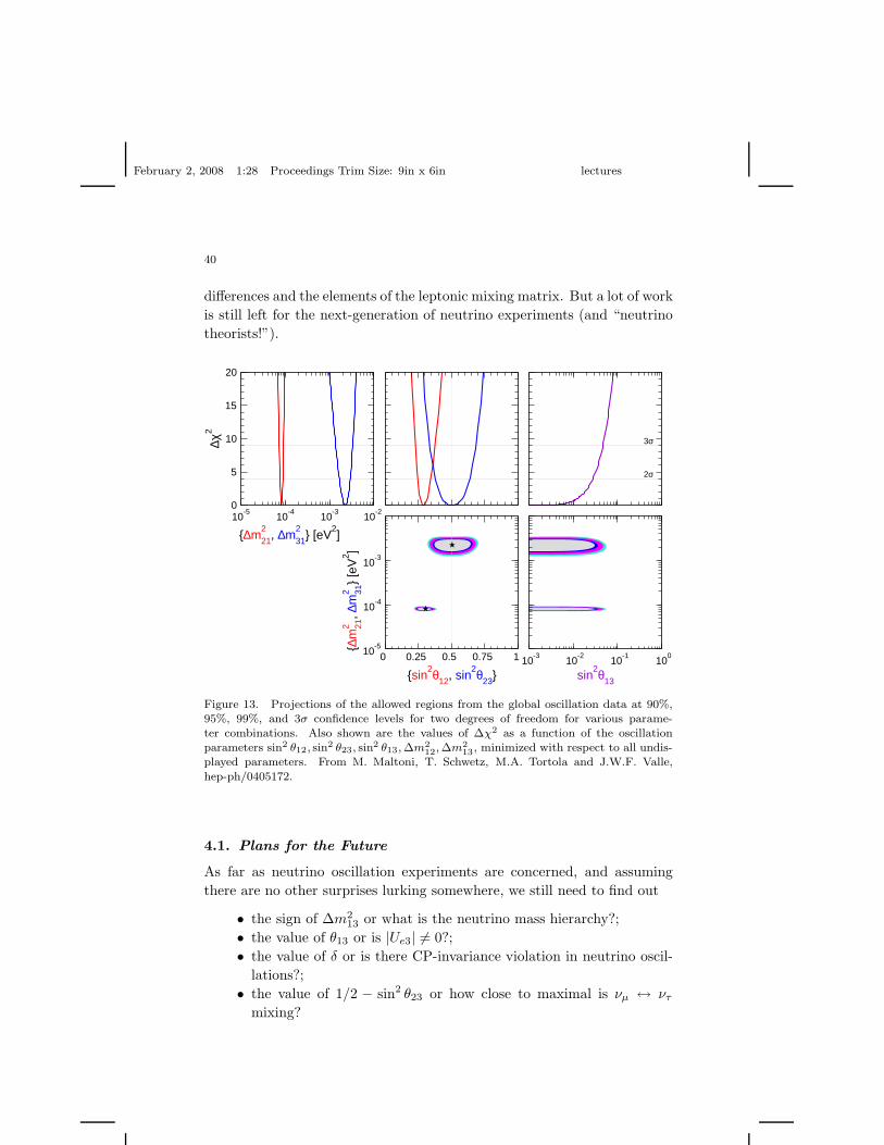
February 2, 2008 1:28 Proceedings Trim Size: 9in x 6in lectures
40
differences and the elements of the leptonic mixing matrix. But a lot of work
is still left for the next-generation of neutrino experiments (and “neutrino
theorists!”).
10-5
10-4
10-3
10-2
{∆m221, ∆m
231} [eV
2]
0
5
10
15
20
∆χ2
3σ
2σ
★
★
0 0.25 0.5 0.75 1
{sin2θ12, sin
2θ23}
10-5
10-4
10-3
{∆m
2 21, ∆
m2 31
} [e
V2 ]
10-3
10-2
10-1
100
sin2θ13
Figure 13. Projections of the allowed regions from the global oscillation data at 90%,95%, 99%, and 3σ confidence levels for two degrees of freedom for various parame-ter combinations. Also shown are the values of ∆χ2 as a function of the oscillationparameters sin2 θ12, sin2 θ23, sin2 θ13, ∆m2
12,∆m213, minimized with respect to all undis-
played parameters. From M. Maltoni, T. Schwetz, M.A. Tortola and J.W.F. Valle,
hep-ph/0405172.
4.1. Plans for the Future
As far as neutrino oscillation experiments are concerned, and assuming
there are no other surprises lurking somewhere, we still need to find out
• the sign of ∆m213 or what is the neutrino mass hierarchy?;
• the value of θ13 or is |Ue3| 6= 0?;
• the value of δ or is there CP-invariance violation in neutrino oscil-
lations?;
• the value of 1/2 − sin2 θ23 or how close to maximal is νµ ↔ ντ
mixing?

February 2, 2008 1:28 Proceedings Trim Size: 9in x 6in lectures
41
Furthermore, we need to know several of the already-measured oscillation
parameters more precisely in order to start filling in the gaps. Current,
near-future, and far-future experiments are being built/planned/considered
in order to fully piece together the neutrino flavor-change phenomenon.
There are “on-going” long baseline experiments. All of these consist of
a muon-neutrino beam, just like the one used to discover the muon-type
neutrino, aimed at a detector some hundreds of kilometers away. These
include
• The K2K experiment (“KEK to Kamionka”), already alluded to
and currently taking data in Japan. K2K studies the disappearance
of muon-type neutrinos in the “atmospheric frequency.” K2K data
agree with Super-Kamiokande atmospheric neutrino data, and the
collaboration has recently reported a hint of an “oscillatory sup-
pression” of the νµ-flux;24
• The MINOS experiment (“Main Injector Neutrino Oscillation
Search”), is being built at Fermilab and should start data tak-
ing in the end of 2004.33 It is similar to the K2K experiment,
with a longer baseline (L = 732 km) and higher neutrino energies
(E ∼ 1 − 10 GeV). Minos has the ability to see a more pronounced
oscillatory behavior of the muon spectrum at the far detector, and
will be able to measure ∆m213 more precisely than K2K. It is also
more sensitive to νµ → νe appearance driven by a nonzero |Ue3|2than CHOOZ was sensitive to νe disappearance (by about a factor
of two).
• The CNGS (“CERN Neutrinos to Gran Sasso”) project is being con-
structed at CERN, and aims at starting data taking in a few years.34
Its baseline is similar to the MINOS one, but the typical neutrino
energies are much higher (tens of GeV). Among other things, it is
sensitive to tau-appearance driven by the expected “atmospheric”
νµ ↔ ντ oscillations.
Near-future oscillation experiments are either under construction or
their proposals are (in most cases) under review.s I’ll highlight two classes
of experiments:
• Long baseline experiments optimized to study νµ → νe transitions
sA recent study of the future of neutrino physics has recently become available.35 Itdescribes future experiments in much more detail, and contain a large amount of infor-mation.

February 2, 2008 1:28 Proceedings Trim Size: 9in x 6in lectures
42
governed by the atmospheric mass-squared difference. In this case
Peµ ∝ |Umattere3 |2 cos2 θ23 sin2
(
∆matter13 L
2
)
+ . . . (60)
where the ‘matter’ superscripts indicate that matter effects may be
sizeable, and the ellipsis indicate sub-leading effects due to “solar”
oscillations.
These setups are not only sensitive to |Ue3|2, but are also sensi-
tive to the sign of ∆m213, as long as the matter effects are significant.
Furthermore, they are also sensitive to effects of the CP-odd phase
δ.
• Next-generation reactor experiments, with baselines around one
kilometer. Here the oscillation probability is given by Eq. (58),
and the goal is to improve on the sensitivity of the CHOOZ ex-
periment by an order of magnitude. This is hoped to be achieved
by optimizing the reactor–detector distance, and adding a near-
detector, capable of measuring the reactor antineutrino flux and
reducing systematic errors significantly.36 Complementary to long-
baseline νµ → νe studies, these setups are only sensitive to |Ue3|2.Hence, they can obtain a very “clean” measurement of |Ue3|2, but
do not have the ability to determine the mass-hierarchy or whether
CP-invariance is violated in the neutrino oscillations.
Further in the future, the neutrino community is contemplating building
completely new neutrino facilities, capable of providing different, precisely
calculable neutrino beams. Among them are
• Neutrino Factories, or muon storage rings. The idea is to accelerate
and “store” muons in a ring-like structure.37 Natural muon decay
produces an intense, very well known beam of muon-type neutrinos
and electron-type antineutrinos (or vice-versa, depending on the
muon-charge). Note that neutrino factories offer a very intense,
high energy electron-type neutrino beam, something we have not
been able to work with so far! This allows one to study νe → νµ
transitions (as opposed to νµ → νe). νe → νµ not only serves as
a new channel to probe neutrino flavor change, but it is often the
case that high-energy muons are easier to study in typical neutrino
detectors than electrons.
• More recently, the community has been considering a different op-
tion for generating a high energy electron-type neutrino beam —

February 2, 2008 1:28 Proceedings Trim Size: 9in x 6in lectures
43
β−beams.38 These consist of accelerating to large γ-factors and
storing β− and β+ decaying nuclei (say, 6He→6Li+e− + νe and18Ne→18F+e+ + νe) and using them as sources of electron-type an-
tineutrinos or neutrinos, respectively.
Needless to say, there are many physics and technology (and financial)
issues that need to be resolved before either neutrino factories or beta-
beam facilities can be built. They are, nonetheless, the subject of serious
research and development activity and are viewed as the most powerful
tools to study neutrinos in particular, and lepton physics in general. They
may ultimately be required in order for us to obtain a deeper and more
satisfying understanding of neutrinos.
5. Unsolved Puzzle — the LSND Anomaly
The LSND experiment39 measured the neutrino flux produced by pion de-
cay in flight (π+ → µ+νµ) and antimuon decay at rest (µ+ → e+νeνµ). It
observed a small electron-type antineutrino flux some 30 meters away from
the production region.39 The originally absent νe-flux can be interpret as
evidence that νµ is transforming into νe with Pµe of the order a fraction
of a percent. The data also contain a weak hint of a νe excess, which is
both consistent with the νµ → νe hypothesis and consistent with zero. If
interpreted in terms of two-flavor neutrino oscillations, the LSND anomaly,
combined with constraints imposed by several other experiments, points to
a mass-squared difference ∆m2LSND ∼ 0.1 − 10 eV2, as depicted in Fig. 14.
The LSND result will be confirmed or refuted by the on-going Mini-
BooNE experiment, perhaps as early as the end of Summer 2005.40 Mini-
BooNE consists of a standard νµ-beam experiment (from π+ decay), with
neutrino energies in the sub-GeV to GeV range and a baseline of around
500 m. Its beam (neutrino versus antineutrino) and systematics are quite
distinct from the LSND setup.
It is easy to understand why the LSND anomaly does not “fit” in the
three flavor mixing scheme described in the previous section. With three
neutrinos, one can define only two independent mass-squared differences,
and these are completely determined by the solar, atmospheric, reactor,
and accelerator data. As discussed earlier, both mass-squared differences
are much smaller than ∆m2LSND. Given that the LSND results are yet to be
confirmed by another experiment — indeed, the Karmen 2 experiment,41
using a similar setup but with a shorter baseline (L = 18 m), could have
confirmed the LSND anomaly but did not observe any excesses, ruling out
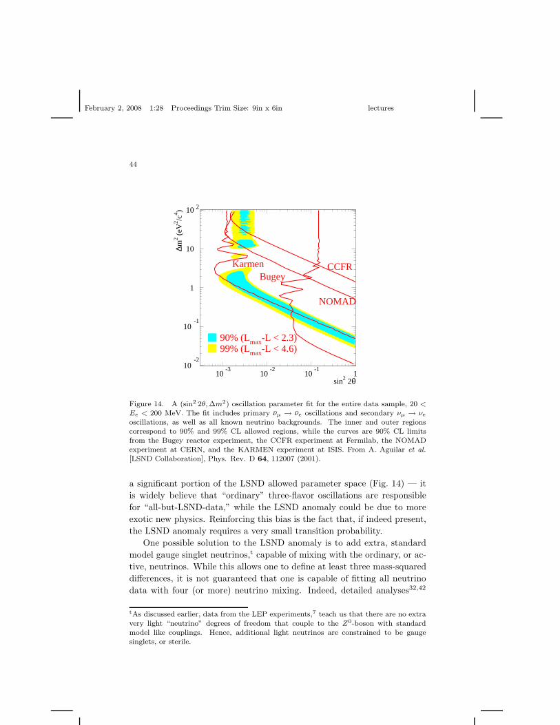
February 2, 2008 1:28 Proceedings Trim Size: 9in x 6in lectures
44
10-2
10-1
1
10
10 2
10-3
10-2
10-1
1sin2 2θ
∆m2 (
eV2 /c
4 )
BugeyKarmen
NOMAD
CCFR
90% (Lmax-L < 2.3)99% (Lmax-L < 4.6)
Figure 14. A (sin2 2θ, ∆m2) oscillation parameter fit for the entire data sample, 20 <
Ee < 200 MeV. The fit includes primary νµ → νe oscillations and secondary νµ → νe
oscillations, as well as all known neutrino backgrounds. The inner and outer regionscorrespond to 90% and 99% CL allowed regions, while the curves are 90% CL limitsfrom the Bugey reactor experiment, the CCFR experiment at Fermilab, the NOMADexperiment at CERN, and the KARMEN experiment at ISIS. From A. Aguilar et al.
[LSND Collaboration], Phys. Rev. D 64, 112007 (2001).
a significant portion of the LSND allowed parameter space (Fig. 14) — it
is widely believe that “ordinary” three-flavor oscillations are responsible
for “all-but-LSND-data,” while the LSND anomaly could be due to more
exotic new physics. Reinforcing this bias is the fact that, if indeed present,
the LSND anomaly requires a very small transition probability.
One possible solution to the LSND anomaly is to add extra, standard
model gauge singlet neutrinos,t capable of mixing with the ordinary, or ac-
tive, neutrinos. While this allows one to define at least three mass-squared
differences, it is not guaranteed that one is capable of fitting all neutrino
data with four (or more) neutrino mixing. Indeed, detailed analyses32,42
tAs discussed earlier, data from the LEP experiments,7 teach us that there are no extra
very light “neutrino” degrees of freedom that couple to the Z0-boson with standardmodel like couplings. Hence, additional light neutrinos are constrained to be gaugesinglets, or sterile.

February 2, 2008 1:28 Proceedings Trim Size: 9in x 6in lectures
45
suggest that four neutrino mixing schemes are either very poor or at best
mediocre fits to all neutrino data.
The reason for this can be qualitatively understood in the following
way. There are two general neutrino mass-patterns capable of describing
one large and two small mass-squared differences. These are referred to as
the “2+2” and “3+1” scheme, and are depicted in Fig. 15.
(∆m2)sol (∆m2)sol
(∆m2)atm
(∆m2)atm
(∆m2)LSND
(∆m2)LSND
νe
νµ
ντ
νs
2+2 3+1
Figure 15. Two possible mass-patterns potentially capable of addressing all neutrinodata, including those from LSND. The one on the left (right) is characteristic of a “2+2”(“3+1”) mass-scheme.
The 2+2 schemes are disfavored for the following reason. Short baseline
neutrino data constrain |Uµ1|, |Uµ2|, |Ue3|, |Ue4| to be small.u If all of these
are set to zero, atmospheric oscillations are driven by |νµ〉 ↔ cos ζ|ντ 〉 +
sin ζ|νs〉 mixing, where νs is a sterile neutrino and ζ is a mixing angle
that characterizes the sterile component of the atmospheric neutrino “pair”
of the muon-type neutrino. By unitarity, solar oscillations are driven by
|νe〉 ↔ − sin ζ|ντ 〉 + cos ζ|νs〉 mixing.
Both solar and atmospheric data constrain ζ. Atmospheric neutrino
data are sensitive to a sterile component via Earth matter effects, and due
uHere, |∆m212| ≡ ∆m2
sol, |∆m2
34| ≡ ∆m2atm.

February 2, 2008 1:28 Proceedings Trim Size: 9in x 6in lectures
46
to the fact that tau-type neutrinos also interact with the detector. So-
lar data are sensitive to a sterile component via matter effects in the Sun
and in the Earth, and also due to the fact that tau-type neutrinos inter-
act via neutral current interactions inside of SNO and Super-Kamiokande.
Both solar and atmospheric data see no evidence for a sterile component.
Hence, atmospheric data set an upper bound for sin2 ζ, while the solar data
require a small cos2 ζ. By combining both data sets, cos2 ζ + sin2 ζ is al-
ready constrained to be less than one,32,42 “ruling out” the 2+2 scheme.
Some attempts have been made at understanding what happens when the
conditions |Uµ1| = |Uµ2| = |Ue3| = |Ue4| = 0 are lifted consistent with
experimental bounds (see, for example, Ref. 43) but one expects that these
sub-leading effects will not lead to a significantly better fit.
The 3+1 schemes fit the atmospheric and solar data just fine, given that
sterile neutrino effects are just a small perturbation to the ordinary three
neutrino fit to all-but-LSND data. They run into some trouble when it
comes to short-baseline searches for νe and νµ disappearance driven by the
LSND frequency (see Fig. 14). LSND νµ ↔ νe oscillations are given byv
Peµ ≃ 4|Ue4|2|Ue4|2 sin2
(
∆m2LSNDL
4E
)
, (61)
while the survival probability of a species α = e, µ, for “short” L, is given
by
Pαα ≃ 1 − 4|Uα4|2(1 − |Uα4|2) sin2
(
∆m2LSNDL
4E
)
. (62)
The absence of electron-type and muon-type neutrino disappearance con-
strains |Ue4|2, |Uµ4|2 to be small, while the LSND data require |Ue4|2×|Uµ4|2to be larger than a fraction of a percent.44 The tension in the current data
is not enough to rule out the 3+1 schemes, but it does lead to a mediocre
fit.32,42
Five neutrino mixing schemes have also been explored (see, for example,
Ref. 45). These look like “3+1+1” schemes (“2+2+1” schemes do not fare
much better than 2+2 schemes) and are designed in a such a way that the
tension between the short-baseline and the LSND data is alleviated. With
five neutrinos, it is possible to fit all the neutrino data properly, but some
worry that the choices for mixing parameters and mass-squared differences
are rather “finely tuned.”
vHere, ∆m2LSND ≃ |∆m2
i4|, ∀i = 1, 2, 3.
February 2, 2008 1:28 Proceedings Trim Size: 9in x 6in lectures
47
More exotic solutions to the LSND anomaly have been proposed, and
none of them seem to fit all data particularly well. Here I list some of them.
The possibility that there are rare lepton-flavor violating µ+ → e+νανe
decays46 could explain the LSND data as long as the branching ratio for
the flavor-violating decay was of order a fraction of a percent. Such decays,
however, should also have been observed by the Karmen experiment, which
disfavored this hypothesis at around the 90% confidence level.47 Recently
available precision data of the Michel electron energy spectrum48 seem to
safely rule out flavor changing muon decays as a solution to the LSND
anomaly.
Postulating that neutrinos and antineutrinos have different masses and
mixing angles49 received a significant amount of attention in the past three
years. The original idea was inspired by the fact that solar data required the
disappearance of electron-type neutrinos, while those from LSND required
the appearance of electron-type antineutrinos. If neutrinos and antineu-
trinos oscillated at different frequencies (different ∆m2), all data could be
rendered compatible. Aside from all sorts of theoretical issues, the orig-
inal CPT-violating setup was ruled out when KamLAND published the
first evidence for antineutrino oscillations at solar frequencies. A second
manifestation of CPT-violating solutions the the LSND data consisted of
postulating that atmospheric oscillations in the antineutrino sector were
driven by ∆m2LSND. This possibility is strongly disfavored (at the three
sigma level) by the atmospheric data.50
Given the fact that none of the solutions to the LSND anomaly proposed
to date seem completely satisfactory, it is fair to say that if MiniBooNE
confirms the observations made by LSND, there is a good chance we have
uncovered a novel physical phenomenon, i.e., we are yet to figure out what
the LSND result is teaching us. This being the case, if the LSND anomaly
is confirmed, all the necessary experimental and theoretical efforts will most
likely concentrate, first, on uncovering the mechanism responsible for the
LSND flavor change. This will likely require (i) detailed analysis of all avail-
able data, (ii) new, compelling ideas, and (iii) a series of other experimental
neutrino efforts, capable of mapping out the LSND/MiniBooNE potential
parameter spaces. We are still not sure what these should be!
6. What Have We Learned?
If one were to summarize in one sentence what we have learned after six
years of remarkable experimental results, this would be it:

February 2, 2008 1:28 Proceedings Trim Size: 9in x 6in lectures
48
Neutrinos have (very, very tiny) masses.
Massive neutrinos constitute the only palpable evidence we have that the
standard model of electroweak, and strong interactions (SM) does not de-
scribe all strong, electromagnetic and weak phenomena.
Fig. 16 depicts the value of the masses of all known fundamental
fermions. Note the logarithmic scale. Fermion masses are very hierar-
chical — it takes over thirteen orders of magnitude to fit them all in one
plot! Quark masses span five orders of magnitude, while charged fermion
masses span over three orders of magnitude. We don’t know why fermion
masses are distributed in this way.
1
2
3
10-5
10-4
10-3
10-2
10-1
1 10 102
103
104
105
106
107
108
109
1010
1011
1012
mass (eV)
gene
ratio
n
t
b
τµ
c
sd
u
e
ν3
ν2
ν1
TeVGeVMeVkeVeVmeV
Figure 16. Masses of all known fundamental fermions. A normal mass-hierarchy hasbeen assumed — m2
ν1< m2
ν2< m2
ν3— together with a rather conservative upper bound
m2νi
< 1 eV ∀i = 1, 2, 3. The light, hatched region indicates the six-orders-of-magnitude“desert” between the largest possible neutrino mass and the electron mass.
It is remarkable that the ratio of the largest possible neutrino mass to
the lightest known charged fermion mass (the electron mass) is at least one
order of magnitude less than the ratio of the electron mass to the top quark
mass. Furthermore, while the electron–top “gap” is populated by all other
charged leptons and quarks, the heaviest-neutrino–electron “gap” seems to
be deserted. We also don’t know why this is the case, but it does seem to
be Nature’s way of saying that there is something special about neutrino
masses. It may be that neutrino masses are qualitatively different from
charged fermion masses.

February 2, 2008 1:28 Proceedings Trim Size: 9in x 6in lectures
49
Before proceeding, I’ll very briefly summarize the SM, and what I mean,
here, by going beyond it (see also Ref. 5). The SM is a Lorentz invariant
quantum field theory, and its renormalizable Lagrangian is uniquely deter-
mined once one specifies its internal symmetries (gauged SU(3)c×SU(2)L×U(1)Y invariance) and particle content (Q, u, d, L, e, the matter fields, plus
H , the Higgs doublet scalar field). The fact that the Lagrangian is renor-
malizable implies that, naively, the SM is valid up to arbitrarily high energy
scales (ignoring gravity, etc). It is easy to check that given the SM as de-
fined above, neutrinos are strictly massless.
There are several ways of modifying the SM and allowing nonzero neu-
trino masses. The amount of experimental information available is, how-
ever, still insufficient to allow a particular candidate “new SM” to be chosen
over another, but there is reason to believe that more information is on the
way in the near (few years) to intermediate (several years) future. Here,
I’ll very briefly present two “minimal paradigms.”
Arguably, the simplest way to “add” neutrino masses to the SM is to
give up on the renormalizability of the Lagrangian. This allows one to add
(an infinite number of) irrelevant operators consistent with the symmetries:
Lnew = LSM − λαβ LαHLβH
2M+ O
(
1
M2
)
. (63)
All fermion fields are understood to be Weyl fermions, such that, for exam-
ple, the charged lepton Yukawa operator is written as LHe, where e is the
(positively) charged-lepton SU(2)L singlet field.
Two facts are remarkable. One is that (LH)2 is the only type of
dimension-five operator allowed by the SM gauge invariance and parti-
cle content.51 The other is that, as long as M is much larger than 〈H〉,the Higgs vacuum expectation value, the only observable consequence of
Eq. (63)w is that neutrinos get a nonzero mass after electroweak symmetry
breaking: mν = λ〈H〉2/M . An extra “bonus” is that neutrino masses are
naturally much smaller than all other fermion masses mf ∝ 〈H〉 by a factor
〈H〉/M .
Another important consequence of Eq. (63) is that lepton number is
not a good symmetry ((LH)2 breaks lepton number by two units). Lepton
number violation is “encoded” in the fact that the neutrinos are Majorana
fermions.
wThis is not necessarily correct. One also has to worry about dimension six operatorsthat lead to baryon number violation and a finite lifetime for the proton.
February 2, 2008 1:28 Proceedings Trim Size: 9in x 6in lectures
50
M can be described, roughly, as the energy scale above which Eq. (63) is
no longer valid. There is very little information regarding the magnitude of
M , but one can set an upper bound for M by assuming that λ ∼ 4π,52 i.e.,
by assuming that the physics replacing Eq. (63) at the scale M is strongly
coupled. In this case
M . 4π〈H〉2mν
∼ 1015 GeV
(
100 meV
mν
)
. (64)
If Eq. (63) is indeed the correct low-energy description of Nature, neutrino
masses represent the first direct evidence that the SM is an effective field
theory, valid up to an energy scale less that 1015 GeV (or so), which is,
in turn, much less than the Planck scale.52,53 It is also impressive that the
upper bound above coincides, qualitatively, with the energy scale where all
three running gauge coupling constants of the SM seem to meet, MGUT ∼1015−16 GeV.
There are several different proposals for the physics that replaces
Eq. (63). The most famous one is the seesaw mechanism,54 described in
detail in Ref. 5.
A completely different option is to assume that neutrinos are, similar to
all charged matter fields, Dirac fermions. In this case, in order to render the
neutrinos massive, it suffices to add extra SM gauge singlet Weyl fermions
Ni (“right-handed neutrinos”), and Yukawa couplings between H , Lα, Ni:
Lnew = LSM − yαiLαHNi + H.c. . (65)
After electroweak symmetry breaking, the neutrino mass matrix is given
by mν = y〈H〉, similar to the up-type and down-type quark mass matri-
ces and the charged lepton mass matrix. The magnitude of the neutrino
masses requires y . 10−12, at least six orders of magnitude smaller than
the electron Yukawa coupling. It is clear that a natural explanation for
the smallness of the neutrino mass is not contained in Eq. (65). On the
positive side, Eq. (65) is renormalizable, meaning that this new SM version
is, naively, valid up to arbitrarily high energy scales.
Modulo a natural explanation for the size of the neutrino mass, one
could try to argue that Eq. (65) is a rather innocuous addition to the SM
Lagrangian. I believe this is not the case. Eq. (65) is not the most general,
renormalizable Lagrangian consistent with the symmetries of the SM. Once
the fields Ni are introduced, the dimension-three Majorana mass operators12M ij
N NiNj should also have been introduced, given the fact that Ni’s are
gauge singlets. One needs, therefore, to modify the symmetry structure

February 2, 2008 1:28 Proceedings Trim Size: 9in x 6in lectures
51
of the SM in order to forbid a Majorana mass term for the right-handed
neutrinos. One simple way of doing this is to add to the SM an internal
global symmetry, e.g. U(1)B−L, where B stands for baryon number, and
L for lepton number.x Note that, in the massless-neutrino SM, U(1)B−L
is an accidental global symmetry, i.e., it arises as a consequence of the
imposed gauge symmetries and the particle content. Among other things,
this means that there was, a priori, no reason to believe that it needed to
be conserved by allowed SM extensions, including SUSY, quantum gravita-
tional effects, etc. If Eq. (65) is indeed the correct description of neutrino
masses, U(1)B−L needs to be “upgraded” to an imposed fundamental global
symmetry, and it is expected to be preserved by, say, quantum gravity, etc.
Several distinct mechanisms for explaining naturally light Dirac neu-
trino masses exist, for example, in the various models with either “large”
or “warped” extra dimensions.55,56,57 This is rather convenient, given that
most realizations of these models have a rather low ultraviolet cutoff, mean-
ing that these models are effective field theories that need to be replaced by
unknown new physics at energy scales well below the Planck mass (more
often, close to the electroweak breaking scale). Therefore, in order to avoid
generic dimension-five operators as in Eq. (63) suppressed by M & 1 TeV
and hence unacceptably large Majorana neutrino masses, one is “required”
to impose U(1)B−L (or something similar) as a fundamental global sym-
metry.y
6.1. The Faith of Lepton Number
Except for the nature of the neutrinos, both neutrino mass paradigms
— Eq. (63) and Eq. (65) — predict one and the same thing: neutrinos
have mass. In order to make significant progress in understanding neu-
trino masses, it is clear that we need to establish, by some means, whether
neutrinos are Dirac or Majorana fermions.
The way to test whether neutrinos are Majorana fermions is to look
for processes that violate lepton number, including forbidden decays like
K+ → π−µ+µ+ and/or scattering processes, like νe + p → e+ + n. It
turns out that if the neutrinos are Majorana fermions, all such processes
xU(1)B−L is not anomalous, meaning it is not broken by non-perturbative quantummechanical effects, unlike U(1)B or U(1)L.yIn all fairness, this is not a unique “feature” of extra-dimensional theories. The MSSM,
for example, runs into similar problems if R-parity is not imposed as a fundamentalsymmetry. This is, of course, a consequence of the fact that U(1)B−L is an accidental
symmetry of the SM.

February 2, 2008 1:28 Proceedings Trim Size: 9in x 6in lectures
52
are expected to occur with nonzero probability. The reason for this is
simple. If neutrinos are Majorana fermions, U(1)L (and U(1)B−L) are
not good symmetries of the SM, and nothing would prevent, say, K+ →π−µ+µ+ from happening. The converse is also true — if there are physical
processes that violate baryon number minus lepton number, then neutrinos
are Majorana fermions.58
If, however, the neutrino masses are the only source of lepton number
violation, lepton number violating effects are, numerically, tiny. This is
easy to see. If the neutrino mass mν is the only parameter that “knows”
about lepton number violation, the amplitude for any lepton-number vio-
lating process should vanish when mν → 0 (when the accidental U(1)B−L
symmetry is restored) such that AL/ ∝(
mν
E
)n, where n is positive and E
is the typical energy scale involved in the process of interest. Because neu-
trino masses are tiny compared to any reasonable value of E, the rate of
lepton number violating processes is expected to be hopelessly small.
Given the current bounds on neutrino masses and mixing, the “only
hope” for probing lepton number violation mediated by Majorana neutrino
masses with enough sensitivity is to look for neutrinoless double-beta decay,
0νββ.59
Two-neutrino double beta decay (2νββ) is a nuclear process through
which a Z-charged nucleus decays “directly” to a Z + 2-charged nucleus:
Z → (Z + 2) + e− + e− + νe + νe. (66)
Such processes have been observed for several nuclei, including 76Ge, 100Mo,130Te, etc. Typical half-lives are well above 1018 years (one hundred million
times the age of the Universe!). Similarly, 0νββ is characterized by
Z → (Z + 2) + e− + e−, (67)
and violates lepton number by two units. It can be interpreted as
a 2νββ process where the two antineutrinos “annihilate” into vacuum.
The diagram that describes neutrino-mass-induced 0νββ is depicted in
Fig. 17(LEFT). The high energy physics “core” of the process is depicted
in Fig. 17(RIGHT), and consists of the lepton-number violating scattering
process W− + W− → e− + e−.
The amplitude for 0νββ is proportional to
A0νββ(E) ∝∑
i
U2ei
mi
E≡ mββ
E, (68)
where mββ (also known as mee) is referred to as the effective neutrino mass
for 0νββ and E is some fixed energy for the process. As advertised, A0νββ

February 2, 2008 1:28 Proceedings Trim Size: 9in x 6in lectures
53
is directly proportional to the neutrino mass.
e-
e-
Z Z+2
W-W-
ν
e-
e-
W-
W-
mi
gUei
gUei
Figure 17. LEFT – Diagram contributing to 0νββ. The hatched region indicates the“nuclear physics” part of the process. RIGHT – The high energy “core” of 0νββ, W− +W− → e− + e− via νi exchange (i = 1, 2, 3, mνi
≡ mi). Here, g is the weak coupling,U is the lepton mixing matrix, and the cross indicates a fermion mass insertion.
It is important to note that mββ is a complex quantity, and that it
depends on specific combinations of the Dirac and Majorana phases δ, ξ, η,
defined in Sec. 4. Furthermore, mee could end up being much smaller than
the typical mi if its different components add up destructively. The value of
mee depends not only on the neutrino mass-squared differences and mixing
parameters, but also on the magnitude of the masses. This is why failed
searches for neutrinoless double beta decay set bounds on the scale of the
neutrino mass.
Assuming, say, an inverted mass-hierarchy
|mββ| = cos2 θ13
∣
∣cos2 θ12m1 + sin2 θ12m2eiφ∣
∣ , (69)
≃ cos2 θ13m1
∣
∣cos2 θ12 + sin2 θ12eiφ∣
∣ , (70)
≥ cos2 θ13 |cos 2θ12|√
∆m213, (71)
where φ is the relative phase between U2e1 and U2
e2. Note that, because we
know that the solar mixing angle is not maximal, in the case of an inverted
mass hierarchy we can set a lower bound for mee & 0.02 eV.
In the case of a normal mass-hierarchy (and assuming, say |m1| ≪ |m2|),mee & |cos 2θ12|
√
∆m212 ∼ 0.003 for “small” θ13, while large cancellations
can occur if the values of θ13, m1, and the relative CP-odd phases are

February 2, 2008 1:28 Proceedings Trim Size: 9in x 6in lectures
54
“just-right.”
The experimental search strategy is clear. One should gather a high-
statistics sample of double beta decay candidates, and study the end-point
of the energy spectrum of the two-electron final state. 0νββ events will
accumulate at the edge of the allowed phase space for 2νββ. Current ex-
periments bound mee < several × 10−1 eV (with large uncertainties from
the nuclear matrix elements).6 As of a few years ago, a controversial re-
analysis of the Heidelberg-Moscow 76Ge data uncovered a positive hint for
0νββ.60 This evidence would correspond to mee ∈ [0.2, 0.6] eV at the 99%
confidence level.60
Next-generation 0νββ searches have been proposed, and aim to be sen-
sitive to mee > 0.1 eV (and capable of verifying the claims of Ref. 60).
One can expect some of these proposals to be fully funded and running in
the next few years.35 Upgrades to these proposals claim to able to reach
mee > 0.01 eV. It is a good bet that we will either discover 0νββ or rule
out Majorana neutrinos with an inverted mass hierarchy in a little over ten
years.z
6.2. Brief Concluding Remarks
The discovery of neutrino masses has not only provided the first evidence
of new physics, but also opened up the door for several new theoretical and
experimental developments. I only managed to mention a tiny fraction of
those here, and completely neglected to comment on very important current
areas of research, including neutrinos in astrophysics and cosmology, and
the neutrino mixing puzzle (why is lepton mixing so different from quark
mixing?).
We have only just begun to decipher what Nature is saying through the
ghost-like neutrinos, and one can count on a very bright (and not too far
away!) future full of surprises and, hopefully, a deeper and more satisfying
understanding of fundamental physics.
Acknowledgments
I am happy to thank John Terning, Carlos Wagner, and Dieter Zeppenfeld,
the organizers of the 2004 “Physics in D > 4” TASI, for the invitation
to present these lectures and for putting together a nice program, and am
zAs I tried to illustrate throughout the previous sections, progress in neutrino physics istypically quite slow, but more than often worth the wait!

February 2, 2008 1:28 Proceedings Trim Size: 9in x 6in lectures
55
grateful to K. T. Mahanthappa and Tom DeGrand for their hospitality. I
also thank the TASI participants and the students at Northwestern Uni-
versity for many questions and comments, and Scott Willenbrock for nice
discussions on the fundamentals of neutrino physics.
Appendix A. Homework Problems
These are some homework problems I assigned during a Spring 2004 course
on neutrino physics at Northwestern University. For solutions and more
details, see http://lotus.phys.nwu.edu/∼degouvea/neutrinos.html . Some
of the problems included here were taken from half of a one semester course
ministered by Hitoshi Murayama in the Fall of 1998 at UC Berkeley. Enjoy!
(1) The charged pion decays almost 100% of the time into a muon
and a (muon-type) neutrino (π+ → µ+νµ). In the reference frame
where the parent pion is at rest, compute the muon energy as a
function of the muon-mass (mµ), the charged pion mass (mπ), and
the neutrino mass (mν). What is the absolute value of the muon
momentum (tri)vector? Numerically, what is the relative change
of the muon momentum between mν = 0 and mν = 0.1 MeV? It
is remarkable that the muon momentum from pion decay at rest
has been measured at the 3.4 × 10⁻⁶ level (Phys. Rev. D53, 6065
(1996)). This provides the most stringent current constraint on the
“muon-neutrino mass.” We will later discuss the meaning of this
bound.
(2) At small enough energies (√
s < O(100) GeV), the neutrino cross
section is approximately given by σν ∼ G2F s/π, where GF is the
Fermi constant and s = (p+P )2 is the square of the center-of-mass
energy of the neutrino (with four-momentum pµ) plus target (with
four-momentum Pµ) system.
(a) Estimate the cross section, in cm2 for neutrino–electron scat-
tering and neutrino–neutron scattering when e and n are at rest and
the neutrino energy Eν = 10 MeV.
(b) Estimate the mean free path of a 10 MeV neutrino through
lead, in A.U. [1 A.U. (one Astronomical Unit), is the average Earth–
Sun distance, equal to 1.5 × 10¹¹ m (or 500 light-seconds).]
(3) To understand the effect of neutrino oscillations (consider two fla-
vor νµ ↔ ντ transitions) on the atmospheric muon-neutrino data,
numerically calculate and draw histograms of the average muon neu-
trino survival probability in ten equal-size bins of cos θz, where θz is

February 2, 2008 1:28 Proceedings Trim Size: 9in x 6in lectures
56
the angle between the neutrino direction and the vertical-axis at the
detector’s location (θz = 0 for neutrinos coming straight from above,
and θz = π for neutrinos coming from below). Make one histogram
for Eν = 0.2 GeV, 2 GeV, and 20 GeV plus ∆m2 = 2.5×10⁻⁴ eV2,
2.5× 10⁻³ eV2, and 2.5× 10⁻² eV2, for a grand total of nine plots.
Assume throughout that the mixing is maximal, i.e., sin2 2θ = 1,
and that neutrinos are produced 20 km above the surface of the
Earth.
(4) Read the article ”Super-Kamiokande Atmospheric Neutrino Re-
sults” by T. Toshito, hep-ex/0105023. It contains an almost up-
to-date summary of the atmospheric neutrino data (not much more
data has been collected since, for reasons that I’ll mention briefly
in class). A talk by T. Kajita, presented at the Neutrino 1998
Conference, may also prove helpful in understanding some of the
Super-Kamiokande terminology: hep-ex/981001.
(a) From Table 1, compute the value of the “ratio-of-ratios” R
(the measured νµ to νe flux ratio divided by the theoretical calcu-
lation) for sub-GeV and multi-GeV single ring events, and compare
them to the numbers quoted in the paper. How do these numbers
compare to 1, to each other, and to the ratio of observed partially
contained events to the Monte Carlo calculation (this are all muon-
type events, and consist of events whose average energy is larger
than that of the multi-GeV events)? Discuss possible interpreta-
tions for these discrepancies.
(b) Look at Figure 1, and compare with the results you got
in problem 1. Can you verify that ∆m2 ∼ 2.5 × 10⁻³ eV2 and
sin2 2θ ∼ 1 is a good fit to the data (200 MeV is characteristic of
sub-GeV events, 2 GeV is typical of multi-GeV events, and 20 GeV
is typical of upward stopping muons. The fourth category, upward-
through-going muons, has an average energy above 100 GeV)? In
particular, explain why there is almost no depletion for cos θz > 0.2
in the multi-GeV data, but some depletion in the sub-GeV data.
(c) Use the number of observed sub-GeV “e-like” events (as these
seem to agree well with Monte Carlo predictions) to obtain an order
of magnitude estimate of the electron neutrino flux (neutrinos per
unit time and unit area). The cross section for detecting neutrinos
at this energy range is roughly 5 fb.
(5) Understanding SNO data — Read Phys. Rev. Lett. 89, 011301
(2002), which describes the results of the SNO (Sudbury Neutrino

February 2, 2008 1:28 Proceedings Trim Size: 9in x 6in lectures
57
Observatory) experiment [nucl-ex/0204008]. In page 4, the collab-
oration quotes the measured values of the “solar neutrino flux,”
obtained by using different physical processes: φCC is determined
from the Charged Current reaction ν + d → p + p + e− (d is a
deuteron nucleus), φNC is determined from the Neutral Current re-
action ν + d → n + p + ν, while φES is determined from the Elastic
Scattering reaction ν + e− → ν + e−. These flux-measurements
are obtained assuming that only electron-type neutrinos are com-
ing from the Sun.
The key point is that the Charged Current process is only sen-
sitive to electron-type neutrinos, the Neutral Current reaction is
flavor blind (i.e. does not care whether the neutrino is of the
electron-, muon- or tau-type), while the Elastic Scattering reac-
tion is sensitive to electron-type neutrinos and muon/tau-type neu-
trinos in a different way. At the energy range of interest to the
SNO experiment, the ratio of the elastic scattering cross sections
is σES(νa + e)/σES(νe + e) = 0.154, and very close to being energy
independent. Here, a = µ and/or τ . [At solar neutrino energies,
there is no way of distinguishing muon-type from tau-type neutri-
nos. Here, you can simply refer to them as νa, where a stands for
‘active.’]
(a) Rewrite φCC, φNC and φES in terms of φe and φa, the flux
of electro-type solar neutrinos and the flux of muon/tau-type so-
lar neutrinos. Given the experimental results obtained by SNO,
compute φe and φa. [This system is overconstrained — there are
three equations and two unknowns. You can either make sure that
the three measurements are consistent (reproducing something like
Fig.3 in the paper is a good idea!), or you can perform a quick fit
to the three measurements. If you choose to do this, for simplicity,
add the statistical and systematic errors in quadrature, and assume
that this combined error is Gaussian. I recommend the second op-
tion (it is important to learn how to combine data and extract the
value of physical parameters. Please let me know if you have no
idea what I am talking about!).] Compare your results with those
obtained by the collaboration, quoted in page 5. The fact that
φa 6= 0 is, currently, the most concrete evidence we have of neutrino
flavor conversion, since there are no physical processes capable of
producing non-electron-type neutrinos inside the Sun!
(b) Assume that the survival probability of electron-type neu-

February 2, 2008 1:28 Proceedings Trim Size: 9in x 6in lectures
58
trinos Pee is energy dependent, so you can rewrite φe = Peeφ⊙,
φa = (1−Pee)φ⊙, where φ⊙ is the total neutrino flux from the Sun.
From the SNO data, calculate the values of Pee and φ⊙. Note that
Pee < 0.5 is indicative of “strong” matter effects inside the Sun com-
bined with the fact that the electron-type neutrino is predominantly
light, i.e., sin2 θ < 0.5.
(6) Day-Night Effect — Solar neutrino oscillations can also be mod-
ified by the fact that, during the night, the neutrinos have to cross
some significant amount of the Earth in order to reach the detectors.
Hence, the oscillation probability is different for neutrinos arriving
during the day and the night (experiments with real-time event re-
construction capabilities search for a day-night asymmetry in the
measured solar neutrino flux).
To understand this effect, assume that solar neutrinos arrive at
the surface of the Earth in the |ν2〉 state (a mass eigenstate). This
is true of 8B solar neutrinos as long as few×10−9 eV2 < ∆m2 <
few × 10−5 eV2 and sin2 θ is not too small (sin2 θ > 0.1 is safe).
(7) It is easy to show that the νµ → νe oscillation probability for three
active flavors in vacuum can be written as
P (νµ → νe) =
3∑
i,j=1
U∗eiUµiUejU
∗µj exp
(
−i(m2
i − m2j)L
2E
)
. (A.1)
This form proves useful to address the following questions:
(a) Show that time-reversal invariance is not necessarily con-
served, i.e., that P (νµ → νe) 6= P (νe → νµ) unless U is a real ma-
trix. Can you find a simple expression for P (νµ → νe)−P (νe → νµ)?
(b) The mixing matrix for antineutrinos is the same as the one
for neutrinos, except for U ↔ U∗. Show that CP-invariance is not
necessarily conserved, i.e., that P (νµ → νe) 6= P (νµ → νe). Can
you find a simple expression for P (νµ → νe) − P (νµ → νe)? How
does it relate to the one you may have obtained in (a)?
(c) Show that CPT invariance is conserved, i.e., P (νµ → νe) =
P (νe → νµ).
(8) SN1987A — In February 1987, neutrinos from a Supernova that
exploded in the Large Magellanic Cloud, located 50 kpc away from
the Earth, reached the Kamiokande and the IMB experiments. This
neutrino burst was reported in K. Hirata et al., Phys. Rev. Lett.
58, 1490 (1987) and R.M. Bionda et al., Phys. Rev. Lett. 58, 1494
(1987). Read the two papers and address the following questions:

February 2, 2008 1:28 Proceedings Trim Size: 9in x 6in lectures
59
(a) Both experiments detect electron antineutrinos via νep →e+n. Calculate the incoming antineutrino energy, in the reference
frame where the target protons are at rest, as a function of the
recoil angle and energy of the positron, and the neutron and proton
masses. You may set the positron mass to zero. Using the table
of events in the Kamiokande paper, compute the energies of the
antineutrinos that were deteced by the Kamiokande experiment.
What is the highest (lowest) observed antineutrino energy?
(b) Use the result from (a) to obtain an upper bound on the
“electron antineutrino mass” (don’t worry about mixing). The rea-
soning is the following: if neutrinos have mass, neutrinos with dif-
ferent energies propagate with slightly different velocities. Hence,
the higher energy neutrinos should have arrived at the detectors
before the lower energy ones. Compute the relative arrival time
of two antineutrinos with two different energies (assume that the
neutrino mass is a lot smaller than any neutrino energy in the prob-
lem). The time distribution of the events observed by Kamiokande
is consistent with the expected antineutrino energy spread (a few
seconds). From this fact, place an upper bound on the neutrino
mass. [The last three events arrives more than nine seconds after
the first event, and there is still a debate regarding whether these
are really from the Supernova. Discard them, and consider only the
first nine events.]
Useful information: 1 parsec is about 3 × 10¹⁶ m.
References
1. Here is a severely incomplete list of review articles and books: R. Mohapa-tra, hep-ph/0411131; P. Langacker, hep-ph/0411116; F. Halzen et al., “Focuson Neutrino Physics,” New J. Phys. 6 (2004); S.M. Bilenky, hep-ph/0402153;R.D. McKeown and P. Vogel, Phys. Rept. 394, 315 (2004). C. Giunti andM. Laveder, hep-ph/0310238. Y. Grossman, hep-ph/0305245. S. Pakvasa andJ.W.F. Valle, Proc. Indian Natl. Sci. Acad. 70A, 189 (2004); M.C. Gonzalez-Garcia and Y. Nir, Rev. Mod. Phys. 75, 345 (2003); M. Fukugita andT. Yanagida, “Physics of Neutrinos and Applications to Astrophysics,” Ger-many, Springer-Verlag (2003); F. Boehm and P. Vogel, “Physics Of MassiveNeutrinos,” Cambridge, Cambridge University Press (1992).
2. S.M. Bilenky, hep-ph/0410090.3. A. Franklin, “Are There Really Neutrinos?,” Cambridge, Perseus Books
(2001).4. G. Gamow, “Constitution of Atomic Nuclei and Radioactivity,” Oxford, Eng-
land, Clarendon Press (1931), as cited in Ref. 3.

February 2, 2008 1:28 Proceedings Trim Size: 9in x 6in lectures
60
5. 2004 TASI Lectures by Scott Willenbrock, hep-ph/0410370.6. S. Eidelman et al. [Particle Data Group Collaboration], Phys. Lett. B 592, 1
(2004).7. for most recent analysis, see D. Abbaneo et al. [LEP Collaborations, LEP
Electroweak Working Group, SLD Electroweak and Heavy Flavor Groups],hep-ex/0312023.
8. for a recent analysis, see, for example, V. Barger, J. P. Kneller, H. S. Lee,D. Marfatia and G. Steigman, Phys. Lett. B 566, 8 (2003). For a review, see,e.g., D.N. Schramm and M.S. Turner, Rev. Mod. Phys. 70, 303 (1998).
9. K. Kodama et al. [DONUT Collaboration], Phys. Lett. B 504, 218 (2001).10. S.T. Petcov, Sov. J. Nucl. Phys. 25 (1977) 340; S.M. Bilenky, S.T. Petcov
and B. Pontecorvo, Phys. Lett. B67 (1977) 309; T.P. Cheng and L.-F. Liin Proceedings of the Coral Gables Conference, 1977, Ed. Saul Perlmutter(Plenum, New York, 1977); W. Marciano and A. Sanda, Phys. Lett. B67
(1977) 303; B.W. Lee, S. Pakvasa, R. Shrock and H. Sugawara, Phys. Rev.Lett. 38 (1977) 937; B.W. Lee and R. Shrock, Phys. Rev. D16 (1977) 1444.
11. For an excellent overview, see Y. Kuno and Y. Okada, Rev. Mod. Phys. 73,151 (2001).
12. J.N. Bahcall, “Neutrino Astrophysics,” Cambridge, Cambridge UniversityPress (1989).
13. J.N. Bahcall and M.H. Pinsonneault, Phys. Rev. Lett. 92, 121301 (2004),and references therein.
14. For a recent review, see M. Goodman, Nucl. Phys. Proc. Suppl. 118, 99(2003).
15. E. Kearns, Nucl. Phys. Proc. Suppl. 70, 315 (1999).16. Y. Fukuda et al. [Kamiokande Collaboration], Phys. Lett. B 335, 237 (1994).17. Y. Fukuda et al. [Super-Kamiokande Collaboration], Phys. Rev. Lett. 81,
1562 (1998); Y. Ashie et al. [Super-Kamiokande Collaboration], Phys. Rev.Lett. 93, 101801 (2004).
18. See, for example, M.B. Smy et al. [Super-Kamiokande Collaboration], Phys.Rev. D 69, 011104 (2004); J. Yoo et al. [Super-Kamiokande Collaboration],Phys. Rev. D 68, 092002 (2003); S. Fukuda et al. [Super-Kamiokande Collab-oration], Phys. Rev. Lett. 86, 5651 (2001).
19. Q.R. Ahmad et al. [SNO Collaboration], Phys. Rev. Lett. 89, 011301 (2002).20. V. A. Kostelecky and M. Mewes, Phys. Rev. D 69, 016005 (2004); Phys. Rev.
D 70, 031902 (2004).21. For a very recent, combined analysis see U. Seljak et al., astro-ph/0407372.
For a recent overview, see S. Hannestad, hep-ph/0409108.22. See, for example, Y. Farzan and A. Y. Smirnov, Phys. Lett. B 557, 224
(2003).23. M. Apollonio et al., Eur. Phys. J. C 27, 331 (2003).24. E. Aliu [K2K Collaboration], hep-ex/0411038.25. See, for example, A. de Gouvea, A. Friedland and H. Murayama, Phys. Lett.
B 490, 125 (2000).26. Lincoln Wolfenstein was the first to point out the importance of neutrino–
electron forward scattering in neutrino oscillations in L. Wolfenstein, Phys.

February 2, 2008 1:28 Proceedings Trim Size: 9in x 6in lectures
61
Rev. D 17, 2369 (1978), while Mikheev and Smirnov explored the phenomenonin more detailed, recognizing its importance (including the resonance effect)to the solar neutrino problem in S. P. Mikheev and A. Y. Smirnov, Sov. J.Nucl. Phys. 42, 913 (1985) [Yad. Fiz. 42, 1441 (1985)].
27. http://www.sns.ias.edu/∼jnb/28. For a nice detailed review, see, for example, T.K. Kuo and J. Pantaleone,
Rev. Mod. Phys. 61, 937 (1989).29. S.T. Petcov, Phys. Lett. B 200, 373 (1988).30. T. Araki et al. [KamLAND Collaboration], hep-ex/0406035.31. A. de Gouvea, B. Kayser and R. N. Mohapatra, Phys. Rev. D 67, 053004
(2003).32. See, for example, M. Maltoni, T. Schwetz, M.A. Tortola and J.W.F. Valle,
hep-ph/0405172, and many, many references therein.33. R. Saakian [MINOS Collaboration], Phys. Atom. Nucl. 67, 1084 (2004) [Yad.
Fiz. 67, 1112 (2004)]. See also, http://www-numi.fnal.gov/34. M. Dracos [OPERA Collaboration], Phys. Atom. Nucl. 67, 1092 (2004)
[Yad. Fiz. 67, 1120 (2004)]; J. Lagoda [ICARUS Collaboration], Phys. Atom.Nucl. 67, 1107 (2004) [Yad. Fiz. 67, 1135 (2004)]. See also http://proj-cngs.web.cern.ch/proj-cngs/
35. “The DNP/DPF/DAP/DPB Joint Study on the Future of Neutrino Physics,”http://www.aps.org/neutrino/index.cfm .
36. see, for example, K. Anderson et al., hep-ex/0402041.37. See, for example, M. Apollonio et al., hep-ph/0210192, for a study on the
capabilities of neutrino factories. See also Ref. 35.38. See, for example, M. Mezzetto, hep-ex/0410083 and references therein.39. A. Aguilar et al. [LSND Collaboration], Phys. Rev. D 64, 112007 (2001).40. A.A. Aguilar-Arevalo [MiniBoonE Collaboration], hep-ex/0408074, and ref-
erences therein. See also http://www-boone.fnal.gov/ .41. B. Armbruster et al. [KARMEN Collaboration], Phys. Rev. D 65, 112001
(2002).42. A. Strumia, Phys. Lett. B 539, 91 (2002).43. H. Pas, L. Song and T.J. Weiler, Phys. Rev. D 67, 073019 (2003).44. O.L.G. Peres and A.Yu. Smirnov, Nucl. Phys. B 599, 3 (2001); V.D. Barger,
B. Kayser, J. Learned, T.J. Weiler and K. Whisnant, Phys. Lett. B 489, 345(2000).
45. M. Sorel, J.M. Conrad and M. Shaevitz, hep-ph/0305255.46. For a recent discussion see K.S. Babu and S. Pakvasa, hep-ph/020423647. B. Armbruster et al., Phys. Rev. Lett. 90, 181804 (2003).48. J. R. Musser [TWIST Collaboration], hep-ex/0409063.49. H. Murayama and T. Yanagida, Phys. Lett. B 520, 263 (2001). See also
G. Barenboim, L. Borissov, J. Lykken and A. Y. Smirnov, JHEP 0210, 001(2002); G. Barenboim, L. Borissov and J. Lykken, Phys. Lett. B 534, 106(2002); Ref. 42.
50. M.C. Gonzalez-Garcia, M. Maltoni and T. Schwetz, Phys. Rev. D 68, 053007(2003).
51. S. Weinberg, Phys. Rev. Lett. 43, 1566 (1979).

February 2, 2008 1:28 Proceedings Trim Size: 9in x 6in lectures
62
52. F. Maltoni, J.M. Niczyporuk and S. Willenbrock, Phys. Rev. Lett. 86, 212(2001).
53. A. de Gouvea and J.W.F. Valle, Phys. Lett. B501, 115 (2001).54. P. Minkowski, Phys. Lett. B 67, 421 (1977). M. Gell-Mann, P. Ramond
and R. Slansky in Supergravity, eds. D. Freedman and P. Van Niuenhuizen(North Holland, Amsterdam, 1979), p. 315; T. Yanagida in Proceedings of
the Workshop on Unified Theory and Baryon Number in the Universe, eds.O. Sawada and A. Sugamoto (KEK, Tsukuba, Japan, 1979); S.L. Glashow,1979 Cargese Lectures in Physics – Quarks and Leptons, eds. M. Levy et al.
(Plenum, New York, 1980), p. 707; R.N. Mohapatra and G. Senjanovic, Phys.Rev. Lett. 44, 912 (1980).
55. N. Arkani-Hamed, S. Dimopoulos, G.R. Dvali and J. March-Russell, Phys.Rev. D 65, 024032 (2002); K.R. Dienes, E. Dudas and T. Gherghetta, Nucl.Phys. B 557, 25 (1999). For other phenomenological consequences, see, forexample, A. de Gouvea, G.F. Giudice, A. Strumia and K. Tobe, Nucl. Phys.B 623, 395 (2002); A. Ioannisian and A. Pilaftsis, Phys. Rev. D 62, 066001(2000).
56. Y. Grossman and M. Neubert, Phys. Lett. B 474, 361 (2000)57. N. Arkani-Hamed and M. Schmaltz, Phys. Rev. D 61, 033005 (2000). See also
E.A. Mirabelli and M. Schmaltz, Phys.Rev. D 61, 113011 (2000). G. Baren-boim, G.C. Branco, A. de Gouvea and M.N. Rebelo, Phys. Rev. D 64, 073005(2001). For other phenomenological consequences, see, for example, B. Lillieand J. L. Hewett, Phys. Rev. D 68, 116002 (2003), and references therein;N. Arkani-Hamed, Y. Grossman and M. Schmaltz, Phys. Rev. D 61, 115004(2000).
58. J. Schechter and J. W. F. Valle, Phys. Rev. D 25, 2951 (1982).59. For reviews, see, for example, S.R. Elliott and J. Engel, J. Phys. G 30, R183
(2004). S.R. Elliott and P. Vogel, Ann. Rev. Nucl. Part. Sci. 52, 115 (2002);H.V. Klapdor-Kleingrothaus, H. Pas and A.Yu. Smirnov, Phys. Rev. D 63,073005 (2001).
60. H.V. Klapdor-Kleingrothaus, I.V. Krivosheina, A. Dietz and O. Chkvorets,Phys. Lett. B 586, 198 (2004).