arxiv:math.rt/0311159 v1 11 nov 2003ims.nus.edu.sg/preprints/2004-50.pdf · explain our notations...
TRANSCRIPT
arX
iv:m
ath.
RT
/031
1159
v1
11
Nov
200
3
STABLE BRANCHING RULES FOR
CLASSICAL SYMMETRIC PAIRS
ROGER HOWE, ENG-CHYE TAN, JEB F. WILLENBRING
1. Introduction
Given completely reducible representations, V and W of complex algebraicgroups G and H respectively, together with an embedding H → G, we let [V,W ] =dimHomH (W,V ) where V is regarded as a representation of H by restriction. IfW is irreducible, then [V,W ] is the multiplicity of W in V . This number may ofcourse be infinite if V or W is infinite dimensional. A description of the numbers[V,W ] is referred in the mathematics and physics literature as a branching rule.
The context of this paper has its origins in the work of D. Littlewood. In [Li2],Littlewood describes two classical branching rules from a combinatorial perspective(see also [Li1]). Specifically, Littlewood’s results are branching multiplicities forGLn to On and GL2n to Sp2n. These pairs of groups are significant in that theyare examples of symmetric pairs. A symmetric pair is a pair of groups (H,G) suchthat G is a reductive algebraic group and H is the fixed point set of a regularinvolution defined on G. It follows that H is a closed, reductive algebraic subgroupof G.
The goal of this paper is to put the formula into the context of the first namedauthor’s theory of dual reductive pairs. The advantage of this point of view isthat it relates branching from one symmetric pair to another and as a consequenceLittlewood’s formula may be generalized to all classical symmetric pairs.
Littlewood’s result provides an expression for the branching multiplicities interms of the classical Littlewood-Richardson coefficients (to be defined later) whenthe highest weight of the representation of the the general linear group lies in acertain stable range.
The point of this paper is to show how when the problem of determining branch-ing multiplicities is put in the context of dual pairs, a Littlewood-like formula resultsfor any classical symmetric pair. To be precise, we consider 10 families of symmet-ric pairs which we group into subsets determined by the embedding of H in G (seeTable I in §3).
1.1. Parametrization of Representations. Let G be a classical reductive alge-braic group over C: G = GLn(C) = GLn, the general linear group; or G = On(C) =On, the orthogonal group; or G = Sp2n(C) = Sp2n, the symplectic group. We shallexplain our notations on irreducible representations of G using integer partitions.In each of these cases, we select a Borel subalgebra of the classical Lie algebra as isdone in [GW]. Consequently, all highest weights are parameterized in the standardway (see [GW]).
Date: November 6, 2003.
1
2 ROGER HOWE, ENG-CHYE TAN, JEB F. WILLENBRING
A non-negative integer partition λ, with k parts, is an integer sequence λ1 ≥λ2 ≥ . . . ≥ λk > 0. Sometimes we may refer to partitions as Young or Ferrersdiagrams. We use the same notation for partitions as is done in [Ma]. For example,we write ℓ(λ) to denote the length (or depth) of a partition, |λ| for the size of apartition (i.e., |λ| =
∑i λi). Also, λ′ denotes the transpose (or conjugate) of λ (i.e.,
(λ′)i = |{λj : λj ≥ i}|).
GLn Representations: Given non-negative integers p and q such that n ≥ p+ qand non-negative integer partitions λ+ and λ− with p and q parts respectively, let
F(λ+,λ−)(n) denote the irreducible rational representation of GLn with highest weight
given by the n-tuple:
(λ+, λ−) =(λ+
1 , λ+2 , · · · , λ
+p , 0, · · · , 0,−λ
−q , · · · ,−λ
−1
)︸ ︷︷ ︸
n
If λ− = (0) then we will write Fλ+
(n) for F(λ+,λ−)(n) . Note that if λ+ = (0) then(
Fλ−
(n)
)∗is equivalent to F
(λ+,λ−)(n) .
On Representations: The complex (or real) orthogonal group has two connectedcomponents. Because the group is disconnected we cannot index irreducible repre-sentation by highest weights. There is however an analog of Schur-Weyl duality forthe case of On in which each irreducible rational representation is indexed uniquelyby a non-negative integer partition ν such that (ν′)1 + (ν′)2 ≤ n. That is, the sumof the first two columns of the Young diagram of ν is at most n. (See [GW] Chapter10 for details.) Let Eν(n) denote the irreducible representation of On indexed by ν
in this way.The irreducible rational representations of SOn may be indexed by their highest
weight, since the group is a connected reductive linear algebraic group. In [GW]Section 5.2.2, the irreducible representations of On are determined in terms oftheir restrictions to SOn (which is a normal subgroup having index 2). See [GW]Section 10.2.4 and 10.2.5 for the correspondence between this parametrization andthe above parametrization by partitions.
Sp2n Representations: For a non-negative integer partition ν with p parts wherep ≤ n, let V ν(2n) denote the irreducible rational representation of Sp2n where the
highest weight indexed by the partition ν is given by the n tuple:
(ν1, ν2, · · · , νp, 0, · · · , 0)︸ ︷︷ ︸n
.
1.2. Littlewood-Richardson Coefficients. Fix a positive integer n0. Let λ, µand ν denote non-negative integer partitions with at most n0 parts. For any n ≥ n0
we have: [Fµ(n) ⊗ F ν(n), F
λ(n)
]=[Fµ(n0) ⊗ F ν(n0), F
λ(n0)
]
And so we define:
cλµν :=[Fµ(n) ⊗ F ν(n), F
λ(n)
]
for some (indeed any) n ≥ n0.
STABLE BRANCHING RULES FOR CLASSICAL SYMMETRIC PAIRS 3
The numbers cλµ ν are known as the Littlewood-Richardson coefficients and areextensively studied in the algebraic combinatorics literature. Many treatmentsdefined from wildly different points of view. See [BKW], [CGR], [Fu], [GW], [JK],[Kn86], [Ma], [Sa], [St99] and [Su] for examples.
1.3. Stability and the Littlewood Restriction Rules. We now state the Lit-tlewood restriction rules.
Theorem 1.1 (On ⊆ GLn). Given λ such that ℓ(λ) ≤ n2 and µ such that (µ′)1 +
(µ′)2 ≤ n then,
[Fλ(n), Eµ
(n)] =∑
ν
cλµν (1.1)
where the sum is over all non-negative integer partitions ν whose Young diagramshave even rows.
Theorem 1.2 (Sp2n ⊆ GL2n). Given λ such that ℓ(λ) ≤ n and µ such thatℓ(µ) ≤ n then,
[Fλ(2n), Vµ
(2n)] =∑
ν
cλµν (1.2)
where the sum is over all non-negative integer partitions ν whose Young diagramshave even columns.
Notice that the hypothesis of the above two theorems do not include an arbitraryparameter for the representation of the general linear group. The parameters whichfall within this range are said to be in the stable range. These hypothesis arenecessary but for certain µ it is possible to weaken them considerably see [EW1]and [EW2].
One purpose of this paper is to make the first steps toward a uniform stablerange valid for all symmetric pairs. In the situation presented here we approachthe stable range on a case-by-case basis. Within the stable range, one can expressthe branching multiplicity in terms of the Littlewood-Richardson coefficients. Thesekinds of branching rules will later be combined with the rich combinatorics literatureon the Littlewood-Richardson coefficients to provide more algebraic structure tobranching rules.
2. Statement of the results.
We now state our main theorem. As it addresses 10 families of symmetric pairs,which state in 10 parts. The parts are grouped into 4 subsets named: Diagonal,Direct Sum, Polarization and Bilinear Form. These names describe the embeddingof H into G (see Table I of §3).
Main Theorem:
2.1. Diagonal:
2.1.1. GLn ⊂ GLn × GLn. Given non-negative integers, p, q, r and s with n ≥p + q + r + s. Let λ+, µ+, ν+, λ−, µ−, ν− be non-negative integer partitions. Ifℓ(λ+) ≤ p+ r, ℓ(λ−) ≤ q+ s, ℓ(µ+) ≤ p, ℓ(µ−) ≤ q, ℓ(ν+) ≤ r and ℓ(ν−) ≤ s, then
[F
(µ+,µ−)(n) ⊗ F
(ν+,ν−)(n) , F
(λ+,λ−)(n)
]=∑
cλ+
α2 α1cµ
+
α1 γ1cν
−
γ1 β2cλ
−
β2 β1cµ
−
β1 γ2cν
+
γ2 α2
where the sum is over non-negative integer partitions α1, α2, β1, β2, γ1 and γ2.
4 ROGER HOWE, ENG-CHYE TAN, JEB F. WILLENBRING
2.1.2. On ⊂ On × On. Given non-negative integer partitions λ, µ and ν such thatℓ(λ) ≤ ⌊n/2⌋ and ℓ(µ) + ℓ(ν) ≤ ⌊n/2⌋, then
[Eµ(n) ⊗ Eν(n), E
λ(n)
]=∑
cλαβcµαγc
νβ γ
where the sum is over all non-negative integer partitions α, β, γ.
2.1.3. Sp2n ⊂ Sp2n × Sp2n. Given non-negative integer partitions λ, µ and ν suchthat ℓ(λ) ≤ n and ℓ(µ) + ℓ(ν) ≤ n, then
[V µ(2n) ⊗ V ν(2n), V
λ(2n)
]=∑
cλαβcµα γc
νβ γ
where the sum is over all non-negative integer partitions α, β, γ.
2.2. Direct Sum:
2.2.1. GLn × GLm ⊂ GLn+m. Let p and q be non-negative integers such that p+q ≤ min(n,m). Let λ+, µ+, ν+ and λ−, µ−, ν− be non-negative integer partitions.If ℓ(λ+), ℓ(µ+), ℓ(ν+) ≤ p and ℓ(λ−), ℓ(µ−), ℓ(ν−) ≤ q, then
[F
(λ+,λ−)(n+m) , F
(µ+,µ−)(n) ⊗ F
(ν+,ν−)(m)
]=∑
cγ+
µ+ ν+cγ−
µ− ν−cλ
+
γ+ δcλ−
γ− δ
where the sum is over all non-negative integer partitions γ+, γ−, δ.
2.2.2. On × Om ⊂ On+m. Let λ, µ and ν be non-negative integer partitions suchthat ℓ(λ), ℓ(µ), ℓ(ν) ≤ 1
2 min(n,m), then[Eλ(n+m), E
µ
(n) ⊗ Eν(m)
]=∑
cγµ νcλγ 2δ
where the sum is over all non-negative integer partitions δ and γ.
2.2.3. Sp2n × Sp2m ⊂ Sp2(n+m). Let λ, µ and ν be non-negative integer partitionssuch that ℓ(λ), ℓ(µ), ℓ(ν) ≤ min(n,m), then
[V λ(2(n+m)), V
µ
(2n) ⊗ V ν(2m)
]=∑
cγµ νcλγ (2δ)′
where the sum is over all non-negative integer partitions δ and γ.
2.3. Polarization:
2.3.1. GLn ⊂ O2n. Let µ+, µ− and λ be non-negative integer partitions with atmost ⌊n/2⌋ parts, then
[Eλ(2n), F
(µ+,µ−)(n)
]=∑
cγµ+ µ−
cλγ (2δ)′
where the sum is over all non-negative integer partitions δ and γ.
2.3.2. GLn ⊂ Sp2n. Let µ+, µ− and λ be non-negative integer partitions with atmost ⌊n/2⌋ parts, then
[V λ(2n), F
(µ+,µ−)(n)
]=∑
cγµ+ µ−
cλγ 2δ
where the sum is over all non-negative integer partitions δ and γ.
2.4. Bilinear Form:
STABLE BRANCHING RULES FOR CLASSICAL SYMMETRIC PAIRS 5
2.4.1. On ⊂ GLn. Let λ+, λ− and µ denote non-negative integer partitions withat most ⌊n/2⌋ parts, then
[F
(λ+,λ−)(n) , Eµ(n)
]=∑
cµαβcλ+
α 2γcλ−
β 2δ
where the sum is over all non-negative integer partitions α, β, γ and δ.
2.4.2. Sp2n ⊂ GL2n. Let λ+, λ− and µ denote non-negative integer partitions withat most n parts, then
[F
(λ+,λ−)(2n) , V µ(2n)
]=∑
cµαβcλ+
α (2γ)′cλ−
β (2δ)′
where the sum is over all non-negative integer partitions α, β, γ and δ.
Remarks: Although a thorough survey is beyond our present goals, but we wishto record here some previous work on branching rules which in many cases overlapswith ours. Most notably, in [KT] certain branching rules are given in terms of theLittlewood-Richardson coefficients. Specifically, 2.2.1 is found in Theorem 2.5 of[KT]; 2.2.2 and 2.2.3 are in Corollary 2.6, while 2.3.1 and 2.3.2 are in Theorem A1.
The Littlewood restriction rule is a special cases of formulas, 2.4.1 and 2.4.2.These two formulas can be viewed as a generalization of Littlewood’s restrictionrule.
From our point of view, it is striking that the theory of dual reductive pairs leadsto proofs of all 10 of these formulas in such a unified manner. We feel that thisunifying theme should be brought out in the literature more systematically thanit has been. We should add that we have not seen formulas 2.1.1, 2.4.1 and 2.4.2elsewhere in the literature and we believe that they are new.
For a well presented survey of the representation theory of the classical groupsfrom a combinatorial point of view we refer the reader to [Su]. The tensor productformulas 2.1.2 and 2.1.3 are beautifully presented in [Su] with references to theproofs in [BKW]. [Su] also presents a thorough treatment of the classical Littlewoodrestriction rules. In [Su] Theorem 5.4, it is shown how the Littlewood Richardsonrule for branching from GL2n to Sp2n may be modified to obtain a version of theLittlewood restriction rule which is valid outside the stable range. Removing thestability condition for Littlewood’s restriction rules is a delicate problem, whichwas addressed in [EW1] and [EW2]. Classically, Newell [Ne] presents modificationrules to the Littlewood restriction rules to solve the branching problem outside ofthe stable range (see [Su] and [Ki1]).
For some recent remarks on the literature of branching rules we refer the readerto [Ki2], [Kn01], [Kn02] and [Pr].
3. Dual Pairs and Reciprocity
The formulation of classical invariant theory in terms of dual pairs [Ho89a] allowsone to realize branching properties for classical symmetric pairs by consideringconcrete realizations of representations on algebras of polynomials on vector spaces.
3.1. Dual Pairs and Duality Correspondence. Let W ≃ R2m be a2m-dimensional real vector space with symplectic form < ·, · >. Let Sp(W ) =Sp2m(R) denote the isometry group of the form < ·, · >. A pair of subgroups(G,G′) of Sp2m(R) is called a reductive dual pair (in Sp2m(R)) if
(a) G is the centralizer of G′ in Sp2m(R) and vice versa, and
6 ROGER HOWE, ENG-CHYE TAN, JEB F. WILLENBRING
(b) both G and G′ act reductively on W .
The fundamental group of Sp2m(R) is the fundamental group of Um, its maximal
compact subgroup, and is isomorphic to Z. Let Sp2m(R) denote a choice of a double
cover of Sp2m(R). We will refer to this as the metaplectic group. Also let Um denotethe pull-back of the covering map on Um. Shale-Weil constructed a distinguished
representation ω of Sp2m(R), which we shall refer to as the oscillator representation.This is a unitary representation and one realization is on the space of holomorphicfunctions on Cm, commonly referred to as the Fock space. In this realization, the
Um-finite functions appear as polynomials on Cm which we denote as P(Cm). A
vector v ∈ P(Cm) is Um-finite if the span of Um · v in P(Cm) is finite dimensional.Choose z1, z2, . . . , zm as a system of coordinates on Cm. The Lie algebra action
of sp2m (the complexified Lie algebra of Sp2m(R)) on P(Cm) can be described bythe following operators:
ω(sp2m) = sp(1,1)2m ⊕ sp
(2,0)2m ⊕ sp
(0,2)2m (3.1)
where
sp(1,1)2m = Span
{1
2
(zi
∂
∂zj+
∂
∂zizj
)},
sp(2,0)2m = Span {zizj},
sp(0,2)2m = Span
{∂2
∂zi∂zj
}.
(3.2)
The decomposition (3.1) is an instance of the complexified Cartan decomposition
sp2m = k ⊕ p+ ⊕ p− (3.3)
where sp(1,1)2m ≃ ω(k), sp
(2,0)2m ≃ ω(p+) and sp
(0,2)2m ≃ ω(p−). If P(Cm) =
∑s≥0 P
s(Cm)
is the natural grading on P(Cm), it is immediate that sp(i,j)2m brings Ps(Cm) to
Ps+i−j(Cm).Let us restrict our dual pairs to the following:
(On(R), Sp2k(R)), (Un, Up,q), (Sp(n), O∗2k). (3.4)
Observe that the first member is compact, and these pairs are usually loosely re-ferred to as compact pairs.
To avoid technicalities involving covering groups, instead of the real groups(G0, G
′0), we shall discuss in the context of pairs (G, g′) where G is a complexi-
fication of G0 and g′ is a complexification of the Lie algebra of G′0. The use of
the phrase “up to a central character” in the statements (a) to (c) below basicallysuppresses the technicalities involving covering groups. Each of these pairs can beconveniently realized as follows:
(a) (On(R), Sp2k(R)) ⊂ Sp2nk(R):Let C
n ⊗ Ck be the space of n by k complex matrices. The complexified
pair (On, sp2k) acts on P(Cn⊗Ck) which are the Unk-finite functions. Thegroup On acts by left multiplication on P(Cn ⊗ C
k) and can be identifiedwith the holomorphic extension of the On(R) action on the Fock space.The action of the subalgebra glk of sp2k is (up to a central character) thederived action coming from the natural right action of multiplication byGLk.
STABLE BRANCHING RULES FOR CLASSICAL SYMMETRIC PAIRS 7
(b) (Un, Up,q) ⊂ Sp2n(p+q)(R):
For this pair, we may identify the Un(p+q)-finite functions with the polyno-mial ring P(Cn ⊗ Cp ⊕ (Cn)∗ ⊗ Cq). The complexified pair is (GLn, glp,q).There is a natural action of GLn and GLp ×GLq on this polynomial ringas follows:
(g, h1, h2) · F (X,Y ) = F (g−1Xh1, gtY h2),
where X ∈ Cn ⊗ Cp, Y ∈ (Cn)∗ ⊗ Cq, g ∈ GLn, h1 ∈ GLp and h2 ∈ GLq.Obviously both left and right actions commute. Here glp,q ≃ glp+q, butwe choose to differentiate the two because of the role of the subalgebraglp ⊕ glq, which acts by (up to a central character) the derived action ofGLp ×GLq on the polynomial ring.
(c) (Sp(n), O∗2k) ⊂ Sp4nk(R):
In this case, P(C2n ⊗ Ck) are the U2nk-finite functions, with natural leftand right actions by Sp2n and GLk respectively. The complexified pairis (Sp2n, o2k), where the subalgebra glk of o2k acts by (up to a centralcharacter) the derived right action of GLk.
With the realizations of these compact pairs (G, g′) ⊂ Sp2m(R), let us look atthe representations that appear. Form
g′(i,j)
= sp(i,j)2m ∩ ω(g′)
to get
ω(g′) = g′(1,1)
⊕ g′(2,0)
⊕ g′(0,2)
. (3.5)
Observe thatG′0 is Hermitian symmetric in all three cases, and the decomposition
above is an instance of the complexified Cartan decomposition
g′ = k′ ⊕ p′+⊕ p′
−(3.6)
where g′(1,1)
≃ ω(k′), g′(2,0)
≃ ω(p′+) and g′
(0,2)≃ ω(p′
−). In particular, k′ has a
one-dimensional center and p′±
are the ±i eigenspaces of this center. Each p′±
isan abelian Lie algebra. Note, in particular,
[g′(1,1)
, g′(2,0)
] ⊂ g′(2,0)
and [g′(1,1)
, g′(0,2)
] ⊂ g′(0,2)
. (3.7)
A representation (ρ, Vρ) of g′ is holomorphic if there is a non-zero vector v0 ∈ Vρkilled by ρ(p′
−). The following are the key properties of holomorphic representa-
tions:
(a) There is a non-trivial subspace
(Vρ)0 = kerρ(p′−
) = {v ∈ Vρ | ρ(Y ) · v = 0 for all Y ∈ p′−}
which is k′ irreducible. This is known as the lowest k′-type of ρ.(b) Vρ is generated by (Vρ)0, more precisely,
Vρ = U(p′+) · V0 = S(p′
+) · V0.
The second equality results because p′+
is abelian.
8 ROGER HOWE, ENG-CHYE TAN, JEB F. WILLENBRING
Now one of the key features in the formalism of dual pairs is the branchingdecomposition of the oscillator representation. The branching property for compactpairs alluded to is (see [Ho89a] and the references therein):
P(Cm) |G×g′=⊕
τ∈S⊂G
τ ⊗ Vτ ′ (3.8)
where S is a subset of the set of irreducible representations of G, denoted by G.The representations Vτ ′ (written to emphasize the correspondence τ ↔ τ ′ and the
dependence on τ ∈ G) are irreducible holomorphic representations of g′. They areknown to be derived modules of irreducible unitary representations of some appro-priate cover of G′
0 ([Ho89b]). The key feature of this branching is the uniqueness ofthe correspondence, i.e., a representation of G appearing uniquely determines therepresentation of the g′ module that appears and vice-versa. We refer to this asthe duality correspondence.
This duality is subjugated to another correspondence in the space of harmonics.
Theorem 3.1. ([Ho89a], [KV]) Let H = kerg′(0,2)
be the space of harmonics.Then H is a G×K ′ module and it admits a multiplicity-free G×K ′ (hence G× k′)decomposition:
H =⊕
τ∈S⊂G
τ ⊗ ker ρτ ′(g′(0,2)
). (3.9)
We also have the separation of variables theorem providing the following G × g′
decomposition:
P(Cm) = H · S(g′(2,0)
) =
⊕
τ∈S⊂G′
τ ⊗ ker ρτ ′(g′(0,2)
)
· S(g′
(2,0))
=⊕
τ∈S⊂G
τ ⊗{S(g′
(2,0)) · ker ρτ ′(g′
(0,2))}
=⊕
τ∈S⊂G
τ ⊗ Vτ ′ .
(3.10)
The structure of Vτ ′ is even nicer in certain category of pairs, which we will referto as the stable range. The stable range refers to the following:
(a) (On(R), Sp2k(R)) for n ≥ 2k;(b) (Un, Up,q) for n ≥ p+ q;(c) (Sp(n), O∗
2k) for n ≥ k.
In the stable range, the holomorphic representations of g′ that occur have k′-structure which are nicer (citeharish-chandra,[Sc1], [Sc2]), namely,
Vτ ′ = S(g′(2,0)
) ⊗ ker τ ′(g′(0,2)
).
They are known as holomorphic discrete series or limits of holomorphic discreteseries (in some limiting cases of the parameters determining τ ′) of the appropriatecovering group of G′
0. It is these representations that will feature prominently inthis paper.
Let us conclude by describing the duality correspondence for the compact dualpairs in the stable range. Parts of the following well known result can be found inseveral places, see [EHW],[HC],[Ho89a],[Ho89b],[Sc1], [Sc2] for example.
STABLE BRANCHING RULES FOR CLASSICAL SYMMETRIC PAIRS 9
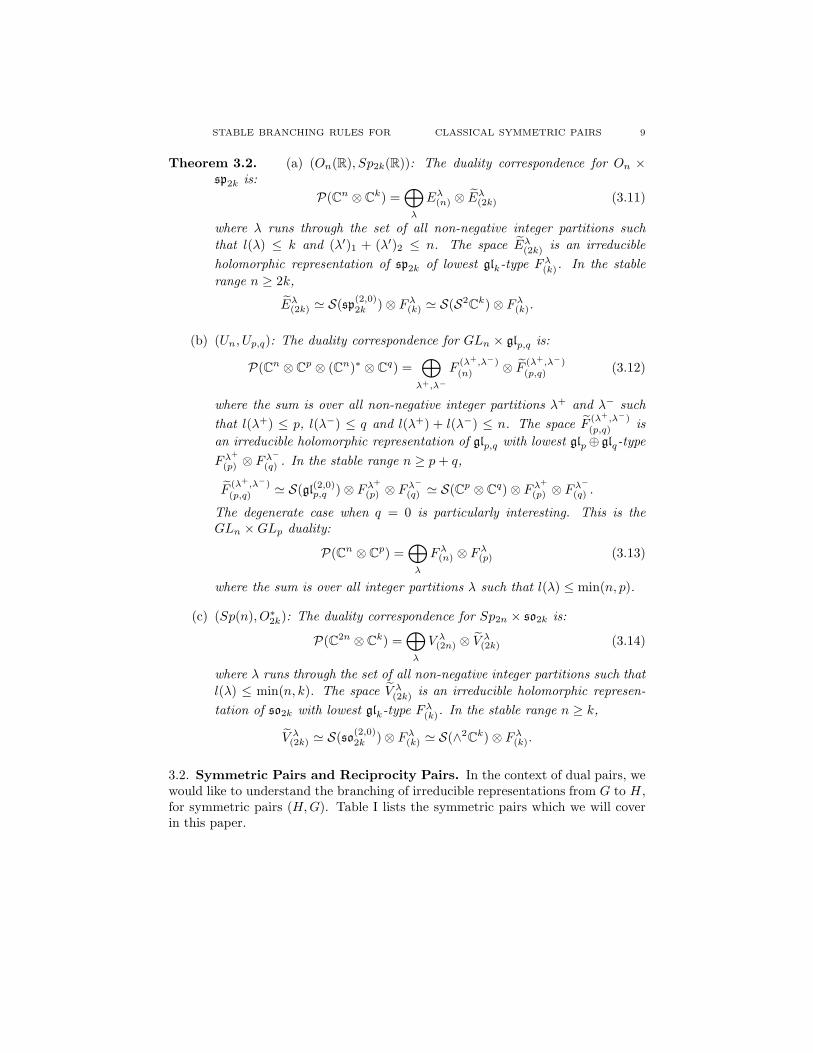
Theorem 3.2. (a) (On(R), Sp2k(R)): The duality correspondence for On ×sp2k is:
P(Cn ⊗ Ck) =
⊕
λ
Eλ(n) ⊗ Eλ(2k) (3.11)
where λ runs through the set of all non-negative integer partitions such
that l(λ) ≤ k and (λ′)1 + (λ′)2 ≤ n. The space Eλ(2k) is an irreducible
holomorphic representation of sp2k of lowest glk-type Fλ(k). In the stable
range n ≥ 2k,
Eλ(2k) ≃ S(sp(2,0)2k ) ⊗ Fλ(k) ≃ S(S2
Ck) ⊗ Fλ(k).
(b) (Un, Up,q): The duality correspondence for GLn × glp,q is:
P(Cn ⊗ Cp ⊗ (Cn)∗ ⊗ C
q) =⊕
λ+,λ−
F(λ+,λ−)(n) ⊗ F
(λ+,λ−)(p,q) (3.12)
where the sum is over all non-negative integer partitions λ+ and λ− such
that l(λ+) ≤ p, l(λ−) ≤ q and l(λ+) + l(λ−) ≤ n. The space F(λ+,λ−)(p,q) is
an irreducible holomorphic representation of glp,q with lowest glp⊕ glq-type
Fλ+
(p) ⊗ Fλ−
(q) . In the stable range n ≥ p+ q,
F(λ+,λ−)(p,q) ≃ S(gl(2,0)p,q ) ⊗ Fλ
+
(p) ⊗ Fλ−
(q) ≃ S(Cp ⊗ Cq) ⊗ Fλ
+
(p) ⊗ Fλ−
(q) .
The degenerate case when q = 0 is particularly interesting. This is theGLn ×GLp duality:
P(Cn ⊗ Cp) =
⊕
λ
Fλ(n) ⊗ Fλ(p) (3.13)
where the sum is over all integer partitions λ such that l(λ) ≤ min(n, p).
(c) (Sp(n), O∗2k): The duality correspondence for Sp2n × so2k is:
P(C2n ⊗ Ck) =
⊕
λ
V λ(2n) ⊗ V λ(2k) (3.14)
where λ runs through the set of all non-negative integer partitions such that
l(λ) ≤ min(n, k). The space V λ(2k) is an irreducible holomorphic represen-
tation of so2k with lowest glk-type Fλ(k). In the stable range n ≥ k,
V λ(2k) ≃ S(so(2,0)2k ) ⊗ Fλ(k) ≃ S(∧2
Ck) ⊗ Fλ(k).
3.2. Symmetric Pairs and Reciprocity Pairs. In the context of dual pairs, wewould like to understand the branching of irreducible representations from G to H ,for symmetric pairs (H,G). Table I lists the symmetric pairs which we will coverin this paper.
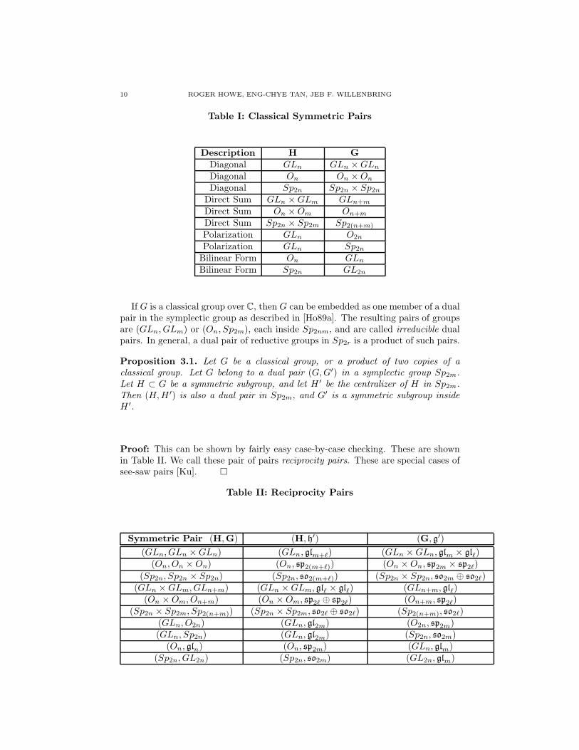
10 ROGER HOWE, ENG-CHYE TAN, JEB F. WILLENBRING
Table I: Classical Symmetric Pairs
Description H G
Diagonal GLn GLn ×GLnDiagonal On On ×OnDiagonal Sp2n Sp2n × Sp2n
Direct Sum GLn ×GLm GLn+m
Direct Sum On ×Om On+m
Direct Sum Sp2n × Sp2m Sp2(n+m)
Polarization GLn O2n
Polarization GLn Sp2n
Bilinear Form On GLnBilinear Form Sp2n GL2n
If G is a classical group over C, then G can be embedded as one member of a dualpair in the symplectic group as described in [Ho89a]. The resulting pairs of groupsare (GLn, GLm) or (On, Sp2m), each inside Sp2nm, and are called irreducible dualpairs. In general, a dual pair of reductive groups in Sp2r is a product of such pairs.
Proposition 3.1. Let G be a classical group, or a product of two copies of aclassical group. Let G belong to a dual pair (G,G′) in a symplectic group Sp2m.Let H ⊂ G be a symmetric subgroup, and let H ′ be the centralizer of H in Sp2m.Then (H,H ′) is also a dual pair in Sp2m, and G′ is a symmetric subgroup insideH ′.
Proof: This can be shown by fairly easy case-by-case checking. These are shownin Table II. We call these pair of pairs reciprocity pairs. These are special cases ofsee-saw pairs [Ku]. �
Table II: Reciprocity Pairs
Symmetric Pair (H,G) (H, h′) (G, g′)
(GLn, GLn ×GLn) (GLn, glm+ℓ) (GLn ×GLn, glm × glℓ)(On, On ×On) (On, sp2(m+ℓ)) (On ×On, sp2m × sp2ℓ)
(Sp2n, Sp2n × Sp2n) (Sp2n, so2(m+ℓ)) (Sp2n × Sp2n, so2m ⊕ so2ℓ)(GLn ×GLm, GLn+m) (GLn ×GLm, glℓ × glℓ) (GLn+m, glℓ)
(On ×Om, On+m) (On ×Om, sp2ℓ ⊕ sp2ℓ) (On+m, sp2ℓ)(Sp2n × Sp2m, Sp2(n+m)) (Sp2n × Sp2m, so2ℓ ⊕ so2ℓ) (Sp2(n+m), so2ℓ)
(GLn, O2n) (GLn, gl2m) (O2n, sp2m)(GLn, Sp2n) (GLn, gl2m) (Sp2n, so2m)
(On, gln) (On, sp2m) (GLn, glm)(Sp2n, GL2n) (Sp2n, so2m) (GL2n, glm)
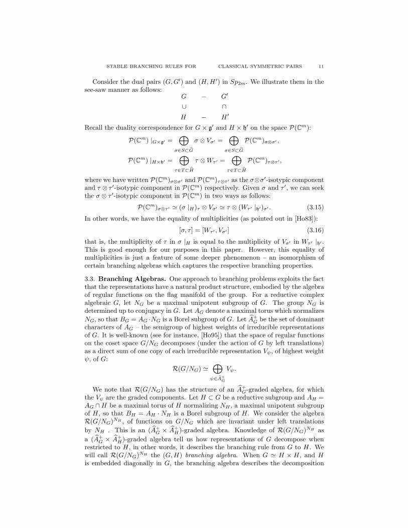
STABLE BRANCHING RULES FOR CLASSICAL SYMMETRIC PAIRS 11
Consider the dual pairs (G,G′) and (H,H ′) in Sp2m. We illustrate them in thesee-saw manner as follows:
G − G′
∪ ∩
H − H ′
Recall the duality correspondence for G× g′ and H × h′ on the space P(Cm):
P(Cm) |G×g′ =⊕
σ∈S⊂G
σ ⊗ Vσ′ =⊕
σ∈S⊂G
P(Cm)σ⊗σ′ ,
P(Cm) |H×h′ =⊕
τ∈T⊂H
τ ⊗Wτ ′ =⊕
τ∈T⊂H
P(Cm)τ⊗τ ′,
where we have written P(Cm)σ⊗σ′ and P(Cm)τ⊗τ ′ as the σ⊗σ′-isotypic componentand τ ⊗ τ ′-isotypic component in P(Cm) respectively. Given σ and τ ′, we can seekthe σ ⊗ τ ′-isotypic component in P(Cm) in two ways as follows:
P(Cm)σ⊗τ ′ ≃ (σ |H)τ ⊗ Vσ′ ≃ τ ⊗ (Wτ ′ |h′)σ′ . (3.15)
In other words, we have the equality of multiplicities (as pointed out in [Ho83]):
[σ, τ ] = [Wτ ′ , Vσ′ ] (3.16)
that is, the multiplicity of τ in σ |H is equal to the multiplicity of Vσ′ in Wτ ′ |h′ .This is good enough for our purposes in this paper. However, this equality ofmultiplicities is just a feature of some deeper phenomenon – an isomorphism ofcertain branching algebras which captures the respective branching properties.
3.3. Branching Algebras. One approach to branching problems exploits the factthat the representations have a natural product structure, embodied by the algebraof regular functions on the flag manifold of the group. For a reductive complexalgebraic G, let NG be a maximal unipotent subgroup of G. The group NG isdetermined up to conjugacy in G. Let AG denote a maximal torus which normalizes
NG, so that BG = AG ·NG is a Borel subgroup of G. Let A+G be the set of dominant
characters of AG – the semigroup of highest weights of irreducible representationsof G. It is well-known (see for instance, [Ho95]) that the space of regular functionson the coset space G/NG decomposes (under the action of G by left translations)as a direct sum of one copy of each irreducible representation Vψ, of highest weightψ, of G:
R(G/NG) ≃⊕
ψ∈A+
G
Vψ.
We note that R(G/NG) has the structure of an A+G-graded algebra, for which
the Vψ are the graded components. Let H ⊂ G be a reductive subgroup and AH =AG ∩H be a maximal torus of H normalizing NH , a maximal unipotent subgroupof H , so that BH = AH · NH is a Borel subgroup of H . We consider the algebraR(G/NG)NH , of functions on G/NG which are invariant under left translations
by NH . This is an (A+G × A+
H)-graded algebra. Knowledge of R(G/NG)NH as
a (A+G × A+
H)-graded algebra tell us how representations of G decompose whenrestricted to H , in other words, it describes the branching rule from G to H . Wewill call R(G/NG)NH the (G,H) branching algebra. When G ≃ H × H , and His embedded diagonally in G, the branching algebra describes the decomposition
12 ROGER HOWE, ENG-CHYE TAN, JEB F. WILLENBRING
of tensor products of representations of H , and we then call it the tensor productalgebra for H .
Let us explain briefly how branching algebras, dual pairs and reciprocity arerelated. For a reciprocity pair (G, g′), (H, h′), the duality correspondences aresubjugated to a correspondence in the space of harmonics H (see Theorem 3.1).Branching from holomorphic discrete series of h′ to g′ behaves very much like finite-dimensional representations in relation to their highest weights and is captured en-tirely by the branching from the lowest KH′ -type to KG′ . Although H is not analgebra, it can still be identified as a quotient algebra of P(Cm). With the G×KG′
as well as H × KH′ multiplicity-free decomposition of H, one allows HNH×NKG′
to be interpreted as a branching algebra from KH′ to KG′ as well as a branchingalgebra from G to H . This double interpretation solve two related branching prob-lems simultaneously. Classical invariant theory also provides a flexible approachwhich allows an inductive approach to the computation of branching algebras, andmakes evident natural connections between different branching algebras. We referto readers to [HTW] for more details.
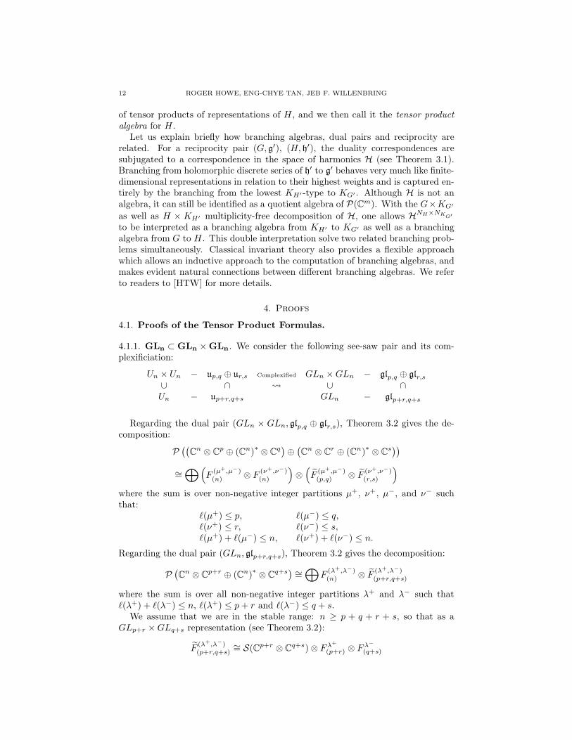
4. Proofs
4.1. Proofs of the Tensor Product Formulas.
4.1.1. GLn ⊂ GLn × GLn. We consider the following see-saw pair and its com-plexificiation:
Un × Un − up,q ⊕ ur,s Complexified GLn ×GLn − glp,q ⊕ glr,s∪ ∩ ∪ ∩Un − up+r,q+s GLn − glp+r,q+s
Regarding the dual pair (GLn × GLn, glp,q ⊕ glr,s), Theorem 3.2 gives the de-composition:
P((
Cn ⊗ C
p ⊕ (Cn)∗ ⊗ Cq)⊕(Cn ⊗ C
r ⊕ (Cn)∗ ⊗ Cs))
∼=⊕(
F(µ+,µ−)(n) ⊗ F
(ν+,ν−)(n)
)⊗(F
(µ+,µ−)(p,q) ⊗ F
(ν+,ν−)(r,s)
)
where the sum is over non-negative integer partitions µ+, ν+, µ−, and ν− suchthat:
ℓ(µ+) ≤ p, ℓ(µ−) ≤ q,ℓ(ν+) ≤ r, ℓ(ν−) ≤ s,ℓ(µ+) + ℓ(µ−) ≤ n, ℓ(ν+) + ℓ(ν−) ≤ n.
Regarding the dual pair (GLn, glp+r,q+s), Theorem 3.2 gives the decomposition:
P(Cn ⊗ C
p+r ⊕ (Cn)∗⊗ C
q+s)∼=⊕
F(λ+,λ−)(n) ⊗ F
(λ+,λ−)(p+r,q+s)
where the sum is over all non-negative integer partitions λ+ and λ− such thatℓ(λ+) + ℓ(λ−) ≤ n, ℓ(λ+) ≤ p+ r and ℓ(λ−) ≤ q + s.
We assume that we are in the stable range: n ≥ p + q + r + s, so that as aGLp+r ×GLq+s representation (see Theorem 3.2):
F(λ+,λ−)(p+r,q+s)
∼= S(Cp+r ⊗ Cq+s) ⊗ Fλ
+
(p+r) ⊗ Fλ−
(q+s)
STABLE BRANCHING RULES FOR CLASSICAL SYMMETRIC PAIRS 13
As a GLp ×GLq ×GLr ×GLs-representation, F(λ+,λ−)(p+r,q+s) is equivalent to:
S(Cp ⊗ Cq) ⊗ S(Cr ⊗ C
s) ⊗ S(Cp ⊗ Cs) ⊗ S(Cr ⊗ C
q) ⊗ Fλ+
(p+r) ⊗ Fλ−
(q+s)
Note that n ≥ p + q + r + s implies that n ≥ p + q and n ≥ r + s, so that (seeTheorem 3.2):
F(µ+,µ−)(p,q)
∼= S(Cp ⊗ Cq) ⊗ Fµ
+
(p) ⊗ Fµ−
(q)
and
F(ν+,ν−)(r,s)
∼= S(Cr ⊗ Cs) ⊗ F ν
+
(r) ⊗ F ν−
(s) .
Our see-saw pair implies (see (3.15)):[F
(µ+,µ−)(n) ⊗ F
(ν+,ν−)(n) , F
(λ+,λ−)(n)
]=[F
(λ+,λ−)(p+r,q+s), F
(µ+,µ−)(p,q) ⊗ F
(ν+,ν−)(r,s)
].
Using the fact that we are in the stable range:[F
(µ+,µ−)(n) ⊗ F
(ν+,ν−)(n) , F
(λ+,λ−)(n)
]
=[S(Cp ⊗ Cs) ⊗ S(Cr ⊗ Cq) ⊗ Fλ
+
(p+r) ⊗ Fλ−
(q+s), Fµ+
(p) ⊗ Fµ−
(q) ⊗ F ν+
(r) ⊗ F ν−
(s)
].
Next we will combine the standard decompositions:
Fλ+
(p+r)∼=⊕
cλ+
α1 α2Fα1
(p) ⊗ Fα2
(r)
Fλ−
(q+s)∼=⊕
cλ−
β1 β2F β1
(q) ⊗ F β2
(s)
with the multiplicity-free decompositions (see (3.12)):
S(Cp ⊗ Cs) ∼=
⊕F γ1(p) ⊗ F γ1(s)
S(Cr ⊗ Cq) ∼=
⊕F γ2(r) ⊗ F γ2(q).
This implies the result:[F
(µ+,µ−)(n) ⊗ F
(ν+,ν−)(n) , F
(λ+,λ−)(n)
]=∑
cλ+
α2 α1cµ
+
α1 γ1cν
−
γ1 β2cλ
−
β2 β1cµ
−
β1 γ2cν
+
γ2 α2.
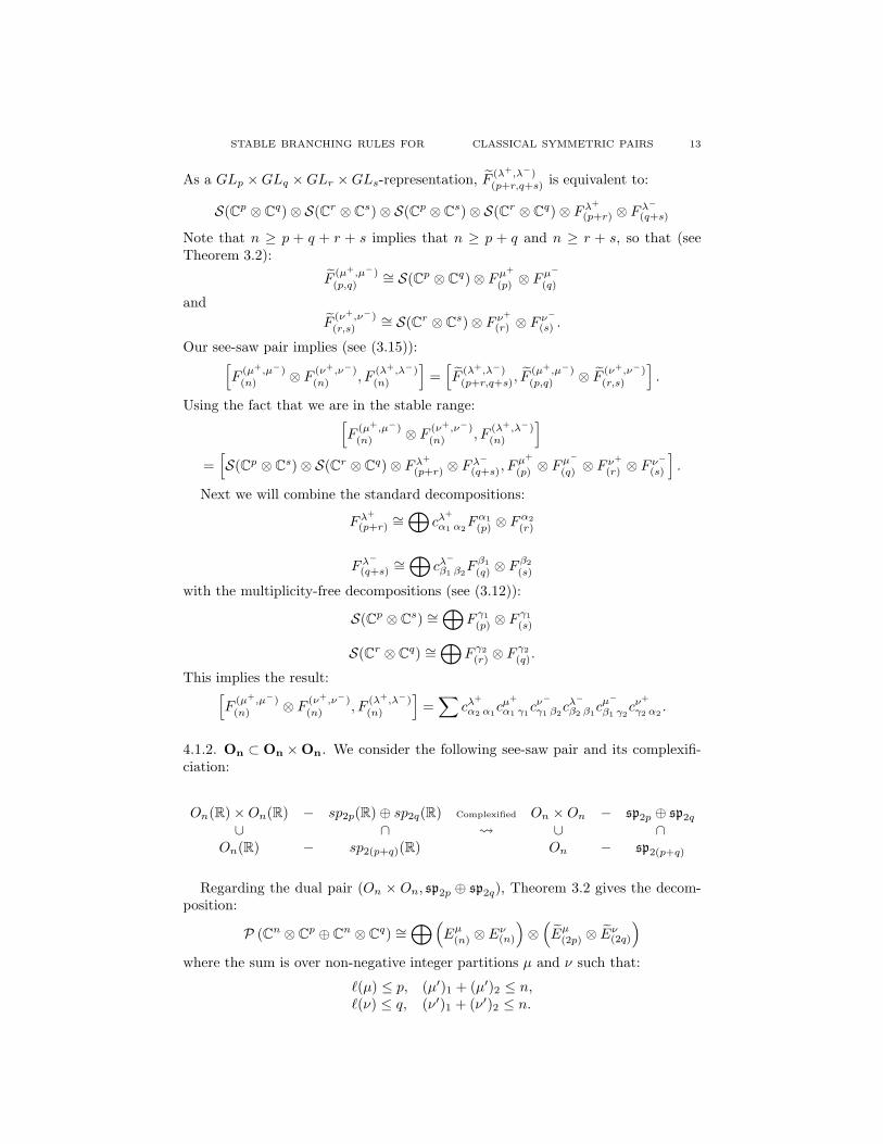
4.1.2. On ⊂ On × On. We consider the following see-saw pair and its complexifi-ciation:
On(R) ×On(R) − sp2p(R) ⊕ sp2q(R) Complexified On ×On − sp2p ⊕ sp2q
∪ ∩ ∪ ∩On(R) − sp2(p+q)(R) On − sp2(p+q)
Regarding the dual pair (On × On, sp2p ⊕ sp2q), Theorem 3.2 gives the decom-position:
P (Cn ⊗ Cp ⊕ C
n ⊗ Cq) ∼=
⊕(Eµ(n) ⊗ Eν(n)
)⊗(Eµ(2p) ⊗ Eν(2q)
)
where the sum is over non-negative integer partitions µ and ν such that:
ℓ(µ) ≤ p, (µ′)1 + (µ′)2 ≤ n,ℓ(ν) ≤ q, (ν′)1 + (ν′)2 ≤ n.
14 ROGER HOWE, ENG-CHYE TAN, JEB F. WILLENBRING
Regarding the dual pair (On, sp2(p+q)), Theorem 3.2 gives the decomposition:
P(Cn ⊗ C
p+q)∼=⊕
Eλ(n) ⊗ Eλ(2(p+q))
where the sum is over all non-negative integer partitions λ such that ℓ(λ) ≤ p+ q,and (λ′)1 + (λ′)2 ≤ n.
We assume that we are in the stable range: n ≥ 2(p + q), so that as a GLp+qrepresentation (see Theorem 3.2):
Eλ(2(p+q))∼= S(S2
Cp+q) ⊗ Fλ(p+q).
As a GLp ×GLq-representation, Eλ(2(p+q)) is equivalent to:
S(S2Cp) ⊗ S(S2
Cq) ⊗ S(Cp ⊗ C
q) ⊗ Fλ(p+q)
Note that n ≥ 2(p+ q) implies that n ≥ 2p and n ≥ 2q, so that (see Theorem 3.2):
Eµ(2p)∼= S(S2
Cp) ⊗ Fµ(p)
and
Eν(2q)∼= S(S2
Cq) ⊗ F ν(q).
Our see-saw pair implies (see (3.15)):[Eµ(n) ⊗ Eν(n), E
λ(n)] = [Eλ(2(p+q)), E
µ
(2p) ⊗ Eν(2q)
].
Using the fact that we are in the stable range:[Eλ(2(p+q)), E
µ
(2p) ⊗ Eν(2q)
]
=[S(S2
Cp) ⊗ S(S2
Cq) ⊗ S(Cp ⊗ C
q) ⊗ Fλ(p+q),S(S2Cp) ⊗ Fµ(p) ⊗ S(S2
Cq) ⊗ F ν(q)
]
=[S(Cp ⊗ C
q) ⊗ Fλ(p+q), Fµ
(p) ⊗ F ν(q)
].
Next we will combine the decomposition:
Fλ(p+q)∼=⊕
cλαβFα(p) ⊗ F β(q)
with the multiplicity-free decomposition (see (3.12)):
S(Cp ⊗ Cq) ∼=
⊕F γ(p) ⊗ F γ(q)
to obtain the result, but first note that in the above decompositions α, β, and γrange over all non-negative integer partitions such that ℓ(α) ≤ p, ℓ(β) ≤ q andℓ(γ) ≤ min(p, q). So we obtain:
[Eµ(n) ⊗ Eν(n), E
λ(n)
]=∑
α,β,γ
cλαβcµαγc
νβ γ
The above sum is over all non-negative integer partitions α, β, γ such that ℓ(α) ≤ p,ℓ(β) ≤ q and ℓ(γ) ≤ min(p, q), however, the support of the Littlewood-Richardsoncoefficients is contained inside the set of such (α, β, γ) when we choose p and q suchthat ℓ(λ) ≤ ⌊n/2⌋ := p+ q, with ℓ(µ) := p and ℓ(ν) := q.
STABLE BRANCHING RULES FOR CLASSICAL SYMMETRIC PAIRS 15
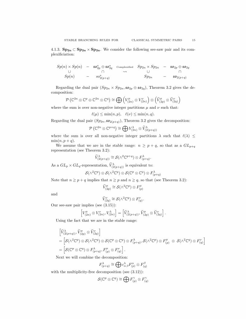
4.1.3. Sp2n ⊂ Sp2n × Sp2n. We consider the following see-saw pair and its com-plexificiation:
Sp(n) × Sp(n) − so∗2p ⊕ so∗2q Complexified Sp2n × Sp2n − so2p ⊕ so2q
∪ ∩ ∪ ∩Sp(n) − so∗2(p+q) Sp2n − so2(p+q)
Regarding the dual pair (Sp2n × Sp2n, so2p ⊕ so2q), Theorem 3.2 gives the de-composition:
P(C
2n ⊗ Cp ⊕ C
2n ⊗ Cq)∼=⊕(
V µ(2n) ⊗ V ν(2n)
)⊗(V µ(2p) ⊗ V ν(2q)
)
where the sum is over non-negative integer partitions µ and ν such that:
ℓ(µ) ≤ min(n, p), ℓ(ν) ≤ min(n, q).
Regarding the dual pair (Sp2n, so2(p+q)), Theorem 3.2 gives the decomposition:
P(C
2n ⊗ Cp+q)∼=⊕
V λ(2n) ⊗ V λ(2(p+q))
where the sum is over all non-negative integer partitions λ such that ℓ(λ) ≤min(n, p+ q).
We assume that we are in the stable range: n ≥ p + q, so that as a GLp+qrepresentation (see Theorem 3.2):
V λ(2(p+q))∼= S(∧2
Cp+q) ⊗ Fλ(p+q).
As a GLp ×GLq-representation, V λ(2(p+q)) is equivalent to:
S(∧2Cp) ⊗ S(∧2
Cq) ⊗ S(Cp ⊗ C
q) ⊗ Fλ(p+q)
Note that n ≥ p+ q implies that n ≥ p and n ≥ q, so that (see Theorem 3.2):
V µ(2p)∼= S(∧2
Cp) ⊗ Fµ(p)
andV ν(2q)
∼= S(∧2Cq) ⊗ F ν(q).
Our see-saw pair implies (see (3.15)):[V µ(2n) ⊗ V ν(2n), V
λ(2n)
]=[V λ(2(p+q)), V
µ
(2p) ⊗ V ν(2q)
].
Using the fact that we are in the stable range:
[V λ(2(p+q)), V
µ
(2p) ⊗ V ν(2q)
]
=[S(∧2
Cp) ⊗ S(∧2
Cq) ⊗ S(Cp ⊗ C
q) ⊗ Fλ(p+q),S(∧2Cp) ⊗ Fµ(p) ⊗ S(∧2
Cq) ⊗ F ν(q)
]
=[S(Cp ⊗ C
q) ⊗ Fλ(p+q), Fµ
(p) ⊗ F ν(q)
].
Next we will combine the decomposition:
Fλ(p+q)∼=⊕
cλαβFα(p) ⊗ F β(q)
with the multiplicity-free decomposition (see (3.12)):
S(Cp ⊗ Cq) ∼=
⊕F γ(p) ⊗ F γ(q)
16 ROGER HOWE, ENG-CHYE TAN, JEB F. WILLENBRING
to obtain the result, but first note that in the above decompositions α, β, and γrange over all non-negative integer partitions such that ℓ(α) ≤ p, ℓ(β) ≤ q andℓ(γ) ≤ min(p, q). So we obtain:
[V µ(2n) ⊗ V ν(2n), V
λ(2n)
]=∑
α,β,γ
cλαβcµα γc
νβ γ
The above sum is over all non-negative integer partitions α, β, γ such that ℓ(α) ≤ p,ℓ(β) ≤ q and ℓ(γ) ≤ min(p, q), however, the support of the Littlewood-Richardsoncoefficients is contained inside the set of such (α, β, γ) when we choose p and q suchthat ℓ(λ) ≤ ⌊n/2⌋ := p+ q, with ℓ(µ) := p and ℓ(ν) := q.
4.2. Proofs of the Direct Sum Branching Rules.
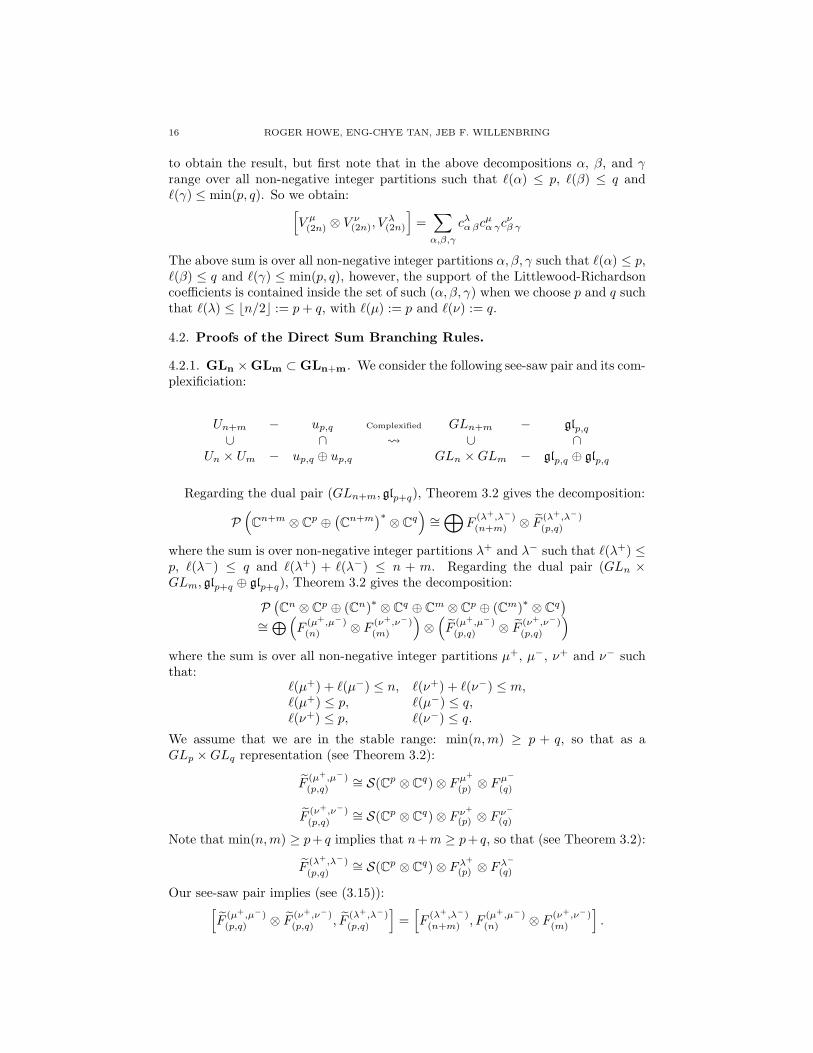
4.2.1. GLn × GLm ⊂ GLn+m. We consider the following see-saw pair and its com-plexificiation:
Un+m − up,q Complexified GLn+m − glp,q∪ ∩ ∪ ∩
Un × Um − up,q ⊕ up,q GLn ×GLm − glp,q ⊕ glp,q
Regarding the dual pair (GLn+m, glp+q), Theorem 3.2 gives the decomposition:
P(Cn+m ⊗ C
p ⊕(Cn+m
)∗⊗ C
q)∼=⊕
F(λ+,λ−)(n+m) ⊗ F
(λ+,λ−)(p,q)
where the sum is over non-negative integer partitions λ+ and λ− such that ℓ(λ+) ≤p, ℓ(λ−) ≤ q and ℓ(λ+) + ℓ(λ−) ≤ n + m. Regarding the dual pair (GLn ×GLm, glp+q ⊕ glp+q), Theorem 3.2 gives the decomposition:
P(Cn ⊗ Cp ⊕ (Cn)∗ ⊗ Cq ⊕ Cm ⊗ Cp ⊕ (Cm)∗ ⊗ Cq
)
∼=⊕(
F(µ+,µ−)(n) ⊗ F
(ν+,ν−)(m)
)⊗(F
(µ+,µ−)(p,q) ⊗ F
(ν+,ν−)(p,q)
)
where the sum is over all non-negative integer partitions µ+, µ−, ν+ and ν− suchthat:
ℓ(µ+) + ℓ(µ−) ≤ n, ℓ(ν+) + ℓ(ν−) ≤ m,ℓ(µ+) ≤ p, ℓ(µ−) ≤ q,ℓ(ν+) ≤ p, ℓ(ν−) ≤ q.
We assume that we are in the stable range: min(n,m) ≥ p + q, so that as aGLp ×GLq representation (see Theorem 3.2):
F(µ+,µ−)(p,q)
∼= S(Cp ⊗ Cq) ⊗ Fµ
+
(p) ⊗ Fµ−
(q)
F(ν+,ν−)(p,q)
∼= S(Cp ⊗ Cq) ⊗ F ν
+
(p) ⊗ F ν−
(q)
Note that min(n,m) ≥ p+ q implies that n+m ≥ p+ q, so that (see Theorem 3.2):
F(λ+,λ−)(p,q)
∼= S(Cp ⊗ Cq) ⊗ Fλ
+
(p) ⊗ Fλ−
(q)
Our see-saw pair implies (see (3.15)):[F
(µ+,µ−)(p,q) ⊗ F
(ν+,ν−)(p,q) , F
(λ+,λ−)(p,q)
]=[F
(λ+,λ−)(n+m) , F
(µ+,µ−)(n) ⊗ F
(ν+,ν−)(m)
].
STABLE BRANCHING RULES FOR CLASSICAL SYMMETRIC PAIRS 17
Using the fact that we are in the stable range:[F
(µ+,µ−)(p,q) ⊗ F
(ν+,ν−)(p,q) , F
(λ+,λ−)(p,q)
]
=[(
S(Cp ⊗ Cq) ⊗ Fµ
+
(p) ⊗ Fµ−
(q)
)⊗(S(Cp ⊗ C
q) ⊗ F ν+
(p) ⊗ F ν−
(q)
),S(Cp ⊗ C
q) ⊗ Fλ+
(p) ⊗ Fλ−
(q)
]
=[S(Cp ⊗ C
q) ⊗ Fµ+
(p) ⊗ Fµ−
(q) ⊗ F ν+
(p) ⊗ F ν−
(q) , Fλ+
(p) ⊗ Fλ−
(q)
].
Next combine the above decomposition with (see (3.12)):
S(Cp ⊗ Cq) ∼=
⊕F δ(p) ⊗ F δ(q)
where the sum is over all non-negative integer partitions δ with at most min(p, q)parts. We then obtain:
[F
(λ+,λ−)(n+m) , F
(µ+,µ−)(n) ⊗ F
(ν+,ν−)(m)
]
=[(⊕
δ Fδ(p) ⊗ F δ(q)
)⊗(Fµ
+
(p) ⊗ Fµ−
(q)
)⊗(F ν
+
(p) ⊗ F ν−
(q)
), Fλ
+
(p) ⊗ Fλ−
(q)
].
We combine this fact with the following two tensor product decompostions:
Fµ+
(p) ⊗ F ν+
(p)∼=
⊕cγ
+
µ+ ν+Fγ+
(p) and Fµ−
(q) ⊗ F ν−
(q)∼=
⊕cγ
−
µ− ν−F γ
−
(q)
(where γ+ and γ− have at most p and q parts respectively) and then tensor theconstituents with F δ(p) ⊗ F δ(q),
F γ+
(p) ⊗ F δ(p)∼=
⊕cλ
+
γ+ δFλ
+
(p) and F γ−
(q) ⊗ F δ(q)∼=
⊕cλ
−
γ− δFλ
−
(q)
to obtain the result.
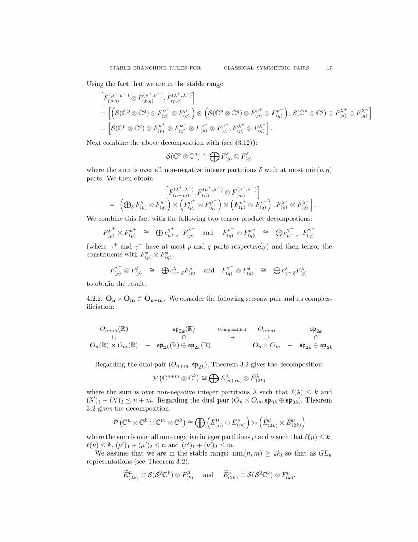
4.2.2. On × Om ⊂ On+m. We consider the following see-saw pair and its complex-ificiation:
On+m(R) − sp2k(R) Complexified On+m − sp2k
∪ ∩ ∪ ∩On(R) ×Om(R) − sp2k(R) ⊕ sp2k(R) On ×Om − sp2k ⊕ sp2k
Regarding the dual pair (On+m, sp2k), Theorem 3.2 gives the decomposition:
P(Cn+m ⊗ C
k)∼=⊕
Eλ(n+m) ⊗ Eλ(2k)
where the sum is over non-negative integer partitions λ such that ℓ(λ) ≤ k and(λ′)1 + (λ′)2 ≤ n +m. Regarding the dual pair (On × Om, sp2k ⊕ sp2k), Theorem3.2 gives the decomposition:
P(Cn ⊗ C
k ⊕ Cm ⊗ C
k)∼=⊕(
Eµ(n) ⊗ Eν(m)
)⊗(Eµ(2k) ⊗ Eν(2k)
)
where the sum is over all non-negative integer partitions µ and ν such that ℓ(µ) ≤ k,ℓ(ν) ≤ k, (µ′)1 + (µ′)2 ≤ n and (ν′)1 + (ν′)2 ≤ m.
We assume that we are in the stable range: min(n,m) ≥ 2k, so that as GLkrepresentations (see Theorem 3.2):
Eµ(2k)∼= S(S2Ck) ⊗ Fµ(k) and Eν(2k)
∼= S(S2Ck) ⊗ F ν(k).

18 ROGER HOWE, ENG-CHYE TAN, JEB F. WILLENBRING
Note that min(n,m) ≥ 2k implies that n+m ≥ 2k, so that (see Theorem 3.2):
Eλ(2k)∼= S(S2
Ck) ⊗ Fλ(k)
Our see-saw pair implies (see (3.15)):[Eµ(2k) ⊗ Eν(2k), E
λ(2k)
]=[Eλ(n+m), E
µ
(n) ⊗ F ν(m)
].
Using the fact that we are in the stable range:[Eµ(2k) ⊗ Eν(2k), E
λ(2k)
]=[(
S(S2Ck) ⊗ Fµ(k)
)⊗(S(S2
Ck) ⊗ F ν(k)
),S(S2
Ck) ⊗ Fλ(k)
]
=[S(S2
Ck) ⊗ Fµ(k) ⊗ F ν(k), F
λ(k)
].
Next combine with the well-known multiplicity-free decomposition (see for instance,Theorem 3.1 of [Ho95] on page 32):
S(S2Ck) ∼=
⊕F 2δ
(k)
where the sum is over all non-negative integer partitions δ with at most k parts.We then obtain:
[Eλ(n+m), E
µ
(n) ⊗ Eν(m)
]=
[(⊕
δ
F 2δ(k)
)⊗ Fµ(k) ⊗ F ν(k), F
λ(k)
].
Combine this fact with the following two tensor product decompositions:
Fµ(k) ⊗ F ν(k)∼=
⊕cγµ νF
γ
(k) and F γ(k) ⊗ F 2δ(k)
∼=⊕cλγ 2δF
λ(k)
(where γ is a non-negative integer partition with at most k parts) and the resultfollows.
4.2.3. Sp2n × Sp2m ⊂ Sp2(n+m). We consider the following see-saw pair and itscomplexificiation:
Sp(n+m) − so∗2k Complexified Sp2(n+m) − so2k
∪ ∩ ∪ ∩Sp(n) × Sp(m) − so∗2k ⊕ so∗2k Sp2n × Sp2m − so2k ⊕ so2k
Regarding the dual pair (Sp2(n+m), so2k), Theorem 3.2 gives the decomposition:
P(
C2(n+m) ⊗ C
k)∼=⊕
V λ(2(n+m)) ⊗ V λ(2k)
where the sum is over non-negative integer partitions λ such thatℓ(λ) ≤ min(n+m, k). Regarding the dual pair (Sp2n×Sp2m, so2k⊕so2k), Theorem3.2 gives the decomposition:
P(C
2n ⊗ Ck ⊕ C
2m ⊗ Ck)∼=⊕(
V µ(2n) ⊗ V ν(2m)
)⊗(V µ(2k) ⊗ V ν(2k)
)
where the sum is over all non-negative integer partitions µ and ν such that ℓ(µ) ≤min(n, k), ℓ(ν) ≤ min(n, k).
We assume that we are in the stable range: min(n,m) ≥ k, so that as GLkrepresentations (see Theorem 3.2):
V µ(2k)∼= S(∧2Ck) ⊗ Fµ(k) and V ν(2k)
∼= S(∧2Ck) ⊗ F ν(k).
STABLE BRANCHING RULES FOR CLASSICAL SYMMETRIC PAIRS 19
Note that min(n,m) ≥ k implies that n+m ≥ k, so that (see Theorem 3.2):
V λ(2k)∼= S(∧2
Ck) ⊗ Fλ(k)
Our see-saw pair implies (see (3.15)):[V µ(2k) ⊗ V ν(2k), V
λ(2k)
]=[V λ(n+m), V
µ
(n) ⊗ V ν(m)
].
Using the fact that we are in the stable range:[V µ(2k) ⊗ V ν(2k), V
λ(2k)
]=
[(S(∧2
Ck) ⊗ Fµ(k)
)⊗(S(∧2
Ck) ⊗ F ν(k)
),S(∧2
Ck) ⊗ Fλ(k)
]
=[S(∧2
Ck) ⊗ Fµ(k) ⊗ F ν(k), F
λ(k)
].
Next combine with the well-known multiplicity-free decomposition (see for instance,Theorem 3.8.1 of [Ho95] on page 44):
S(∧2Ck) ∼=
⊕F
(2δ)′
(k)
where the sum is over all non-negative integer partitions δ such that (2δ)′ has atmost k parts. We then obtain:
[V λ(2(n+m)), V
µ
(2n) ⊗ V ν(2m)
]=
[(⊕
δ
F(2δ)′
(k)
)⊗ Fµ(k) ⊗ F ν(k), F
λ(k)
].
Combine this fact with the following two tensor product decompositions:
Fµ(k) ⊗ F ν(k)∼=
⊕cγµνF
γ
(k) and F γ(k) ⊗ F(2δ)′
(k)∼=
⊕cλγ (2δ)′F
λ(k)
(where γ is a non-negative integer partition with at most k parts) and the resultfollows.
4.3. Proofs of the Polarization Branching Rules.
4.3.1. GLn ⊂ O2n. We consider the following see-saw pair and its complexificia-tion:
O2n(R) − sp2k(R) Complexified O2n − sp2k
∪ ∩ ∪ ∩U(n) − uk,k GLn − glk,k
Regarding the dual pair (O2n, sp2k), Theorem 3.2 gives the decomposition:
P(C
2n ⊗ Ck)∼=⊕
Eλ(2n) ⊗ Eλ(2k)
where the sum is over all non-negative integer partitions λ such that ℓ(λ) ≤ k and(λ′)1 + (λ′)2 ≤ 2n. Since the standard O2n representation C2n ≃ Cn ⊕ (Cn)∗ asa GLn representation, regarding the dual pair (GLn, glk,k), Theorem 3.2 gives thedecomposition:
P(Cn ⊗ C
k ⊗ (Cn)∗⊗ C
k)∼=⊕
F(µ+,µ−)(n) ⊗ F
(µ+,µ−)(k,k)
where the sum is over non-negative integer partitions µ+ and µ− with at most kparts such that ℓ(µ+) + ℓ(µ−) ≤ n.
20 ROGER HOWE, ENG-CHYE TAN, JEB F. WILLENBRING
We assume that we are in the stable range: n ≥ 2k, so that as a GLk × GLkrepresentation (see Theorem 3.2):
F(µ+,µ−)(k,k)
∼= S(Ck ⊗ Ck) ⊗ Fµ
+
(k) ⊗ Fµ−
(k) .
Note that n ≥ 2k implies that n ≥ k, so that as GLk representations (see Theorem3.2):
Eλ(2k)∼= S(S2
Ck) ⊗ Fλ(k)
Our see-saw pair implies (see (3.15)):[F
(µ+,µ−)(k,k) , Eλ(2k)
]=[Eλ(2n), F
(µ+,µ−)(n)
].
Using the fact that we are in the stable range:[F
(µ+,µ−)(k,k) , Eλ(2k)
]=
[S(Ck ⊗ C
k) ⊗ Fµ+
(k) ⊗ Fµ−
(k) ,S(S2Ck) ⊗ Fλ(k)
]
=[S(∧2
Ck) ⊗ Fµ
+
(k) ⊗ Fµ−
(k) , Fλ(k)
].
Note that in the above we used the fact that as a GLk-representation,⊗2Ck ∼= S2Ck ⊕ ∧2Ck.
Next combine with the well-known multiplicity-free decomposition:
S(∧2Ck) ∼=
⊕F
(2δ)′
(k)
where the sum is over all non-negative integer partitions δ such that (2δ)′ has atmost k parts. We then obtain:
[Eλ(2n), F
(µ+,µ−)(n)
]=
[(⊕
δ
F(2δ)′
(k)
)⊗ Fµ
+
(k) ⊗ Fµ−
(k) , Fλ(k)
].
Combine this fact with the following two tensor product decompositions:
Fµ+
(k) ⊗ Fµ−
(k)∼=
⊕cγµ+ µ−
F γ(k) and F γ(k) ⊗ F(2δ)′
(k)∼=
⊕cλγ (2δ)′F
λ(k)
(where γ is a non-negative integer partition with at most k parts) and the resultfollows.
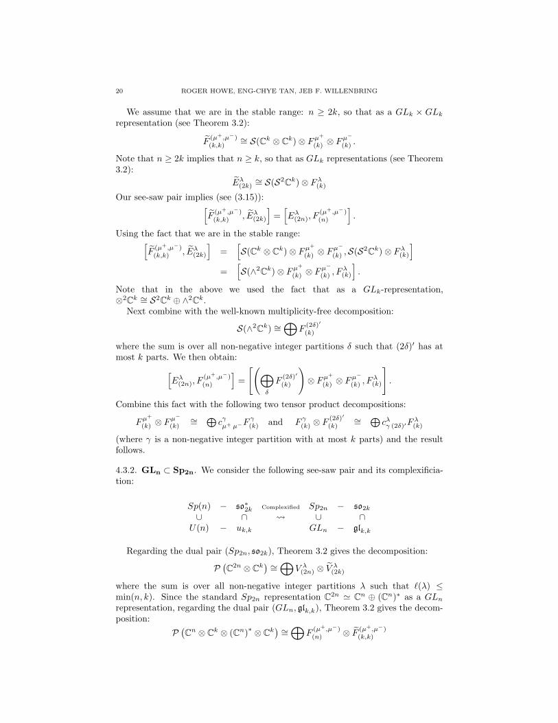
4.3.2. GLn ⊂ Sp2n. We consider the following see-saw pair and its complexificia-tion:
Sp(n) − so∗2k Complexified Sp2n − so2k
∪ ∩ ∪ ∩U(n) − uk,k GLn − glk,k
Regarding the dual pair (Sp2n, so2k), Theorem 3.2 gives the decomposition:
P(C
2n ⊗ Ck)∼=⊕
V λ(2n) ⊗ V λ(2k)
where the sum is over all non-negative integer partitions λ such that ℓ(λ) ≤min(n, k). Since the standard Sp2n representation C2n ≃ Cn ⊕ (Cn)∗ as a GLnrepresentation, regarding the dual pair (GLn, glk,k), Theorem 3.2 gives the decom-position:
P(Cn ⊗ C
k ⊗ (Cn)∗⊗ C
k)∼=⊕
F(µ+,µ−)(n) ⊗ F
(µ+,µ−)(k,k)
STABLE BRANCHING RULES FOR CLASSICAL SYMMETRIC PAIRS 21
where the sum is over non-negative integer partitions µ+ and µ− with at most kparts such that ℓ(µ+) + ℓ(µ−) ≤ n.
We assume that we are in the stable range: n ≥ 2k, so that as GLk × GLkrepresentations (see Theorem 3.2):
F(µ+,µ−)(k,k)
∼= S(Ck ⊗ Ck) ⊗ Fµ
+
(k) ⊗ Fµ−
(k) .
Note that n ≥ 2k implies that n ≥ k, so that as a GLk representation (see Theorem3.2):
V λ(2k)∼= S(∧2
Ck) ⊗ Fλ(k)
Our see-saw pair implies (see (3.15)):[F
(µ+,µ−)(k,k) , V λ(2k)
]=[V λ(2n), F
(µ+,µ−)(n)
].
Using the fact that we are in the stable range:[F
(µ+,µ−)(k,k) , Eλ(2k)
]=
[S(Ck ⊗ C
k) ⊗ Fµ+
(k) ⊗ Fµ−
(k) ,S(∧2Ck) ⊗ Fλ(k)
]
=[S(S2
Ck) ⊗ Fµ
+
(k) ⊗ Fµ−
(k) , Fλ(k)
].
Note that in the above we used the fact that as a GLk-representation,⊗2Ck ∼= S2Ck ⊕ ∧2Ck.
Next combine with the well-known multiplicity-free decomposition:
S(S2Ck) ∼=
⊕F 2δ
(k)
where the sum is over all non-negative integer partitions δ with at most k parts.We then obtain:
[V λ(2n), F
(µ+,µ−)(n)
]=
[(⊕
δ
F 2δ(k)
)⊗ Fµ
+
(k) ⊗ Fµ−
(k) , Fλ(k)
].
Combine this fact with the following two tensor product decompositions:
Fµ+
(k) ⊗ Fµ−
(k)∼=
⊕cγµ+ µ−
F γ(k) and F γ(k) ⊗ F 2δ(k)
∼=⊕cλγ 2δF
λ(k)
(where γ is a non-negative integer partition with at most k parts) and the resultfollows.
4.4. Proofs of the Bilinear Form Branching Rules.
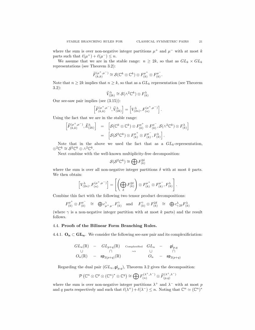
4.4.1. On ⊂ GLn. We consider the following see-saw pair and its complexificiation:
GLn(R) − GLp+q(R) Complexified GLn − glp,q∪ ∩ ∪ ∩
On(R) − sp2(p+q)(R) On − sp2(p+q)
Regarding the dual pair (GLn, glp,q), Theorem 3.2 gives the decomposition:
P(Cn ⊗ C
p ⊗ (Cn)∗ ⊗ Cq)∼=⊕
F(λ+,λ−)(n) ⊗ F
(λ+,λ−)(p,q)
where the sum is over non-negative integer partitions λ+ and λ− with at most pand q parts respectively and such that ℓ(λ+)+ ℓ(λ−) ≤ n. Noting that C
n ≃ (Cn)∗

22 ROGER HOWE, ENG-CHYE TAN, JEB F. WILLENBRING
as an On representation, regarding the dual pair (On, sp2(p+q)), Theorem 3.2 givesthe decomposition:
P(Cn ⊗ C
p+q)∼=⊕
Eλ(n) ⊗ Eλ(2(p+q))
where the sum is over all non-negative integer partitions λ such that ℓ(λ) ≤ p+ qand (λ′)1 + (λ′)2 ≤ n.
We assume that we are in the stable range: n ≥ 2(p + q), so that as GLp+qrepresentations (see Theorem 3.2):
Eµ(2(p+q))∼= S(S2
Cp+q) ⊗ Fµ(p+q).
Note that n ≥ 2(p+q) implies that n ≥ p+q, so that as GLp×GLq representations(see Theorem 3.2):
F(λ+,λ−)(p,q)
∼= S(Cp ⊗ Cq) ⊗ Fλ
+
(p) ⊗ Fλ−
(q) .
Our see-saw pair implies (see (3.15):[Eµ(2(p+q)), F
(λ+,λ−)(p,q)
]=[F
(λ+,λ−)(n) , Eµ(n)
].
Using the fact that we are in the stable range:[Eµ(2(p+q)), F
(λ+,λ−)(p,q)
]
=[S(S2
Cp+q) ⊗ Fµ(p+q),S(Cp ⊗ C
q) ⊗ Fλ+
(p) ⊗ Fλ−
(q)
]
=[S(S2
Cp ⊕ S2
Cq ⊕ C
p ⊗ Cq) ⊗ Fµ(p+q),S(Cp ⊗ C
q) ⊗ Fλ+
(p) ⊗ Fλ−
(q)
]
=[S(S2
Cp) ⊗ S(S2
Cq) ⊗ Fµ(p+q), F
λ+
(p) ⊗ Fλ−
(q)
]
Next we combine the decompositions:
Fµ(p+q)∼=⊕
cµαβFα(p) ⊗ F β(q),
with the multiplicity-free decompositions:
S(S2Cp) ∼=
⊕F 2γ
(p) and S(S2Cq) ∼=
⊕F 2δ
(q)
where the sums are over all non-negative integer partitions γ and δ with at most pand q parts respectively. We then obtain:[F
(λ+,λ−)(n) , Eµ(n)
]=[(⊕
F 2γ(p)
)⊗(⊕
F 2δ(q)
)⊗(⊕
cµαβFα(p) ⊗ F β(q)
), Fλ
+
(p) ⊗ Fλ−
(q)
].
Combine this fact with the following two tensor product decompositions:
Fα(p) ⊗ F 2γ(p)
∼=⊕cλ
+
α 2γFλ+
(p) and F β(q) ⊗ F 2δ(q)
∼=⊕cλ
−
β 2δFλ−
(q)
and the result follows.
4.4.2. Sp2n ⊂ GL2n. We consider the following see-saw pair and its complexifici-ation:
U2n − up,q Complexified GL2n − glp,q∪ ∩ ∪ ∩
Sp(n) − so∗2(p+q) Sp2n − so2(p+q)
STABLE BRANCHING RULES FOR CLASSICAL SYMMETRIC PAIRS 23
Regarding the dual pair (GL2n, glp,q), Theorem 3.2 gives the decomposition:
P(
C2n ⊗ C
p ⊗(C
2n)∗
⊗ Cq)∼=⊕
F(λ+,λ−)(2n) ⊗ F
(λ+,λ−)(p,q)
where the sum is over non-negative integer partitions λ+ and λ− with at most p andq parts respectively and such that ℓ(λ+) + ℓ(λ−) ≤ 2n. Noting that (C2n)∗ ≃ C2n
as Sp2n modules, regarding the dual pair (Sp2n, so2(p+q)), Theorem 3.2 gives thedecomposition:
P(C
2n ⊗ Cp+q)∼=⊕
V λ(2n) ⊗ V λ(2(p+q))
where the sum is over all non-negative integer partitions λ such that ℓ(λ) ≤min(2n, p+ q).
We assume that we are in the stable range: n ≥ p + q, so that as GLp+qrepresentations (see Theorem 3.2):
V µ(2(p+q))∼= S(∧2
Cp+q) ⊗ Fµ(p+q)
Note that n ≥ p+ q implies that 2n ≥ p+ q, so that as GLp×GLq representations(see Theorem 3.2):
F(λ+,λ−)(p,q)
∼= S(Cp ⊗ Cq) ⊗ Fλ
+
(p) ⊗ Fλ−
(q)
Our see-saw pair implies (see (3.15)):[V µ(2(p+q)), F
(λ+,λ−)(p,q)
]=[F
(λ+,λ−)(2n) , V µ(2n)
].
Using the fact that we are in the stable range:[V µ(2(p+q)), F
(λ+,λ−)(p,q)
]
=[S(∧2
Cp+q) ⊗ Fµ(p+q),S(Cp ⊗ C
q) ⊗ Fλ+
(p) ⊗ Fλ−
(q)
]
=[S(∧2
Cp ⊕ ∧2
Cq ⊕ C
p ⊗ Cq) ⊗ Fµ(p+q),S(Cp ⊗ C
q) ⊗ Fλ+
(p) ⊗ Fλ−
(q)
]
=[S(∧2
Cp) ⊗ S(∧2
Cq) ⊗ Fµ(p+q), F
λ+
(p) ⊗ Fλ−
(q)
]
Next we combine the decompositions:
Fµ(p+q)∼=⊕
cµαβFα(p) ⊗ F β(q),
with the multiplicity-free decompositions:
S(∧2Cp) ∼=
⊕F
(2γ)′
(p) and S(∧2Cq) ∼=
⊕F
(2δ)′
(q) ,
where the sums are over all non-negative integer partitions γ and δ such that (2γ)′
and (2δ)′ have at most p and q parts respectively. We then obtain:[F
(λ+,λ−)(2n) , V µ(2n)
]=[(⊕
F(2γ)′
(p)
)⊗(⊕
F(2δ)′
(q)
)⊗(⊕
cµαβFα(p) ⊗ F β(q)
), Fλ
+
(p) ⊗ Fλ−
(q)
].
Combine with the following two tensor product decompositions:
Fα(p) ⊗ F(2γ)′
(p)∼=
⊕cλ
+
α (2γ)′Fλ+
(p) and F β(q) ⊗ F(2δ)′
(q)∼=
⊕cλ
−
β (2δ)′Fλ−
(q)
and the result follows.
24 ROGER HOWE, ENG-CHYE TAN, JEB F. WILLENBRING
References
[BKW] G. R. E. Black, R. C. King, B.G. Wybourne Kronecker products for compact semisimpleLie groups, J. Phys. A 16 (1983), no. 8, 1555–1589.
[CGR] Y. Chen, A. Garsia and J. Remmel, Algorithms for plethysm in combinatorics and alge-bra, Contemp. Math. 24, AMS, Providence, R.I. (1984), 109 – 153.
[EHW] T. Enright, R. Howe, and N. Wallach, Classification of unitary highest weight modules, inRepresentation Theory of Reductive Groups (P.C. Trombi, Ed.), pp. 97 – 144, Birkhauser,Boston, 1983.
[EW1] T. Enright and J. Willenbring, Hilbert series, Howe duality, and branching rules forclassical groups. To appear in the Annals of Mathematics.
[EW2] T. Enright and J. Willenbring, Hilbert series, Howe duality, and branching rules. WithThomas J. Enright, Proceedings of the National Academy of Sciences. 100 (2003), no.2,434–437.
[Fu] W. Fulton, Young Tableaux, Cambridge University Press, Cambridge, UK, 1997.[GW] R. Goodman and N. R. Wallach, Representations and Invariants of the Classical Groups,
Cambridge U. Press, 1998.[HC] Harish-Chandra, Representations of semisimple Lie groups IV/V/VI, Amer J. Math. 77
(1955), 743 – 777; Trans. Amer. Math. Soc. 78 (1956), 1 – 41; Amer J. Math. 78 (1956),564 – 628.
[Ho83] R. Howe, Reciprocity laws in the theory of dual pairs, in Representation Theory of Re-ductive Groups, Prog. in Math. 40, P. Trombi, ed., Birkhauser, Boston (1983), 159 –175.
[Ho89a] R. Howe, Remarks on classical invariant theory, Trans. Amer. Math. Soc. 313 (1989),539 – 570.
[Ho89b] R. Howe, Transcending classical invariant theory, J. Amer. Math. Soc. 2 (1989), 535 –552.
[Ho95] R. Howe, Perspectives on Invariant Theory, The Schur Lectures, I. Piatetski-Shapiro and
S. Gelbart (eds.), Israel Mathematical Conference Proceedings, 1995, 1 – 182.[HTW] R. Howe, E-C. Tan and J Willenbring, Reciprocity algebras and branching for classical
symmetric pairs, in preparation.[JK] G. James and A. Kerber, The Representation Theory of the Symmetric Group, Enc. of
Math. and App. 16, Addison-Wesley, Reading, MA., 1981.[KV] M. Kashiwara and M. Vergne, On the Segal-Shale-Weil representations and harmonic
polynomials, Invent. Math. 44 (1978), 1 – 47.[Ki1] R. C. King, Modification rules and products of irreducible representations for the unitary,
orthogonal, and symplectic groups, J. Math. Phys. 12 (1971), 1588-1598.[Ki2] R. C. King, Branching rules for classical Lie gorups using tensor and spinor methods,
J. Phys. A 8 (1975), 429-449.[Kn86] A. W. Knapp, Representation Theory of Semisimple Groups: An Overview Based on
Examples, Princeton University Press, Princeton, NJ, 1986.[Kn01] A. W. Knapp, Branching theorems for compact symmetric spaces, Represent. Theory 5
(2001), 404 – 436.[Kn02] A. W. Knapp, Lie Groups Beyond An Introduction, Second edition, Progress in Mathe-
matics 140, Birkhuser Boston, Inc., Boston, MA, 2002.[KT] K. Koike and I. Terada, Young diagrammatic methods for the restriction of representa-
tions of complex classical Lie groups to reductive subgroups of maximal rank. Adv. Math.79 (1990), no. 1, 104–135.
[Ku] S. Kudla, Seesaw dual reductive pairs, in Automorphic Forms of Several Variables,Taniguchi Symposium, Katata, 1983, Birkhauser, Boston (1983), 244 – 268.
[Li1] D. Littlewood, Theory of Group Characters, Clarendon Press, Oxford, 1945.[Li2] D. Littlewood, On invariant theory under restricted groups, Philos. Trans. Roy. Soc.
London. Ser. A., 239 (1944), 387–417.[Ma] I. Macdonald, Symmetric Functions and Hall Polynomials, Clarendon Press, Oxford,
1979.[Ne] M. Newell, Modification rules for the orthogonal and symplectic groups, Proc. Roy. Irish
Acad. Sect. A. 54 (1951), 153 – 163.
STABLE BRANCHING RULES FOR CLASSICAL SYMMETRIC PAIRS 25
[Pr] R. Proctor, Young tableaux, Gelfand patterns and branching rules for classical groups,J. Alg., Vol. 164 (1994), 299 – 360.
[Re] J. Repka, Tensor product of holomorphic discrete series representations, Can. J. Math.31, No. 4 (1979), 863 – 844.
[Sa] B. Sagan, The Symmetric Group, Wadsworth and Cole, Pacific Grove, CA, 1991.[Sc1] W. Schmid, Die Randwerte holomorpher Funktionen auf hermitesch symmetrischen
Raumen, Inv. Math. 9 (1969), 61 – 80.[Sc2] W. Schmid, On the characters of the discrete series (the Hermitian symmetric case),
Inv. Math. 30 (1975), 47 – 199.[St84] R. Stanley, The stable behaviour of some characters of SL(n, C), Lin. and Mult. Alg.,
Vol. 16 (1984), 3 – 27.[St86] R. Stanley, Enumerative Combinatorics, Vol. 1, Wadsworth and Cole, Monterey, CA,
1986.[St99] R. Stanley, Enumerative Combinatorics, Vol. 2, Cambridge University Press, Cambridge,
UK, 1999.[Su] S. Sundaram, Tableaux in the representation theory of the classical Lie groups. Invari-
ant theory and tableaux, (Minneapolis, MN, 1988), 191–225, IMA Vol. Math. Appl., 19,Springer, New York, 1990.
[We] H. Weyl, The Classical Groups, Princeton Univ. Press, Princeton, 1946.
[Zh] D. Zhelobenko, Compact Lie Groups and their Representations, Transl. of Math. Mono.40, AMS, Providence, R.I., 1973.