Ascent-Based Monte Carlo EM

Brian S. Caffo∗, Wolfgang Jank, Galin L. Jones

Department of Biostatistics

Johns Hopkins University

and

R.H. Smith School of Business

University of Maryland

and

School of Statistics

University of Minnesota

April 8, 2004

∗Address for correspondence: Brian S. Caffo, Department of Biostatistics, 615 Wolfe Street, Baltimore, MD 21205,

USA. E-mail: bcaffo@jhsph.edu

1

Abstract

The EM algorithm is a popular tool for maximizing likelihood functions in the presence of

missing data. Unfortunately, EM often requires the evaluation of analytically intractable and

high-dimensional integrals. The Monte Carlo EM (MCEM) algorithm is the natural extension of

EM that employs Monte Carlo methods to estimate the relevant integrals. Typically, a very large

Monte Carlo sample size is required to estimate these integrals within an acceptable tolerance

when the algorithm is near convergence. Even if this sample size were known at the onset of

implementation of MCEM, its use throughout all iterations is wasteful, especially when accurate

starting values are not available. We propose a data-driven strategy for controlling Monte Carlo

resources in MCEM. The proposed algorithm improves on similar existing methods by: (i)

recovering EM’s ascent (i.e., likelihood-increasing) property with high probability, (ii) being

more robust to the impact of user defined inputs, and (iii) handling classical Monte Carlo and

Markov chain Monte Carlo within a common framework. Because of (i) we refer to the algorithm

as “Ascent-based MCEM”. We apply Ascent-based MCEM to a variety of examples, including

one where it is used to dramatically accelerate the convergence of deterministic EM.

Key words and phrases. EM algorithm, Empirical Bayes, Generalized Linear Mixed Models, Im-

portance Sampling, Markov chain, Monte Carlo

2

1 INTRODUCTION

Since the seminal article of Dempster et al. (1977), the EM algorithm has become a highly appre-

ciated tool for maximizing probability models in the presence of missing data. Each iteration of

an EM algorithm formally consists of an E-step and a separate M-step. The E-step calculates a

conditional expectation while the M-step maximizes this expectation. Often, at least one of these

steps is analytically intractable. Many authors have suggested that a troublesome E-step may

be overcome by approximating the expectation with Monte Carlo methods (see, e.g, Booth and

Hobert, 1999; McCulloch, 1994, 1997; Shi and Copas, 2002; Wei and Tanner, 1990). This is the

Monte Carlo EM (MCEM) algorithm.

Despite their popularity, current implementations of MCEM have several drawbacks. First,

these methods do not typically admit both independent sampling and Markov chain Monte Carlo

(MCMC) techniques within a common framework. Second, they do not attempt to mimic some

of the fundamentally appealing properties of the underlying EM algorithm. Third, many versions,

e.g., some schemes that average over some part of the sequence of parameter estimates (Polyak and

Juditsky, 1992; Shi and Copas, 2002), appear difficult to automate. Fourth, their behavior depends

on the parameterization of the model. Finally, the focus is on the convergence of the parameter

estimates and hence the resulting Monte Carlo sample sizes are often too small to be of use for

inferential or other purposes after completion of the algorithm. For example, additional simulation

is typically required to obtain a good estimate of the observed information. Our intent is to build

on the work of McCulloch (1994, 1997) and Booth and Hobert (1999) and study a data-driven

automated MCEM algorithm that seeks to overcome these difficulties.

Let Y denote a vector of observed data, U denote a vector of missing data and let λ be a vector

of unknown parameters. Finally, fY,U(y, u;λ) denotes the probability model of the complete data,

(Y,U). Our objective is to obtain the maximizer, λ, of

L(λ; y) =

∫

fY,U(y, u; λ) du . (1)

Instead of directly maximizing (1), the EM algorithm operates on the so-called Q-function. Let

λ(t−1) be the current estimate of λ. Then the tth E-step calculates

Q(λ, λ(t−1)) = E{

log fY,U(y, u;λ)| y, λ(t−1)}

(2)

while in the tth M-step we require a value, λ(t), that satisfies Q(λ(t), λ(t−1)) ≥ Q(λ, λ(t−1)) for all

λ in the parameter space. It is possible (Wu, 1983) to implement an incomplete M-step that only

3

requires λ(t) to satisfy

Q(λ(t), λ(t−1)) ≥ Q(λ(t−1), λ(t−1)) (3)

which yields a Generalized EM (GEM) algorithm. The ascent property is obtained with an appli-

cation of Jensen’s inequality to (3), that is,

L(λ(t); y) ≥ L(λ(t−1); y) . (4)

Thus, at worst, each iteration of GEM yields a better estimate of λ. In fact, given an initial value

λ(0), a GEM algorithm produces a sequence {λ(0), λ(1), λ(2), . . . } that, under regularity conditions,

converges to λ.

When the integral in (2) is analytically intractable or very high-dimensional the MCEM algo-

rithm approximates it with either classical Monte Carlo or MCMC methods. (See Lange (1999) or

Robert and Casella (1999) for an introduction to the sampling methods used in this paper.) Let

λ(t−1) denote the current MCEM estimate of λ. Throughout we assume that {u(t,1), . . . , u(t,mt)}is either (i) a random sample from fU |Y (u|y, λ(t−1)); (ii) a sample obtained from a candidate h(u)

with a set of associated importance weights {w(u(t,j))}; or (iii) obtained by simulating an ergodic

Markov chain with invariant density fU |Y (u|y, λ(t−1)). Then, appealing to the appropriate strong

law, we can approximate (2) via

Q(λ, λ(t−1)) =

∑mt

j=1 w(u(t,j)) log fY,U(y, u(t,j);λ)∑mt

j=1 w(u(t,j))(5)

where the importance weights are set to 1 under (i) and (iii). The MCEM algorithm uses Q in

place of Q; that is, the tth M-step consists of finding a value λ(t) such that

Q(λ(t), λ(t−1)) ≥ Q(λ(t−1), λ(t−1)) .

If the Monte Carlo sample size is constant across MCEM steps, i.e., mt = m for all t, MCEM

will not converge due to a persistent Monte Carlo error. This can sometimes be overcome by

deterministically increasing mt with t. However, automated data-driven strategies are needed to

make efficient use of Monte Carlo resources across EM iterations. It is clear that a method for

assessing the Monte Carlo error at each step is required for automated MCEM. Booth and Hobert

(1999) made the first serious attempt (later extended by Levine and Casella (2001)) in this direction.

We compare Booth and Hobert’s (1999) method with Ascent-based MCEM in Section 3.1.

The basic approach of Ascent-based MCEM follows. Within each MCEM iteration an asymp-

totic lower bound is calculated for

Q(λ(t), λ(t−1)) − Q(λ(t−1), λ(t−1)) .

4

If the lower bound is positive, the new parameter estimate is accepted and the algorithm moves

on. If the lower bound is negative, this estimate of λ is rejected. We then generate another Monte

Carlo sample, append it to the existing sample and obtain a new parameter estimate using the

larger Monte Carlo sample. This process is repeated until the lower bound is positive. A standard

sample size calculation is used to determine the starting sample size for the next step.

Our empirical investigations suggest that Ascent-based MCEM has several desirable features

over existing MCEM algorithms. First, because the focus is on the Q-function, a univariate quantity

on the log scale, many of the required calculations are simple. In particular, this makes the use of

MCMC more straightforward than many existing approaches. Also, counterproductive use of the

simulated data is rare since the ascent property holds with high probability. This, in turn, makes

the algorithm stable in the sense that parameter estimates often follow a fairly smooth path to

their limit. Also, Ascent-based MCEM produces an appropriately large Monte Carlo sample in the

final EM iteration to obtain a stable approximation of the asymptotic variance–covariance matrix

of the parameter estimates using standard methods; a clear requirement for the algorithm to be

useful. This is in contrast to our experience with other MCEM algorithms that require additional

simulation after completion of the MCEM algorithm to obtain a good estimate of the information

matrix. (See Booth and Hobert (1999) and Gueorguieva and Agresti (2001) for some additional

discussion.) Finally, since it is based on the Q-function, Ascent-based MCEM is invariant to model

reparameterizations. The following toy example illustrates some of these features.

Example 1. Consider the following conditionally independent model: Suppose Yi|ui ∼ Normal(ui, 1)

and Ui ∼ Normal(0, λ) for i = 1, . . . n. Table 1 displays data simulated according to this model

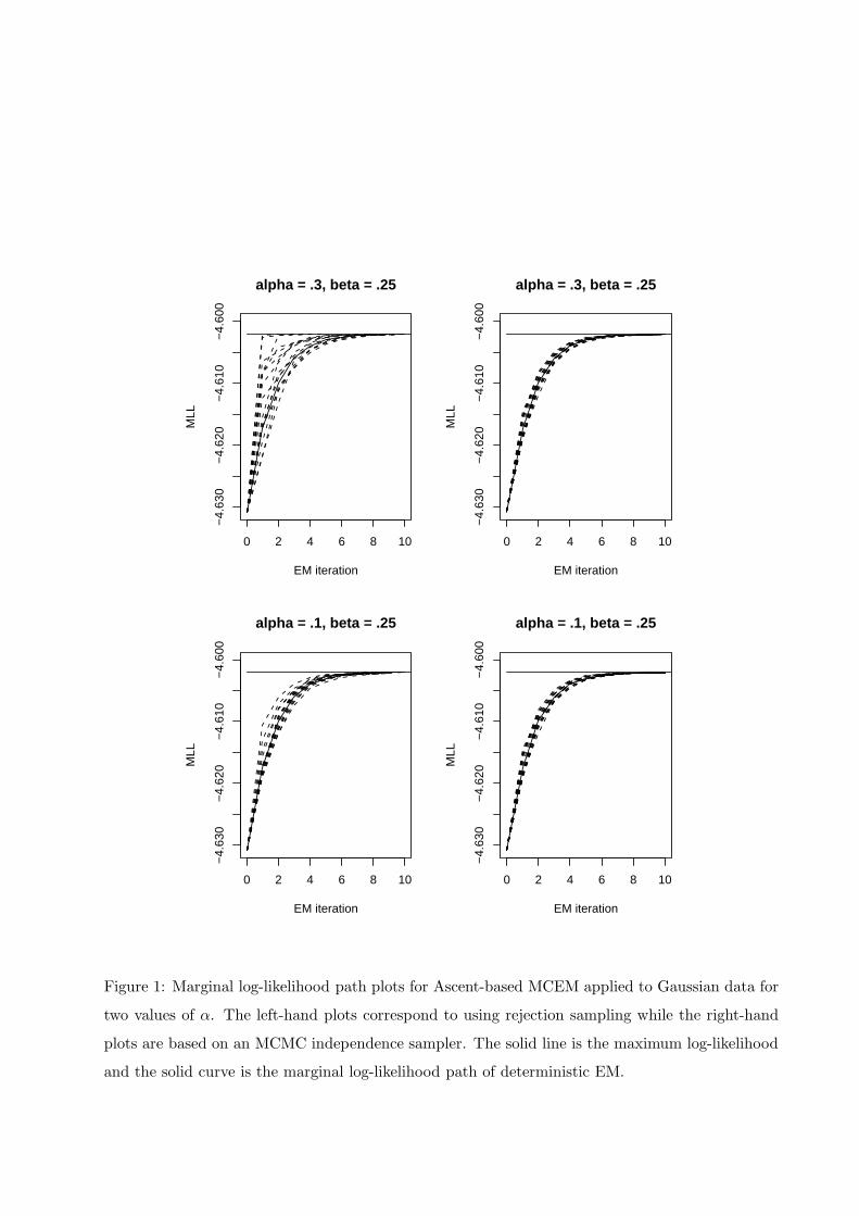
with n = 5 and λ = 1. The mle is λ = 1.3183. Consider the bottom two plots in Figure 1 (We will

return to this figure later.) which contain plots of the marginal log-likelihood paths for EM and 15

replications of Ascent-based MCEM under two sampling schemes: In the left-hand plot, we used

rejection sampling to draw a random sample from fU |Y (u|y; λ(t−1)) while, in the right-hand plot,

we used a Metropolis-Hastings independence sampler having invariant density fU |Y (u|y; λ(t−1)) and

a Normal(0, λ(t−1)) candidate density. We started all three algorithms at 1, i.e., λ(0) = λ(0) = 1.

Figure 1 indicates that, at least in this example, Ascent-based MCEM mimics EM well and appears

to recover the ascent property.

The rest of the article is organized as follows. Ascent-based MCEM is developed in Section 2.

In Section 3 we examine the performance of Ascent-based MCEM in several examples.

5

2 ASCENT-BASED MONTE CARLO EM

2.1 Recovering the Ascent Property

Recall that λ(t−1) denotes the current MCEM parameter estimate and that {u(t,j)}mt

j=1 is the Monte

Carlo sample. Let λ(t,mt) be the corresponding maximizer of Q(λ, λ(t−1)). Since an increase in the

Q-function implies the ascent property, we will check (4) by checking (3). That is, the algorithm

requires evidence that

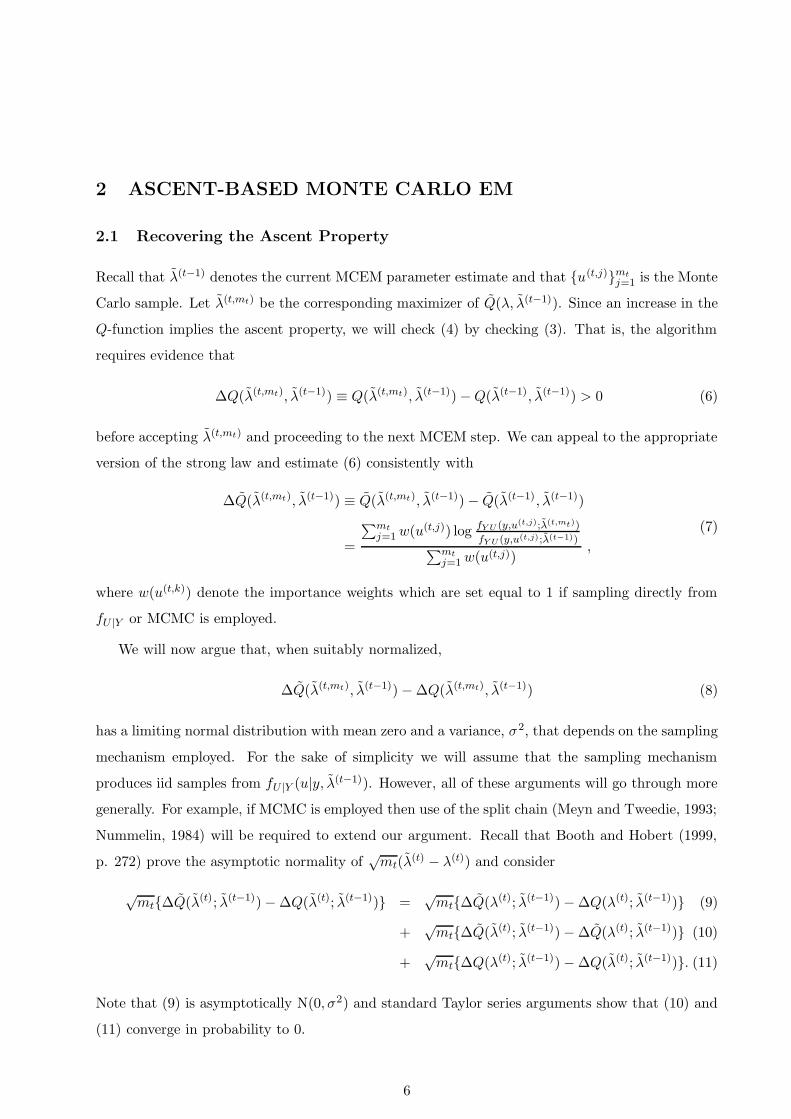
∆Q(λ(t,mt), λ(t−1)) ≡ Q(λ(t,mt), λ(t−1)) − Q(λ(t−1), λ(t−1)) > 0 (6)

before accepting λ(t,mt) and proceeding to the next MCEM step. We can appeal to the appropriate

version of the strong law and estimate (6) consistently with

∆Q(λ(t,mt), λ(t−1)) ≡ Q(λ(t,mt), λ(t−1)) − Q(λ(t−1), λ(t−1))

=

∑mt

j=1 w(u(t,j)) log fY U (y,u(t,j);λ(t,mt))

fY U (y,u(t,j);λ(t−1))∑mt

j=1 w(u(t,j)),

(7)

where w(u(t,k)) denote the importance weights which are set equal to 1 if sampling directly from

fU |Y or MCMC is employed.

We will now argue that, when suitably normalized,

∆Q(λ(t,mt), λ(t−1)) − ∆Q(λ(t,mt), λ(t−1)) (8)

has a limiting normal distribution with mean zero and a variance, σ2, that depends on the sampling

mechanism employed. For the sake of simplicity we will assume that the sampling mechanism

produces iid samples from fU |Y (u|y, λ(t−1)). However, all of these arguments will go through more

generally. For example, if MCMC is employed then use of the split chain (Meyn and Tweedie, 1993;

Nummelin, 1984) will be required to extend our argument. Recall that Booth and Hobert (1999,

p. 272) prove the asymptotic normality of√

mt(λ(t) − λ(t)) and consider

√mt{∆Q(λ(t); λ(t−1)) − ∆Q(λ(t); λ(t−1))} =

√mt{∆Q(λ(t); λ(t−1)) − ∆Q(λ(t); λ(t−1))} (9)

+√

mt{∆Q(λ(t); λ(t−1)) − ∆Q(λ(t); λ(t−1))} (10)

+√

mt{∆Q(λ(t); λ(t−1)) − ∆Q(λ(t); λ(t−1))}. (11)

Note that (9) is asymptotically N(0, σ2) and standard Taylor series arguments show that (10) and

(11) converge in probability to 0.

6

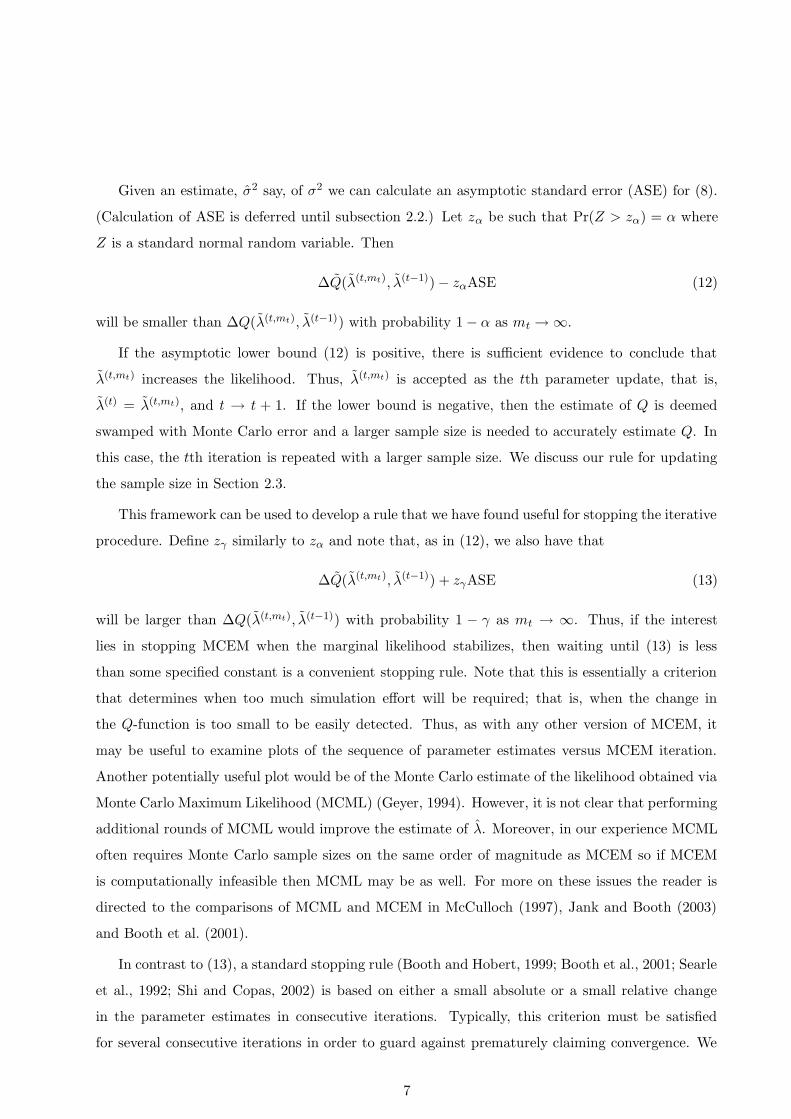
Given an estimate, σ2 say, of σ2 we can calculate an asymptotic standard error (ASE) for (8).

(Calculation of ASE is deferred until subsection 2.2.) Let zα be such that Pr(Z > zα) = α where

Z is a standard normal random variable. Then

∆Q(λ(t,mt), λ(t−1)) − zαASE (12)

will be smaller than ∆Q(λ(t,mt), λ(t−1)) with probability 1 − α as mt → ∞.

If the asymptotic lower bound (12) is positive, there is sufficient evidence to conclude that

λ(t,mt) increases the likelihood. Thus, λ(t,mt) is accepted as the tth parameter update, that is,

λ(t) = λ(t,mt), and t → t + 1. If the lower bound is negative, then the estimate of Q is deemed

swamped with Monte Carlo error and a larger sample size is needed to accurately estimate Q. In

this case, the tth iteration is repeated with a larger sample size. We discuss our rule for updating

the sample size in Section 2.3.

This framework can be used to develop a rule that we have found useful for stopping the iterative

procedure. Define zγ similarly to zα and note that, as in (12), we also have that

∆Q(λ(t,mt), λ(t−1)) + zγASE (13)

will be larger than ∆Q(λ(t,mt), λ(t−1)) with probability 1 − γ as mt → ∞. Thus, if the interest

lies in stopping MCEM when the marginal likelihood stabilizes, then waiting until (13) is less

than some specified constant is a convenient stopping rule. Note that this is essentially a criterion

that determines when too much simulation effort will be required; that is, when the change in

the Q-function is too small to be easily detected. Thus, as with any other version of MCEM, it

may be useful to examine plots of the sequence of parameter estimates versus MCEM iteration.

Another potentially useful plot would be of the Monte Carlo estimate of the likelihood obtained via

Monte Carlo Maximum Likelihood (MCML) (Geyer, 1994). However, it is not clear that performing

additional rounds of MCML would improve the estimate of λ. Moreover, in our experience MCML

often requires Monte Carlo sample sizes on the same order of magnitude as MCEM so if MCEM

is computationally infeasible then MCML may be as well. For more on these issues the reader is

directed to the comparisons of MCML and MCEM in McCulloch (1997), Jank and Booth (2003)

and Booth et al. (2001).

In contrast to (13), a standard stopping rule (Booth and Hobert, 1999; Booth et al., 2001; Searle

et al., 1992; Shi and Copas, 2002) is based on either a small absolute or a small relative change

in the parameter estimates in consecutive iterations. Typically, this criterion must be satisfied

for several consecutive iterations in order to guard against prematurely claiming convergence. We

7

believe this approach is understandable but somewhat misguided since it places the emphasis on the

behavior of the parameter estimates with little or no regard to the estimation of the information.

We address this issue in the context of a benchmark example in Section 3.1.

2.2 Monte Carlo Standard Errors

2.2.1 Independent Sampling

If importance sampling is employed an estimate of σ2 is given by

σ2 = mt

(

∑

w(u(t,j))Λ(u(t,j))∑

w(u(t,j))

)2(∑[

w(u(t,j))Λ(u(t,j))]2

[∑

w(u(t,j))Λ(u(t,j))]2 − 2

∑

w2(u(t,j))Λ(u(t,j))[∑

w(u(t,j))Λ(u(t,j))] [∑

w(u(t,j))]

+

∑

w2(u(t,j))[∑

w(u(t,j))]2

)

(14)

where the sums all range from j = 1, . . . ,mt and

Λ(u(t,j)) = logfY U (y, u(t,j); λ(t,mt))

fY U (y, u(t,j); λ(t−1)).

This is a standard formula for the variance of the ratio of two means (Kendall and Stuart, 1958, p.

232) applied to the importance sampling ratio estimator . With rejection sampling the importance

weights are set to 1 and (14) reduces to the (biased) sample variance of the mt independent terms

Λ(u(t,j)). Thus, in either case, it is easy to estimate ASE with σ/√

mt.

2.2.2 Markov Chain Monte Carlo

Calculating a reasonable Monte Carlo standard error is more difficult when we are forced to employ

MCMC. There are several different methods for doing this, including regenerative simulation (RS)

and batch means. Here we investigate the use of RS instead of batch means since it produces a

strongly consistent estimate of σ2 under weaker regularity conditions (Jones et al., 2004). However,

there are settings where a method such as batch means will be preferred.

We will give only a sketch of our implementation of RS as the details have appeared elsewhere;

see e.g., Hobert et al. (2002); Jones et al. (2004); Jones and Hobert (2001); and Mykland et al.

(1995). The basic idea is that one simulates a Markov chain in such a way that it is possible to

identify regeneration times that break the chain into tours that are iid.

Assume that the simulation is started with a regeneration (this is often easy to do, see Mykland

et al. (1995) for some examples) and hence we do not require any burn-in. Let 0 = τ0 < τ1 < τ2 <

8

· · · be the regeneration times and suppose that the simulation is run for a fixed number, Rt, of

tours. Then the total length of the simulation τRt is random. Let Nr = τr − τr−1 and define

Sr(λ, λ(t−1)) =

τr−1∑

j=τr−1

logfY U (y, u(t,j);λ)

fY U (y, u(t,j); λ(t−1)).

The (Sr(λ, λ(t−1)), Nr), r = 1, . . . , Rt pairs are iid since each is based on a different tour.

Now, under regularity conditions (Jones et al., 2004), a consistent estimate of the desired

asymptotic variance is given by

γ2(λ, λ(t−1)) =

∑Rt

r=1

{

Sr(λ, λ(t−1)) − S(λ,λ(t−1))N

Nr

}2

RtN2.

Since λ(t) is unknown, we estimate the ASE with γ(λ(t,τRt), λ(t−1))/

√Rt, where λ(t,τRt

) denotes the

maximizer of (5) based on Rt regenerations of the chain. Therefore, an asymptotic lower bound

for (7) is given by

∆Q(λ(t,τRt), λ(t−1)) − zα

γ(λ(t,τRt), λ(t−1))√Rt

.

2.3 Updating the Monte Carlo Sample Size

Because the initial jumps in the EM algorithm are typically large, it has become conventional

wisdom that smaller Monte Carlo sample sizes can be tolerated in the initial stages of MCEM.

However, larger sample sizes will be required later in order to decrease the variability of λ(t).

Therefore, we need a rule for increasing the sample size as the computation progresses.

To motivate our solution we digress and briefly consider a general MCEM algorithm; that is, not

necessarily Ascent-based MCEM. The probability that the ascent property does not hold between

two consecutive iterations is Pr{Q(λ(t), λ(t−1)) ≤ Q(λ(t−1), λ(t−1))}. Note that this probability does

not correspond to α from (12) and if mt → ∞ then Pr{Q(λ(t), λ(t−1)) ≤ Q(λ(t−1), λ(t−1))} → 0.

Thus, regardless of the initial Monte Carlo sample size, by increasing the sample size within an

E-Step the algorithm will reach a point where the ascent property very likely holds.

Another interesting observation follows if we assume that the Monte Carlo sample sizes are

increased between MCEM steps fast enough so that

∞∑

t=1

Pr{Q(λ(t), λ(t−1)) ≤ Q(λ(t−1), λ(t−1))} < ∞ .

Then Borel-Cantelli (Billingsley, 1995, pp 59-60) says that, with probability 1, the sequence {λ(t)}has the ascent property except for perhaps finitely many iterations. Therefore, this realization of

9

an MCEM algorithm defines an eventual (i.e., for all MCEM iterations, t > N , where N < ∞)

realization of a deterministic GEM algorithm.

We now return to Ascent-based MCEM. Recall that the current Monte Carlo sample size, mt, is

repeatedly increased within the tth MCEM step until the asymptotic lower bound (12) is positive.

We propose a geometric rate of increase; specifically, we set the next Monte Carlo sample size to

be mt + mt/k for some k = 2, 3, . . .. The mt/k additional samples are drawn and appended to the

current sample. This process clearly trades computing time for stability. However, for automated

algorithms, we believe that computing time is less of a concern than confidence in the output of

the algorithm. On a related note, it is possible to use an importance weighting scheme and use

samples from all of the previous simulations as in Booth and Hobert (1999) and Quintana et al.

(1999). However, authors such as Booth and Hobert (1999) find little advantage in this approach

and in our experience with Ascent-based MCEM it often requires an enormous amount of storage

and hence negatively impacts computational efficiency.

In the interest of obtaining computational efficiency and avoiding severe inflation of the type 1

error rate the starting sample size for each MCEM iteration should be chosen so that we go through

the appending process infrequently. For MCEM iteration t, let mt,start be the starting Monte Carlo

sample size and mt,end be the ending Monte Carlo sample size. In order to force an increase (on

average) in the Monte Carlo sample sizes across MCEM iterations we take mt+1,start ≥ mt,start. If

we assume that

∆Q(λ(t+1), λ(t)) ∼ N

(

∆Q(λ(t+1), λ(t)),σ2

mt+1

)

then we can use standard sample size calculations to determine the value of mt+1,start. In particular,

under independent sampling we set

mt+1,start = max{

mt,start, σ2(zα + zβ)2/[∆Q(λ(t), λ(t−1))]2}

, (15)

where β is a specified type 2 error rate and σ2 is an estimate of the variance of ∆Q developed

in Section 2.2. Since ∆Q(λ(t+1), λ(t)) depends on unknown quantities we have replaced it with an

estimate from the previous iteration. Recall that under RS we do not choose the Monte Carlo

sample size but instead we fix the number of regenerations, Rt. Since these Rt tours are iid the

above sample size calculation is applied to the number of regenerations.

The validity of (15) clearly relies on the quality of the normal approximation. A poor approxi-

mation primarily results in an inflated type 1 error rate for the lower bound. To illustrate the effect

of inflating α we took the setting of Example 1 and performed Ascent-based MCEM for 2 levels

of α and both sampling mechanisms. The results are given in Figure 1. The plots indicate that,

10

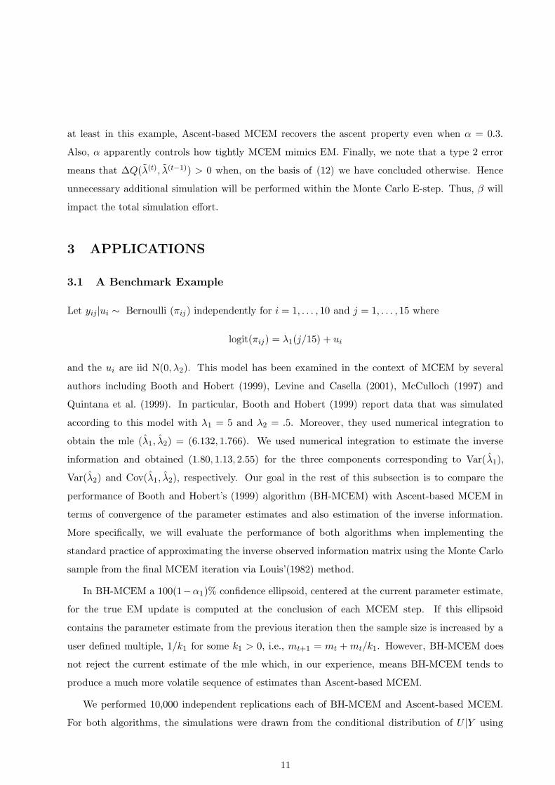
at least in this example, Ascent-based MCEM recovers the ascent property even when α = 0.3.

Also, α apparently controls how tightly MCEM mimics EM. Finally, we note that a type 2 error

means that ∆Q(λ(t), λ(t−1)) > 0 when, on the basis of (12) we have concluded otherwise. Hence

unnecessary additional simulation will be performed within the Monte Carlo E-step. Thus, β will

impact the total simulation effort.

3 APPLICATIONS

3.1 A Benchmark Example

Let yij|ui ∼ Bernoulli (πij) independently for i = 1, . . . , 10 and j = 1, . . . , 15 where

logit(πij) = λ1(j/15) + ui

and the ui are iid N(0, λ2). This model has been examined in the context of MCEM by several

authors including Booth and Hobert (1999), Levine and Casella (2001), McCulloch (1997) and

Quintana et al. (1999). In particular, Booth and Hobert (1999) report data that was simulated

according to this model with λ1 = 5 and λ2 = .5. Moreover, they used numerical integration to

obtain the mle (λ1, λ2) = (6.132, 1.766). We used numerical integration to estimate the inverse

information and obtained (1.80, 1.13, 2.55) for the three components corresponding to Var(λ1),

Var(λ2) and Cov(λ1, λ2), respectively. Our goal in the rest of this subsection is to compare the

performance of Booth and Hobert’s (1999) algorithm (BH-MCEM) with Ascent-based MCEM in

terms of convergence of the parameter estimates and also estimation of the inverse information.

More specifically, we will evaluate the performance of both algorithms when implementing the

standard practice of approximating the inverse observed information matrix using the Monte Carlo

sample from the final MCEM iteration via Louis’(1982) method.

In BH-MCEM a 100(1−α1)% confidence ellipsoid, centered at the current parameter estimate,

for the true EM update is computed at the conclusion of each MCEM step. If this ellipsoid

contains the parameter estimate from the previous iteration then the sample size is increased by a

user defined multiple, 1/k1 for some k1 > 0, i.e., mt+1 = mt + mt/k1. However, BH-MCEM does

not reject the current estimate of the mle which, in our experience, means BH-MCEM tends to

produce a much more volatile sequence of estimates than Ascent-based MCEM.

We performed 10,000 independent replications each of BH-MCEM and Ascent-based MCEM.

For both algorithms, the simulations were drawn from the conditional distribution of U |Y using

11

an accept-reject sampler. Each replication was started at (λ(0)1 , λ

(0)2 ) = (0, 1) and the initial sample

size was m0 = 10. Each replication was terminated when the relative change in two successive

parameter updates was less than 2% for C ≥ 1 consecutive MCEM steps where C = 1 for Ascent-

based MCEM and C = 1, 2, 3, 4 for BH-MCEM. With Ascent-based MCEM we used α = 0.25,

β = .25 and set k = 3 while for BH-MCEM we used α1 = 0.25 and k1 = 3.

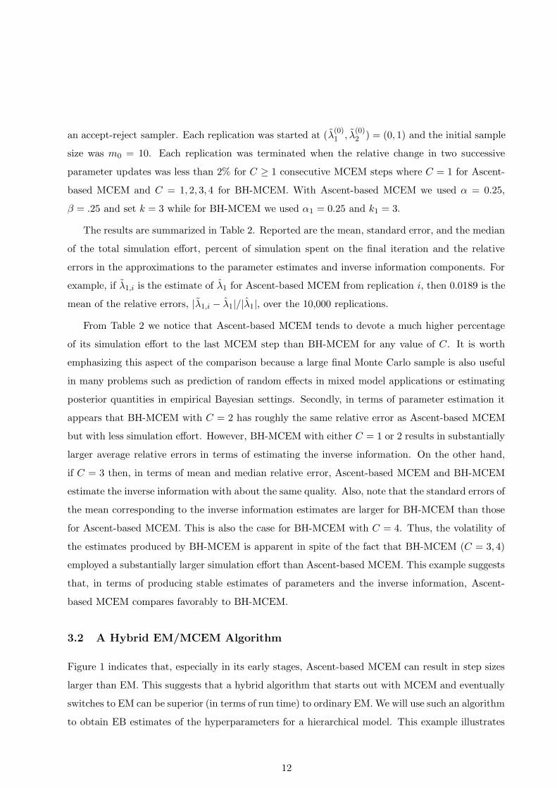
The results are summarized in Table 2. Reported are the mean, standard error, and the median

of the total simulation effort, percent of simulation spent on the final iteration and the relative

errors in the approximations to the parameter estimates and inverse information components. For

example, if λ1,i is the estimate of λ1 for Ascent-based MCEM from replication i, then 0.0189 is the

mean of the relative errors, |λ1,i − λ1|/|λ1|, over the 10,000 replications.

From Table 2 we notice that Ascent-based MCEM tends to devote a much higher percentage

of its simulation effort to the last MCEM step than BH-MCEM for any value of C. It is worth

emphasizing this aspect of the comparison because a large final Monte Carlo sample is also useful

in many problems such as prediction of random effects in mixed model applications or estimating

posterior quantities in empirical Bayesian settings. Secondly, in terms of parameter estimation it

appears that BH-MCEM with C = 2 has roughly the same relative error as Ascent-based MCEM

but with less simulation effort. However, BH-MCEM with either C = 1 or 2 results in substantially

larger average relative errors in terms of estimating the inverse information. On the other hand,

if C = 3 then, in terms of mean and median relative error, Ascent-based MCEM and BH-MCEM

estimate the inverse information with about the same quality. Also, note that the standard errors of

the mean corresponding to the inverse information estimates are larger for BH-MCEM than those

for Ascent-based MCEM. This is also the case for BH-MCEM with C = 4. Thus, the volatility of

the estimates produced by BH-MCEM is apparent in spite of the fact that BH-MCEM (C = 3, 4)

employed a substantially larger simulation effort than Ascent-based MCEM. This example suggests

that, in terms of producing stable estimates of parameters and the inverse information, Ascent-

based MCEM compares favorably to BH-MCEM.

3.2 A Hybrid EM/MCEM Algorithm

Figure 1 indicates that, especially in its early stages, Ascent-based MCEM can result in step sizes

larger than EM. This suggests that a hybrid algorithm that starts out with MCEM and eventually

switches to EM can be superior (in terms of run time) to ordinary EM. We will use such an algorithm

to obtain EB estimates of the hyperparameters for a hierarchical model. This example illustrates

12

how the judicious use of Ascent-based MCEM can accelerate the convergence of deterministic EM.

This example is motivated by a microarray experiment which attempted to identify genes that

behave differently across tissue types for subjects with varying ages. In particular, levels of “expres-

sion” for several genes were measured across experimental conditions hoping to locate candidate

genes that are differentially expressed across tissue types and ages.

Let Yi be a vector of J responses for i = 1, . . . , n. Here, i represents the gene index and n

represents the number of genes (n may be on the order of ten to twenty thousand in microarray

experiments). Let x be a J × p matrix of covariates (e.g., tissue type and subject age). Suppose

that conditional on u1i, u2i the data, Yi, are independent with

Yi|u1i, u2i ∼ Normal(xu1i, Iu−12i ),

where I is an identity matrix. At the second stage, conditional on u2i the U1i are independent with

U1i|u2i ∼ Normal(0, λ1u−12i ),

where each u1i is a p× 1 vector and λ1 is a p× p matrix. Finally, the U2i are assumed independent

with

U2i ∼ Gamma(λ2, λ3),

where λ2 is the Gamma shape parameter and λ3 is the Gamma rate parameter (then the Gamma

mean is λ2/λ3). Note that U1i may be viewed as the gene-specific random mean while U2i is the

gene-specific random precision. Throughout we assume that λ1, λ2 and λ3 are strictly positive so

that the priors are all proper. The EB estimate of λ = (λ1, λ2, λ3)T maximizes (1), where y is the

observed data and U contains the U1i and U2i. Therefore, EM may be used to calculate the EB

estimate of λ.

A convenient feature of EM is that λ(t)1 has closed form and can be calculated independently

of λ(t)2 and λ

(t)3 . However, EM is computationally burdensome in this setting since at least one

complete pass through the gene index, i, is required at each EM iteration. This burden may be

lessened by using MCEM. The basic idea is to sum over only a random subset of the gene index in

the early stages of the hybrid algorithm. When the Monte Carlo sample sizes for MCEM get too

large, the algorithm then switches to EM.

The Q-function (up to a scalar constant) is given by

Q(λ, λ(t−1)) =1

n

n∑

i=1

E{log fY,U(yi, U1i, U2i;λ) | yi, λ(t−1)}. (16)

13

Let U3 be uniformly distributed on the integers 1, . . . , n, independently of y. Using U3, we can

rewrite (16) as

Q(λ, λ(t−1)) = E{log fY,U(yU3 , U1U3 , U2U3 ;λ) | y, λ(t−1)}, (17)

where, for example, the notation yU3 refers to the vector yi with i evaluated at the random index

U3. It is easy to sample directly from fU |Y via sequential sampling as we now describe.

Let shape(i) and rate(i) be the shape and rate parameters for the Gamma density of U2i|yi, λ(t−1).

Similarly, let mean(i, u2i) and var(i, u2i) be the mean and variance corresponding to the Normal

density of U1i|u2i, yi, λ(t−1). Formulas for these quantities are given in Table 3. The sequential

sampling mechanism for generating from fU |Y follows:

1. simulate u(t,j)3 uniformly on the integers 1, . . . , n,

2. simulate u(t,j)2 as Gamma{shape(u

(t,j)3 ), rate(u

(t,j)3 )},

3. simulate u(t,j)1 as Normal{mean(u

(t,j)3 , u

(t,j)2 ), var(u

(t,j)3 , u

(t,j)2 )}.

With these simulated variables it is easy to form a Monte Carlo approximation to (17).

The algorithm proceeds by using our MCEM algorithm in the early stages and then in the later

stages EM based on (16). A rough estimate of the computational effort, obtained by inspecting

the program code, suggests that at least 2mt nontrivial computations are required for one MCEM

iteration. In contrast, one EM iteration needs n nontrivial computations. Therefore, we switch

from MCEM to EM when the ending Monte Carlo sample size for the current MCEM iteration is

larger than n/2. Finally, notice that this hybrid algorithm does not require a stochastic stopping

criterion since EM is used in the final stages of the algorithm.

3.2.1 A Numerical Example

We simulated data from the assumed hierarchical model for n = 20, 000, n = 60, 000 and n =

100, 000 with λ1, λ2 and x (20×5) obtained from a specific microarray experiment. The simulated

data are available upon request.

We set λ(0)1 equal to the identity matrix, λ

(0)2 = λ

(0)3 = 1, α = 0.3, β = 0.05, k = 2 and performed

100 independent runs of the hybrid algorithm. This was repeated for each of the 3 values of n.

We also ran an EM algorithm using the same starting values. All programs were run on the same

computer and the same code was used for both EM and the EM portion of the hybrid algorithm.

14

The run times for the hybrid algorithm were substantially better than those for EM. In par-

ticular, when n = 20, 000, it took EM 6 minutes and 17 seconds (6:17) to converge. On the other

hand, the maximum run time for the hybrid algorithm was 4:56; an improvement of 22%. The

minimum, 25th, 50th and 75th percentiles of the run times for the hybrid algorithm are 1:29, 3:24,

3:47, and 4:13 respectively. This clearly indicates that the hybrid algorithm performs much better

than deterministic EM in this example. Moreover, the improvement in run time can be even more

substantial as n increases. For example, with n = 60, 000 the five number summary for the run

times for the hybrid algorithm was (3:25, 8:55, 9:44, 11:00, 13:23) while EM took 18:60. That is,

the improvement ranged from 30% to 82%. When n = 100, 000 the five number summary of the

run times for the hybrid algorithm was (5:35, 13:21, 15:27, 16:42, 21:20) and EM required 31:46.

There is one important caveat to our results: The hybrid algorithm may be less efficient than EM

if the starting values are chosen very close to the (unknown) mle.

3.3 Empirical Bayes Estimates for a Hierarchical Model

3.3.1 The Model and Gibbs Sampler

Suppose that conditional on θ = (θ1, . . . , θA)T and νe, the data, Yij, are independent with

Yij |θi, νe ∼ Normal(θi, ν−1e )

where i = 1, . . . , A and j = 1, . . . , ni. At the second stage, conditional on µ and νθ, θ1, . . . , θA and

νe are independent with

θi|µ, νθ ∼ Normal(µ, ν−1θ ) and νe ∼ Gamma(a2, λ2).

Finally, at the third stage, µ and νθ are assumed independent with

µ ∼ Normal(µ0, ν−10 ) and νθ ∼ Gamma(a1, λ1)

where µ0, ν0, a1, λ1, a2, λ2 are constants and all but µ0 are assumed to be strictly positive; hence

all of the priors are proper. Regardless of the prior specification on the variance components, the

EB estimate of µ0 is the overall mean, y =∑

ij yij/n where n =∑

i ni. Also, for reasons discussed

in Subsection 3.3.2, we focus on estimating λ1 and λ2 for fixed a1, a2 and ν0.

Note that, in terms of the EM notation, we have U = (θ, µ, νθ, νe)T , and λ = (λ1, λ2)

T . Then

the Q-function is an expectation with respect to the posterior density. Thus, a consequence of

MCEM is that the final Monte Carlo sample used to approximate the Q-function is a sample from

15

the posterior required for EB inference. We will use the block Gibbs sampler, introduced by Hobert

and Geyer (1998), to sample (approximately) from the posterior.

3.3.2 A Numerical Example

Littell et al. (1996, p.141) give data arising from an experiment in which six randomly chosen

influents for the Mississippi River are used to monitor the nitrogen concentration in parts per

million.

The EB estimate of µ0 is y and of the remaining parameters we choose to estimate only λ1 and

λ2. One reason for this choice is that the EB estimate of ν0 is ∞. That is, the EB estimate of the

prior on µ is a point mass at the overall mean. Therefore, we fix ν0 at an a priori specified value; in

this example we chose 0.1. Furthermore, maximizing the posterior with respect to all of a1, λ1, and

a2, λ2 is unstable, since it is flat in the direction of fixed means, a1/λ1 and a2/λ2. Therefore, we

chose to fix the prior variances, a1/λ21 and a2/λ

22, at 0.1, which leaves only λ1 and λ2 identifiable.

For starting values we used a method of moments approach. Specifically, we set the prior

expectations for νθ and νe equal to the obvious values

E(νθ) =a1

λ1=

n

MSTR − MSE= 0.108 and E(νe) =

a2

λ2=

1

MSE= 0.0235

and solved for a1, λ1, a2, and λ2. This yields a1 = 1.17, λ1 = 1.08, a2 = 0.006 and λ2 = 0.235.

We will retain the values for a1 and a2 and use the estimates of λ1 and λ2 as starting values in our

MCEM program, that is, λ(0) = (1.08, 0.235)T .

For the MCEM algorithm we set k = 2, α = 0.3 and β = 0.25. In each MCEM step the

starting value for the block Gibbs sampler was (y1, y2, . . . , y6, y)T . The use of RS in this setting

was described in Jones and Hobert (2001). We set γ = 0.05 and declared convergence when (13)

fell below 10−5. The computation terminated after 8 MCEM iterations. The EB estimates are

λ(8) = (59.618, 0.258)T . Table 4 reports the number of regenerations and the average number of

iterations of the block Gibbs sampler per regeneration for each MCEM step. The initial number of

regenerations was specified to be 5.

3.4 An Application to Model-Based Spatial Statistics

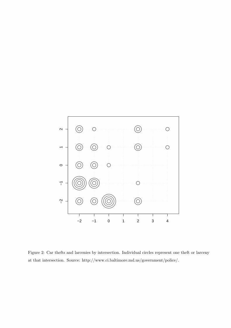
Figure 2 depicts counts of auto thefts and larcenies for a grid of city streets in southeast Baltimore

over a period of 70 days. Each individual circle in the figure represents an auto theft or a larceny

at or near that intersection. While it is reasonable to model these counts as realizations of Poisson

16

random variables, assuming independence for counts in close geographical proximity is not. Thus,

we propose a generalized linear mixed model (GLMM) that uses the random effects to account for

the spatial correlation (Diggle et al., 1998). Note that fitting this model involves approximating an

intractable integral whose dimension is the total number of responses.

Let xi, i = 1, . . . , n, be bivariate data points representing the locations of the 35 observed

intersections, and let yi denote the number of auto thefts and larcenies at intersection xi. Let

U = (U1, . . . , Un)T be a vector of random effects. Conditional on u, we assume that yi follows a

Poisson density with mean µi satisfying

log(µi) = λ1 + ui. (18)

Finally, we assume that U follows a multivariate normal distribution with mean zero and variance-

covariance matrix, Σ, whose i, j element is given by

Σij = λ2 exp{−λ3‖xi − xj‖} . (19)

That is, the correlation between any two random effects decays exponentially with the geographic

distance between the associated observations.

Unlike applications of GLMMs with subject or strata level random effects, the marginal likeli-

hood does not factor into the product of several smaller dimensional integrals. Therefore, numerical

integration is not an option, even for relatively small values of n. The same problem occurs with

the integrals required for performing EM. However, fitting via the EM algorithm is appealing in

this setting because considerable simplifications occur in the log of the complete data likelihood.

Unfortunately, direct simulation from fU |Y (u|y;λ(t−1)) is not possible. We will investigate the

use of two different sampling mechanisms; the Esup rejection sampler proposed by Caffo et al. (2002)

and importance sampling both using a candidate density obtained by shifting and scaling student’s

t density by the Laplace approximation to the mean and standard deviation of the distribution of

U |y;λ(t−1). The formulas for these approximations are given in Appendix A.

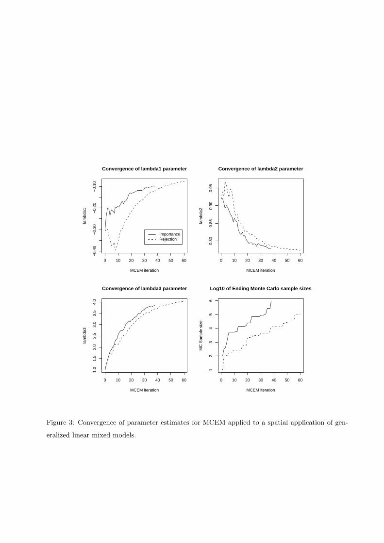
Figure 3 shows the path plots of the parameter estimates and the Monte Carlo sample sizes

for the two versions of our algorithm. We set α = .15, β = .3 and k = 2. The starting values

λ(0) = (−.3, .92, 1)T were obtained as the posterior modes from the R (Ihaka and Gentleman,

1996) contributed software package geoRglm (Christensen and Ribeiro Jr, 2002) for a fixed value

of λ3 = 1. The algorithm converged in 56 MCEM steps for rejection sampling and 44 MCEM

steps for importance sampling. We set γ = 0.05 and declared convergence when (13) fell below

17

10−4. The final estimates were λ(44) = (−.087, .776, 4.00)T for importance sampling and λ(56) =

(−.082, .775, 3.99)T for rejection sampling. The computing time for both algorithms was similar.

A Laplace Approximation for Section 3.4

The Laplace approximation, µ∗, to E(U |y; λ(t−1)) is the solution to

∂

∂ulog fY U (y, u;λ(t−1)) = y − µ − Σ−1u = 0

where µ = exp(λ(t−1)1 + u) and Σ is the variance covariance matrix defined by (19) evaluated at

λ(t−1)2 and λ

(t−1)3 . The Laplace approximation to Var(U |y; λ(t−1)) is

{

∂2

∂u∂uTlog fY U (y, u;λ(t−1))

}−1

={

Diag(µ∗) + Σ−1}−1

where Diag(µ∗) is a diagonal matrix with µ∗ along the main diagonal.

Acknowledgments. The authors are grateful to Jim Booth, Charlie Geyer, Jim Hobert and

Tom Louis for many helpful comments and suggestions.

References

Billingsley, P. (1995). Probability and Measure. Wiley, New York, third edition.

Booth, J. G. and Hobert, J. P. (1999). Maximizing generalized linear mixed model likelihoods with

an automated Monte Carlo EM algorithm. Journal of the Royal Statistical Society, Series B,

61:265–285.

Booth, J. G., Hobert, J. P., and Jank, W. S. (2001). A survey of Monte Carlo algorithms for

maximizing the likelihood of a two-stage hierarchical model. Statistical Modelling, 1:333–349.

Caffo, B. S., Booth, J. G., and Davison, A. C. (2002). Empirical sup rejection sampling. Biometrika,

89:745–754.

Christensen, O. F. and Ribeiro Jr, P. J. (2002). geoRglm - a package for generalised linear spatial

models. R News, 2:26–28.

Dempster, A. P., Laird, N. M., and Rubin, D. B. (1977). Maximum likelihood from incomplete

data via the EM algorithm. Journal of the Royal Statistical Society, Series B, 39:1–22.

18

Diggle, P. J., Tawn, J. A., and Moyeed, R. A. (1998). Model-based geostatistics (with discussion).

Applied Statistics, 47:299–326.

Geyer, C. J. (1994). On the convergence of Monte Carlo maximum likelihood calculations. Journal

of the Royal Statistical Society, Series B, 56:261–274.

Gueorguieva, R. and Agresti, A. (2001). A correlated probit model for joint modeling of clustered

binary and continuous responses. Journal of the American Statistical Association, 96:1102–1112.

Hobert, J. P. and Geyer, C. J. (1998). Geometric ergodicity of Gibbs and block Gibbs samplers for

a hierarchical random effects model. Journal of Multivariate Analysis, 67:414–430.

Hobert, J. P., Jones, G. L., Presnell, B., and Rosenthal, J. S. (2002). On the applicability of

regenerative simulation in Markov chain Monte Carlo. Biometrika, 89:731–743.

Ihaka, R. and Gentleman, R. (1996). R: A language for data analysis and graphics. Journal of

Computational and Graphical Statistics, 5:299–314.

Jank, W. and Booth, J. G. (2003). Efficiency of Monte Carlo EM and simulated maximum likelihood

in two-stage hierarchical models. Journal of Computational and Graphical Statistics, 12:214–229.

Jones, G. L., Haran, M., and Caffo, B. S. (2004). Output analysis for Markov chain Monte Carlo

simulations. Technical report, University of Minnesota, School of Statistics.

Jones, G. L. and Hobert, J. P. (2001). Honest exploration of intractable probability distributions

via Markov chain Monte Carlo. Statistical Science, 16:312–334.

Kendall, M. G. and Stuart, A. (1958). The Advanced Theory of Statistics, volume 1. Charles Griffen

& Company Limited, London.

Lange, K. (1999). Numerical Analysis for Statisticians. Springer–Verlag, New York.

Levine, R. A. and Casella, G. (2001). Implementations of the Monte Carlo EM algorithm. Journal

of Computational and Graphical Statistics, 10:422–439.

Littell, R. C., Milliken, G. A., Stroup, W. W., and Wolfinger, R. D. (1996). SAS system for Mixed

Models. SAS Institute Inc., Cary, NC.

Louis, T. A. (1982). Finding the Observed Information Matrix when using the EM algorithm.

Journal of the Royal Statistical Society, Series B, 44:226–233.

19

McCulloch, C. E. (1994). Maximum likelihood variance components estimation for binary data.

Journal of the American Statistical Association, 89:330–335.

McCulloch, C. E. (1997). Maximum likelihood algorithms for generalized linear mixed models.

Journal of the American Statistical Association, 92:162–170.

Meyn, S. P. and Tweedie, R. L. (1993). Markov Chains and Stochastic Stability. Springer-Verlag,

London.

Mykland, P., Tierney, L., and Yu, B. (1995). Regeneration in Markov chain samplers. Journal of

the American Statistical Association, 90:233–241.

Nummelin, E. (1984). General Irreducible Markov Chains and Non-negative Operators. Cambridge

University Press, London.

Polyak, B. T. and Juditsky, A. B. (1992). Acceleration of stochastic–approximation by averaging.

SIAM Journal on Control and Optimization, 30:838–855.

Quintana, F. A., Liu, J. S., and del Pino, G. E. (1999). Monte Carlo EM with importance reweight-

ing and its applications in random effects models. Computational Statistics and Data Analysis,

29:429–444.

Robert, C. P. and Casella, G. (1999). Monte Carlo Statistical Methods. Springer, New York.

Searle, S. R., Casella, G., and McCulloch, C. E. (1992). Variance Components. John Wiley and

Sons, New York.

Shi, J. Q. and Copas, J. (2002). Publication bias and meta-analysis for 2 × 2 tables: an average

Markov chain Monte Carlo EM algorithm. Journal of the Royal Statistical Society, Series B,

64:221–236.

Wei, G. C. G. and Tanner, M. A. (1990). A Monte Carlo implementation of the EM algorithm and

the poor man’s data augmentation algorithms. Journal of the American Statistical Association,

85:699–704.

Wu, C. F. J. (1983). On the convergence properties of the EM algorithm. The Annals of Statistics,

11:95–103.

20

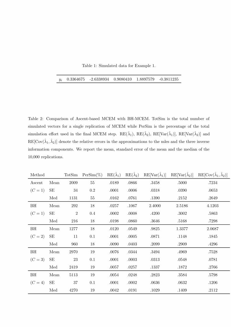
Table 1: Simulated data for Example 1.

yi 0.3364675 -2.6338934 0.9080410 1.8897579 -0.3811235

Table 2: Comparison of Ascent-based MCEM with BH-MCEM. TotSim is the total number of

simulated vectors for a single replication of MCEM while PerSim is the percentage of the total

simulation effort used in the final MCEM step. RE(λ1), RE(λ2), RE[Var(λ1)], RE[Var(λ2)] and

RE[Cov(λ1, λ2)] denote the relative errors in the approximations to the mles and the three inverse

information components. We report the mean, standard error of the mean and the median of the

10,000 replications.

Method TotSim PerSim(%) RE(λ1) RE(λ2) RE[Var(λ1)] RE[Var(λ2)] RE[Cov(λ1, λ2)]

Ascent Mean 2009 55 .0189 .0866 .3458 .5000 .7234

(C = 1) SE 34 0.2 .0001 .0006 .0318 .0390 .0653

Med 1131 55 .0162 .0761 .1390 .2152 .2649

BH Mean 292 18 .0257 .1067 2.4000 2.5186 4.1203

(C = 1) SE 2 0.4 .0002 .0008 .4200 .3002 .5863

Med 216 18 .0198 .0860 .3646 .5168 .7298

BH Mean 1277 18 .0120 .0549 .9825 1.3377 2.0687

(C = 2) SE 11 0.1 .0001 .0005 .0871 .1148 .1845

Med 960 18 .0090 .0403 .2099 .2909 .4296

BH Mean 2970 19 .0076 .0344 .3494 .4969 .7528

(C = 3) SE 23 0.1 .0001 .0003 .0313 .0548 .0781

Med 2419 19 .0057 .0257 .1337 .1872 .2766

BH Mean 5113 19 .0054 .0248 .2823 .3584 .5798

(C = 4) SE 37 0.1 .0001 .0002 .0636 .0632 .1206

Med 4270 19 .0042 .0191 .1029 .1409 .2112

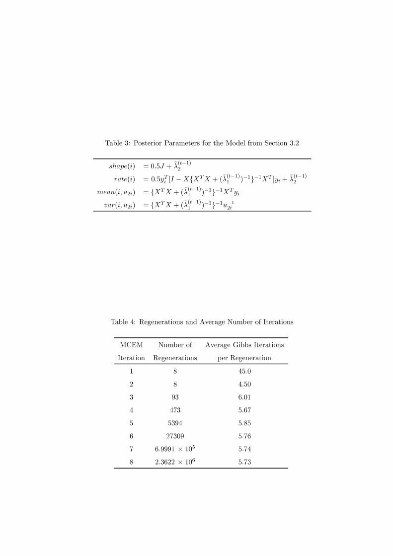
Table 3: Posterior Parameters for the Model from Section 3.2

shape(i) = 0.5J + λ(t−1)2

rate(i) = 0.5yTi [I − X{XT X + (λ

(t−1)1 )−1}−1XT ]yi + λ

(t−1)2

mean(i, u2i) = {XT X + (λ(t−1)1 )−1}−1XT yi

var(i, u2i) = {XT X + (λ(t−1)1 )−1}−1u−1

2i

Table 4: Regenerations and Average Number of Iterations

MCEM Number of Average Gibbs Iterations

Iteration Regenerations per Regeneration

1 8 45.0

2 8 4.50

3 93 6.01

4 473 5.67

5 5394 5.85

6 27309 5.76

7 6.9991 × 105 5.74

8 2.3622 × 106 5.73

0 2 4 6 8 10

−4.

630

−4.

620

−4.

610

−4.

600

EM iteration

MLL

alpha = .3, beta = .25

0 2 4 6 8 10

−4.

630

−4.

620

−4.

610

−4.

600

EM iteration

MLL

alpha = .1, beta = .25

0 2 4 6 8 10

−4.

630

−4.

620

−4.

610

−4.

600

EM iteration

MLL

alpha = .3, beta = .25

0 2 4 6 8 10

−4.

630

−4.

620

−4.

610

−4.

600

EM iteration

MLL

alpha = .1, beta = .25

Figure 1: Marginal log-likelihood path plots for Ascent-based MCEM applied to Gaussian data for

two values of α. The left-hand plots correspond to using rejection sampling while the right-hand

plots are based on an MCMC independence sampler. The solid line is the maximum log-likelihood

and the solid curve is the marginal log-likelihood path of deterministic EM.

−2 −1 0 1 2 3 4

−2

−1

01

2

Figure 2: Car thefts and larcenies by intersection. Individual circles represent one theft or larceny

at that intersection. Source: http://www.ci.baltimore.md.us/government/police/.

0 10 20 30 40 50 60

−0.

40−

0.30

−0.

20−

0.10

MCEM iteration

lam

bda1

Convergence of lambda1 parameter

ImportanceRejection

0 10 20 30 40 50 60

0.80

0.85

0.90

0.95

MCEM iteration

lam

bda2

Convergence of lambda2 parameter

0 10 20 30 40 50 60

1.0

1.5

2.0

2.5

3.0

3.5

4.0

MCEM iteration

lam

bda3

Convergence of lambda3 parameter

0 10 20 30 40 50 60

12

34

56

MCEM iteration

MC

Sam

ple

size

Log10 of Ending Monte Carlo sample sizes

Figure 3: Convergence of parameter estimates for MCEM applied to a spatial application of gen-

eralized linear mixed models.