asemigroupapproachtofinslergeometry: bakry–ledoux
TRANSCRIPT

arX
iv:1
602.
0039
0v3
[m
ath.
DG
] 2
9 A
ug 2
020
A semigroup approach to Finsler geometry:
Bakry–Ledoux’s isoperimetric inequality
Shin-ichi Ohta∗†‡
September 1, 2020
Abstract
We develop the celebrated semigroup approach a la Bakry et al on Finsler man-ifolds, where natural Laplacian and heat semigroup are nonlinear, based on theBochner–Weitzenbock formula established by Sturm and the author. We show theL1-gradient estimate on Finsler manifolds (under some additional assumptions inthe noncompact case), which is equivalent to a lower weighted Ricci curvature boundand the improved Bochner inequality. As a geometric application, we prove Bakry–Ledoux’s Gaussian isoperimetric inequality, again under some additional assump-tions in the noncompact case. This extends Cavalletti–Mondino’s inequality onreversible Finsler manifolds to non-reversible metrics, and improves the author’sprevious estimate, both based on the localization (also called needle decomposition)method.
Mathematics Subject Classification (2010): 53C60, 58J35, 49Q20
Contents
1 Introduction 2
2 Geometry and analysis on Finsler manifolds 4
2.1 Finsler manifolds . . . . . . . . . . . . . . . . . . . . . . . . . . . . . . . . . . . . 52.2 Uniform convexity and smoothness . . . . . . . . . . . . . . . . . . . . . . . . . . 72.3 Weighted Ricci curvature . . . . . . . . . . . . . . . . . . . . . . . . . . . . . . . 92.4 Nonlinear Laplacian and heat flow . . . . . . . . . . . . . . . . . . . . . . . . . . 102.5 Bochner–Weitzenbock formula . . . . . . . . . . . . . . . . . . . . . . . . . . . . . 12
3 Linearized semigroups and gradient estimates 13
3.1 Linearized heat semigroups and their adjoints . . . . . . . . . . . . . . . . . . . . 133.2 Improved Bochner inequality . . . . . . . . . . . . . . . . . . . . . . . . . . . . . 163.3 L1-gradient estimate . . . . . . . . . . . . . . . . . . . . . . . . . . . . . . . . . . 17
∗Department of Mathematics, Osaka University, Osaka 560-0043, Japan ([email protected])†RIKEN Center for Advanced Intelligence Project (AIP), 1-4-1 Nihonbashi, Tokyo 103-0027, Japan‡Supported in part by JSPS Grant-in-Aid for Scientific Research (KAKENHI) 15K04844, 19H01786.
1

3.4 On the hypothesis (3.6) . . . . . . . . . . . . . . . . . . . . . . . . . . . . . . . . 193.4.1 Weighted Riemannian case . . . . . . . . . . . . . . . . . . . . . . . . . . 193.4.2 RCD-case . . . . . . . . . . . . . . . . . . . . . . . . . . . . . . . . . . . . 20
3.5 Characterizations of lower Ricci curvature bounds . . . . . . . . . . . . . . . . . 20
4 Bakry–Ledoux’s isoperimetric inequality 22
4.1 Ergodicity . . . . . . . . . . . . . . . . . . . . . . . . . . . . . . . . . . . . . . . . 234.2 Key estimate . . . . . . . . . . . . . . . . . . . . . . . . . . . . . . . . . . . . . . 254.3 Proof of Theorem 4.1 . . . . . . . . . . . . . . . . . . . . . . . . . . . . . . . . . . 28
1 Introduction
The aim of this article is to put forward the semigroup approach in geometric analysis onFinsler manifolds, based on the Bochner–Weitzenbock formula established in [OS3]. Thereare already a number of applications of the Bochner–Weitzenbock formula (including[WX, Xi, YH, Oh7]), and the machinery in this article would contribute to a furtherdevelopment. In addition, our treatment of a nonlinear generator and the associatednonlinear semigroup (Laplacian and heat semigroup) could be of independent interestfrom the analytic viewpoint.
The celebrated theory developed by Bakry, Emery, Ledoux et al (called the Γ-calculus)studies symmetric generators and the associated linear, symmetric diffusion semigroupsunder a kind of Bochner inequality (called the (analytic) curvature-dimension condi-
tion). Attributed to Bakry–Emery’s original work [BE], this condition will be denoted byBE(K,N) in this introduction, where K ∈ R and N ∈ (1,∞] are parameters correspond-ing to ‘curvature’ and ‘dimension’, respectively. This technique is extremely powerful instudying various inequalities (log-Sobolev and Poincare inequalities, gradient estimates,etc.) in a unified way, we refer to [BE] and the recent book [BGL] for more on this theory.
On a Riemannian manifold equipped with the Laplacian ∆, BE(K,N) means thefollowing Bochner-type inequality:
∆
[‖∇u‖22
]− 〈∇(∆u),∇u〉 ≥ K‖∇u‖2 + (∆u)2
N.
Thereby a Riemannian manifold with Ricci curvature not less than K and dimensionnot greater than N (more generally, a weighted Riemannian manifold of weighted Riccicurvature RicN ≥ K) is a fundamental example satisfying BE(K,N).
Later, inspired by [CMS, OV], Sturm [vRS, St1, St2] and Lott–Villani [LV] introducedthe (geometric) curvature-dimension condition CD(K,N) for metric measure spaces interms of optimal transport theory. The condition CD(K,N) characterizes Ric ≥ Kand dim ≤ N (or RicN ≥ K) for (weighted) Riemannian manifolds, and its formula-tion requires a lower regularity of spaces than BE(K,N). We refer to Villani’s book[Vi] for more on this rapidly developing theory. It was shown in [Oh2] that CD(K,N)also holds and characterizes RicN ≥ K for Finsler manifolds, where the natural Lapla-cian and the associated heat semigroup are nonlinear. For this reason, Ambrosio, Gigliand Savare [AGS1] introduced a reinforced version RCD(K,∞) called the Riemannian
curvature-dimension condition as the combination of CD(K,∞) and the linearity of heat
2

semigroup, followed by the finite-dimensional analogue RCD∗(K,N) investigated by Er-bar, Kuwada and Sturm [EKS] (see also [Gi1, Gi2]). It then turned out that RCD∗(K,N)is equivalent to BE(K,N) ([AGS2, EKS]), this equivalence justifies the term ‘curvature-dimension condition’ which actually came from the similarity to Bakry’s theory.
In this article, we develop the theory of Bakry et al on Finsler manifolds. We considera Finsler manifold M equipped with a Finsler metric F : TM −→ [0,∞) and a positiveC∞-measure m on M . We will not assume that F is reversible, thereby F (−v) 6= F (v) isallowed. The key ingredient, the Bochner inequality under RicN ≥ K, was established in[OS3] as follows:
∆∇u
[F 2(∇u)
2
]− d(∆u)(∇u) ≥ KF 2(∇u) +
(∆u)2
N. (1.1)
This Bochner inequality has the same form as the Riemanian case by means of the mixtureof the nonlinear Laplacian ∆ and its linearization ∆∇u. Despite of this mixture, we couldderive Bakry–Emery’s L2-gradient estimate as well as Li–Yau’s estimates on compactmanifolds (see [OS3, §4]). We proceed further in this direction and show the improved
Bochner inequality under Ric∞ ≥ K (Proposition 3.5):
∆∇u
[F 2(∇u)
2
]− d(∆u)(∇u)−KF 2(∇u) ≥ d[F (∇u)]
(∇∇u[F (∇u)]
). (1.2)
The first application of (1.2) is the L1-gradient estimate (Theorem 3.7), where we includealso the noncompact case but with some additional (likely redundant) assumptions, seethe theorem below where we assume the same conditions. We also see that the Bochnerinequalities (1.1) (with N = ∞), (1.2) and the L2- and L1-gradient estimates are allequivalent to Ric∞ ≥ K (Theorem 3.9).
The second, geometric application of (1.2) is a generalization of Bakry–Ledoux’s Gaus-
sian isoperimetric inequality (Theorem 4.1):
Theorem (Bakry–Ledoux’s isoperimetric inequality) Let (M,F,m) be complete
and satisfy Ric∞ ≥ K > 0, m(M) = 1, CF < ∞ and SF < ∞. We also assume
that
d[F (∇ut)](∇∇ut [F (∇ut)]
)∈ L1(M)
holds for any global solution (ut)t≥0 to the heat equation with u0 ∈ C∞c (M) and any t > 0.Then we have
I(M,F,m)(θ) ≥ IK(θ) (1.3)
for all θ ∈ [0, 1], where
IK(θ) :=√K
2πe−Kc2(θ)/2 with θ =
∫ c(θ)
−∞
√K
2πe−Ka2/2 da.
Here I(M,F,m) : [0, 1] −→ [0,∞) is the isoperimetric profile defined as the least bound-ary area of sets A ⊂M with m(A) = θ (see the beginning of Section 4), and CF (resp. SF )is the (2-)uniform convexity (resp. smoothness) constant which bounds the reversibility,
ΛF := supv∈TM\0
F (v)
F (−v) ∈ [1,∞], (1.4)
3

as ΛF ≤ min{√CF ,√SF} (see Lemma 2.4). (In particular, the forward completeness is
equivalent to the backward completeness, and we denoted it by the plain completeness
in the theorem.) All the conditions CF < ∞, SF < ∞, and d[F (∇ut)](∇∇ut [F (∇ut)]) ∈L1(M) hold true in the compact case. In the noncompact case, however, there are technicaldifficulties and it is unclear how to remove them in this semigroup approach (see §3.4 fora discussion). We remark that, in [Oh8] based on the needle decomposition, we did notneed those conditions.
The inequality (1.3) has the same form as the Riemannian case in [BL], and it is sharpand the model space is the real line R equipped with the normal (Gaussian) distributiondm =
√K/2π e−Kx2/2 dx. See [BL] for the original work of Bakry and Ledoux on linear
diffusion semigroups (influenced by Bobkov’s works [Bob1, Bob2]), and [Bor, SC] for theclassical Euclidean or Hilbert cases. We also refer to [AM] for the Gaussian isoperimetricinequality on RCD(K,∞)-spaces by a refinement of the Γ-calculus.
The above theorem extends Cavalletti–Mondino’s isoperimetric inequality in [CM]to non-reversible Finsler manifolds. Precisely, they considered essentially non-branchingmetric measure spaces (X, d,m) satisfying CD(K,N) for K ∈ R and N ∈ (1,∞), andshowed the sharp Levy–Gromov type isoperimetric inequality of the form
I(X,d,m)(θ) ≥ IK,N,D(θ)
with diamX ≤ D (≤ ∞). The case ofN =∞ is not included in [CM] for technical reasonson the structure of CD(K,∞)-spaces, but the same argument gives (1.3) (corresponding toN = D = ∞) for reversible Finsler manifolds. The proof in [CM] is based on the needle
decomposition (also called localization) inspired by Klartag’s work [Kl] on Riemannianmanifolds, extending the successful technique in convex geometry. Along the lines of[CM], in [Oh8] we have generalized the needle decomposition to non-reversible Finslermanifolds, however, then we obtain only a weaker isoperimetric inequality,
I(M,F,m)(θ) ≥ Λ−1F · IK,N,D(θ), (1.5)
with ΛF in (1.4). The inequality (1.3) improves (1.5) in the case where N = D = ∞and K > 0, and supports a conjecture that the sharp isoperimetric inequality in the non-reversible case is the same as the reversible case, namely Λ−1
F in (1.5) would be removed.The organization of this article is as follows: In Section 2 we review the basics of
Finsler geometry, including the weighted Ricci curvature and the Bochner–Weitzenbockformula. Section 3 is devoted to a detailed study of the nonlinear heat semigroup andits linearizations, we improve the Bochner inequality under Ric∞ ≥ K and show theL1-gradient estimate. We prove the isoperimetric inequality in Section 4.
Acknowledgements. I am grateful to Kazumasa Kuwada for his suggestion to considerthis problem and for many valuable discussions. I also thank Karl-Theodor Sturm andKohei Suzuki for stimulating discussions.
2 Geometry and analysis on Finsler manifolds
We review the basics of Finsler geometry (we refer to [BCS, Sh] for further reading), andintroduce the weighted Ricci curvature and the nonlinear Laplacian studied in [Oh2, OS1]
4

(see also [GS] for the latter).Throughout the article, let M be a connected C∞-manifold without boundary of di-
mension n ≥ 2. We also fix an arbitrary positive C∞-measure m on M .
2.1 Finsler manifolds
Given local coordinates (xi)ni=1 on an open set U ⊂ M , we will always use the fiber-wiselinear coordinates (xi, vj)ni,j=1 of TU such that
v =
n∑
j=1
vj∂
∂xj
∣∣∣x∈ TxM, x ∈ U.
Definition 2.1 (Finsler structures) We say that a nonnegative function F : TM −→[0,∞) is a C∞-Finsler structure of M if the following three conditions hold:
(1) (Regularity) F is C∞ on TM \ 0, where 0 stands for the zero section;
(2) (Positive 1-homogeneity) It holds F (cv) = cF (v) for all v ∈ TM and c ≥ 0;
(3) (Strong convexity) The n× n matrix
(gij(v)
)ni,j=1
:=
(1
2
∂2(F 2)
∂vi∂vj(v)
)n
i,j=1
(2.1)
is positive-definite for all v ∈ TM \ 0.
We call such a pair (M,F ) a C∞-Finsler manifold.
In other words, F provides a Minkowski norm on each tangent space which variessmoothly in horizontal directions. If F (−v) = F (v) holds for all v ∈ TM , then we saythat F is reversible or absolutely homogeneous. The strong convexity means that the unitsphere TxM ∩ F−1(1) (called the indicatrix ) is ‘positively curved’ and implies the strictconvexity: F (v + w) ≤ F (v) + F (w) for all v, w ∈ TxM and equality holds only whenv = aw or w = av for some a ≥ 0.
In the coordinates (xi, αj)ni,j=1 of T
∗U given by α =∑n
j=1 αj dxj , we will also consider
g∗ij(α) :=1
2
∂2[(F ∗)2]
∂αi∂αj(α), i, j = 1, 2, . . . , n,
for α ∈ T ∗U \ 0. Here F ∗ : T ∗M −→ [0,∞) is the dual Minkowski norm to F , namely
F ∗(α) := supv∈TxM,F (v)≤1
α(v) = supv∈TxM,F (v)=1
α(v)
for α ∈ T ∗xM . It is clear by definition that α(v) ≤ F ∗(α)F (v), and hence
α(v) ≥ −F ∗(α)F (−v), α(v) ≥ −F ∗(−α)F (v).
We remark that, however, α(v) ≥ −F ∗(α)F (v) does not hold in general.
5

Let us denote by L∗ : T ∗M −→ TM the Legendre transform. Precisely, L∗ is sendingα ∈ T ∗
xM to the unique element v ∈ TxM such that F (v) = F ∗(α) and α(v) = F ∗(α)2.In coordinates we can write down
L∗(α) =n∑
i,j=1
g∗ij(α)αi∂
∂xj
∣∣∣x=
n∑
j=1
1
2
∂[(F ∗)2]
∂αj
(α)∂
∂xj
∣∣∣x
for α ∈ T ∗xM\0 (the latter expression makes sense also at 0). Note that g∗ij(α) = gij(L∗(α))
for α ∈ T ∗xM \ 0, where (gij(v)) denotes the inverse matrix of (gij(v)). The map L∗|T ∗
xM
is being a linear operator only when F |TxM comes from an inner product. We also defineL := (L∗)−1 : TM −→ T ∗M .
For x, y ∈M , we define the (asymmetric) distance from x to y by
d(x, y) := infη
∫ 1
0
F(η(t)
)dt,
where η : [0, 1] −→M runs over all C1-curves such that η(0) = x and η(1) = y. Note thatd(y, x) 6= d(x, y) can happen since F is only positively homogeneous. A C∞-curve η onM is called a geodesic if it is locally minimizing and has a constant speed with respect tod, similarly to Riemannian or metric geometry. See (2.7) below for the precise geodesicequation. For v ∈ TxM , if there is a geodesic η : [0, 1] −→ M with η(0) = v, then wedefine the exponential map by expx(v) := η(1). We say that (M,F ) is forward complete
if the exponential map is defined on whole TM . Then the Hopf–Rinow theorem ensuresthat any pair of points is connected by a minimal geodesic (see [BCS, Theorem 6.6.1]).
Given each v ∈ TxM \ 0, the positive-definite matrix (gij(v))ni,j=1 in (2.1) induces the
Riemannian structure gv of TxM by
gv
( n∑
i=1
ai∂
∂xi
∣∣∣x,
n∑
j=1
bj∂
∂xj
∣∣∣x
):=
n∑
i,j=1
gij(v)aibj . (2.2)
Notice that this definition is coordinate-free and gv(v, v) = F 2(v) holds. One can regardgv as the best Riemannian approximation of F |TxM in the direction v. The Cartan tensor
Aijk(v) :=F (v)
2
∂gij∂vk
(v), v ∈ TM \ 0,
measures the variation of gv in vertical directions, and vanishes everywhere on TM \ 0 ifand only if F comes from a Riemannian metric.
The following useful fact on homogeneous functions (see [BCS, Theorem 1.2.1]) playsa fundamental role in our calculus.
Theorem 2.2 (Euler’s theorem) Suppose that a differentiable function H : Rn \0 −→R satisfies H(cv) = crH(v) for some r ∈ R and all c > 0 and v ∈ R
n\0 (that is, positivelyr-homogeneous). Then we have, for all v ∈ R
n \ 0,n∑
i=1
∂H
∂vi(v)vi = rH(v).
6

Observe that gij is positively 0-homogeneous on each TxM , and hence
n∑
i=1
Aijk(v)vi =
n∑
j=1
Aijk(v)vj =
n∑
k=1
Aijk(v)vk = 0 (2.3)
for all v ∈ TM \ 0 and i, j, k = 1, 2, . . . , n. Define the formal Christoffel symbol
γijk(v) :=1
2
n∑
l=1
gil(v)
{∂glk∂xj
(v) +∂gjl∂xk
(v)− ∂gjk∂xl
(v)
}(2.4)
for v ∈ TM \ 0, and the geodesic spray coefficients and the nonlinear connection
Gi(v) :=n∑
j,k=1
γijk(v)vjvk, N i
j(v) :=1
2
∂Gi
∂vj(v)
for v ∈ TM \ 0 (Gi(0) = N ij(0) := 0 by convention). Note that Gi is positively 2-
homogeneous, hence Theorem 2.2 implies∑n
j=1Nij(v)v
j = Gi(v).
By using N ij , the coefficients of the Chern connection are given by
Γijk(v) := γijk(v)−
n∑
l,m=1
gil
F(AlkmN
mj + AjlmN
mk − AjkmN
ml )(v) (2.5)
on TM \ 0. The corresponding covariant derivative of a vector field X by v ∈ TxM withreference vector w ∈ TxM \ 0 is defined as
Dwv X(x) :=
n∑
i,j=1
{vj∂X i
∂xj(x) +
n∑
k=1
Γijk(w)v
jXk(x)
}∂
∂xi
∣∣∣x∈ TxM. (2.6)
Then the geodesic equation is written as, with the help of (2.3),
Dηη η(t) =
n∑
i=1
{ηi(t) +Gi
(η(t)
)} ∂
∂xi
∣∣∣η(t)
= 0. (2.7)
2.2 Uniform convexity and smoothness
We will need the following quantity associated with (M,F ):
SF := supx∈M
supv,w∈TxM\0
gv(w,w)
F 2(w)∈ [1,∞].
Since gv(w,w) ≤ SFF2(w) and gv is the Hessian of F 2/2 at v, the constant SF measures
the (fiber-wise) concavity of F 2 and is called the (2-)uniform smoothness constant (see[Oh1]). We remark that SF = 1 holds if and only if (M,F ) is Riemannian. The followinglemma is a standard fact, we give a proof for thoroughness.
7

Lemma 2.3 For any x ∈M , v ∈ TxM \ 0 and α := L(v), we have
supw∈TxM\0
gv(w,w)
F 2(w)= sup
β∈T ∗
xM\0
F ∗(β)2
g∗α(β, β),
where g∗α is the inner product of T ∗xM defined by
g∗α(β, β) :=
n∑
i,j=1
g∗ij(α)βiβj , β =
n∑
i=1
βi dxi.
Proof. Choose local coordinates (xi)ni=1 around x such that gij(v) = δij and set
Sx :=
{w =
n∑
i=1
wi ∂
∂xi∈ TxM
∣∣∣∣n∑
i=1
(wi)2 = 1
},
S∗x :=
{β =
n∑
i=1
βi dxi ∈ T ∗
xM
∣∣∣∣n∑
i=1
(βi)2 = 1
}.
First, given w ∈ Sx, we take β ∈ S∗x such that β(w) = 1. Then we have 1 = β(w) ≤
F ∗(β)F (w) and hence
gv(w,w)
F 2(w)=
1
F 2(w)≤ F ∗(β)2 =
F ∗(β)2
g∗α(β, β).
Next, for β ′ ∈ S∗x, take w
′ ∈ Sx with β ′(w′) = F ∗(β ′)F (w′). Then F ∗(β ′)F (w′) = β ′(w′) ≤1 and hence 1/F 2(w′) ≥ F ∗(β ′)2. This completes the proof. ✷
One can in a similar manner introduce the (2-)uniform convexity constant :
CF := supx∈M
supv,w∈TxM\0
F 2(w)
gv(w,w)= sup
x∈Msup
α,β∈T ∗
xM\0
g∗α(β, β)
F ∗(β)2∈ [1,∞]. (2.8)
Again, CF = 1 holds if and only if (M,F ) is Riemannian. We remark that SF and CF
control the reversibility constant ΛF defined in (1.4) as follows.
Lemma 2.4 We have
ΛF ≤ min{√SF ,
√CF}.
Proof. For any v ∈ TM \ 0, we observe
F 2(v)
F 2(−v) =gv(v, v)
F 2(−v) =gv(−v,−v)F 2(−v) ≤ SF ,
and similarlyF 2(v)
F 2(−v) =F 2(v)
g−v(v, v)≤ CF .
✷
8

2.3 Weighted Ricci curvature
The Ricci curvature (as the trace of the flag curvature) on a Finsler manifold is definedby using some connection. Instead of giving a precise definition in coordinates (for whichwe refer to [BCS]), here we explain a useful interpretation in [Sh, §6.2] going back to (atleast) [Au]. Given a unit vector v ∈ TxM ∩ F−1(1), we extend it to a C∞-vector field Von a neighborhood U of x in such a way that every integral curve of V is geodesic, andconsider the Riemannian structure gV of U induced from (2.2). Then the Finsler Riccicurvature Ric(v) of v with respect to F coincides with the Riemannian Ricci curvatureof v with respect to gV (in particular, it is independent of the choice of V ).
Inspired by the above interpretation of the Ricci curvature as well as the theory ofweighted Ricci curvature (also called the Bakry–Emery–Ricci curvature) of Riemannianmanifolds, the weighted Ricci curvature for (M,F,m) was introduced in [Oh2] as follows.Recall that m is a positive C∞-measure on M , from here on it comes into play.
Definition 2.5 (Weighted Ricci curvature) Given a unit vector v ∈ TxM , let V bea C∞-vector field on a neighborhood U of x as above. We decompose m as m = e−Ψ volgVon U , where Ψ ∈ C∞(U) and volgV is the volume form of gV . Denote by η : (−ε, ε) −→ Mthe geodesic such that η(0) = v. Then, for N ∈ (−∞, 0) ∪ (n,∞), define
RicN(v) := Ric(v) + (Ψ ◦ η)′′(0)− (Ψ ◦ η)′(0)2N − n .
We also define as the limits:
Ric∞(v) := Ric(v) + (Ψ ◦ η)′′(0), Ricn(v) := limN↓n
RicN(v).
For c ≥ 0, we set RicN(cv) := c2RicN(v).
We will denote by RicN ≥ K, K ∈ R, the condition RicN(v) ≥ KF 2(v) for allv ∈ TM . In the Riemannian case, the study of Ric∞ goes back to Lichnerowicz [Li], heshowed a Cheeger–Gromoll type splitting theorem (see [Oh5] for a Finsler counterpart).The range N ∈ (n,∞) has been well studied by Bakry [Ba, §6], Qian [Qi] and manyothers. The study of the range N ∈ (−∞, 0) is more recent; see [Mi2] for isoperimetricinequalities, [Oh6] for the curvature-dimension condition, and [Wy] for splitting theorems(for N ∈ (−∞, 1]).
It was established in [Oh2] (and [Oh6] forN < 0, [Oh8] forN = 0) that, forK ∈ R, thebound RicN ≥ K is equivalent to Lott, Sturm and Villani’s curvature-dimension condition
CD(K,N). This extends the corresponding result on weighted Riemannian manifolds andhas many geometric and analytic applications (see [Oh2, OS1] among others).
Remark 2.6 (S-curvature) For a Riemannian manifold (M, g, volg) endowed with theRiemannian volume measure, clearly we have Ψ ≡ 0 and hence RicN = Ric for all N .It is also known that, for Finsler manifolds of Berwald type (i.e., Γk
ij is constant on eachTxM \ 0), the Busemann–Hausdorff measure satisfies (Ψ ◦ η)′ ≡ 0 (in other words, Shen’sS-curvature vanishes, see [Sh, §7.3]). For a general Finsler manifold, however, there maynot exist any measure with vanishing S-curvature (see [Oh3] for such an example). Thisis a reason why we chose to begin with an arbitrary measure m.
9

For later convenience, we introduce the following notations.
Definition 2.7 (Reverse Finsler structures) We define the reverse Finsler structure←−F of F by
←−F (v) := F (−v).
We will put an arrow ← on those quantities associated with←−F , we have for example←−
d(x, y) = d(y, x),←−RicN(v) = RicN(−v) and
←−∇u = −∇(−u). We say that (M,F ) is
backward complete if (M,←−F ) is forward complete. If ΛF <∞, then these completenesses
are mutually equivalent, and we may call it simply completeness.
2.4 Nonlinear Laplacian and heat flow
For a differentiable function u : M −→ R, the gradient vector at x is defined as theLegendre transform of the derivative of u: ∇u(x) := L∗(du(x)) ∈ TxM . If du(x) 6= 0,then we can write down in coordinates as
∇u =n∑
i,j=1
g∗ij(du)∂u
∂xj∂
∂xi.
We need to be careful when du(x) = 0, because g∗ij(du(x)) is not defined as well as theLegendre transform L∗ is only continuous at the zero section. Therefore we set
Mu := {x ∈M | du(x) 6= 0}.
For a twice differentiable function u : M −→ R and x ∈Mu, we define a kind of Hessian∇
2u(x) ∈ T ∗xM ⊗ TxM by using the covariant derivative (2.6) as
∇2u(v) := D∇u
v (∇u)(x) ∈ TxM, v ∈ TxM.
The operator ∇2u(x) is symmetric in the sense that
g∇u
(∇
2u(v), w)= g∇u
(v,∇2u(w)
)
for all v, w ∈ TxM with x ∈Mu (see, for example, [OS3, Lemma 2.3]).Define the divergence of a differentiable vector field V on M with respect to the
measure m by
divm V :=n∑
i=1
(∂V i
∂xi+ V i ∂Φ
∂xi
), V =
n∑
i=1
V i ∂
∂xi,
where we decomposed m as dm = eΦ dx1dx2 · · · dxn. One can rewrite in the weak form as∫
M
φ divm V dm = −∫
M
dφ(V ) dm for all φ ∈ C∞c (M),
that makes sense for measurable vector fields V with F (V ) ∈ L1loc(M). Then we define
the distributional Laplacian of u ∈ H1loc(M) by ∆u := divm(∇u) in the weak sense that
∫
M
φ∆u dm := −∫
M
dφ(∇u) dm for all φ ∈ C∞c (M).
10

Notice that the space H1loc(M) is defined solely in terms of the differentiable structure
of M . Since taking the gradient vector (more precisely, the Legendre transform) is anonlinear operation, our Laplacian ∆ is a nonlinear operator unless F is Riemannian.
In [OS1, OS3], we have studied the associated nonlinear heat equation ∂tu = ∆u. Inorder to recall some results in [OS1], we define the Dirichlet energy of u ∈ H1
loc(M) by
E(u) := 1
2
∫
M
F 2(∇u) dm =1
2
∫
M
F ∗(du)2 dm.
We remark that E(u) <∞ does not necessarily imply E(−u) <∞. Define H10 (M) as the
closure of C∞c (M) with respect to the (absolutely homogeneous) norm
‖u‖H1 := ‖u‖L2 + {E(u) + E(−u)}1/2.
Note that (H10 (M), ‖ · ‖H1) is a Banach space.
Definition 2.8 (Global solutions) We say that a function u on [0, T ]×M , T > 0, isa global solution to the heat equation ∂tu = ∆u if it satisfies the following:
(1) u ∈ L2([0, T ], H1
0(M))∩H1
([0, T ], H−1(M)
);
(2) For every φ ∈ C∞c (M), we have
∫
M
φ · ∂tut dm = −∫
M
dφ(∇ut) dm
for almost all t ∈ [0, T ], where we set ut := u(t, ·).
We refer to [Ev] for the notations as in (1). Denoted by H−1(M) is the dual Banachspace of H1
0 (M) (so that H10 (M) ⊂ L2(M) ⊂ H−1(M)). By noticing
∫
M
|(dφ− dφ)(∇ut)| dm ≤∫
M
max{F ∗
(d(φ− φ)
), F ∗
(d(φ− φ)
)}F (∇ut) dm
≤ {2E(φ− φ) + 2E(φ− φ)}1/2 · {2E(ut)}1/2,
the test function φ can be taken from H10 (M). Global solutions can be constructed as
gradient curves of the energy functional E in the Hilbert space L2(M). We summarizethe existence and regularity properties established in [OS1, §§3, 4] in the next theorem.
Theorem 2.9 Assume ΛF <∞.
(i) For each initial datum u0 ∈ H10 (M) and T > 0, there exists a unique global solution u
to the heat equation on [0, T ]×M , and the distributional Laplacian ∆ut is absolutelycontinuous with respect to m for all t ∈ (0, T ).
(ii) One can take the continuous version of a global solution u, and it enjoys the H2loc-
regularity in x as well as the C1,α-regularity for some α in both t and x. Moreover,
∂tu lies in H1loc(M) ∩ C(M), and further in H1
0 (M) if SF <∞.
11

We remark that the usual elliptic regularity yields that u is C∞ on⋃
t>0({t} ×Mut).
The proof of ∂tu ∈ H10 (M) under SF < ∞ can be found in [OS1, Appendix A]. The
uniqueness in (i) is a consequence of the convexity of F ∗ (see [OS1, Proposition 3.5]).We finally remark that, by the construction of heat flow as the gradient flow of E , it
is readily seen that:
If u0 ≥ 0 almost everywhere, then ut ≥ 0 almost everywhere for all t > 0. (2.9)
Indeed, if ut < 0 on a non-null set, then the curve ut := max{ut, 0} will give a less energywith a less L2-length, a contradiction.
2.5 Bochner–Weitzenbock formula
Given f ∈ H1loc(M) and a measurable vector field V such that V 6= 0 almost everywhere
on Mf = {x ∈ M | df(x) 6= 0}, we can define the gradient vector field and the Laplacianon the weighted Riemannian manifold (M, gV ,m) by
∇V f :=
n∑
i,j=1
gij(V )∂f
∂xj∂
∂xion Mf ,
0 on M \Mf ,
∆V f := divm(∇V f),
where the latter is in the sense of distribution. We have ∇∇uu = ∇u and ∆∇uu = ∆ufor u ∈ H1
loc(M) ([OS1, Lemma 2.4]). We also observe that, for f1, f2 ∈ H1loc(M) and V
such that V 6= 0 almost everywhere,
df2(∇V f1) = gV (∇V f1,∇V f2) = df1(∇V f2). (2.10)
We established in [OS3, Theorem 3.3] the following key ingredient of the Γ-calculus.
Theorem 2.10 (Bochner–Weitzenbock formula) Given u ∈ C∞(M), we have
∆∇u
[F 2(∇u)
2
]− d(∆u)(∇u) = Ric∞(∇u) + ‖∇2u‖2HS(∇u) (2.11)
as well as
∆∇u
[F 2(∇u)
2
]− d(∆u)(∇u) ≥ RicN(∇u) +
(∆u)2
N
for N ∈ (−∞, 0)∪ [n,∞] point-wise on Mu, where ‖ · ‖HS(∇u) denotes the Hilbert–Schmidt
norm with respect to g∇u.
In particular, if RicN ≥ K, then we have
∆∇u
[F 2(∇u)
2
]− d(∆u)(∇u) ≥ KF 2(∇u) +
(∆u)2
N(2.12)
on Mu, that we will call the Bochner inequality. One can further generalize the Bochner–Weitzenbock formula to a more general class of Hamiltonian systems (by dropping thepositive 1-homogeneity; see [Lee, Oh4]).
12

Remark 2.11 (F versus g∇u) In contrast to ∆∇uu = ∆u, RicN (∇u) may not coin-cide with the weighted Ricci curvature Ric∇u
N (∇u) of the weighted Riemannian manifold(M, g∇u,m). It is compensated in (2.11) by the fact that∇2u does not necessarily coincidewith the Hessian of u with respect to g∇u.
The integrated form was shown in [OS3, Theorem 3.6], with the help of the followingfact to overcome the ill-posedness of ∇u on M \Mu (see [Leo, Exercise 10.37(iv)], [Ma,Lemma 1.7.1] for example).
Lemma 2.12 For each f ∈ H1loc(M), we have df = 0 almost everywhere on f−1(0). If
f ∈ H1loc(M)∩L∞
loc(M), then d(f 2/2) = f df = 0 also holds almost everywhere on f−1(0).
Theorem 2.13 (Integrated form) Assume RicN ≥ K for some K ∈ R and N ∈(−∞, 0) ∪ [n,∞]. Given u ∈ H2
loc(M) ∩ C1(M) such that ∆u ∈ H1loc(M), we have
−∫
M
dφ
(∇∇u
[F 2(∇u)
2
])dm ≥
∫
M
φ
{d(∆u)(∇u) +KF 2(∇u) +
(∆u)2
N
}dm
for all bounded nonnegative functions φ ∈ H1c (M) ∩ L∞(M).
Recall from Theorem 2.9(ii) that global solutions to the heat equation always enjoyu ∈ H1
0 (M) ∩H2loc(M) ∩ C1(M) and ∆u ∈ H1
loc(M).
3 Linearized semigroups and gradient estimates
In the Bochner–Weitzenbock formula (Theorem 2.10) in the previous section, we used thelinearized Laplacian ∆∇u induced from the Riemannian structure g∇u. In the same spirit,we can consider the linearized heat equation associated with a global solution to the heatequation. This technique turned out useful and we have obtained gradient estimates a laBakry–Emery and Li–Yau in [OS3, §4]. In this section we discuss such a linearization indetail and improve the L2-gradient estimate to an L1-bound (Theorem 3.7).
3.1 Linearized heat semigroups and their adjoints
Let (ut)t≥0 be a global solution to the heat equation. We will fix a measurable one-parameter family of non-vanishing vector fields (Vt)t≥0 such that Vt = ∇ut on Mut
foreach t ≥ 0. Given f ∈ H1
0 (M) and s ≥ 0, let (P∇us,t (f))t≥s be the weak solution to the
linearized heat equation:
∂t[P∇us,t (f)] = ∆Vt [P∇u
s,t (f)], P∇us,s (f) = f. (3.1)
The existence and other properties of the linearized semigroup P∇us,t are summarized in
the following proposition.
Proposition 3.1 (Properties of linearized semigroups) Assume that (M,F,m) is
complete and satisfies CF <∞ and SF <∞, and let (ut)t≥0 and (Vt)t≥0 be as above.
13

(i) For each s ≥ 0, T > 0 and f ∈ H10 (M), there exists a unique weak solution ft =
P∇us,t (f), t ∈ [s, s+T ], to (3.1). Moreover, (ft)t∈[s,s+T ] lies in L
2([s, s+T ], H10(M))∩
H1([s, s+ T ], H−1(M)) as well as C([s, s+ T ], L2(M)).
(ii) The solution (ft)t∈[s,s+T ] in (i) is Holder continuous on (s, s+ T )×M .
(iii) Assume that either m(M) <∞ or Ric∞ ≥ K for some K ∈ R holds. If c ≤ f ≤ Cfor some −∞ < c < C < ∞, then we have c ≤ ft ≤ C almost everywhere for all
t ∈ (s, s+ T ].
Proof. (i) Let s = 0 without loss of generality. This unique existence follows fromTheorem 4.1 and Remark 4.3 in [LM, Chapter III] (see also [RR, Theorem 11.3], whereA(t) is assumed to be continuous in t but it is in fact unnecessary). Precisely, in thenotations in [LM], we take H = L2(M), V = H1
0 (M), and put At := −∆Vt : H10 (M) −→
H−1(M). We deduce with the help of (2.8) that, for any h, h ∈ H10 (M),
∣∣∣∣∫
M
h∆Vth dm
∣∣∣∣ =∣∣∣∣∫
M
g∗L(Vt)(dh, dh) dm
∣∣∣∣ ≤ 2√EVt(h)
√EVt(h) ≤ 2CF
√E(h)
√E(h)
and
−∫
M
h∆Vth dm = 2EVt(h) ≥ 2
SFE(h),
where EVt(h) := (1/2)∫Mg∗L(Vt)
(dh, dh) dm denotes the energy functional on (M, gVt,m).
Since ΛF <∞ by CF <∞ (or SF <∞), ‖h‖L2+√E(h) is comparable with ‖h‖H1. There-
fore we have a unique solution (ft)t∈[0,T ] to (3.1) with f0 = f lying in L2([0, T ], H10(M))∩
H1([0, T ], H−1(M)), and also in C([0, T ], L2(M)) (see [Ev, §5.9.2], [RR, Lemma 11.4]).(ii) The Holder continuity is a consequence of the local uniform ellipticity of ∆Vt (see
[OS1, Proposition 4.4]).(iii) This is seen for example by using the fundamental solution q(t, x; s, y) to the
equation ∂t[P∇us,t (f)] = ∆Vt [P∇u
s,t (f)] (see [Sal, §6]). We have
ft(x) =
∫
M
q(t, x; s, y)f(y)m(dy),
and∫Mq(t, x; s, y)m(dy) = 1 (by 1 ∈ H1
0 (M) when m(M) < ∞, or by [Sal, §7] sinceRic∞ ≥ K implies the squared exponential volume bound as in [St1, Theorem 4.24]).This completes the proof. ✷
The uniqueness in (i) above ensures that ut = P∇us,t (us). It follows from the non-
expansion property,d
dt
[‖ft‖2L2
]= −4EVt(ft) ≤ 0,
that P∇us,t uniquely extends to a linear contraction semigroup acting on L2(M). Notice
also that f is C∞ on⋃
s<t<s+T ({t} ×Mut).
The operator P∇us,t is linear but not symmetric (with respect to the L2-inner product).
Let us denote by P∇us,t the adjoint operator of P∇u
s,t . That is to say, given φ ∈ H10 (M) and
t > 0, we define (P∇us,t (φ))s∈[0,t] as the solution to the equation
∂s[P∇us,t (φ)] = −∆Vs [P∇u
s,t (φ)], P∇ut,t (φ) = φ. (3.2)
14

Note that ∫
M
φ · P∇us,t (f) dm =
∫
M
P∇us,t (φ) · f dm (3.3)
indeed holds, since for r ∈ (0, t− s)
∂r
[ ∫
M
P∇us+r,t(φ) · P∇u
s,s+r(f) dm
]
= −∫
M
∆Vs+r [P∇us+r,t(φ)] · P∇u
s,s+r(f) dm+
∫
M
P∇us+r,t(φ) ·∆Vs+r [P∇u
s,s+r(f)] dm
= 0.
One may rewrite (3.2) as
∂σ[P∇ut−σ,t(φ)] = ∆Vt−σ [P∇u
t−σ,t(φ)], σ ∈ [0, t],
to see that the adjoint heat semigroup solves the linearized heat equation backward in
time. (This evolution is sometimes called the conjugate heat semigroup, especially inthe Ricci flow theory; see for instance [Ch+, Chapter 5].) Therefore we see in the same
way as P∇us,t that ‖P∇u
t−σ,t(φ)‖L2 is non-increasing in σ and that P∇ut−σ,t extends to a linear
contraction semigroup acting on L2(M).
Remark 3.2 In general, the semigroups P∇us,t and P∇u
s,t depend on the choice of an auxil-iary vector field (Vt)t≥0. We will not discuss this issue, but carefully replace Vt with ∇utas far as it is possible (with the help of Lemma 2.12).
By a well known technique based on the Bochner inequality (2.12) with N = ∞, weobtained in [OS3, Theorem 4.1] the L2-gradient estimate of the following form.
Theorem 3.3 (L2-gradient estimate, compact case) Assume that (M,F,m) is com-
pact and satisfies Ric∞ ≥ K for some K ∈ R. Then, given any global solution (ut)t≥0 to
the heat equation, we have
F 2(∇ut(x)
)≤ e−2K(t−s)P∇u
s,t
(F 2(∇us)
)(x)
for all 0 < s < t <∞ and x ∈M .
We remark that, by Theorem 2.9, F 2(∇us) ∈ H1(M) and both sides in Theorem 3.3are Holder continuous. Let us stress that we use the nonlinear semigroup (us → ut) inthe LHS, while in the RHS the linearized semigroup P∇u
s,t is employed.
Remark 3.4 In the proof of [OS3, Theorem 4.1], we did not distinguish P∇us,t and P∇u
s,t
and treated P∇us,t as a symmetric operator. However, the proof is valid by replacing P∇u
s,t (h)
with P∇us,t (h). See the proof of Theorem 3.7 below which is based on a similar calculation
(with the sharper inequality in Proposition 3.5).
15

3.2 Improved Bochner inequality
We shall give an inequality improving the Bochner inequality (2.12) with N = ∞, thatwill be used to show the L1-gradient estimate as well as the isoperimetric inequality. Inthe context of linear diffusion operators, such an inequality can be derived from (2.12)by a self-improvement argument (see [BGL, §C.6], and also [Sav] for an extension toRCD(K,∞)-spaces). Here we give a direct proof by calculations in coordinates.
Proposition 3.5 (Improved Bochner inequality) Assume Ric∞ ≥ K for some K ∈R. Then we have, for any u ∈ C∞(M),
∆∇u
[F 2(∇u)
2
]− d(∆u)(∇u)−KF 2(∇u) ≥ d[F (∇u)]
(∇∇u[F (∇u)]
)(3.4)
point-wise on Mu.
Proof. By comparing (2.12) with N =∞ and (3.4), it suffices to show
4F 2(∇u)‖∇2u‖2HS(∇u) ≥ d[F 2(∇u)](∇∇u[F 2(∇u)]
). (3.5)
Fix x ∈ Mu and choose local coordinates such that gij(∇u(x)) = δij . We first calculatethe RHS of (3.5) at x as
d[F 2(∇u)](∇∇u[F 2(∇u)]
)=
n∑
i=1
(∂[F 2(∇u)]
∂xi
)2
=
n∑
i=1
(∂
∂xi
[ n∑
j,k=1
g∗jk(du)∂u
∂xj∂u
∂xk
])2
=n∑
i=1
(2
n∑
j=1
∂u
∂xj∂2u
∂xi∂xj+
n∑
j,k=1
∂g∗jk∂xi
(du)∂u
∂xj∂u
∂xk+
n∑
j,k,l=1
∂g∗jk∂αl
(du)∂2u
∂xi∂xl∂u
∂xj∂u
∂xk
)2
=
n∑
i=1
(2
n∑
j=1
∂u
∂xj∂2u
∂xi∂xj+
n∑
j,k=1
∂g∗jk∂xi
(du)∂u
∂xj∂u
∂xk
)2
,
where we used Euler’s theorem (Theorem 2.2, similarly to (2.3)) in the last equality. Nextwe observe from (2.6) and (2.5) that, again at x,
∇2u
(∂
∂xj
)= D∇u
∂/∂xj (∇u)
=
n∑
i=1
{∂
∂xj
[ n∑
k=1
g∗ik(du)∂u
∂xk
]+
n∑
k=1
Γijk(∇u)
∂u
∂xk
}∂
∂xi
=
n∑
i=1
{∂2u
∂xj∂xi+
n∑
k=1
∂g∗ik∂xj
(du)∂u
∂xk+
n∑
k=1
γijk(∇u)∂u
∂xk−
n∑
l=1
Aijl(∇u)
F (∇u)Gl(∇u)
}∂
∂xi
=
n∑
i=1
{∂2u
∂xi∂xj+
n∑
k=1
(γijk −
∂gik∂xj
)(∇u)
∂u
∂xk−
n∑
k=1
AijkGk
F(∇u)
}∂
∂xi.
16

In the last line we used∂g∗ik∂xj
(du(x)
)= −∂gik
∂xj(∇u(x)
).
Hence we deduce from the Cauchy–Schwarz inequality, (2.3) and (2.4) that
F 2(∇u)‖∇2u‖2HS(∇u)
=n∑
j=1
(∂u
∂xj
)2
·n∑
i,j=1
(∂2u
∂xi∂xj+
n∑
k=1
(γijk −
∂gik∂xj
)(∇u)
∂u
∂xk−
n∑
k=1
AijkGk
F(∇u)
)2
≥n∑
i=1
( n∑
j=1
∂u
∂xj
{∂2u
∂xi∂xj+
n∑
k=1
(γijk −
∂gik∂xj
)(∇u)
∂u
∂xk−
n∑
k=1
AijkGk
F(∇u)
})2
=
n∑
i=1
( n∑
j=1
∂u
∂xj∂2u
∂xi∂xj+
n∑
j,k=1
(γijk −
∂gik∂xj
)(∇u)
∂u
∂xj∂u
∂xk
)2
=
n∑
i=1
( n∑
j=1
∂u
∂xj∂u2
∂xi∂xj− 1
2
n∑
j,k=1
∂gjk∂xi
(∇u)∂u
∂xj∂u
∂xk
)2
.
This completes the proof of (3.5) as well as (3.4). ✷
The following integrated form can be shown in the same way as Theorem 2.13, werefer to [OS3, Theorem 3.6] for details.
Corollary 3.6 (Integrated form) Assume Ric∞ ≥ K for some K ∈ R. Given u ∈H2
loc(M) ∩ C1(M) such that ∆u ∈ H1loc(M), we have
−∫
M
dφ
(∇∇u
[F 2(∇u)
2
])dm
≥∫
M
φ{d(∆u)(∇u) +KF 2(∇u) + d[F (∇u)]
(∇∇u[F (∇u)]
)}dm
for all bounded nonnegative functions φ ∈ H1c (M) ∩ L∞(M).
3.3 L1-gradient estimate
The improved Bochner inequality (3.4) yields the following L1-gradient estimate, under atechnical (likely redundant) assumption that d[F (∇ut)](∇∇ut[F (∇ut)]) ∈ L1(M) for allt > 0, which holds in the compact case thanks to the H2
loc-regularity (recall Theorem 2.9).
Theorem 3.7 (L1-gradient estimate) Let (M,F,m) be complete and satisfy Ric∞ ≥K, CF < ∞ and SF < ∞, and (ut)t≥0 be a global solution to the heat equation with
u0 ∈ C∞c (M). We further assume that
d[F (∇ut)](∇∇ut [F (∇ut)]
)∈ L1(M) (3.6)
for all t > 0. Then we have
F(∇ut(x)
)≤ e−K(t−s)P∇u
s,t
(F (∇us)
)(x)
for all 0 ≤ s < t <∞ and x ∈M .
17

Proof. Notice first that F (∇u0) ∈ H10 (M) ∩ L∞(M) since u0 ∈ C∞c (M). Fix arbitrary
ε > 0 and let us consider the function
ξσ :=√
e−2KσF 2(∇ut−σ) + ε, 0 ≤ σ ≤ t− s.
Note from the proof of [OS3, Theorem 4.1] that
∂
∂σ
[F 2(∇ut−σ)
2
]= − ∂
∂t
[F 2(∇ut−σ)
2
]= −d(∆ut−σ)(∇ut−σ). (3.7)
Hence we have, on one hand,
∂σξσ = −e−2Kσ
ξσ
{KF 2(∇ut−σ) + d(∆ut−σ)(∇ut−σ)
}.
On the other hand, for any nonnegative function φ ∈ C∞c (M), we observe
∫
M
dφ(∇∇ut−σξσ) dm =
∫
M
e−2Kσ
ξσdφ
(∇∇ut−σ
[F 2(∇ut−σ)
2
])dm
=
∫
M
(d
(φe−2Kσ
ξσ
)+ φ
e−2Kσ
ξ2σdξσ
)(∇∇ut−σ
[F 2(∇ut−σ)
2
])dm
=
∫
M
d
(φe−2Kσ
ξσ
)(∇∇ut−σ
[F 2(∇ut−σ)
2
])dm
+
∫
M
φe−4Kσ
ξ3σd
[F 2(∇ut−σ)
2
](∇∇ut−σ
[F 2(∇ut−σ)
2
])dm
≤∫
M
d
(φe−2Kσ
ξσ
)(∇∇ut−σ
[F 2(∇ut−σ)
2
])dm
+
∫
M
φe−2Kσ
ξσd[F (∇ut−σ)]
(∇∇ut−σ [F (∇ut−σ)]
)dm,
where we used F 2(∇ut−σ) ≤ e2Kσξ2σ in the last inequality. Therefore the improvedBochner inequality (Corollary 3.6) shows that
∆∇ut−σξσ + ∂σξσ ≥ 0 (3.8)
in the weak sense. Notice that the test function φ can be in fact taken from H10 (M) ∩
L∞(M) thanks to the hypothesis (3.6) and ξσ ≥√ε.
For a nonnegative function ϕ ∈ C∞c (M) and σ ∈ (0, t− s), set
Φ(σ) :=
∫
M
ϕ · P∇ut−σ,t(ξσ) dm =
∫
M
P∇ut−σ,t(ϕ) · ξσ dm.
We deduce from (3.2) and (2.10) that
Φ′(σ) =
∫
M
P∇ut−σ,t(ϕ) · ∂σξσ dm−
∫
M
dξσ(∇∇ut−σ
[P∇ut−σ,t(ϕ)
])dm
=
∫
M
P∇ut−σ,t(ϕ) · ∂σξσ dm−
∫
M
d[P∇ut−σ,t(ϕ)](∇∇ut−σξσ) dm.
18

Therefore we can apply (3.8) with the test function P∇ut−σ,t(ϕ) (thanks to Proposition 3.1)
to obtain Φ′(σ) ≥ 0. This implies∫
M
ϕ · ξ0 dm ≤∫
M
ϕ · P∇us,t (ξt−s) dm.
By the arbitrariness of ϕ and ε, we have
F (∇ut) ≤ e−K(t−s)P∇us,t
(F (∇us)
)
almost everywhere. Since both sides are Holder continuous (Proposition 3.1(ii)), thiscompletes the proof. ✷
It is a standard fact that the L1-gradient estimate implies the L2-bound.
Corollary 3.8 (L2-gradient estimate, noncompact case) Let (M,F,m) be complete
and satisfy Ric∞ ≥ K, CF <∞ and SF <∞, and (ut)t≥0 be a global solution to the heat
equation with u0 ∈ C∞c (M) and satisfying (3.6) for all t > 0. Then we have
F 2(∇ut(x)
)≤ e−2K(t−s)P∇u
s,t
(F 2(∇us)
)(x)
for all 0 ≤ s < t <∞ and x ∈M .
Proof. This is a consequence of a kind of Jensen’s inequality:
P∇us,t (f)2 ≤ P∇u
s,t (f 2)
for f ∈ L2(M) ∩ L∞(M). For ψ ∈ C∞c (M) with 0 ≤ ψ ≤ 1 and r ∈ R, we have
0 ≤ P∇us,t
((rf + ψ)2
)= r2P∇u
s,t (f 2) + 2rP∇us,t (fψ) + P∇u
s,t (ψ2)
≤ r2P∇us,t (f 2) + 2rP∇u
s,t (fψ) + 1.
Letting fψ → f in L2(M), we find r2P∇us,t (f 2) + 2rP∇u
s,t (f) + 1 ≥ 0 for all r ∈ R. HenceP∇us,t (f)2 − P∇u
s,t (f 2) ≤ 0 as desired. ✷
3.4 On the hypothesis (3.6)
The hypothesis (3.6) seems redundant and indeed unnecessary for weighted Riemannianmanifolds and RCD-spaces. Especially, when K > 0, the Gaussian decay of the measure([St1, Theorem 4.26]) could imply (3.6). Let us give some more comments on (3.6).
3.4.1 Weighted Riemannian case
We essentially followed the proof of [BGL, Theorem 3.2.4] in Theorem 3.7. Then we have
dξσ(∇∇ut−σξσ) ≤ e−2Kσd[F (∇ut−σ)](∇∇ut−σ [F (∇ut−σ)]
),
and the improved Bochner inequality (Proposition 3.5) implies∫
M
d[F (∇u)](∇∇u[F (∇u)]
)dm ≤ ‖∆u‖2L2 + |K| · ‖u‖L2‖∆u‖L2
19

for u ∈ C∞c (M). Now in [BGL], for a linear operator L, we make use of the density ofA0 = C∞c (M) in the domain D(L) with respect to the norm
‖f‖D(L) :=(‖f‖2L2 + ‖Lf‖2L2
)1/2
to extend the above estimate to D(L). This density is a consequence of the hypo-ellipticity(see [BGL, Proposition 3.2.1]), which is defined by the property that any solution toL∗f = λf is smooth (see also [BGL, Definition 3.3.8], typically A = C∞(M)). This is notthe case for operators with nonsmooth coefficients, thereby it is unclear if we can applythis method in the Finsler case (to the linearized Laplacian ∆∇u).
3.4.2 RCD-case
In RCD(K,∞)-spaces, we obtain the Wasserstein contraction estimate of heat flow bythe convexity of the relative entropy, and then the gradient estimates follow by the dualityargument. Moreover, we can obtain the Bochner inequality by differentiating the gradientestimate (see [AGS1, AGS2, GKO, Sav] for details).
This method could avoid the use of the functional analytic argument involving A0
and A, and what is important and interesting here is that the Bochner inequality derivedfrom the gradient estimate is of the form:
∫∆φ · |∇u|
2
2dm ≥
∫φ{d(∆u)(∇u) +K|∇u|2
}dm
for u ∈ D(∆) with ∆u ∈ H1 and φ ∈ D(∆) ∩ L∞ with ∆φ ∈ L∞. In the LHS, what wehave directly from the point-wise Bochner inequality is
∫φ ·∆
[ |∇u|22
]dm,
and modifying this into the above LHS requires an approximation of φ by functions φk inC∞c such that ∆φk → ∆φ, namely the density of C∞c in the D(∆)-norm as in the approachof [BGL].
In the Finsler case, we know that the Wasserstein contraction fails (see Remark 3.10below). Nonetheless, if one can show the Bochner inequality in the above form as wellas F (∇u) ∈ L∞(M), then it follows from the argument along [Sav, Lemma 3.2] thatd[F (∇u)](∇∇uF (∇u)) ∈ L1(M) and we obtain the gradient estimates.
3.5 Characterizations of lower Ricci curvature bounds
We close the section with several characterizations of the lower Ricci curvature boundRic∞ ≥ K.
Theorem 3.9 (Characterizations of Ric∞ ≥ K) Let (M,F,m) be complete and sat-
isfy CF < ∞ and SF < ∞. We assume that (3.6) holds for all solutions (ut)t≥0 to the
heat equation with u0 ∈ C∞c (M). Then, for each K ∈ R, the following are equivalent:
(I) Ric∞ ≥ K.
20

(II) The Bochner inequality
∆∇u
[F 2(∇u)
2
]− d(∆u)(∇u) ≥ KF 2(∇u)
holds on Mu for all u ∈ C∞(M).
(III) The improved Bochner inequality
∆∇u
[F 2(∇u)
2
]− d(∆u)(∇u)−KF 2(∇u) ≥ d[F (∇u)]
(∇∇u[F (∇u)]
)
holds on Mu for all u ∈ C∞(M).
(IV) The L2-gradient estimate
F 2(∇ut) ≤ e−2K(t−s)P∇us,t
(F 2(∇us)
), 0 ≤ s < t <∞,
holds for all global solutions (ut)t≥0 to the heat equation with u0 ∈ C∞c (M).
(V) The L1-gradient estimate
F (∇ut) ≤ e−K(t−s)P∇us,t
(F (∇us)
), 0 ≤ s < t <∞,
holds for all global solutions (ut)t≥0 to the heat equation with u0 ∈ C∞c (M).
Proof. We have shown (I) ⇒ (III) in Proposition 3.5, (III) ⇒ (V) in Theorem 3.7, and(V) ⇒ (IV) in Corollary 3.8. One can deduce (IV) ⇒ (II) from the proof of [OS3,Theorem 4.1] or by differentiating F 2(∇ut) ≤ e−2KtP∇u
0,t (F 2(∇u0)) at t = 0 (recall (3.7),see also [GKO]). Let us finally prove (II)⇒ (I). Given v0 ∈ Tx0
M \0, fix local coordinates(xi)ni=1 around x0 with gij(v0) = δij and x
i(x0) = 0 for all i. Consider the function
u :=
n∑
i=1
vi0xi +
1
2
n∑
i,j,k=1
Γkij(v0)v
k0x
ixj
on a neighborhood of x0, and observe that ∇u(x0) = v0 as well as (∇2u)|Tx0M = 0 (see
[OS3, Lemma 2.3] for the precise expression in coordinates of ∇2u). Then the Bochner–Weitzenbock formula (2.11) and (II) imply
Ric∞(v0) = ∆∇u
[F 2(∇u)
2
](x0)− d(∆u)(∇u)(x0) ≥ KF 2(v0).
This completes the proof. ✷
Remark 3.10 (The lack of contraction) In the Riemannian context, lower Ricci cur-vature bounds are also equivalent to contraction estimates of heat flow with respect to theWasserstein distance (we refer to [vRS] for the Riemannian case, and [EKS] for the caseof RCD-spaces). More generally, for linear semigroups, gradient estimates are directlyequivalent to the corresponding contraction properties (see [Ku]). In our Finsler setting,however, the lack of the commutativity (see [OP]) prevents such a contraction estimate,at least in the same form (see [OS2] for details).
21

Remark 3.11 (Similarities to (super) Ricci flow theory) The methods in this sec-tion have connections with the Ricci flow theory. Ricci flow provides time-dependentRiemannian metrics obeying a kind of heat equation on the space of Riemannian met-rics, while we considered the time-dependent (singular) Riemannian structures g∇u for usolving the heat equation. More precisely, what corresponds to our lower Ricci curvaturebound is super Ricci flow (super-solutions to the Ricci flow equation). We refer to [MT]for an inspiring work on a characterization of super Ricci flow in terms of the contractionof heat flow, and to [St3] for a recent investigation of super Ricci flow on time-dependentmetric measure spaces including various characterizations related to Theorem 3.9. Then,again, what is missing in our Finsler setting is the contraction property, for which theRiemannian nature of the space is necessary.
4 Bakry–Ledoux’s isoperimetric inequality
This section is devoted to the isoperimetric inequality, as a geometric application of theimproved Bochner inequality (Proposition 3.5). We will assume Ric∞ ≥ K > 0, thenm(M) <∞ holds (see [St1, Theorem 4.26]) and hence we can normalize m as m(M) = 1without changing Ric∞ (cm with c > 0 gives the same weighted Ricci curvature as m).
For a Borel set A ⊂M , define the Minkowski exterior boundary measure as
m+(A) := lim inf
ε↓0
m(B+(A, ε))−m(A)
ε,
where B+(A, ε) := {y ∈M | infx∈A d(x, y) < ε} is the forward ε-neighborhood of A. Thenthe (forward) isoperimetric profile I(M,F,m) : [0, 1] −→ [0,∞) of (M,F,m) is defined by
I(M,F,m)(θ) := inf{m+(A) |A ⊂M : Borel set with m(A) = θ}.
Clearly I(M,F,m)(0) = I(M,F,m)(1) = 0. The following is our main result (stated as Theoremin the introduction).
Theorem 4.1 (Bakry–Ledoux’s isoperimetric inequality) Let (M,F ) be complete
and satisfy Ric∞ ≥ K > 0, m(M) = 1, CF < ∞ and SF < ∞. We assume that (3.6)holds for all solutions (ut)t≥0 to the heat equation with u0 ∈ C∞c (M). Then we have
I(M,F,m)(θ) ≥ IK(θ) (4.1)
for all θ ∈ [0, 1], where
IK(θ) :=√K
2πe−Kc2(θ)/2 with θ =
∫ c(θ)
−∞
√K
2πe−Ka2/2 da.
Recall that, under CF < ∞ or SF < ∞, the forward completeness is equivalent tothe backward completeness by Lemma 2.4. In the Riemannian case, the inequality (4.1)is due to Bakry and Ledoux [BL] (see also [BGL, §8.5.2]) and can be regarded as thedimension-free version of Levy–Gromov’s isoperimetric inequality (see [Le1, Le2, Gr]).Levy–Gromov’s classical isoperimetric inequality asserts that the isoperimetric profile of
22

an n-dimensional Riemannian manifold (M, g) with Ric ≥ n − 1 is bounded below bythe profile of the unit sphere S
n (both spaces are equipped with the normalized volumemeasures). In (4.1), the role of the unit sphere is played by the real line R equippedwith the Gaussian measure
√K/2π e−Kx2/2 dx, thereby (4.1) is also called the Gaussian
isoperimetric inequality.In [Oh8], generalizing Cavalletti and Mondino’s localization technique in [CM], we
showed the slightly weaker inequality (recall the introduction)
I(M,F,m)(θ) ≥ Λ−1F · IK(θ)
under the finite reversibility ΛF < ∞ (but without CF < ∞ nor SF < ∞). In fact wehave treated in [Oh8] the general curvature-dimension-diameter bound RicN ≥ K anddiamM ≤ D (in accordance with [Mi1]). Theorem 4.1 sharpens the estimate in [Oh8] inthe special case of N = D =∞ and K > 0.
4.1 Ergodicity
We begin with some properties induced from our hypothesis Ric∞ ≥ K > 0.
Lemma 4.2 (Global Poincare inequality) Suppose that (M,F,m) is forward or back-
ward complete, Ric∞ ≥ K > 0 and m(M) = 1. Then we have, for any locally Lipschitz
function f ∈ H10 (M),
∫
M
f 2 dm−(∫
M
f dm
)2
≤ 1
K
∫
M
F ∗(df)2 dm. (4.2)
Proof. It is well known that the curvature bound Ric∞ ≥ K (or CD(K,∞)) implies thelog-Sobolev inequality, ∫
M
ρ log ρ dm ≤ 1
2K
∫
M
F ∗(dρ)2
ρdm (4.3)
for nonnegative locally Lipschitz functions ρ with∫Mρ dm = 1, and that (4.2) follows
from (4.3) (see [OV, LV, Vi, Oh2]). Here we explain the latter step for thoroughness.By truncation, let us assume that f is bounded. Since
∫
M
f 2 dm−(∫
M
f dm
)2
=
∫
M
(f −
∫
M
f dm
)2
dm,
we can further assume that∫Mf dm = 0. There is nothing to prove if f ≡ 0, thereby
assume ‖f‖L∞ > 0. For ε ∈ R with |ε| < ‖f‖−1L∞, we consider the probability measure
(1 + εf)m. Then the log-Sobolev inequality for ρε := 1 + εf under Ric∞ ≥ K implies
∫
M
(1 + εf) log(1 + εf) dm ≤ 1
2K
∫
M
ε2F ∗(df)2
1 + εfdm.
Expanding the LHS at ε = 0 yields∫
M
{εf +
1
2(εf)2 +O(ε3)
}dm =
ε2
2
∫
M
f 2 dm+O(ε3),
23

where O(ε3) in the LHS is uniform in M thanks to the boundedness of f . Hence we have
ε2
2
∫
M
f 2 dm ≤ 1
1− ε‖f‖L∞
ε2
2K
∫
M
F ∗(df)2 dm+O(ε3).
Dividing both sides by ε2 and letting ε→ 0 implies (4.2). ✷
The LHS of (4.2) is the variance of f :
Varm(f) :=
∫
M
f 2 dm−(∫
M
f dm
)2
.
We next show that the Poincare inequality (4.2) yields the exponential decay of thevariance and a kind of ergodicity along heat flow (similarly to [BGL, §4.2]), which isone of the key ingredients in the proof of Theorem 4.1 (see the proof of Corollary 4.5).Given a global solution (ut)t≥0 to the heat equation, since the finiteness of the total masstogether with ΛF < ∞ and the completeness implies 1 ∈ H1
0 (M), we observe the massconservation: ∫
M
P∇us,t (f) dm =
∫
M
f dm (4.4)
for any f ∈ H10 (M) and 0 ≤ s < t <∞.
Proposition 4.3 (Variance decay and ergodicity) Assume that (M,F,m) is com-
plete and satisfies CF < ∞, SF < ∞, Ric∞ ≥ K > 0 and m(M) = 1. Then we have,
given any global solution (ut)t≥0 to the heat equation and f ∈ H10 (M),
Varm(P∇us,t (f)
)≤ e−2K(t−s)/SF Varm(f)
for all 0 ≤ s < t <∞. In particular, P∇us,t (f) converges to the constant function
∫Mf dm
in L2(M) as t→∞.
Proof. Put ft := P∇us,t (f), then
∫Mft dm =
∫Mf dm holds by (4.4). It follows from
Lemmas 2.3, 4.2 that
d
dt
[Varm(ft)
]= −2
∫
M
dft(∇Vtft) dm = −2∫
M
g∗L(Vt)(dft, dft) dm
≤ − 2
SF
∫
M
F ∗(dft)2 dm ≤ −2K
SFVarm(ft).
Hence e2Kt/SF Varm(ft) is non-increasing in t, this completes the proof of the first assertion.Then the second assertion is straightforward since
Varm(ft) =
∫
M
(ft −
∫
M
f dm
)2
dm→ 0 (t→∞).
✷
24

4.2 Key estimate
We next prove a key estimate which would have further applications (see [BL]). Define
ϕ(c) :=1√2π
∫ c
−∞
e−b2/2 db, c ∈ R,
N (θ) := ϕ′(ϕ−1(θ)
)=
e−ϕ−1(θ)2/2
√2π
, θ ∈ (0, 1).
We set also N (0) = N (1) := 0. Observe that N ′ = −ϕ−1 and N ′′ = −1/N on (0, 1).
Theorem 4.4 Assume that (M,F,m) is complete and satisfies Ric∞ ≥ K for some K ∈R, CF < ∞, SF < ∞ and m(M) < ∞. Then, given a global solution (ut)t≥0 to the heat
equation with u0 ∈ C∞c (M), 0 ≤ u0 ≤ 1 and satisfying (3.6), we have√
N 2(ut) + αF 2(∇ut) ≤ P∇u0,t
(√N 2(u0) + cα(t)F 2(∇u0)
)(4.5)
on M for all α ≥ 0 and t > 0, where
cα(t) :=1− e−2Kt
K+ αe−2Kt > 0
and cα(t) := 2t+ α when K = 0.
For simplicity, we suppressed the dependence of cα on K.
Proof. By replacing u0 with (1−2ε)u0+ε, we can assume ε ≤ u0 ≤ 1−ε for some ε > 0,and then we have ε ≤ ut ≤ 1− ε for all t > 0 (recall (2.9)). Fix t > 0 and put
ζs :=√
N 2(us) + cα(t− s)F 2(∇us), 0 ≤ s ≤ t
(compare this function with ξσ in the proof of Theorem 3.7). Then (4.5) is written asζt ≤ P∇u
0,t (ζ0) and it suffices to show ∂s[P∇us,t (ζs)] ≤ 0 in the weak sense. Observe from
(3.3) and (3.2) that, for any nonnegative φ ∈ C∞c ((0, t)×M),∫ t
0
∫
M
∂sφs · P∇us,t (ζs) dm ds =
∫ t
0
∫
M
P∇us,t (∂sφs) · ζs dm ds
=
∫ t
0
∫
M
{∂s[P
∇us,t (φs)] + ∆Vs [P∇u
s,t (φs)]}· ζs dm ds
=
∫ t
0
∫
M
P∇us,t (φs) · (∆∇usζs − ∂sζs) dm ds, (4.6)
where in the second equality we deduce from the linearity of P∇us,t that
∫
M
∂s[P∇us,t (φs)] · ζs dm
= limε→0
1
ε
∫
M
{P∇us+ε,t(φs+ε)− P∇u
s,t (φs+ε)}· ζs dm+
∫
M
P∇us,t (∂sφs) · ζs dm
= limε→0
1
ε
∫ s+ε
s
∫
M
dζs(∇∇us+r [P∇u
s+r,t(φs+ε)])dm dr +
∫
M
P∇us,t (∂sφs) · ζs dm
=
∫
M
dζs(∇∇us[P∇u
s,t (φs)])dm dr +
∫
M
P∇us,t (∂sφs) · ζs dm
25
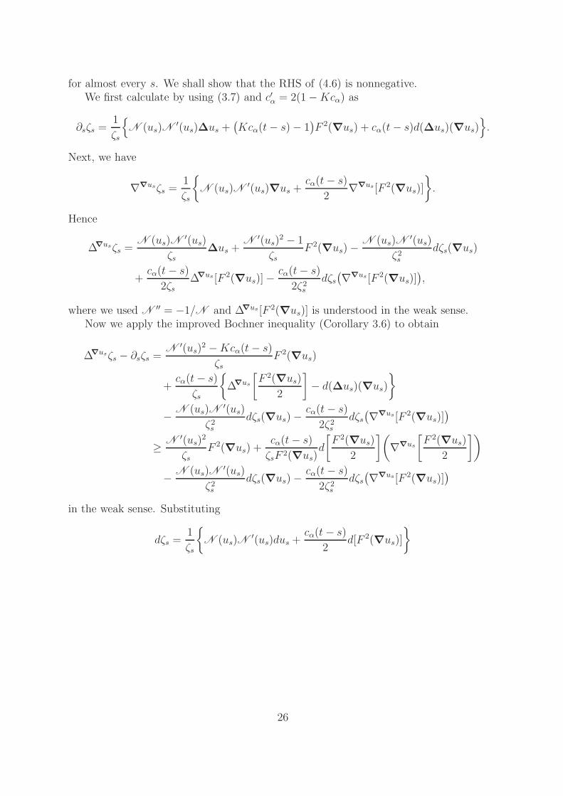
for almost every s. We shall show that the RHS of (4.6) is nonnegative.We first calculate by using (3.7) and c′α = 2(1−Kcα) as
∂sζs =1
ζs
{N (us)N
′(us)∆us +(Kcα(t− s)− 1
)F 2(∇us) + cα(t− s)d(∆us)(∇us)
}.
Next, we have
∇∇usζs =1
ζs
{N (us)N
′(us)∇us +cα(t− s)
2∇∇us[F 2(∇us)]
}.
Hence
∆∇usζs =N (us)N
′(us)
ζs∆us +
N′(us)
2 − 1
ζsF 2(∇us)−
N (us)N′(us)
ζ2sdζs(∇us)
+cα(t− s)
2ζs∆∇us [F 2(∇us)]−
cα(t− s)2ζ2s
dζs(∇∇us [F 2(∇us)]
),
where we used N ′′ = −1/N and ∆∇us [F 2(∇us)] is understood in the weak sense.Now we apply the improved Bochner inequality (Corollary 3.6) to obtain
∆∇usζs − ∂sζs =N ′(us)
2 −Kcα(t− s)ζs
F 2(∇us)
+cα(t− s)
ζs
{∆∇us
[F 2(∇us)
2
]− d(∆us)(∇us)
}
− N (us)N′(us)
ζ2sdζs(∇us)−
cα(t− s)2ζ2s
dζs(∇∇us[F 2(∇us)]
)
≥ N ′(us)2
ζsF 2(∇us) +
cα(t− s)ζsF 2(∇us)
d
[F 2(∇us)
2
](∇∇us
[F 2(∇us)
2
])
− N (us)N′(us)
ζ2sdζs(∇us)−
cα(t− s)2ζ2s
dζs(∇∇us[F 2(∇us)]
)
in the weak sense. Substituting
dζs =1
ζs
{N (us)N
′(us)dus +cα(t− s)
2d[F 2(∇us)]
}
26

and recalling (2.10), we obtain
∆∇usζs − ∂sζs ≥ζ2sN
′(us)2 −N 2(us)N
′(us)2
ζ3sF 2(∇us)
− cα(t− s)N (us)N′(us)
ζ3sdus
(∇∇us[F 2(∇us)]
)
+cα(t− s)
ζ3s
{ζ2s
F 2(∇us)− cα(t− s)
}d
[F 2(∇us)
2
](∇∇us
[F 2(∇us)
2
])
=cα(t− s)N ′(us)
2
ζ3sF 4(∇us)
− cα(t− s)N (us)N′(us)
ζ3sdus
(∇∇us[F 2(∇us)]
)
+cα(t− s)
ζ3s
N 2(us)
F 2(∇us)d
[F 2(∇us)
2
](∇∇us
[F 2(∇us)
2
]).
Since the Cauchy–Schwarz inequality for g∇usyields
∣∣dus(∇∇us[F 2(∇us)]
)∣∣ ≤ F (∇us)√d[F 2(∇us)]
(∇∇us[F 2(∇us)]
),
we conclude that
∆∇usζs − ∂sζs
≥ cα(t− s)N ′(us)2
ζ3sF 4(∇us)
− cα(t− s)N (us)|N ′(us)|ζ3s
F (∇us)√d[F 2(∇us)]
(∇∇us[F 2(∇us)]
)
+cα(t− s)
ζ3s
N 2(us)
F 2(∇us)d
[F 2(∇us)
2
](∇∇us
[F 2(∇us)
2
])
=cα(t− s)
ζ3s
(|N ′(us)|F 2(∇us)−
N (us)
2F (∇us)
√d[F 2(∇us)]
(∇∇us[F 2(∇us)]
))2
≥ 0
in the weak sense. Notice that, similarly to the proof of Theorem 3.7, we can taketest functions from H1
0 (M) ∩ L∞(M) by virtue of (3.6). Therefore the RHS of (4.6) isnonnegative and this completes the proof. ✷
When K > 0, choosing α = K−1 and letting t→∞ in (4.5) yields the following.
Corollary 4.5 Assume that (M,F,m) is complete and satisfies Ric∞ ≥ K > 0, CF <∞,
SF <∞ and m(M) = 1. Then, for any u ∈ C∞c (M) with 0 ≤ u ≤ 1 and satisfying (3.6),we have √
KN
(∫
M
u dm
)≤
∫
M
√KN 2(u) + F 2(∇u) dm. (4.7)
27

Proof. Let (ut)t≥0 be the global solution to the heat equation with u0 = u. Takingα = K−1, we find cα ≡ K−1 and hence by (4.5)
√KN 2(ut) ≤
√KN 2(ut) + F 2(∇ut) ≤ P∇u
0,t
(√KN 2(u) + F 2(∇u)
).
Letting t→∞, we deduce from the ergodicity (Proposition 4.3) that
ut →∫
M
u dm,
P∇u0,t
(√KN 2(u) + F 2(∇u)
)→
∫
M
√KN 2(u) + F 2(∇u) dm
in L2(M). Thereby we obtain (4.7). ✷
4.3 Proof of Theorem 4.1
Proof. Let θ ∈ (0, 1). Fix a closed set A ⊂M with m(A) = θ and consider
uε(x) := max{1− ε−1d(x,A), 0}, ε > 0.
Note that F (∇uε) = ε−1 on B−(A, ε)\A, where B−(A, ε) := {x ∈M | infy∈A d(x, y) < ε}is the backward ε-neighborhood of A. Applying (4.7) to (smooth approximations of) uε
and letting ε ↓ 0 implies, with the help of N (0) = N (1) = 0,
√KN (θ) ≤ lim inf
ε↓0
m(B−(A, ε))−m(A)
ε.
This is the desired isoperimetric inequality for the reverse Finsler structure←−F (recall
Definition 2.7) since, with c := ϕ−1(θ)/√K,
√KN (θ) =
√K
2πe−Kc2/2, θ = ϕ(
√Kc) =
√K
2π
∫ c
−∞
e−Ka2/2 da.
Because the curvature bound Ric∞ ≥ K is common to F and←−F , we also obtain (4.1). ✷
References
[AGS1] L. Ambrosio, N. Gigli and G. Savare, Metric measure spaces with Riemannian Riccicurvature bounded from below. Duke Math. J. 163 (2014), 1405–1490.
[AGS2] L. Ambrosio, N. Gigli and G. Savare, Bakry–Emery curvature-dimension condition andRiemannian Ricci curvature bounds. Ann. Probab. 43 (2015), 339–404.
[AM] L. Ambrosio and A. Mondino, Gaussian-type isoperimetric inequalities in RCD(K,∞)probability spaces for positive K. Atti Accad. Naz. Lincei Rend. Lincei Mat. Appl. 27(2016), 497–514.
28

[Au] L. Auslander, On curvature in Finsler geometry. Trans. Amer. Math. Soc. 79 (1955),378–388.
[Ba] D. Bakry, L’hypercontractivite et son utilisation en theorie des semigroupes. (French)Lectures on probability theory (Saint-Flour, 1992), 1–114, Lecture Notes in Math.,1581, Springer, Berlin, 1994.
[BE] D. Bakry and M. Emery, Diffusions hypercontractives. (French) Seminaire de proba-bilites, XIX, 1983/84, 177–206, Lecture Notes in Math., 1123, Springer, Berlin, 1985.
[BGL] D. Bakry, I. Gentil and M. Ledoux, Analysis and geometry of Markov diffusion opera-tors. Springer, Cham, 2014.
[BL] D. Bakry and M. Ledoux, Levy–Gromov’s isoperimetric inequality for an infinite-dimensional diffusion generator. Invent. Math. 123 (1996), 259–281.
[BCS] D. Bao, S.-S. Chern and Z. Shen, An introduction to Riemann-Finsler geometry.Springer-Verlag, New York, 2000.
[Bob1] S. Bobkov, A functional form of the isoperimetric inequality for the Gaussian measure.J. Funct. Anal. 135 (1996), 39–49.
[Bob2] S. G. Bobkov, An isoperimetric inequality on the discrete cube, and an elementary proofof the isoperimetric inequality in Gauss space. Ann. Probab. 25 (1997), 206–214.
[Bor] C. Borell, The Brunn–Minkowski inequality in Gauss space. Invent. Math. 30 (1975),207–216.
[CM] F. Cavalletti and A. Mondino, Sharp and rigid isoperimetric inequalities in metric-measure spaces with lower Ricci curvature bounds. Invent. Math. 208 (2017), 803–849.
[Ch+] B. Chow, S.-C. Chu, D. Glickenstein, C. Guenther, J. Isenberg, T. Ivey, D. Knopf,P. Lu, F. Luo, L. Ni, The Ricci flow: techniques and applications. Part I. Geometricaspects. American Mathematical Society, Providence, RI, 2007.
[CMS] D. Cordero-Erausquin, R. J. McCann and M. Schmuckenschlager, A Riemannian inter-polation inequality a la Borell, Brascamp and Lieb. Invent. Math. 146 (2001), 219–257.
[EKS] M Erbar, K. Kuwada and K.-T. Sturm, On the equivalence of the entropic curvature-dimension condition and Bochner’s inequality on metric measure spaces. Invent. Math.201 (2015), 993–1071.
[Ev] L. C. Evans, Partial differential equations. American Mathematical Society, Providence,RI, 1998.
[GS] Y. Ge and Z. Shen, Eigenvalues and eigenfunctions of metric measure manifolds. Proc.London Math. Soc. (3) 82 (2001), 725–746.
[Gi1] N. Gigli, On the differential structure of metric measure spaces and applications. Mem.Amer. Math. Soc. 236 (2015), no. 1113.
[Gi2] N. Gigli, The splitting theorem in non-smooth context. Preprint (2013). Available atarXiv:1302.5555
29

[GKO] N. Gigli, K. Kuwada and S. Ohta, Heat flow on Alexandrov spaces, Comm. Pure Appl.Math. 66 (2013), 307–331.
[Gr] M. Gromov, Metric structures for Riemannian and non-Riemannian spaces. Based onthe 1981 French original. With appendices by M. Katz, P. Pansu and S. Semmes. Trans-lated from the French by Sean Michael Bates. Birkhauser Boston, Inc., Boston, MA,1999.
[Kl] B. Klartag, Needle decompositions in Riemannian geometry. Mem. Amer. Math. Soc.249 (2017), no. 1180.
[Ku] K. Kuwada, Duality on gradient estimates and Wasserstein controls. J. Funct. Anal.258 (2010), 3758–3774.
[Lee] P. W. Y. Lee, Displacement interpolations from a Hamiltonian point of view. J. Funct.Anal. 265 (2013), 3163–3203.
[Leo] G. Leoni, A first course in Sobolev spaces. American Mathematical Society, Providence,RI, 2009.
[Le1] P. Levy, Lecons d’analyse fonctionnelle. Gauthier-Villars, Paris, 1922.
[Le2] P. Levy, Problemes concrets d’analyse fonctionnelle. Avec un complement sur les fonc-tionnelles analytiques par F. Pellegrino (French). 2d ed. Gauthier-Villars, Paris, 1951.
[Li] A. Lichnerowicz, Varietes riemanniennes a tenseur C non negatif (French). C. R. Acad.Sci. Paris Ser. A-B 271 (1970), A650–A653.
[LM] J.-L. Lions and E. Magenes, Non-homogeneous boundary value problems and applica-tions. Vol. I. Translated from the French by P. Kenneth. Springer-Verlag, New York-Heidelberg, 1972.
[LV] J. Lott and C. Villani, Ricci curvature for metric-measure spaces via optimal transport.Ann. of Math. 169 (2009), 903–991.
[Ma] V. Maz’ya, Sobolev spaces with applications to elliptic partial differential equations.Second, revised and augmented edition. Springer, Heidelberg, 2011.
[MT] R. J. McCann and P. Topping, Ricci flow, entropy and optimal transportation. Amer.J. Math. 132 (2010), 711–730.
[Mi1] E. Milman, Sharp isoperimetric inequalities and model spaces for curvature-dimension-diameter condition. J. Eur. Math. Soc. (JEMS) 17 (2015), 1041–1078.
[Mi2] E. Milman, Beyond traditional curvature-dimension I: new model spaces for isoperimet-ric and concentration inequalities in negative dimension. Trans. Amer. Math. Soc. 369(2017), 3605–3637.
[Oh1] S. Ohta, Uniform convexity and smoothness, and their applications in Finsler geometry.Math. Ann. 343 (2009), 669–699.
[Oh2] S. Ohta, Finsler interpolation inequalities. Calc. Var. Partial Differential Equations 36(2009), 211–249.
30

[Oh3] S. Ohta, Vanishing S-curvature of Randers spaces. Differential Geom. Appl. 29 (2011),174–178.
[Oh4] S. Ohta, On the curvature and heat flow on Hamiltonian systems. Anal. Geom. Metr.Spaces 2 (2014), 81–114.
[Oh5] S. Ohta, Splitting theorems for Finsler manifolds of nonnegative Ricci curvature. J.Reine Angew. Math. 700 (2015), 155–174.
[Oh6] S. Ohta, (K,N)-convexity and the curvature-dimension condition for negative N . J.Geom. Anal. 26 (2016), 2067–2096.
[Oh7] S. Ohta, Some functional inequalities on non-reversible Finsler manifolds. Proc. IndianAcad. Sci. Math. Sci. 127 (2017), 833–855.
[Oh8] S. Ohta, Needle decompositions and isoperimetric inequalities in Finsler geometry. J.Math. Soc. Japan 70 (2018), 651–693.
[OP] S. Ohta and M. Palfia, Gradient flows and a Trotter–Kato formula of semi-convexfunctions on CAT(1)-spaces. Amer. J. Math. 139 (2017), 937–965.
[OS1] S. Ohta and K.-T. Sturm, Heat flow on Finsler manifolds. Comm. Pure Appl. Math. 62(2009), 1386–1433.
[OS2] S. Ohta and K.-T. Sturm, Non-contraction of heat flow on Minkowski spaces. Arch.Ration. Mech. Anal. 204 (2012), 917–944.
[OS3] S. Ohta and K.-T. Sturm, Bochner–Weitzenbock formula and Li–Yau estimates onFinsler manifolds. Adv. Math. 252 (2014), 429–448.
[OV] F. Otto and C. Villani, Generalization of an inequality by Talagrand and links with thelogarithmic Sobolev inequality. J. Funct. Anal. 173 (2000), 361–400.
[Qi] Z. Qian, Estimates for weighted volumes and applications. Quart. J. Math. Oxford Ser.(2) 48 (1997), 235–242.
[RR] M. Renardy and R. C. Rogers, An introduction to partial differential equations. Secondedition. Springer-Verlag, New York, 2004.
[vRS] M.-K. von Renesse and K.-T. Sturm, Transport inequalities, gradient estimates, entropyand Ricci curvature. Comm. Pure Appl. Math. 58 (2005), 923–940.
[Sal] L. Saloff-Coste, Uniformly elliptic operators on Riemannian manifolds. J. DifferentialGeom. 36 (1992), 417–450.
[Sav] G. Savare, Self-improvement of the Bakry–Emery condition and Wasserstein contractionof the heat flow in RCD(K,∞) metric measure spaces. Discrete Contin. Dyn. Syst. 34(2014), 1641–1661.
[Sh] Z. Shen, Lectures on Finsler geometry. World Scientific Publishing Co., Singapore, 2001.
[St1] K.-T. Sturm, On the geometry of metric measure spaces. I. Acta Math. 196 (2006),65–131.
31

[St2] K.-T. Sturm, On the geometry of metric measure spaces. II. Acta Math. 196 (2006),133–177.
[St3] K.-T. Sturm, Super-Ricci flows for metric measure spaces. J. Funct. Anal. 275 (2018),3504–3569.
[SC] V. N. Sudakov and B. S. Cirel’son, Extremal properties of half-spaces for sphericallyinvariant measures. (Russian) Problems in the theory of probability distributions, II.Zap. Naucn. Sem. Leningrad. Otdel. Mat. Inst. Steklov. (LOMI) 41 (1974), 14–24, 165.
[Vi] C. Villani, Optimal transport, old and new. Springer-Verlag, Berlin, 2009.
[WX] G. Wang and C. Xia, A sharp lower bound for the first eigenvalue on Finsler manifolds.Ann. Inst. H. Poincare Anal. Non Lineaire 30 (2013), 983–996.
[Wy] W. Wylie, A warped product version of the Cheeger–Gromoll splitting theorem. Trans.Amer. Math. Soc. 369 (2017), 6661–6681.
[Xi] C. Xia, Local gradient estimate for harmonic functions on Finsler manifolds. Calc. Var.Partial Differential Equations 51 (2014), 849–865.
[YH] S.-T. Yin and Q. He, The first eigenvalue of Finsler p-Laplacian. Differential Geom.Appl. 35 (2014), 30–49.
32