ashland forest resiliency stewardship project: ashland...
TRANSCRIPT

1
Ashland Forest Resiliency Stewardship Project:
Ashland Creek Watershed Water Quality and Biological Assessment
June 15, 2017
Peter C. Schroeder, Ph.D.
Submitted to
the Oregon Department of Forestry’s Federal Forest Restoration Program
by The Nature Conservancy in fulfillment of agreement ODF-2191A-14 #13
Suggested citation: Schroeder, P.C. 2017. Ashland Forest Resiliency Stewardship Project: Ashland Creek Watershed Water Quality and Biological Assessment. ODF Agreement 2191A-14 #13. The Nature Conservancy, Portland, OR. 35 p.

2
Ashland Forest Resiliency Stewardship Project
Ashland Creek Watershed Water Quality and Biological Assessment
September 26, 2017
Peter C. Schroeder, Ph.D.
ABSTRACT
Between 2010 and 2015, physical and riparian habitat, hydrological factors, and aquatic macroinvertebrate samples were gathered and used to assess the biological integrity and functionality of each of four stream reaches within the Ashland Creek watershed. This analysis provides a baseline for evaluating future changes (if any) in water quality concurrent with Ashland Forest Resiliency Stewardship Project activities (forest thinning and controlled burns) in the watershed. Results from this study showed that total aquatic macroinvertebrate abundance and richness was commensurate with high biotic integrity in all streams except one (South Section 20) whose biotic condition may have been limited by a lack of substrate complexity and by a seasonally low or intermittent stream flow. The lack of significant changes in total abundance and richness of macroinvertebrates during the sampling period suggested that all sampled streams provided functionally stable habitats. However, significant changes were detected in select macroinvertebrate groups (intolerant/tolerant and functional feeding groups) in three of the four sampled streams and Hilsenhoff Biotic Index (HBI) scores significantly increased in one stream reach (East Fork Ashland Creek). These changes may signal minor or early effects of emerging biological stressors, namely shifts in the proportion of organic matter inputs from coarser to finer material (East Fork Ashland Creek) and/or gradual stream water warming (West Fork Ashland Creek and Reeder Gulch), that were possibly precipitated or exacerbated by a ensuing regional drought and associated above-normal summer (August) air temperatures recorded from 2011 thru 2015.
INTRODUCTION
The biotic condition of a stream depends upon several interacting ecological factors: stream water parameters (e.g., flow rate and chemistry), physical and riparian habitat characteristics (e.g., substrate particle types, pool depth, shading, and organic matter inputs), and biological communities (i.e., vertebrate and macroinvertebrate abundance and diversity). Physical and riparian habitat, hydrological factors, and aquatic macroinvertebrates were sampled/recorded at four stream sites (reaches) within the Ashland Creek Watershed as part of the Ashland Forest Resiliency Stewardship Project’s (AFR) adaptive management strategy (Section C-1 of the Ashland Forest Resiliency Technical Proposal Appendix TP-A). These data - collected over the six-year monitoring period from 2010 through 2015 at the time of this report - were used to provide biological assessment scores and indices for each stream reach and compare trends in various stream-related parameters across the sampling period, and summarize the analysis relative to monitored macroinvertebrate, substrate, riparian habitat, and hydrological conditions. This study sought to provide a rigorous baseline analysis of the status and trends in current stream function and condition within the Ashland Creek watershed that may include the effect of treatments on stream health within the watershed.
METHODS
Sampling Sites
Water quality monitoring samples and/or measurements (substrate particle counts, coarse woody debris, canopy closure, flow rate, residual pool depth, and aquatic macroinvertebrates) were taken along a 150-meter long reach established at the base of four different sub-watersheds within the larger Ashland Creek Watershed: East Fork Ashland Creek, West Fork Ashland Creek, Reeder Gulch, and an unnamed tributary of Ashland Creek herein called South Section 20 (Table 1; Figure 1). Streams and stream reaches were located downstream from planned AFR management activities (density management, surface and ladder fuel reduction, and controlled burning). A no-treatment riparian buffer of 300 feet was placed on all perennial streams for density management treatments and 100 feet for surface and ladder treatments. All four streams resided in forested mid-montane landscapes with elevations

3
ranging from 856 to 899 m and were classified as 1st order (Reeder Gulch and South Section 20) or 2nd order (East and West Forks of Ashland Creek) streams.
Table 1. Downstream and upstream sample reach coordinates and elevations, watershed size, and percent of AFR density management (DM) and ladder fuel treatment (SL) areas within the Ashland Creek watershed.
Stream/Watershed
Downstream Coordinates Upstream Coordinates Elev.
(m) Watershed (hectares)
Treatment Area (hectares)
Treatment Area (%) Latitude Longitude Latitude Longitude
East Fork Ashland Creek 42.1523 -122.711 42.1522 -122.710 887 12,822 1,870 15%
Reeder Gulch 42.1555 -122.723 42.1541 -122.724 883 1,166 297 25%
South Section 20 42.1589 -122.719 42.1584 -122.720 856 422 18 4% West Fork Ashland Creek 42.1489 -122.716 42.1488 -122.717 899 16,682 1,814 11%
Aquatic Macroinvertebrates
To monitor for changes in the biological integrity of the stream habitats, samples of aquatic macroinvertebrates were taken generally in the late fall or winter and annually between and including the sample “years” 2010 and 2015 (Table 2). Eight separate 1-ft2 samples were gathered from each stream reach using a 500-micron2 mesh Surber sampler placed at randomly-determined locations within targeted riffle habitats. Sampling began at the downstream end of each reach and proceeded upstream with samples spaced 10 to 15 m apart between the downstream and upstream limits of each reach. Contents of each sample were first placed in a 5-gallon bucket with clean stream water and any large debris (rocks, leaves, sticks, etc.) removed by hand before the sample was sieved using a 500-micron2 mesh screen, transferred to a 1-liter Nalgene bottle, and preserved in 90% ETOH. Individual samples from each of the four stream reaches were composited into a single 8-ft2 (0.74-m2) sample in the field. Preserved samples were then examined in a lab at SOU where all or a quantitatively representative subsample of at least 500 macroinvertebrate specimens were removed from each sample and preserved separately in glass vials containing 70% ETOH. Preserved macroinvertebrates were sent to the BLM/USU National Aquatic Monitoring Center (NAMC) for specimen identification and counts. To allow for between-site and between-year analysis and comparisons across all stream sites and sample years, taxa identifications were standardized into operational taxonomic units (OTUs) before computing data metrics on taxa abundance and richness, taxa ratios, biological assessment scores, and diversity/biotic condition indices (Hilsenhoff Biotic Index and Community Tolerance Quotient). Metrics and diversity/biotic indices used in this analysis were computed using formulas reported and cited by the BLM/USU National Aquatic Monitoring Center (https://www.usu.edu/buglab/Content/Metadata_accompanyingPDF2.pdf). See Appendix for specific scoring criteria and methods used in computing biological assessment scores.
Table 2. Stream site sample dates for each “year” of the sampling period.
Stream 2010 2011 2012 2013 2014 2015
East Fork Ashland Creek Oct 26, 2010 Nov 13, 2011 Oct 21, 2012 Dec 2, 2013 Nov 8, 2014 Feb 7, 2016
Reeder Gulch Oct 30, 2010 Nov 13, 2011 Oct 21, 2012 Dec 2, 2013 Nov 8, 2014 Feb 7, 2016
South Section 20 Nov 9, 2010 Nov 13, 2011 Oct 21, 2012 Dec 2, 2013 Nov 8, 2014 Feb 7, 2016
West Fork Ashland Creek Oct 26, 2010 Nov 13, 2011 Oct 21, 2012 Dec 2, 2013 Nov 8, 2014 Feb 7, 2016
Trends (patterned increases or declines) in macroinvertebrate counts (abundances) and metrics across the six-year sampling period were investigated using linear regression on the computed metrics of each site and year followed by a t-test of the computed slope against 0 (no slope). Although the ‘2015’ sample occurred significantly outside of the established sampling period for the fall sampling protocol used in this analysis (October thru November), macroinvertebrate taxa assemblages observed in 2015 did not significantly differ to those of previous years so the data were included in this analysis. To investigate generalized metric trends over the sampling period, the sampling

4
period was divided into first and second halves (2010 thru 2012, and 2013 thru 2015, respectively) and the mean counts or metrics for the two half-periods for each site were compared using a t-test. Because samples were not replicated within each site in each sample year (thereby making site comparisons within a given year impossible), two separate one-way analysis of variance tests were used to look for differences in metrics between sites across all years and between years across all sites. These multiple statistical tests on a single dataset may have inflated the Type I error rate in the analysis. Therefore, care was taken when interpreting significant results from these individual tests. Counts (Y) were transformed to ln(Y) to improve normal distribution of the data and correct for heteroscedasticity prior to testing. Computed test statistics (t- and F-values) were compared against the appropriate critical t- or F-value of each test and considered statistically significant when P < 0.05 and marginally significant when P < 0.10.
Physical and Riparian Habitat
Substrate Types and Particle Counts
To monitor for changes in in-stream substrate composition and complexity (and therefore potential changes in food and sheltering resources for macroinvertebrates and the tendency for substrate resorting and/or winter scouring), stream substrate types were initially categorized and recorded by particle size based on a modified Wentworth scale (Wentworth 1922) that sorted particles by the width of their narrowest axis (Table 3). Particle counts were conducted annually at each stream site between 2010 and 2015 by tallying the substrate type encountered off the toe of the wader’s boot at 100 arbitrarily-chosen sample points roughly one meter apart as the wader waded upstream in a zig-zag pattern beginning at the furthest downstream point in each stream reach (Bevenger and King 1995). To better reflect the use of substrate by aquatic macroinvertebrates, particles sizes were reclassified prior to analysis into broader substrate types (fines, gravel, cobble, boulder, bedrock, separated by fine lines in Table 3). Particle counts for substrate types were summed across years for each sample reach and compared between sample reaches using a contingency Goodness-of-Fit test. Mean particle counts were summed for broader substrate types and compared across all sample sites and years using a two-way analysis variance of variance.
Table 3. Substrate type categories and particle size ranges based on the Wentworth scale (Wentworth 1922) used in this study. Substrate particles with a less than 2 mm diameter were consolidated into a single category labeled ‘fines’ and those greater than 4096 mm in diameter were categorized as ‘bedrock’ in both the finer and broader substrate type classifications.
Substrate Type Particle size range (mm)
Fines (Sand, Silt, Clay) < 2
Very Fine Gravel 2 - 4
Fine Gravel 4 - 5.7
Fine Gravel 5.7 - 8
Medium Gravel 8 - 11.3
Medium Gravel 11.3 - 16
Coarse Gravel 16 - 22.6
Coarse Gravel 22.6 - 32
Very Coarse Gravel 32 - 45
Very Coarse Gravel 45 - 64
Small Cobble 64 - 90
Small Cobble 90 - 128
Large Cobble 128 - 180
Large Cobble 180 - 256

5
Small Boulder 256 - 362
Small Boulder 362 - 512
Medium Boulder 512 - 1024
Large Boulder 1024 - 2048
Very Large Boulder 2048 - 4096
Bedrock > 4096
Residual Pool Depths
Decreased residual pool depths are a possible indicator of increased sedimentation rates. Therefore, residual pool depths were estimated to the nearest centimeter annually between 2010 and 2015 in all distinct stream pools identified within each stream reach by calculating the difference between the maximum and the tail crest depths of each pool. Pools were expected to change with flow conditions and were not permanently marked. Mean residual pool depths were compared between stream sites, sample years, and site by sample year using a two-way variance of variance.
In-Stream Large Woody Debris
To monitor for changes in in-stream structure and complexity, large pieces of downed wood - or large woody debris (LWD) - touching the active stream channel (defined as the area of the stream bed that continuously or periodically contains water during normal stream flow) whose maximum diameter measured at least 12” and length measured at least 25 feet were tallied within the entire sample reach of each stream. Counts of LWD were converted to ln(counts) and compared between stream sites and years using a two-way analysis variance of variance.
Canopy Cover
To evaluate potential differences in canopy cover among reaches, canopy cover was calculated from 2006 LiDAR data collected by Watershed Sciences and summarized to a 5 m raster grid (available at https://tnc.box.com/s/ofzbgx5kofu38gsxgoyuu3l1bs0b86mw). The four 150 m long sample reaches were buffered by 15.2 m, consistent with riparian reserves established under the AFR Record of Decision. Percent canopy cover was estimated by averaging the raster cells that intersected the 30.4 m wide belt transects centered on the sampled reaches.
Stream Hydrology
Flow Rate
To monitor for changes in stream flow rates (and therefore the potential for substrate resorting and/or scouring during high-water events and/or the possible source of changes in summertime water temperature during to lower flows), hourly discharge rates from East Fork Ashland Creek were obtained through the USGS National Water Information System: Web Interface (https://waterdata.usgs.gov/nwis/uv/?site_no=14353500&agency_cd=USGS). Data were captured and recorded as cubic feet per second at an established USGS gauging station located at the downstream end of that stream’s sampling reach. Mean daily discharge rates were computed from the raw hourly data and plotted over the sampling period to determine seasonal patterns in flow rates and to identify incidences of high water events. Although stream flow data were not available at the other stream sites within this study, general trends (i.e., increases and declines) in stream flow rates in East Fork Ashland Creek were extrapolated to these other sites when attempting to interpret changes in stream metrics related to stream flow (i.e., temperature, scour, and resorting).
Temperature
To monitor changes in stream temperatures that may relate to changes in macroinvertebrate assemblages (namely cold-water or Class O taxa), stream water temperatures recorded by USGS personnel were examined during the study period in East and West Fork of Ashland Creek. Temperatures were recorded roughly every other month (no

6
more than 3 months between readings) using an Oakton thermistor and an acoustic meter (Flowtracker) and in most cases both reading types were taken within 4 hours of noon (earliest: 0812 h, latest: 1657 h). Oakton thermistor gave instantaneous readings while the Flowtracker meter gave mean readings over a roughly 30-minute period (shortest: 0:26, longest: 1:12). Thermistors were regularly checked by USGS for agreement with NIST standards. Readings were unpublished at the time of this report and should be considered provisional.
RESULTS
Aquatic Macroinvertebrates
Total Abundance
Total abundance of macroinvertebrates based on raw counts across all stream sites and sample years ranged from a maximum of 2643/m2 at Reeder Gulch in 2010 to a minimum of 189/m2 at South Section 20 in 2013 (Figure 2). No significant differences were detected between mean total abundance of sampled macroinvertebrates between sites (F = 0.21, df = 5, P = 0.127) or between sample years (F = 0.94 df = 5, P = 0.480). Similar results were found for total abundance of macroinvertebrates based on OTU counts: macroinvertebrate counts ranged from a maximum of 2384/m2 at Reeder Gulch in 2010 to a minimum of 170/m2 at South Section 20 in 2013; no significant differences were detected between overall mean total abundance of macroinvertebrates between sites (F = 0.21, df = 5, P = 0.136) or between sample years (F = 0.98, df = 5, P = 0.458.
Linear regression analyses of both raw or OTU counts showed no statistically significant increase or decrease (slope <> 0) in the total abundance of macroinvertebrates across all sample years for any of the four sites sampled (Table 4). When sample years were grouped into first and second halves of the sample period, no statistically significant differences in total mean abundance of macroinvertebrates were detected between the two sample periods for any of the four sites sampled (Table 5).
Table 4. Slope, t, and P-value from individual tests of linear regression of total raw and standardized OTU abundance counts of macroinvertebrates computed across all sample dates for each of the four sample sites.
Site Slope t p-value Raw Counts East Fork Ashland Creek 0.068 0.83 0.451 West Fork Ashland Creek 0.068 1.33 0.256 South Section 20 -0.144 0.96 0.389 Reeder Gulch -0.256 1.34 0.252
OTU Counts East Fork Ashland Creek 0.074 0.89 0.426 West Fork Ashland Creek 0.084 1.50 0.209 South Section 20 -0.135 0.86 0.437 Reeder Gulch -0.246 1.31 0.260
Table 5. Computed t and P values from t-tests comparing the mean total raw and standardized OTU macroinvertebrate abundance counts between first half (2010 – 2012) and second half (2013 – 2015) of the sampling period for each of the four sample sites.
Site 2010-2012 Mean ± se
2013-2015 Mean ± se t p-value
Raw Counts East Fork Ashland Creek 549 ± 126.3 790 ± 28.9 1.87 0.135 West Fork Ashland Creek 665 ± 119.2 781 ± 33.9 1.03 0.362 South Section 20 449 ± 174.0 346 ± 153.1 0.55 0.609 Reeder Gulch 1368 ± 646.3 797 ± 367.3 0.82 0.460

7
All sites 758 ± 183.2 679 ± 103.2 0.29 0.784 OTU Counts East Fork Ashland Creek 521 ± 121.9 763 ± 33.3 1.92 0.127 West Fork Ashland Creek 561 ± 106.1 711 ± 26.4 1.39 0.236 South Section 20 416 ± 169.7 328 ± 146.1 0.46 0.667 Reeder Gulch 1229 ± 581.6 736 ± 324.7 0.79 0.476 All sites 682 ± 164.9 635 ± 93.4 0.12 0.912
EPT, intolerant and tolerant taxa
Linear regression analyses for OTU counts across all sample dates revealed no statistically significant increase or decline (Slope <> 0) in the abundance of EPT taxa at any of the four sampled stream sites (Table 6; Figure 3). Intolerant and tolerant taxa, however, significantly declined in Reeder Gulch (t = -0.49, df = 4, P = 0.0066 and t = -0.96, df = 4, P = 0.0087, respectively), while no other stream site showed a statistically significant change in the abundance of these taxa when tested across all sample years. When sample years were grouped into first and second halves of the sample period, t-tests comparing the two sample periods revealed no significant change in the abundance of EPT, intolerant, or tolerant taxa. Tolerant taxa sampled from Reeder Gulch, when expressed as a percentage of the total abundance of taxa, however, showed a significant change (decline) in abundance over the sampling period (t = 2.93, df = 4, P = 0.0427).
Table 6. Slope, t, and P-values from individual tests of linear regression of standardized (OTU) abundance counts of EPT, intolerant and tolerant taxa computed across all sample dates for each of the four sample sites.
Taxa/Site Slope t p-value EPT taxa East Fork Ashland Creek 0.0833 1.03 0.360 West Fork Ashland Creek 0.1772 2.09 0.105 South Section 20 -0.1648 0.83 0.455 Reeder Gulch -0.2396 1.37 0.242 Intolerant taxa East Fork Ashland Creek -0.3367 1.94 0.124 West Fork Ashland Creek -0.1575 0.87 0.435 South Section 20 -0.3536 1.48 0.213 Reeder Gulch -0.4877 5.18 0.007
Tolerant taxa East Fork Ashland Creek 0.1415 0.46 0.670 West Fork Ashland Creek -0.1380 1.11 0.328 South Section 20 -0.1715 0.38 0.720 Reeder Gulch -0.9648 4.79 0.009
Taxa Richness
Linear regression analyses across all sample years did not reveal any statistically significant changes (slope <>0) in total, EPT, intolerant, or tolerant taxa richness counts (# of different taxa/m2) for any of the sampled stream sites (Table 7; Figure 4), although richness of intolerant taxa in South Section 20 showed a minor and marginally significant decline from 5 to 3/m2 (t = 2.62, df = 4, P = 0.059). When the sampling period was separated into first and second halves, the mean taxa richness of intolerant taxa in South Section 20 showed a minor but significant decline from 4 to 2/m2 between the two sampling periods (t = 4.10, df = 4, P = 0.015).

8
Table 7. Slope, t, and p-values from individual tests of linear regression of standardized (OTU) richness counts of EPT, intolerant and tolerant taxa computed across all sample dates for each of the four sample sites.
Taxa/Site Slope t p-value EPT taxa East Fork Ashland Creek 0.0360 0.65 0.551 West Fork Ashland Creek -0.6571 0.45 0.676 South Section 20 -0.8857 1.46 0.218 Reeder Gulch -0.7143 0.88 0.431 Intolerant taxa East Fork Ashland Creek -0.0713 0.99 0.378 West Fork Ashland Creek -1.1714 1.42 0.228 South Section 20 -0.5143 2.62 0.059 Reeder Gulch -0.0571 0.16 0.883
Tolerant taxa East Fork Ashland Creek 0.1256 0.91 0.414 West Fork Ashland Creek -0.1714 1.18 0.305 South Section 20 0.0286 0.11 0.918 Reeder Gulch -0.4000 1.25 0.280
Functional Feeding Groups
Linear regression analyses across all sample years revealed a statistically significant decline in shredders in East Fork Ashland Creek – both in counts (t = 3.25, df = 4, P = 0.0314) and as a percentage of total counts (t = 7.17, df = 4, P = 0.0020), an increase in scrapers as a percentage of total counts in East Fork Ashland Creek (t = 4.28, df = 4, P = 0.0128), an increase in scraper counts in West Fork Ashland Creek (t = 3.62, df = 4, P = 0.0224), and a decline in shredder counts in Reeder Gulch (t = 7.49, df = 4, P = 0.0017) (Table 8; Figure 5). When the sampling period was separated into first and second halves, mean counts and mean percentage of total counts of collector-gatherers and scrapers significantly increased in East Fork Ashland Creek between the two sampling periods (t = 3.20, df = 4, P = 0.0330 and t = 4.04, df = 4, P = 0.0155 for mean collector-gatherer and scraper counts, respectively, and t = 2.66, df = 4, P = 0.0565 and t = 4.28, df = 4, P = 0.0128 for collector-gatherers and scrapers as a mean percentage of total counts, respectively). No changes were detected in the richness of any functional feeding group except for a significant but minor decline from 5 to 3 taxa/m2 in collector-filterers in Reeder Gulch (t = 3.67, df = 4, P = 0.0213) (Figure 6).
Table 8. Slope, t, and P-values from individual tests of linear regression of standardized (OTU) abundance counts of predator, collector-gatherer, collector-filterer, scraper, and shredder taxa computed across all sample dates for each of the four sample sites.
Taxa/Site Slope t p-value Predator East Fork Ashland Creek -0.1443 1.50 0.209 West Fork Ashland Creek 0.1677 1.30 0.262 South Section 20 -0.2409 1.23 0.286 Reeder Gulch -0.2010 1.39 0.235 Collector-Gatherer East Fork Ashland Creek 0.1520 1.62 0.180 West Fork Ashland Creek -0.0135 0.19 0.860 South Section 20 -0.0966 0.85 0.443 Reeder Gulch -0.0745 0.26 0.808

9
Collector-Filterer East Fork Ashland Creek 0.2688 2.46 0.070 West Fork Ashland Creek 0.0769 0.69 0.529 South Section 20 0.0146 0.03 0.976 Reeder Gulch -0.2972 1.31 0.259 Scraper East Fork Ashland Creek 0.2048 1.97 0.120 West Fork Ashland Creek 0.1544 3.62 0.022 South Section 20 -0.2747 1.32 0.257 Reeder Gulch -0.1696 0.56 0.605 Shredder East Fork Ashland Creek -0.4011 3.25 0.031 West Fork Ashland Creek -0.2134 0.80 0.469 South Section 20 -0.3026 1.25 0.280 Reeder Gulch -0.5335 7.49 0.002
Taxa Ratios
Ratios of selected taxa groups were variable across the six-year sampling period (Figures 7 & 8) and only the ratio of shredders to total taxa in East Fork Ashland Creek showed a statistically significant change (decline from 0.42 to 0.03) when changes in ratios were tested (slope <>0) using linear regression (t = 3.87, df = 4, P = 0.0180) (Table 9; Figure 8). Although the ratio of EPT taxa to total taxa in East Fork Ashland Creek showed a marginally significant increase from 0.71 to 1.54 across the six-year sampling period (t = 2.69, df = 4, P = 0.0548), mean ratios of EPT taxa to total taxa computed for the same stream site showed a statistically significant increase from 0.67 to 1.47 between the first and second halves of the six-year sampling period (t = 5.76, df = 4, P = 0.0045).
Table 9. Slope, t, and P-values from individual tests of linear regression of selected taxa ratios of EPT/total, EPT/chironomids (EPT/Chir), shredders/collector-filterers (SH/CF), scrapers/(scrapers + collector-filterers) (SC/(SC+CF), and shredders/total (SH/Total) computed across all sample dates for each of the four sample sites.
Taxa/Site Slope t p-value EPT/Total East Fork Ashland Creek 0.1771 2.69 0.055 West Fork Ashland Creek 0.0549 1.77 0.151 South Section 20 0.0266 0.24 0.824 Reeder Gulch 0.0155 0.12 0.909 EPT/Chir East Fork Ashland Creek -13.9042 1.28 0.269 West Fork Ashland Creek 3.2772 0.43 0.687 South Section 20 -1.6169 1.16 0.310 Reeder Gulch -11.1076 0.65 0.550 SH/CF East Fork Ashland Creek -0.2298 0.36 0.738 West Fork Ashland Creek 0.8002 0.99 0.378 South Section 20 -0.0470 0.10 0.927 Reeder Gulch 0.2205 0.85 0.444

10
SC/(SC+CF) East Fork Ashland Creek -0.0049 0.32 0.762 West Fork Ashland Creek 0.0092 0.50 0.644 South Section 20 -0.0554 0.91 0.415 Reeder Gulch 0.0202 0.64 0.558 SH/Total East Fork Ashland Creek -0.0606 3.87 0.018 West Fork Ashland Creek -0.0154 0.84 0.446 South Section 20 -0.0065 0.22 0.836 Reeder Gulch -0.0229 0.72 0.512
Cold-water and Long-lived taxa
Cold-water adapted macroinvertebrates were present in all streams and years except West Fork Ashland Creek in 2014 and Reeder Gulch in 2014 and 2015 (Table 10). The decline of cold-water taxa observed in 2014 and 2015 contributed to a general reduction in the observed mean counts of cold-water taxa from 2 to 1 taxa observed per year during the sampling period (Figure 9).
Table 10. Cold-water adapted taxa observed in East Fork Ashland Creek (EF), West Fork Ashland Creek (WF), South Section 20 (S20), and Reeder Gulch (RG).
Cold-water taxa Stream reach (year observed)
Plecoptera
Pteronarcys princeps EF (2015)
Sierraperla cora WF (2010, 11,13)
Philocasca sp. S20 (2010)
Frisonia picticeps WF (2012)
Trichoptera
Cryptochia sp. EF (2010), WF (2013), S20 (2010)
Tinodes sp. EF (2010), RG (2010, 11, 13)
Himalopsyche phryganea EF (2010, 11, 12, 12), WF (2012)
Pedomoecus sierra WF (2011, 13, 15)
Rhyacophila grandis S20 (2011, 15), RG (2010, 12)
Rhyacophila Vofixa Gr S20 (2011, 12, 13, 14)
Rhyacophila Rotunda Gr RG (2013)
Goeracea sp. RG (2011)
Coleoptera
Bryelmis siskiyou EF (2012), WF (2012)
Diptera
Bibiocephala sp. WF (2011)

11
Long-lived taxa (taxa with 2- or more year life cycles) were found in all stream reaches and in all sample years (Table 11). Richness of long-lived taxa ranged from 3 to 7 taxa/stream/year and no significant general changes (increases or decreases) in long-lived taxa richness were detected across sample years in any stream reach.
Table 11. Long-lived taxa observed in East Fork Ashland Creek (EF), West Fork Ashland Creek (WF), South Section 20 (S20), and Reeder Gulch (RG).
Long-lived taxa Stream reach (year observed)
Odonata
Octogomphus sp. S20 (2014, 15)
Plecoptera Calineuria sp. EF (2010, 13, 14), WF (2011, 13, 14, 15), S20 (2014), RG (2012, 13, 15)
Doroneuria sp. EF (2010, 11, 12, 13, 14, 15), WF (2010, 11, 12, 13, 14, 15)
Pteronarcys sp. EF (2015), S20 (2010, 11), RG (2015)
Yoraperla sp. EF (2010, 11, 13, 14, 15), WF (2011, 12, 13, 14), S20 (2011, 12), RG (2010, 11, 12, 13, 14, 15)
Megaloptera Corydalidae (Orohermes sp.) EF (2010, 11, 13), WF (2010, 11, 12, 13, 14, 15)
Trichoptera Arctopsyche sp. EF (2010, 11, 12, 13, 14, 15), WF (2010, 12, 13, 15), RG (2012)
Parapsyche sp. EF (2012), WF (2011), S20 (2010, 11, 12, 13, 14, 15), RG (2010, 11, 12, 13)
Heteroplectron sp. WF (2013), RG (2010, 13, 14)
Coleoptera
Lara sp. EF (2011, 12, 13, 14, 15), WF (2010, 11, 12, 13, 14, 15), S20 (2010, 11, 12, 13, 14, 15), RG (2011, 12, 13)
Psephenidae (Eubrianax sp.) EF (2015), RG (2010, 12, 13,14, 15)
Biotic Indices
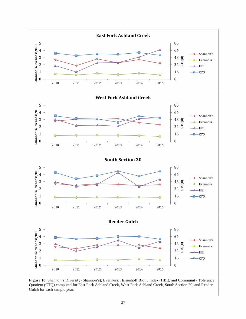
Hilsenhoff Biotic Indices (HBI) computed for each site and year were less than 3.5, the maximum level where no apparent organic pollution is indicated and water quality is considered excellent (Hilsenhoff 1987), except for two incidences where this threshold was exceeded: East Fork Ashland Creek in 2015 (4.08) and South Section 20 in 2013 (4.29). Except in East Fork Ashland Creek where the HBI increased from 1.87 to 4.08 (t = 3.68, df = 4, P = 0.0212), no statistically significant changes in the Community Tolerance Quotient, Shannon’s Diversity, Evenness, and Hilsenhoff Biotic Index (HBI) were detected across the six-year sampling period for the sampled stream sites (Table 12; Figure 10). Also, no significant differences in any of the measured biological indices were detected between the first and second half of the sampling period.
Table 12. Slope, t, and P-values for individual tests of linear regression of Community Tolerance Quotient (CTQ), Shannon’s Diversity, Evenness, and Hilsenhoff Biotic Index (HBI) computed across all sample dates for each of the four sample sites.
Taxa/Site Slope t p-value CTQ East Fork Ashland Creek -0.0814 0.11 0.915 West Fork Ashland Creek -0.5714 0.42 0.698 South Section 20 1.2159 0.69 0.527 Reeder Gulch 0.0696 0.10 0.928

12
Shannon’s Diversity East Fork Ashland Creek -0.0115 0.11 0.914 West Fork Ashland Creek -0.1084 1.57 0.191 South Section 20 -0.0204 0.82 0.460 Reeder Gulch 0.0138 0.22 0.836 Evenness East Fork Ashland Creek -0.0034 0.13 0.906 West Fork Ashland Creek -0.0197 1.34 0.251 South Section 20 0.0003 0.05 0.960 Reeder Gulch 0.0177 1.12 0.324 HBI East Fork Ashland Creek 0.4926 3.68 0.021 West Fork Ashland Creek 0.1148 0.86 0.437 South Section 20 0.0974 0.50 0.643 Reeder Gulch 0.1199 0.85 0.442
Biotic Assessment Scores
Although linear regression analyses across all sample years did not reveal any statistically significant changes (slope <>0) in biological assessment scores for any of the sampled stream sites (Table 13; Figure 11), comparisons between the first and second halves of the six-year sampling period showed that mean negative scores computed for East Fork Ashland Creek significantly declined from 92.52 to 85.71 (t = 3.16, df = 4, P = 0.0341), mean negative scores computed for West Fork Ashland Creek significantly increased from 86.39 to 91.84 (t = 4.00, df = 4, P = 0.0161), overall scores computed for South Section 20 significantly declined from 61.56 to 49.19 (t = 3.31, df = 4, P = 0.0296), and positive scores computed for South Section 20 significantly declined from 45.03 to 25.73 (t = 5.35, df = 4, P = 0.0059).
Table 13. Slope, t, and P-values for individual tests of linear regression of overall, primary, positive, and negative scores computed across all sample dates for each of the four sample sites.
Taxa/Site Slope t p-value Primary Score East Fork Ashland Creek -0.7937 0.23 0.828 West Fork Ashland Creek -3.8095 0.59 0.584 South Section 20 -1.7460 0.94 0.399 Reeder Gulch -3.6508 2.39 0.075 Positive Score East Fork Ashland Creek -2.9574 1.49 0.209 West Fork Ashland Creek -6.2155 1.94 0.124 South Section 20 -4.2607 2.00 0.117 Reeder Gulch -1.7043 0.87 0.432 Negative Score East Fork Ashland Creek -1.7493 2.22 0.091 West Fork Ashland Creek 1.2828 2.08 0.106 South Section 20 -1.8659 1.25 0.279 Reeder Gulch 0.8163 0.61 0.577

13
Overall Score East Fork Ashland Creek -2.1659 1.77 0.151 West Fork Ashland Creek -2.9032 1.16 0.310 South Section 20 -2.9493 1.95 0.124 Reeder Gulch -0.9908 1.10 0.332
Physical and Riparian Habitat
Substrate Types and Particle Counts
Particle counts varied significantly between the broader-defined substrate types (fines, gravel, cobble, boulder, and bedrock) when these counts were averaged across all sample sites and years (Table 14). Gravel (2 – 64 mm) dominated the mean particle counts at all the sample sites (Figure 12). However, median substrate types ranged from fine gravel (4 – 5.7 mm) to bedrock (> 4096 mm) across all sites and years (Table 15). East Fork Ashland Creek was the only stream site that contained an overall median substrate type that wasn’t gravel (small 64 – 90 mm cobble), while the overall median substrate type at all the other sites ranged from fine (4 – 5.7 mm) to very coarse gravel (45 – 60 mm). Summed particle counts significantly differed between samples sites for all broader-defined substrate types (Table 16). When compared with all other sites, South Section 20 possessed the greatest particle counts of fines and gravel as well as the least particle counts of cobble, East Fork Ashland Creek and Reeder Gulch possessed the greatest particle counts of bedrock, and West Fork Ashland Creek possessed the greatest particle counts of boulder, while Reeder Gulch possessed the least particle counts of boulder.
Table 14. Analysis of variance table for the effect of broader substrate type on mean substrate particle counts across all sites and years.
Source SS d.f. MS F p-value Substrate Type 3,507.1611 4 876.7903 8.06 0.00112 Sampling Error 1,303.1875 15 108.7361 Total 4,810.3486 19 253.1762
Table 15. Low, high, and overall median substrate types recorded in East Fork Ashland Creek, West Fork Ashland Creek, South Section 20, and Reeder Gulch. Low median = the smallest diameter median substrate type recorded across all sample years; High median = the greatest diameter median substrate type recorded across all sample years; Overall median = the median substrate type recorded across all sample years.
Site Low Median High Median Overall Median East Fork Ashland Creek Very Coarse Gravel
(45 – 60 mm) Bedrock (>4096 mm)
Small Cobble (64 – 90 mm)
West Fork Ashland Creek Coarse Gravel (22.6 – 32 mm)
Small Boulders (256 – 362 mm)
Very Coarse Gravel (45 – 60 mm)
South Section 20 Fine Gravel (4 – 5.7 mm)
Fine Gravel (5.7 – 8 mm)
Fine Gravel (4 – 5.7 mm)
Reeder Gulch Fine Gravel (4 – 5.7 mm)
Small Cobble (64 – 90 mm)
Coarse Gravel (22.6 – 32 mm)
Table 16. Goodness-of-Fit test for differences in observed vs. expected particle counts of each broader substrate type between sample sites summed for all sample years. Expected particle counts were given as those for even particle counts across all substrate types, sample streams, and sample years.
Substrate Type X2 statistic d.f. p-value
Fines 36.86 3 <0.0001
Gravel 66.32 3 <0.0001

14
Cobble 57.91 3 <0.0001
Boulder >1*10307 3 <0.0001
Bedrock >1*10307 3 <0.0001
Residual Pool Depth
Residual pool depths differed significantly between stream reaches (F = 75.58; df = 3, 100; p < 0.0001) and between sample years (F = 3.27; df = 5, 100; p < 0.0089), but no interaction between stream reach and sample year was detected (Table 17). Overall mean residual pool depths were greatest in East and West Forks of Ashland Creek (0.40 and 0.38 m, respectively) and least in South Section 20 (0.07 m) (Figure 13). Linear regression of residual pool depths against sample years suggested that residual pool depths in West Fork Ashland Creek significantly declined from 0.48 to 0.28 m between 2010 and 2015 (t = 6.90; df = 4; p = 0.0023), and that residual pool depths significantly increased in Reeder Gulch from 0.10 to 0.19 m between the same period (t = 2.80; df = 4; p = 0.0489).
Table 17. Analysis of variance table for the effect of site, sample year, and the interaction of site and sample year on mean residual pool depth.
Source SS d.f. MS F p-value
Stream Reach 6.6094 3 2.2031 75.58 <0.0001
Sample Year 0.4763 5 0.0953 3.27 0.0089
Reach x Year 0.1919 15 0.0128 0.44 0.9634
Sampling Error 2.9148 100 0.0292
Total 10.1924 123 0.0829
In-Stream Large Woody Debris
Mean number of large woody debris significantly differed between sample reaches and years (Table 18). Overall mean counts of LWD ranged between 3.6 to 9.7 pieces and were greatest in South Section 20 where it steadily increased during the sampling period (Figure 14). Other stream reaches showed no changes in LWD over the sampling period.
Table 18. Analysis of variance table for the effect of stream reach and sample year on the count of in-stream large woody debris.
Source SS
d.f. MS F p-value
Stream Reach 3.6726 3 1.2242 14.92 0.0001
Sample Year 1.4753 5 0.2951 3.60 0.0245
Sampling Error 1.2305 15 0.0820
Total 6.3785 23 0.2773
Canopy Cover
Based on LiDAR data, canopy cover was at least 75% in all stream reaches and ranged from 75.8% in Reeder Gulch to 84.7% in West Fork Ashland Creek (Table 20).
Table 20. Percent canopy cover among East Fork Ashland Creek, West Fork Ashland Creek, South Section 20, and Reeder Gulch. The sample size (N) is the number of 5 m pixels included in the analysis.

15
Stream Reach Sample size (N) Canopy cover (%) Standard Deviation
West Fork Ashland Creek 214 84.7 84.7
East Fork Ashland Creek 212 80.5 80.5
Reeder Gulch 247 75.8 75.8
South Section 20 222 79.5 79.5
Stream Hydrology
Flow Rate
East Fork Ashland Creek exhibited typical patterns in flow rate that peaked during the winter and spring periods (Figure 15), generally reflecting seasonal winter/spring rains and spring snowmelt, respectively, with mean monthly discharge rates greatest in June and least in September. Hourly discharge rates in East Fork Ashland Creek averaged 8.83 cfs overall and ranged between 1.29 and 207 cfs during the six-year sampling period. Two major high-water (>100 cfs) events occurred on December 2, 2012 and Feb 7, 2015 with peak hourly discharge rates of 207 and 164 cfs, respectively, and numerous short-lived minor “flushes” with hourly discharge rates <100 cfs predominately occurring between and including the months of December and May. Discharge rates were greatest in 2011 and least in 2014 (Figure 16).
Temperature
Stream water temperatures in East and West Forks of Ashland Creek showed typical seasonal fluctuations between winter and summer months with peak low temperatures between 0 and 4 degrees Celsius (generally during December and February) and peak high temperatures between 10 and 18 degrees Celsius (generally during July and September) (Figure 17). Although exact peak temperatures could not be identified (because of irregular and sometimes infrequent readings), the recorded maximum high temperatures during the later 3 years of the study period (2013 thru 2015) exceeded those recorded in the first 3 years of the study period (2010 thru 2012) in both stream reaches suggesting a general increase in summertime stream water temperatures in both streams during the study period. These water temperatures coincided with a concomitant increase in recorded regional summer air temperatures (Figure 18).
DISCUSSION
Because benthic stream aquatic macroinvertebrates are adapted to stream water parameters as well as the physical and riparian characteristics of a stream, the abundance as well as the taxonomic and functional diversity of macroinvertebrates found in a stream reflects (and thereby can serve as indicators to) the biological integrity of that stream (that is, the stream’s natural ability to act as a stable resource to a watershed’s health). The lack of significant differences in mean total abundance or richness of macroinvertebrates between stream sites across all sample years or between sample years across all stream sites suggested that the streams sampled in this study provided a functionally stable habitat for aquatic macroinverterbates and that periodic stressors (such as substrate resorting, scouring, or abrupt sedimentation) were absent, or were too minor to have had a significant or lasting impact on stream biotic integrity, during the sampling period. Although significant changes in both tolerant and intolerant taxa were detected in Reeder Gulch, no significant changes in EPT taxa were found during the six-year sampling period, suggesting again that biotic stressors were absent or too minor during the sampling period to have impacted the overall biotic integrity of the sampled streams. Significant fluctuations in the abundance as well as ratios of select functional feeding groups were found in East Fork Ashland Creek, West Fork Ashland Creek, and Reeder Gulch, however, these changes were within the range of normal fluctuations in streams with high or stable biotic integrity.
Biotic indices suggested no significant changes in organic enrichment, or the diversity or evenness of taxa, in the streams during the sampling period, except in East Fork Ashland Creek where the Hilsenhoff Biotic Index showed a significantly steady increase from 1.87 to 4.08. However, HBI scores less than 3.5 experientially indicate “no organic enrichment” (Hilsenhoff 1987), therefore these results suggested that organic enrichment has remained at levels still supportive of high biotic integrity. Biological assessment scores suggested no significant overall changes

16
in biotic integrity within the sampled streams. However, significant declines in negative scores in East Fork Ashland Creek between the first and second half of the sampling period reflected a steady decline in the stonefly shredder species Yoraperla with a concomitant increase in the mayfly collector-gatherer species Baetis. This shift in functional feeding groups possibly signals a shift in organic matter inputs from coarser to finer particle sizes. This assessment aligns with the witnessed increases in HBI scores (organic enrichment) for this stream. Interestingly, West Fork Ashland Creek showed an opposite, although weaker, significant trend in negative scores that reflected an overall decrease in the dominance of collector species in this stream. This trend, however, did not correlate with changes in HBI scores.
A decline in the overall biological assessment score in South Section 20 correlated with a marginal decline in the richness of intolerant species, and thus a lower assigned positive score, in this stream. This stream had the least abundance and richness of macroinvertebrates compared with the other streams in this study and was dominated by collector-gather species, most notably chironomids (Orthocladiinae). This weaker assemblage of macroinvertebrates most likely reflects the greater dominance of gravels and fines, and subsequent substrate embeddedness (and restriction of inhabitable hyporheic zones), exhibited by this stream. Also, although it contained flowing water during the sampling times of this study, South Section 20 may have become intermittent mid-summer during extremely dry years, thereby limiting the abundance of macroinvertebrates in this stream reach.
Although all sampled stream reaches were dominated by gravel, mean particle counts varied significantly between the broader-defined substrate types, with South Section 20 containing the greatest mean counts of fines and gravel, as well as the least counts of cobble and boulder compared with the other sampled stream reaches. West Fork Ashland Creek contained the greatest mean counts of boulder. The significantly lower abundance and richness of scrapers (as well as the relative percentage of this group compared to other functional feeding groups) observed in South Section 20 compared to other stream reaches reflects the relative abundance of fines and gravel and scarcity of cobble, boulder, and bedrock substrate in this stream.
The observed differences in the residual pool depths between the sample streams were expected given the differences in the sizes (orders) of the streams. East and West Fork of Ashland Creek (both 2nd order streams) contained significantly greater pool depths compared to South Section 20 and Reeder Gulch (1st order streams). Despite being a 1st order stream, Reeder Gulch exhibited an abundance and richness of aquatic macroinvertebrates comparable to the 2nd order streams East and West Fork Ashland Creek. Similarity in macroinvertebrate assemblages may be in part explained by the similarity in substrate types in the three stream reaches. However, differences in the richness of aquatic macroinvertebrate assemblages between the 1st and 2nd order streams may have been more pronounced if depositional habitats had been sampled.
All streams had some amount (3 to 12 pieces) of in-channel LWD that likely boosted biotic integrity of the streams by introducing organic matter and diversifying stream channel structure and dynamics. The measure of the influence of LWD on macroinvertebrate abundance and/or diversity may have been, however, limited by the sampling methods used in this study: aquatic macroinvertebrate sampling methods targeted riffle and not depositional habitats where such an influence may have been most pronounced. A comparison between streams that significantly differed in LWD abundance (e.g., the comparison of West Fork Ashland Creek with South Section 20 where a significantly larger number of LWD pieces were found) did not correlate with differences in the abundance or richness of functional feeding groups most dependent upon organic matter inputs – shredders and collector-gatherers. Since all stream reaches contained LWD, the affect of LWD on the biotic integrity of the sampled streams was probably similar (and therefore any differences were undetectable) across the sampled stream reaches.
Canopy cover provides shade and can limit consequent radiant warming of streams. All of the stream reaches have ample (>75%) canopy cover and the observed presence of cold-water adapted species in the sampled streams suggested that the stream reaches have adequate conditions to maintain low temperatures supportive a high biotic integrity. However, cold-water adapted species were absent in two sites (West Fork of Ashland Creek and Reeder Gulch) during the last two years of this study and a mild overall decline of the mean number of cold-water adapted species was observed in three out of the four stream sites during the sampling period. Data suggested that maximum summertime water temperatures increased during the study period, a trend that correlated with increasing regional summer air temperatures. The gradual decline in mean annual stream discharge rates between 2011 and 2014 combined with observed increases in summertime water temperatures may have contributed to the subsequent decline in cold-water adapted species residing in the streams.

17
Despite two major high-water events (detected by flow rates exceeding 100 cfs in December of 2012 and February of 2015 in East Fork Ashland Creek), scraper macroinvertebrate assemblages remained relatively stable, indicating that scouring (and the subsequent removal of substrate periphyton by suspended and mobilized sand) was not a significant biological stress factor during the sampling period.
ACKNOWLEDGMENTS
The Ashland Forest Resiliency (AFR) Stewardship Project was established in 2010 as a collaborative multi-party effort involving representatives of the City of Ashland, U.S. Forest Service (USFS), Southern Oregon University (SOU), and The Nature Conservancy (TNC) whose on-going collective task is to develop and implement forest management practices aimed to reduce the likelihood of catastrophic wildfire within the Ashland Creek Watershed as well as to monitor and protect the biological integrity of the streams within the watershed. Numerous individuals from each of these agencies have contributed meaningfully to this project and deserve ample recognition for their contributions and efforts. Among these contributors, the following deserve special recognition: Kerry Metlen, TNC Forest Ecologist, who arranged assess to the watershed each year and helped manage personnel as needed; Ian Reid, Steven Brazier, and Aaron Donnell, USFS Fisheries Biologists who each served as a contact and liason with NAMC to ensure timely macroinvertebrate identification and reporting; Eric Dinger, Aquatic Ecologist for the National Park Service Klamath Inventory and Monitoring Network, who assisted with setting initial macroinvertebrate sampling protocols and collection; Chris Chambers, City of Ashland Forest Resource Specialist, who helped coordinate and avoid conflicts between macroinvertebrate and AFR field activities; Derek Olson and Keith Perchemlides, TNC Southwest Oregon Field Ecologists, who each directed, assisted, and supervised the collection of water quality samples and data; and individual SOU Biology, Environmental Studies, and Environmental Education students (including Levi Drake, Morgyn Ellis, Kindra Hixon, Linnea Lopez, Ryan McKim, Bailee Reimer, Alena Slaughter, Sullivan Stevens, Lawrence VanEgdom, Julianna Williams) as well as the SOU students of the Fall 2011 and 2013 BI466/566 (Entomology) classes who assisted with macroinvertebrate collection and sorting.
REFERENCES CITED
Bevenger, King, 1995. A pebble count procedure for assessing cumulative watershed effects. Rocky Mountain Forest and Range Experiment Station. RM-RP-319.
Hayslip, G.A., L.G. Herger, and P. T. Leinenbach. 2004. Ecological condition of western cascades ecoregion streams. EPA 910-R-04-005. U.S. Environmental Protection Agency, Region 10, Seattle, Washington.
Hilsenhoff, W.L. 1987. An improved biotic index of organic stream pollution. Great Lakes Entomologist 20:31-39.
Lemmon, P. E. 1956. A spherical densiometer for estimating forest overstory density. Forest Science. 2: 314-320.
Strickler, G.S. 1958. Use of the densiometer to estimate density of forest canopy on permanent sample plots. USDA Forest Service Pacific Northwest Forest and Range Experiment Station, Research Note 180.
Wentworth, C. K. 1922. A scale of grade and class terms for clastic sediments. The Journal of Geology. 30 (5): 377–392.

18
FIGURES
Figure 1. AFR water quality monitoring sites, watersheds, and AFR treatment areas.

19
Figure 2. Abundance (number per m2) of aquatic macroinvertebrates based on total raw and standardized OTU counts in East Fork Ashland Creek, West Fork Ashland Creek, South Section 20, and Reeder Gulch for each sample year.
0
500
1000
1500
2000
2500
3000
2010 2011 2012 2013 2014 2015
Abun
danc
e (#
/m2 )
Total Abundance - Raw Counts
East Fork Ashland Creek West Fork Ashland Creek South Section 20 Reeder Gulch
0
500
1000
1500
2000
2500
3000
2010 2011 2012 2013 2014 2015
Abun
danc
e (#
/m2 )
Total Abundance - OTU Counts
East Fork Ashland Creek West Fork Ashland Creek South Section 20 Reeder Gulch

20
Figure 3. Abundance (number of OTU counts per m2) of EPT, intolerant, and tolerant aquatic macroinvertebrates in East Fork Ashland Creek, West Fork Ashland Creek, South Section 20, and Reeder Gulch for each sample year.
0
200
400
600
800
2010 2011 2012 2013 2014 2015
Abun
danc
e (#
/m2 )
East Fork Ashland Creek
EPT
Intolerant
Tolerant
0
200
400
600
800
2010 2011 2012 2013 2014 2015
Abun
danc
e (#
/m2 )
West Fork Ashland Creek
EPT
Intolerant
Tolerant
0
200
400
600
800
2010 2011 2012 2013 2014 2015
Abun
danc
e (#
/m2 )
South Section 20
EPT
Intolerant
Tolerant
0
400
800
1200
1600
2010 2011 2012 2013 2014 2015
Abun
danc
e (#
/m2 )
Reeder Gulch
EPT
Intolerant
Tolerant

21
Figure 4. Richness (number of OTU taxa/m2) of total, EPT, intolerant, and tolerant taxa in East Fork Ashland Creek, West Fork Ashland Creek, South Section 20, and Reeder Gulch for each sample year.
0
10
20
30
40
50
60
2010 2011 2012 2013 2014 2015
Rich
ness
(#ta
xa/m
2 )East Fork Ashland Creek
Total
EPT
Intolerant
Tolerant
0
10
20
30
40
50
60
2010 2011 2012 2013 2014 2015
Rich
ness
(#t
axa/
m2 )
West Fork Ashland Creek
Total
EPT
Intolerant
Tolerant
0
10
20
30
40
50
60
2010 2011 2012 2013 2014 2015
Rich
ness
(#t
axa/
m2 )
South Section 20
Total
EPT
Intolerant
Tolerant
0
10
20
30
40
50
60
2010 2011 2012 2013 2014 2015
Rich
ness
(#t
axa/
m2 )
Reeder Gulch
Total
EPT
Intolerant
Tolerant

22
Figure 5. Abundance (number of OTU counts/m2) of predator, collector-gatherer, collector-filterer, scraper, and shredder taxa in East Fork Ashland Creek, West Fork Ashland Creek, South Section 20, and Reeder Gulch for each sample year.
0100200300400500600700800
2010 2011 2012 2013 2014 2015
Abun
danc
e (#
/m2 )
East Fork Ashland Creek
Predator
Collector-gather
Collector-filterer
Scraper
Shredder
0100200300400500600700800
2010 2011 2012 2013 2014 2015
Abun
danc
e(#
/m2 )
West Fork Ashland Creek
Predator
Collector-gather
Collector-filterer
Scraper
Shredder
0100200300400500600700800
2010 2011 2012 2013 2014 2015
Abun
danc
e(#
/m2 )
South Section 20
Predator
Collector-gather
Collector-filterer
Scraper
Shredder
0100200300400500600700800
2010 2011 2012 2013 2014 2015
Abun
danc
e(#
/m2 )
Reeder Gulch
Predator
Collector-gather
Collector-filterer
Scraper
Shredder

23
Figure 6. Richness (number of OTU taxa) of predators, collector-gatherers, collector-filterers, scrapers, and shredders in East Fork Ashland Creek, West Fork Ashland Creek, South Section 20, and Reeder Gulch for each sample year.
0
5
10
15
20
2010 2011 2012 2013 2014 2015
Rich
ness
(#ta
xa)
East Fork Ashland Creek
Predator
Collector-gather
Collector-filterer
Scraper
Shredder
0
5
10
15
20
2010 2011 2012 2013 2014 2015
Rich
ness
(#ta
xa)
West Fork Ashland Creek
Predator
Collector-gather
Collector-filterer
Scraper
Shredder
0
5
10
15
20
2010 2011 2012 2013 2014 2015
Rich
ness
(#ta
xa)
South Section 20
Predator
Collector-gather
Collector-filterer
Scraper
Shredder
0
5
10
15
20
2010 2011 2012 2013 2014 2015
Rich
ness
(#ta
xa)
Reeder Gulch
Predator
Collector-gather
Collector-filterer
Scraper
Shredder

24
Figure 7. Ratios of EPT/chironomids (EPT/Chir) and EPT/Total taxa in East Fork Ashland Creek, West Fork Ashland Creek, South Section 20, and Reeder Gulch for each sample year.
0.0
0.5
1.0
1.5
2.0
0
50
100
150
200
2010 2011 2012 2013 2014 2015
EPT/
Tota
l
EPT/
Chir
East Fork Ashland Creek
EPT/Chir EPT/Total
0.0
0.5
1.0
1.5
2.0
0
50
100
150
200
2010 2011 2012 2013 2014 2015
EPT/
Tota
l
EPT/
Chir
West Fork Ashland Creek
EPT/Chir EPT/Total
0.0
0.5
1.0
1.5
2.0
0
50
100
150
200
2010 2011 2012 2013 2014 2015EP
T/To
tal
EPT/
Chir
South Section 20
EPT/Chir EPT/Total
0.0
0.5
1.0
1.5
2.0
0
50
100
150
200
2010 2011 2012 2013 2014 2015
EPT/
Tota
l
EPT/
Chir
Reeder Gulch
EPT/Chir EPT/Total

25
Figure 8. Ratios of scrapers/(scrapers + collector-filterers) (SC/(SC+CF)), shredders//Total (SH/Total), and shredders/collector-filterers (SH/CF) in East Fork Ashland Creek, West Fork Ashland Creek, South Section 20, and Reeder Gulch for each sample year.
0
3
6
9
12
15
0.0
0.2
0.4
0.6
0.8
1.0
2010 2011 2012 2013 2014 2015
SH/C
F
SC/(
SC+C
F) o
r SH
/Tot
alEast Fork Ashland Creek
SC/(SC+CF)
SH/Total
SH/CF
0
3
6
9
12
15
0.0
0.2
0.4
0.6
0.8
1.0
2010 2011 2012 2013 2014 2015
SH/C
F
SC/(
SC+C
F) o
r SH
/Tot
al
West Fork Ashland Creek
SC/(SC+CF)
SH/Total
SH/CF
0
3
6
9
12
15
0.0
0.2
0.4
0.6
0.8
1.0
2010 2011 2012 2013 2014 2015
SH/C
F
SC/(
SC+C
F) o
r SH
/Tot
al
South Section 20
SC/(SC+CF)
SH/Total
SH/CF
0
3
6
9
12
15
0.0
0.2
0.4
0.6
0.8
1.0
2010 2011 2012 2013 2014 2015
SH/C
F
SC/(
SC+C
F) o
r SH
/Tot
al
Reeder Gulch
SC/(SC+CF)
SH/Total
SH/CF

26
Figure 9. Number of cold-water adapted taxa by stream reach and year. Overlapping line depicts the overall trend in mean counts each year.
0
0.5
1
1.5
2
2.5
3
3.5
4
4.5
2010 2011 2012 2013 2014 2015
No.
of c
old-
wat
er a
dapt
ed ta
xaEast Fork Ashland Creek West Fork Ashland Creek South Section 20 Reeder Gulch
27
Figure 10. Shannon’s Diversity (Shannon’s), Evenness, Hilsenhoff Biotic Index (HBI), and Community Tolerance Quotient (CTQ) computed for East Fork Ashland Creek, West Fork Ashland Creek, South Section 20, and Reeder Gulch for each sample year.
0
16
32
48
64
80
0
1
2
3
4
5
2010 2011 2012 2013 2014 2015
CTQ
(d)
Shan
non'
s/Ev
enne
ss/H
BIEast Fork Ashland Creek
Shannon's
Evenness
HBI
CTQ
0
16
32
48
64
80
0
1
2
3
4
5
2010 2011 2012 2013 2014 2015
CTQ
(d)
Shan
non'
s/Ev
enne
ss/H
BI
West Fork Ashland Creek
Shannon's
Evenness
HBI
CTQ
0
16
32
48
64
80
0
1
2
3
4
5
2010 2011 2012 2013 2014 2015
CTQ
(d)
Shan
non'
s/Ev
enne
ss/H
BI
South Section 20
Shannon's
Evenness
HBI
CTQ
0
16
32
48
64
80
0
1
2
3
4
5
2010 2011 2012 2013 2014 2015
CTQ
(d)
Shan
non'
s/Ev
enne
ss/H
BI
Reeder Gulch
Shannon's
Evenness
HBI
CTQ

28
Figure 11. Primary (PRI), positive (POS), negative (NEG), and overall scores of biological assessment computed for East Fork Ashland Creek, West Fork Ashland Creek, South Section 20, and Reeder Gulch for each sample year.
0
20
40
60
80
100
2010 2011 2012 2013 2014 2015
Scor
eEast Fork Ashland Creek
PRI
POS
NEG
OVERALL
0
20
40
60
80
100
2010 2011 2012 2013 2014 2015
Scor
e
West Fork Ashland Creek
PRI
POS
NEG
OVERALL
0
20
40
60
80
100
2010 2011 2012 2013 2014 2015
Scor
e
South Section 20
PRI
POS
NEG
OVERALL
0
20
40
60
80
100
2010 2011 2012 2013 2014 2015
Scor
e
Reeder Gulch
PRI
POS
NEG
OVERALL

29
Figure 12. Mean and standard error of particle counts of fines, gravel, cobble, boulder, and bedrock substrate types for East Fork Ashland Creek, West Fork Ashland Creek, South Section 20, and Reeder Gulch across all sample years.
Figure 13. Mean residual pool depths (m) for East Fork Ashland Creek, West Fork Ashland Creek, South Section 20, and Reeder Gulch for each sample year.
Figure 14. Counts of large woody debris in East Fork Ashland Creek, West Fork Ashland Creek, South Section 20, and Reeder Gulch for each sample year (no counts were made for West Fork Ashland Creek in 2010).
0.0
10.0
20.0
30.0
40.0
50.0
60.0
70.0
80.0
Fines Gravel Cobble Boulder Bedrock
Mea
n Pa
rtic
le C
ount
sWest Fork East Fork Section 20 Reeder Gulch
0.00
0.10
0.20
0.30
0.40
0.50
0.60
2010 2011 2012 2013 2014 2015
Resi
dual
Poo
l Dep
th (m
)
East Fork Ashland Creek West Fork Ashland Creek South Section 20 Reeder Gulch
0
2
4
6
8
10
12
14
2010 2011 2012 2013 2014 2015
Coun
ts
East Fork Ashland Creek Reeder Gulch South Section 20 West Fork Ashland Creek

30
Figure 15. Mean and standard error of monthly discharge rates (cubic feet per second) in East Fork Ashland Creek between 1/1/2010 and 12/31/2015.
Figure 16. Mean and standard error of annual discharge rates (cubic feet per second) in East Fork Ashland Creek.
0
5
10
15
20
25
30
Jan Feb Mar Apr May Jun Jul Aug Sep Oct Nov Dec
Mea
n M
onth
ly D
isch
arge
Rat
es (c
fs)
East Fork Ashland Creek
0
2
4
6
8
10
12
14
16
18
20
2010 2011 2012 2013 2014 2015
Mea
n An
nual
Dis
char
ge R
ate
(cfs
)
East Fork Ashland Creek

31
Figure 17. Water temperatures (°C) in East Fork Ashland Creek as measured by Oaktron and Flowtracker devices during study period.
Figure 18. Mean August air temperatures (°C) from the year 2000 to 2017 shown as deviations from the long-term average August air temperature (20°C) recorded from Winburn Ridge. Data are provisional and were accessed from https://wrcc.dri.edu/wwdt/time/ and were produced from the PRISM (Parameter-elevation Regressions on Independent Slopes Model weblink http://prism.oregonstate.edu) and the National Weather Service Cooperative Observer Network (COOP).
0
2
4
6
8
10
12
14
16
18
20
1/1/09 1/1/10 1/1/11 1/1/12 12/31/12 12/31/13 12/31/14 12/31/15
Wat
er T
empe
ratu
re (
°C)
Oakton Flowtracker
19
20
20
21
21
22
22
23
23
24
2000
2001
2002
2003
2004
2005
2006
2007
2008
2009
2010
2011
2012
2013
2014
2015
2016
2017
Mea
n Au
gust
Air
Tem
pera
ture
(°C)

32
APPENDIX
Biological assessment criteria and methods
In this study, stream habitat bioassessment was based on scores generated using fixed criteria for macroinvertebrate community metrics rather than comparing a sampled stream’s metrics with reference values for unimpacted (i.e., reference) streams. The metrics and their associated individual scoring criteria and scores used in this study are given in Table A1 and are meant to reflect levels of biotic integrity of a mid-order montane erosional stream habitat with lower scores relating to lower levels of biotic integrity and the highest score reflecting optimal biotic integrity. A mid-order montane stream with optimal biotic integrity contains 1) an adequate riparian overstory (canopy cover) providing ample stream channel shading and coarse organic matter inputs, 2) a moderate to high gradient sustaining a strong perennial flow rate, 3) a complex substrate dominated with cobble and boulder offering ample habitable crevice space and resistance to resorting, 4) a channel with moderate to high sinuosity and moderate to high depth to width ratio, 5) low inputs of fines (sand and/or sediments), and 6) low scouring.
Four different bioassessment scores were computed for each sampled stream: 1) a primary score derived from the sum of individual scores based on general community composition metrics, 2) a positive score derived from the sum of individual scores based on the presence/absence of taxa whose abundance and/or richness is indicative of streams with high biotic integrity (positive indicators), 3) a negative score derived from the sum of individual scores based on the presence/absence of taxa whose abundance and/or richness is indicative of streams with low biotic integrity (negative indicators), and 4) an overall score derived from the sum of the primary, positive, and negative scores. Samples, metrics, and scoring criteria used in this study were restricted to erosional habitats only. No effort was made to sample or assess marginal or depositional habitats.
Table A1. Metrics and their related criteria and scores used in this study for computing bioassessment scores for erosional habitat.
Score METRIC 4 3 2 1 0 Max score
PRIMARY METRICS Total abundance (#/m2) ≥1000 500-999 <500 2
Total taxa richness >60 50-59 40-49 30-39 <30 4
EPT taxa richness >35 30-34 25-29 20-24 <20 4
% dominant taxa <15% 15-19 20-30 30-40 >40 4
Hilsenhoff Biotic Index <2.5 2.5-3 3-3.9 4-4.9 >5 4
POSITIVE INDICATORS Predator richness >15 10-14 <10 2
Scraper richness >15 10-14 <10 2
Shredder richness >10 5-9 <5 2
Xylophage richness >2 1 0 2
%Intolerant mayflies >5 4-4.9 2-3.9 <2 0 4
%Intolerant stoneflies >10 5-9.9 2-4.9 <2 0 4
%Intolerant caddisflies >1 <1 0 2
%Intolerant flies >1 <1 0 2
Intol. mayfly richness >3 2 1 0 3
Intol. stonefly richness >4 3 2 1 0 4
Heptageniidae richness >4 3 2 1 0 4

33
Ephemerellidae richness >4 3 2 1 0 4
Nemouridae richness >3 2 1 0 3
Pteronarcys richness >0 0 2
%Glossosomatidae >1 1 0 2
%Philopotamidae >0 0 2
%Arctopsychidae >1 1 0 2
Rhyacophila richness >5 4 3 2-1 0 4
%C. nostococladius >1 1 0 2
Long-lived taxa richness 8-7 6-5 4-3 2-1 0 4
Class 0 taxa richness ≥2 1 0 2
NEGATIVE INDICATORS %Collector <30 30-39 40-49 50-59 >60 4
%Parasite ≤3 >3 1
%Oligochaeta <1 1-4.9 ≥5 2
%Leech <1 >1 1
%Tolerant molluscs 0 1 2-4.9 5-9.9 >10 4
%Tolerant crustacea 0 >0 2
%Tolerant odonates 0 ≤1 >1 2
%Tolerant mayflies 0 1 2-4.9 5-9.9 >10 4
%Tolerant caddisflies 0 1 2-4.9 5-9.9 >10 4
%Tolerant beetles 0 1 2-4.9 5-9.9 >10 4
%Tolerant flies 0 1 2-4.9 5-9.9 >10 4
Tolerant mayfly richness 0 1 ≥2 2
Tolerant caddisfly richness 0 1 ≥2 2
Tolerant beetle richness 0 1 2 3 ≥4 4
Tolerant fly richness 0 1 2 3 ≥4 4
%Simuliidae <10 ≥10 1
%Chironomidae <10 10-19 20-29 30-39 ≥40 4