asian monetary integration: a structural var approach

Mathematics and Computers in Simulation 64 (2004) 447–458

Asian monetary integration: a structural VAR approach

Zhaoyong Zhanga,b,∗, Kiyotaka Satoc, Michael McAleerda Department of Economics, National University of Singapore, 10 Kent Ridge Crescent, Singapore 119260, Singapore

b Macau University, Macau, Chinac Yokohama National University, Yokohama, Japand University of Western Australia, Perth, Australia

Abstract

This paper examines whether forming an optimum currency area (OCA) is viable for the East Asian region bytesting the symmetry of underlying structural shocks. A structural vector autoregression (VAR) method is used toidentify the underlying shocks and to examine the correlation in shocks for specified sample periods. Decompositionof the variance of shocks and impulse response analysis are used to examine the size and the speed of adjustmentsto shocks. The results imply that some sub-regions are potential candidates for forming OCAs, as their shocks arecorrelated and small, and the economies adjust rapidly to such shocks.© 2003 IMACS. Published by Elsevier B.V. All rights reserved.

Keywords: Optimum currency area; Vector autoregressions; Exchange rate; East Asian region

1. Introduction

The recent regional financial crisis has eroded the credibility of unilateral fixed exchange rates, andcorrespondingly renewed calls for greater monetary integration and regional exchange rate stability inEast Asia (EA).1 One of the proposals raised during the 1998 ASEAN Ministerial Meeting in Hanoi wasthe idea of having a common currency and exchange rate system in the region. The successful launch ofthe Euro in early 1999 makes a common currency a particularly interesting option for both ASEAN andEast Asia.

According to McKinnon[7] and Mundell[8], the incentive for two economies to peg their bilateralexchange rates rises with the bilateral intensity of trade, flexibility of factor markets, and symmetryof underlying shocks. By doing so, both will be able to forsake nominal exchange rate changes as aninstrument of adjustment and to reap the reduction in transactions costs associated with a common

∗ Corresponding author. Tel.:+65-68746259; fax:+65-67752646.E-mail addresses: [email protected] (Z. Zhang), [email protected] (K. Sato), [email protected] (M. McAleer).

1 East Asia is defined as the following 10 countries: Japan, Korea, Taiwan, Hong Kong, Singapore, Malaysia, Indonesia,Philippines, Thailand and China.

0378-4754/$30.00 © 2003 IMACS. Published by Elsevier B.V. All rights reserved.doi:10.1016/S0378-4754(03)00110-1

448 Z. Zhang et al. / Mathematics and Computers in Simulation 64 (2004) 447–458

currency. The purpose of this paper is to investigate and assess the empirical suitability of the East Asianeconomies for potential monetary integration in light of the theory of an optimum currency area (OCA).In particular, we focus on the symmetric nature of underlying shocks across the East Asian economies asa precondition for forming an OCA.

This paper is structured as follows.Section 2discusses the theoretical framework and methodology. Theempirical results are presented inSection 3, including the variability and correlation among the variables,the correlation of the structural shocks, a variance decomposition (VD) analysis, and an impulse responseanalysis, to examine the size of the shocks and the speed of adjustments to such shocks. Concludingremarks are given inSection 4.

2. Analytical framework

Early studies on OCA focused on how the various observable macroeconomic variables, such as GDPgrowth rates, inflation rates, exchange rates, interest rates and stock prices, are correlated across theeconomies or the region. Bayoumi and Eichengreen[1,2] are among the first to identify the underlyingstructural shocks by using Blanchard and Quah’s[3] vector autoregression (VAR) method. In this paper,we employ a three-variable VAR open-economy model to examine the shocks according to the OCAliterature. Following[4,12], all the variables in the model are expressed in natural logarithms and representthe domestic relative to foreign levels. Specifically, the three variables are defined as the domestic outputrelative to foreign output,yt (≡yh

t − yft ); the bilateral real exchange rate relative to the US dollar,qt; and

the domestic price level relative to the foreign price level,pt (≡pht − pf

t ), where superscripts ‘h’ and ‘f’refer to domestic and foreign, respectively.

Let �xt ≡ [�yt, �qt, �pt]′ andεt ≡ [εst, εdt, εmt]′, where� represents the first-difference operator,andεst, εdt andεmt denote supply, demand and monetary shocks, respectively. The structural model canbe written as:

�xt = A0εt + A1εt−1 + A2εt−2 + · · · = A(L)εt, (1)

where

A(L) =

A11(L) A12(L) A13(L)

A21(L) A22(L) A23(L)

A31(L) A32(L) A33(L)

.

It is assumed that the structural shocksεt ≡ [εst, εdt, εmt]′ are serially uncorrelated and have a covariancematrix normalised to the identity matrix. The model implies that the macroeconomic variables are subjectto three structural shocks. In order to identify the structural shocks, the following long run restrictions areimposed: (i) only supply shocks affect relative output in the long run; (ii) both supply and demand shocksaffect real exchange rates in the long run; and (iii) monetary shocks have no long run effect on either relativeoutput or real exchange rates. These long run restrictions amount toA12(1) = A13(1) = A23(1) = 0,which are sufficient to identify theAi matrices and, hence, the series of structural shocks.

The reduced-form VAR model for estimation is as follows:

�xt = B(L)�xt−1 + ut, (2)

Z. Zhang et al. / Mathematics and Computers in Simulation 64 (2004) 447–458 449

whereui is a vector reduced-form disturbance. A moving average (MA) representation ofEq. (2)is:

�xt = C(L)ut, (3)

whereC(L) = (1 − B(L)L)−1 and the lead matrix ofC(L) is, by construction,C0 = I. By comparingEqs. (1) and (3), we obtain the relationship between the structural and reduced-form disturbances asut = A0εt. Hence, it is necessary to obtain estimates ofA0 to recover the time series of structural shocksεt. As the structural shocks are mutually orthogonal and each shock has a unit variance, the followingrelationship between the covariance matrices is obtained:

C(1)ΣC(1)′ = A(1)A(1)′, (4)

whereΣ = Eutu′t = EA0εtε

′tA

′0 = A0A

′0. If H denotes the lower triangular Choleski decomposition

of C(1)ΣC(1)′, thenA(1) = H as the long run restrictions imply thatA(1) is also lower triangular.Consequently,A0 = C(1)−1A(1) = C(1)−1H . Given an estimate ofA0, the time series of structuralshocks,εt ≡ [εst, εdt, εmt]′, can be recovered.

3. Empirical results

3.1. Data

The major data sources used in this paper areIMF: International Financial Statistics, CD-ROM,ChinaMonthly Statistics,Hong Kong Monthly Digest of Statistics, the web sites of the Japan and Taiwan statisticsauthorities, and NUS ESU databank. Real GDP is used as a proxy for real output variables, consumerprice index (CPI) as a measure of changes in prices, and the real exchange rate is calculated using CPIand the bilateral nominal exchange rate of the East Asian economies relative to the US dollar. All data arequarterly and seasonally unadjusted, except for real GDP. Data are transformed into the ratio of domestic(EA) relative to foreign (US) levels.

In an open-economy framework, structural shocks estimated by the structural VAR method tend toinclude the effect of foreign shocks. To the extent that foreign or global shocks have an influence on theEast Asian economies, a high correlation of shocks across the economies does not necessarily exhibita strong correlation of country-specific shocks. Since the economic presence of the US is substantialfor the East Asian economies, we use transformed variables that represent the ratio of EA levels to thecorresponding US levels to remove the effects of US shocks.

The time series properties of the variables have been investigated, and it was found that most variablesareI(1), based on the Phillips–Perron and KPSS tests. Therefore, the first-differences of all variables areused to ensure the stationarity of the variables. For estimation of the VAR, one lag is chosen, based onSBIC. The econometric software package EViews 4 is used for the empirical analysis.

3.2. Variability and correlation of the variables

The variability of nominal bilateral exchange rates for the 10 East Asian economies and the US areexamined for the whole sample period 1983–2000, as well as for the sub-periods 1983–1984, 1985–1996and 1996–2000. Reference is made to the effects of the two regional crises in the 1980s and 1990s, aswell as to the separate periods 1983–1993 and 1994–2000 to incorporate the effects of China’s unification


Table 1Variability of nominal exchange rates, 1983:10–2000:10

US JP CH HK ID KR MA PH SI TH TW

US 1.000JP 0.030 1.000CH 0.033 0.044 1.000HK 0.003 0.030 0.033 1.000ID 0.073 0.074 0.081 0.073 1.000KR 0.032 0.040 0.046 0.032 0.064 1.000MA 0.023 0.032 0.038 0.024 0.062 0.030 1.000PH 0.027 0.040 0.042 0.027 0.066 0.034 0.026 1.000SI 0.013 0.025 0.036 0.013 0.067 0.030 0.018 0.026 1.000TH 0.030 0.037 0.044 0.030 0.061 0.029 0.022 0.028 0.024 1.000TW 0.013 0.028 0.036 0.013 0.070 0.030 0.022 0.027 0.014 0.027 1.000

US: United States; JP: Japan; CH: China; HK: Hong Kong; ID: Indonesia; KR: Korea; MA: Malaysia; PH: Philippines; SI:Singapore; TH: Thailand; TW: Taiwan.

of its dual exchange rates in early 1994. Due to space limitations,Table 1reports results for the wholesample period only (the remaining results are available on request). In view of the whole sample periodfrom 1983 to 2000, exchange rates of the East Asian economies are relatively stable against each other.In all cases, the volatility of exchange rates against each other is below 5%, and against the US dollar thevolatility is below 4%, with the exception of the Indonesian Rupiah.

The 1997 financial crisis started in Thailand and became a regional crisis shortly thereafter. Indonesiaand Korea were hit particularly hard by this crisis, which caused high volatility in their exchange ratesagainst those of their neighbours. The Indonesian Rupiah became the most volatile currency in the regionafter the crisis, followed by the Korean Won and the Thai Baht. However, the rest of the East Asianeconomies continued to display low variability relative to each other, even after the East Asian financialcrisis. In comparison, the first economic recession in ASEAN in the mid-1980s and China’s unification ofits dual exchange rates in 1994 did not contribute substantially to the exchange rate volatility in the region.

The low variability of bilateral exchange rates in East Asia reflects the progress of its financial marketintegration[9,10]. It also reflects to a certain extent the symmetric effects of shocks originating fromthe region and the rest of the world. To this end, the low variability may imply the possibility of furtherregional monetary integration.

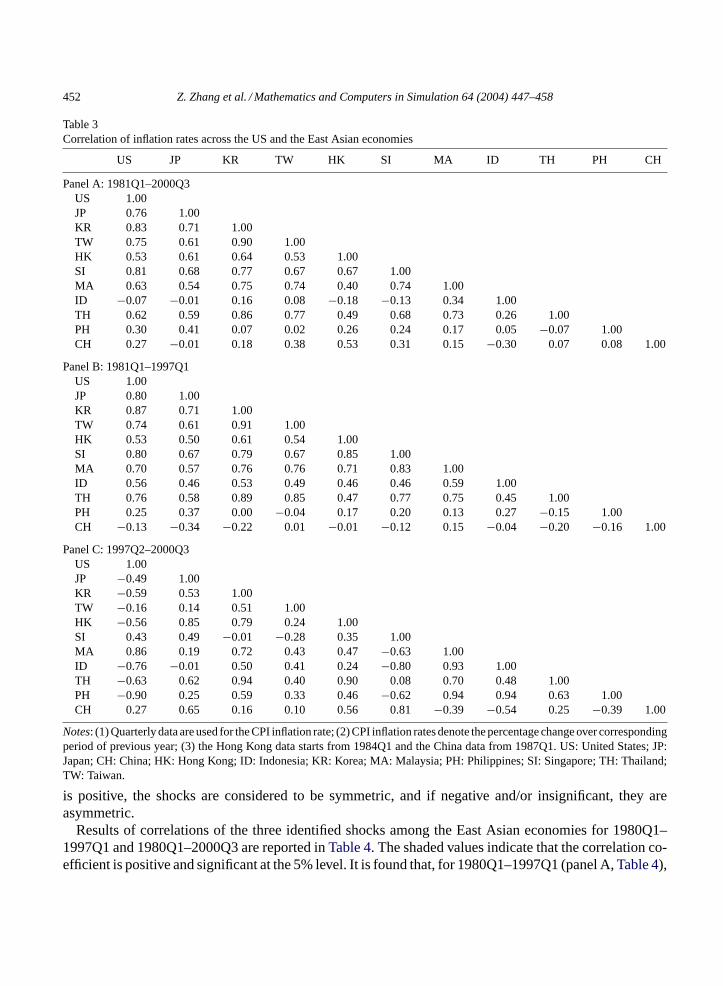
We now turn to the examination of the correlations in growth and inflation of the East Asian economiesfor specified periods (seeTables 2 and 3).2 Overall, the East Asian economies display a less obviouspattern in GDP growth compared with inflationary movements, even though the former has become morecorrelated after the financial crisis. It is interesting to note that the recent financial crisis has changed thecorrelation patterns of economic growth and inflation among the economies concerned. After the crisis,the number of significant correlations in GDP growth has increased among the East Asian countries,and between the US and the region. However, the financial crisis has changed a number of significantand positive correlations in inflation to insignificant and negative. These findings have implications forforming an OCA in the East Asian region.

2 In Tables 2 and 3, GDP growth rates and CPI inflation rates are calculated as a percentage change over the correspondingperiod in the previous year.


Table 2Correlation of GDP growth rates across the US and the East Asian economies

US JP KR TW HK SI MA ID TH PH CH

Panel A: 1981Q1–2000Q3US 1.00JP −0.06 1.00KR −0.03 0.44 1.00TW 0.38 0.27 0.45 1.00HK 0.21 0.25 0.63 0.68 1.00SI 0.00 0.17 0.34 0.22 0.52 1.00MA −0.10 0.28 0.54 0.07 0.45 0.75 1.00ID −0.03 0.43 0.65 0.31 0.58 0.54 0.79 1.00TH −0.16 0.57 0.70 0.26 0.45 0.53 0.70 0.77 1.00PH −0.20 0.04 0.12 −0.10 0.14 0.40 0.35 0.20 0.22 1.00CH 0.27 −0.01 0.11 0.25 0.17 −0.11 −0.11 0.10 0.08 −0.54 1.00

Panel B: 1981Q1–1997Q1US 1.00JP 0.09 1.00KR 0.07 0.20 1.00TW 0.50 0.12 0.53 1.00HK 0.31 0.00 0.41 0.73 1.00SI 0.04 −0.05 0.01 0.11 0.35 1.00MA −0.06 −0.08 −0.13 −0.20 0.02 0.70 1.00ID 0.30 −0.10 −0.17 0.09 0.23 0.35 0.50 1.00TH −0.04 0.30 0.14 0.07 0.04 0.50 0.47 0.22 1.00PH −0.25 0.06 0.00 −0.12 0.05 0.38 0.36 0.23 0.37 1.00CH 0.41 −0.26 −0.02 0.16 0.11 −0.24 −0.37 −0.36 −0.33 −0.57 1.00

Panel C: 1997Q2–2000Q3US 1.00JP 0.24 1.00KR 0.46 0.72 1.00TW 0.17 0.52 0.48 1.00HK 0.68 0.70 0.84 0.69 1.00SI 0.47 0.65 0.77 0.80 0.91 1.00MA 0.46 0.73 0.91 0.72 0.93 0.93 1.00ID 0.44 0.61 0.85 0.74 0.90 0.95 0.97 1.00TH 0.60 0.60 0.96 0.30 0.81 0.68 0.83 0.77 1.00PH 0.35 0.55 0.80 0.70 0.84 0.92 0.92 0.97 0.72 1.00CH −0.08 −0.08 −0.17 −0.11 −0.01 0.03 −0.15 −0.06 −0.12 0.03 1.00

Notes: (1) Quarterly data are used for the real GDP growth rate; (2) GDP growth rates denote the percentage change overcorresponding period of previous year. US: United States; JP: Japan; CH: China; HK: Hong Kong; ID: Indonesia; KR: Korea;MA: Malaysia; PH: Philippines; SI: Singapore; TH: Thailand; TW: Taiwan.

3.3. Correlation of structural shocks

The underlying shocks were estimated by the structural VAR approach for the East Asian economiesfor 1980Q1–1997Q1 and 1980Q1–2000Q3. It is assumed that if the correlation of structural shocks


Table 3Correlation of inflation rates across the US and the East Asian economies

US JP KR TW HK SI MA ID TH PH CH

Panel A: 1981Q1–2000Q3US 1.00JP 0.76 1.00KR 0.83 0.71 1.00TW 0.75 0.61 0.90 1.00HK 0.53 0.61 0.64 0.53 1.00SI 0.81 0.68 0.77 0.67 0.67 1.00MA 0.63 0.54 0.75 0.74 0.40 0.74 1.00ID −0.07 −0.01 0.16 0.08 −0.18 −0.13 0.34 1.00TH 0.62 0.59 0.86 0.77 0.49 0.68 0.73 0.26 1.00PH 0.30 0.41 0.07 0.02 0.26 0.24 0.17 0.05 −0.07 1.00CH 0.27 −0.01 0.18 0.38 0.53 0.31 0.15 −0.30 0.07 0.08 1.00

Panel B: 1981Q1–1997Q1US 1.00JP 0.80 1.00KR 0.87 0.71 1.00TW 0.74 0.61 0.91 1.00HK 0.53 0.50 0.61 0.54 1.00SI 0.80 0.67 0.79 0.67 0.85 1.00MA 0.70 0.57 0.76 0.76 0.71 0.83 1.00ID 0.56 0.46 0.53 0.49 0.46 0.46 0.59 1.00TH 0.76 0.58 0.89 0.85 0.47 0.77 0.75 0.45 1.00PH 0.25 0.37 0.00 −0.04 0.17 0.20 0.13 0.27 −0.15 1.00CH −0.13 −0.34 −0.22 0.01 −0.01 −0.12 0.15 −0.04 −0.20 −0.16 1.00

Panel C: 1997Q2–2000Q3US 1.00JP −0.49 1.00KR −0.59 0.53 1.00TW −0.16 0.14 0.51 1.00HK −0.56 0.85 0.79 0.24 1.00SI 0.43 0.49 −0.01 −0.28 0.35 1.00MA 0.86 0.19 0.72 0.43 0.47 −0.63 1.00ID −0.76 −0.01 0.50 0.41 0.24 −0.80 0.93 1.00TH −0.63 0.62 0.94 0.40 0.90 0.08 0.70 0.48 1.00PH −0.90 0.25 0.59 0.33 0.46 −0.62 0.94 0.94 0.63 1.00CH 0.27 0.65 0.16 0.10 0.56 0.81 −0.39 −0.54 0.25 −0.39 1.00

Notes: (1) Quarterly data are used for the CPI inflation rate; (2) CPI inflation rates denote the percentage change over correspondingperiod of previous year; (3) the Hong Kong data starts from 1984Q1 and the China data from 1987Q1. US: United States; JP:Japan; CH: China; HK: Hong Kong; ID: Indonesia; KR: Korea; MA: Malaysia; PH: Philippines; SI: Singapore; TH: Thailand;TW: Taiwan.

is positive, the shocks are considered to be symmetric, and if negative and/or insignificant, they areasymmetric.

Results of correlations of the three identified shocks among the East Asian economies for 1980Q1–1997Q1 and 1980Q1–2000Q3 are reported inTable 4. The shaded values indicate that the correlation co-efficient is positive and significant at the 5% level. It is found that, for 1980Q1–1997Q1 (panel A,Table 4),


Table 4Correlation of structural shocks across the East Asian economies

J p Kr Tw HK Si Ml Id Th Ph Ch J p Kr Tw HK Si Ml Id Th Ph Ch

Panel A: S upply S hock s (1980Q3-1997Q1) Panel D: S upply S hock s (1980Q3-2000Q3)J apan 1.00 1.00

Korea 0.22 1.00 0.32 1.00

Taiwan 0.28 0.48 1.00 0.33 0.40 1.00

Hong Kong 0.27 0.18 0.47 1.00 0.25 0.34 0.49 1.00

Singapore 0.07 0.19 0.31 0.10 1.00 0.20 0.29 0.42 0.20 1.00

Malaysia 0.27 0.27 0.22 -0.01 0.45 1.00 0.36 0.53 0.30 0.13 0.51 1.00

Indonesia 0.08 0.24 0.18 -0.14 0.23 0.45 1.00 0.27 0.50 0.37 0.15 0.38 0.50 1.00

Thailand 0.08 0.34 0.20 -0.02 0.25 0.27 0.28 1.00 0.13 0.40 0.19 0.05 0.26 0.42 0.35 1.00

Ph ilippines 0.32 0.23 0.21 0.32 0.20 0.22 0.11 0.06 1.00 0.27 0.25 0.19 0.31 0.22 0.24 0.21 0.11 1.00

China 0.00 0.03 0.23 0.25 0.20 0.17 0.14 -0.09 0.13 1.00 0.15 0.17 0.29 0.27 0.26 0.20 0.27 0.14 0.20 1.00

Panel B: Dem and S hock s (1980Q3-1997Q1) Panel E: Dem and S hock s (1980Q3-2000Q3)J apan 1.00 1.00

Korea 0.23 1.00 0.03 1.00

Taiwan 0.26 0.42 1.00 0.41 0.43 1.00

Hong Kong -0.09 0.27 0.00 1.00 -0.11 0.21 -0.19 1.00

Singapore 0.44 0.16 0.24 0.18 1.00 0.57 0.22 0.47 0.02 1.00

Malaysia 0.28 0.01 0.07 0.20 0.58 1.00 0.15 0.37 0.37 0.09 0.50 1.00

Indonesia 0.20 0.19 0.02 0.03 0.13 0.03 1.00 0.16 0.42 0.31 -0.07 0.27 0.27 1.00

Thailand 0.40 -0.06 0.07 -0.09 0.27 0.36 -0.04 1.00 0.09 0.27 0.19 0.05 0.20 0.43 0.07 1.00

Ph ilippines -0.01 0.23 0.19 0.15 0.08 0.05 0.00 0.00 1.00 0.00 0.30 0.27 0.08 0.18 0.15 0.11 0.13 1.00

China -0.08 0.10 -0.12 0.11 -0.25 0.23 0.12 -0.11 0.21 1.00 -0.14 0.21 -0.05 0.03 -0.15 0.17 0.00 0.01 0.20 1.00

Panel C: Monetary S hock s (1980Q3-1997Q1) Panel F: Monetary S hock s (1980Q3-2000Q3)J apan 1.00 1.00

Korea 0.06 1.00 0.02 1.00

Taiwan 0.07 0.23 1.00 0.12 0.25 1.00

Hong Kong 0.13 0.09 0.10 1.00 0.00 -0.05 -0.04 1.00

Singapore 0.25 0.22 -0.02 -0.02 1.00 0.22 0.21 -0.01 -0.24 1.00

Malaysia 0.15 0.24 0.14 -0.04 0.55 1.00 0.16 0.30 0.16 -0.18 0.52 1.00

Indonesia 0.11 0.24 0.19 -0.16 0.16 0.35 1.00 0.03 0.26 0.25 0.01 0.22 0.37 1.00

Thailand 0.32 0.18 0.09 0.49 0.29 0.19 -0.12 1.00 0.36 0.19 0.11 0.38 0.23 0.24 0.25 1.00

Ph ilippines -0.01 -0.15 0.04 0.29 -0.08 -0.16 -0.01 -0.03 1.00 0.00 -0.01 0.10 0.22 0.11 -0.04 0.18 0.09 1.00

China -0.24 0.33 -0.02 0.06 0.12 0.53 0.15 0.07 -0.23 1.00 -0.26 0.32 -0.07 0.21 0.03 0.27 0.08 0.19 -0.10 1.00

Notes: The sample period starts from 1983Q3 for Hong Kong and from 1986Q3 for China. The shaded values denote positiveand significant at the 5% level. Significance levels are assessed using the Fisher’s variance-stabilising transformation, and thenull hypothesis is that the correlation coefficient is zero[11].

supply shocks are correlated significantly among Singapore, Malaysia, Indonesia and Thailand. Japanand Korea are positively and significantly correlated with some ASEAN economies. Correlations are alsohigh among Japan, Korea, Taiwan and Hong Kong. This result is similar to those in[2]. However, demandshocks and monetary shocks are less correlated among these economies during the sample period (panelsB and C,Table 4).

It is interesting to note that the regional financial crisis improved the number of significant correlationsof shocks in these economies (panels D–F,Table 4). Those ASEAN economies and NIEs that displayedhigh correlations in their growth patterns are likely to have similar supply shocks, which tend to bepermanent. For the rest of East Asia, asymmetric shocks seem to prevail. However, one should be cautiousas including the post-crisis period in the sample may cause structural breaks in the series, which wouldaffect estimation.3

3 The underlying shocks have been estimated by the structural VAR approach using data from the 1980s and 1990s prior tothe financial crisis. The number of significant correlations of the three identified shocks among the East Asian economies in the1990s do not change as much in the 1980s.


According to the OCA literature, supply shocks are considered to be more informative for evaluatingthe symmetry of shocks because estimated demand and monetary shocks using the structural VAR methodtend to include the effects of macroeconomic policies, as well as purely stochastic disturbances[2,5,6].The more (less) often are symmetric shocks encountered, the greater (lesser) are the correlations in thesupply shocks, and the more feasible does it become for these economies to establish an OCA. Therefore,our results do not display strong support for forming an OCA in the entire East Asian region. However,they do suggest that the OCA is feasible in some sub-regions, such as among some Asian NIEs andASEAN countries.

3.4. Variance decomposition analysis

Variance decomposition analysis is performed to identify the contribution of each shock to the threevariables. We decompose variation in the percentage change of the forecast error variance of changes inreal output, exchange rates and prices that are due to each shock at the 1–20-quarter horizons. Due tospace limitations,Table 5reports the VD results of real exchange rates, output and prices at the 1- and20-quarter horizons only (the remaining results are available on request).

In both sample periods, supply shocks are found to be the predominant shocks accounting for thevariability of real output in all East Asian economies. The supply shocks account for over 85% of thevariability at all horizons for the sample period prior to the crisis, and 64% when the post-crisis period isincluded. It is interesting to note that the financial crisis has reduced the influence of the supply shockson real output in most East Asian economies, but has increased the influence in Japan. The economieshardest hit by the recent financial crisis displayed an increasing effect of demand and monetary shockson real output.

In contrast to real output, monetary shocks in both sample periods are the predominant shocks forthe variability of the price level for all East Asian economies, except for Hong Kong and Philippines.The demand shocks predominate in Hong Kong and Philippines, accounting for over 50 and 85%, re-spectively. By accommodating the financial crisis, these effects have become enhanced substantially inHong Kong, but become weakened in Philippines. By including the post-crisis period, supply shocks be-come the predominant shocks after a 2-quarter horizon in Indonesia, and are not influential in the rest ofEast Asia.

Fluctuations in real exchange rates were predominantly caused by the demand shocks at all horizons forall East Asian economies before the financial crisis. The crisis has changed the effects of demand shocks,especially in the economies hardest hit by the crisis. Supply shocks became the predominant cause ofthe variability in real exchange rates after the crisis in Indonesia, Korea and Thailand, and remain strongfor all horizons. This finding has important policy implications for the exchange rate regimes in thesecountries.

3.5. Impulse response function analysis

Since the estimated structural shocks are assumed to have unit variances in the structural VAR, theirsize and adjustment speed can be inferred by analysing the associated impulse response functions (see[2]). For the size of supply shocks, the long run (20-quarter horizon) effect of a unit shock on changes inreal GDP is used. For demand and monetary shocks, the 1-quarter impact on changes in real exchangerates and CPI is chosen as a measure of size. The speed of adjustment is measured as the share of the


Table 5Variance decomposition of the changes in output, exchange rate and price

Real output Real exchange rate Price

Supplyshock

Demandshock

Monetaryshock

Supplyshock

Demandshock

Monetaryshock

Supplyshock

Demandshock

Monetaryshock

Panel A: 1980Q3–1997Q1JP 95.5/94.3 4.5/5.7 0.0/0.1 15.3/14.1 84.1/84.6 0.6/1.2 3.5/3.3 1.3/1.1 95.2/95.6KR 95.4/93.0 0.1/0.2 4.5/6.9 3.5/16.0 90.3/80.2 6.2/3.8 5.5/5.1 7.5/7.0 87.0/87.8TW 99.1/98.9 0.0/0.0 0.9/1.1 3.4/14.2 87.2/78.1 9.5/7.7 1.6/2.6 9.3/8.9 89.0/88.5HK 98.4/97.4 0.4/0.9 1.2/1.7 0.0/0.5 98.8/98.6 1.1/0.9 1.7/2.5 52.8/48.8 45.5/48.7SI 93.4/90.0 3.1/3.7 3.5/6.3 11.0/10.1 82.0/78.7 7.0/11.2 1.6/4.0 25.8/25.1 72.6/71.0MA 96.2/93.9 0.4/0.5 3.4/5.5 0.2/2.7 99.7/97.2 0.1/0.1 3.1/6.2 5.8/9.9 91.2/83.9ID 91.7/85.6 5.5/10.3 2.7/4.1 13.7/14.9 80.4/75.4 5.8/9.7 3.4/3.4 2.4/2.5 94.2/94.0TH 99.1/98.6 0.0/0.2 0.8/1.2 2.1/2.3 97.3/96.9 0.6/0.8 0.2/0.3 21.8/22.5 78.0/77.2PH 92.3/89.7 1.2/1.8 6.5/8.5 3.2/3.6 96.8/96.3 0.0/0.1 0.0/3.4 89.0/84.9 11.0/11.7CH 96.8/93.5 2.1/3.0 1.1/3.5 0.2/3.9 69.7/61.6 30.1/34.5 1.0/1.0 34.5/34.5 64.5/64.6

Panel B: 1980Q3–2000Q3JP 99.9/99.8 0.1/0.1 0.1/0.1 5.5/5.3 93.9/93.6 0.6/1.1 8.4/8.6 2.8/4.0 88.8/87.4KR 80.2/72.1 18.0/23.5 1.8/4.3 54.1/48.8 42.8/47.6 3.1/3.6 8.7/7.9 3.5/7.3 87.7/84.7TW 96.8/95.7 2.7/3.4 0.5/0.9 5.2/13.8 88.0/80.0 6.8/6.2 0.9/1.7 11.1/10.7 88.0/87.6HK 98.8/98.6 0.5/0.6 0.7/0.7 0.0/2.3 83.6/87.7 16.4/10.0 0.7/3.6 88.7/78.4 10.6/18.1SI 91.2/88.8 6.3/7.4 2.5/3.8 14.8/14.9 83.4/82.2 1.8/2.9 0.8/4.0 7.4/7.3 91.8/88.7MA 70.7/70.6 29.1/29.1 0.2/0.2 31.8/29.3 68.2/70.7 0.0/0.0 0.2/0.9 1.4/3.7 98.4/95.4ID 63.7/69.0 20.7/11.9 15.6/19.1 62.5/59.8 21.0/21.5 16.5/18.7 21.8/58.4 13.0/7.9 65.2/33.7TH 70.7/76.2 17.8/14.1 11.5/9.6 39.4/39.0 60.4/60.6 0.2/0.3 7.1/15.0 3.7/6.5 89.3/78.5PH 87.4/83.6 3.2/4.3 9.4/12.1 4.8/5.1 94.6/93.8 0.6/1.1 0.0/3.2 79.8/76.8 20.2/20.1CH 92.3/87.5 0.4/0.6 7.3/11.9 1.3/6.6 81.5/72.7 17.2/20.7 9.1/12.8 24.6/22.6 66.3/64.5

Notes: The values indicate the percentage change of the forecast error variance in the real exchange rate, output and pricethat is due to each shock at the 1- and 20-quarter horizons. The data is given as the VD results of the corresponding shock atthe 1-/20-quarter horizons. The sample period starts from 1983Q3 for Hong Kong and from 1986Q3 for China. JP: Japan;CH: China; HK: Hong Kong; ID: Indonesia; KR: Korea; MA: Malaysia; PH: Philippines; SI: Singapore; TH: Thailand;TW: Taiwan.

response after 4-quarters in its long run effect (that is, the response after a 20-quarter horizon).4 The largeris the size of the shocks, the more disruptive will be the effects on an economy. Similarly, the slower isthe adjustment to disturbances, the larger will be the cost of maintaining a fixed exchange rate system.Table 6reports the size of shocks and the speed of adjustments to shocks.

The dynamic impulse responses of real output and exchange rates with respect to the identified shocksare consistent with the results using variance decomposition analysis. As seen inTable 6, the size ofthe supply shocks is the largest in the most open economies, such as Singapore, Hong Kong, Malaysia,Thailand and Philippines. For demand and monetary shocks, China, Indonesia and Philippines havethe biggest sizes. The recent financial crisis has, in general, increased the size of disturbances. As a

4 Our choice of the time horizon in calculating the size of shocks and the speed of adjustment is somewhat arbitrary. However,choosing different horizons as a measure will not change the conclusion.


Table 6Size of shocks and speed of adjustment to shocks

Supply shocks Demand shocks Monetary shocks

Size Speed Size Speed Size Speed

Panel A: 1980Q3–1997Q1JP 0.013 0.999 0.051 0.997 0.006 0.981KR 0.015 0.977 0.014 0.734 0.009 0.966TW 0.012 1.000 0.019 0.920 0.011 0.981HK 0.021 1.000 0.010 0.937 0.005 0.989SI 0.020 0.994 0.018 0.997 0.005 0.998MA 0.020 0.989 0.023 0.993 0.007 0.995ID 0.012 0.999 0.045 0.999 0.013 1.000TH 0.019 0.998 0.023 0.990 0.007 0.999PH 0.027 0.984 0.116 1.001 0.036 0.960CH 0.016 1.000 0.055 0.987 0.021 0.984

Average 0.018 0.994 0.037 0.956 0.012 0.985

Panel B: 1980Q3–2000Q3JP 0.014 1.000 0.055 0.996 0.006 0.991KR 0.022 1.002 0.031 1.008 0.010 1.006TW 0.013 0.983 0.023 0.921 0.010 0.974HK 0.025 0.991 0.009 0.765 0.003 0.675SI 0.022 0.990 0.021 0.996 0.006 1.000MA 0.026 0.996 0.029 1.001 0.008 0.999ID 0.030 1.065 0.048 1.093 0.019 1.085TH 0.033 0.939 0.036 0.997 0.008 0.990PH 0.025 0.984 0.107 1.000 0.045 0.970CH 0.016 1.000 0.053 0.996 0.020 0.986

Average 0.022 0.995 0.041 0.977 0.013 0.968

JP: Japan; CH: China; HK: Hong Kong; ID: Indonesia; KR: Korea; MA: Malaysia; PH: Philippines; SI: Singapore; TH: Thailand;TW: Taiwan.

comparison, the average size of the supply shocks in East Asia is almost double that of 14 Europeancountries for a similar time period (see[13]).

However, the speed of adjustment to disturbances in East Asia is much faster than in Europe. Most ofthe East Asian countries take less than 1 year to complete the adjustment to shocks. The pace becameeven more rapid during the financial crisis. One possible explanation is that the labour market in mostEast Asian countries is very flexible, so that it is much easier for these economies to adjust internally inresponse to shocks.5 These findings support the proposal for a common currency arrangement. Accordingto the OCA literature, countries are better candidates for a currency arrangement if their disturbances arecorrelated and small, and if these countries adjust rapidly to shocks.

5 One of the popular measures used in these economies during the financial crisis was to freeze or cut salaries to reduce labourcosts and maintain their competitiveness. This measure would possibly be difficult to implement in countries with strong labourunions.


4. Concluding remarks

This paper used a three-variable VAR model to identify various types of shocks, using more than twodecades of quarterly data from East Asia. The results showed that the exchange rates of the East Asianeconomies are relatively stable. However, these economies display a less coherent pattern in GDP growththan that of inflation, though the former has become more correlated after the financial crisis. Prior to therecent financial crisis, supply shocks were correlated significantly among some ASEAN countries (suchas Singapore, Malaysia, Indonesia and Thailand) and East Asian countries (such as Hong Kong, Japan,Korea and Taiwan). This result is similar to the findings in[2]. However, demand shocks and monetaryshocks were less correlated among these economies during the sample period.

It is interesting to note that the regional financial crisis improved the number of significant correlations ofshocks in these economies. Those economies that displayed high correlations in their growth patterns werelikely to have similar supply shocks, which tend to be permanent. For the rest of East Asia, asymmetricshocks seem to prevail. According to the OCA literature, supply shocks are considered to be moreinformative for evaluating the symmetry of shocks. The greater (lesser) are the symmetric shocks thatthe economies encounter, the higher (lower) are the correlations in supply shocks, and the more feasibledoes it become for these economies to establish an OCA.

The results from VD analysis show that the supply shocks in the two sample periods are the predominantshocks for the variability of real output in all the East Asian economies. Interestingly the financial crisis hasreduced the influence of the supply shocks on real output in most East Asian economies, but has increasedthe influence in Japan. The economies most hit by the financial crisis displayed an increasing effect of thedemand and monetary shocks on real output. In contrast, monetary shocks are the predominant shocks forthe variability of the price level for all East Asian economies, except for Hong Kong and Philippines. Forthe latter, demand shocks are predominant for all horizons. By including the post-crisis period, supplyshocks become the predominant shocks after a two-quarter horizon only in Indonesia. The fluctuationsin real exchange rates were predominantly caused by the demand shocks for all horizons in East Asiaeconomies before the financial crisis. Those economies hardest hit by the financial crisis show that thesupply shocks become the predominant cause of the variability in real exchange rates after the crisis, andsuch effects remain strong for all horizons. This has important policy implications for the exchange rateregimes in these countries.

The dynamic impulse responses of real output and exchange rates with respect to the identified shocksare consistent with the results using VD analysis. Although the size of the underlying shocks is largerthan in Europe, the speed of adjustments to shocks in East Asia is much faster, taking less than 1 year inmost countries. It is clear that the flexible labour markets in these economies have facilitated the internaladjustment process.

Overall, the empirical results do not display strong support for forming an optimum currency area inthe East Asian region. However, they do imply that some sub-regions are better candidates for a currencyarrangement as their disturbances are correlated and small, and these countries adjust rapidly to shocks.

Acknowledgements

The authors wish to thank Paul De Grauwe, Harry Bloch, Ian Kerr, Ken Clements, Mansur Masih,Edward Lim, Sadayuki Takii, conference participants at MODSIM in Canberra, and seminar participants


at the International Centre for the Study of East Asian Development (ICSEAD), University of WesternAustralia, Curtin University and Edith Cowan University, for helpful comments and suggestions. Thisstudy was begun while the first author was visiting ICSEAD, Japan. He wishes to thank ICSEAD for itshospitality and support and UMAC for financial support through grant RG042/00-01S. The second andthird authors wish to acknowledge the financial support of ICSEAD and an Australian Research CouncilDiscovery Grant, respectively.

References

[1] T. Bayoumi, B. Eichengreen, Shocking aspects of European monetary integration, in: F. Torres, F. Giavazzi (Eds.),Adjustment and Growth in the European Monetary Union, Cambridge University Press, Cambridge, 1993, pp. 193–229.

[2] T. Bayoumi, B. Eichengreen, One Money or Many? Analyzing the Prospects for Monetary Unification in Various Parts of theWorld, Princeton Studies in International Finance, vol. 16, International Finance Section, Princeton University, Princeton,1994.

[3] O.J. Blanchard, D. Quah, The dynamic effects of aggregate demand and supply disturbances, Am. Econ. Rev. 79 (1989)655–673.

[4] R. Clarida, J. Gali, Sources of real exchange-rate fluctuations: how important are nominal shocks? Carnegie-RochesterConf. Ser. Public Policy 41 (1994) 1–56.

[5] M. Demertzis, A.H. Hallett, O. Rummel, Is the European Union a national currency area, or is it held together by policymakers, Weltwirtschaftliches Arch. 136 (2000) 657–679.

[6] M. Kawai, T. Okumura, Higashi Ajia ni okeru Makuro Keizai-teki Sougo Izon (Macro economic interdependence in theEast Asian region), in: M. Kawai (Ed.), Ajia no Kin-yu Shihon Shijo (Financial and Capital Markets in Asia), Nihon KeizaiShinbunsha, Tokyo, 1996, pp. 217–237 (in Japanese).

[7] R.I. McKinnon, Optimum currency areas, Am. Econ. Rev. 53 (1963) 717–725.[8] R.A. Mundell, A theory of optimum currency areas, Am. Econ. Rev. 51 (1961) 657–665.[9] K. Phylaktis, Capital market integration in the Pacific-Basin region: an analysis of real interest rate linkages, Pacific-Basin

Finance J. 5 (1997) 195–213.[10] K. Phylaktis, Capital market integration in the Pacific-Basin region: an impulse response analysis, J. Int. Money Finance

18 (1999) 267–287.[11] R.N. Rodriguez, Correlation, in: S. Kotz, N.L. Johnson (Eds.), Encyclopedia of Statistical Sciences, vol. 2, Wiley, New

York, 1982, pp. 193–204.[12] J.H. Rogers, Monetary shocks and real exchange rates, International Finance Discussion Paper no. 612, Board of Governors

of the Federal Reserve System, Washington, DC, 1998.[13] K. Sato, Z. Zhang, M. McAleer, Is East Asia an optimum currency area?, paper presented at the 2001 Far Eastern Meeting

of the Econometric Society, Kobe, Japan, 20–22 July 2001.

asian monetary integration: a structural var approach

Documents