aspatiallyexplicitmodellingframeworkforassessing ... · inra igepp, biosp & eco-innov units...
TRANSCRIPT

Context Landscape simulations Pollen dispersal Spatial risk evaluation Sensitivity analysis Further development Conclusion
A spatially explicit modelling framework for assessingecotoxicological risks at the landscape scale
Melen Leclerc, Emily Walker, Antoine Messéan and Samuel Soubeyrand
INRA IGEPP, BioSP & Eco-Innov units
25/05/2016 - SSIAB - Rennes
Context Landscape simulations Pollen dispersal Spatial risk evaluation Sensitivity analysis Further development Conclusion
Context
Risk assessment is the determination of quantitative or qualitativeestimate of risk related to a concrete situation and a recognized hazard
We consider the consequences of pollution or contaminant spread on theenvironment and exposed populations
Modelling approaches are needed for quantifying risk and testingmanagement strategies
Considering large spatial scales is often crucial for Environmental andecological risk assessment

Context Landscape simulations Pollen dispersal Spatial risk evaluation Sensitivity analysis Further development Conclusion
The impact of GM crops on non-target organisms
Bt crops are GM plants producing insecticidal proteins
Bt toxins are also expressed in pollen that spread outside fields and canreach habitats of non-target organisms (NTOs)
GM crops can have ecological impacts on populations withinagroecosystems
Need of spatial models at the landscape scale for risk assessment and forbuilding management strategies
In the study we consider the impacts of Bt maize MON810 on the peacockbutterfly (which lay eggs on nettle plants)

Context Landscape simulations Pollen dispersal Spatial risk evaluation Sensitivity analysis Further development Conclusion
How to structure simplified agriculturallandscapes ?
Ingredients:
→ Convexe fields
→ GM and non-GM fields
→ Field margins with host-plants
Control:
→ The number of fields I
→ The mean thickness of host-margins u
→ The proportion of GM fields p
→ Spatial aggregation of GM fields
→ Location of host-margins with respect to GM fields

Context Landscape simulations Pollen dispersal Spatial risk evaluation Sensitivity analysis Further development Conclusion
Structuration of the landscape
The landscape is structured by:
1 Simulating a binomial point process X = x1, . . . , xI of I points inΩ = 5000× 5000m2
2 Drawing a Vornoi tessellation Θ in order to partition Ω from X as seedpoints
Context Landscape simulations Pollen dispersal Spatial risk evaluation Sensitivity analysis Further development Conclusion
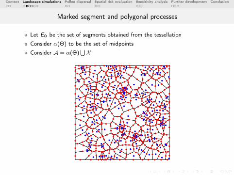
Marked segment and polygonal processes
Let EΘ be the set of segments obtained from the tessellation
Consider α(Θ) to be the set of midpoints
Consider A = α(Θ)⋃X
Context Landscape simulations Pollen dispersal Spatial risk evaluation Sensitivity analysis Further development Conclusion
Marked segment and polygonal processes
Consider a Gaussian stationary spatial process Λ with a Matérnautocovariance function
σ2 1Γ(ν)2ν−1
(√2ν‖xj − xk‖
ρ
)νKν(√
2ν‖xj − xk‖
ρ
)
Then for each x ∈ A, we draw Λ(x1), . . . ,Λ(xN) ∼ N (µ, . . . , µ),Σ
We fix σ = 1, ν = 5, and, µ = 0
We keep the range parameter ρ

Context Landscape simulations Pollen dispersal Spatial risk evaluation Sensitivity analysis Further development Conclusion
Attaching marks by thresholding the GP
Field-polygons
Xm =X = x1, . . . , xI; mX = e (emitting); o (other)
→ Let nc = bpc Ic be the number of GM fields→ Consider the threshold sX = Λnc (xk) that is the nc iest drawn value
mX (xi ) = e if Λ(xi ) ≤ sXmX (xi ) = o if Λ(xi ) > sX
Margin-segments
α(Θ)m =α(Θ) = x1, . . . , xN; mα(Θ) = n (neutral); h (host)
→ As we want to control the locations of margins with respect to GM fields
α(Θ)m is built from Xmmα(Θ)(xk) = h if (sX + τ − δ) < Λ(xk) < (sX + τ + δ)
else mα(Θ)(xk) = n
τ is kept as a parameter and we fix δ = 0.1

Context Landscape simulations Pollen dispersal Spatial risk evaluation Sensitivity analysis Further development Conclusion
Adding thickness to host segments
Let EΘm(h) =e1, . . . , eNh
be the set of host-margin segments. A
thickness εn ≥ 0 is associated to each host segment en (n = 1, . . . ,Nh).The thicknesses are identically and independently drawn from a Gammadistribution (mean = u,variance = 4)
Then, for each n ∈ 1, . . . ,N1, the dilated segments ed,n are obtained byen 7→ en
⊕Bn where B is a sphere with diameter εn/2
M =
Nh⋃n=1
en⊕
Bn

Context Landscape simulations Pollen dispersal Spatial risk evaluation Sensitivity analysis Further development Conclusion
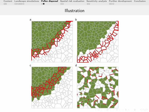
Illustration
a b
c d

Context Landscape simulations Pollen dispersal Spatial risk evaluation Sensitivity analysis Further development Conclusion
Simulation of pollen spread and drop-off
The amount of pollen grains located at position (x , y) is obtained bycalculating the convolution product between the emission E(x , y) and adispersal kernel K
Ra(x , y) =
∫ ∫E(x ′, y ′)K(x − x ′, y − y ′)dx ′dy ′ = E ⊗ K(x , y)
,
R(x , y) = Ra(x , t) ∗ adherence ∗ (1− loss) = Ra(x , y) ω (1− ψ)
Four dispersal kernels are used (isotropic and anistotropic Normal InverseGaussian, Geometric and bivariate Student kernels)
The convolution product was calculated by using Fast Fourier Transforms(FFT) and periodic boundary conditions
Context Landscape simulations Pollen dispersal Spatial risk evaluation Sensitivity analysis Further development Conclusion
Illustration
a b
c d

Context Landscape simulations Pollen dispersal Spatial risk evaluation Sensitivity analysis Further development Conclusion
Illustration
a b
c d
−2
0
2
4
6
8

Context Landscape simulations Pollen dispersal Spatial risk evaluation Sensitivity analysis Further development Conclusion
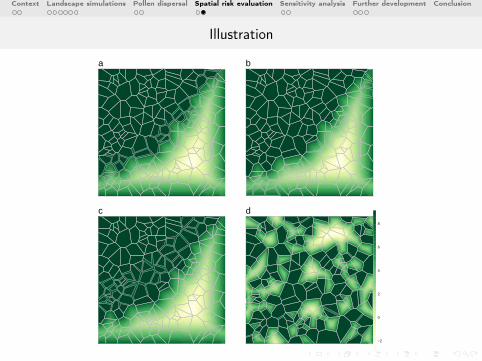
Assessing individual risk within the landscape
A risk map is obtained by using the following empirical dose-mortalityrelationship
→Pdeath =
e−9.304+2.473 log10(D)
1 + e−9.304+2.473 log10(D)
The locations of non-target individuals are simulated by drawing ahomogeneous binomial point process on host-margins
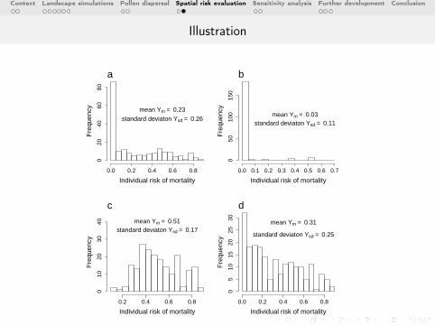
By assessing the risk for each individual we get a distribution of theindividual risk for the landscape
We extract the mean Ym and the standard deviation Ysd of thedistribution
Context Landscape simulations Pollen dispersal Spatial risk evaluation Sensitivity analysis Further development Conclusion
Illustration
a b
c d
−2
0
2
4
6
8

Context Landscape simulations Pollen dispersal Spatial risk evaluation Sensitivity analysis Further development Conclusion
Illustration
a
b
c
d
0.0
0.2
0.4
0.6
0.8
Context Landscape simulations Pollen dispersal Spatial risk evaluation Sensitivity analysis Further development Conclusion
Illustration
Individual risk of mortality
Fre
quen
cy
0.0 0.2 0.4 0.6 0.8
020
4060
80
mean Ym = 0.23
standard deviaton Ysd = 0.26
a
Individual risk of mortality
Fre
quen
cy
0.0 0.1 0.2 0.3 0.4 0.5 0.6 0.7
050
100
150
mean Ym = 0.03standard deviaton Ysd = 0.11
b
Individual risk of mortality
Fre
quen
cy
0.2 0.4 0.6 0.8
010
2030
40 mean Ym = 0.51standard deviaton Ysd = 0.17
c
Individual risk of mortality
Fre
quen
cy
0.0 0.2 0.4 0.6 0.8
05
1015
2025
30 mean Ym = 0.31
standard deviaton Ysd = 0.25
d

Context Landscape simulations Pollen dispersal Spatial risk evaluation Sensitivity analysis Further development Conclusion
Sensitivity Analysis: assessing the influence of parameters onf the risk
Optimized Latin Hypercube Sampling (1000 points) with 10 replicates foreach point (stochastic model)Sensibility indices are obtained by using a metamodel (GLM) for Ym andYsd
0.3 0.4 0.5 0.6 0.7 0.8 0.90.0
1.0
2.0
Proportion of GM fields p
a)
0.2 0.4 0.6 0.8
0.0
1.0
Pollen loss ψ
b)
0 5 10 15 20 25 30
0.0
00
0.0
20
Margin mean thickness w
c)
0.0e+00 1.0e+07 2.0e+070e+
00
6e−
08
Emitted Pollen Ep
d)
0.30 0.40 0.50 0.60
0.0
1.5
3.0
Adherence on leaves ω
e)
0 500 1500 2500
0.0
00
0.0
10
Range parameterρ
f)
100 200 300 400 5000.0
000
0.0
015
Number of plots I
g)
−0.15 −0.05 0.05 0.15
0.0
1.0
2.0
3.0
Location of host−margins τ
h)
Context Landscape simulations Pollen dispersal Spatial risk evaluation Sensitivity analysis Further development Conclusion
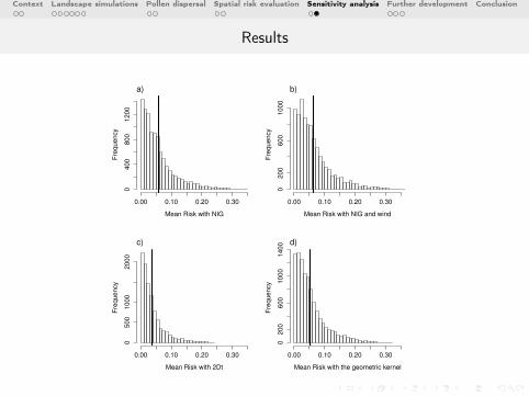
Results
Mean Risk with NIG
Fre
quency
0.00 0.10 0.20 0.30
0400
800
1200
a)
Mean Risk with NIG and wind
Fre
quency
0.00 0.10 0.20 0.30
0200
600
1000
b)
Mean Risk with 2Dt
Fre
quency
0.00 0.10 0.20 0.30
0500
1000
2000
c)
Mean Risk with the geometric kernel
Fre
quency
0.00 0.10 0.20 0.30
0200
600
1000
1400 d)

Context Landscape simulations Pollen dispersal Spatial risk evaluation Sensitivity analysis Further development Conclusion
Results
Em
ψ
ω
p
I
w
τ
ρ
K
Mean Risk Ym
0 5 10 20 30
a)
Em
ψ
ω
p
I
w
τ
ρ
K
Standard Deviation Ysd
0 5 10 15 20 25
b)

Context Landscape simulations Pollen dispersal Spatial risk evaluation Sensitivity analysis Further development Conclusion
Results

Context Landscape simulations Pollen dispersal Spatial risk evaluation Sensitivity analysis Further development Conclusion
Results
→ Substantial influence of pollen emission, spread anddrop-off (difficult to manage)
→ Significant influence of the spatial configuration of thelandscape
→ Landscape management may help in reducing the risk ofGM crops towards NTOs

Context Landscape simulations Pollen dispersal Spatial risk evaluation Sensitivity analysis Further development Conclusion
From spatial to spatio-temporal risk assessment
Emitting fields do not necessarily emit pollen at the same time
→ Emitted fields share the same discrete-time emission function E(t)
Ra(x , y , t) =
∫ ∫E(x ′, y ′, t)K(x − x ′, y − y ′)dx ′dy ′ = E ⊗ K(x , y , t)
→ The intensity of available contaminants R at site (x , y) and time t isdefined by
R(x , y , t) = 1− ψ(Z(t))R(x , y , t − 1) + ωRa(x , y , t)
Z is a time-varying positive covariate that linearly influences the lossfunction ψ (e.g. rain simulated by a stochastic weather generator)

Context Landscape simulations Pollen dispersal Spatial risk evaluation Sensitivity analysis Further development Conclusion
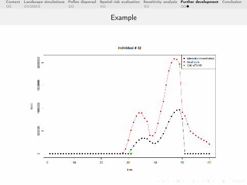
Toxicokinetic-toxicodynamic
The emipirial dose-mortality relationship does not represent well enoughthe toxicokinetic-toxicodynamic for exposed individual
→ We suppose that the individuals are affected by the contaminants with aconstant uptake rate kin > 0 and that they can eliminate contaminantsfrom their body at a constant elimination rate kout > 0
→ The internal concentration of contaminants within individual m,say ρm, isgiven by
dρm(t)
dt= kinR(zm, btc)− koutρm(t)
→ A lethal dose is fixed: when the internal concentration (ρ) of an individualreaches this threshold, the individual is considered dead
Larvae do not emerge at the same time
→ Individuals are represented by a marked point process with marksdescribing the time of emergence
Context Landscape simulations Pollen dispersal Spatial risk evaluation Sensitivity analysis Further development Conclusion
Example
Context Landscape simulations Pollen dispersal Spatial risk evaluation Sensitivity analysis Further development Conclusion
Conclusion
A generic and flexible modelling framework for assessing risks at largespatial scales
Implemented into the SEHmodel (Spatial Exposure-Hazard model) Rpackage
A toolbox for risk managers (European Food and Safety Authority) thatcan easily be expanded for various risk assessments and testingmanagement strategies
Stochastic geometry and spatial statistics provide interesting tools forsimulating simplified heterogeneous and fragmented environments (e.g.agricultural landscapes) and assessing their interactions with thespatio-temporal dynamics of populations
Studies that combined stochastic geometry-based environment simulators(e.g. landscape simulator) and population dynamics models often allowedecologists and epidemiologists to point out new management perspectives→ to be continued...

Context Landscape simulations Pollen dispersal Spatial risk evaluation Sensitivity analysis Further development Conclusion
Thank you for your attention