Aspects of Intersection Algorithms andApproximation

Tor Dokken

Revised January 2000

Submitted16. December 1996

tothe University of Oslo

for the doctor philosophiae degree.Defended July 1997

.Copyright: Tor Dokken, SINTEF ICT, Norway

e-mail: Tor.Dokken@sintef.no

Contents

1 Introduction 71.1 Intersection Algorithms Developed in Industrial Projects . . . 81.2 Relation to Trends . . . . . . . . . . . . . . . . . . . . . . . . 101.3 Why is Research on Intersection Algorithms Important? . . . 101.4 Summary . . . . . . . . . . . . . . . . . . . . . . . . . . . . . 111.5 Problems in Need of More Research . . . . . . . . . . . . . . . 12

2 A Generic Intersection Algorithm 142.1 Basic Concepts Used . . . . . . . . . . . . . . . . . . . . . . . 162.2 Geometric Tolerance and Intersection . . . . . . . . . . . . . . 182.3 Representation of the -Intersection . . . . . . . . . . . . . . . 212.4 Finding all Intersection Occurrences . . . . . . . . . . . . . . . 25

2.4.1 Spatial Separation with Respect to a Tolerance . . . . 262.4.2 Subdividing -Intersections into Disjoint Subsets . . . . 282.4.3 Subdivision at Points with Minimal Distance . . . . . . 292.4.4 Subdivision at Points with Maximal Distance . . . . . 302.4.5 Orientation of the Subdivision Borders . . . . . . . . . 332.4.6 Separating Connected Intersection Regions . . . . . . . 34

2.5 Loop Elimination . . . . . . . . . . . . . . . . . . . . . . . . . 342.5.1 The Set of Normals . . . . . . . . . . . . . . . . . . . . 352.5.2 Intersections Touching the Boundaries . . . . . . . . . 362.5.3 Boundary Subdivision Necessary . . . . . . . . . . . . 412.5.4 Finding Nonsingular Intersection Points . . . . . . . . 422.5.5 Combining Parametric and Algebraic Representations . 44

3 Representation of Geometric Objects 453.1 Parametric Representation of Closed and Bounded Manifolds. 453.2 The Algebraic Hypersurface . . . . . . . . . . . . . . . . . . . 52

1

4 Approximative Implicitization 544.1 Combining Parametric Manifolds and Algebraic Hypersurfaces 594.2 Stable Building of the D Matrix . . . . . . . . . . . . . . . . . 644.3 Implicitization by Singular Values . . . . . . . . . . . . . . . . 664.4 Constraining the Algebraic Equation . . . . . . . . . . . . . . 68

4.4.1 Interpolation of Position along a Manifold . . . . . . . 694.4.2 Interpolation of Tangent along a Manifold . . . . . . . 694.4.3 Interpolation of Normal along a Manifold . . . . . . . . 694.4.4 The Constraint Equation . . . . . . . . . . . . . . . . . 704.4.5 Direct Search for an Approximative Null Space . . . . 72

4.5 Convergence Rate of Approximative Implicitization . . . . . . 764.6 Accuracy of Approximative Implicitization . . . . . . . . . . . 81

4.6.1 Simple Direction for Error Measurement . . . . . . . . 824.7 Admissable Algebraic Approximations . . . . . . . . . . . . . 84

4.7.1 Normal Field of a Manifold . . . . . . . . . . . . . . . 854.7.2 Definition of Admissible Hypersurfaces . . . . . . . . . 89

4.8 Selecting an Approximative Implicitization . . . . . . . . . . . 904.9 Algorithm Approximative Implicitization . . . . . . . . . . . . 964.10 Approximative Implicitization of a Number of Manifolds . . . 974.11 Separating Manifolds Using Approximative Implicitization . . 994.12 Examples of Approximative Implicitization . . . . . . . . . . . 101

4.12.1 Example of 5th Degree Approximation . . . . . . . . . 1014.12.2 Example of 6th Degree Approximation . . . . . . . . . 1044.12.3 Example of 7th Degree Approximation . . . . . . . . . 104

5 Approximation of Intersection Results 1085.1 Intersection Representation within CAD . . . . . . . . . . . . 1095.2 Cubic Hermite Approximation of Intersection Results . . . . . 1115.3 Algebraic Approximation of Intersection Results . . . . . . . . 1125.4 Approximation of Algebraic Represented Manifolds . . . . . . 116

5.4.1 Approximating Manifolds Contained in an AlgebraicRepresented Hypersurface . . . . . . . . . . . . . . . . 119

5.4.2 Approximation of Manifolds in the Intersection of Al-gebraic Represented Hypersurfaces . . . . . . . . . . . 122

6 Cubic Hermite Approximation of 2D Curves 1276.1 Power Expansion Based on Parametric Representation . . . . 1286.2 Minimizing the Square Sum of the Coefficients . . . . . . . . . 1326.3 Cubic Hermite Approximation of Parametric Curves . . . . . . 134

2

7 Ellipse and Circle Approximation 1377.1 Taylor Expansion of Tangent Lengths . . . . . . . . . . . . . . 1397.2 Some Cubic Hermite Circle Interpolants . . . . . . . . . . . . 1477.3 Examples of Ellipse Approximations . . . . . . . . . . . . . . . 1597.4 Examples of Degree 4 Circle Approximation . . . . . . . . . . 164

A PosProd Basis Functions 179A.1 Tensor Product B-splines . . . . . . . . . . . . . . . . . . . . . 179A.2 Bernstein Bases over Simplices . . . . . . . . . . . . . . . . . . 180A.3 Tensor Product Bernstein Basis . . . . . . . . . . . . . . . . . 182

B Reformulation of Geometric Interrogations to Manifold In-tersections 185B.1 Intersection of Parametric Represented Manifolds and Hyper-

surfaces . . . . . . . . . . . . . . . . . . . . . . . . . . . . . . 186B.2 Finding Silhouette Curves in IR3 . . . . . . . . . . . . . . . . . 187

B.2.1 The normal vector . . . . . . . . . . . . . . . . . . . . 188B.2.2 Parallel Projection Silhouette in IR3 . . . . . . . . . . . 188B.2.3 Perspective Silhouette in IR3 . . . . . . . . . . . . . . . 188B.2.4 Circular Silhouette in IR3 . . . . . . . . . . . . . . . . . 189

B.3 Projection of a Manifold onto another Manifold . . . . . . . . 189B.3.1 Normal Projection . . . . . . . . . . . . . . . . . . . . 189B.3.2 Parallel Projection . . . . . . . . . . . . . . . . . . . . 190

B.4 Reformulation to extremal value problems. . . . . . . . . . . . 190

3

.

4

PrefaceMy work on intersection algorithms started in 1978 when I was employed

at the Central Institute for Industrial Research (SI) in Oslo, Norway. SI latermerged with SINTEF, where I am currently employed. Funding of this workhas been through governmental and industrial projects aiming at supplyinggeometric modeling tools to industry and CAD-vendors. For many years Iintended to write a doctoral thesis. However, as geometric modeling activitywas steadily growing, I could not find time for the work.Then in 1992, after being a manager for five years, my colleague Dr.

Morten Dæhlen proposed that he could take over management of the geo-metric modeling department. This suited me well as I had just become afather and wanted to spend less time on administration and traveling.My intent, when work on the thesis started, was to get a better un-

derstanding of the intersection problem in general, and possibly extend thetheoretical basis for intersection algorithms by moving into higher dimensionsthan IR3. In addition, I wanted to take a closer look at the combination of al-gebraic and parametric representations in intersection algorithms. I startedpursuing extensions of my earlier work experimenting with Mathematica.Then gradually the idea of approximative implicitization emerged, and themain bulk of the thesis was gradually directed towards approximation theory.During the autumn of 1995, a first version of this work was compiled from

documents produced during the research process. Then with very valuableadvice from Professor Tom Lyche at the Institute for Informatics at the Uni-versity of Oslo, this document has been molded into its final shape. Duringthe process, some material has been removed and some material has beenextended. Very late in the process the results on parametric approximationof algebraically represented manifolds emerged.I would like to thank SINTEF Applied Mathematics for giving me suffi-

cient time to pursue my ideas on intersection algorithms. During the finalprocess my father, Brynjolf Dokken, has used a lot of time proof reading andsimplifying the language.I hope that my children, Jørgen and Julie, and my wife Mona have not

suffered too much when my mind has been occupied with problems related tointersection algorithms. I want to thank them for giving me time to completethis work.

Oslo, December 1996.

In December 1999 and January 2000 corrections and comments to thesethesis from Prof. T.W. Sederberg and others were analyzed in detail andcorrections done to the original manuscript. Oslo, January 2000.

5

.

6

Chapter 1

Introduction

Since the early days of CAD/CAM, intersection algorithms have played acentral role in making geometric modeling systems work. The first geomet-ric modelers were curve based, and efficient algorithms were developed giv-ing satisfactory intersection results. One example of such a system was theAUTOKON system, a complete batch oriented CAD/CAM-system for shipbuilding developed in Norway in the sixties and seventies. However, whenthe development of surface and volume based systems started, intersectionalgorithms became more complex.In curve based systems the result of an intersection is points or segments

of the curves being intersected. Thus, describing the intersection is fairlystraight forward. In surface based systems the result of an intersection ispoints, curves, and regions of the surfaces being intersected. The surfacesbeing intersected are often rational parametric piecewise polynomial surfaces.It is well know that, in most cases, the curves resulting from the intersec-tion of two such parametric surfaces cannot be represented by rational ornonrational parametric piecewise polynomial curves, e.g. see [Bajaj:93]. Toharmonize with the formats already used in the systems, the intersectioncurves are expected to be described by such curves. Since in most cases noexact parametric representation exists, approximations are introduced.The nature of the approximations employed in a specific system is de-

pendent on the strategies used for designing the geometric modeling systemas well as the requirement for geometric quality in the system. Intersec-tion has thus become an important issue in the competition between vendorsof CAD/CAM-systems and between vendors of geometric modeling technol-ogy. Thus, the commercial players in the CAD/CAM and geometric model-ing market are very restrictive with what they publish on their intersectionalgorithms. As a consequence, most papers published on such algorithmsoriginate from academic institutions.

7

1.1 Intersection Algorithms Developed in In-dustrial Projects

The author of this thesis is employed at a noncommercial research institutein Norway called SINTEF where he has been working with intersection algo-rithms since 1979. The projects financing the research and development ofintersection algorithms have been funded both by government and industry.As a consequence, some results have been published, while others have not.The project initiating this work was an Inter-Nordic project named GPM

(Geometric Product Models 1978-1981). The goal of the project was to de-velop FORTRAN subroutine packages for geometric modeling. The work atSINTEF in Oslo was focused on sculptured surfaces. Among the results wasa detailed specification [GPM-16:80] of a sculptured surface system and apartial implementation of the specification. The most important part rele-vant to this thesis was a B-spline library [GPM-26:83]. The library containedboth algorithms for intersection of two B-spline represented curves and for in-tersecting B-spline represented curves with first and second degree algebraiccurves and surfaces. Recursive subdivision was performed by subdivisionusing the [Oslo-algorithm].The work from the GPM-project was carried on in a German-Norwegian

project named APS (Advanced Production System 1981-1987). A result rel-evant to this thesis was a subroutine package named APS B-spline library[APS:87]. APS B-spline library consists of a wide range of intersection al-gorithms including the intersection of two B-spline represented surfaces andthe intersection of B-spline represented surfaces and first and second degreealgebraic surfaces. A first publication of results from this work can be foundin [Dokken:85]. The main topic of this paper was the combination of B-splinecurves and surfaces with algebraic surfaces. In addition examples of recursivesubdivision techniques used for loop detection were presented. This work onloop detection was further elaborated in [Dokken:89]. The paper also ad-dressed strategies for where to subdivide a surface to get what is denoteda “simple intersection case”, i.e. identifying intersection situations with nointernal loops.In 1988 the development of a new spline library, SISL (SINTEF Spline

Library) was started at SINTEF. The new properties in this library were:

• Programmed in C.

• Double precision instead of single precision.

• Combine recursive subdivision and iteration to speed up calculations.

8

• New marching algorithms to get better curve tracks with less data.

The marched curves in SISL are represented by piecewise cubic Hermitepolynomials, and represented in a nonuniform B-spline basis. The tangentlengths used in the Hermite interpolant are based on the circle approximationmethods described in [Dokken:90].SISL was delivered to Hewlett-Packard in 1989 and is the basis of NURBS

technology used in the solid modeling system Precision Engineer: Solid De-signer. This system is marketed by the Hewlett-Packard company CoCreate.In 1996 the development of SISL is still continuing in close cooperation withCoCreate.In 1992 I decided that the thesis should approach the intersection problem

from a theoretical angle. The idea was to combine my long practical experi-ence in the development of intersection algorithms with a generic approachto the intersection problem. Thus, the title of the thesis is “Aspects of In-tersection Algorithms and Approximation”. No new and better intersectionalgorithm is presented. However, some central issues in the development ofintersection algorithms are addressed. The most important of these are:

• Intersection within a given tolerance.

• Loop elimination.

• Approximation of parametrically represented manifolds by algebraichypersurfaces.

• Approximation of algebraically represented manifolds by parametri-cally represented manifolds.

The approximation problems above are given the most attention. This isbecause better approximation methods are important in both loop elimina-tion and the representation of intersection results.The thesis is not limited to the intersection of curves and surfaces in IR2

and IR3, but addresses problems related to:

• Intersection of manifolds of possibly different dimensions in IRl, l ≥ 1.

• Intersection of a manifold and a number of hypersurfaces in IRl, l ≥ 1.

9

1.2 Relation to Trends

In [Hohmeyer:92] intersection algorithms were classified into two groups:

• Re-Approximation Techniques. The geometries to be intersectedare approximated with a large number of simpler geometric elements,thus transforming the problem to a simpler but more voluminous geo-metric problem. When high accuracy is necessary or the intersectionsare singular, e.g. the intersection between two surfaces is a curve wherethe normals of the two surfaces are parallel, the re-approximation meth-ods have limited applicability.

• Direct Decomposition Methods. Among these Loop Detection De-composition is the most general.

In this thesis the basic philosophy is Loop Detection Decomposition.

1.3 Why is Research on Intersection Algo-rithms Important?

Design and production are steadily growing more computer based. Thus,the design and production process is influenced by the capabilities of thecomputer systems supporting these processes.Much effort has been put into making faster and more stable hardware.

An other equally important issue is the development of better software. Thesoftware for modeling of complex geometric shape must, to be of practicaluse, satisfy the following criteria:

• Easy to use.

• Have a sufficient response to the problem posed.

• Produce geometric models of high quality, i.e., to produce geometricmodels that have sufficient accuracy with a description that is as com-pact as possible.

If the intersection algorithms in such a system are inaccurate or too slow,the user will have to reduce his design ambition and make geometric modelswith a lower quality than originally intended. Thus, robust, fast and accuratealgorithms are important to enable better solutions in a product developmentprocess.

10

1.4 Summary

In Chapter 2 we present problems related to the intersection of two compactmanifolds of possibly different dimensions in IRl, l ≥ 1. Topics addressedare:

• A generic structure for intersection algorithms.

• The intersection of two compact sets within a tolerance.

• Representations of intersections within a tolerance.

• Separating objects to determine that no intersection exists.

• Where to subdivide objects being intersected to decide if an intersectionresult is a single object or two or more objects.

• Identification of situations where the result of the intersection is objectstouching boundaries of one of the manifolds intersected.

In Chapter 3 we look at necessary properties for representing hypersur-faces and parametric manifolds to enable stable numeric intersection calcula-tions. The much used tensor product Bernstein and B-splines basis functions,as well as the Bernstein basis over a simplex, satisfy these requirements.Chapter 3 ends with the description of the representation of algebraic hyper-surfaces in barycentric coordinates.Barycentric coordinates are also paramount in Chapter 4 where we look at

combining a parametrically represented manifold and an algebraically repre-sented hypersurface to a function over the parameter domain of the manifold.Such combinations of the two representations can be used for:

• Reformulating the intersections between a parametrically representedmanifold and algebraic hypersurface(s) to the problem of finding thezeroes of one or more functions.

• Approximating a parametrically represented manifold with an algebraichypersurface. This type of approximation can be used for changing anintersection of parametrically represented manifolds to the intersectionof algebraically represented hypersurfaces and one parametrically rep-resented manifold.

The behavior of these combinations is presented in Section 4.1. In thesubsequent sections different aspects of such combinations are addressed. In

11

Section 4.9 an algorithm, named “Approximative Implicitization” for find-ing an algebraic approximation to a parametrically represented manifold, ispresented.In Chapter 5 we look at how to represent intersection results by para-

metric or algebraic methods. In addition, a method for approximation ofalgebraically represented manifolds by parametrically represented manifoldsis presented.As the intersection of parametric surfaces in IR3 can be represented as

curves in the parameter domain of the surfaces, we devote Chapter 6 tothe problem of approximation of curves in IR2. The topic addressed is highaccuracy cubic Hermite approximation of:

• Curves where both the algebraic equation and parametric representa-tion is known.

• Curves where only the algebraic equation is known.

• Curves where only the parametric representation is known.

By high accuracy cubic Hermite approximation we here mean methodsthat are O(h6).In Chapter 7 these results are applied to cubic Hermite ellipse approx-

imation, with circle approximation as a special case. To illustrate the ap-plicability of the results in Chapter 5, O(h8) circle interpolants of degree 4are also included in Chapter 7.Two appendices are added to relate the work to the functionality needed

in geometric modeling systems:

• The concept of PosProd Basis Functions defined in Chapter 3 is inAppendix A discussed in relation to the B-spline and Bernstein bases.

• In Appendix B we address how a number of geometric interrogationproblems can be reformulated to manifold intersection.

1.5 Problems in Need of More Research

As stated at the start of the introduction, the topic “Intersection Algorithmsand Approximation” is so complicated that much research is still needed. Ascomputers grow more powerful, more complex problems can be solved, andsolutions can be more accurate. Within the topic “Intersection Algorithmsand Approximation” two of the issues still needing research attention are:

12

1. “Loop elimination”. Better results are needed for predicting when theresult of an intersection cannot contain internal loops. One possibledirection to follow is bounding the partial derivatives of manifolds, asdescribed in [?]. Another direction is acquiring better understandingof loop elimination when intersecting manifolds in higher dimensionalspaces than IR3.

2. “High accuracy approximation”. The main bulk of this thesis is devotedto:

• High accuracy approximation of parametrically represented man-ifolds by algebraic hypersurfaces.

• High accuracy approximation of algebraically represented mani-folds by parametrically represented manifolds.

Within both of these topics there are still many unsolved problems.My feeling is that the work in this thesis is only touching upon thisrich field of research.

13

Chapter 2

A Generic IntersectionAlgorithm

A great challenge for developers of intersection algorithms is to solve the dis-crepancy between our natural conception of an intersection, and the mathe-matical model behind the intersection algorithms in CAGD systems.When making an intersection algorithm for curves and surfaces, it is

easy to base the implementation on well known concepts from set theoryinstead of trying to model the more inaccurate human conception of whatan intersection is. The approach based on intersection of sets, gives theexpected results when the geometries are transversal, i.e. when the objectsare not parallel in the region around the expected intersection occurrence.However, in regions where the geometries are nonintersecting, but close andnear parallel, we want that an intersection is identified. It is easy to say thatthese situations, also denoted singular and near singular, are very specialand rarely occur. This is true in CAGD systems with a user interface thatforces the user away from such situations. However, looking at shapes thatseem natural to man, they are full of surfaces touching in a singular or nearsingular manner. Thus, to be able to develop more natural user interfaces, theintersection algorithms have to support the human affection for singularitiesand near singularities. It is thus natural to introduce intersection tolerancesas a basic concept in a model of the intersection problem. In Section 2.2 wetry to formulate such a model supporting tolerances. The model requires anumber of concepts from set theory. These are listed in Section 2.1 togetherwith concepts from differential geometry needed in later discussions.Although intersection algorithms have to be tailored to the specific re-

quirements of an application and the dimensionality of the intersection prob-lem at hand, a generic structure can be made for intersection algorithmsbased on recursive subdivision. The only provision is that the objects to be

14

intersected are closed and bounded manifolds. The structure is independentof the dimension of the space in which the manifolds lie. The discussions inthe current chapter and the chapters following thus address, when possible,manifolds in IRl, l ≥ 1. We impose, only when necessary, additional proper-ties on the manifolds or require that the space in which the manifolds lie hasa certain dimension.The basic structure of the generic intersection algorithm for two closed

and bounded manifolds A and B is as follows:

Algorithm Intersect( A, B)

Intersect(Boundary(A),B)Intersect(A,Boundary(B))

IFAll objects resulting from the intersectiontouch the boundary of A or B.

THEN

Describe the intersection resultswithin an appropriate tolerance,and connect to boundary intersections.

ELSESubdivide A and B in an appropriateway into smaller pieces.For All subpieces subi(A) of A

For All subpieces subj(B) of BIntersect(subi(A), subj(B))

Connect the results of the subproblemintersections.

The algorithm above structures the intersection problem as a number ofsubproblems:

• What is an intersection? What is the consequence of introducing in-tersection tolerance? This is discussed in Section 2.2.

• In Section 2.5.3, we look at the intersection of a manifold with theboundary of another manifold, and conclude that subdivision of the

15

boundary is necessary in most cases. The only exception is when theboundary consists of only single points.

• One of the most challenging problems in intersection algorithms is loopdetection; or phrased differently: Loop elimination. By this we meanfinding situations where the results of an intersection only consist ofobjects touching the boundary of one of the manifolds intersected. Thisis discussed in Section 2.5. We also address the possibility to reducethe complexity of an intersection problem by combining parametric andalgebraic descriptions of manifolds.

• The representation of the results of an intersection is also an importantissue. What is represented is critical to the performance of the intersec-tion algorithm. The introduction of intersection tolerances introducemore complexity in the representation. This is discussed in Section2.3. How accurately the intersection results are represented is anotherproblem area. This is addressed in Chapter 5.

• Strategies for subdividing an intersection problem into subproblemsare addressed in Section 2.4. The aim is to find subproblems that haveintersection results with a high probability of touching the boundaryof one of the manifolds intersected.

• Collection of the intersection results from subproblems into a completeintersection result is mainly a software engineering problem and is notaddressed further here. However, it should be noted that what is ex-pected to be identical results from two related subproblems, will oftenbe affected with different rounding errors. Thus, great care has to betaken when designing an intersection algorithm.

In this chapter we do not address the representation of the manifolds.The only exception is that we use the fact that both parametric and al-gebraic descriptions exist for manifolds. Other issues related to geometryrepresentation are addressed in Chapter 3. The major bulk of this chapteris published in [Dokken:97].

2.1 Basic Concepts Used

In the discussions in this chapter, we use basic concepts from set theoryand differential geometry. We do this to show that the results are valid fora wide range of representation methods for geometric objects. Currently

16

most implementations of intersection algorithms are developed for a specificgeometry representation.We will address geometric objects with the following properties:

• Compact sets. A set is compact if it closed and bounded. A set A isclosed if and only if

¬int(¬A) = A,

where ¬A is the compliment of the set A, and int(¬A) is the internalof the set ¬A.

• Manifold. A g dimensional manifold Mg ⊂ IRl, where l ≥ g, is asubspace that is locally homeomorphic to IRg. That is, for every pointp of Mg, there exists a neighborhood U of p that is homeomorphicto IRg, i.e. that there is locally continuous one to one correspondencebetween the Mg and IRg. See [Hoffmann:89] page 49.

We also refer to a g dimensional manifold as a g-manifold. Thus, a1-manifold in IR2 is a curve, and a 2-manifold in IR3 is a surface.

• Manifold with boundary. A g dimensional manifold Mg ⊂ IRl,where l ≥ g, with boundary is a subspace whose boundary points haveneigborhoods that are homeomorphic to IRg+, the positive half-space,

IRg+ = (x1, . . . , xg) ∈ IRg | x1 ≥ 0 ,

and whose interior points have neighborhoods that are homeomorphicto IRg. See [Hoffmann:89] page 49.

• Differentiable manifold. A differentiable manifold of dimension g isa set Mg and a family of injective mappings xα : Uα: → Mg of opensets Uα of IRg such that:

1.S

α xα(Uα) = Mg (S

α is the union of the subsets xα(Uα) for allα).

2. For any pair α, β with xα(Uα)Txβ(Uβ) =W 6= ∅, the set x−1α (W )

and x−1β (W ) are open sets in IRg and the mapping x−1β xα is

differentiable.

The pair (Uα,xα) (or the mapping xα) with p ∈ xα(Uα) is called a para-metrization (or system of coordinates) of Mg at p. See [do Carmo:92]page 2.

17

• Cr continuous manifold. In [Spivak:79] the concept Cr manifoldsare introduced by requiring that the functions xα and xβ have partialderivatives that are continuous up to an order r.

We used the following concepts in these definitions:

• Homeomorphic function: A function that is one-to-one and has a con-tinuous inverse.

• Injective function/mapping: x 6= y implies f(x) 6= f(y).

In geometry representations used in CAD/CAM and CAGD, most para-metric representation of curves, surfaces and higher dimensional geometricobjects are both:

• g-manifolds with boundaries.

• Cr continuous manifolds.

To easily address manifolds with these properties, we make the followingdefinition.

Definition 1 (Cr manifolds with boundary) By “Cr manifolds with bound-ary” we mean manifolds that:

• Satisfy the conditions of being a “g dimensional manifold with bound-ary”.

• Satisfy the conditions for being a “Cr manifold”, for r ≥ 1.

Definition 2 (Smooth manifold) We call a “C1 manifold” a smooth man-ifold.

2.2 Geometric Tolerance and Intersection

What do we mean when we say that two objects touch within a tolerance≥ 0? Although we want to give an answer to the question for the intersec-tion of bounded Cr manifolds with boundaries, we use in this section onlyproperties of closed sets. We do this to avoid introducing unnecessary detailsin the discussions. The closed sets include manifolds with boundaries. Thus,the discussion covers geometric objects that are just points, NURBS curveswith positive weights, NURBS surfaces with positive weights, bounded alge-braically represented curves and surfaces.The following definition is an attempt to formally define how we intu-

itively interpret an intersection.

18

Figure 2.1: The -intersection of two sets A and B, when the -intersectionis empty. Around each point in both sets we make a hypersphere with radius. If this hypersphere touches the other set, an -intersection exists.

Figure 2.2: The -intersection of two sets A and B, when the sets nearlytouch, but have no true intersection. If the correspondence between pointsin the two sets is to be represented as part of the intersection result, thenthe dimensionality of the intersection result will be higher than the dimen-sionality of the sets being intersected.

19

Figure 2.3: The -intersection of two sets A and B, when the sets have atrue intersection. In this case the true intersection is of more interest thanthe -intersection.

Definition 3 ( -intersection) The -intersection of two closed sets A andB in IRl is defined by

A ∩ B =©(p,q) ∈ IRl × IRl | p ∈ A ∧ q ∈ B ∧ kp− qk2 ≤

ª.

Remark 1 For < 0, A ∩ B is empty, which should be expected. FurtherA ∩0 B = A ∩B.In figure 2.1, figure 2.2 and figure 2.3 we visualize the -intersection in

different situations.To simplify the representation of intersections it is advantageous that

the result of an -intersection is closed. The following lemma proves such aproperty for the -intersection.

Lemma 4 If A and B are closed sets, then A ∩ B is a closed set.

Proof. We have to prove that ¬int(¬ (A ∩ B)) = A ∩ B to show thatA ∩ B is closed. By ¬int(X) we mean the internal of the set X.

¬int(¬ (A ∩ B)) =¬int(¬

©(p,q) ∈ IRl × IRl | p ∈ A ∧ q ∈ B ∧ kp− qk2 ≤

ª)

= ¬int(©(p,q) ∈ IRl × IRl | p ∈ ¬A ∨ q ∈ ¬B ∨ kp− qk2 >

ª)

= ¬©(p,q) ∈ IRl × IRl | p ∈ ¬A ∨ q ∈ ¬B ∨ kp− qk2 >

ª= A ∩ B.

20

Figure 2.4: The -intersection represented by the closest point between thesets A and B.

The int() can be removed since the conditions p ∈ ¬A, q ∈ ¬B andkp− qk2 > are all conditions giving open sets, and the interior of an openset is the open set itself.A closed set can contain a compound of points, curves and surfaces. By

restricting the sets being intersected to contain one manifold with boundaries,we cover the needs in CAGD.

2.3 Representation of the -Intersection

Can the definition of the -intersection be of practical use in intersectionalgorithms? An -intersection can consist of disjoint regions, and containmanifolds of higher dimension than the manifolds being intersected. To ad-dress these issues we introduce:

• The separated -intersection to split the intersection results into disjointsubsets.

• The reduced separated -intersection. A first alternative to reduce thedimension of the manifolds representing the separated -intersection.

• The projected separated -intersection. A second alternative for re-ducing the dimension of the manifolds representing the separated -intersection.

21

As stated above, we shall first address the representation of the inter-section A ∩ B. Let the set A consist of one closed and bounded manifoldof dimension gA, and the set B consist of one closed and bounded manifoldof dimension gB. The set A ∩ B consists of one or more possibly touchingclosed and bounded manifolds of dimension g (the g can be different for eachof the manifolds describing the intersection), where g = 0, . . . , gA + gB. Innon-manifold solid modeling, see [Weiler:86], topological data structures arebuilt representing the connectivity between manifolds of different dimensions,as well as data structures for representing each manifold.To separate non-connected manifolds we want to split the intersection set

into disjoint intersection subsets.

Definition 5 (Separated -Intersection) Let A∩ B be the -intersectionof A and B. The separated -intersections of A and B are set (A ∩ B)i,i = 1, . . . , N that satisfy

A ∩ B =N[i=1

(A ∩ B)i ∧N[

i, j = 1i 6= j

³(A ∩ B)i ∩ (A ∩ B)j

´= ∅,

where (A ∩ B)i, i = 1, . . . , N cannot be separated into disjoint subsets.

Now we face the practical problem of the representation of each subset inthe separated -intersection.

Example 6 Let A and B be two nondegenerate C1-continuous NURBS sur-faces in IR3, each of the NURBS surfaces is a bounded 2-manifold with bound-aries. The -intersection of A and B, and the separated -intersection containone or more of possibly intersecting 0-manifolds, 1-manifolds, 2-manifolds,3-manifolds and 4-manifolds.

The reason for introducing the tolerances was to treat as intersectionscases where the objects do not intersect, but where the distance between theobjects is so small that for practical purposes we should handle the case as anintersection. Thus, we are not interested in the complete description of the -intersection, but interested in the fact that we have an intersection or a nearintersection. We want to find a practical way of representing the surfaceintersection in example 6 with manifolds with dimension g = 0, 1, 2. In ageneral case, when we intersect a manifold of dimension gA with a manifoldof dimension gB, we want the intersection to be represented by a set ofmanifolds where the dimension of the manifolds is less than min(gA, gB).As stated in the start of the section two alternatives for a reduced repre-

sentation are:

22

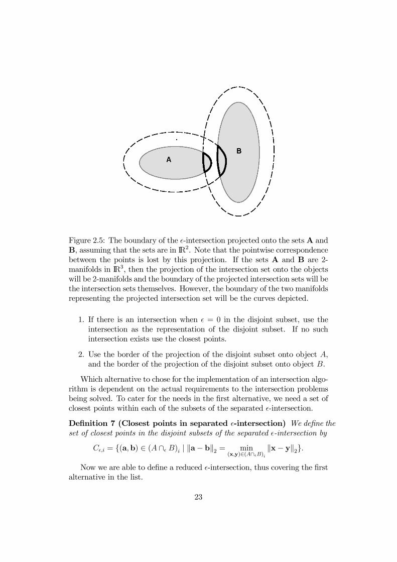
Figure 2.5: The boundary of the -intersection projected onto the sets A andB, assuming that the sets are in IR2. Note that the pointwise correspondencebetween the points is lost by this projection. If the sets A and B are 2-manifolds in IR3, then the projection of the intersection set onto the objectswill be 2-manifolds and the boundary of the projected intersection sets will bethe intersection sets themselves. However, the boundary of the two manifoldsrepresenting the projected intersection set will be the curves depicted.

1. If there is an intersection when = 0 in the disjoint subset, use theintersection as the representation of the disjoint subset. If no suchintersection exists use the closest points.

2. Use the border of the projection of the disjoint subset onto object A,and the border of the projection of the disjoint subset onto object B.

Which alternative to chose for the implementation of an intersection algo-rithm is dependent on the actual requirements to the intersection problemsbeing solved. To cater for the needs in the first alternative, we need a set ofclosest points within each of the subsets of the separated -intersection.

Definition 7 (Closest points in separated -intersection) We define theset of closest points in the disjoint subsets of the separated -intersection by

C ,i = (a,b) ∈ (A ∩ B)i | ka− bk2 = min(x,y)∈(A∩ B)i

kx− yk2.

Now we are able to define a reduced -intersection, thus covering the firstalternative in the list.

23

Definition 8 (Reduced Separated -Intersection) We define the reducedversion of the disjoint subsets of the separated -intersection by

R ,i =

½(A ∩B) ∩ (A ∩ B)i if (A ∩B) ∩ (A ∩ B)i 6= ∅

C ,i if (A ∩B) ∩ (A ∩ B)i = ∅

fori = 1, . . . , N .

As already mentioned, the reduced separated -intersection can have acomplex topological structure, e.g. in surface intersection a number of inter-section curves can meet in a point, or surface regions can meet other regionsor curves in single points.To cover the second item in the list we first make a projection of the

separated -intersection (A ∩ B)i, i = 1, . . . , N onto set A and set B. Thenwe address the boundaries of these projections.

Definition 9 (Projected Separated -Intersection) We define the pro-jection of the disjoint subsets of the separated -intersection by

(A ∩ B)Ai = p ∈ A | (p,q) ∈ (A ∩ B)i , i = 1, . . . , N

(A ∩ B)Bi = q ∈ B | (p,q) ∈ (A ∩ B)i , i = 1, . . . , N .

Remark 2 By the projection we loose the correspondence between the pointsin set A and B taking part in the intersection. The correspondence is in gen-eral not one to one, thus the storage and handling of such a correspondenceis not a trivial task.

Since (A ∩ B)i are closed sets, the projected sets must be closed sets.Thus, the intersection can be represented by the boundary of these sets.

Definition 10 The Boundary of the Projected Separated -Intersection isdefined by

B (A ∩ B)Ai = (A ∩ B)Ai − int((A ∩ B)Ai ), i = 1, . . . , N

B (A ∩ B)Bi = (A ∩ B)Bi − int((A ∩ B)Bi ), i = 1, . . . , N .

Remark 3 Here it is important to distinguish the boundary of the projectedseparated -intersection in IRl from the boundary of the manifolds describ-ing each projected separated -intersection. E.g. a projected separated -intersection in IR3 can consist of a complete circle. The boundary of thecircle in IR3 is the circle itself. However, the circle as a manifold has noboundary since no point on the circle is locally homeomorphic to IR+.

24

2.4 Finding all Intersection Occurrences

In definition 5 we introduced the disjoint separated -intersection. However,we did not discuss any method for singling out the disjoint subsets. The mainstrategy employed to solve such problems is divide and conquer. However, tomake a successful divide and conquer strategy we have to solve the followingproblems:

• Decide if two objects have a guaranteed intersection, a possible inter-section or no intersection. This is addressed in sections 2.4.1 and 2.4.3.

• Decide how to split an -intersection into possible disjoint subsets. Thisis addressed in Section 2.4.2 and Section 2.4.5.

• Identification of a disjoint subset in the separated -intersection. Thisis addressed in Section 2.4.4.

• To decide when a disjoint subset in the separated -intersection consistsof only one bounded manifold, or of touching bounded manifolds ofpossibly different dimensions. This is crucial for the representation ofthe intersection, and is addressed in Section 2.4.6.

• To decide if all disjoint subsets in the separated -intersection set touchthe boundary of one of the objects being intersected. This can reducethe problem to intersecting the boundaries of each of the sets with theother set. This is addressed in Section 2.5.

When we introduced the reduced separated -intersection in definition 8,and the boundary of the disjoint subsets of projected separated -intersectionin definition 10, we did not address the internal topology of these sets. Thiscan in the case of surface intersection consist of one or more points, curvesand surfaces regions. A divide and conquer strategy can be employed whensorting out the topology of each disjoint subset of a projected separated -intersection. The divide and conquer strategy is in general successful sinceit is possible to position a subdivision border between the curves/regions.However, when curves and/or regions meet, the subdivision has to go throughthe points where the curve(s) and/or regions meet. The orientation of thesubdivision border is crucial to the success of the divide and conquer strategy.An other challenge is that between a situations where it is obvious that

the -intersection can be split into disjoint subsets, and situations where the-intersection cannot be split, there are cases where a minor pertubationmakes the subsets touch. Some algorithmic approaches detect in such casesa separation, while other algorithmic approaches detect no separation in

25

the same situations. The reason for such differences can be the nature ofpropagation of rounding errors in different algorithms.The concepts of absolute and relative rounding errors, error propagation,

algorithms minimizing rounding errors and the best representation formatswith respect to rounding error, play a central role to minimize the size ofthe regions where decisions are difficult to make. The divide and conquerstrategy is not efficient in such regions.

2.4.1 Spatial Separation with Respect to a Tolerance

The detection of just one intersection point between two sets establish thefact that the two sets intersect. Thus, strategies than can detect some inter-section point are of great value in the intersection process. By intersectingthe boundary of a compact set A with a compact set B, and the boundary ofB with A, we detect a subset of the intersection. When we later on want torepresent the intersection result, these boundary intersections would be nat-ural to use as candidates in the intersection representation. The boundarypoints are also important since we can use a recursive subdivision strategyto isolate regions where the intersection consists of manifolds that touch theboundary of a closed and bounded smooth manifold, as described in Section2.5.A number of different techniques exists for deciding if two objects are

spatially separated. Two main approaches exist:

• Bounding each of the objects by a simpler geometry and checking ifthese bounding geometries intersect.

• Separating the objects by a geometric object.

In general a coarse bounding geometry is faster to calculate than a finebounding geometry. When comparing two bounding geometries the complex-ity of the bounding objects has significant influence on the performance ofthe test.The most commonly used bounding geometries are:

• Axis-Parallel Boxes. In IR these are intervals; in IR2 axis parallel rec-tangles; in IR3 axis parallel rectangular boxes; and in IRl l-dimensionalaxis parallel boxes.

Axis parallel boxes are easy to calculate for NURBS represented geome-tries with positive weights, as the geometry is limited by the projection

26

of the vertices from the projective space to the affine space. Alge-braically represented geometries are in the general case infinite. How-ever, if they are represented in barycentric coordinates, the corners ofthe barycentric coordinate system describe a triangle in IR2, a tetra-hedral in IR3, and a l-simplex in IRl. By applying the convention thatthe part of algebraic geometry of interest is inside the l-simplex, theproblem is reduced to checking:

— If two simplices are closer than the tolerance .

— If a simplex and a box is closer than the tolerance .

— If two axis parallel boxes are closer than the tolerance .

• Boxes with Fixed Rotation. Naturally the axis parallel boxes arewell behaved for geometries that are axis parallel. However, if the geom-etry is non-axis parallel, then these boxes are a very coarse boundinggeometry. Making boxes from all possible rotations of the coordinatemain axis by 45 degrees is computationally inexpensive, and handlesmany of the non-axis parallel situations well.

• Convex Hulls. An alternative bounding geometry for a NURBS curveor NURBS surface with positive weights is to calculate a convex hullof the control polygon. The calculation requires more operations thancalculating the bounding boxes, and the comparison of two convex hullsis more computational demanding than comparison of boxes.

We can use algebraically represented geometries to separate two manifoldsof possibly different dimensions.

• Separation by Algebraic Hypersurface. Let two manifolds be Aand B, and let an algebraically represented hypersurface be q(x) = 0.If we have that:

∀(pA,pB) ∈ A×B : q(pA) ≥ 0 ∧ q(pB) < 0,

then the objects are non-overlapping. Taking then an overlap within atolerance q > 0 into consideration. We have to satisfy the equation

∀(pA,pB) ∈ A×B : q(pA) ≥ q ∧ q(pB) ≤ − q

to guarantee separation. The value of q has to be calculated from thebehavior of q(x) in the region around setA and setB. The hypersurfacecan be a plane; another hypersurface; a hypersurface containing the

27

manifold A; a hypersurface approximating the manifold A. In Chapter4 we enter into details of such approximative implicitization. In Section4.11 we look at more details on using an algebraic surface for separatingtwo manifolds.

In [Hohmeyer:92] the separation of objects was divided into spatial sepa-rability and spherical separability, the former consisting of bounding boxes,bounding planes, separating planes; the latter including spherical boundingboxes and separating circles. We see that all these concepts are included inthe list above.

2.4.2 Subdividing -Intersections into Disjoint Subsets

Depending on the representation format of the manifolds, more or less nu-meric stable and efficient subdivision algorithms exist. For subdividing ob-jects represented with the Bernstein basis, the de Casteljau algorithm is theobvious choice [Farin:92]. For subdividing B-spline represented objects the“Oslo algorithm” is to be preferred based on the numerical stability of theknot insertion scheme [Fuggeli:93].For algebraically represented geometry, a de Casteljau algorithm can be

used for subdividing, provided that a Bernstein basis in barycentric coordi-nates is used. The part of the algebraic surface of interest is supposed to beinside the simplex defining the barycentric coordinate system.The main challenge in the subdivision process is to decide where to split

the objects. The simplest strategies are:

• For a parametric (tensor product) NURBS represented geometry withinternal knot(line)s, split at an internal knot(line).

• For a parametric rational (tensor product) Bernstein (B-spline with nointernal knot(line)s) represented geometry, split at the midpoint.

• For a barycentric Bernstein basis represented geometry, split at themiddle of the barycentric coordinate system. E.g. for a barycentric co-ordinate system in IRl split at the midpoint: The point with barycentriccoordinates ( 1

l+1, . . . , 1

l+1).

• After reading these thesis Prof. T. W. Sederberg pointed out that a bet-ter strategy for subdividing a barycentric Bernstein basis representedtriangle is to split the triangle into four triangles.

28

These strategies do not take into consideration the actual geometric prob-lem to be solved. By doing this more optimal points for subdivision can befound.The identification of a disjoint subset of a separated -intersection is a

non-trivial task. The set can have a complicated geometric description. Itcan be necessary to break the intersection result into smaller pieces before wecan identify a piece as a piece of a disjoint subset of a separated -intersection.A strategy that can be employed is to subdivide the sets A and B into

subsets having a “monotonous” behavior with respect to each other. Thus,we have to identify how to subdivide the sets to get subsets that are more“monotonous” with respect to each other than the original sets A and B.One approach is to subdivide sets A and B at local minimal points withrespect to the distance function. Another approach is to subdivide the setA in its internal local maximal points with respect to B and the set B in itsinternal local maximal points with respect to A. These issues are addressedin respectively subsections 2.4.3 and 2.4.4 following.

2.4.3 Subdivision at Points with Minimal Distance

By subdividing at local minimum points of the distance function, we can getdifferent effects.

• In theorem 14 and corollary 15 in Section 2.5.2 we develop a result thatidentifies intersection situations, where all objects in the intersectiontouch a boundary of one of the closed and bounded manifolds beingintersected. The theorem allows singular intersection points at theboundaries of the manifolds being intersected. It thus supports subdi-vision in local closest points. Subdivision in these points is, providedthe manifolds being intersected are smooth, a strategy for bringing sin-gular points or near singular points to the boundary of submanifoldsof the manifolds being intersected. By singular points in an intersec-tion we mean points in the intersection with parallel normals. By nearsingular points we mean point pairs in the -intersection with parallelnormals.

• By subdividing at local closest points that are separated more than thegeometric tolerance , we can exclude regions of the manifolds that arefurther apart than .

29

Figure 2.6: Example of local closest points between two curves. Closestpoints where the curves intersect are marked with a gray disk. Noncoinci-dent local closest points are connected by a dashed line. Splitting of thecurves at corresponding closest points can be used to exclude regions formthe -intersection. Splitting at coincident closest points can bring intersec-tion points to the boundary of submanifolds, then those can be analyzed tofind the structure of the intersection set.

The local closest points are defined by the set Smin( ) where the toleranceis a tool for eliminating points lying inside the user defined tolerance.

Smin( ) = (p,q) ∈ A×B | ∃δ > 0 :< kp− qk2 ≤ min

p0∈A∩B(p,δ)∧q0∈B∩B(q,δ)kp0 − q0k2.

The open ball B(p, r) is defined by B(p, r) = y | kp− yk2 < r.

2.4.4 Subdivision at Points with Maximal Distance

The Hausdorff distance d(A,B) between two compact sets A,B ⊂ IRl definesthe global maximal points between the two sets. The distance is in [Degen:92]defined by

d(A,B) := max(maxp∈A

(minq∈B

kp− qk2),maxq∈B(minp∈A

kp− qk2)). (2.1)

We now intend to find points in the two sets that can be called localmaximal points. The set of these points will be denoted Imax(A,B). Lookingat (2.1) we see that the outer maximum is over two expressions where thesets A and B change roles. We take the first of these,

maxp∈A

(minq∈B

kp− qk2), (2.2)

30

and get a simpler expression. However, the roles of A and B are no longersymmetric. We are still finding the “max min” values over the entire sets Aand B. To make the “max min” values local, we can limit the part of A andB used. A way of doing this is to use the following way for defining subsets:

• A subset of A defined by A ∩ B(p, δ) where p ∈ A and δ > 0.

• A subset of B defined by B ∩ B(q, δ) where q ∈ B and δ > 0.

Here B(x, r) is an open ball defined by

B(x, r) = y | kx− yk2 < r .

We require that an element in Imax(A,B) is related to the expression

maxp0∈ A∩B(p,δ)

minq0∈ B∩B(q,δ)

kp0 − q0k2 . (2.3)

Since we use open balls it is easy to find combinations of p, q and δ thatmake (2.3) define no value. However, when (2.3) defines a value we havefound a local maximal point in set A with respect to B. The actual locationis so far not identified. The next step is thus to link the local maximal pointsto p and q. First we link p to the maximum in (2.3) by requiring

minq0∈ B∩B(q,δ)

kp− q0k2 = maxp0∈ A∩B(p,δ)

minq0∈ B∩B(q,δ)

kp0 − q0k2.

When (2.3) defines a value, the expression above must be true for somep ∈ A. Now we link q to the maximum by requiring

kp− qk2 = minq0∈ B∩B(q,δ)

kp− q0k2 = maxp0∈ A∩B(p,δ)

minq0∈ B∩B(q,δ)

kp0 − q0k2.

When (2.3) defines a value, the expression above must be true for someq ∈ B.Thus, we have an expression that describes the properties of what we

want to denote “Local maximal points of a set A with respect to a set B”.

Definition 11 (Local Maximal Points.) Let A and B be two compactsets. The set of Local Maximal Points of A with respect to B is definedby

Imax(A,B) = (p,q) ∈ A×B | ∃δ > 0 : kp− qk2 =min

q0∈ B∩B(q,δ)kp− q0k2 = max

p0∈ A∩B(p,δ)min

q0∈ B∩B(q,δ)kp0 − q0k2.

31

Figure 2.7: The local maximal points Imax(A,B) of set (curve) A with respectto set (curve) B. The arrows point at points of curve B. Note that only oneend point of A is included. Let a point move along curve A from left to right.At the left end, where the point moves away from curve B, the endpointis excluded. Then a point moves along curve A from right to left. At theright end, where the point move closer to curve B, the end point is included.The radius of curvature of curve B is infinite, and is thus greater than thedistance to curve A. Hence for every point on curve A, only one point oncurve B is included.

Figure 2.8: The local maximal points Imax(B,A) of set (curve)B with respectto set (curve) A. The arrows point at points of curve A. Note that bothend points of B are included, one corresponding to an end of A the othercorresponding to an internal point on A. Also note that to some of the pointson B two points correspond on curve A.

32

Remark 4 It is important to note than in general Imax(A,B) 6= Imax(B,A).

Remark 5 If the set B is a smooth manifold, and (p,q) ∈ Imax(A,B), thenthe vector p − q is orthogonal to the tangent bundle of B at the point q,provided q is an internal point in B. This is used in the examples in figure2.7 and in figure 2.8.

Example 12 Let A have the shape of a ∪ and let B be a bar ¯ above the ∪.The intersection problem looks like: ∪ . Now Imax(A,B) contains the bottomof the ∪ paired with the middle point of the bar, while Imax(B,A) containsthe middle point of the bar paired with the end points of ∪.

There are two possible applications for the local maximal points betweenthe two compact sets.

• Let (p,q) ∈ Imax(A,B), and let kp− qk2 ≤ , where ≥ 0 is theintersection tolerance, then we can find an open ball B(p, δ) around pwith radius δ and a ball B(q, δ) around q with radius δ such that

maxp0∈A∩B(p,δ)

minq0∈B∩B(q,δ)

kp0 − q0k2 ≤ ,

i.e. we have detected a part of an -intersection.

• Let (p,q) ∈ Imax(A,B), and let kp− qk2 > , where ≥ 0 is theintersection tolerance, then we can find an open ball B(p, δ) around pwith radius δ and a ball B(q, δ) around q with radius δ such that

maxp0∈A∩B(p,δ)

minq0∈B∩B(q,δ)

kp0 − q0k2 > ,

i.e. we have detected a region that is not part of the -intersection.Subdividing the set A through p and the set B through q may dividethe intersection result into two disjoint sets.

2.4.5 Orientation of the Subdivision Borders

Some of the candidate points for locating the subdivision borders can be onthe boundary of a manifold. When subdividing in those points, we have toselect subdivisions that produce subsets.An aspect to take into consideration when subdividing objects is the ori-

entation of the subdivision borders. Using the standard recursive subdivision

33

techniques the shape of the subdivision borders are hyperplanes in the pa-rameter domain of the parametric geometries, or hyperplanes in IRl for thealgebraically represented geometries. The actual orientation of these hyper-planes, plays a central role in making a successful subdivision. In the tensorproduct parametric case it is efficient, in some cases, to convert to a paramet-ric barycentric representation. In the barycentric representation it is easierto make an optimal orientation of subdivision borders.

2.4.6 Separating Connected Intersection Regions

Now assume that we have a separated -intersection that consists of a setof connected intersection regions that cannot be described by a single mani-fold. We want to describe each intersection region by a bounded manifold ofdimension g , g > 0, each region can have different values for g.Thus, we search for boundary points in respectively (A ∩B)Ai , (A ∩B)Bi

and R ,i, i = 1, . . . , N that are not homeomorphic to IRg+, g ∈ IN. Wesubdivide the problem in such points to make intersection objects that onlycontain manifold geometries.Since we have introduced two reduced representations for the separated

-intersection, we must expect that the intersection geometry and topologyfor the two alternatives in many cases are different.

2.5 Loop Elimination

In the previous section we proposed different strategies for deciding where tosubdivide two objects being intersected to get smaller and possibly simplerintersection problems. We proposed to subdivide in singular or near singularpoints and in points that would give the subsets a more monotonic behaviorwith respect to each other. Now we analyze intersection (sub)problems. Theintention is to find situations when all objects in the intersection result touchthe boundary of one of the objects being intersected. When this is the casewe find points on all intersection objects by just intersecting the boundaryof each set with the other set. It is assumed in the rest of the section thatthe sets intersected are smooth bounded manifolds with a boundary.The smoothness requirement is necessary since the relative orientation of

the geometries is essential to the results presented. The section is structuredas follows:

• The normal set, which is used to describe the orientation of a manifold,is addressed in Subsection 2.5.1.

34

• In Subsection 2.5.2, theorem 14, we establish conditions identifyingwhen n smooth closed and bounded (l−1)-manifolds in IRl intersect inobjects that touch the boundary of one of the (l− 1)-manifolds. Thenwe look at uses of the theorem.

• In Subsection 2.5.3, we show that the boundaries of a manifold haveto be split into pieces, to find the number of intersection objects alongthe boundary.

• Then, in Subsection 2.5.4, we find sufficient conditions for identifyingnonsingular points in the intersection of l smooth (l − 1)-manifolds inIRl.

• The potential of combining algebraically represented hypersurfaces witha manifold is discussed in Subsection 2.5.5.

2.5.1 The Set of Normals

In order to discuss the relative orientation of manifolds, we have to be able todescribe the orientation of each of the manifolds involved in the intersection.For curve segments in IR3 the orientation at a point is related to the curvetangent at that point. The orientation of the curve is described by thepossible tangent directions of the curve segment. The orientation of higherdimensional manifolds is in a similar way described by tangent bundles.Let A be a smooth manifold, then to every point p ∈ A, a tangent bundle

tp, is associated. The tangent bundle is spanned by the first order partialderivatives of the parametrization of A at p. However, we prefer to usenormals of the manifold to describe the orientation and thus introduce theconcept of the Normal Set.

Definition 13 (Normal Set) The set of normals N (A) of A, a smoothmanifold of dimension g in IRl, is defined by

N (A) = q ∈ IRl | kqk2 = 1 ∧ q ⊥ tp, p ∈ A.

where tp is the tangent bundle of A at p.

What is the consequence of this definition? For a bounded l-manifold inIRl, the normal set is empty. For a plane in IR3 the normal set consists ofthe positive and negative unit normal vectors to the plane. For a sphere thenormal set is the entire Gaussian Sphere.

35

2.5.2 Intersections Touching the Boundaries

In [Hohmeyer:92] a theorem was presented for singling out situations wherethe intersection between two surfaces in IR3 has no internal closed curves.The theorem was a significant improvement over the previous work available.In [Hohmeyer:92] an extensive survey of previous work was given including[Dokken:90], [Kriezes:90-1], [Kriezes:90-2], [Kriezes:91], [Mountaudouin:89],[Sederberg:88], [Sederberg:89-1] and [Sinha:85]. Recent work can be foundin [?], [Krishnan:96] and [?]. The following theorem addresses the situationwhen n manifolds in IRl of dimension (l − 1) are intersected. The theoremallows singular intersection points on the boundary of the manifolds beingintersected. In [Hohmeyer:92] all intersection points on the boundaries hadto be nonsingular.

Theorem 14 Let An = Aini=1 be a set of bounded smooth (l−1)-manifoldswith boundary in IRl, l > n > 1. If n1, . . . ,nn are linearly independent, andlinearly independent from a vector v for any ni ∈ N (int(Ai)), i = 1, . . . , n,then

• All r-manifolds r 6= l− n and r < l− 1 in the intersection between themanifolds in An are at the boundaries of one of Ai, i = 1, . . . , n.

• The intersection geometries in the internal of the intersection betweenthe manifolds in An are (l−n)-manifolds that intersect the boundary ofone of Ai, i = 1, . . . , n. I.e. the (l− n)-manifolds do not form internalloops.

If n1, . . . ,nn are linearly independent, and linearly independent from avector v for any ni ∈ N (Ai), i = 1, . . . , n, then all intersections are r-manifolds r ≤ l − n.

Proof. If the smooth (l − 1)-manifolds intersect in a r-manifold, r > l − nand the r-manifold is interior to all the smooth (l−1)-manifolds, then at eachpoint of the intersection the normals of at least two of the l−1manifolds haveto be linearly dependent. This contradicts the assumption that n1, . . . ,nnare linearly independent for any ni ∈ N (int(Ai)), i = 1, . . . , n.Assume that a r-manifold r < l−n is an intersection and is interior to all

the smooth l− 1 manifolds. In a neighborhood of an intersection point p allthe (l− 1)-manifolds Ai, i = 1, . . . , n can be approximated with hyperplanesthrough the point p with normals taken from the respective (l−1) manifolds.These hyperplanes intersect in a (l−n)-manifold since the normals are linearlyindependent. Since all (l − 1)-manifolds are smooth, there is a small region

36

around p where the intersection is a l − n manifold. Thus, the intersectioncannot be an isolated r-manifold, r ≤ l − n− 1.Assume that the intersection consists of a bounded (l − n)-manifold not

touching the boundaries of any Ai, i = 1, . . . , n. The (l − n)-manifold issmooth since all Ai, i = 1, . . . , n are smooth and the normal sets are linearlyindependent. Now choose the direction vector v that is supposed to belinearly dependent from any ni ∈ N (Ai), i = 1, . . . , n. Since the (l − n)-manifold is smooth we can find a hyperplane that is normal to v and tangentto the (l − n) manifold at some tangent point pT .To analyze the tangent bundle at pT , we make a hyperplane hv through

the origin with normal vector v. The tangent(bundle) at pT has to lie in thishyperplane. Looking at which normals of Ai, i = 1, . . . , n that can makea tangent(bundle) in the hyperplane hv, we see that the tangent bundle isspanned by (l − n) linearly independent vectors, the vectors normal to thetangent bundle have to lie in a linear n-manifold. We know that v is onevector in this n-manifold. The linear n-manifold can thus only interpolate(n − 1) of the n-normal vectors, since the n normal vectors are linearlyindependent from v. This implies that the tangent bundle cannot be definedfrom the normal vectors ni ∈ N (Ai), i = 1, . . . , n, and contradicts that pTlies on the (l− n)-manifold in the intersection. Thus, it is impossible for the(l − n)-manifold to not touch the boundary.If the normals set are linearly independent also on the boundaries of

the manifolds, then all intersections of the manifolds are r-manifolds withr ≤ l − n.

Remark 6 Since a g-manifold g ≤ l− 2 can be described as the intersectionof g manifolds of dimension (l − 1), the theorem is also relevant for theintersection of manifolds with lower dimension than l − 1.

Remark 7 The use of theorem 14 for values of n > 2 requires efficientalgorithms for determining the linear independence of (l − n) normal sets,and to decide if there exists a direction v not spanned by the normal sets.

In the case n = 2 the corollary following is dealing with the intersectionof two (l−1)-manifolds in IRl. It states that if the normal sets in the interiorof the manifolds can be separated by two planes, then all intersection curvestouch the boundary of one of the manifolds. A remark then follows concerningthe intersection of two surfaces (2-manifolds) in IR3.

Corollary 15 Let two hyperplanes in IRl through the origin be defined by thenormal vectors b1 and b2. Let A1 and A2 be bounded smooth (l−1)-manifolds

37

with boundary in IRl, l > 2. If the normal sets of int(A1) and int(A2) canbe separated by two hyperplanes i.e.

∀n1 ∈ N (int(A1)) ∧ ∀n2 ∈ N (int(A2)) :(b1 · n1)(b2 · n1) > 0 ∧ (b1 · n2)(b2 · n2) < 0,

then

• All r-manifolds r ≤ l− 3 in the intersection set between A1 and A2 areat the boundary of A1 or A2.

• The intersection geometries in the internal of A1 and A2 are (l − 2)-manifolds that intersect the boundary of A1 or A2. E.g. the (l − 2)-manifolds do not form internal loops.

Proof. Unit vectors lying in the intersection of the two hyperplanes arelinearly independent of the normal sets. Thus, the requirements of theorem14 are satisfied.

Remark 8 The theorem in [Hohmeyer:92] used two planes going through theorigin to separate the normal sets of two surfaces in IR3, and thus to assurethat they are linearly independent, this is corollary 15 for l = 3 and n = 2.Corollary 15 is a more general result than the theorem in [Hohmeyer:92] sincecorollary 15 allows for parallel normal vectors, if they are at the boundary of amanifold. The distinction is important since corollary 15 gives the possibilityfor subdividing manifolds at points where the normals of the manifolds areparallel. Thus, the probability of creating subproblems of the intersection,where all objects in the intersection result touch the boundary, is increased.

The next corollary addresses situations where we can find linear inde-pendence between a vector v and only a subset of the normals sets of the(l − 1)-manifolds being intersected.

Corollary 16 Let An = Aini=1 be a set of closed and bounded smooth (l−1)-manifolds in IRl, l > 2. Let An,r = Ai(j)rj=1 be a subset of An satisfying:n1, . . . ,nr are linearly independent, and linearly independent from a vector vfor ∀nj ∈ N (int(Ai(j))), j = 1, . . . , r, then the internal intersections lie on(l − r)-manifolds that touch the boundaries, and result from the intersectionof the manifolds in An,r.Proof. The intersection of the manifolds in An is a subset of the intersectionof the manifolds of An,r. For An,r theorem 14 can be applied.

38

Remark 9 The corollary can be used for identifying the possible location ofintersection objects, when the linear independence of the normal vectors andthe direction v is not established for the complete intersection problem, butcan be established for a subset of the set of manifolds. Thus, regions whereno intersection objects exist can be excluded by analyzing the intersection ofthese subsets.

Example 17 Let p(s, t), (s, t) ∈ Ω be a smooth surface with positive weightsin IR3, where Ω is a rectangle in IR2, and let a straight line be described bythe intersection of the two planes q1(x) = 0 and q2(x) = 0. Define three2-manifolds in IR3 by

A1 = (s, t, q1(p(s, t))), (s, t) ∈ ΩA2 = (s, t, q2(p(s, t))), (s, t) ∈ ΩA3 = (s, t, 0), (s, t) ∈ Ω.

(2.4)

The intersection of the three manifolds A1, A2 and A3 is equivalent to theintersection of the surface and the straight line. In theorem 23 in Subsection2.5.4 conditions for when an intersection results in nonsingular points aregiven. If a possible singular situation arise, corollary 16 can be used forlooking at the three intersection problems A1 ∩ A2, A1 ∩ A3 and A2 ∩ A3 toestablish the possible location of the intersection result.

In the following example we create an intersection between a straight lineand a ruled surface resulting in a singular situation.

Example 18 Let the surface p(s, t) be a ruled surface in IR3 defined by thetwo curves p(s, 0) and p(s, 1) i.e.

p(s, t) = (1− t)p(s, 0) + tp(s, 1), (s, t) ∈ [smin, smax]× [0, 1].

Let p(c, t), c ∈ [smin, smax] denote a straight line. Let q1(x) = 0 and q2(x) = 0be the algebraic description of two noncoincident planes intersecting alongp(c, t). The intersection problem can be formulated as (2.4) and is singular.Provided the two curves p(s, 0) and p(s, 1) do not intersect, the intersec-tion curve p(c, t), c ∈ [smin, smax] is nonsingular in at least two of the threeintersection problems A1 ∩A2, A1 ∩A3 and A2 ∩A3.

In the following corollary we apply theorem 14 to a smooth function ing-variables, defined over a compact domain Ω, to establish conditions whenthe zeroes of the function lie on a (g− 1)-manifold that touch the boundaryof Ω.

39

Corollary 19 Let Ω ∈ IRg, g > 1 denote a compact set, and let f denote aC1 continuous function f : Ω→ IR satisfying for some d ∈ IRg

d · ( ∂f∂s1

, . . . ,∂f

∂sg) > 0, (s1, . . . , sg) ∈ int(Ω). (2.5)

Then the set of zeroes of f

IΩ = (s1, . . . , sg) ∈ Ω | f(s1, . . . , sg) = 0

satisfies

• All manifolds of dimension p < g − 1 in IΩ are at the boundary of Ω.

• The manifolds in IΩ in the internal of Ω have dimension (g − 1), andintersect the boundary of Ω. I.e. the (g − 1)-manifolds do not forminternal loops.

Proof. We convert the problem to a (g+1) dimensional problem by definingtwo g-manifolds for (s1, . . . , sg) ∈ Ω

f0(s1, . . . , sg) = (s1, . . . , sg, 0)

f1(s1, . . . , sg) = (s1, . . . , sg, f(s1, . . . , sg)).

The internal normal set of f0 and f1 are:

N (int(f0)) = (0, 1)

N (int(f1)) = (∇f(s1, . . . , sl), 1) | (s1, . . . , sl) ∈ int(Ω).

By assumption (2.5), vectors from the two normal sets, are linearly indepen-dent. Further vectors in the intersection of:

• The hyperplane normal to (d, 0) through the origin,

• The hyperplane normal to (0, . . . , 0, 1) through the origin,

cannot be made by a linear combination of the two normal sets. Thus, avector v exists linearly independent from N (int(f0)) and N (int(f1)) and theconditions of theorem 14 are met.Now the question is the practical construction of the vector d in the

corollary above.

40

Example 20 Assume that the function f is described as a NURBS function.∂f(s,t)∂s

and ∂f(s,t)∂t

are then NURBS functions. Thus, (∂f(s,t)∂s

, ∂f(s,t)∂t) is a convex

combinations (provide positive weights) of a set of 2D vectors. Adding these,or their normalized version, gives a dominant direction of (∂f(s,t)

∂s, ∂f(s,t)

∂t). In

case the sum is zero, the vectors cannot be located at one side of a line throughthe origin, and the separation is impossible. Given the dominant directionwe can calculate a “direction” cone of (∂f(s,t)

∂s, ∂f(s,t)

∂t). If the opening of the

direction cone is less than π, we have obtained the required separation.

Example 21 Let p(s, t), (s, t) ∈ Ω denote a NURBS surface with positiveweights in IR3, that is to be intersected with an algebraic surface q(x) = 0. Thefunction q(p(s, t)) is of the type described in corollary 19. Corollary 19 canthus be used for identifying situations where all intersections of p(s, t), andthe algebraic surface q(x) = 0, in the internal of Ω, are curves (1-manifolds)that touch the boundary of Ω.

In appendix B other problems where corollary 19 can be used are dis-cussed.

2.5.3 Boundary Subdivision Necessary

In theorem 14 conditions were established for identifying situations whenintersection results touch the boundary of one of the closed and boundedsmooth manifold intersected. Thus, in such situations, we can look at thebehavior of the boundary of a manifold, to describe the intersection results.

Theorem 22 Let A be a closed and bounded smooth manifold with a smoothboundary denoted B. Then the Normal Set from (see definition 13) of theboundary B denoted, N (B) spans the entire Gaussian sphere.

Proof. Assume that there is a direction v /∈ N (B), i.e. v is not in thenormal set of the boundary B. Make a hyperplane with normal vector vthat do not touch B. By translation of the hyperplane we can bring itto a position where the hyperplane just touch the boundary B. Since B issmooth the hyperplane is tangential to B and v must be in the N (B). Thus,contradicting that v /∈ N (B).

Remark 10 Often the boundary of a closed and bounded smooth manifoldis not smooth. By smoothing out regions on the boundary, where the tangentbundle has breaks, we get a manifold with a smooth boundary, and theorem22 can be used. Thus, it is natural to define the normal set of the boundary

41

of a closed and bounded smooth manifold as the entire Gaussian Sphere. Theconsequence is that the normal set contains no information on the orientationof the boundary. For use in intersection algorithms, the boundary has to besplit into pieces, for the normal set to be of practical use.

A tensor product surface has a rectangular parameter domain. Thus, afirst choice is to split the boundary into the four curves corresponding to thestraight lines defining the rectangular parameter domain. Triangular surfaceshave a triangular parameter domain. The primary choice is thus to subdivideinto three boundary curves, each corresponding to one of the straight linesdescribing the triangular parameter domain.

2.5.4 Finding Nonsingular Intersection Points

Figure 2.9 illustrates a helix that, when intersected with certain axis parallelstraight lines, gives a number of intersection points. This happens althoughthe normal vectors of the helix, and the tangent direction of the straightline are never orthogonal. Since the straight line can be described as theintersection of two planar surfaces, the intersection can also be viewed as theintersection of 3 surfaces in IR3. In this section we look at the intersection ofl smooth manifolds of dimension (l − 1) in IRl.

Theorem 23 Give A = Aili=1 a set of closed and bounded smooth (l− 1)-manifolds, with boundaries, in IRl, l > 1. Let n1, . . . ,nn be linearly inde-pendent for any ni ∈ N (int(Ai)), i = 1, . . . , n. Let for i = 1, . . . , l , Di beA with manifold Ai removed. Then

• All objects in the intersection between the manifolds in A, not lying onthe boundary of any of the manifolds in A, are nonsingular points.

• The intersection points lie on 1-manifolds touching the boundary of oneof the manifolds in Di, for i = 1, . . . , l.

Proof. For an internal intersection point to be singular, at least two man-ifolds must have the same tangent plane. Since the normal sets are linearlyindependent, this is impossible.By removing one manifold theorem 14 is applicable, and the internal

intersections are 1-manifolds touching the boundary.Now going back to figure 2.9, we see that the normal sets of the planar

surfaces intersecting in the straight line and the helix are linearly indepen-dent. Thus, all the intersection points are nonsingular, and we can generatecurves on which the intersection points lie.

42

Figure 2.9: The intersection of a helix and a straight line parallel to the helixaxis can produce a number of intersection points although the tangent of thestraight line and the possible normals of the helix are never orthogonal.

43

2.5.5 Combining Parametric and Algebraic Represen-tations

A common technique in intersection algorithms is to combine algebraic andparametric descriptions as described in Chapter 4. For certain geometricobjects, e.g. the second degree algebraic curves and surfaces, we know bothdescriptions.Let h(s) be a parametric represented manifold of dimension g in IRl,

g < l, and let fi(ti), i = 1, . . . , n be manifolds in IRl that lie respectively inthe hypersurfaces fi(x) = 0, i = 1,. . . , n. Then instead of intersecting themanifolds h(s) and fi(ti), i = 1, . . . , n, we can look at the problem

f1(h(s)) = . . . =fn(h(s)) =0. (2.6)

This problem can further be reformulated to the intersection of (n+1) man-ifolds of dimension g in IRg+1. These manifolds are

g0(s) = (s, 0)gi(s) = (s, fi(h(s)), i = 1, . . . , n.

(2.7)

Since fi(fi) ≡ 0, i = 1, . . . , n, the solution of (2.7) contains the solutions ofthe original intersection problem in IRl. The dimension of the reformulatedproblem (2.7) is smaller than that of the original intersection problem.If we can find a sufficiently good approximation fi(x) = 0 to fi(x) = 0

close to fi for i = 1, . . . , n, then we have a method for finding approximativesolutions to the original intersection problem. In Chapter 4 we look at suchapproximative implicitization.

44

Chapter 3

Representation of GeometricObjects

3.1 Parametric Representation of Closed andBounded Manifolds.

Parametric representation of manifolds in IR2 and IR3 by piecewise polyno-mials is much used in CAGD-systems. It is well known that Bernstein andB-spline basis functions have a better numerical behavior, when used for suchrepresentation, than the power basis, see e.g. [Farouki:87]. In the approxi-mative implicitization method presented in Section 4.3, stable and accurateproducts of powers of the coordinate functions of the manifolds are central.The approximative implicitization method is not limited to manifolds in IR2

and IR3, but addresses manifolds of dimension g in IRl with 1 ≤ g < l. Theproperties needed in the basis functions, used for the parametric descriptionof the manifolds to be approximated, are assembled in definition 24. Thisdefinition includes the following basis functions:

• Tensor product Bernstein basis.

• Bernstein basis defined over a simplex.

• Tensor product B-spline basis.

• Possibly certain subclasses of linear independent Box-spline and sim-plex splines bases. However, we do not address these possibilities in thisthesis. For more information on multivariate splines see e.g. [Seidel:92].

When making products of the coordinate functions of a parametric rep-resented manifold, we can without much loss of generality assume that the

45

coordinate functions are represented with the same basis functions. For ourpurpose it is convenient to let the description of any of these bases consistof:

• A Description of the Polynomial Degree or Degrees of the basisfunctions, in the following described by the multi index n or m.

• A Geometric Description of the Piecewise Polynomial Struc-ture, i.e. of how the domain of the basis functions is split into piecewisepolynomial segments. We denote this description by the multi index t.

• A Description of the Continuity between adjacent piecewise poly-nomial segments. This is denoted by the multi index c.

We refer to this as the PosProd basis description. The PosProd basisfunctions are denoted

Bi,n(s) = Bci,n,t(s),

here i ∈ In = Ici,n,t is a set of multi indices for the basis functions. s is avector with a dimension corresponding to the dimension of the parameterdomain. We denote the number of multi indices Nn. The following definitiononly use the formBi,n(s), because t and c are constants for the multiplicationoperations of interest.

Definition 24 (PosProd Basis Function) Let Scn,t be a space of piece-wise polynomials of degree n and continuity c with a geometric description tdefined over the compact domain Ω. In addition let Scn,t contain the poly-nomials of degree n. A basis Bi,ni∈In for Scn,t is called a PosProd basisif

1. It is a partition of unity and the basis functions are nonnegativeXi∈In

Bi,n(s) = 1, s ∈ Ω

withBi,n(s) ≥ 0, s ∈ Ω, i ∈ In.

2. The product h(s) ∈ Scm+n,t of the two functions p(s) ∈ Scn,t and q(s) ∈Scm,t with nonnegative coefficients has nonnegative coefficients. If

p(s) =Pi∈In

piBi,n(s), pi ≥ 0, i ∈ Inq(s) =

Pi∈Im

qiBi,m(s), qi ≥ 0, i ∈ Im.

46

Thenh(s) = p(s)q(s) =

Xi∈Im+n

hiBi,m+n(s)

withh(s) ∈ Scm+n,t,

andhi ≥ 0, i ∈ Im+n.

The name PosProd reflects that the product of two PosProd representedfunctions p and q with nonnegative cofficients results in a PosProd repre-sented function h with with nonnegative cofficients.

Definition 25 (PosProd Algorithm) Given the product of two positivefunctions, which both are represented by PosProd Basis functions. APosProdAlgorithm ensures that the relative rounding errors in the coefficients of theproduct are limited by the relative rounding errors of the functions multiplied.If p (s) and q (s) are respectively p(s) and q(s) from condition 2 in definition24 with imposed relative rounding errors

p (s) =Xi∈In

pi(1 +pi )Bi,n(s), pi ≥ 0, i ∈ In

q (s) =Xi∈Im

qi(1 +qi )Bi,m(s), qi ≥ 0, i ∈ Im,

where| pi | ≤ p

max ∧ (pi = 0 =⇒ pi = 0), i ∈ In

| qi | ≤ q

max ∧ (qi = 0 =⇒ qi = 0), i ∈ Im.

Then the product of p (s) and q (s) must satisfy

h (s) = p (s)q (s) =X

i∈Im+n

hi(1 +hi )Bi,n+m(s)

with ¯hi

¯≤ p

max +qmax +

pmax

qmax, i ∈ Im+n.

Remark 11 It should be observed that the description of the PosProd basisfunctions representing the product of two PosProd represented functions areconstructed by keeping the geometry description t and the continuity descrip-tion c fixed, and just adding the polynomial degrees m and n.

Example 26 (Univariate B-spline) Let the PosProd description of the B-spline basis be:

47

• Description of polynomial degree n.

• Description of piecewise polynomial structure by strictly increasing knotvalues

t = tiηi=1 .

• Description of continuity at each knot value

c = ciηi=1 = −1, c2, . . . , cη−1,−1

with 0 ≤ ci ≤ n− 1, i = 2, . . . , η − 1.

Here η is the number of distinct knot values. The number of basis func-tions in a B-spline basis is (see Theorem IX.1 page 113 in [de Boor:78]) :

“Polynomial order”+“Number of internal knots” = n+ 1 +

η−1Xi=2

(n− ci).

Products of m functions represented in this B-spline basis have the samedistinct knot values and continuity. However, the polynomial degree is raisedto mn. Thus, the number of basis functions of degree mn is

Nmn = mn+1+

η−1Xi=2

(mn− ci) = (η− 1)mn−Ã

η−1Xi=2

ci

!+1 ≤ (η− 1)mn+1.

In the case of a piecewise Bernstein basis representation the number of basisfunctions of degree mn is

Nmn = (η − 1)(mn+ 1).

The amount of basis functions save by using a B-spline representationinstead of a Bernstein representation is

Nmn − Nmn = (η − 1) +Ã

η−1Xi=2

ci

!− 1 = η +

Ãη−1Xi=2

ci

!− 2.

This number is independent of the number m of functions in the product .Thus, if a piecewise Bernstein basis representation is used instead of a B-spline representation the relative overhead with respect to the number of basisfunctions decrease as m increase.

48

Example 27 (Univariate B-spline) Let the knot vector defining a B-splinebasis be

t = 1, 1, 1, 1, 2, 2, 2, 3, 3, 4, 5, 5, 5, 5 .The PosProd basis description is

n = 3t = 1, 2, 3, 4, 5c = −1, 0, 1, 2,−1 .

The product of two such 3rd degree bases yields the PosProd basis description

n = 6t = 1, 2, 3, 4, 5c = −1, 0, 1, 2,−1 .

The product of the 3rd degree basis and 6th degree basis gives the PosProdbasis description

n = 9t = 1, 2, 3, 4, 5c = −1, 0, 1, 2,−1 .

Example 28 (Bi-variate B-spline basis.) The polynomial degree is n =(k1 − 1, k2 − 1), where k1 and k2 are the polynomial orders in the two pa-rameter directions of the tensor product B-spline basis. The description ofthe piecewise polynomial structure t is two lists of knot values, one for eachparameter direction. The continuity c is two lists of numbers, one list foreach knot value list. The lists give as, in the univariate case, the continuityat each knot value.

Next we deal with a theorem showing that product algorithms based onconvex combinations are PosProd Algorithms. Then two corollaries relatingthe result to the Bernstein basis and to the B-spline basis follow.

Theorem 29 Let p(s) and q(s) be two functions represented with PosProdbasis functions of respectively degree m and n with the same piecewise poly-nomial structure t and the same continuity description c. Further let theproduct algorithm used for generating the coefficients hr ∈ Im+n of h(s) =p(s)q(s) be based on sums of convex combinations of products of the coeffi-cients of p(s) and q(s):

hr =Xi∈In

Xj∈Im

γri,jpiqj, r ∈ Im+n,

49

where Xi∈In

Xj∈Im

γri,j = 1, r ∈ Im+n

withγri,j ≥ 0, r ∈ Im+n, i ∈ In, j ∈ Im.

Then the product algorithm is a PosProd Algorithm.

Proof. Let as in definition 25 p (s) and q (s) be respectively p(s) andq(s) with imposed rounding errors. Then the coefficients hr , r ∈ Im+n ofh (s) = p (s)q (s) satisfy

hr =Xi∈In

Xj∈Im

γri,jpi (1 +pi ) qj

¡1 + q

j

¢=

Xi∈In

Xj∈Im

γri,jpiqj +Xi∈In

Xj∈Im

γri,jpiqj(pi +

qj +

pi

qj )

= hr(1 +hr),

where

hr =

⎧⎪⎨⎪⎩i∈In j∈Im

γri,jpiqj(pi+

qj+

piqj )

i∈In j∈Imγri,jpiqj

if ∃γri,jpiqj 6= 0

0 if ∀γri,jpiqj = 0.If there exist γri,jpiqj 6= 0 we have, since γri,j, pi and qj all are nonnegative,that h

r is a convex combination of (pi +

qj +

pi

qj ), i ∈ In, j ∈ Im thus¯

hr

¯≤ max

i∈In,j∈Im

¯pi +

qj +

pi

qj

¯≤ p

max +qmax +

pmax

qmax,

which is the requirement in definition 25 of a product algorithm to be aPosProd Algorithm. If all γri,jpiqj = 0 then

¯hr

¯= 0, which also satisfies

definition 25.

Corollary 30 In [de Boor:87-1] and [Farin:86] multiplication formulas aregiven for multiplication of functions represented in the tensor product Bern-stein basis and for multiplication of functions represented in a Bernstein basisover a simplex. These multiplication formulas are based on sums of convexcombinations of products of the coefficients of the functions being multiplied,and are thus by theorem 29 PosProd Algorithms.

Error analysis of the B-spline basis is more difficult than the error analysisof the Bernstein bases. In [Cox:72] the first backwards error analysis on theB-spline recursion formulas was given. Here we show that there exist PosProdAlgorithms for tensor product B-splines.

50

Corollary 31 In [Moerken:91-1] a product algorithm for univariate B-splinerepresented functions is given. This product algorithm is based on sums ofconvex combinations of products of the coefficients of the functions beingmultiplied. The multiplication algorithm is thus by theorem 29 a PosProdAlgorithm.For functions represented in a tensor product B-spline basis, the products

can be performed one variable at a time. Thus, performing multiplication onevariable at the time using the algorithm in [Moerken:91-1] for tensor productB-splines, gives us a PosProd Algorithm.

Remark 12 The method for the multiplication of B-spline represented func-tions is so resource demanding, that a good alternative is to use a knot inser-tion algorithm to represent the function on a Bernstein knot vector. I.e. aknot vector where all knots have multiplicity corresponding to the polynomialorder. Then the method for the multiplication of tensor product Bernsteinbasis represented functions can be used on each polynomial segment in thetensor product B-spline basis.

The concept of PosProd Basis Functions can possibly also be applicablefor certain subclasses of Box-splines and for simplex splines. However, forthe PosProd basis concept to be of practical use, there have to be PosProdAlgorithms for these types of multivariate splines. As far as the author ofthe thesis knows, no such algorithms have been developed.More details on PosProd bases are given in Appendix A. We also consider

rational functions and manifolds defined from PosProd basis functions.

Definition 32 (R-Positive Manifold) Let l and g be integers with g < l.Given a compact set Ω ⊂ IRg and a PosProd basis Bi,n(s), i ∈ In definedover Ω. A function p : Ω → IRl which for some real numbers c1i , . . . , c

li and

chi can be written in the form

p(s) =Xi∈In

(c1i , . . . , cli)

chiαi,n(s), s ∈Ω (3.1)

with

αi,n(s) =chiBi,n(s)X

j∈In

chjBj,n(s), i ∈ In,

andchj > 0, j ∈ In,

is called a R-positive manifold in IRl of degree n. The numbers chj , j ∈ Inare called the weights of the R-positive manifold.

51

Remark 13 The set of R-positive manifolds includes:

• Rational tensor product Bernstein represented manifolds with positiveweights.

• Manifolds represented by a Rational Bernstein basis with positive weightsdefined over a simplex.

• Tensor product NURBS represented with positive weights.

The nonrational versions of these are included in the definition, becausesetting chj = 1, j ∈ In, makes the denominator equal to 1 and the manifoldsnonrational.

3.2 The Algebraic Hypersurface

Suppose that q ∈ Pm(IRl), i.e. that q is a polynomial of total degree m in l

variables. Then ©x ∈ IRl | q(x) = 0

ª(3.2)

is called an algebraic hypersurface.Traditionally the polynomial q defining the algebraic hypersurfaces is rep-

resented in the power basis

q(x) =X

i1+...+il+1=m

ij≥0, j=1,...,l+1

ai1,...,il

lYj=1

xijj .

However, describing the algebraic hypersurface using a simplex S in IRl

and representing the polynomial in a Bernstein basis in barycentric coordi-nates defined over S, has desirable numerical properties in the algebraic im-plicitization process to be described. The ealiest us of this approach knownto the author of this thesis can be found in [Sederberg:84-2]. The Bernsteinbasis in barycentric coordinates over a simplex S is described in appendixA.2. In this representation we have

q(x) =Xi∈I(m)

bim!

i!βi(x) (3.3)

with

i! = i1! . . . il+1!

βi(x) =l+1Yj=1

¡βj(x)

¢ij ,52

and

I(m) = (i1, . . . , il,il+1) ∈ INl+10 | 0 ≤ ij ≤ m−

j−1Xp=1

ip, j = 1, . . . , l + 1.

Here β1(x), . . . , βl+1(x) are barycentric coordinates with respect to S, andthus they satisfy

l+1Xi=1

βi(x) = 1

withβi(x) ≥ 0, x ∈ S.

53

Chapter 4

Approximative Implicitization

In Sections 2.4.1 and 2.5.5 the advantage of combining algebraic and paramet-ric representations of the manifolds to be intersected was discussed. However,for most parametric surfaces it is difficult to find the algebraic representationas discussed in Chapter 12 in [Hoschek:93]. The conclusions in this referenceare:

• To find the exact algebraic representation of a 2D polynomial para-metric curve can be done by building the Bezout resultant. The per-formance and accuracy of such an implicitization is good enough tobe used in CAGD applications. The polynomial degree of the alge-braic representation of a parametric polynomial curve is the same asthe polynomial degree of the parametric representation.

• For parametric surfaces the situation is more complex. A triangularparametric surface of total degree n has an implicit formula of degreen2. A parametric tensor product surface of degree (m,n) has an im-plicit formula of degree 2mn. A bicubic surface patch thus results inan algebraic representation of degree 18 with 1330 terms. Thus, thecomputational complexity of finding algebraic representations for poly-nomial surfaces is high. In [Hoschek:93] references to more details onthis topic are [Chionh:92] and [Sederberg:84-1].

In [Sederberg:95] the practical problems of exact implicitization of curvesand surfaces are addressed. The main problem is that huge expressions areinvolved when performing exact implicitization of surfaces. Another problemis that in the case of base points, points where both numerator and denom-inator of a parametric curve or surface vanish simultaneously, the earlierstandard methods fail. The method described in [Sederberg:95] is a major

54

step in the direction of more applicable exact implicitization methods. In-stead of base points being a problem, these methods use the existence of basepoints to reduce the degree of the algebraic curve or surface found. For asurvey of earlier methods [Hoffmann:93] can be consulted. Details on one ofthese methods, Groebner Bases, can be found in the book [?]. Details onresultant based methods can be found in the book [Cox:98]. In certain casesdirect implicitization methods exist, see e.g. [Floater:95-2] where rationalcubic implicitization is addressed.The problem of finding the algebraic representation of a R-positive man-

ifold of dimension (l − 1) in IRl can be formulated as follows.

Definition 33 (Exact Implicitization) Let l > 1 and p(s), s ∈ IR(l−1) bea R-positive (l−1)-manifold in IRl described as in definition 32. The processof exact implicitization of p(s) is to find a nontrivial polynomial q ∈ Pm(IR

l)of minimal degree m such that

q(p(s)) = 0, s ∈ IR(l−1).

We restrict the definition to R-positive manifolds to avoid introducingadditional concepts. All geometry representations that can be converted toa R-positive manifold of dimension (l− 1) are thus covered. In remark 13 inSection 3.1 we dealt with manifolds represented with a rational tensor prod-uct Bernstein basis or a rational Bernstein basis over a simplex. We statedthat those have a R-positive description provided the weights are positive.Power basis represented manifolds can be converted to these descriptions andare thus covered provided the resulting weights are positive.Exact implicitization is as stated in [Sederberg:95] and [Hoschek:93] a

difficult problem. In addition if an exact implicit representation is found, thepractical use of the implicit representation can be difficult, because:

• The polynomial degree is often high.

• Singular points near or on the implicit representation can give undesiredproperties if finite precision arithmetic is used.

Since CAGD systems are based on floating point representation, all repre-sented geometries are affected by a small relative rounding error. Thus, whenwe find the “exact” algebraic representation, it is influenced by a roundingerror.

Example 34 Let a straight line segment be represented as a Bezier curveof degree 3. If the representation is exact, then the algebraic degree of the

55

straight line is 1. Represented in a float format on a computer small roundingerrors are assigned to the vertices representing the straight line. Thus, the“straight line” probably has algebraic degree 3 when converted to infinite pre-cision. Using methods that find the exact algebraic representation can thusresult in an algebraic representation with a higher polynomial degree thannecessary.

In this chapter we address approximative implicitization of R-positivemanifolds in IRl. We allow for the approximation of a manifold of dimensiong by hypersurfaces in IRl also for g < l−1. Thus, we are able to approximatea manifold of dimension g by the intersection of l − g hypersurfaces.

Definition 35 (Approximative Implicitization) Let l and g be integerswith 1 ≤ g < l, and let p(s), s ∈ Ω ⊂ IRg be a R-positive manifold ofdimension g in IRl. The nontrivial algebraic hypersurface q(x) = 0, q ∈Pm(IR

l), is an approximative implicitization of p(s) within the tolerance ≥ 0if we can find a continuous direction function g(s) and a continuous errorfunction η(s) such that

q(p(s) + η(s)g(s)) = 0, s ∈ Ω,

wherekg(s)k2 = 1, s ∈ Ω,

and|η(s)| ≤ , s ∈ Ω.

g(s) is called the direction for error measurement.

Sometimes it is convenient, to simplify the use of the algebraic approx-imation q(x) = 0, to require that the gradient of q(x) is nonvanishing in asufficiently large region around p(s), s ∈ Ω. This additional condition is,however, not part of the definition. If the gradient of q(x) vanish on p(s) ortoo close to p(s), estimates for the error function η(s), cannot be based onthe gradient of q(x).An alternative to the approximative implicitization method described in

this chapter, is as studied in [Sederberg:90], by minor modifications to insertbase points in the parametric description of p(s). Thus, the degree of thealgebraic description is reduced and the algorithms in [Sederberg:95] thattake benefit from the existence of base points, can be used.We focus in this chapter on building the theoretical foundation for an

algorithm for approximative implicitization of p(s). The structure of thechapter is as follows:

56

• In Section 4.1 we show that the composition of an algebraic hyper-surface q(x) = 0, with q(x) described as in (3.3) and a R-positiveg-manifold p(s), described as in definition 32, can be expressed

q(p(s)) = (Db)Tα(s),

where D is a matrix, b contains the coefficients of q and α(s) containsthe basis functions used for representing products of the coordinatefunctions of p. This means that if b is in the null space of D, thenq(p(s)) = 0. Moreover

|q(p(s))| ≤ kDbk2 .

The matrix D has desirable numeric properties if the coefficients ofp(s) are contained in a simplex S, and this simplex is used for thedescription of q in barycentric coordinates.

• In Section 4.2 we show that the relative rounding errors of the entriesin D are well behaved, when PosProd Algorithms are used for buildingthe matrix.

• In Section 4.3 we show that

minkbk2=1

maxs∈Ω

| q(p(s)) | ≤ σ1.

Where σ1 ≥ 0 is the smallest singular value of D when barycentriccoordinates are used for describing the algebraic hypersurface, and p(s)is contained in the simplex defining the barycentric coordinate system.This result shows that singular value decomposition can be used forfinding an algebraic approximation of a R-positive manifold.

• In Section 4.4 we show how constraints can be added to the algebraicapproximation to control the behavior of the approximation. Then inSubsection 4.4.5 we show that rows in the matrix D can be used asconstraints in a direct elimination process as an alternative to singularvalue decomposition.

• In Section 4.5 we establish the convergence rate of the algebraic approx-imation and show that this is high especially for the approximation ofparametric curves by algebraic curves (approximation of 1-manifolds inIR2).

• In Section 4.6 we look at how to measure the error of an algebraicapproximation to a manifold.

57

• In Section 4.7 we introduce the concept of admissable algebraic approx-imation, as an attempt to establish a tool for evaluating the quality ofan algebraic approximation.

• In Section 4.8 we look at a method for choosing an approximation, witha possibly well behaved gradient, from the approximative nullspace ofD.

• In Section 4.9 we give a more detailed version of the following algorithm:

Algorithm Approximative Implicitization

1. Choose the algebraic degree m of q.

2. Choose the barycentric coordinate system to be used in the ap-proximation such that p(Ω) is inside the simplex defining thebarycentric coordinate system.

3. Build the matrixD of coefficients combining the characteristics ofq and p.

4. Find an approximative null space of D.

5. Choose as coefficients of q a vector from the approximative nullspace with a “good” gradient behavior.

6. Check if the hypersurface is admissible. If not admissable increasethe number of vectors in the approximative null-space and go to4.

7. Check if the hypersurface is within the prescribed tolerance . Ifnot within the tolerance, try with a higher algebraic degree orperform the approximation on a smaller part of p.

• In Section 4.10 we look at how a number of manifolds of possibly dif-ferent dimensions can be approximated by one algebraic hypersurface.

• In Section 4.11 we describe how to find a hypersurface intended forspatially separating two manifolds. Then we look at how to estimatethe distance between the manifolds by using such a hypersurface.

• The chapter is concluded in Section 4.12 by examples of approximativeimplicitization of a degree 7 parametric Bezier curve.

In sections 4.1 through 4.5 the results presented are based on the man-ifolds being R-positive. However, we only refer to these as manifolds org-manifolds inside these sections to simplify the presentation.

58

4.1 Combining Parametric Manifolds and Al-gebraic Hypersurfaces

In this section we look at the properties of the matrix D mentioned in theintroduction. It is assumed that the algebraic hypersurface is of total degreem and represented in barycentric coordinates. The combination q(p(s)) is afunction of degree mn in the variable(s) s.The combination q(p(s)) can be used:

1. To build the matrix/vector structure used in the approximative implic-itization process.

2. For transforming an intersection problem to a zero value problem asdescribed in Section 2.5.5.

The results in this section and in the section following are useful to keepthe relative rounding errors in q(p(s)) at a minimal level.The first step is theorem 36 reformulating q(p(s)) to an expression using

rational basis functions. Based on this, corollary 37 reformulates the sum toan expression of vectors and matrices

q(p(s)) = (Db)T α(s).

The theorem then following limits |q(p(s))| by kDbk2, thus getting rid ofα(s). The remainder of the section is devoted to analyze the numericalproperties of the matrix D.Important steps in this section are:

• The isolation of the coefficients of the algebraic hypersurface in onevector b.

b =³bj´Mj=1

.

The entries in the vector b are related to the coefficients, bj, j ∈I(m),of the algebraic hypersurface q(x) = 0 by a lexicographical ordering ν

bν(j) = bj, j ∈I(m).

We also use the inverse ν−1 of the lexicographical ordering giving

bν−1(j) = bj, j = 1, . . . , M .

59

• The isolation of the variables used for the parametrization of the man-ifold in a vector α(s), also denoted the α-basis.

α(s) = (αi(s))Nmn

i=1 .

The entries in the vectorα(s) are related to the rational basis functions,αi,mn(s), i ∈Imn, of a manifold by a lexicographical ordering γ

αγ(i)(s) = αi,mn(s), i ∈Imn.

We also use the inverse γ−1 of the lexicographical ordering γ giving

αi(s) = αγ−1(i),mn(s), i = 1, . . . , Nmn.

• The isolation of expressions dependent of the coefficients of the mani-fold in a matrix D. The entries in D are functions of the coefficientsof the coordinate functions of p(s).

D =³di,j´Nmn,M

i,j=1,1. (4.1)

We also use the lexicographical ordering ν and γ and their inverse forthe ordering of the entries of the D matrix.

In the proof a transformation from the Bernstein basis to the α-basisplays a central role. Thus, the first step is to represent q(p(s)) in this basis.

Theorem 36 Let p(s) be a R-positive manifold defined as in definition 32,and let q(x) = 0 be a hypersurface described in barycentric coordinates as in(3.3). Then

q(p(s)) =Xi∈Imn

⎛⎝ Xj∈I(m)

djibj

⎞⎠αi,mn(s), (4.2)

where dji satisfy

m!

j!βj(p(s)) =

Xi∈Imn

djiαi,mn(s), j ∈ I(m).

Proof. We have from (3.3) that

q(p(s)) =Xj∈I(m)

bjm!

j!βj(p(s)).

60

Remembering that βj(p(s)) is a product of m of the coordinate functions ofp(s), we have that the polynomial degree of βj(p(s)) ismn. Thus, m!

j!βj(p(s))

can be expressed in the α-basis of degree mn. We denote these coefficientsdji and get

m!

j!βj(p(s)) =

Xi∈Imn

djiαi,mn(s), j ∈ I(m)

givingq(p(s)) =

Xj∈I(m)

bjXi∈Imn

djiαi,mn(s).

Now rearranging the sum we get (4.2).We are, at this stage, not addressing how this basis conversion is achieved

only that it is possible. We show in Section 4.2 that using PosProd Algo-rithms for this transformation, limits the growth of relative rounding errors.

Corollary 37 Let l and g be integers with 1 ≤ g < l. Given q(x) = 0, an al-gebraic hypersurface in IRl of degree m represented in barycentric coordinatesas defined in (3.3), and p(s) ∈ IRl, a g dimensional manifold as defined indefinition 32. Then

q(p(s)) = (Db)T α(s). (4.3)

Proof. From theorem 36 we have

q(p(s)) =Xi∈Imn

⎛⎝ Xj∈I(m)

djibj

⎞⎠αi,mn(s)

=NmnXi=1

⎛⎝ MXj=1

dν−1(j)γ−1(i)bν−1(j)

⎞⎠αγ−1(i),mn(s) (4.4)

=NmnXi=1

(MXj=1

di,j bj)αi(s)

= (Db)T α(s),

where

di,j = dν−1(j)γ−1(i)

bj = bν−1(j)

αi(s) = αγ−1(i),mn(s).

61

In the following theorem we utilize the fact that PosProd basis functionsare the partition of unity, to remove the vectorα(s) containing the variable(s)s used in the parametrization of the manifold.

Theorem 38 Let the algebraic hypersurface and the manifold be as in corol-lary 37 and definition 32. Let s ∈ Ω, e.g. be in the support of the basis of themanifold. Then

|q(p(s))| ≤ kDbk2 . (4.5)

Proof. For any s ∈ Ω we have by definitionNmnPi=1

αi(s) = 1 and 0 ≤ αi(s) ≤ 1,

i = 1, . . . , Nmn. Thus, kα(s)k2 ≤ 1, giving

|q(p(s))| =¯(Db)Tα(s)

¯≤ kDbk2 kα(s)k2 ≤ kDbk2 .

In the following theorem we show that if the algebraic hypersurface isdefined by a barycentric Bernstein basis over a simplex, and that the simplexcontains the manifold, then the matrix D has desirable numeric properties:

• All entries are none negative.

• The sum of all entries in a row is one.

• The Frobenius norm of D is limited by the number of rows.

Theorem 39 Let D be defined as in (4.1). Then

MXj=1

di,j = 1, i = 1, . . . , Nmn. (4.6)

If the coefficients of the manifold is contained in the simplex defining thebarycentric coordinate system in which q(x) is described, then

di,j ≥ 0, i = 1, . . . , Nmn, j = 1, . . . , M , (4.7)

and

kDk2F =NmnXi=1

MXj=1

³di,j´2=

MXj=1

σ2j ≤ Nmn. (4.8)

Here k kF is the Frobenius norm, and σi, i = 1, . . . , M are the singularvalues of D.

62

Proof. Choose b = (1, . . . , 1)T , then q(x) = 1 giving

q(x) =NmnXi=1

⎛⎝ MXj=1

di,j

⎞⎠αi(s) = 1.

SinceNmnXi=1

αi(s) = 1,

and αi(s) are linearly independent, we have

MXj=1

di,j = 1 .

Thus, (4.6) is proved.Since the coefficients of the manifold are contained in the simplex defin-

ing the barycentric coordinate system, the coefficients of the barycentric rep-resentation of the manifold are all nonnegative. In addition, because themanifold is R-positive the weights of the manifold are by definition positive.Thus, all the elements in D are greater than or equal to zero, as all func-tions involved in the multiplication process making D have none negativecoefficients, and we use a PosProd basis. Thus, proving (4.7).Because 0 ≤ di,j ≤ 1, we have that 0 ≤ (di,j)2 ≤ di,j ≤ 1, resulting in

kDk2F =NmnXi=1

MXj=1

³di,j´2≤

NmnXi=1

MXj=1

di,j =NmnXi=1

1 = Nmn

proving (4.8). The connection between the Frobenius norm and the sum ofthe squares of the singular values can be found in standard books on linearalgebra e.g. in [Stewart:73].In CAGD applications we are most often interested in 1-manifolds in IR2,

1-manifolds in IR3 or 2-manifolds in IR3. The results in theorem 39 are in-dependent of the dimension of the space in which the manifold lies. In theexample following we assume that the conditions of theorem 39 are satis-fied, and look at the size of Nmn for 1-manifolds represented by nonuniformrational B-splines (NURBS).

Example 40 Let the PosProd description of the B-spline basis used fordefining the 1-manifold be as in example 26 on page 47. Then

kDk2F ≤ (η − 1)mn+ 1,

63

where η is the number of distinct knot values, m is the algebraic degree and nthe polynomial degree of the B-spline basis. In the case of a Bernstein basisη = 2 and

kDk2F ≤ mn+ 1.

4.2 Stable Building of the D Matrix

When the matrix D, defined in (4.1), is constructed from a R-positive g-manifold p(s), the entries result from products of powers of the coefficientsof the coordinate functions of p(s). The number of coordinate functionsinvolved in such a product is the total degreem of the algebraic hypersurfaceq(x) = 0. In this section we limit the relative rounding error of these products

(p(s))j =l+1Yi=1

(pi(s))ji ,

where j = (j1, . . . , jl+1) satisfying

l+1Xi=1

ji = m ≥ 1,

andji ≥ 0, i = 1, . . . , l + 1.

We require that PosProd Algorithms are used when building the D matrix.

Theorem 41 Let pi : Ω→ IR, i = 1, . . . , g be functions represented with thesame PosProd basis functions with nonnegative coefficients. Let p ,i(s) i =1, . . . , g be respectively pi(s), i = 1, . . . , g with imposed relative roundingerrors, and let the relative rounding errors of the coefficients satisfy

| pii |≤ max, i ∈ In, i = 1, . . . , g.

Given ji ∈ IN0, i = 1, . . . , l + 1 that satisfy

m =l+1Xi=1

ji. (4.9)

Then provided a PosProd Algorithm is used for evaluating the coefficientshji, i ∈ Imn of

(p(s))j =Xi∈Imn

hjiαi,mn(s)

64

the relative rounding errors(pj)i , i ∈ Imn of the coefficients hji, i ∈ Imn

satisfy ¯(pj)i

¯≤

mXi=1

µm

i

¶imax. (4.10)

Proof. For m = 1, only one of ji, i = 1, . . . , l + 1 are different from zero.Assume that this is jt. By (4.9) jt = 1. Now

(pj)

i reduce to¯(pj)i

¯= | pti | ≤ max,

which is (4.10) for m = 1.Assume (4.10) is true for m = k =

Pl+1i=1 ji. Now multiplying by pt,

1 ≤ t ≤ l + 1, using the properties of a PosProd Algorithms on page 47 weget ¯

pt(pj)i

¯≤ pt

max +(pj)max +

ptmax

(pj)max

≤ max +kXi=1

µk

i

¶imax + max

kXi=1

µk

i

¶imax

≤kXi=1

µk

i

¶imax +

k+1Xi=1

µk

i− 1

¶imax

≤kXi=1

µµk

i

¶+

µk

i− 1

¶¶imax +

k+1max

≤k+1Xi=1

µk + 1

i

¶imax.

Which is (4.10) for m = k + 1.

Remark 14 Let the coefficients of a R-positive manifold p(s) ∈ IRl be con-tained in a simplex S used for the definition of a hypersurface in barycentriccoordinates. Since the weights of a R-positive manifold are required to be pos-itive the barycentric representation of p(s) has only non-negative coordinatefunctions. Thus, theorem 41 can be used for limiting the growth of the round-ing errors of D. The consequence of the theorem is that the relative roundingerror is growing with a rate related to the algebraic degree m, since we canexpect that m max ¿ 1, and thus m max is the dominant term in the sumPm

i=1

¡mi

¢i. This reasonably stable combination of algebraic and parametric

surfaces can be achieved by:

65

Algebraic degreem

Relativerounding error Comment

2 2.0× 10−15 Conic sections

3 3.0× 10−15 Algebraic degree ofcubic parametric curve

18 1.8× 10−14 Algebraic degree ofbicubic parametric surface

100 1.0× 10−13m m× 10−15

Table 4.1: Relative rounding errors for different algebraic degrees of the Dmatrix when the R-positive manifold p(s) is defined in a barycentric coordi-nate system containing the coefficients of p(s). The coefficients of p(s) areassumed to have relative rounding errors limited by 10−15.

• Finding a simplex S containing the coefficients of a manifold.

• Represent the manifold in the barycentric coordinates defined by S.

• Represent the algebraic hypersurface by Bernstein basis functions de-fined over S.

Example 42 Assume that we have represented the R-positive manifold inbarycentric coordinates such that the coefficients are inside a simplex S. Us-ing double precision the value 10−15 is typically of the relative rounding errors.Now building the matrix D for different algebraic degrees, we get table 4.1 asa limit for the relative rounding errors of the elements in D.

4.3 Implicitization by Singular Values

How can the results from Section 4.1 be used when approximating a manifoldin IRl? In (4.5) we established a relationship

|q(p(s))| ≤ kDbk2 .

We now relate this expression to the singular values of D.

Theorem 43 Let as in (4.3) p(s) be a R-positive manifold in IRl. Let q(x) =0, be an algebraic hypersurface in IRl with coefficient vector b. Then

minkbk2=1

maxs∈Ω

| q(p(s)) | ≤ σ1. (4.11)

66

Where σ1 ≥ 0 is the smallest singular value of D, where D is defined in(4.1).

Proof. From (4.5) we have |q(p(s))| ≤ kDbk2 when s ∈ Ω. Thus, we canreformulate to

maxs∈Ω

|q(p(s))|2 ≤ bTDTDb.

Now restricting the coefficient vector to have length 1, e.g. kbk2 = 1, andtaking the minimum we get

minkbk2=1

maxs∈Ω

| q(p(s)) |2≤ minkbk2 6=0

bTDTDb

bTb= λmin. (4.12)

Where λmin ≥ 0 is the smallest eigenvalue of DTD. The last equal sign isbased on the fact that DTD is a Hermitian matrix (symmetric matrix) andthat for a Hermitian matrix A the Raleigh quotient x

TAxxTx

satisfies

λmin ≤xTAx

xTx≤ λmax,

where λmin is the smallest and λmax the largest eigenvalue of A. The smallestsingular value of D is σ1 =

√λmin, giving (4.11).

Remark 15 It is important to observe the number of singular values in Dthat are identical zero. If the number exceeds 1, then it is possible that wehave used a higher algebraic degree than necessary in the approximation. Thisalso is an indication that the parametric description of the manifold containsbase points.

In the general case when p(s) ∈ IRl is a R-positive manifold, it is impos-sible to get an exact algebraic representation as a single algebraic equation.This because the R-positive manifold, if it consists of more than one poly-nomial segment, in most cases has some discontinuity of some derivative atsome point. In this case we see from (4.11) that the eigenvector correspond-ing to the smallest eigenvalue, is a solution of a least squares approximationof an algebraic hypersurface to p(s) . Although we find a least squares ap-proximation, there is no guarantee that we find the best solution. E.g. thechoice of barycentric coordinate system influences D. In addition the be-havior of the gradient of the algebraic hypersurface determines how accuratethe approximation is. How to find an approximation with a well behavedgradient is addressed in Section 4.8.

67

4.4 Constraining the Algebraic Equation

To better integrate approximations of R-positive g-manifolds into geometricmodeling systems, we introduce in this section different ways to constrainthe algebraic approximation to adhere to different sorts of constraints. Weuse manifolds of dimension l to define the constraints. The dimension ofthe manifolds being applied as interpolation constraints, is in most cases lessthan the dimension of the manifold being approximated. The constraintsare:

• Interpolation of a manifold is addressed in subsection 4.4.1. Often itis desirable that the approximation interpolates given points. For 1-manifolds (curves) the points are often the start and end points, for 2-manifolds (surface) the points are often break points on the boundary ofthe 2-manifold. For 2-manifolds the constraining manifolds can also be1-manifolds (curves). Typical curves applied are the boundary curvesof the 2-manifold. However, curves internal to the manifold or outsidethe 2-manifold can also be used. Internal curves can be used to ensureexact fit to the boundary of another 2-manifold, while external curvescan be used to control the shape of the algebraic approximation outsidethe manifold being approximated.

• Forcing the gradient of the polynomial q(x) used for describing thehypersurface to be orthonogal to a tangent direction varying along amanifold is addressed in subsection 4.4.2. In combination with an in-terpolation constraint this can be used to induce interpolation of amanifold and tangent direction varying along the manifold at the sametime. If the tangent constraint is not accompanied by a position con-straint, then we model the behavior of the gradient of q(x) in a regiondefined by a manifold. If the manifold being approximated is a 1-manifold the typical constraints are tangent at start and end points. Ifthe manifold being approximated is a 2-manifold, then the constraintsare typically the two tangent directions at break points in the boundaryof the 2-manifold or the tangent behavior along the boundary of the2-manifold.

• Forcing the gradient of q(x) to take on a specific behavior along amanifold is addressed in subsection 4.4.3. This can be used to inducesingular regions in the approximation, either inside or outside the man-ifold approximated.

In subsection 4.4.4 we consider how the constraints can be organized in alinear equation system, which can be applied for modifying the matrix vec-

68

tor expression kDbk2 describing the unconstrained approximation problem.Choosing a selection of rows from theD matrix as constraints is addressed insubsection 4.4.5. These can either be the most dominant rows, or rows thatinduce interpolation of position, tangent or higher order derivatives alongthe boundary of the manifold. This approach can also be used for a directsearch for an approximative null space of D.

4.4.1 Interpolation of Position along a Manifold

To impose interpolation of the position over a constraining manifold r(t), wecan use the expressions from equation (4.3) giving

q(r(t)) = (Dkb)T αr(t) = 0.

Remembering that the basis functions in αr(t) are linearly independent wecan reformulate the expression, giving

Dkb = 0. (4.13)

4.4.2 Interpolation of Tangent along a Manifold

The normal of the algebraic hypersurfaces is, provided the gradient is nonva-nishing, parallel with the gradient of the hypersurface. Thus, to ensure thatthe normal is orthogonal to a given direction dr(t) along the manifold r(t)we establish

∇q(r(t)) · dr(t) = 0.Provided both r(t) and dr(t) can be expressed with the same PosProd basisfunctions, we rearrange this expression on the form

∇q(r(t)) · dr(t) =³D

0kb´T

αr(t) = 0.

Further remembering that the basis functions in αr(t) are linearly indepen-dent, we get the constraints

D0kb = 0. (4.14)

4.4.3 Interpolation of Normal along a Manifold

Another possibility is to impose that the gradient takes on certain behaviornr(t) along a given manifold r(t)

∇q(r(t)) = nr(t) =

⎛⎜⎝ n1(t)...

nl(t)

⎞⎟⎠ ,

69

or specifying each coordinate function separately

∂q(r(t))

∂xi= ni(t), i = 1, . . . , l.

Provided r(t) and nr(t) can be express by the same PosProd basis functions,we get

∂q(r(t))

∂xi= (Dn,ib)

T αr(t) = ni · αr(t), i = 1, . . . , l.

Further remembering that the basis functions in αr(t) are linearly indepen-dent, we get the constraints

(Dn,ib)T = ni, i = 1, . . . , l. (4.15)

4.4.4 The Constraint Equation

Combining (4.13), (4.14), (4.15) and possibly rows from the matrixD we caninfluence the result of the algebraic approximation process. The constraintscan be organized as r linearly independent constraints on the algebraic hy-persurface in a set of linear constraint equations:

Kb = h. (4.16)

In the following theorem we assume that the matrix K and b can be split intwo parts

K = (K1,K2) (4.17)

b =

µb1b2

¶. (4.18)

where

• K1 is a nonsingular r × r matrix.

• K2 is a r × (M − r) matrix.

• b1 is a vector of length r.

• b2 is a vector of length (M − r).

We thus assume that the constraints are linearly independent and thatthe number of constraints r is less than the number of coefficients in thealgebraic hypersurface.

70

Theorem 44 Let the combination of a hypersurface and a manifold satisfythe constraint equation defined in (4.16) which is organized as in (4.17) and(4.18) then

|q(p(s))| ≤ kDK0b2 + h0k2 ,

where

K0 =

µ−K−11 K2

I

¶,

and

h0 = D

µK−11 h0

¶.

Proof. Using (4.17) and (4.18), we get

(K1,K2)

µb1b2

¶= h,

givingb1 = K

−11 h−K−11 K2b2.

Resulting in

b=

µ−K−11 K2

I

¶b2 +

µK−11 h0

¶.

Substituting this into (4.5) in lemma 38, we get

|q(p(s))| ≤ kDbk2 (4.19)

≤°°°°Dµ −K−11 K2

I

¶b2+D

µK−11 h0

¶°°°°2

= kDK0b2 + h0k2 .

Remark 16 By pivoting and removing redundant constraints, we can bringany constraint equation to the structure described in (4.17).

Remark 17 When we want to find an algebraic hypersurface approximatinga manifold, a first choice of an algorithm is singular value decomposition ofDK0. This can be used in the case of both when h0 = 0 and h0 6= 0.• For h0 = 0 the problem reduce to |q(p(s))| ≤ kDK0b2k2. Thus, thecoefficient vectors corresponding to the smallest singular values of DK0

are solutions to the approximation problem.

• For h0 6= 0, using e.g. theorem 6.8 in [Stewart:73] the singular valuedecomposition of DK0b2 can be used for finding the vector b2, givingthe minimum of kDK0b2 + h

0k2.

71

4.4.5 Direct Search for an Approximative Null Space

We use rows in the D matrix as constraints, described as in Section 4.4.4,and here assume that the matrix D can be given the structure

D =

µD1,1 D1,2

D2,1 D2,2

¶, (4.20)

where

• D1,1 is a r × r nonsingular matrix.

• D2,1 is a (N − r)× r.

• D1,2 is a r × (M − r) matrix.

• D2,2 is a (N − r)× (M − r) matrix.

Further let b be split as in (4.18)

b =

µb1b2

¶,

where

• b1 is a vector of length r.

• b2 is a vector of length (M − r).

Lemma 45 Let D be built up by the submatrices as described in (4.20) andlet the constraints be described by

D1,1b1 +D1,2b2 = 0. (4.21)

Then

Db =

µ0

−D2,1D−11,1D1,2 +D2,2

¶b2. (4.22)

Proof. Using the constraints we get b1 = −D−11,1D1,2b2, giving

Db =

µD1,1 D1,2

D2,1 D2,2

¶µb1b2

¶

=

µD1,1 D1,2

D2,1 D2,2

¶µ−D−11,1D1,2

I

¶b2

=

µ0

−D2,1D−11,1D1,2 +D2,2

¶b2.

72

In an elimination process it is convenient to maintain the size of thematrices during the process. Thus, we combine the constraint equation intothe result of lemma 45 to maintain the size of D in the lemma following.

Theorem 46 Let D be split as in (4.20) and use (4.21) as constraints. Then

Db =

µI D−11,1D1,2

0 −D2,1D−11,1D1,2 +D2,2

¶µb1b2

¶(4.23)

withµI D−11,1D1,2

0 −D2,1D−11,1D1,2 +D2,2

¶=

µD−11,1 0−D2,1D

−11,1 I

¶µD1,1 D1,2

D2,1 D2,2

¶.

(4.24)

Proof. Rewriting the constraint equation

D1,1b1 +D1,2b2 = 0

we get µI D−11,1D1,2

0 0

¶b = 0.

From (4.22) we have that

Db =

µ0

−D2,1D−11,1D1,2 +D2,2

¶b2 =

µ0 00 −D2,1D

−11,1D1,2 +D2,2

¶b.

Adding the latter equations, we obtain

Db =

µI D−11,1D1,2

0 −D2,1D−11,1D1,2 +D2,2

¶b.

The matrix used for premultiplication in (4.24) can be shown to be correctby multiplying the two matrices.If the entries in the block D2,1D

−11,1D1,2+D2,2 in (4.22) have a sufficiently

small value, then the results in lemma 45 can be used as an eliminationprocess to find an approximative null space ofD. In the theorem following weintroduce conditions that have to be satisfied to control such an eliminationprocess.

Theorem 47 Let D be built by submatrices as described in (4.20), let

D1,1b1 +D1,2b2 = 0,

73

and °°−D2,1D−11,1D1,2 +D2,2

°°∞ ≤ .

Then

minkbk2=1

maxs∈Ω

|q(p(s))| ≤q(N − r)(M − r).

Proof. Using lemma 45 we get

kDbk2 ≤°°−D2,1D

−11,1D1,2 +D2,2

°°∞ kbk2 ≤

q(N − r)(M − r) kbk2 .

Now using (4.12) we get

minkbk2=1

maxs∈Ω

| q(p(s)) |2≤ minkbk2 6=0

bTDTDb

bTb≤ 2(N − r)(M − r)

proving the theorem.The following elimination method is inspired by Gaussian elimination

with pivotation. It starts with the line containing the element with thelargest absolute values as constraint equation and perform the elimination.The elimination is repeated until all lines except one has been used for elim-ination, or the absolute value of the largest remaining element is less than aspecified tolerance. The elimination sequence is remembered as well as thevalue of the largest element at each step in the process. Since the elimina-tion sequence is determined during the elimination process, pointer arraysare used to introduce pivotation. The algorithms is based on theorem 46with added pivotation, and repeated use with the submatrix D1,1 havingdimension 1× 1. The stop condition is based on theorem 47.

Algorithm

1. D = D.

2. Mark all rows and columns in D as untreated.

3. While the maximal untreated element in D is greater than inabsolute value and more than one column untreated:

(a) Let di,j be the untrated element with maximal absolute value.(b) Divide row di by di,j.(c) Eliminate the entries with index j from all other rows of D,

i.e. dl := dl − dl,jdi, l 6= i.

74

(d) Mark row i and column j as treated and remember that coef-ficient j was eliminated in row i, remember the absolute valueof the largest element before the elimination step, as well asthe number of the elimination step.

4. Now all untreated elements have absolute value less than or equalto , or only one column remains.

Remark 18 At the end of this process the matrix has the structure that is arow and column pivotation ofµ

I D−11,1D1,2

0 −D2,1D−11,1D1,2 +D2,2

¶.

If°°−D2,1D

−11,1D1,2 +D2,2

°°∞ ≤ then independent of choice of b2 the

value ofminkbk2=1

maxs∈Ω

| q(p(s)) |2≤ 2(N − r)(M − r),

because kb2k2 ≤ kbk2. Thus, we have found an approximative null space.Since ¡

I D−11,1D1,2

¢µ b1b2

¶= 0,

we can find b1 byb1 = −D−11,1D1,2b2

and thus b by

b =

µb1b2

¶=

µ−D−11,1D1,2

I

¶b2.

The algorithm just described remembers −D−11,1D1,2, thus the approxima-tive null space can be calculated from the reduced approximative null space.

This elimination algorithm performs more slowly than simple implemen-tations of Singular Value Decomposition (SVD). However, it is faster thanSVD implementations requiring DTD to be calculated. The remark, in theoriginal version of these thesis, that the direct search for the approximativenull space was slower than the use of SVD was based on the use of a fast SVD-algorithm that do not always converge. For more information on SingularValue Decomposition the book [Golub & Loan:83] can be consulted.The tried SVD algorithms sometimes fail when the algebraic degree m

is higher than 10 and the calculation is performed in double precision. Inthese cases the smallest singular values of D are separated less than therounding errors in the D matrix. Thus, a minor change in D can induce a

75

major change in the singular subspace of D as stated in theorem 8.3-6. in[Golub & Loan:83]. The SVD implementations report lack of convergence.The reason for the failure is probably that there is an iteration process inthe SVD implementation to speed up the calculation, and this fails when theseparation of the singular values is small compared to the rounding errors.

4.5 Convergence Rate of Approximative Im-plicitization

For approximative implicitization to be useful we need to establish resultson how the approximation error behaves, as the part of the manifold beingapproximated is reduced. The convergence rates established are best for lowdimensional manifolds.

• Approximation of 1-manifolds in IR2 with convergence rate

O(h(m+1)(m+2)

2−1).

• Approximation of 1-manifolds in IR3 with convergence rate

O(h(m+1)(m+2)(m+3)

2−1).

• Approximation of 2-manifolds in IR3 with convergence rate

O(h16

√(9+12m3+72m2+132m)− 1

2 ).

In this section we at first present a theorem on the convergence rate of theapproximation of a hypersurface of degree m to a manifold of dimension g inIRl. Then we analyze the above-referenced convergence rates. However, theconvergence rate can be misleading if the gradient of the hypersurface found,is vanishing or near vanishing, close to the manifold being approximated.The proof of the theorem is based on power expansion around a point

v ∈ Ω, where Ω is the parameter domain of the manifold p approximated.The value of h is used to define a closed hyperbox in Ω around v in thefollowing way:

Ω(v, h) = Ω ∩ s ∈IRg | kv− sk∞ ≤ h .

It should be noted that the matrix D from (4.3) now is dependent on thevalue of v and h.

76

Theorem 48 Given q(x) = 0, an algebraic hypersurface in IRl of degree mwith coefficient vector b, and p(s), a Cn+1-continuous manifold of dimensiong in IRl. Then for v ∈ Ω and h > 0

minkbk2=1

maxs∈Ω(v,h)

|q(p(s)| ≤ minkbk2=1

kDbk2 ≤ O(hn+1),

where n satisfies µn+ g + 1

g

¶≥µm+ l

l

¶>

µn+ g

g

¶.

Proof. Use the description of the algebraic hypersurface in (3.3)

q(x) =Xi∈I(m)

bim!

i!βi(x),

and let

ri(s) =m!

i!βi(p(s)).

Then (4.4) can be written

q(p(s)) =Xi∈I(m)

bi ri(s).

Now assume that s ∈ Ω(v, h), then with s = v + δ, we have that kδk∞ ≤ h.Taylor expansion of ri(s) around v with a polynomial of total degree n gives

ri(v+ δ) = ti(δ) + ei(δ),

where ti(δ) has total degree n, and ei(δ) = O¡(kδk∞)

n+1¢ ≤ O(hn+1). Thenumber of terms in a polynomial of total degree n in g variables isµ

n+ g

g

¶.

The number of coefficients in the algebraic hypersurface isµm+ l

l

¶.

Provided the number of coefficients in the algebraic hypersurface is greaterthan number of coefficients in the polynomial of total degree n, then thepolynomials ti(δ) are linearly dependent. I.e. ifµ

m+ l

l

¶>

µn+ g

g

¶77

we can find coefficients b0 with kb0k2 = 1, such thatXi∈I(m)

b0i ti(δ) = 0. (4.25)

We are interested in the largest natural number n with this property, thuswe state µ

n+ 1 + g

g

¶≥µm+ l

l

¶>

µn+ g

g

¶.

Using the above Taylor expansion, the associated error functions, and thatδ = s− v, we get

q(p(s)) = (Tb)Tα(s) + (Eb)Tα(s)

where(Tb)Tα(s) =

Xi∈I(m)

bi ti(s− v)

and(Eb)Tα(s) =

Xi∈I(m)

bi ei(s− v).

Now remember that ei(s− v) = ei(δ) = O(hn+1), we have that

(Eb)Tα(s) = O(hn+1).

All entries in α(s) are linearly independent, thus all entries in Eb0 must beO(hn+1), giving kEb0k2 = O(hn+1).Now remembering (4.25) and that Tb0 = 0, we get

minkbk2=1

maxs∈Ω(v,h)

|q(p(s))| ≤ minkbk2=1

kDbk2 ≤kDb0k2kb0k2

=k(T+E)b0k2

kb0k2=kEb0k2kb0k2

= O(hn+1).

We now look at curves in IR2 to illustrate the properties of approximativeimplicitization.

Corollary 49 Let q(x) = 0 be an algebraic curve of degree m with coefficientvector b, and let p(s) be a sufficiently smooth 1-manifold in IR2. Then

minkbk2=1

maxs∈Ω(v,h)

|q(p(s)| ≤ minkbk2=1

kDbk2 ≤ O(h(m+1)(m+2)

2−1).

78

Algebraic degree m 1 2 3 4 5 6 7 8 9 10Convergence rate 2 5 9 14 20 27 35 44 54 65

Table 4.2: Convergence rate of the approximative implicitization of a suffi-ciently smooth parametric curve in IR2 with an algebraic curve of degree m,1 ≤ m ≤ 10.

Proof. Let l = 2 and g = 1 in theorem 48 givingµn+ 2

1

¶≥µm+ 2

2

¶>

µn+ 1

1

¶.

Rewriting we get

n+ 2 ≥ (m+ 1)(m+ 2)

2> n+ 1,

or

n =(m+ 1)(m+ 2)

2− 2.

We add 1 to get the convergence rate.

Example 50 In table 4.2 we show the convergence rate from corollary 49.The convergence rate is given for algebraic degrees in the range, 1 ≤ m ≤ 10.Note that the convergence rate is high even for low algebraic degrees.

The corollary following shows that the convergence rate increases as thedimension l of the space in which the 1-manifold lies grow.

Corollary 51 Let q(x) = 0 be an algebraic surface of degree m with co-efficient vector b, and let p(s) be a sufficiently smooth 1-manifold in IR3.Then

minkbk2=1

maxs∈Ω(v,h)

|q(p(s)| ≤ minkbk2=1

kDbk2 ≤ O(h(m+1)(m+2)(m+3)

6−1).

Proof. Let l = 3 and g = 1 in theorem 48 givingµn+ 2

1

¶≥µm+ 3

3

¶>

µn+ 1

1

¶.

Rewriting we get

n+ 2 ≥ (m+ 1)(m+ 2)(m+ 3)

6> n+ 1,

or

n =(m+ 1)(m+ 2)(m+ 3)

2− 2.

We add 1 to get the convergence rate.

79

Algebraic degree m 1 2 3 4 5 6 7 8 9 10Convergence rate 3 9 19 34 55 83 119 164 219 285

Table 4.3: Convergence rate of the approximative implicitization of a suffi-ciently smooth parametric curve in IR3 with an algebraic surface of degreem, 1 ≤ m ≤ 10.

Example 52 In table 4.3 we show the convergence rate from corollary 51.The convergence rate is given for algebraic degrees m in the range, 1 ≤ m ≤10. Note that the extremely high convergence rate is due to the high numberof coefficients in an algebraic surface.

The corollary following show that the convergence rate is lower for 2-manifolds in IR3, than for 1-manifolds in IR2.

Corollary 53 Let q(x) = 0 be an algebraic surface of degree m with coef-ficient vector b, and let p(s, t) be a sufficiently smooth 2-manifold in IR3.Then

minkbk2=1

max(s,t)∈Ω(v,h)

|q(p(s, t))| ≤ minkbk2=1

kDbk2 ≤ O(h16

√(9+12m3+72m2+132m)− 1

2 ).

Proof. Let l = 3 and g = 2 in theorem 48 givingµn+ 3

2

¶≥µm+ 3

3

¶>

µn+ 2

2

¶.

Now finding n such that µm+ 3

3

¶− 1 =

µn+ 2

2

¶,

and using the largest natural number less than the calculated n we get

n(m) =

¹1

6

p(9 + 12m3 + 72m2 + 132m)− 3

2

º.

We add 1 to get the convergence rate.

Example 54 In table 4.4 we show the convergence rate from corollary 53.The convergence rate is given for algebraic degrees m in the range, 1 ≤ m ≤10. Note that the convergence rate is relatively high even for low algebraicdegrees.

80

Algebraic degree m 1 2 3 4 5 6 7 8 9 10Convergence rate 2 3 5 7 10 12 14 17 20 23

Table 4.4: Convergence rate of the approximative implicitization of a suffi-ciently smooth parametric surface in IR3 with an algebraic surface of degreem, 1 ≤ m ≤ 10.

4.6 Accuracy of Approximative Implicitiza-tion

In many cases we want an approximation to be within a certain tolerance> 0 of the object approximated. When we measure the distance from a

manifold p(s) to a manifold q(t) a natural choice for distance measure is

d(p,q) = maxsinftkp(s)− q(t)k2 .

In this definition inf is used since the manifolds are not required to be closed.The distance measure can be interpreted:

• For all points on p find the closest point on q.

• Use the maximum distance found as distance measure.

Note that this expression is similar to (2.2), that we used in the discussionconcluding with the definition of Local Maximal Points of one set with respectto another set.To use the distance function d(p,q) we require a parametric description of

both manifolds. In the case we shall discuss, this is not the case. We have analgebraic hypersurface q(x) = 0 and a parametric represented manifold p(s).To measure the error we now introduce a direction for error measurementg(s) satisfying kg(s)k2 = 1. To be a useful direction for error measurementwe assume that there exists an error function ρ(s) ∈ C0 such that

q(p(s)− ρ(s)g(s)) = 0.

Not all choices for direction for error measurement will satisfy this require-ment. To simplify the notion we now let p = p(s), g = g(s) and ρ = ρ(s).The above equation can then be expressed

q(p− ρg) = 0.

Taylor expansion with respect to ρ now gives

q(p)−∇q(p− θg) · ρg = 0

81

with θρ ≥ 0 and |θ| ≤ |ρ|. Rearranging we getρ (∇q(p− θg) · g) = q(p).

Now settingρmax = max

s∈Ω|ρ(s)| ,

and assuming that

∇q(p− θg) · g 6= 0, s ∈ Ω, |θ| ≤ ρmax

we get, by reintroducing p(s), g(s) and ρ(s)

ρ(s) =q(p(s))

∇q(p(s)− θg(s)) · g(s) (4.26)

with |θ| ≤ |ρ(s)|.We see that the relative orientation of the direction for error measure-

ment, and the gradient of q plays a central role in estimating the error.Thus, an optimal solution is to find a direction for error measurement thatgives the maximum value of the denominator in the expression above. Thisrequirement can be formulated as finding g(s) with kg(s)k2 = 1 that satisfies

mins ∈ Ω,

|θ| ≤ ρmax

|∇q(p(s)− θg(s)) · g(s)| = maxkg(s)k2=1

mins ∈ Ω,

|θ| ≤ ρmax

|∇q(p(s)− θg(s)) · g(s)| .

However, to find such a maximum is not simple. Thus, for practicalpurposes we want to make a simpler choice of direction for error measurement.From (4.26) we see that if the gradient gets small the error is growing, we alsosee that if the gradient and direction for error measurement are near normalthe error will be growing. Thus, to make the direction for error measurementdependent on the gradient direction seems natural. At the same time forcurves in IR2 or surfaces in IR3 it is natural to base the direction for errormeasurement on the normal. This is detailed in the following subsection.

4.6.1 Simple Direction for Error Measurement

We want to choose a direction for error measurement that is in accordancewith [Degen:92], where for curves in IR2 the direction chosen is the curvenormal. Further we want that for (l − 1)-manifolds in IRl the directioncoincides, if possible, with the normals of the smooth parameterized boundedmanifolds. Besides we want to relate the direction for error measurement tothe gradient of the polynomial q defining the hypersurface q(x) = 0.The approach is based on Gram-Schmidt orthonormalization, and has 3

steps:

82

1. For the point p(s) on the bounded g-manifold, for which we want tomeasure the distance to the approximating hypersurface, we find anorthonormal basis ti(s), i = 1, . . . , g spanning the tangent bundle.

ti(s) =

∂p(s)∂si−

i−1Pj=1

³∂p(s)∂si

· tj(s)´tj(s)°°°°°∂p(s)∂si

−i−1Pj=1

³∂p(s)∂si

· tj(s)´tj(s)

°°°°°2

, i = 1, . . . , g.

This orthonormal basis exists since we assume that p(s) is properlyparameterized.

2. We remove from the gradient the components spanned by the tangentbundle

n(s) = ∇q(p(s))−gX

i=1

(∇q(p(s)) · ti(s)) ti(s).

3. Then we normalize n(s) if n(s) 6= 0

n(s) =

⎧⎪⎨⎪⎩n(s)

kn(s)k2if kn(s)k2 6= 0

0 if kn(s)k2 = 0. (4.27)

Definition 55 (Simple Direction for Error Measurement) The direc-tion n(s) defined in (4.27), is denoted Simple Direction for Error Mea-surement. This direction is used for measuring the distance from a pointp(s), on a regularly parameterized smooth bounded g-manifold, to a hyper-surface q(x) = 0.

When n(s) = 0, the gradient of the algebraic hypersurface at p(s) is either0, or coincide with the tangent bundle of the manifold at p(s). In both casesthe algebraic surface is not an optimal approximation to the manifold.We now look at the consequence of this definition for curves (1-manifolds)

in IR2 and IR3, and for surfaces (2-manifolds) in IR3.

Example 56 For 1-manifolds in IR2, n(s) is the unit normal vector atp(s), provided the gradient of the polynomial describing the algebraic curveis nonvanishing at p(s) and does not coincide with the tangent at p(s). Thisis in accordance with [Degen:92] when n(s) 6= 0.

83

Example 57 For 2-manifolds in IR3, n(s) is the unit normal vector at p(s),provided the gradient of the algebraic surface is nonvanishing at p(s) and doesnot coincide with the tangent bundle at p(s).

Example 58 For 1-manifolds in IR3, n(s) is the normalized version of thegradient of the algebraic surface at p(s) with the component of the gradientin the direction of the tangent of p(s) removed. n(s) = 0 if the gradient andthe tangent coincide at p(s).

Prof. T. W. Sederberg pointed out to me that in the case there exists adirection where the first derivative of q is monotonic, then the error boundin [Sederberg:89-3] can be used. This is a easier than approach describedabove.

4.7 Admissable Algebraic Approximations

The contents of this section is not essential for the use of the approximativeimplicitization and is only included to try to make a tool for evaluating if analgebraic approximation is “good”.In [Degen:92] a set of admissible parametric curves A(C) for the approxi-

mation of a parametric curve C ∈ C2 and the concept of the normal distancefrom the original curve to the approximation were introduced. We here intro-duce similar concepts for judging if an algebraic hypersurface approximatinga manifold is within a specified approximation tolerance and “admissible”.For certain purposes e.g. to separate geometries, it is sufficient that thehypersurface is within a certain distance of the manifold. For judging theapproximation of a manifold with a hypersurface or with an intersection ofa number of hypersurfaces we have to define a concept of admissible hyper-surfaces. The concept of admissible curves was in [Degen:92] introduced toavoid that the approximation turns with respect to the curve approximated,and to ensure that the tangents at corresponding points on the two curveshave a positive scalar product.Another useful concept from [Degen:92] is the normal field N (C) of a

curve C ∈ C2. With each point p(t) ∈ C it was associated the part ofthe normal p(t) + ρn(t) | ρ ∈ IR for which ρκ(t) < 1 , (ρ unrestricted ifκ(t) = 0 ), κ(t) being the curvature of C and n(t) the normal unit vector.The mapping (t, ρ)→ p(t)+ρn(t) from (t, ρ) ∈ IR2 | t ∈ [a, b], ρκ(t) < 1 islocally one-to-one. I.e., this mapping is a regular parametrization of N (C).The problem of approximating a regularly parameterized manifold with

an algebraic hypersurface, is that there is no reparametrization connectingpoints on the manifold with points on the algebraic hypersurface. In addition

84

the algebraic hypersurfaces are in most cases infinite, and our interest isrelated to the part of the algebraic hypersurface approximating the manifold.A concept of admissible algebraic hypersurfaces is useful for focusing on thepart of the hypersurface that approximate the manifold. We further wantto avoid the turning of the hypersurface and manifold with respect to eachother in the area of interest. In addition we want to avoid asymptotes, andpossibly fix interpolation of the boundary of the bounded smooth manifold.In subsection 4.6.1 we defined a simple direction for error measurement to

be used in the approximative implicitization process. The direction definedis normal to the parametric manifold and based on the gradient of the poly-nomial q defining the hypersurface representing the algebraic approximation.This section is structured as follows:

• Based on the simple direction for error measurement a normal field ofthe manifold is defined in subsection 4.7.1. This definition requires onlyC1 continuity of the manifolds being approximated, not C2 as requiredin [Degen:92].

• Then in subsection 4.7.2 we define when a hypersurface resulting fromthe approximative implicitization process is admissable.

4.7.1 Normal Field of a Manifold

We are now in the position to define the normal field of a smooth boundedmanifold in IRl with respect to an algebraic hypersurface q(x) = 0.In [Degen:92] the signed curvature κ(s) of a C2 curve p(s), s ∈ [a, b] with

regular parametrization was used to define the normal field by

N = p(s) + ρn(s) | s ∈ [a, b], ρκ(s) < 1 (4.28)

with n(s) the normal of p at p(s). The term ρκ(s) is less than 1 to avoidincluding the centre of the radius of curvature, and points further apart fromthe curve than the centre of radius of curvature. When addressing higherdimensional manifolds, it is desirable not to handle curvatures. We wantto replace the role of curvature by hyperballs, and thus in the followingdiscussion reformulate (4.28). The resulting equation contains open ballsinstead of curvatures.All (s, ρ) ∈ N satisfy

∃δ > 0 : B(p(s) + ρn(s), |ρ|) ∩ P(s, δ) = ∅. (4.29)

In this expression the following concepts are used:

85

p(s+ε(s))

p(s−ε(s))

p(s))

ρ

B(p(s)+ρn(s),r)

n(s)

p(s)+ρn(s)

Figure 4.1: Geometric building blocks used for defining the normal set of a 1-manifold in IR2. For 1-manifolds in IR2 the radius of curvature could be useddirectly as in [Degen:92]. However, for higher dimensional hypersurfaces thisdefinition of the normal field allows us not to be concerned with the definitionof curvature.

• An open ball with radius r.

B(p, r) = y | kp− yk2 < r.

• A segment of the manifold p defined by an open ball of radius δ aroundthe point s in the parametrization of p.

P(s, δ) = p(t) | t ∈ B(s, δ) ∩ Ω .

Equation (4.29) is based on two geometric components:

• Points p(s) on the curve p.

• Open balls that are tangential to p at p(s) with radius |ρ| and centerp(s) + ρn(s).

The equation expresses that all values of ρ are allowed that make theintersection of the internal of the ball, and a segment of the curve aroundp(s) empty. Figure 4.1 illustrates this for smooth curves in IR2. However,(4.29) also allows for ρ to be equal to the signed radius of curvature of p(s),this was not allowed in [Degen:92]. Now the normal field in [Degen:92] canbe reformulated, giving

86

N =p(s) + ρn(s) ∈ IRl | (s, ρ) ∈ S(p)with

S(p) =©(s, ρ) ∈ IR2 | s ∈ [a, b] ∧ ρ ∈ I(p, s)

ª,

where

I(p, s) = int ρ ∈ IR | ∃δ > 0 : B(p(s) + ρn(s), |ρ|) ∩ P(s, δ) = ∅ .

The int() is introduced to remove values of ρ equal to the signed radius ofcurvature from the set I(p, s). It should be observed that for ρ = 0 the openball is empty. Thus, ρ = 0 is included for all values of s independent of thebehavior of the curve.The next step is to generalize this expression to:

• Smooth manifolds p of dimension g in IRl.

• The simple direction for error measurement n(s) given in definition 55instead of the normal vector n(s).

According to the premisses we now define the normal field.

Definition 59 (Normal Field) Let p be a smooth manifold of dimension gin IRl, with parametrization defined over a compact set Ω ⊂ IRg. The normalfield of p(s) with respect to an algebraic hypersurface q(x)=0 is defined by

Nq(p) = p(s) + ρ n(s) ∈ IRl | (s, ρ) ∈ Sq(p). (4.30)

Here n(s) is the simple direction for error measurement with respect to thehypersurface q(x)=0 given in definition 55. The set Sq(p), denoted the para-metrization of the normal field, is given by

Sq(p) =©(s, ρ) ∈ IRg+1 | s ∈ Ω ∧ ρ ∈ Iq(p, s)

ª(4.31)

with

Iq(p, s) = int ρ ∈ IR | ∃δ > 0 : B(p(s) + ρ n(s), |ρ|) ∩ P(s, δ) = ∅ .

Since n(s) is defined relative to the gradient of the polynomial q(x) de-scribing an algebraic hypersurface, n(s) is sensitive to the relative behaviorof q(x) and p(s). For (l − 1)-manifolds in IRl, for which the normal canbe used directly, this sensitivity is unnecessary and a negative aspect of thedefinition. However, the consequences are not severe, when the polynomialq(x) used for defining n(s), describes the algebraic hypersurface we want toanalyze. Then the vanishing of n(s) indicates that q(x) = 0 is not a goodapproximation to p(s). This, because n(s) = 0 if either:

87

• The gradient of q(x) vanish at some point of p(s).

• Some tangent in the tangent bundle of the manifold and the gradientof q(x) are parallel at the same point on the manifold.

In the examples following we assume that the simple direction for errormeasurement is nonvanishing for all s ∈Ω, thus we have that n(s) = n(s) for(l − 1) manifolds in IRl.

Example 60 Let p be a surface in IR3, thus g = l − 1 = 2.

• Assume first that p(s) is a saddle point on p. Then we know that theGaussian curvature at p(s) is negative, and thus ρ ∈ hρmin, ρmaxi, withρmin < 0 < ρmax.

• Assume then that p(s) is a point with positive Gaussian curvature.Then either

ρmin < ρmax < 0 ∧ ρ ∈ hρmax,∞i ,

or0 < ρmin < ρmax ∧ ρ ∈ h−∞, ρmini .

Example 61 Let p(s), s ∈ [a, b] be a segment of a circle of radius 1 in IR2,with the normal n(s) pointing outward. Then for all s ∈ [a, b], ρ satisfyρ ∈ h−1,∞i. Thus, with exception of the circle centre all points in IR2

are part of the normal field. This also corresponds to the requirement in[Degen:92] where κ(s)ρ < 1. For the circle in question κ(s) = −1 andρ > −1 satisfy κ(s)ρ < 1.

In the example following the dependency of the normal filed on the alge-braic surface it is related to is illustrated.

Example 62 Let p be a circle in IR3. First assume that the algebraic surfaceq(x, y) = 0 is the plane in which the circle lies. In this case the simpledirection for error measurement is constant and parallel to the normal of theplane, and ρ can take on any value.Then assume that the algebraic surface q(x, y) = 0 is a cone in which the

circle lies. In this case the simple direction for error measurement is parallelto the normal of the cone at any given point.In the latter case assume that the algebraic surface q(x, y) = 0 is cylinder.

The simple direction for error measurement is now parallel to the curvatureof the circle at any given point on the circle.

88

4.7.2 Definition of Admissible Hypersurfaces

For practical use of approximative implicitization we must be able to evaluatethe quality of the approximation. To do this we introduce the followingconcepts for determining when an approximation has a certain quality.

• Admissible approximation. This is a natural concept when we want toseparate two manifolds of possibly different dimensions.

• Boundary interpolating admissable approximation. This is a naturalconcept when the approximative implicitization has to take adjacentmanifolds into consideration.

Definition 63 (Admissible Hypersurface) An algebraic hypersurfaceq(x) = 0 is called admissible with respect to a regular parameterized smoothmanifold with boundary in IRl, if the following conditions hold:

1. The region of an algebraic hypersurface being used is contained in thenormal field Nq(p) of the manifold being approximated. E.g. thereexists ρ(s) such that for s ∈ Ω the following is valid

• The simple direction for error measurement is nonvanishing

kn(s)k2 6= 0.

• There are points in the algebraic hypersurface in the direction oferror measurement

q(p(s) + ρ(s)n(s)) = 0.

• (s, ρ(s)) ∈ Sq(p), i.e. that (s, ρ(s)) is contained in the parame-trization of the normal field.

2. The gradient of q(x) is nonvanishing and not normal to the directionof error measurement, i.e. for s ∈ Ω and θ(s) ∈ [− |ρ(s)| , |ρ(s)|] wehave that

∇q(p(s) + θ(s)n(s)) · n(s) 6= 0.

3. The branch of the algebraic approximation chosen is the branch closestto the manifold. I.e.

@r ∈ IRl : q(r) = 0 ∧ (kr− p(s)k2 ≤ ρ(s))

∧½(r− p(s)) · ∂p(s)

∂si= 0, i = 1, . . . , g

¾∧ r 6= p(s).

.

89

Note that∂p(s)

∂si6= 0, because p(s) has a regular parametrization.

We denote all admissible hypersurfaces with respect to a manifold p,A(p).

For a number of applications, when it is desirable to replace a manifoldby algebraic approximations, it is necessary to interpolate the boundaries ofthe manifold. This is so often desirable that we introduce a separate namefor these approximations.

Definition 64 (Boundary Admissible Hypersurface) Let the algebraichypersurface q(x) = 0 be admissible with respect to a regular parameterizedclosed and bounded smooth manifold p in IRl. The hypersurface is calledboundary admissible if the boundary of the manifold lies on the approxi-mation.

Remark 19 We make a distinction between the notion admissible and thenotion boundary admissible, because the number of conditions for satisfy-ing interpolation of the boundaries, in many cases, prohibits the use of lowpolynomial degrees in the algebraic hypersurface in the approximations. In[Degen:92] curves in IR2 were addressed and the boundary interpolation onlyinvolved the start and end point. For manifolds of high dimension the numberof conditions to satisfy boundary interpolation is high.

With these definitions we exclude asymptotes, since an asymptote wouldintroduce asymptotes or breaks in ρ(s) and this is impossible since ρ is C0-continuous. Singular points in the region where an acceptable hypersurfacecan lie, are excluded by condition 2. in the definition. We also avoid ridgeson the polynomial q(x) between p and the intersection of the normal fieldof p and q(x) = 0, since the gradient is nonvanishing. If there are morethan one alternative, we take the closest. We do not accept a branch of ahypersurface as an approximative implicitization if there is another branchof the algebraic hypersurface that is closer with respect to normal distanceto p at some point.

4.8 Selecting an Approximative Implicitiza-tion

If the algebraic degree is sufficiently high, we can find the exact algebraicrepresentation of any curve and surface that is represented by a rational

90

polynomial parameterization, see e.g. [Bajaj:93]. However, when we dealwith R-positive manifolds, there is in general internal discontinuities thatprohibit a representation by a single algebraic hypersurface. Generally weuse algebraic representations of low degree for efficiency and stability reasons.Thus, approximation methods that give a “good” enough solution is of greatinterest. By “good” solutions we here mean hypersurfaces that do not havesingularities in the area of interest and are within a given tolerance. It wouldbe desirable to find approximations that satisfy the conditions for admissiblehypersurfaces given in the previous section.The approach employed to find a “good” approximation described in this

section has the following steps:

1. Select an approximative null-space for the matrix D, given in (4.1).This can be done by either performing singular value decompositionof D and selecting a number of coefficient vectors belonging to thesmallest singular values, or use a direct search for an approximativenull-space, then describe this by orthonormal coefficient vectors.

2. By using a property function ω(b) on the different orthonormal coeffi-cient vectors, assign property values to the coefficient vectors.

3. Find a coefficient vector b0 with kb0k = 1 that is a linear combinationof the orthonogal vectors spanning the approximative null space andwith a maximal value of ω, the property function.

This approach is inspired by the error given in equation (4.26)

ρ(s) =q(p(s))

5q(p(s))−θg(s)) · g(s) .

Here g(s) is the direction for error measurement. By maximizing the valueof

min(s,θ)∈Ω×[− , ]

| 5q(p(s))−θg(s)) · g(s)|

for some chosen > 0, we tend to reduce the total error. However, the errorproblem is easier facilitated by maximizing the integral of the expressionabove in the region in question. To measure the behavior of the denominatorin this expression, the following integral can be usedZ

Ω

Z−

(5q(p(s))−θg(s))) ·g(s)dθds. (4.32)

This integral has some attractive properties:

91

• If5q(p(s))−θg(s) )·g(s) change sign in the region of interest, the signchange tends to reduce the absolute value of the integral. As ridges andsinks introduce a near vanishing gradient, maximizing (4.32) tends tominimize the existence of near vanishing gradients.

• If 5q(p(s))−θg(s) )·g(s) has no sign changes, then this tends to in-crease the absolute value of the integral.

• If 5q(p(s))−θg(s) ) and g(s) are nearly parallel, the contribution tothe total value of the integral is significant. Thus, the maximizationfavors solutions where the gradient of q and the direction for errormeasurement are parallel.

To evaluate these integrals exactly (if possible) is resource consuming.Thus it is practical to employ numeric integration when the property func-tions are defined.The first step is to define the features we require in the property functions.

Definition 65 (Gradient property function) Let ω : IRM −→ IR satisfy

ω(a+ b) = ω(a) + ω(b)ω(ca) = c ω(a)

then ω is a gradient property function.

We make in the lemma following all possible combinations of r orthonor-mal vectors bi, i = 1, . . . , r by the function

b(α) =

rXj=1

αjbjsrP

j=1

α2j

(4.33)

withα = (α1, . . . , αr) 6= 0.

Lemma 66 Let b(α) be defined as in (4.33) then

kb(α)k2 = 1.

92

Proof.

b(α) · b(α) =

rXj=1

αjbjsrP

j=1

α2j

·

rXj=1

αjbjsrP

j=1

α2j

=

rPj=1

α2j

rPj=1

α2j

= 1.

Nowwe find the maximum of the gradient property function for a selectionof orthonormal coefficient vectors.

Lemma 67 Let let b(α) be defined as in (4.33), let ω be a gradient prop-erty function, let the vectors b1, . . . ,br be orthonormal and assigned propertyvalues

ωi = ω(bi), i = 1, . . . , r

with some ωj 6= 0, j = 1, . . . , r. Then

maxα6=0

|ω(b(α))| = |ω(b(α0))| ,

where

α0 = (α01, . . . , α0r) =

(ω1, . . . , ωr)srP

j=1

ω2j

. (4.34)

Proof. By definition 65 we have

ω(b(α)) = ω(

rXj=1

αjbjsrP

j=1

α2j

) =

rXj=1

αjω(bj)srP

j=1

α2j

=

rXj=1

αjωjsrP

j=1

α2j

.

The maximum value of ω(b(α)) has to satisfy

0 =∂ω(b(α))

∂αi=

ωi

srP

j=1

α2j −rX

j=1

αjωjαisrP

j=1

α2jÃsrP

j=1

α2j

!2 =

ωi

rXj=1

α2j − αi

rXj=1

αjωjÃrX

j=1

ω2j

!5/2 .

93

The values in (4.34) satisfy this requirement by settingα = α0 in the equationabove. Further we have

ω(b(α0)) =

rPj=1

α0jω(bj)srP

j=1

¡α0j¢2

=rX

j=1

α0jωj1s

rPj=1

¡α0j¢2 =

vuut rXj=1

ω2j .

Removing the components of b(α0) from b1, . . . ,br we get

b0i = bi − [bi · b(α0)]b(α0) = bi − αib(α0), i = 1, . . . , r.

The value of ω for choosing b0i, i = 1, . . . , r as arguments is

ω(b0i) = ω(bi − αib(α0)) = ωi − αiω(b(α

0))

= ωi −ωisrP

j=1

ω2j

vuut rXj=1

ω2j = 0.

We can thus make r − 1 orthonogal coefficient vectors b00i , i = 1, . . . , r − 1from b0i, i = 1, . . . , r, , with

ω00j = ω(b00j ) = 0, j = 1, . . . , r − 1.

Now adding b00r= b(α0) we can make any combination b00(α) of the type

(4.33) based on b00i , i = 1, . . . , r. Now

|ω(b00(α)| =

¯¯

rPi=1

αiω00ir

rPi=1

α2i

¯¯ =

¯¯ αrω

00rr

rPi=1

α2i

¯¯ ≤ |ω(b(α0))| .

Thus, the choice of α = α0 in (4.34) gives the gradient property function anmaximal absolute value.

The next step is to show that integration of 5qb(p(s))−θg(s) )·g(s)satisfies the requirements of a gradient property function, and thus can beused to find a “good” solution.

94

Lemma 68 Let the function ω : IRM −→ IR be defined by

ω(b) =

ZΩ

Z−

(5qb(p(s))−θg(s))) ·g(s)dθds.

Here qb(x) is an algebraic hypersurface with coefficients

b = (b1, . . . , bM)T .

Then ω(b) satisfies:

ω(a+ b) = ω(a) + ω(b)ω(ca) = c ω(a).

Proof. Using the definition of the algebraic hypersurface in (3.3), we get

ω(a+ b) =

ZΩ

Z−

5 (qa+b(p(s)−θg(s))) ·g(s)dθds

=Xi∈I(m)

(ai + bi)m!

i!

ZΩ

Z−

¡5¡βi¢(p(s)−θg(s))

¢·g(s)dθds

= ω(a) + ω(b).

Further

ω(c a) =

ZΩ

Z−

(5qca(p(s)−θg(s))) ·g(s)dθds

=Xi∈I(m)

c aim!

i!

ZΩ

Z−

¡5¡βi¢(p(s))−θg(s))

¢·g(s)dθds

= c ω(a).

The following theorem connects the results in lemma 68 and lemma 67 toapproximative implicitization, and establish a method for choosing a “good”coefficient vector from an approximative null space of the matrix D.

Theorem 69 Let the gradient property function of the combination of analgebraic hypersurface combined with a properly parameterized C1-continuousmanifold p(s) be defined by

ω(b) =

ZΩ

Z−

(5qb(p(s)−θg(s))) ·g(s)dθds, (4.35)

95

and let b1, . . . ,br satisfying bi ·bj = δi,j, i, j = 1, . . . , r, be r approximationsto the manifold. Then the hypersurface with coefficient vector

b0 =rX

i=1

ωibisrP

j=1

ω2j

(4.36)

satisfiesmaxα6=0

|ω (b(α))| = ω (b0) ,

where b(α) given in (4.33) is

b(α) =

rPj=1

αjbjsrP

j=1

α2j

.

Proof. Combining lemma (68) and lemma (67) proves the theorem.

Remark 20 Any numeric approximation eω(b) to (4.35) satisfyingeω(a+ b) = eω(a) + eω(b)eω(ca) = c eω(a)

is a gradient property function and can be used for choosing a “good” coeffi-cient vectors from an approximative null space of D.

4.9 AlgorithmApproximative Implicitization

In the previous sections we have addressed different aspects of the approx-imative implicitization algorithm sketched in the start of the chapter. Wenow give a more detailed version of this algorithm related to the findings inthese sections.

Algorithm Approximative Implicitization

1. Choose algebraic degree m of the approximative implicitization.

2. Choose barycentric coordinate system to be used in the approxi-mation such that p(s) is inside the simplex defining the barycen-tric coordinate system.

96

3. Build the D matrix combining the algebraic hypersurface and theR-positive manifold, by repeated use of a multiplication algorithmsatisfying the requirements to a PosProd Algorithm in definition25.

4. Find an approximative null space of D by either:

(a) Singular value decomposition, see e.g. [Numres:88] or [Stewart:73].(b) Direct search for the null space, see Section 4.4.5.(c) Other methods for finding approximative null spaces.

5. Pick the coefficient vector from the approximative null space thateither have the maximal absolute value of

ω(b) =

ZΩ

Z−

5qb(p(s)−θg(s)) · g(s)dθds,

or a numeric approximation thereof, see theorem 69 and remark20.

6. Check if the hypersurface is admissible, see definition 63. If notadmissible increase the number of vectors in the approximativenull-space and go to 5.

7. Check if the hypersurface is within an acceptable distance fromp(s), e.g. using (4.26).

4.10 Approximative Implicitization of a Num-ber of Manifolds

There are a set of applications for a simultaneous approximation of morethan one manifold. Among these are:

• Controlling the shape of the algebraic approximation in a region largerthan covered by one manifold.

• Model an algebraic hypersurface approximating or interpolating a setof manifolds. E.g. in IR3 a mesh of curves can be approximated bysuch a technique.

• Make a rough approximation of a set of manifolds to simplify a complexstructure of manifolds.

97

• Combine a manifold with additional problem dependent manifolds todirect the hypersurface to behave in a specific way. E.g. approximatethe boundary and a translate of the boundary to make a hypersurfacecontaining the boundary but being near normal to the manifold alongthe boundary. The procedure applies to a segment of the boundary aswell.

The dimension of the manifolds approximated is insignificant in the theo-rem following. They can touch in a smooth way or they can be separated bysome distance. Some of the manifolds can be the target of the approximation.Other manifolds can be used to control the behavior of the approximationin a given region. The following theorem shows that we can combine theD matrices of the different manifolds to build a matrix for approximating anumber of manifolds.

Theorem 70 Let pi(si), i = 1, . . . , r be R-positive manifolds in IRlof re-spectively dimension gi, i = 1, . . . , r with a regular parametrization si ∈ Ωi.The combination of these manifolds with an algebraic hypersurface q of totaldegree m satisfies

rXi=1

(q(pi(si)))2 ≤

°°°°°°°⎛⎜⎝ D1

...Dr

⎞⎟⎠b°°°°°°°2

2

, (4.37)

where q(pi(si)) = (Dib)Tαi(si), i = 1, . . . , r.

Proof. Remembering (4.3) we get:

q(pi(s))2 =

rXi=1

((Dib)Tαi(si))

2

≤rX

i=1

kDibk22

=rX

i=1

bTDTi Dib

= bT¡DT1 · · · DT

r

¢⎛⎜⎝ D1...Dr

⎞⎟⎠b=

°°°°°°°⎛⎜⎝ D1

...Dr

⎞⎟⎠b°°°°°°°2

2

.

98

The result is in correspondence with (4.3) when we break a NURBS rep-resented manifold into rational Bernstein basis represented manifolds by in-troducing the Bernstein knot vector. However, the result is more general,because the manifolds can be of different dimension with no correspondenceof the parametrizations.

Remark 21 We can try to find a hypersurface separating two manifolds bybuilding a matrix of the type (4.37) and to use this to make an approximativeimplicitization. The result will be a hypersurface that approximates both themanifolds. If the number of degrees of freedom is not large enough to do this,the result is a near singular region close to the manifolds. If the algebraicdegree is high enough, the hypersurface interpolates both manifolds. Thus, theresulting hypersurface is not suited for the separation of the two manifolds.In the next section we give a more convenient approach for separation ofmanifolds by a hypersurface.

4.11 SeparatingManifolds Using Approxima-tive Implicitization

Let p1(s1) and p2(s2) be two R-positive manifolds of possibly different di-mensions. Let b be the coefficient vector of a hypersurface q(x)=0 in IRl

that is admissible with respect to either manifolds. The combinations of thebounded manifolds and the hypersurface are

q(p1(s1)) = (D1b)Tα1(s1) = f1α1(s1)

q(p2(s2)) = (D2b)Tα2(s2) = f2α2(s2).

If either

(f1)i < a, i = 1, . . . , N1 ∧ (f2)i > a, i = 1, . . . , N2,

or(f1)i > a, i = 1, . . . , N1 ∧ (f2)i < a, i = 1, . . . , N2,

then the two bounded manifolds p1(s1) and p2(s2) do not intersect. Whenwe can establish separation between two manifolds the next question is howfar the manifolds are apart. In (4.26) we established that the distance froma point on a manifold with regular parametrization to the algebraic hyper-surface can be expressed by

ρ(s) =q(p(s))

5q(p(s)−θ(s)g(s)) · g(s) ,

99

x

1 2 3 4 5 6

2

1

y

Figure 4.2: The Bezier curve used as example for approximation with 5, 6and 7 degree algebraic curves. The vertices of this curve are (1, 1), (0,−1),(1, 1), (2,−1), (3, 2), (4, 7), (5,−1), and (6, 1).

where | θ(s) |≤| ρ(s) | and θ(s)ρ(s) ≥ 0. We now want to find the intervalslimiting the distance [v1,min, v1,max] from the algebraic hypersurface to themanifold p1(s1)

v1,min = mins1∈Ω∧|θ|≤ρ(s1)

q(p1(s1))

5q(p1(s1)−θ(s1)g1(s1)) · g1(s1)

v1,max = maxs1∈Ω∧|θ|≤ρ(s1)

q(p(s))

5q(p1(s1)−θ(s1)g1(s1)) · g1(s1).

The interval [v2,min, v2,max] related to the distance from the hypersurface top2(s2), is found in a similar way. These intervals can then be used as anestimate of the distance between the manifolds.Candidates for choosing surfaces for testing separation are hypersurfaces

approximating one of the manifolds. If we know that certain regions areclose, we can force the approximation to be very accurate in these regions byadding constraints.

Remark 22 This approach for separation of surfaces has been employed inthe SISL library when boxing techniques are not adequate. This is especiallyinteresting if the surfaces are nearly coincident. It is then possible to deter-mine whether there is a region of coincidence or not.

100

4.12 Examples of Approximative Implicitiza-tion

In this section we deal with some examples on approximative implicitization.The curve we have selected to use as an example is shown in figure 4.2. Thisis a degree seven Bezier curve with vertices:

(1, 1), (0,−1), (1, 1), (2,−1), (3, 2), (4, 7), (5,−1), (6, 1).

Since we can find straight lines that intersect this curve four times, thealgebraic degree of the curve is at least 4, thus to try with approximationswith lower algebraic degree than four, do not succeed. However, when tryingwith a degree 4 approximative implicitization, the result was an approxi-mation with asymptotes, and thus no curve that is admissable was found.However, degrees 5, 6 and 7 give admissable approximations. Approximationof subparts of the curve with degree 4 and lower can also succeed when theintervals are sufficiently small. In the examples we have imposed interpola-tion of start and end of the Bezier curve, e.g. that the point (1, 1) and (6, 1)are interpolated. The barycentric coordinate system used when building theDmatrix have the corners (−3,−1), (10,−1) and (2, 10). For finding the sin-gular values of D the standard singular value decomposition in Mathematicahas been used. Mathematica has also been used for generating the plots inthis section. The direct elimination method in Section 4.4.5 is slower and ingeneral gives similar approximations, but with somewhat larger errors.Remembering that the number of coefficients in the algebraic curve of

degree m is (m+1)(m+2)2

. Thus, D has the dimension

(7m+ 1)× (m+ 1)(m+ 2)

2.

When imposing interpolation of start and end of p(s), two degrees of freedomare used. Thus, the resulting dimension of D is respectively 36× 19, 43× 26and 50 × 34 for the approximative implicitization of degrees 5, 6 and 7. Inthe examples we get respectively 19, 26 and 34 singular values.

4.12.1 Example of 5th Degree Approximation

The singular values of the D are shown in the following table:

1 17 18 191.12 . . . 0.000831 0.000280 0.0000396

101

0 0.2 0.4 0.6 0.8 1.0

s

Figure 4.3: A plot for the fifth degree approximative implicitization of theterm ∇q(p(s)) · n(s) along the curve approximated, when choosing the co-efficients corresponding to the smallest singular value of D to define theapproximative implicitization. n(s) is the function describing the normals top(s). If the expression ∇q(p(s)) · n(s) is zero for some value of s ∈ [0, 1],then the approximation is not admissable, either because the gradient of theapproximation is perpendicular to the normal of p(s) or because ∇q(p(s)) ·0giving a singular ornear singular approximation. The plot shows that theapproximation is well behaved.

Note that we have a gradual decrease from left to right. Further there areno singular values close to the relative accuracy of 16 digits used in thecalculation. When choosing the coefficients corresponding to the smallestsingular value of D to define the approximative implicitization, we get anadmissable approximation to p(s). A plot of the expression

∇q(p(s)) · n(s)

along p(s) is shown in figure 4.3. The plot indicates that the approximationis well behaved although the expression have many oscillations. Figure 4.4shows the error of this approximation. Note that the error is largest in theinterval where ∇q(p(s)) · n(s) has the smallest values.In figure 4.5 we show a contour plot of the 5th degree approximative

implicitization to p(s).

102

0 0.2 0.4 0.6 0.8 1.0

s

Figure 4.4: The error of the approximative implicitization of degree 5 to p(s).Note that the error is large where the expression ∇q(p(s)) · n(s) plotted inthe previous figure is small.

y

x

Figure 4.5: Contour plot of the 5th degree approximative implicitization top(s). By identifying the point (1, 1) in the plot and following the adjacentcurves to the point (6, 1), we recognize the shape of p(s). The plot showsthat regions where the expression ∇q(p(s)) · n(s) = 0 are not too close top(s).

103

s0.2 0.4 0.6 0.8 1.0

Figure 4.6: A plot of the term∇q(p(s))·n(s) along the curve p(s) for the ap-proximative implicitization of 6th degree. The approximative implicitizationcorresponds to the smallest singular value.

4.12.2 Example of 6th Degree Approximation

The singular values of D are shown in the following table:

1 24 25 261.23 . . . 1.147× 10−5 5.82× 10−6 4.246464737776847× 10−7

Note that we have a gradual decrease from left to right. Further there are nosingular values close to the relative accuracy of 16 digits used in the calcu-lation. Once more we choose the approximations belonging to the smallestsingular values. The behavior of ∇q(p(s)) · n(s) is shown in figure 4.6. Theerror function is shown in figure 4.7, and the contour plot in figure 4.8.

4.12.3 Example of 7th Degree Approximation

The singular values of D when the algebraic degree is chosen to be 7 areshown in table

1 32 33 341.30 . . . 1.09× 10−7 4.23× 10−15 2.92× 10−17

Note that we have a significant jump in singular values between value 32and value 33, thus indicating that a very close fit to the exact algebraicrepresentation is found. We have chosen to make an optimal solution of theapproximations belonging to the two smallest singular values according to

104

s0.2 0.4 0.6 0.8 1.0

Figure 4.7: Plot of error function for the 6th degree approximative implicit-ization of p(s).

y

x

Figure 4.8: Contour plot of the 6th degree approximative implicitization ofp(s). By identifying the point (1, 1) in the plot and following the adjacentcurves to the point (6, 1) we recognize the shape of p(s). The plot showsthat regions where the expression ∇q(p(s)) · n(s) = 0, regions where eitherthe curve normal is orthogonal to the gradient or where the gradient vanishare not too close to p(s).

105

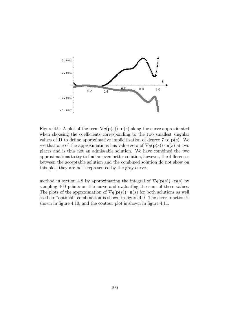
s

0.2 0.4 1.00.80.6

Figure 4.9: A plot of the term ∇q(p(s)) ·n(s) along the curve approximatedwhen choosing the coefficients corresponding to the two smallest singularvalues of D to define approximative implicitization of degree 7 to p(s). Wesee that one of the approximations has value zero of ∇q(p(s)) · n(s) at twoplaces and is thus not an admissable solution. We have combined the twoapproximations to try to find an even better solution, however, the differencesbetween the acceptable solution and the combined solution do not show onthis plot, they are both represented by the gray curve.

method in section 4.8 by approximating the integral of ∇q(p(s)) · n(s) bysampling 100 points on the curve and evaluating the sum of these values.The plots of the approximation of ∇q(p(s)) · n(s) for both solutions as wellas their ”optimal” combination is shown in figure 4.9. The error function isshown in figure 4.10, and the contour plot is shown in figure 4.11.

106

s

2. x 10-13

-2. x 10-13

1. x 10-13

-1. x 10-13

0.2 0.4

0.6 0.8 1.

Figure 4.10: The error of the approximation with a 7 degree algebraic curveto p(s) is varying-between −1.54× 10−13 and 1.98× 10−13 and is thus veryclose to the noise level of the digital representation with 16 digits accuracyused in the example. Because of this the plot has a ragged nature and thefirst and last points, which should be exactly at the zero line, are also affectedwith noise.

y

x

Figure 4.11: Contour plot of the 7th degree approximative implicitization ofp(s). By identifying the point (1, 1) in the plot and following the adjacentcurves to the point (6, 1) we recognize the shape of p(s). The plot showsthat regions where the expression ∇q(p(s)) · n(s) = 0, e.g. regions whereeither the curve normal is orthogonal to the gradient or where the gradientvanish are not too close to p(s).

107

Chapter 5

Approximation of IntersectionResults

A major challenge in the implementation of intersection algorithms is to rep-resent the intersections found in a proper way. In 3D CAD-systems boundarystructures are used to connect surfaces that describe the outer shell (and pos-sibly inner shells) of a volume. When making the union or intersection oftwo volumes, the first step is to intersect the shells of the volumes. Theintersection of the shells is performed by intersecting the surfaces composingthe shells. The curves from the surface intersections are then assembled in aproper way to trim away pieces of the surfaces no longer needed. Then newshells are built to describe the resulting volume object(s).The results of a surface surface intersection are points, curves and regions

of surfaces. The surface regions can be represented by a curve describing theboundary of the intersection region. The methods for the representation ofintersection curves are to a great extent based on piecewise cubic Hermiteinterpolation with GC1 or GC2 continuity between adjacent curve segments.Cubic Hermite interpolation is both used for 2D curves in the parameterdomain of the surfaces and for 3D curves. The most common intersectionrepresentations in CAD-systems are addressed in Section 5.1.When intersecting manifolds of higher dimension than two, we can expect

to get intersection results that must be described by manifolds of dimension2 or higher. A first choice is to resort to cubic Hermite interpolation definedover simplical domains of dimension d ≥ 2. However, the discussion inSection 5.2 shows that a piecewise local cubic Hermite interpolation oversimplical domains of dimension d ≥ 2 only has GC0 continuity betweenadjacent polynomial pieces. Thus, either higher degree Hermite interpolationhas to be employed or other approaches have to be found. One such approach,piecewise algebraic approximation in the parameter domain of the manifolds,

108

is discussed in Section 5.3. This approach can be based on the approximativeimplicitization, described in chapter 4.In Section 5.4 we address methods for approximation of algebraic repre-

sented manifolds, and give a general method that has the same convergencerate as the best approximation satisfying the same interpolation constraints.Tomodel the shape of the approximation the methodmakes use of the degreesof freedom remaining in the polynomial interpolant, when the interpolationconstraints are satisfied. Special attention is given to Hermite approxima-tion of 2D curves in Chapter 6. These results are further elaborated on theapproximation of circle and ellipse segments in Chapter 7.

5.1 Intersection Representation within CAD

The mostly used intersections in 3D CAD-systems are:

• Curve curve intersection in IR2 and IR3.

• Curve surface intersection in IR3.

• Surface surface intersection in IR3.

Results of such intersections can be described as objects of the followingcategories:

• Intersection points (0-manifolds). These are represented as pointsin respectively IR2 and IR3, and as a points in the parameter domainof the manifolds (curves/surfaces) being intersected.

• Intersection curves (1-manifolds). These are traditionally approx-imated by parametric curves in IR3. In the parameter domains ofthe surfaces being intersected, the intersection curves are also approx-imated by parametric curves. In certain cases exact representation ofthe intersection curve is present:

— When the intersection of a curve and another manifold (curve,surface or volume) coincide over an interval of the curve.

— When the intersection is along a segment of a constant parameterline in the parameter domain of a surface. In these cases a segmentof the constant parameter line, is an exact representation. Theimage of the segment of the constant parameter line is an exact3D representation of the intersection curve.

109

— For certain intersection constellations of surfaces the intersectioncurve is a first or second degree algebraic curve. In geometric mod-elers based on algebraic surface representation, much energy havebeen put into developing algorithms identifying such situations.

Geometric Hermite interpolation is the standard method for approxi-mating intersection curves. [Sederberg:91], [Höllig:95] and [Höllig:96]can be consulted for the theoretical background of geometric Hermiteapproximation of intersection curves. In [Sederberg:91] it is pointedout that the algebraic degree of the intersection curve between twobicubic patches is a curve with implicit equation of degree 324. It isalso pointed out that a representation of such a parametric intersectioncurve, as an exact parametric equation, is non-existent.

• Intersection regions on surfaces (2-manifolds). Intersection regionsare traditionally not handled in CAD-systems, because traditional in-tersection algorithms only to a limited degree handle coincident regionsin two surfaces. In Chapter 2 we discussed the introduction of intersec-tion tolerances, and proposed an approach for representing intersectionregions.

The cubic Hermite interpolant is often represented in a Bernstein basis,and is thus a R-positive 1-manifold, see remark 13 on page 52 in Chapter3. Often more than one cubic Hermite segment is required to approximatean intersection curve within proper tolerances. Different strategies for deter-mining the segmentation of the Hermite approximation exist. Two of theseare:

• Bisection. Two points on the intersection curve are known. A Her-mite approximation of the intersection curve is made between thesepoints. If the approximation satisfies the accuracy and shape qualityrequirements the segment is accepted. However, if the approximationdoes not satisfy these requirements, the approximation problem is splitinto two subproblems by finding a point on the intersection curve ly-ing between the two end points. This new point is used to define twosubsegments. The bisection process is then performed on each of thesubsegments. More information on the bisection process can be foundin [Sederberg:91].

• Tracing/Marching. From a point p0 on the intersection curve determinea step length based on e.g. curvature estimates or a fixed step lengths. Find a point on the intersection curve by first moving a distance

110

equal to the step length s in the direction of the curve tangent t0 at p0.Then iterate onto the intersection curve by constraining the interationto:

— A plane that has t0 as normal vector and is located at a distances in the direction t0 from p0.

— A sphere with center at p0 and radius s.

If the iteration fails, reduce the step length until the iteration suc-ceeds. Approximate the curve segment found. If the approximationdoes not satisfy accuracy and shape requirements resort to bisection.In the SISL library, see [SISL:94], such a combined tracing and bisec-tion strategy is employed. The efficiency of the combined tracing andbisection strategy is dependent on finding good initial step lengths sto avoid bisection. However, too small initial step lengths increase thenumbers of segments that are required for approximating the intersec-tion curve within a given tolerance. A survey of tracing algorithmscan be found in [Krishnan:96] where also the main problems of trac-ing/marching algorithms are addressed:

1. Converging back to the curve.

2. Component jumping.

3. Inability to handle singularities and multiple branches.

The approximation methods to be used, are not addressed in detail inthis chapter. In the next chapter, Chapter 6, we address the approxi-mation of curves in IR2 and show that algebraic curves in the parameterdomain of a surface can be approximated with O(h6) accuracy by con-trolling the tangent lengths of the cubic Hermite interpolant.

5.2 Cubic Hermite Approximation of Inter-section Results

To ensure local GCr continuity of triangular polynomial patches in IR3, the-orem 9.1 on page 410 in [Hoschek:93] states that the total polynomial degreen has to satisfy n ≥ 4r + 1. Thus, to achieve GC1-continuity between twopatches we have to resort to polynomials of total degree 5. Thus, cubictriangular polynomial patches can only be joined with GC0 continuity. Cu-bic interpolation of manifolds of higher dimensions than two defined oversimplical domains, can similarly only be joined by GC0 continuity.

111

Another description of these limitations is:

• In the case of cubic interpolation of curves, the number of vertices arefour. Only two vertices are allocated to ensure GC0 continuity. Thetwo other vertices can be employed to ensure GC1 continuity.

• For surfaces in IR3 nine out of ten vertices are used for ensuring GC0

continuity. Thus, only one vertex remains and these remaining degreesof freedom are too few to ensure GC1 continuity.

• For volumes and higher dimensional manifolds, all vertices are locatedon the boundary. They are thus all dedicated to ensure GC0 continuity.

5.3 Algebraic Approximation of IntersectionResults

In CAGD-systems using parameterized surfaces, the main use of curves inthe parameter domain of surfaces is to describe the location of intersectioncurves in the surfaces. The curves in the parameter domain are further usedas building blocks in the process assembling trimming structures dedicated toremoving parts of the surfaces. One of the interrogation functions in CAGDsystems utilizing the trimming information is the function for deciding if apoint is on a trimmed surface or not.As we have mentioned earlier, curves in the parameter domain of a surface

in IR3 are in general approximated by 2D parametric piecewise polynomialcurves. Such approximations require, in the general case, huge amounts of co-efficients to be sufficiently accurate. It is also well known that the transfer oftrimmed surfaces between systems from different CAD-vendors is a complexissue. Comments of this problem can e.g. be found in [IVF:94] appendix 4,page 6. The main reason for this is that the CAD-vendors currently (in 1996)use somewhat different strategies for solving approximation problems relatedto trimming, and somewhat different strategies for trying to compensate forproblems resulting from the approximation of intersection curves.We analyze in this section the consequences of introducing algebraic rep-

resentation of curves in the parameter domain to perform trimming of para-metric represented surfaces. The current method for representing trimminginformation is used in most CAD-systems, and is part of the ISO-standardISO 10303 (STEP), “Product data representation and exchange”. Thus wecan not expect a new method to immediately replace the current method.However, it can be a supplement and possibly an alternative for internal

112

representation in the 3D CAD-systems. Another possibility is to use thealgebraic representation as an intermediate stage for making better approx-imations to curves in the parameter domain of surfaces.

Definition 71 Let p : Ω → IR3 be a parametric surface (2-manifold) inIR3 defined over the compact domain Ω ⊂ IR2 and let the trimming functionassociated with p be denoted τ . Where τ : Ω → IR and τ is C0—continuous.p is trimmed according to the following rules:

τ(s, t) < 0 =⇒ (s, t) is outside the domain of the trimmed surface.τ(s, t) > 0 =⇒ (s, t) is inside the domain of the trimmed surface.τ(s, t) = 0 =⇒ (s, t) is on the boundary or inside the domain

the trimmed surface.

Provided that trimming functions can be defined in an efficient and accu-rate way, just one evaluation of a trimming function is needed to determineif a point with known location in the parameter domain is outside a trimmedversion of the surface.

Lemma 72 Given p : Ω → IR3 a parametric surface defined over the com-pact domain Ω ⊂ IR2 with no parts trimmed away. Then any trimmingfunction associated with p satisfy

τ(s, t) ≥ 0, (s, t) ∈ Ω.

Proof. Definition 71 assures this result.The trimming function of a nontrimmed surface can be assigned a con-

stant positive value.

Example 73 In figure 5.1 we show an example of a typical trimming curvein the parameter domain of a (rational) parametric NURBS surface p ofpolynomial orders (k1, k2). Assuming that a trimming curve is a result of theintersection of a parametric surface of orders (k1, k2) and an algebraic surfaceof total degree m, then the trimming curve can be described by a piecewisealgebraic curve of degrees (m(k1− 1),m(k2− 1)) in the parameter domain ofp.Thus if m = 2 and k1 = k2 = 4 the algebraic curves are described by a

tensor product B-spline function of degrees at most (6, 6). This results in atotal algebraic degree of 12 for the trimming curves.From Section 4.5 table 4.4 on page 81 we remember that for m = 3 the

convergence rate of the algebraic approximation to a rational Bernstein basisrepresented parametric surface is O(h5). We can expect that approximating

113

Figure 5.1: An example of a trimming curve and the segmentation of theparameter domain of the surface into a piecewise algebraic trimming function.Assuming that the surface to be trimmed is a NURBS surface, we can basethe initial grid on the knot vectors of the NURBS surface and subdivide eachmesh as required by the representation into triangular and rectangular parts.

a subset of a NURBS surface with degree 3 algebraic surfaces and then in-tersecting this approximation with another NURBS surface, results in fairlygood approximations of the trace of the intersection curve. For m = 3 andk1 = k2 = 4 we get algebraic curves of degrees (9, 9) given a total degree of18.

Lemma 74 Given p : Ω → IR3 a parametric surface defined over the com-pact domain Ω ⊂ IR2. Let pτ1 be p with the trimming function τ 1(s, t)assigned and let pτ2 be p with the trimming function τ 2(s, t) assigned. Then

pτ1 ∩ pτ2 ⊆ pτ1τ2 .

Proof.

pτ1 ∩ pτ2 = p(s, t) | τ 1(s, t) ≥ 0 ∧ τ 2(s, t) ≥ 0⊆ p(s, t) | τ 1(s, t)τ 2(s, t) ≥ 0 = pτ1τ2.

The consequence of the lemma is that to perform a stepwise trimmingoperation just by multiplication of trimming functions, is not straight for-ward. Phantom regions can appear in addition to a significant increase in thepolynomial degree of the trimming functions. In addition singular points are

114

Classification Inside τ 1 Partly inside τ 1 Outside τ 1Inside τ 2 Inside Use τ 1 OutsidePartly inside τ 2 Use τ 2 Detailed analyses OutsideOutside τ 2 Outside Outside Outside

Table 5.1: Classification of the possible trimming result when two trimmingfunctions τ 1(s, t) and τ 2(s, t) are applied to a subset of the parameter domainof a parametric surface.

introduced at points where algebraic curves from different trimming functionsmeet. Thus to base the trimming on products has a number of disadvantages.Since we deal with NURBS surfaces or rational Bezier surfaces it is nat-

ural to use a piecewise polynomial description of the trimming functions overthe parameter domain Ω. By doing so, we can subdivide a region to enabledescription of a trimming function combining two existing trimming func-tions. The first level of piecewise subdivision can be to use the subdivisionresulting from the piecewise description of the surface. In figure 5.1 the rec-tangular grid can typically originate from the original piecewise description ofa NURBS surface. When making the trimming functions over the subregionsof Ω, we come up with the cases described in table 5.1. We see from thistable that only the case where a subregion is partly inside both the trimmedsurfaces described by respectively τ 1(s, t) and τ 2(s, t), a detailed analyzeshas to be performed.In this case we have basically three situations:

• The algebraic curves described by τ 1(s, t) = 0 and by τ 2(s, t) = 0 don’tintersect in the subregion. Subdivide the subregion such that the curveτ 1(s, t) = 0 is in one part, and τ 2(s, t) = 0 is in another part.

• The algebraic curves described by τ 1(s, t) = 0 and by τ 2(s, t) = 0intersect in the subregion in a single point. Make a subdivision throughthe intersection point such that the piece of τ 1(s, t) = 0 to be used inthe combined trimming is in one part, and the piece of τ 2(s, t) = 0 tobe used in the combined trimming is in another part.

• More than one intersection point exist between τ 1(s, t) = 0 and τ 2(s, t) =0 in the subregion. Subdivide to separate single intersection points andpossibly coincidence between the curves into separate parts.

To make the continuity requirements on the trimming functions less re-strictive, by requiring that the trimming functions are C0 inside the sub-regions, but to allow jumps between subregions, we get an efficient way of

115

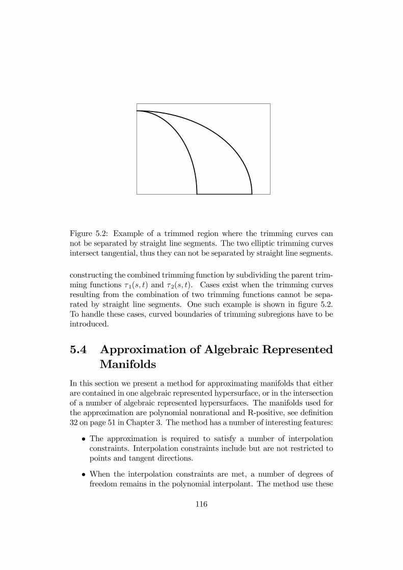
Figure 5.2: Example of a trimmed region where the trimming curves cannot be separated by straight line segments. The two elliptic trimming curvesintersect tangential, thus they can not be separated by straight line segments.

constructing the combined trimming function by subdividing the parent trim-ming functions τ 1(s, t) and τ 2(s, t). Cases exist when the trimming curvesresulting from the combination of two trimming functions cannot be sepa-rated by straight line segments. One such example is shown in figure 5.2.To handle these cases, curved boundaries of trimming subregions have to beintroduced.

5.4 Approximation of Algebraic RepresentedManifolds

In this section we present a method for approximating manifolds that eitherare contained in one algebraic represented hypersurface, or in the intersectionof a number of algebraic represented hypersurfaces. The manifolds used forthe approximation are polynomial nonrational and R-positive, see definition32 on page 51 in Chapter 3. The method has a number of interesting features:

• The approximation is required to satisfy a number of interpolationconstraints. Interpolation constraints include but are not restricted topoints and tangent directions.

• When the interpolation constraints are met, a number of degrees offreedom remains in the polynomial interpolant. The method use these

116

remaining degrees of freedom to model the shape of the approximation.This is done in such a way that the convergence rate is the same as forthe best approximation method using the same polynomial basis andsatisfying the same interpolation constraints.

• By doing numeric experiments with the method, the approximationrate of the best approximation with a given polynomial basis and giveninterpolation constraints can be found.

• The method can be used on manifolds contained in a single algebraichypersurface, or manifolds contained in the intersection of a number ofalgebraic hypersurfaces.

• The method is based on finding the minimum of the square sum ofthe coefficients of the combination q(pv(s)) of pv(s), the manifold usedfor the approximation, and the algebraic hypersurface q(x) = 0 beingapproximated. If the algebraic description of the manifold being ap-proximated is contained in the intersection of a number of algebraichypersurfaces qi(x) = 0, i = 1, . . . , g, then we minimize the sum ofthe square sum of all the coefficients of all combinations qi(p(s)). Weassume that all combinations qi(p(s)) are expressed in a PosProd basis.

The next step is to describe the manifold used in the approximation. Sincewe shall require interpolation of several points, and allow for the interpolationof tangents, we call this manifold an interpolant.

Description of Interpolant. In definition 32 on page 51 in Chapter 3 wedescribed the R-positive manifold of dimension g. We here address thenonrational variant, and thus describe the interpolant by the R-positivemanifold

p(s) =Xi∈In

ciBi,n(s), s ∈Ω.

Here Bi,n(s), i ∈ In are polynomial PosProd basis functions of degreen.

To approximate a manifold of dimension g, we require the interpolationof at least g + 1 linearly independent points. In addition to the pointsbeing interpolated, we can allow for the interpolation of a number oftangent directions and expressions dependent on higher order partialderivatives. The remaining degrees of freedom, when the interpolationconstraints are satisfied, we denote v. Thus the interpolant can beexpressed as

pv(s) =Xi∈In

ci(v)Bi,n(s), s ∈Ω. (5.1)

117

The combination of an algebraic hypersurface q(x) = 0 (of total degreem) and pv(s) can, because we only address nonrational approximation, havea simpler expression than in (4.3). Adapted to the notation of this sectionwe get the description

q(pv(s)) = (Dvb)T B(s), (5.2)

where B(s) contains all PosProd basis functions resulting from making them-th power of the PosProd basis described by Bi,n(s), i ∈ In. We haveintroduced Dv to express the dependence of the matrix D on the remainingdegrees of freedom in the interpolant. The number of basis function in B(s)is as before denoted Nmn.Since we know the algebraic hypersurface(s), the coefficient vector b is

constant. However, we want to combine Dv and b to d(v) = Dvb. Thus wereformulate (5.2) to

q(pv(s)) = d(v) ·B(s). (5.3)

We divide the further discussion in two parts addressed in separate sub-sections.

• In subsection 5.4.1 we address the approximation of a region of a man-ifold of dimension g ≤ (l − 1) in IRl lying in one algebraic representedhypersurface q(x) = 0.

The main result is a theorem stating that the convergence rate is thesame as for best approximation based on pv(s) when the approximationis based on minimizing kd(v)k2 with respect to v.We concluded with a corollary addressing the case g = l − 1. Thusaddressing the approximation of a (l − 1) dimensional manifold in IRl

lying in an algebraic represented hypersurface. For l = 2 this is theapproximation of algebraic represented curves in IR2. This is furtherdetailed in Chapter 6. For l = 3 this is the approximation of algebraicrepresented surfaces in IR3.

• In subsection 5.4.2 we address the approximation of a part of a manifoldof dimension g < (l − 1) lying in the intersection of (l − g) algebraicrepresented hypersurfaces in IRl. Setting g = 1 and l = 3 we have theapproximation of an algebraic curve in IR3.

We have split the discussion into these two parts, because the handling ofa single hypersurface is simpler than the handling the intersection of multiplehypersurfaces. Thus the discussion in Section 5.4.1 is more easy going thanthe discussion in Section 5.4.2.

118

5.4.1 Approximating Manifolds Contained in an Alge-braic Represented Hypersurface

The approximation method to be analyzed is based on finding the value(s)of v that gives kd(v)k2, defined in (5.3), its minimum value. The proof ofthe convergence rate for this method is divided in the following steps:

• First we give lemma 75 stating that when given:

— A manifold f of dimension g in IRl with g < l.

— An algebraic represented hypersurface q(x) = 0 containing f .

— An approximation method pv to f with convergence rate O(hr).

Then the combination q(pv(s)) has coefficients d(v) = O(hr).

• Then lemma 76 states that coefficients d(v) satisfy

|q(pv(s))| ≤ kd(v)k2 .

This indicates that minimizing kd(v)k2 can give an approximation toa part of the algebraic hypersurface q(x) = 0.

• Theorem 77 states that, given the above mentioned manifold f andthe existence of the O(hr) approximation, then the minimization ofkd(v)k2 is an O(hr) approximation provided:

— The gradient of q is nonvanishing close to f .

— The gradient of q is not orthogonal to the directions for errormeasurement close to f .

The direction for error measurement depends on the actual approxima-tion pv. Thus it is necessary to check if these conditions are satisfiedwhen an approximation has been found.

• This subsection is concluded by corollary 78 giving additional condi-tions simplifying the use of the approximation method in certain cases.These simplifications are:

— g = l − 1, i.e. approximating a part of a hypersurface.— Limit the variation of ∇q to be less than π

2close to f .

— Use ∇q(f(s)) as direction for error measurement.

119

Now we take the first step in the above mentioned process, and provethe convergence rate for the coefficient of the combination of the algebraicrepresented hypersurface, and the existing approximation method.

Lemma 75 Given a manifold f(t) of dimension g < l in IRl, an algebraichypersurface q(x) = 0 containing f and an approximation method pv(s), thatfor v = v, has an O(hr) convergence to f(t) for h small enough. Then for hsmall enough

kd(v)k∞ = O(hr)

withk(x1, . . . , xn)k∞ = max

i=1,...,n|xi| ,

where d(v) is given in (5.3).

Proof. Since we know we have an approximation pv with convergence rateO(hr) when v = v, we can decompose pv as follows

pv(s) = f(ϕ(s))+η(s)g(s),

where η(s) =O(hr) is the error function, the direction for error measurementg(s) satisfy kg(s)k2 = 1 and ϕ(s) a reparametrization.. By the assumption inthe lemma, we know that q(f) ≡ 0, and thus Taylor expansion with respectto η(s) gives (φ(s) replaces η(s) in the error term)

q(pv(t)) = q(f(ϕ(s)) + η(s)g(s)) (5.4)

= q(f(ϕ(s))+∇q(f(ϕ(s)) + φ(s)g(s)) · g(s)η(s)= ∇q(f(ϕ(s)) + φ(s)g(s)) · g(s)η(s)

with |φ(s)| ≤ |η(s)|. This Taylor expansion is the same as the one used onpage 82 to make (4.26). Combining this with (5.3), we get

d(v) ·B(s) = ∇q(f(ϕ(s)) + φ(s)g(s)) · g(s)η(s),

and introducing absolute values we get

|d(v) ·B(s)| ≤ maxs∈Ω

|∇q(f(ϕ(s)) + φ(s)g(s))| |η(s)| = O(hr).

Since the entries in B(s) are linearly independent and independent of h,entries in d(v) that have a convergence less than O(hr), can not be canceledby another entry. Thus for |d(v) ·B(s)| to be O(hr) all entries in d(v) haveto be O(hr), giving

kd(v)k∞ = O(hr).

120

The step following is to limit the value of |q(pv(t))| by kd(v)k2. Thusindicating the possibility to approximate a part of q(x) = 0 by minimizingkd(v)k2.

Lemma 76 Given f , q(x) = 0 and pv(s) as described in lemma 75, then

|q(pv(t))| ≤ kd(v)k2 .

Proof. From (5.3) we have that q(pv(s)) = d(v) ·B(s) with B(s) a PosProdbasis. Now we have that

|q(pv(s))| = |d(v) ·B(s)| ≤ kd(v)k∞ ≤ kd(v)k2 .

Now the foundation for proving the convergence rate is established.

Theorem 77 Given f , q(x) = 0 and pv(s) as described in lemma 75 andpv(s) defined by

kd(v)k2 = minv kd(v)k2 . (5.5)

If the gradient of q is nonvanishing and not normal to the directions for errormeasurement g(s) close to f(t), then for h small enough, the approximationmethod pv(s) has convergence rate O(hr). The approximation error is limitedby

|η(s)| ≤ mins ∈ Ω

|ρ| ≤ |η(s)|

kd(v)k2|∇q(f(ϕ(s)) + ρg(s)) · g(s)| . (5.6)

Proof. We can decompose pv in the same way as pv was decomposed in(5.4)

pv(s) = f(ϕ(s))+η(s)g(s),

givingq(pv(s)) = ∇q(f(ϕ(s)) + φ(s)g(s)) · g(s) η(s)

with η(s) being the approximation error. Since the gradient of q is nonvan-ishing and not normal to the direction for error measurement g(s) close to f ,we have for h small enough a region with ∇q(f(ϕ(s)) + φ(s)g(s)) · g(s) 6=0.Thus we have using lemma 76 and (5.5) that

121

|η(s)| = |q(pv(s))||∇q(f(ϕ(s)) + φ(s)g(s)) · g(s)|

≤ kd(v)k2mins ∈ Ω

|ρ| ≤ |η(s)|

|∇q(f(ϕ(s)) + ρg(s)) · g(s)|

≤ kd(v)k2mins ∈ Ω

|ρ| ≤ |η(s)|

|∇q(f(ϕ(s)) + ρg(s)) · g(s)|

= O(hr).

We now give a corollary, where the dimension g of the manifold, is set to(l − 1), thus covering:

• Approximation of algebraic represented curves in IR2.

• Algebraic represented surfaces in IR3.

Corollary 78 Given f , q(x) = 0, pv(s) and pv(s) as described in theorem77, and let the dimension of the manifold f be (l − 1). Let the directionfor error measurement at g(s) be parallel to ∇q(f(s)) and let the gradient ofq vary less that π

2close to f . Then for h small enough pv(s) is an O(hr)

approximation to f .

Proof. With the choice of g(s) parallel to the gradient, and the limitationof the variation of the gradient direction we have that close to f

min |∇q(f(ϕ(s)) + φ(s)g(s) · g(s)| 6= 0,

and theorem 77 gives |η(s)| = O(hr).

5.4.2 Approximation of Manifolds in the Intersectionof Algebraic Represented Hypersurfaces

The approximation problem to be addressed now is closely related to theproblem addressed in the previous subsection. The main difference is thatthe manifold f ∈ IRl now lies in the intersection of several hypersurfaces.

122

The notation is thus slightly more complicated. The minimization has to beperformed over a sum of the square sums of coefficients.We still let the dimension of f be denoted g, and denote the manifolds

intersecting along f by

qi(x) = 0, i = 1, . . . , l − g

with g < l − 1. The expression we want to minimize is

l−gXi=1

kdi(v)k22 (5.7)

with di(v) given by

qi(pv(s)) = di(v) ·B(s), i = 1, . . . , l − g. (5.8)

Here pv(s) is the interpolant given in (5.3).The main challenge is to find conditions that ensure that the minimiza-

tion of (5.7) results in an approximation with the required convergence rate.The proof of the convergence rate in theorem 77 did not use the dimension ofthe manifold being approximated, thus the results are also valid for this ap-proximation problem. For manifolds lying in the intersection of two or morehypersurfaces it is not difficult to construct examples where the directionof error measurement and the gradient of one of the manifolds, are normal.Thus the direction of error measurement can not be used with respect to allalgebraic hypersurfaces.To discuss the convergence rate of this approximation method we use a

similar structure of lemmas and theorems as in the previous section.

• First we give lemma 79, stating that when given:

— A manifold f of dimension g in IRl with g < l − 1.— Algebraic represented hypersurface qi(x) = 0, i = 1, . . . , g inter-secting along f .

— An approximation method pv to f with convergence rate O(hr).

Then the coefficients di(v) in (5.8) satisfy

gXi=1

kdi(v)k22 = O(hr).

123

• Theorem 80 then following states that the minimization ofPg

i=1 kdi(v)k22

gives an O(hr) approximation to f provided that:

— The gradient of one of the hypersurfaces qi(x) = 0, , i = 1, . . . , gis nonvanishing and not orthogonal to the direction for error mea-surement close to f .

The direction for error measurement is dependent on the actual ap-proximation pv. Thus, as in the case of one algebraic hypersurface,it is necessary to check the direction for error measurement after anapproximation has been found.

By adding the two following requirements to the hypersurfaces, we geta simpler approximation problem to implement:

— The gradient of qi, i = 1, . . . , g is nonvanishing close to f andvarying less than π

2close to f , for i = 1, . . . , g.

— The intersection of the hypersurfaces qi(x) = 0, i = 1, . . . , g isnonsingular along f .

Lemma 79 Given a manifold f(t) of dimension g < l − 1 in IRl, and aset of algebraic hypersurfaces qi(x) = 0, i = 1, . . . , l − g intersecting alongf . In addition assume that there exists an approximation method pv(s) thatfor v = v has an O(hr) convergence to f(t) for h small enough. Then for hsmall enough we have

max kdi(v)k∞ = O(hr), i = 1, . . . , l − g,

where di(v) is given in (5.8).

Proof. Since pv(s) is an approximation to the intersection of all the hyper-surfaces and have convergence rate O(hr), pv(s) it is also and approximationto each of the hypersurfaces. Thus lemma 75 can be used on each hypersur-face thus proving this lemma.Now we connect the convergence of the coefficients of the existing approx-

imation method to coefficients of the method based on the minimum squaresum.

Theorem 80 Given f , q and pv(s) as described in lemma 79. Let pv(s) bedefined by

l−gXi=1

kdi(v)k22 ≤ minv

l−gXi=1

kdi(v)k22 .

124

If for at least one j ∈ 1, . . . , g the gradient of qj is nonvanishing and notnormal to the directions for error measurement g(t) close to f(t), then forh small enough the approximation method pv(s) has convergence rate O(hr).The approximation error is limited by¯

ηj(s)¯≤ kdj(v)k2

mins ∈ Ω

|ρ| ≤¯ηj(s)

¯ |∇qj(f(ϕ(s)) + ρg(s)) · g(s)| .

Proof. Since the gradient of qj is nonvanishing and not normal to thedirections for error measurement g(t) close to f(t), the condition of theorem77 are satisfied giving¯

ηj(s)¯≤ kdj(v)k2

mins∈Ω,|ρ|≤|ηj(s)|

|∇qj(f(ϕ(s)) + ρg(s)) · g(s)| .

Further the definition of v and lemma 79 give

kdj(v)k2 ≤

vuut l−gXi=1

kdi(v)k22 ≤

vuut l−gXi=1

kdi(v)k22 = O(hr).

Thus the theorem is proved.

Remark 23 This theorem is difficult to put in practice, because the hyper-surfaces intersecting along f can have a singular intersection. Another prob-lem is that the gradients of the hypersurfaces can vanish, or vary more thandesirable. Thus to get a method that is simpler to implement, we add thefollowing conditions on hypersurfaces intersecting along f :

• For all i = 1, . . . , l− g the gradient of qi is required to be nonvanishingand vary less than π

2close to f .

• The intersection of the hypersurfaces qi, i = 1, . . . , g is nonsingularalong f .

Example 81 In [Höllig:95] theorem 3 states that: “For a smooth curve withnonvanishing curvature and torsion the error of the cubic geometric inter-polant is of order O(h5), where h is the length of the curves segment betweens0 and s1.” Here s0 and s1 are references to the parameter interval on thecurve f to be interpolated. The interpolation constraints imposed are interpo-lation of position and tangent direction at s0 and s1. Thus the interpolant can

125

be described as p(l0,l1)(s). The remaining degrees of freedom are the tangentlengths at the start and end of the cubic Hermite segment l0 and l1.Now assume that f lies in the nonsingular intersection of two algebraic

surfaces q1(x) = 0 and q2(x) = 0. Let d1(l0, l1) and d2(l0, l1) be defined as in(5.8). Then minimizing

kd1(l0, l1)k22 + kd2(l0, l1)k22

gives an O(h5) approximation, provided the resulting direction for error mea-surement satisfies the conditions in theorem 80.Thus using the algebraic implicitization with algebraic degree at least 2

in Chapter 4, and the approximation method of this section, enable us toapproximate f with O(h5) convergence, provided f has nonvanishing curvatureand torsion.If the torsion is vanishing all along the curve, then the curve is planar,

and the results from approximation of curves in IR2 can be used.

126

Chapter 6

Cubic Hermite Approximationof 2D Curves

When approximating the trace of an intersection curve in the parameterdomain of a parametric surface, it is desirable to find an approximation thatuse as few polynomial segments as possible. Constraints imposed on suchapproximations, are often a given polynomial degree and a maximum errorallowed.In this chapter we look at cubic Hermite approximation of curves in IR2

with O(h6) convergence. The basis for the methods presented is the theoremin [de Boor:87-2] where it is stated:“If f is a smooth curve with nonvanishing curvature and

h := sup |ti+1 − ti|

is sufficiently small, then the positive solution of the system (Q) exist andthe corresponding interpolant(s) pf satisfy dist(f, pf) = O(h6).”In this theorem the system (Q) describes the interpolation of position,

tangent and curvature from a planar curve f : IR→ IR2 at parameter valuesti and ti+1. The interpolant pf is a cubic Hermite interpolant. Tangentlengths at the start and end of the Hermite interpolant are controlled toachieve the required interpolation of curvature.Based on this we see that, provided the curvature is nonvanishing, and

the approximation is performed by a proper method, we can expect an O(h6)approximation to the curves in the parameter domain of a parametric surfaceby cubic Hermite interpolation.In Section 5.3 we pointed out that the trace of an intersection curve in the

parameter domain of a surface, is an algebraic curve. Thus, there is in generalno parametric description of such 2D curves. However, we have the algebraicrepresentation of the curve q(x, y) = 0 either as an exact representation or

127

as an approximation. The algebraic description gives the advantage that wehave a description independent of the parametrization of the curve. Thereis, however, a difficulty as well. From the algebraic representation and twopoints lying on the algebraic curve, we have no guarantee that the points lieon the same branch of the algebraic curve.The discussion in this chapter is structured as follows:

• In Section 6.1 we address approximation when both the parametric andalgebraic description of the curve is known. We use the convergencerate cited above for cubic Hermite interpolation of parametric curves inIR2 in combination with the algebraic representation of the curve. Thiscombination enables us to find Taylor expansions of the free tangentslengths of the cubic Hermite interpolant that give O(h6) convergence.The expansion is based on the parametrization of the curve to be ap-proximated.

• In Section 6.2 we address approximation when only the algebraic rep-resentation of the curve is known. We give a result being a consequenceof theorem 77 on page 121 in Section 5.3. Minimizing the square sumof the coefficients of the combination q(p(t)) is shown to give an O(h6)approximation. When using this method, the explicit parametric rep-resentation of the segment to be approximated, can be unknown.

• Finally in Section 6.3, we combine the approximative implicitizationin Chapter 4 and the above mentioned method for approximation ofalgebraic curves, to describe a two step approach to the approximationof parametric curves in IR2.

6.1 Power Expansion Based on ParametricRepresentation

Let an algebraic curve be defined by

q(x, y) = 0, (6.1)

whereq(x, y) =

Xi1+i2+i3=mi1,i2,i3≥0

ai1,i2,i3xi1yi2,

and letf(θ) = (fx(θ), fy(θ)), θ ∈ [−

α

2,α

2] (6.2)

128

be an exact parametric representation of a segment with nonvanishing cur-vature of the algebraic curve. We want to make a cubic Hermite interpolantp to q(x, y) = 0 satisfying

p(0) = f(−α2)

p0(0) k f 0(−α2) (6.3)

p(1) = f(α

2)

p0(1) k f 0(α

2),

where k means parallel to.

Description of interpolant. The Hermite interpolant p(t) is described ina cubic Bernstein basis

p(t) = (x(t), y(t)) =3X

i=0

pi

µ3

i

¶(1− t)3−iti, (6.4)

where

p0 =

µx0y0

¶=

µfx(−α

2)

fy(−α2)

¶p1 =

µx1y1

¶=

µfx(−α

2)

fy(−α2)

¶+ L0(α)

µf0x(−α

2)

f0y(−α

2)

¶p2 =

µx2y2

¶=

µfx(

α2)

fy(α2)

¶− L1(α)

µf0x(

α2)

f0y(

α2)

¶p3 =

µx3y3

¶=

µfx(

α2)

fy(α2)

¶.

Sincep(0) = p0 = f(−α

2)

p0(0) = 3(p1 − p0) = 3L0(α)f0(−α

2)

p0(1) = 3(p3 − p2) = 3L1(α)f0(α2)

p(1) = p3 = f(α2),

this interpolant satisfies the interpolation requirements in (6.3).

The problem is finding L0(α) and L1(α) such that p approximates f(θ)with accuracy O(α6). The procedure is divided in the following four steps:

129

1. In lemma 82 we establish an equation combining the algebraic curveq(x) = 0 with the Hermite interpolant p(t). This combination is apolynomial q(p(t)) of degree 3m, and is represented in a Bernsteinbasis.

2. In lemma 83 we show that there exists interpolants p such that thecoefficients of q(p(t)) have O(α6) convergence provided the curvatureof the segment approximated is nonvanishing.

3. Then in lemma 84 we establish a relation between the coefficients withconvergence rate O(α6) and the error of the Hermite interpolant. Hereit is required that the gradient of q is nonvanishing and not orthogo-nal to the direction for error measurement close to the curve segmentapproximated.

4. In theorem 85 we prove that O(α6) approximations can be found byTaylor expanding the coefficients found in lemma 82 and forcing allterms of degree less than 6 to be zero.

Lemma 82 Let the algebraic curve q(x) = 0, be defined as in (6.1) and letthe cubic Hermite interpolant p(t) be defined as in (6.4). Then the combina-tion of q(x, y) and p(t) can be written in the form

q(p(t)) =3m−2Xk=2

gk(α)

µ3m

k

¶(1− t)3m−ktk, (6.5)

for certain coefficients gk(α).

Proof. Since p(t) is a parametric cubic curve and q(x) = 0 is of degree m,then q(p(t)) is of degree 3m and thus can be described as in (6.5). But withthe index k in the sum going from 0 to 3m. The zero values of gk(α) fork = 0, 1, 3m− 1, 3m follow from (6.3).

Lemma 83 Let gk(α), k = 2, . . . , 3m − 2 be defined as in lemma 82, letas in (6.2) f(θ), −α

2≤ θ ≤ α

2be a segment with nonvanishing curvature of

the algebraic curve q(x, y) = 0 that we want to approximate. Then for αsufficiently small there exists p given in (6.4) such that the coefficients gk(α)satisfy

gk(α) = O(α6), k = 2, . . . , 3m− 2.

Proof. In [de Boor:87-2] it was shown that a cubic Hermite interpolantp(t) with O(α6) accuracy to a 2D curve segment f(θ) exists when the curve

130

segment has nonvanishing curvature. Thus, there exist L1(α) and L2(α)such that the approximation error ρ(t) = O(α6). Now we decompose p(t) asfollows

p(t) = f(ϕ(t)) + ρ(t)gϕ(t), (6.6)

where ϕ(t), is a reparametrization. and the unit vector gϕ(t) is the directionfor error measurement at f(ϕ(t)). The next step is to Taylor expand the ex-pression q(p(t)) with respect to ρ(t). (Note that in addition to the functionsρ(t) and ϕ(t) we also introduce the function φ(t) in the error term of theTaylor expansion).

q(p(t)) = q(f(ϕ(t)) + ρ(t)gϕ(t))

= q(f(ϕ(t))) +∇q(f(ϕ(t)) + φ(t)gϕ(t)) · gϕ(t)ρ(t) (6.7)

= ∇q(f(ϕ(t)) + φ(t)gϕ(t)) · gϕ(t)ρ(t)

with |φ(t)| ≤ |ρ(t)|, ρ(t)φ(t) ≥ 0. Thus, we can limit |q(p(t))| as follows

|q(p(t))| ≤ k∇q(f(ϕ(t)) + φ(t)gϕ(t))k2 |ρ(t)| .

Since ρ(t) is O(α6) for α small enough and L1(α) and L2(α) chosen properly,we get

|q(p(t))| ≤ max|φ(t)|≤|ρ(t)|

k∇q(f(ϕ(t)) + φ(t)nϕ(t))k2 |ρ(t)| = O(α6).

By the definition of gk, k = 2, . . . , 3m − 2 in (6.5) we get gk = O(α6),k = 2, . . . , 3m− 2.

Lemma 84 Let gk(α), k = 2, . . . , 3m− 2 be defined as in lemma 83, let asin (6.2) f(θ), −α

2≤ θ ≤ −α

2be a segment with nonvanishing curvature of the

algebraic curve q(x, y) = 0 that we want to approximate. If the gradient ofq is nonvanishing and not orthogonal to the direction of error measurementclose to f(θ), θ ∈ [−α

2, α2] then

|ρ(t)| ≤ K k(g2(α), . . . , g3m−2(α))k∞with K a constant.

Proof. From (6.5) we have that

|q(p(t))| ≤ k(g2(α), . . . , g3m−2(α))k∞ .

In (6.7) we showed that

q(p(t)) = ∇q(f(ϕ(t)) + φ(t)gϕ(t)) · gϕ(t)ρ(t).

131

Since for α sufficiently small, min|σ|≤ρmax

|∇q(f(ϕ(t)) + σgϕ(t)) · gϕ(t)| 6= 0 we

get

|ρ(t)| ≤ |q(p(t))|min

|σ|≤ρmax|∇q(f(ϕ(t)) + σgϕ(t)) · gϕ(t)|

≤ k(g2(α), . . . , g3m−2(α))k∞min

|σ|≤ρmax|∇q(f(ϕ(t)) + σgϕ(t)) · gϕ(t)|

= K k(g2(α), . . . , g3m−2(α))k∞ .

Theorem 85 Let the algebraic curve be defined as in (6.1) by q(x) = 0, andlet f(ϕ) as in (6.2) be an exact parametric representation of a segment withnonvanishing curvature of the algebraic curve. Then for α small enough anO(α6) approximation to the algebraic segment of the type (6.4) can be foundby Taylor expanding

gk(α), k = 2, . . . , 3m− 2defined in (6.5), and forcing the terms of degree less than 6 to be zero.

Proof. Lemma 83 ensures that gk(α), k = 2, . . . , 3m−2 are O(α6). Thus, aTaylor expansion around α = 0 gives us conditions for determining the firstterms in the Taylor expansion of respectively L0(α) and L1(α). Lemma 84connects the O(α6) behavior to the approximation error.In Chapter 7 this approach is used to describe a family of cubic Hermite

ellipse and circle approximations methods that has O(α6) convergence andhas a specific Taylor expansion of the free tangent lengths L0(α) and L1(α).

6.2 Minimizing the Square Sum of the Coef-ficients

In the previous section we established how to make an O(α6) cubic Hermiteapproximation by expansion of the coefficients of q(p(t)) with respect to α.We now show that an O(α6) interpolant can be found by minimizing the sumof the square of the coefficients of q(p(t)). This is a specialization of theorem77 on page 121 in Section 5.3.The first step is a lemma limiting the value of |q(p(t))| by an expression

including the square sum of the coefficients q(p(t)). Then a theorem is given,proving that the convergence rate of this approximation is O(α6).

132

Lemma 86 Let q(x) and p(t) be respectively defined as in (6.1) and (6.4)then

|q(p(t))| ≤

vuut3m−2Xk=2

(gk(α))2. (6.8)

Proof. From (6.5) we have that

|q(p(t))| ≤ max0≤k≤3m

|gk(α)| ≤

vuut3m−2Xk=2

(gk(α))2

proving (6.8).The theorem following is minimizing (6.8) and proving that the result-

ing Hermite interpolant is O(α6). We now, instead of using gk(α), k =2, . . . , 3m − 2 to describe the coefficients of the combination q(p(t)), usegk(L1, L2), k = 2, . . . , 3m− 2. We do this to focus on the tangent lengths instead of the parametrization in the theorem to follow.

Theorem 87 Let q(x) and f(θ) be defined respectively as in (6.1) and (6.2)having nonvanishing curvature. Then the cubic Hermite curve p(t) given in(6.4) with tangent lengths given by L1 and L2 satisfying

3m−2Xk=2

³gk(L1, L2)

´2= min

L1,L2

3m−2Xk=2

(gk(L1, L2))2 (6.9)

is an O(α6) approximation to f(ϕ) for α sufficiently small, provided that thegradient of q is nonvanishing close to f .

Proof. For α small enough we know that an O(α6) Hermite approxima-tion p(t) exists. Let the tangent length in such an O(α6) approximation berespectively L1 and L2. By (6.9) we have

3m−2Xk=2

³gk(L1, L2)

´2≤

3m−2Xk=2

³gk(L1, L2)

´2.

We know from lemma 83

¯q(pL1,L2(t))

¯≤

vuut3m−2Xk=2

³gk(L1, L2)

´2.

133

Thus ¯q(pL1,L2(t))

¯≤

vuut3m−2Xk=2

³gk(L1, L2)

´2= O(α6).

Now we choose the direction for error measurement parallel to the gradientof q at p(t). By lemma 84 on page 131, we have since the gradient of q isnonvanishing close to f , that p(t) is an O(α6) approximation of f(ϕ).

Remark 24 Assuming that p(t) is the best O(α6) approximation, by this wemean the approximation with the smallest maximum error, we see that the co-efficient of q(p(t)) resulting from approximation established in theorem 87 islimited by the 2-norm of the coefficients of q(p(t)) of this best approximation.Thus, the approximation in theorem 87 is close to the best approximation.

Remark 25 Since the actual value of α is not involved in the minimizationprocess, the method can be used, if the segment of the algebraic curve hasa parametric description. This parametrization does not have to be explicit.We only have to be able to assign a unique parameter value to each point ofthe segment being approximated. We can find such a parametrization by thefollowing approach, assuming that the tangent direction of the curve segmentf to be approximated, is varying less than π.

• Let l be a straight line going through the start and the end of the curvesegment f to be approximated.

• Let q lie on the side of l opposite to f .

• Let q lie between the lines that are tangential to respectively the startand end of f .

By choosing q according to the constraints above, straight lines through qonly intersect f once, because we assume that f has nonvanishing curvature.The parametrization of a point on f can be chosen to be the rotation angle ofthe straight line through q, intersecting f in the given point.The consequence of this observation is that we can use the algorithm from

theorem 87 to make O(α6) approximations of segments of algebraic curves.

6.3 Cubic Hermite Approximation of Para-metric Curves

In corollary 49 on page 78 we established conditions for an O(h(m+1)(m+2)

2−1)

approximation of an algebraic curve q(x, y) = 0 to a parametric curve seg-ment g(s), s ∈ [0, 1]. Then in theorem 85 on page 132 and remark 25 above

134

we established conditions for a O(h6) cubic Hermite approximation p(t) toan algebraic curve q(x, y) = 0. Combining these results we obtain an al-gorithm for making an O(h6) cubic Hermite approximation of a segment ofparametric curve, by introducing an intermediate algebraic approximation ofdegree m ≥ 3.Let r(α), α ∈ [0, 1] be the exact representation of the segment of the alge-

braic curve used in the approximation. We then get the following separationof the errors of the two approximation stages

kp(t)− g(φ1(t))k2 ≤ kp(t)− r(φ2(t)) + r(φ2(t))− g(φ1(t))k2≤ kp(t)− r(φ2(t))k2 + kr(φ2(t))− g(φ1(t))k2≤ O(h

(m+1)(m+2)2

−1) +O(h6)

with φ2(t) and φ1(t) being reparametrization.For m = 1, 2, . . . we get the following total convergence rates

Algebraic degree 1 2 ≥3Convergence rate O(h2) O(h5) O(h6)

provided that conditions used for establishing these convergence rates incorollary 49 and theorem 85 are fulfilled. These conditions are:

• The gradient of q close to g(s) must be nonvanishing.

• The curvature of the segment of the intermediate algebraic curve usedmust be nonvanishing.

Example 88 In the first version of SINTEF Spline Library SISL tangentlengths for a Hermite segment approximating an intersection curve was es-timated by using position, tangent and radius of curvature at both start andend point.The tangent length L0 for the start point was calculated by assuming that

the curve was a circle with radius rstart and opening angle α using the tangentlength estimate given in example 96. Similarly the tangent length for the endL1 was estimated based on rend and α. The opening angle α was set to theangle between the start and end tangent.This method is in the general case at most an O(h5) approximation. How-

ever, if the curve happened to be a circle segment the approximation rate isO(h6). Some informal measurements that were performed on the convergencerate, showed that in many practical cases from 3D CAD an O(h5) behaviorwas observed. An unexpected consequence of the higher approximation rate

135

for circles was a bug report from a user stating that too few Hermite seg-ments were produced when marching intersection curves that were true circlesegments.

136

Chapter 7

Ellipse and CircleApproximation

In Chapter 6 we looked at cubic Hermite approximation of curves in IR2 andcited [de Boor:87-2] to establish O(h6) convergence for cubic Hermite inter-polation of curves with nonvanishing curvature. Ellipses are curves satisfyingthis curvature requirement. The paper introduced the first O(h6) circle in-terpolants. Then the paper [Dokken:90] introduced possibilities to model theshape of the error function by combining:

• The algebraic description of the circle being approximated.

• The parametric description of the cubic Hermite interpolant.

In the papers [Floater:95-1], [Floater:96] and [Floater:97] the followingaspects of conic approximation are respectively addressed:

• High order approximation by quadratic splines.

• Cubic approximation schemes for conic sections.

• O(h2n) Hermite approximation for conic sections.

In this chapter we use the idea from [Dokken:90] and combine it with theresults of theorem 85 in Chapter 6 applied to ellipse approximation. Theorem85 showed how we can utilize the algebraic and parametric description of acurve segment being approximated to control the cubic Hermite interpolationin such a way that O(h6) convergence is achieved.The first step in the analyzes of ellipse approximation is to give the de-

scription of the ellipse segment and the cubic Hermite interpolant. When

137

discussing circle approximation the natural circle to use is the unit circle.The area of a unit circle is π; the area of an ellipse is πab where a and b arethe half axis. By choosing the half axis to be b and 1

b, we have an ellipse with

the area of a unit circle. By scaling, translation and rotation any ellipses canbe derived from this “unit ellipse”. In addition for b ≡ 1 the “unit ellipse” isthe unit circle.

The Ellipse Segment. The ellipse segment is described by

c(θ) = (b cos θ,1

bsin θ), τ ≤ θ ≤ τ + α (7.1)

with b > 0. The algebraic description of the ellipse segment c(θ) isq(x, y) = 0 with

q(x, y) =³xb

´2+ (b y)2 − 1. (7.2)

Hermite Interpolant. The Hermite interpolant p(t) is required to matchposition and tangent of (7.1) for θ = τ and θ = τ +α. The descriptionof p(t) in a cubic Bernstein basis is:

p(t) = (x(t), y(t)) =3X

i=0

pi

µ3

i

¶(1− t)3−iti, (7.3)

where

p0 = c(τ) =

µb cos (τ)1bsin τ

¶p1 = c(τ) + L0(α)c

0(τ)

=

µb cos (τ)1bsin (τ)

¶+ L0(α)

µ−b sin (τ)1bcos τ

¶p2 = c(τ + α)− L1(α)c

0(τ + α)

=

µb cos (τ + α)1bsin (τ + α)

¶− L1(α)

µ−b sin (τ + α)1bcos (τ + α)

¶p3 = c(τ + α) =

µb cos (τ + α)1bsin (τ + α)

¶.

The only unknown quantities in p(t) are the tangent length descriptionsL0(α) and L1(α). The problem is thus to control L0(α) and L1(α) to get abest possible approximation.The parametric and algebraic description of the ellipse segment satisfy

the conditions of theorem 85. Thus, we can power expand the coefficient of

138

q(p(t)) with respect to α. We know that the terms of degree lower than 6vanish for proper choices of L0(α) and L1(α).We structure this chapter as follows.

• In Section 7.1 we give a theorem that states when L0(α) and L1(α)satisfy

L0(α) =α

3+

¡124+ c1

¢α3

6+

c2α4

24+O(α5) (7.4)

L1(α) =α

3+

¡124− c1

¢α3

6− c2α

4

24+O(α5), (7.5)

then the Hermite ellipse interpolant is O(α6). The theorem also givestwo alternative Taylor expansions with O(α6) convergence. However,these have a much larger approximation error.

For circle approximation it is natural to require L0(α) ≡ L1(α) to geta symmetric approximation. The section is concluded with a corollarystating that forcing L0(α) ≡ L1(α) results in

L0(α) = L1(α) =α

3+

α3

144+O(α5). (7.6)

• In Section 7.2 we give examples of circle approximation methods satis-fying (7.6).

• Examples of methods for ellipse approximation that satisfies (7.4) and(7.5) are then given in Section 7.3. The constants c1 and c2 are hereused to model the approximation to give a desired shape. Also higherdegree terms are added to (7.4) and (7.5) to give better shape control.

• We conclude the chapter in Section 7.4 by three O(h8) circle approxi-mations based on a fourth degree interpolant that match position andtangent direction at the segment ends.

7.1 Taylor Expansion of Tangent Lengths

We address in this section conditions on the Taylor expansion of the tangentlength functions to achieve O(α6) convergence. The discussion is structuredas follows:

• The first step is a lemma that express q(p(t)) in a 6-th degree Bernsteinbasis.

139

• Then the main result of this subsection is stated in theorem 90. Herethree different pairs of Taylor expansions of L0(α) and L1(α) are giventhat give an O(α6) convergence of the ellipse approximation.

• Then we discuss the error of these and conclude that the one referencedin (7.4) and (7.5) has the smallest error functions.

• In circle approximation, symmetry in the approximation is often re-quired, thus demanding that L0(α) ≡ L1(α). In corollary 91 we lookat this problem and deduct the tangent length function in (7.6).

To simplify the theorem to follow, we give the following lemma expressingq(p(t)) in a 6-th degree Bernstein basis.

Lemma 89 Let the Hermite interpolant p(t) to the ellipse segment be de-scribed as in (7.3) and let the algebraic description of the ellipse be q(x) = 0as describe in (7.2) then

q(p(t)) = 15a(α)(1− t)4t2 + 20b(α)(1− t)3t3 + 15c(α)(1− t)2t4, (7.7)

where

a(α) =3L0(α)

2 + 2L1(α) sinα− 2(1− cosα)5

b(α) =−9L1(α)L0(α) cosα+ 9(L1(α) + L0(α)) sinα− 10(1− cosα)

10

c(α) =3L1(α)

2 + 2L0(α) sinα− 2(1− cosα)5

.

(7.8)

Proof. Can be verified by expanding the expressions.The theorem following shows that three different pairs of Taylor expan-

sion exists for L0(α) and L1(α) that give an O(α6) convergence of the errorfunction.

Theorem 90 Let the cubic Hermite interpolant p(t) and the ellipse segmentc(α) be defined as in lemma 89. If the tangent length functions L0(α) andL1(α) satisfy either

L0(α) =α

3+

¡124+ c1

¢α3

6+

c2α4

24+O(α5)

L1(α) =α

3+

¡124− c1

¢α3

6− c2α

4

24+O(α5),

140

or

L0(α) =α

3+

1

2√3α2 +

¡−13+ c1

¢α3

6+

¡−√3c1 + c2

¢α4

24+O(α5)

L1(α) =α

3− 1

2√3α2 +

¡−13− c1

¢α3

6+

¡−√3c1 − c2

¢α4

24+O(α5),

or

L0(α) =α

3− 1

2√3α2 +

¡−13+ c1

¢α3

6+

¡√3c1 + c2

¢α4

24+O(α5)

L1(α) =α

3+

1

2√3α2 +

¡−13− c1

¢α3

6+

¡√3c1 − c2

¢α4

24+O(α5),

then the approximation p(t) to the ellipse segment is O(α6).The corresponding Taylor expansions of a(α), b(α) and c(α) defined in

(7.8) are respectively

a(α) =³

757600

+ 180c1 +

160c21 +

1300

³L(5)0 + L

(5)1

´´α6

+³

1320

c2 +1120

c2c1 +1

1800

³L(6)0 + L

(6)1

´´α7 +O (α8)

b(α) =³− 2338400

+ 140c21 +

1200

³L(5)0 + L

(5)1

´´α6

+³180c2c1 +

11200

³L(6)0 + L

(6)1

´´α7 +O (α8)

c(α) =³

757600

− 180c1 +

160c21 +

1300

³L(5)0 + L

(5)1

´´α6

+³− 1320

c2 +1120

c2c1 +1

1800

³L(6)0 + L

(6)1

´´α7 +O (α8) ,

and

a(α) =³

111800− 1

40c1 +

√3

120c2 +

160c21 +

1300

³L(5)0 + L

(5)1

´´α6

+³√

3180

c1 −√3

120c21 +

1120

c2c1 −√3

1800+

√3

600L(5)0 + 1

1800

³L(6)0 + L

(6)1

´´α7 +O (α8)

b(α) =³− 491200

+√380c2 +

140c21 +

1200

³L(5)0 + L

(5)1

´´α6

+³−7

√3

240c1 +

180c2c1 +

√3

800

³L(5)0 − L

(5)1

´+ 1

1200

³L(6)0 + L

(6)1

´´α7 +O (α8)

c(α) =³

111800

+ 140c1 +

√3

120c2 +

160c21 +

1300

³L(5)0 + L

(5)1

´´α6

+³√

3180

c1 +√3

120c21 +

1120

c2c1 +√3

1800−

√3

600L(5)1 + 1

1800

³L(6)0 + L

(6)1

´´α7 +O (α8) ,

141

and

a(α) =³

111800− 1

40c1 −

√3

120c2 +

160c21 +

1300

³L(5)0 + L

(5)1

´´α6

+³−√3

180c1 +

√3

120c21 +

1120

c2c1 +√3

1800−

√3

600L(5)0 + 1

1800

³L(6)0 + L

(6)1

´´α7 +O (α8)

b(α) =³− 491200−√380c2 +

140c21 +

1200

³L(5)0 + L

(5)1

´´α6

+³7√3

240c1 +

180c2c1 +

√3

800

³L(5)1 − L50

´+ 1

1200

³L(6)0 + L

(6)1

´´α7 +O (α8)

c(α) =³

111800

+ 140c1 −

√3

120c2 +

160c21 +

1300

³L(5)0 + L

(5)1

´´α6

+³−√3

180c1 −

√3

120c21 +

1120

c1c2 −√3

1800+

√3

600L(5)1 + 1

1800

³L(6)0 + L

(6)1

´´α7 +O (α8) .

Proof. Since we already know than an O(α6) approximation exists, we justhave to find conditions for L0(α) and L1(α) that ensure that the terms ofdegree 5 or lower in the Taylor expansion of a(α), b(α) and c(α) vanish. Theproof has the following steps:

• First we make the Taylor expansion with seven terms of a(α), b(α) andc(α). Here we notice that the only unknown expressions are derivativesof L0(α) and L1(α) up to order 5 for α = 0.

• Then we successively look at conditions that make the terms of degreefive or lower in the Taylor expansion a(α), b(α) and c(α) vanish.

Taylor expanding respectively a(α), b(α) and c(α) to 7 terms we get:

a(α) =¡35L0 (0)

2¢+ ¡65L0 (0)L

00 (0) +

25L1 (0)

¢α

+¡35L0 (0)L

000 (0) +

35L00 (0)

2 − 15+ 2

5L01 (0)

¢α2

+¡15L0 (0)L

0000 (0) +

35L00 (0)L

000 (0)− 1

15L1 (0) +

15L001 (0)

¢α3

+

¡− 115L01 (0) +

115L0001 (0) +

160+ 3

20L000 (0)

2

+15L00 (0)L

0000 (0) +

120L0 (0)L

(4)0 (0)

´α4

+

³110L000 (0)L

0000 (0) +

120L(4)0 (0)L00 (0) +

1100

L0 (0)L(5)0 (0)

+ 160L(4)1 (0) + 1

300L1 (0)− 1

30L001 (0)

´α5

+O(α6),

142

and

b(α) =¡− 910L1 (0)L0 (0)

¢+¡− 910L1 (0)L

00 (0)− 9

10L01 (0)L0 (0) +

910L1 (0) +

910L0 (0)

¢α

+

¡− 920L1 (0)L

000 (0)− 9

20L001 (0)L0 (0)− 9

10L01 (0)L

00 (0)

+ 920L1 (0)L0 (0)− 1

2+ 9

10L00 (0) +

910L01 (0)

¢α2

+

¡920L1 (0)L

00 (0) +

920L01 (0)L0 (0)− 3

20L1 (0)L

0000 (0)

− 920L01 (0)L

000 (0)− 3

20L0001 (0)L0 (0)− 9

20L001 (0)L

00 (0)

− 320L1 (0)− 3

20L0 (0) +

920L000 (0) +

920L001 (0)

¢α3

+

¡− 320L00 (0)− 3

20L01 (0) +

320L0000 (0) +

320L0001 (0) +

124

+ 940L1 (0)L

000 (0) +

940L001 (0)L0 (0) +

920L01 (0)L

00 (0)

− 380L1 (0)L0 (0)− 9

40L001 (0)L

000 (0)− 3

20L01 (0)L

0000 (0)

− 380L1 (0)L

(4)0 (0)− 3

80L(4)1 (0)L0 (0)− 3

20L0001 (0)L

00 (0)

´α4

+

³− 340L001 (0)L

0000 (0)− 3

80L(4)1 (0)L00 (0)− 3

400L1 (0)L

(5)0 (0)

− 380L01 (0)L

(4)0 (0)− 3

400L(5)1 (0)L0 (0)− 3

40L0001 (0)L

000 (0)

− 380L1 (0)L

00 (0)− 3

80L01 (0)L0 (0) +

340L1 (0)L

0000 (0)

+ 940L01 (0)L

000 (0) +

340L0001 (0)L0 (0) +

940L001 (0)L

00 (0)

+ 380L(4)1 (0) + 3

80L(4)0 (0) + 3

400L1 (0)

+ 3400

L0 (0)− 340L000 (0)− 3

40L001 (0)

¢α5

+O(α6),

and

c(α) =¡35L1 (0)

2¢+ ¡65L1 (0)L

01 (0) +

25L0 (0)

¢α

+¡35L1 (0)L

001 (0) +

35L01 (0)

2 − 15+ 2

5L00 (0)

¢α2

+¡15L1 (0)L

0001 (0) +

35L01 (0)L

001 (0)− 1

15L0 (0) +

15L000 (0)

¢α3

+

¡− 115L00 (0) +

115L0000 (0) +

160

+ 320L001 (0)

2 + 15L01 (0)L

0001 (0) +

120L1 (0)L

(4)1 (0)

´α4

+

³110L001 (0)L

0001 (0) +

120L(4)1 (0)L01 (0)

+ 1100

L1 (0)L(5)1 (0) + 1

60L(4)0 (0) + 1

300L0 (0)− 1

30L000 (0)

´α5

+O(α6).

Now we successively look at terms in the expansions of higher and higherdegree to establish conditions that make the terms of degree five or lower

143

vanish. First we look at the coefficients of the terms of degree zeroµ3

5L0 (0)

2

¶= 0µ

− 910

L1 (0)L0 (0)

¶= 0µ

3

5L1 (0)

2

¶= 0.

We see that only assigning L0 (0) = 0 and L1 (0) = 0 set the coefficients ofthe zero degree terms to 0. Remember these values for use later in the proof.The first degree terms are all zero by these assignments. The second degreeterms are reduced to µ

3

5L00 (0)

2 − 15+2

5L01 (0)

¶= 0µ

− 910

L01 (0)L00 (0)−

1

2+9

10L00 (0) +

9

10L01 (0)

¶= 0µ

3

5L01 (0)

2 − 15+2

5L00 (0)

¶= 0.

These equations only vanish when L00(0) = L01(0) =13. Now the third degree

terms are reduced to the condition

L000 (0) + L001 (0) = 0.

Further all the fourth degree terms are reduced to the condition

L0000 (0) + L0001 (0) =1

12− 94(L000 (0))

2,

and the fifth degree terms reduce to

6L000 (0)L0000 (0) + L

(4)0 (0) + L

(4)1 (0) + 2L000 (0) = 0

3L000 (0) (L0000 (0)− L0001 (0)) + L

(4)1 (0) + L

(4)0 (0) = 0

−6L000 (0)L0001 (0) + L(4)1 (0) + L

(4)0 (0)− 2L000 (0) = 0.

These three equations are linearly dependent, and we can substract the lastfrom the first to get:

L000 (0)

µL0000 (0) + L0001 (0) +

2

3

¶= 0.

144

Combining with the condition from the fourth degree terms, we get

L000 (0)

µ1

12− 94(L000 (0))

2+2

3

¶= 0,

resulting in

L000 (0) = 0 or L000 (0) = ±

1√3.

Above in the proof we have already found that

L0(0) = L1(0) = 0

L00(0) = L01(0) =1

3.

Analyzing the above three alternatives for L000 (0) , and applying these on theforth and fifth degree terms, we get remembering that L000(0) + L001(0) = 0 :

1. First alternative L000 (0) = L001 (0) = 0, giving the following requirements

L0000 (0) + L0001 (0) =1

12

L(4)0 (0) + L

(4)1 (0) = 0.

These are satisfied by

L0(α) =α

3+

¡124+ c1

¢α3

6+

c2α4

24

L1(α) =α

3+

¡124− c1

¢α3

6− c2α

4

24.

2. Second alternative L000 (0) =1√3and L001 (0) = − 1√

3, giving the following

requirements

L0000 (0) + L0001 (0) = −23√

3 (L0000 (0)− L0001 (0)) + L(4)1 (0) + L

(4)0 (0) = 0.

These are satisfied by

L0(α) =α

3+

1

2√3α2 +

¡−13+ c1

¢α3

6+

¡−√3c1 + c2

¢α4

24

L1(α) =α

3− 1

2√3α2 +

¡−13− c1

¢α3

6+

¡−√3c1 − c2

¢α4

24.

145

3. Third alternative L000 (0) = − 1√3and L001 (0) =

1√3, giving the following

requirements

L0000 (0) + L0001 (0) = −23

−√3 (L0000 (0)− L0001 (0)) + L

(4)1 (0) + L

(4)0 (0) = 0.

These are satisfied by

L0(α) =α

3− 1

2√3α2 +

¡−13+ c1

¢α3

6+

¡√3c1 + c2

¢α4

24

L1(α) =α

3+

1

2√3α2 +

¡−13− c1

¢α3

6+

¡√3c1 − c2

¢α4

24.

Higher order terms in L0(α) and L1(α) do not influence the annihilationof the low order terms, thus we can add a O(α5) term to the expansion ofL0(α) and L1(α).The Taylor expansions of a(α), b(α) and c(α) are now straight forward

by using the proper pairs of Taylor expansion of L0(α) and L1(α).Looking at the sixth order terms of the alternative Taylor expansions

of a(α), b(α) and c(α), we see that the constants in the first expansionare much smaller than in the other two, thus we prefer to concentrate theexamples in the next section on the first alternative. Tests have shown amuch smaller error function when using the first alternative compared tothe others. For circle approximation the first alternative is the one givingthe best approximation. In addition symmetry of tangent lengths for circleapproximation is impossible with the second and third alternative.In circle approximation it is natural to require symmetry of tangent length

and thus requiring L0(α) ≡ L1(α). The following corollary presents theconsequence of this simplification.

Corollary 91 Let the approximation problem be defined as in theorem 90and in addition impose that

L0(α) ≡ L1(α) ≡ L(α).

Then to achieve O(h6) convergence L(α) has to satisfy

L(α) =α

3+

α3

144+O(α5). (7.9)

In addition a(α) ≡ c(α). The Taylor expansion of a(α) and b(α) satisfy

a(α) = ( 757600

+ 1150

L(5)(0))α6 +O(α7) (7.10)

b(α) = (− 10338400

+ 292400

L(5)(0))α6 +O(α7). (7.11)

146

Circle approximation Example Inside error Outside errorSimplest 94 −6.6× 10−5 3.4× 10−6One sided outside 95 0 1.9× 10−5Equioccilating 96 −1.4× 10−5 1.4× 10−5Flat 98 0 6.2× 10−5Zero integral 100 −1.9× 10−5, 1.2× 10−5Minimum square sum 101 0 2.4× 10−5

Table 7.1: The table shows a summary of different cubic Hermit circle approx-imations and how the error behaves. The approximation with least variationof error is the “one sided outside” that has an error variation of 1.9× 10−5,the “equioccilating” has a variation in error 2.8× 10−5. The circle segmentapproximateded is a segment with opening angle 1 of a unit circle.

Proof. To get the required symmetry c1 = c2 = 0. This gives the Taylorexpansion of the tangent length function in (7.9). The Taylor expansion ofa(α) and b(α) is now straight forward.

7.2 Some Cubic Hermite Circle Interpolants

The background for the work on circle approximation methods described inthis section was accuracy requirements to the spline library SISL developedat SINTEF in Oslo in 1988-1989. The basic idea behind these methods isto model the shape of the error function of the cubic Hermit interpolants,and is described in [Dokken:90]. In [Moerken:91-2] Quadratic Interpolationof circles is addressed, while in [Lyche:94] these ideas are extended to odddegrees n and an error function e(t) = O(t2n). The goal in this sectionis to combine a required geometric shape in the error function and a highconvergence rate for cubic Hermite interpolants.In corollary 91 we addressed conditions to be imposed on the Taylor

expansion of the tangent length at the start and end of a cubic Hermit circleinterpolant to achieve O(α6) convergence. This is the basis for a family ofO(α6) circle interpolants. We illustrate the flexibility of this family by thefollowing examples:

• The near equioscillating Hermite circle approximation with two internalzeroes.

• The one sided circle approximation with a double zero in the middle.

147

• The circle approximation with simplest Taylor expansion of the tangentlength function.

• An O(α6) circle approximation with no internal zeroes.

• A circle approximation with zero integral of q(p(t)).

• A circle approximation with a minimum of the square of the Beziercoefficients of q(p(t)). Also in this there are no internal zeroes.

For a brief overview of the methods table 7.1 summarizes the error vari-ation of the methods. As usual with approximation methods, which methodis the best depends upon the actual use of the approximation.The Hermite interpolant we use, is described in (7.3). Since we have

L1(α) ≡ L2(α) ≡ L(α) as in corollary 91, we here get a somewhat simplerdescription of the Hermite interpolant than on page 138.

p(t) = (x(t), y(t)) =3X

i=0

pi

µ3

i

¶(1− t)3−iti, (7.12)

where

p0 = c(0) =

µ10

¶p1 = c(0) + L(α)c0(0) =

µ10

¶+ L(α)

µ01

¶p2 = c(α)− L(α)c0(α) =

µcosαsinα

¶− L(α)

µ− sinαcosα

¶p3 = c(α) =

µcosαsinα

¶.

In this case the expression q(p(t)) reduces to

q(p(t)) = 15a(α)(1− t)4t2 + 20b(α)(1− t)3t3 + 15a(α)(1− t)2t4,

where

a(α) = 15(3L(α)2 + 2L(α) sinα− 2(1− cosα)) (7.13)

b(α) = 110(−9L(α)2 cosα+ 18L(α) sinα− 10(1− cosα)). (7.14)

These values for a(α) and b(α) can also be found in [Dokken:90]. For theapproximation to be O(α6), corollary 91 stated that

L(α) =α

3+

α3

144+O(α5).

148

One requirement that has to be satisfied for the interpolant to be O(α6),was that the gradient of the algebraic curve must be nonvanishing close tothe curve being approximated. For a circle the gradient is only vanishing atthe circle center. Thus, imposing that 0 < α < π, and only allow positivevalues for L(α), keeps the approximation away from the origin.The algebraic description of the unit circle, that is used in this section,

is q(x, y) = 0 withq(x, y) = x2 + y2 − 1. (7.15)

Before giving examples, we give a theorem that connects the behavior ofq(p(t)) to the approximation error. The theorem also shows that the maxi-mum value of |q(p(t))|

2is a good error estimate for the circle approximations

to be used in the examples. When we say error function in the example inthis section, and in Section 7.4, we use this error estimate.

Theorem 92 Let the Hermite interpolant p(t) to the circle segment be de-scribed as in (7.12) and let the algebraic description of the unit circle q(x) = 0be described as in (7.15). Provided that the error

ρ(t) =px(t)2 + y(t)2 − 1

in the circle approximation satisfy

ρmax = max0≤t≤1

|ρ(t)| < 1, (7.16)

then

|ρ(t)| ≤ |q(p(t))|2(1− ρmax)

. (7.17)

Proof. The Hermite interpolant p(t) can be decomposed such that p(t) =p0(t) + ρ(t)n0(t), where q(p0(t)) = 0 is an exact representation of the circlesegment and n0(t) is the unit normal of the circle segment at p0(t). Usingthis decomposition and Taylor expanding to two terms with respect to ρ(t)we get

q(p(t)) = q(p0(t) + ρ(t)n0(t))

= q(p0(t)) +∇q(p0(t) + θ(t)n0(t)) · n0(t))ρ(t)= ∇q(p0(t) + θ(t)n0(t)) · n0(t))ρ(t).

Here θ(t)ρ(t) ≥ 0, |θ(t)| ≤ |ρ(t)|. We have that ∇q(p0(t) + θ(t)n0(t)) isparallel to n0(t), resulting in

|q(p(t))| = k∇q(p0(t) + θ(t)n0(t))k2 |ρ(t)| .

149

t 10.80.60.40.20

0.0001

0

-0.0001

Figure 7.1: Error of the simplest circle approximation with convergence rateO(α6). The circle segment approximated has opening angle α = 1 and unitradius.

Now assuming that ∇q(p0(t) + θ(t)n0(t)) 6= 0, we get

|ρ(t)| = |q(p(t))|k∇q(p0(t) + θ(t)n0(t))k2

. (7.18)

Going back to the definition of q(x) = 0 in (7.15), we get

∇q (p0(t) + θ(t)n0(t)) = 2n0(t)(1 + θ(t)).

Thusk∇ (p0(t) + θ(t)n0(t))k2 = 2 |1 + θ(t)| .

Since |θ(t)| ≤ |ρ(t)| ≤ ρmax < 1, we get

k∇ (p0(t) + θ(t)n0(t))k2 > 2(1− ρmax).

Inserting this into (7.18) we get (7.17).

Corollary 93 All circle approximations methods defined as in (7.12) satis-fying conditions (7.9) and (7.16) are O(α6).

Proof. Corollary 91 establish O(α6), while theorem 92 connects the conver-gence rate to the error.The first example is the circle approximation with the simplest Taylor

expansion of the tangent length function L(α).

150

t 10.80.60.40.2

0.0001

0

-0.0001

Figure 7.2: The error for the outside one sided approximation for openingangle α = 1 and unit radius.

Example 94 (Simplest Circle Approximation.) We chose

L(α) =1

3α+

1

144α3.

By corollary 91 this is a circle approximation with an O(α6) convergencerate. The values of a(α) and b(α) and their corresponding Taylor expansionsto eleven terms are:

a(α) = 115α2 + 1

360α4 + 1

34560α6 + 2

15(sinα)α+ 1

360(sinα)α3 − 2

5+ 2

5cosα

= 757600

α6 + 1151200

α8 +O(α10)

b(α) = − 110(cosα)α2 − 1

240(cosα)α4 − 1

23040(cosα)α6

+35(sinα)α+ 1

80(sinα)α3 − 1 + cosα

= − 2338400

α6 − 1322560

α8 +O (α10) .

Note that the coefficients are O(α6). The error function for α = 1 is plottedin figure 7.1. Note that L(α) > 0 for α > 0.

Now two different circle approximation methods from [Dokken:90] areaddressed.

Example 95 (One Sided Outside Circle Approximation.) In the ar-ticle [Dokken:90] an one sided outside interpolant was established by choosingL(α) = 4

3tan 1

4α. The values and Taylor expansion of respectively L(α), a(α)

151

t 10.80.60.40.20

0.0001

0

-0.0001

Figure 7.3: The the error of the near equioscillating approximant for openingangle α = 1 and unit radius.

and b(α) are:

L(α) = 43tan 1

4α

= 13α+ 1

144α3 + 1

5760α5 +O (α7)

a(α) = 1615tan2 1

4α+ 8

15tan 1

4α sinα− 2

5+ 2

5cosα

= 13840

α6 +O (α10)

b(α) = −32a(α)

= − 12560

α6 +O (α10) .

The error of the one sided circle interpolant is shown in figure 7.2 for α = 1.Note that L(α) > 0 for 0 < α < 2π. Note that all the terms of degree 7, 8and 9 in the Taylor expansion of a(α) and b(α) vanish.

Example 96 (Equioscillating Circle Approximation.) An interpolant withthree equioscillations of q(p(t)) was established in [Dokken:90] by choosing

L(α) =(9−2K) sinα−

√((9−2K) sinα)2−6(2K+3cosα)(5−2K)(1−cosα)

3(2K+3 cosα)

K = 12− 3p3− 2

√2− 3

p3 + 2

√2.

Taylor expanding in Maple, we get

L(α) = 13α+ 1

144α3 + 1.39140882187655× 10−4α5 +O (α7)

a(α) = 2.32840483527903× 10−4α6 +O (α8)

b(α) = −4.3198927470815× 10−4α6 +O (α8) .

152

The error of the near equioscillating circle interpolant is shown in figure7.3 for opening angle α = 1 and radius 1. Also in this case L(α) > 0 for0 < α < 2π.

The next circle approximation we look at is one that satisfies

dq(p(t))

dt

¯t= 1

2

=d2q(p(t))

dt2

¯t= 1

2

=d3q(p(t))

dt3

¯t=1

2

= 0.

We see that within the interval [0, 1] this approximation method has onlyfour zeroes when counting multiplicity although the convergence is O(α6).Thus, we disconnect the convergence rate from the number of zeroes in theerror function in the approximation interval. Before the example we givea lemma proving that the function L(α) resulting from these requirements,gives a circle approximation with O(α6) convergence.

Lemma 97 Let 0 ≤ α < arccos 13, and the tangent length of the approxima-

tion be determined by

L(α) = 13α+ 1

144α3 + 1

144

³48α+α3−144(cosα)α−3(cosα)α3

(3(cosα)−1)

+480 sinα−96

√(−36 cosα+2cos2 α+34)(3(cosα)−1)

¶= 1

3α+ 1

144α3 + 31

92160α5 + 1069

123863040α7 +O (α9) ,

then we have that

dq(p(t))

dt

¯t= 1

2

=d2q(p(t))

dt2

¯t= 1

2

=d3q(p(t))

dt3

¯t=1

2

= 0,

and the choice of L(α) gives an O(α6) approximation to the circle.

Proof. Since q(p(t)) is symmetric around t = 12the first and third derivative

have to be zero for t = 12. Now by choosing

L(α) =1

3α+

1

144α3 +

C

5760α5, (7.19)

then

d2q(p(t))

dt2

¯t= 1

2

= 9− 9 cosα+ 274

µ1

3α+

1

144α3 +

1

5760Cα5

¶2cosα

−94

µ1

3α+

1

144α3 +

1

5760Cα5

¶2+15

µ1

3α+

1

144α3 +

1

5760Cα5

¶sinα.

153

The requirement thatd2q(p(t))

dt2

¯t= 1

2

= 0

gives a second degree equation in the unknown C. The solutions of this are

C1 = 4048α+α3−144(cosα)α−3(cosα)α3+480 sinα−96

√(−36 cosα+2cos2 α+34)

(3(cosα)−1)α5

C2 = 4048α+α3−144(cosα)α−3(cosα)α3+480 sinα+96

√(−36 cosα+2cos2 α+34)

(3(cosα)−1)α5 .

Inserting C1 into (7.19) and performing Taylor expansion, we get

L1(α) =1

3α+

1

144α3

+1

144

48α+α3−144(cosα)α−3(cosα)α3+480 sinα−96√(−36 cosα+2 cos2 α+34)

(3(cosα)−1)

=1

3α+

1

144α3 +

31

92160α5 +

1069

123863040α7 +O

¡α8¢.

Inserting C2(α) into (7.19) and performing Taylor expansion, we get

L2(α) =1

3α+

1

144α3

+1

144

48α+α3−144(cosα)α−3(cosα)α3+480 sinα+96√(−36 cosα+2 cos2 α+34)

(3(cosα)−1)

= 3α+31

16α3 +

13081

10240α5 +

11602939

13762560α7 +O

¡α8¢.

We see that L2(α) can be discarded since the factor before α is not 13 .

Example 98 (Flat Circle Approximation.) In figure 7.4 we show foropening angle α = 1 and unit radius the approximation resulting from choos-ing the tangent length function L(α) as given in lemma 97. The Taylorexpansions of a(α) and b(α) for this choice of L(α) is

a(α) = 12560

α6 − 1163840

α8 +O (α10)

b(α) = − 15120

α6 + 1327680

α8 +O (α10) .

Since a(α) 6= 0, the interpolation is only of multiplicity two at the start andthe end. The plot in figure 7.4 shows that there are no internal zeroes in[0, 1]. Thus, we have an O(α6) approximation with only four interpolationconditions in the interval [0, 1].

154

t 10.80.60.40.20

0.0001

0

-0.0001

Figure 7.4: Plot of the error function for the circle approximation with first,second and third derivative at t = 1

2equal to zero. The example is a segment

of a unit circle with opening angle α = 1.

Note that the error is only a factor 3 greater than the error in the nearequioscillating circle approximation in figure 7.3. Also in this case L(α) > 0for 0 < α < 2π.By choosing a factor for the α5 term greater than

1

144

48α+α3−144(cosα)α−3(cosα)α3+480 sinα−96√(−36 cosα+2cos2 α+34)

(3(cosα)−1)

we can produce more sharp approximations. However, the sharper the ap-proximation the larger the errors are.

In the next example we force two extra interpolation points into the Her-mite approximation by requiring that the integral of q(p(t)) is zero. Also inthis case we get an O(α6) approximation. First we give a lemma establishingthe tangent length function giving a zero integral.

Lemma 99 The cubic Bezier function defined by (7.12) with tangent lengthgiven by

L(α) =−13

5sinα+ 1

5

q¡169 sin2 α+ 216− 378 cosα+ 162 cos2 α

¢2¡65− 9

10cosα

¢satisfy

L(α) =1

3α+

1

144α3 +

41

322560α5 +O

¡α7¢,

155

have1Z0

q(p(t))dt = 0,

and is an O(α6) circle approximation.

Proof. The first step is to find the integral of q(p(t)). Remember that theintegral from 0 to 1 of a Bernstein basis function of degree n is 1

n+1. Thus,

1Z0

q(p(t))dt =1

7(2a+ b)

=1

7

µµ6

5− 9

10cosα

¶L2(α) +

13

5L(α) sinα− 9

5+9

5cosα

¶.

The values of L(α) making the integral zero are

L1(α) =−13

5sinα+ 1

5

q¡169 sin2 α+ 216− 378 cosα+ 162 cos2 α

¢2¡65− 9

10cosα

¢L2(α) =

−135sinα− 1

5

q¡169 sin2 α+ 216− 378 cosα+ 162 cos2 α

¢2¡65− 9

10cosα

¢ .

The Taylor expansion of these are respectively

L1(α) =1

3α+

1

144α3 +

41

322560α5 +O

¡α7¢

L2(α) = −9α+ 23116

α3 − 81795335840

α5 +O¡α7¢.

The first solution satisfy the requirement for an O(α6) approximation to thecircle segment.

Example 100 (Zero Integral Circle Approximation.) Figure 7.5 showsa plot of the error for angle α = 1 of a unit circle using the approxima-tion with zero integral, given in lemma 99. Also in this case L(α) > 0 for0 < α < 2π.

In theorem 87 it was shown that by minimizing the square sum of the co-efficient of q(p(t)), the Hermite interpolant would be O(α6). In the followingexample we look at this strategy for finding a circle approximation.

156

t 10.80.60.40.20

0.0001

0

-0.0001

Figure 7.5: The error of the circle approximation with zero integral of q(p(t))for opening angle α = 1 and unit radius.

t 10.80.60.40.20

0.0001

0

-0.0001

Figure 7.6: An example of the error function for the circle segment approx-imation with minimum square sum of the Bezier coefficients of q(p(t)) foropening angle α = 1 and radius 1.

157

Example 101 (Minimum Square Sum Circle Approximation.) We wantfor a fixed opening angle α of the circular segment, to find the tangent lengthminimizing the expression

p(α) = 2(a(α))2 + (b(α))2.

To do this, we express the tangent length function

L(α) =1

3α+

1

144α3 + c,

and

a(α) = 15(3L(α)2 + 2L(α) sinα− 2(1− cosα))

b(α) = 110(−9L(α)2 cosα+ 18L(α) sinα− 10(1− cosα)).

This minimum has to satisfy

dp(α)

dc= 0,

which is a third degree equation in the variable c. This equation has one realsolution and two imaginary solutions. Using Maple integrated in ScientificWord the exact representation of this solution can be found. However, theexpression is so complex that it is not practical to include it in the exam-ple. However, using Taylor expansion, also in Maple, we get the followingexpression

L(α) = 13α+ 1

144α3 + 1.92759395424836601307189542455× 10−4α5

+1.52919208686334010728474396445× 10−5α7

−3.41585370153491916945982963× 10−7α9 +O(α11).

Note that the condition for O(α6) approximation of the circular segment issatisfied. Now let α = 1, we then get the following approximative values of

a(1) = 0.00028258357301723175949436545227

b(1) = −0.0003558448258401019809219238703.

This is in accordance with what should be expected, because the signs of a(1)and b(1) are opposite, and they are of similar absolute value. In the figure7.6 we have plotted the errors for this circle approximation with openingangle α = 1 and radius 1. Theorem 87 on page 133 also shows that thisminimization of the square sums is O(α6).

158

Ellipse approximation Example Inside error Outside errorSimplest zero integral 102 −7.7× 10−5 8.8× 10−5Simplest min. square sum 103 −6.7× 10−5 3.4× 10−6Proj. Equi.circle 96 −2.8× 10−5 2.8× 10−5Modified min. square sum 104 0 2.6× 10−5Modified zero integral 105 −2.0× 10−5, 1.4× 10−5

Table 7.2: The table shows a summary of different cubic Hermit ellipse ap-proximations when approximating the standard ellipse segment of this sec-tion. The error variation is shown as inside and outside error. The approx-imation with least variation of error is the modified minimum square sumapproximation, this is better than making a circle of radius 2, approximatingwith the equioscilating circle approximation and then projecting on to theplane of the ellipse.

7.3 Examples of Ellipse Approximations

We now give some examples on how to control the Taylor expansion of thetangent length functions to model the error in ellipse approximations. Theseexamples illustrate the possibilities of these approximations, however theyonly address a limit number of the family of approximation methods thatcan be based on theorem 90. Note that in the examples numeric calculationshave been performed in Maple integrated in Scientific Workplace, thus alldigits displayed might not be significant. Rerunning the example with adifferent number of significant digits gives slightly different answers.To compensate for the variation in the gradient of the algebraic represen-

tation of the ellipse, we introduce weights. Remember the ellipse in (7.2)

q(x, y) =³xb

´2+ (b y)2 − 1 = 0, b 6= 0,

which has the gradient

∇q(x, y) =µ2x

b2, 2b2y

¶,

and define weights by

wi =1°°∇q(c(τ + α

6i))°°2

=1

2q

1b2cos2

¡τ + α

6i¢+ b2 sin2

¡τ + α

6i¢ , i = 0, . . . , 6

with c(θ) given in (7.1), the parametric description of the ellipse to be ap-proximated.

159

w0 w1 w2 w3 w4 w5 w61 .841310 .619477 .474166 .385308 .329369 .293343

Table 7.3: The weights defined for b = 2, τ = 0 and α = 1.

Now let b = 2, τ = 0 and α = 1, then we get the weight values shown intable 7.3.

Example 102 (Simpelst Zero Integral Ellipse Approximation.) Thesum of the Bernstein coefficients of q(p(t)) was in example 100 shown to beequal to the integral of q(p(t)). An approximation to the circle was madeby finding a zero of this integral. A weighted analog of this would be to findthe zeroes of a weighted sum of coefficients. This can be done by posing theconditions

w2a(α) + w3b(α) + w4c(α) = 0. (7.20)

Now search for a solution of type 1 in theorem 90. Here we had

a(α) =¡

757600

+ 180c1 +

160c21¢α6 +

¡1320

c2 +1120

c2c1¢α7 +O (α8)

b(α) =¡− 2338400

+ 140c21¢α6 +

¡180c2c1

¢α7 +O (α8)

c(α) =¡

757600

− 180c1 +

160c21¢α6 +

¡− 1320

c2 +1120

c2c1¢α7 +O (α8) .

We observe that by setting c2 = 0 we cancel the degree 7 term. Thus, whatremains is a second degree equation in the variable c1. (7.20) has two solutionc1 = −0.1421624 and c1 = 3.981784 × 10−2. The last of these alternativesgive the plot in figure 7.7 for the approximative error estimate defined by

ρ(t) =q(p(t))

k∇q(p(t))k2=15a(α)(1− t)4t2 + 20b(α)(1− t)3t3 + 15c(α)(1− t)2t4r³

2x(t)b2

´2+ (2b2y(t))2

.

The tangent lengths defined by c1 = 3.981784× 10−2 and c2 = 0 are

L0(1) = 0.3469140844

L1(1) = 0.3336414711.

Points from the approximation is plotted if figure 7.8 together with the trueellipse segment.

To evaluate how good this approximation is, we can make an approxima-tion by viewing the ellipse as a projection of a circle with radius two. The

160

t 10.80.60.40.20

0.0001

0

0.0001

Figure 7.7: The plot of an approximative error function q(p(t))k∇q(p(t))k2

for thesimplest zero integral approximation of a cubic Bezier curve to an ellipse¡x2

¢2+ (2y)2 − 1 = 0 for the segment

¡2 cosϕ, 1

2sinϕ

¢, 0 ≤ ϕ ≤ 1.

21.81.61.41.21

0.5

0.4

0.3

0.2

0.1

Figure 7.8: The plot of the exact ellipse segment with 25 points sampledfrom the approximation.

161

error estimate for best approximation given in figure 7.3 for a unit circle andradius 1 is ±0.000014. The circle, that can be used to make the ellipse in thisexample by projection, has radius 2. Thus, we get an error of ±0.000028 forthe projected circle approximation, while the error for the ellipse approxima-tion in this example is ±0.00008. However, the approximation is better thanthe error estimates for the simplest circle approximation given in figure 7.1that after scaling to radius 2 is between +0.00001 to −0.00012.

Example 103 (Simplest Minimum Square Sum Ellipse Approximation.)Let as in the previous example the solution alternative chosen be the first, setc2 = 0 giving

a(α) =¡

757600

+ 180c1 +

160c21¢α6

b(α) =¡− 2338400

+ 140c21¢α6

c(α) =¡

757600

− 180c1 +

160c21¢α6,

and find the minimum of the sum of the square of the weighted coefficients.Thus, we want to solve

d¡w2 (a(α))

2 + w3 (b(α))2 + w4 (c(α))

2¢dc1

= 0.

This equation have one real solution that here is approximated by

c1 = −2.427947742× 10−3.

The tangent lengths calculated based on this value for c1 are

L0(1) = 0.3398731198

L1(1) = 0.3406824357.

The plot of the estimated error function is shown in figure 7.9. Note thatthis error is between -0.000067 and 0.0000034 which is significantly smallerthan in the previous example.

Let as in the previous examples the solution alternative chosen be thefirst, and use the value of c1 = −2.427947742 × 10−3 used in the previousexample. Set as before c2 = 0. Now add O(α5) terms to L0(α) and L1(α)

L0(α) =α

3+

¡124+ c1

¢α3

6+(1.669690586× 10−2 + c3)α

5

120

L1(α) =α

3+

¡124− c1

¢α3

6+(1.669690586× 10−2 − c3)α

5

120.

162

t 10.80.60.40.20

0.0001

0

0.0001

Figure 7.9: The estimated error for the simplest minimum square sum ellipseapproximation. The ellipse segment approximated is the same as in theprevious figure.

If we set c1 = 0 and c3 = 0 in this equation, we end up with the equioscillatingcircle approximation from example 96. Now, Taylor expanding the coefficientof q(p(t)) we get

a(α) =¡1.469342676× 10−4 − 3.333333333× 10−3c3

¢α6

+¡−1.313497581× 10−6 + 5.555555556× 10−4c3

¢α8 +O

¡α10¢

b(α) =¡−5.153264428× 10−4 − .005c3

¢α6

+¡−3.992837576× 10−6 + 4.904852295× 10−5c3

¢α8 +O

¡α10¢

c(α) =¡2.076304753× 10−4 − 3.333333333× 10−3c3

¢α6

+¡6.49202194× 10−6 − 7.349085829× 10−5c3

¢α8 +O

¡α10¢.

Example 104 (Modified Least Square Sum Ellipse Approximation.)A first alternative for finding the value of c3 is the value giving the minimumof the square sum of the weighted coefficients

d¡(w2a(α))

2 + (w3b(α))2 + (w4c(α))

2¢dc3

= 0.

This is a linear equation with solution approximated to be

c3 = −3.085218937× 10−2.

The resulting estimated error is shown if figure 7.10.

163

t 10.80.60.40.20

0.0001

0

0.0001

Figure 7.10: The estimated error function for calculating the constant c3in the ellipse approximation by the minimum square sum of the weightedcoefficients.

Example 105 (Modified zero integral ellipse approximation.) Anotheralternative for finding the value of c3 is as the value giving the integral of theweighted coefficients the value 0

w2a(α) + w3b(α) + w4c(α) = 0.

This is a linear equation with one solution

c3 = −1.366501622× 10−2.

The resulting estimated error function is shown if figure 7.11.This finale approximation is smaller than the one we would achieve by

making an approximation of a circle of radius 2 and projecting this ontoan ellipse, as discussed in the end of example 102. This error was rangingbetween ±0.00003, while the error in the final example is ranging between−0.00002 and 0.000015.

7.4 Examples of Degree 4 Circle Approxima-tion

In [Schaback:92] also the approximation with higher degree polynomials thancubic was addressed. Here we address fourth degree circle approximationsmethods with O(α8) convergence. The methods addressed are:

• The simplest Taylor expansion of the free variables.

164

t 10.80.60.40.20

0.0001

0

0.0001

Figure 7.11: The estimated error function for calculating the constant c3 inthe ellipse approximation by a zero integral of q(p(t)) with weighted coeffi-cients.

Circle approximation Example Inside error Outside errorSimplest 110 −1.1× 10−7 2.6× 10−8Minimum square sum 111 0 6.6× 10−8Equioccilating 112 −1.8× 10−8 1.8× 10−8

Table 7.4: The table shows a summary of different fourth degree circle ap-proximations and how the error behaves. The circle segment approximatedhas opening angle 1 and is a part of a unit circle.

• Minimizing the square sum of the coefficients of q(p(t)) when expressedin a eight degree Bernstein basis.

• Approximated equioscillation of q(p(t)).

Table 7.4 gives a short overview of the methods and their error behaviorwhen approximating a segment with opening angle 1 of a unit circle.

Description of Circle Segment. The circle segment is described by

c(θ) =

µcos θsin θ

¶, θ ∈ [−α

2,α

2] (7.21)

with the algebraic description q(x, y) = 0, where

q(x, y) = x2 + y2 − 1. (7.22)

165

Description of Interpolant. We interpolate the position and tangent ofthe circle segment for θ = −α

2and θ = α

2, and use the following inter-

polant p(t) using a fourth degree Bernstein basis

p(t) = (x(t), y(t)) =4X

i=0

pi

µ4

i

¶(1− t)4−iti, (7.23)

where

p0 =

µcos α

2

− sin α2

¶p1 =

µcos α

2

− sin α2

¶+ L(α)

µsin α

2

cos α2

¶p2 =

µ1 + d(α)

0

¶p3 =

µcos α

2

sin α2

¶− L(α)

µ− sin α

2

cos α2

¶p4 =

µcos α

2

sin α2

¶.

The only unknown quantities in this description are L(α) and d(α).The problem is how to control these tangents to get a best possibleapproximation.

Lemma 106 Let the fourth degree interpolant p(t) to the circle segment bedescribed as in (7.23) and let the algebraic description of the circle q(x) = 0be described as in (7.22) then

q(p(t)) = 28a(α)(1− t)6t2 + 56b(α)(1− t)5t3

+70c(α)(1− t)4t4 + 56b(α)(1− t)3t5 + 28a(α)(1− t)2t6,

where

a(α) =1

7

¡3 cos α

2+ 3d (α) cos α

2− 3 + 4(L(α))2

¢b(α) =

1

7

µ2(cos α

2+ L (α) sin α

2) cos α

2− 8

+6¡cos α

2+ L (α) sin α

2

¢(1 + d (α))

¶

c(α) =1

35

µ34 cos2 α

2− 52 + 64

¡sin α

2

¢L (α) cos α

2

+16(L (α))2 − 32(L (α))2(cos α2)2 + 18(1 + d(α))2

¶Proof. Can be verified by expansion of the expressions.

166

Theorem 107 Let the circle segment and the fourth degree interpolant p(t)be defined as in lemma 106. If d(α) and L(α) have either the Taylor expan-sion

d(α) = 124α2 + 1

24

³3548−√22

´α4 +O(α7)

L(α) = 14α+ 1

6

³3√2

16− 1

4

´α3 + 1

120

³5√2

32− 167

768

´α5 +O(α6),

(7.24)

or

d(α) = 124α2 + 1

24

³3548+√22

´α4 +O(α7)

L(α) = 14α− 1

6

³14+ 3

√2

16

´α3 − 1

120

³167768+ 5

√2

32

´α5 +O(α6),

(7.25)

and a(α), b(α) and c(α) are all O(α8).

Proof. First let

d(α) = 124α2 + 1

24

³3548−√22

´α4 + 1

5040d7α

7 + 140320

d8α8 +O(α9)

L(α) = 14α+ 1

6

³3√2

16− 1

4

´α3 + 1

120

³5√2

32− 167

768

´α5

− 13360

d7α6 + 1

5040L7α

7 + 140320

L8α8 +O(α9).

Then the Taylor expansions to 10 terms of respectively a(α), b(α) and c(α)are

a(α) =³

117640

L7 +46139

216760320− 43

√2

286720+ 1

94080d8´α8 +O

¡α9¢

b(α) =³− 125221108380160

+ 263√2

322560+ 1

8820L7 +

147040

d8´α8 +O(α9) (7.26)

c(α) =³

17350

L7 +16037990316800

− 809√2

645120+ 1

39200d8

´α8 +O(α9).

The 9th degree term contains the d7 constant. Then let

d(α) = 124α2 + 1

24

³3548+√22

´α4 + 1

5040d7α

7 + 140320

d8α8 +O(α9)

L(α) = 14α− 1

6

³14+ 3

√2

16

´α3 − 1

120

³167768+ 5

√2

32

´α5

− 13360

d7α6 + 1

5040L7α

7 + 140320

L8α8 +O(α9),

Then the Taylor expansion to 10 terms of respectively a(α), b(α) and c(α)

a(α) =³

117640

L7 +46139

216760320+ 43

√2

286720+ 1

94080d8´α8 +O(α9)

b(α) =³− 125221108380160

− 263√2

322560+ 1

8820L7 +

147040

d8´α8 +O(α9)

c(α) =³

17350

L7 +16037990316800

+ 809√2

645120+ 1

39200d8´α8 +O(α9).

167

The 9th degree term contains the d7 constant.

Corollary 108 All circle approximations methods of the type given in equa-tion (7.23) satisfying conditions (7.24) or (7.25) are O(α8).

Proof. Theorem 107 establish O(α8), while theorem 92 connects the con-vergence rate to the error.

Corollary 109 Choosing

d(α) = 124α2 + 1

24

¡3548− 1

2

√2¢α4

L(α) = 14α+ 1

6

¡316

√2− 1

4

¢α3 + 1

120

¡532

√2− 167

768

¢α5

establish a simple circle approximation method with convergence rate O(α8).

The Bernstein coefficient of the approximation in corollary 109 and theTaylor expansion with 11 terms are

a(α) =¡

46139216760320

− 43286720

√2¢α8 +O (α10)

≈ 7.646487806× 10−7α8 +O (α10)

b(α) =¡− 125221108380160

+ 263322560

√2¢α8 +O (α10)

≈ −2.304627712× 10−6α8 +O (α10)

c(α) =¡16037990316800

− 809645120

√2¢α8 +O (α10)

≈ 2.271691708× 10−6α8 +O (α10) .

Example 110 The error of this simple degree eight circle approximationmethod, is shown in figure 7.12.

We now look at the circle approximation resulting from minimizing thesquare sum of the coefficients of q(p(t)). Since we already have got an O(α8),based on (7.23), see theorem 107, then theorem 80 states that minimizingthe square sum of the coefficient of q(p(t)) gives an O(α8) approximation.

Example 111 (Minimum Square Sum Degree Four Circle approx.)Let α = 1. Since α is fixed, we now denote the coefficients of q(p(t)) respec-tively a, b and c. Using ten digits accuracy, we get the following description

168

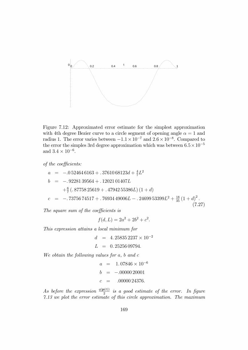
t 10.80.60.40.200

Figure 7.12: Approximated error estimate for the simplest approximationwith 4th degree Bezier curve to a circle segment of opening angle α = 1 andradius 1. The error varies between −1.1×10−7 and 2.6×10−8. Compared tothe error the simples 3rd degree approximation which was between 6.5×10−5and 3.4× 10−6.

of the coefficients:

a = −.0 52464 6163 + . 37610 68123d+ 47L2

b = −. 92281 39564 + . 12021 01407L

+67(. 87758 25619 + . 47942 55386L) (1 + d)

c = −. 73756 74517 + . 76934 49006L− . 24699 53399L2 + 1835(1 + d)2 .

(7.27)The square sum of the coefficients is

f(d, L) = 2a2 + 2b2 + c2.

This expression attains a local minimum for

d = 4. 25835 2237× 10−2

L = 0. 25256 09794.

We obtain the following values for a, b and c

a = 1. 07846× 10−6

b = −.00000 20001c = .00000 24376.

As before the expression q(p(t))2

is a good estimate of the error. In figure7.13 we plot the error estimate of this circle approximation. The maximum

169

t 10.80.60.40.20

0

0

Figure 7.13: The error in the circle approximation error resulting from findingan approximate minimum of the square sum of the coefficients of q(p(t)) foropening angle α = 1.0. The maximal error is less than 6.6× 10−8. Which isapproximately half of the error the simplest circle approximation.

value of the error is approximately half of the error for the simplest O(α8)approximation method.

As in Section 7.2 we can produce a wide variety of circle approximationswith the 4th degree Bezier curve. E.g. an equioscillating circle approximationis assumed to exist. The error estimate q(p(t))

2of this has the shape of the

8th degree Bezier function equioscillating function defined by the vertices

(0, 0, 1,−u, v,−u, 1, 0, 0),

where u and v can be shown to be by lengthy calculations to be

v = (28 + 20u+ 9u2 − 3√3(2 + u)2)/10

u = 2(√3− 6)/9 + 2

√2(K

3/42 +K

1/23 )/(9K

1/61 K

1/42 )

K3 = 54√2(1 +

√3)K

1/21 + (5 + 32

√3 + (16 + 14

√3−K

1/31 )K

1/31 )K

1/22

K2 = −5− 32√3 + (8 + 7

√3 +K

1/31 )K

1/31

K1 = −172 + 3√3(−55 + 54

q2(1 +

√3)).

A numeric approximation to u and v with 50 digits in Maple gives

u = 3.3975842919587644617862134245043548479555002743432

v = 4.845962784049467271367758780114917624986467464035.

170

t 10.80.60.40.20

0

0

0

0

Figure 7.14: The error in the degree four circle approximation with equioscil-lation of q(p(t)) for opening angle α = 1.0. The maximal error is less than1.8× 10−8. This is approximately 1

6of the error of the simplest degree four

circle approximation, and 13of the circle approximation with the minimum

square sum of the coefficients of q(p(t)).

Example 112 (Fourth Degree Equioscillating Circle Approximation.)We now make an approximation to the equioscillating error function by usinga, b and c as defined in (7.27) with ten digit accuracy. We then solve theequation

a u = −ba v = c

to enforce the equioscillation. The approximative solution we find is

L = 0. 25255 0802

d = 4. 25900 3677× 10−2,

which gives the following values

a = 5. 9101× 10−7

b = −.00000 20073c = 0.00000 28641.

Then in figure 7.14 we show the plot of error estimate q(p(t))2. Note that the

error is less than 13of the error for the approximation with minimum square

sum of the coefficients.

171

Bibliography

[APS:87] Dokken, T., Reference Manual, APS B-spline Libraryversion 3.3., ISBN-7267-930-2, Senter for Industriforskn-ing, Oslo, Norway, (1987).

[Bajaj:93] Bajaj, C., The Emergence of Algebraic Curves and Sur-faces in Geometric Design, in Directions in GeometricComputing, Information Geometers, (1993),1-28.

[Oslo-algorithm] Cohen, E., T. Lyche and R. Riesenfeld, Discrete B-Splines and Subdivision Techniques in Computer-AidedGeometric Design and Computer Graphics, ComputerGraphics and Image Processing, 14(1980), 87-111.

[Chionh:92] Chionh, E.W. and R. N. Goldmann, Using multivariateresultants to find the implicit equation of a rational sur-face, The Visual Computer 8(1992), 171-180.

[Cox:72] Cox, M. G., The numerical evaluation of B-splines, J.Inst. Math, Appl., 10(1972), 134-149.

[Cox:92,Cox:97] Cox, D., Little, J. and O’Shea, D., Ideals, Varieties andAlgorithms, Springer-Verlag, New York, (1992) & (1997).

[Cox:98] Cox, D., Little, J. and O’Shea, D., Using AlgebraicGeometry, Springer-Verlag, New York, (1998).

[Cox:99] Cox D., Goldman R. and Zhang M., On the Validityof Implicitization by Moving Quadrics for Rational Sur-faces with No Base Points, J. Symbolic Computation 11(1999).

[de Boor:73] de Boor, C., The Quasi-Interpolant as a Tool in El-ementary Polynomial Spline Theory, in ApproximationTheory, G.G. Lorenz (ed), Academic Press, New York,(1973), 269-276.

172

[de Boor:78] de Boor, C., A practical Guide to Splines, Springer-Verlag, (1978).

[de Boor:87-1] de Boor, C., B-form basics, in Geometric Modeling: Al-gorithms and New Trends, G. Farin (ed), SIAM, (1987),131-148.

[de Boor:87-2] de Boor, C., K. Höllig and M. Sabin. High accuracy geo-metric Hermite interpolation, CAGD 4(1987), 269-278.

[Degen:92] Degen, W. L. F., Best Approximation of parametriccurves by splines, in Mathematical Methods in ComputerAided Geometric Design II, T. Lyche and L.L. Schu-maker(eds) Academic Press, Boston, (1992), 171—184.

[do Carmo:92] do Carmo, M. P., Riemannian Geometry, Birkhäuser,Boston·Basel·Berlin, (1992).

[Dokken:85] Dokken, T., Finding Intersections of B-spline repre-sented geometries using recursive subdivision techniques,CAGD 2(1985), 189-195.

[Dokken:89] Dokken, T., V. Skytt and A-M. Ytrehus, Recursive Sub-division and Iteration in Intersections and Related Prob-lems, in Computer Aided Geometric Design, T. Lycheand L.L. Schumaker(eds), Academic Press, (1989), 207-214.

[Dokken:90] Dokken, T., M. Dæhlen, T. Lyche and K. Mørken, Goodapproximation of circles by curvature-continuous Beziercurves, CAGD, 7(1990), 33-41.

[Dokken:97] Dokken, T., Aspects of Algorithms for Manifold Inter-section, in Numerical Methods and Software Tools in In-dustrial Mathematics, M. Dæhlen, and A. Tveito (eds),to appear.

[Farin:92] Farin G., Curves and Surfaces for Computer Aided Geo-metric Design, Academic Press Inc, San Diego (1992).

[Farin:86] Farin, G., Triangular Bernstein-Bezier patches, CAGD3(1986), 83-128.

173

[Fuggeli:93] Fugelli, P., Knot insertion for B-splines - Evaluation ofnew and established algorithms, Master Thesis (in Nor-wegian), University of Oslo, Norway, (1993).

[Farouki:87] Farouki, R. T. and V. T. Rajan, On the numerical con-dition of polynomials in Bernstein from, CAGD 4(1987),191-216.

[Farouki:88] Farouki, R. T. and V. T. Rajan, Algorithms for polyno-mials in Bernstein form, CAGD 5(1988), 1-26.

[Floater:95-1] Floater, M. S., High-order approximation of conic sec-tions by quadratic splines, CAGD 12(1995), 617-637.

[Floater:95-2] Floater, M. S., Rational Cubic Implicitization, inMathe-matical Methods for Curves and Surfaces, M. Dæhlen, T.Lyche and L. L. Schumaker (eds.), Vanderbilt UniversityPress (1995), 151-159.

[Floater:96] Floater, M. S., An analysis of cubic approximationschemes for conic sections, Advances in ComputationalMathematics 5(1996), 361-379.

[Floater:97] Floater, M. S., An O(h2n) Hermite approximation forconic sections, CAGD 14(97), 135-151.

[Golub & Loan:83] Golub, G. H. and C. F. van Loan, Matrix Computations,North Oxford Academic, (1983).

[GPM-16:80] Hasund, K., T. Dokken, S. Ulfsby, GPM Report No 16,System Specifications, Sculptured Surfaces, Sentralinsti-tutt for industriell forskning, Oslo, Norway, (1980).

[GPM-26:83] Dokken T. et. al, Reference Manual, B-spline Library,Version 1.0, Sentralinstitutt for industriell forskning,Oslo, Norway, (1983).

[Hoschek:93] Hoschek J. and D. Lasser, Fundamentals of computeraided geometric design, A K Peters, (1993).

[Hohmeyer:92] Hohmeyer, M. E., Robust and Efficient Surface Intersec-tion for Solid Modelling, Report No. UCB/CSD 92/681,Computer Science Division, University of California,(1992).

174

[Hoffmann:90] Hoffmann, C.M., “Algebraic and Numerical Techniquesfor Offsets and Blends,” in Computations of Curves andSurfaces, S. Micchelli, M. Gasea and W. Dahmen (eds),Kluwer Academic, Boston, (1990), 499-528.

[Hoffmann:89] Hoffmann, C. M., Geometric & Solid Modelling, An In-troduction, Morgan Kaufmann Publishers, Inc, San Ma-teo, California, (1989).

[Hoffmann:93] Hoffmann, C. M., Implicit Curves and Surfaces inCAGD. IEEE Computer Graphics & Applications,13(1993), 79-88.

[Hollig:88] Höllig, K., Algorithms for rational spline curves. ARO-Report 88-1, (1988) 287-300.

[Höllig:95] Höllig, K. and J. Koch, Geometric Hermite Interpolation,CAGD 12(1995), 567-580.

[Höllig:96] Höllig, K. and J. Koch, Geometric Hermite Interpolationwith maximal order and smoothness, CAGD 13 (1996),681-695.

[Kriezes:90-1] Kriezis, G. A., Algorithms for Rational Spline SurfaceIntersection, Ph. D. Thesis, Massachusetts Institute ofTechnology, Boston, (1990).

[Kriezes:90-2] Kriezis, G. A. and N. M. Patrakalakis. Rational polyno-mial surface intersection, Technical Report 90-9, MITOcean Engineering Design Laboratory, Boston, June(1990).

[Kriezes:91] Kriezis, G. A. and N. M. Patrakalakis. Rational poly-nomial surface intersections, in Proceedings of the17 ASME Design Automation Conference, September(1991).

[Krishnan:96] Krishnan, S. and D. Manocha, An Efficient Surface Inter-section Algorithm based on the Lower Dimensional For-mulation, ACM Trans. on Graphics 16(1997), 74—106.

[Lyche:94] Lyche, T. and K. Mørken, A Metric for Parametric Ap-proximation, in Curves and Surfaces in Geometric De-sign, P-J. Laurent, A. Le Méhauté and L.L. Schumaker

175

(eds), A.K. Peter, Wellesley, Massachusetts, (1994), 311-318.

[Mountaudouin:89] Mountaudouin, Y. D., Cross product of cones of revolu-tion. CAD, 21(6)(1989).

[Moerken:91-1] Mørken, K., Some identities for products and degree rais-ing of splines, Constr. Approx 7 (1991), 195-208.

[Moerken:91-2] Mørken, K., Best Approximation of Circle Segments byQuadric Bézier curves, in Curves and Surfaces, P-J. Lau-rent, A. Le Méhauté and L.L. Schumaker (eds), Acad-emic Press, Boston, (1991), 331-336.

[Numres:88] Press, Flannery, Teukolsky and Vetterling, NumericalRecipes in C, Cambridge University Press, Cambridge,(1988), 60-71.

[Sederberg:83] Sederberg, T. W., Implicit and Parametric Curves andsurfaces for Computer Aided Geometric Design, Ph.D.Thesis, Purdue University, (1983).

[Sederberg:84-1] Sederberg, T. W., D. C. Anderson and R. N. Goldman,Implicit Representation of parametric curves and sur-faces, Computer Vision, Graphics and Image Processing28(1984), 72-84.

[Sederberg:84-2] Sederberg, T. W., Planar Piecewise Algebraic Curves.CAGD (1984), 241-255.

[Sederberg:88] Sederberg, T. W. and R. J.. Meyers, Loop detection insurface patch intersections. CAGD 5(1988), 161-171.

[Sederberg:89-1] Sederberg, T.W., H. N. Christiansen and S. Katz. An im-proved test for closed loops in surface intersection, CAD21(1989), 505-508.

[Sederberg:89-2] Sederberg, T. W., An algorithm for algebraic curve in-tersection, CAD 21(1989), 547-554.

[Sederberg:89-3] Sederberg, T. W., J. Zhao and A.K. Zundel, Approxima-tive parametrization of algebraic curves, in Theory andPractice of Geometric Modeling W. Strasser and H.-P.Seidel (eds), Springer, Berlin, (1989), 33-54.

176

[Sederberg:89-4] Sederberg, T. W., S.R. White and A.K. Zundel, Fatarcs: A bounding region with cubic convergence, CAGD6(1989), 205-218.

[Sederberg:90] Sederberg, T. W., Techniques for cubic algebraic Sur-faces, IEEE CG & A July 1990, 14-25.

[Sederberg:91] Sederberg, T. W., and Tomoyuki Nishita, Geomet-ric Hermite approximation of surface patch intersectioncurves, Computer Aided Geometric Design 8(1991), 97-114.

[Sederberg:95] Sederberg, T. W., and F. Chen, Implicitization usingmoving curves and surfaces, Computer Graphics AnnualConference Series (1995), 301—308.

[Sederberg:96] Sederberg, T.W. and A.K. Zundel, Pyramides thatbound surface patches. CVGIP: Graphics Models andImage Processing, (1996), 75-81.

[Sederberg:97] Sederberg, T. W., Goldman R.N. and Du H., Implicitiza-tion Rational Curves by the Method of Moving AlgebraicCurves, J. Symbolic Computation, 23(1997), 153-175.

[Sederberg:99] Sederberg, T.W., Zheng J., Klimaszewski K. and DokkenT, Approximate Implicitization Using Monoid Curvesand Surfaces, Graphical Models and Image Processing61, 177-198 (1999).

[Seidel:92] Seidel, H.P., Presenting Piecewise Polynomials as LinearCombinations of Multivariate Splines, in MathematicalMethods in Computer Aided Geometric Design II, T. Ly-che and L. L. Schumaker(eds.) Academic Press, Boston,(1992), 559-566.

[SISL:94] SISL - The SINTEF Spline Library, version 4.0, SINTEF,Oslo, Norway, December 1994.

[Stewart:73] Stewart, G. W., Introduction to Matrix Computations,Academic Press, New York & London, (1973).

[Sinha:85] Sinha, P., E. Klassen and K.K. Wang, Exploiting topo-logical and geometric properties for selective subdivision.In ACM Symposium on Computational Geometry, ACMPress, (1985), 39-45.

177

[Spivak:79] Spivak, M., A comprehensive Introduction to DIFFER-ENTIAL GEOMETRY, volume 1, second edition, Pub-lish or Perish Inc, (1979).

[IVF:94] Wandebäck, F. and H. Johansson, Kvalitetssäkring avCAD-geometri. IVF-RAPPORT 94028, Institutet förVerkstadsteknisk forskning, Göteborg,Sweden, (1994).

[Schaback:92] Schaback, R., Rational Geometric Curve Interpolation,in Mathematical Methods in Computer Aided GeometricDesign II, T. Lyche and L. L. Schumaker (eds), AcademicPress, Boston, (1992), 517-535.

[Weiler:86] Weiler, K. J., Topological Structures for Geometric Mod-elling, Ph.D. Thesis, Renesselaer Polytechnic Institute,Report No. TR-86032, Troy, New York, (1986).

[Zundel:94] Zundel, A.K, Surface-Surface Intersection: Loop De-struction Using Bézier Clipping and Pyramidal Bounds.Thesis for Doctor of Philosophy, Brigham Young Univer-sity, (1994).

[Zundel:96] Zundel, A.K and T. W. Sederberg, Surface IntersectionLoop Destruction, Technical report from Brigham YoungUniversity, Department of Computer Science (1996).

178

Appendix A

PosProd Basis Functions

In this appendix we look into the most used basis functions in CAD/CAM-systems and show that these are Pos Prod Basis functions. In AppendixA.1 we address tensor product B-splines. Then in respectively appendix A.2and A.3 we address Bernstein Bases defined over a simplex and the tensorproduct Bernstein Bases.

A.1 Tensor Product B-splines

The B-spline basis functions are piecewise polynomials of degree n = k − 1defined over a knot vector t1, . . . , tN+k where ti+k > ti and ti+1 ≥ ti andsatisfy

NXi=1

Bi,k(t) = 1

Bi,k(t) > 0, ti < t < ti+k i = 1, . . . , N (A.1)

Bi,k(t) ≥ 0, tk ≤ t ≤ tN+1.

From the total knot sequence t1, . . . , tN+k we take the smaller sequencetk, . . . , tN+1, if ti = . . . = ti+r−1 we say that r is the multiplicity of theknot value ti. A knot vector where all knots have multiplicity equal to thepolynomial order k is called a Bernstein knot vector.Condition 1. in definition 24 on page 46 is satisfied by (A.1). By theorem

3.1 in [Moerken:91-1] condition 2. in definition 24 is satisfied. Thus, the B-spline basis is a Pos Prod Basis. In addition the theorem in [Moerken:91-1]can be used as the basis for a PosProd Algorithm for B-splines.

179

Basis functions built by tensor products of B-spline basis functions

Bi,n(s) =

gYl=1

Bip,(np+1)(sp)

also satisfy the conditions 1. and 2. in definition 24, because we can applythe results of the univariate case to each variable separately.Thus, all manifolds defined by NURBS with positive weights are R-

positive manifolds. The most used of these are:

• 2D NURBS curves with positive weights.

• 3D NURBS curves with positive weights.

• 3D NURBS surfaces with positive weights.

A.2 Bernstein Bases over Simplices

Bernstein basis functions built over a simplex S

S = β1q1 + . . .+ βg+1qg+1 | β1 + . . .+ βg+1 = 1, 0 ≤ βi

with corners q1, . . . ,qg+1, in IRg can be defined by barycentric coordinates(β1(s), . . . , βg+1(s)) that satisfy

µq1 . . . qi−1 qi qi+1 . . . qg+11 . . . 1 1 1 . . . 1

¶⎛⎜⎝ β1...

βg+1

⎞⎟⎠ =

µs1

¶.

Here β1(s) + . . . + βg+1(s) = 1 is just the last equation. For references see[Sederberg:84-2], [Farin:86] and [de Boor:87-1]. When s ∈ S, s has to be aconvex combination of the corners of the simplex. By Cramers rule we get

βi(s) =

¯q1 . . . qi−1 s qi+1 . . . qg+11 . . . 1 1 1 . . . 1

¯¯q1 . . . qg+11 . . . 1

¯ , i = 1, . . . , g + 1.

Bernstein basis functions built over a simplex S are defined by

Bi,n(s) = n!

g+1Yl=1

(βl(s))il

il!=

n!

i1! . . . ig+1!(β1(s))

i1 . . .¡βg+1(s)

¢ig+1 . (A.2)

180

Here we have used n instead of n since we have the same maximal polynomialdegree in all variables. The index set I is defined by

I = (i1, . . . , ig+1) | i1 + . . .+ ig+1 = n, il ∈ IN0, l = 1, . . . , g + 1.

The number of multi indices in I are N =

µn+ g

g

¶, which can be proved by

recursion on n+ g.

Lemma 113 The Bernstein basis functions built over a simplex defined asin equation (A.2) satisfyX

i∈IBi,n(s) = 1 (A.3)

Bi,n(s) ≥ 0, i ∈ I, s ∈ Ω.

Proof. See [Farin:86] or [de Boor:87-1].

Lemma 114 Let the functions p(s) and q(s) in g-variables be represented byBernstein basis functions over a simplex.

p(s) =Xi∈Ip

piBi,np(s)

q(s) =Xj∈Iq

qjBj,nq(s).

Then the product of p(s)q(s) can be expressed as

p(s)q(s) =Xi∈Ip

Xj∈Iq

piqjBi,np(s)Bj,nq(s)

=Xk∈Ipq

gkBk,np+nq(s),

where k =(k1 . . . , kg+1), j = (j1, . . . , jg+1) and i = (i1, . . . , ig+1) with

gk =np!nq!

(np + nq)!

min(kl,np)Xil=max(0,kl−nq)

l=1,...,g+1

g+1Yl=1

µklil

¶pi qk−i. (A.4)

If the coefficients satisfy

pi ≥ 0, i ∈Ipqj ≥ 0, j ∈Iq,

thengk ≥ 0, k ∈Ipq.

181

Proof. See [Farin:86] or [de Boor:87-1].Equation (A.4) is a PosProd Algorithm since, as stated in theorem 29, gk

are calculated as a convex combination of all pi qj.Thus manifolds described by simplical rational Bernstein Bases with pos-

itive weights are R-positive manifolds. The most used of these are:

• 2D Bezier curves with positive weights. (This is a special instance of2D NURBS curves)

• 3D Bezier curves with positive weights. (This is a special instance of3D NURBS curves)

• 3D rational triangular Bezier surfaces with positive weights.

3D rational tetrahedral Bezier volumes with positive weights are not in-cluded. This as the definition of R-positive manifolds requires that the di-mension of the manifold is lower than the dimension of the space in whichthe manifold lies.

A.3 Tensor Product Bernstein Basis

The tensor product Bernstein basis is a special instance of the B-spline bases.Knot insertion can bring a B—spline represented function to a Bernstein knotvector and thus to the representation as a set of Bernstein basis representedfunctions. The overhead of the extra knots in a Bernstein knot vector is not sosevere when products of functions are calculated as it is in the representationof the original functions. Since the algorithms for Bernstein basis representedobjects are simpler than with B-spline basis represented objects, we go intosome detail here, although the properties are already shown in Appendix A.1on tensor product B-splines.

Example 115 Let pi(s), i = 1, . . . ,m be univariate B-spline representedfunctions with N coefficients of order k with k-tupple knots at the ends andsingle internal knots. The piecewise polynomial functions consist of N−k+1polynomial segments. The same function represented with a Bernstein knotvector requires (N − k + 1)k coefficients. The overhead compared to the B-spline representation is

(N − k + 1)k −N.

When we make products of m such functions the overhead will not growwhile the total storage for the Bernstein knot vector representation will be(N − k + 1)((k − 1)m + 1). Now making the quotient between the overhead

182

and what is needed for storage of the product of m functions with a Bernsteinknot vector we get

(N − k + 1)k −N

(N − k + 1)((k − 1)m+ 1)=

k − NN−k+1

(k − 1)m+ 1≤ k − 1(k − 1)m+ 1

<1

m.

Thus, as the number of functions being multiplied increase, the relative effectof the overhead is small compared to the total number of coefficients. Whenthe functions are at least C1 relative simple techniques can be used to storethe functions with a reduced Bernstein knot vector with k−2 multiple internalknots, thus bringing the overhead further down.

An algorithm for calculating the coefficients of the product of two bi-variate Bernstein basis represented functions is given in [Farouki:88]. Thisalgorithm is generalized in the following lemma.

Lemma 116 Let the functions p(s) and q(s) in g-variables defined over theunit cube in IRg be represented in a tensor product Bernstein basis

p(s) =

nlXil=0

l=1,...,g

pi1,...,ig

gYr=1

Bnrir (sr)

q(s) =

mlXil=0

l=1,...,g

qi1,...,ig

gYr=1

Bmrir(sr)).

Here

Bmi (u) =

µmi

¶ui(1− u)(m−i),

andnlXil=0

l=1,...,g

=n1Xi1=0

. . .

ngXig=0

.

Then the product of p(s) and q(s) can be expressed as

p(s)q(s) =

nlXil=0

l=1,...,g

mkXjk=0

k=1,...,g

pi1,...,igqj1,...,jg

gYr=1

¡Bnrir (sr)B

mrjr (sr)

¢

=

nl+mlXil=0

l=1,...,g

gi1,...,ig

gYr=1

Bnr+mrir

(sr),

183

where

gi1...,ig =

min(il,nl)Xpl=max(0,il−ml)

l=1,...,g

cp1,...,pgdi1−p1,...,ig−pg

gYr=1

∙µnrpr

¶µmr

ir − pr

¶¸gY

r=1

µnr +mr

ir

¶ . (A.5)

Proof. See [de Boor:87-1].The product algorithm in (A.5) is a PosProd Product Algorithms since,

as stated in remark 29, the coefficients g(s) are convex combinations of thecoefficients of p(s) and q(s).

184

Appendix B

Reformulation of GeometricInterrogations to ManifoldIntersections

In the main part of the thesis we have concentrated the discussions on prob-lems related to the intersection of smooth bounded manifolds in IRl. Weaddress in this appendix a number of geometric interrogations problems thatcan be reformulated to intersection of manifolds. Many of the reformulationsaddressed are implemented in the SISL library [SISL:94]. This appendix isbased on the work in [Dokken:85].The intersection algorithms in SISL - SINTEF Spline Library are based

on an intersection kernel that address the intersection of two manifolds ofpossibly different dimensions. The manifolds being intersected in SISL are:

• 0-manifolds (points) in IR2 and IR3.

• NURBS represented 1-manifolds (curves) in IR2 and IR3.

• NURBS represented 2-manifolds (surfaces) in IR3.A special feature in SISL is the possibility to find common zeroes of

two NURBS represented functions defined on the same 1-dimensional or 2-dimensional compact domain. The functions are expanded to 1-manifolds inIR2 or 2-manifolds in IR3 when properties of manifold intersections have tobe used. This feature has enabled the implementation of a wide range ofintersection related functions in SISL.We address in this appendix such functionality integrated into SISL, but

also look at possibilities emerging with an intersection kernel handling higherdimensional manifolds than 2-manifolds and higher dimensional real spacesthan IR3. The discussion is structured as follows:

185

• In Appendix B.1 we address:

— The intersection of algebraic curves and parametric curves in IR2.

— The intersection of algebraic surfaces and parametric curves inIR3.

— The intersection of algebraic surfaces and parametric surfaces inIR3.

• Generating silhouette curves of different kinds is addressed in AppendixB.2.

• Projection of a manifold onto another manifold is addressed in Appen-dix B.3.

• Finding extremal points on a curve or surface with respect to a directionis in SISL converted to searching for extremal values of a functiondefined over the parameter domain of respectively a curve or a surface.The same is the case for finding the points on a curve or a surfacebeing closest to a given point, or the points on two curves being closest.Aspects of searching for extremal values of such functions are addressedin Appendix B.4.

B.1 Intersection of Parametric RepresentedManifolds and Hypersurfaces

In Section 2.5.5 we showed that the dimensionality of an intersection problemcan be reduced by combining parametric described manifolds and hypersur-faces. Many of the interrogation problems in CAD-systems can be formulatedin such a way. In SISL the following intersections have been implemented byusing such combinations:

• Intersection of a NURBS curve and a straight line in IR2.

• Intersection of a NURBS curve and a circle in IR2.

• The intersection of a general second degree algebraic curve and a NURBScurve.

• The intersection of a NURBS surface and a plane in IR3.

• The intersection of a NURBS surface and a sphere in IR3.

186

• The intersection of a NURBS curve and a torus in IR3.

• The intersection of a general second degree algebraic surface and aNURBS surface in IR3.

• The intersection of a straight line and a NURBS surface.

• The intersection of a circle and a NURBS surface.

• The intersection of a torus and a NURBS surface.

The simplest extensions to higher dimensional problems is the intersectionof 1- and 2-manifolds with hypersurfaces. This results in finding zeroes offunctions in 1 or 2 variables and can for NURBS represented geometriesbe addressed by SISL. However, the intersection of manifolds of dimensiong > 2 and hypersurface requires an intersection kernel handling manifolds ofdimension g > 2.The main challenge of combining algebraic and parametric representa-

tions is to ensure that the functions resulting from the combination haveminimal rounding errors. In Section 4.1 we addressed the problem of combin-ing R-positive manifolds with hypersurfaces, and showed in Section 4.2 thatthe use of PosProd Algorithms resulted in a controlled growth of the relativerounding errors. An alternative to PosProd Algorithms is to use methodsthat reproduce polynomial behavior. One such method is B-spline interpo-lation. However, as the algebraic degree is growing, the condition number ofthe coefficient matrix of the B-spline interpolation increases. Although thecondition number reflects a worst case, practical experience has shown thatthe use of PosProd Algorithms is to be preferred over interpolation methods.

B.2 Finding Silhouette Curves in IR3

In SISL three different silhouette calculations have been implemented byreformulation approach:

• Parallel silhouettes.

• Perspective silhouettes.

• Circular silhouettes.

To give a complete silhouette calculation we have to consider both:

187

• The zeroes of the function representing the reformulated silhouetteproblem.

• Edges and break lines.

In all of the silhouette calculations the normal vector of the surface playa central role. Thus, we address the normal vector in Section B.2.1.

B.2.1 The normal vector

When a surface p(s1, s2) of degree (n1, n2) is nonrational the normal is as weknow

n(s1, s2) =∂p(s1, s2)

∂s1× ∂p(s1, s2)

∂s2.

Resulting in a polynomial degree for the normal of (2n1 − 1, 2n2 − 1).In case p(s1, s2) is rational, the degrees of the numerator of n(s1, s2) are

(4n1 − 1,4n2 − 1), and of the denominator (4n1, 4n2). However, the denomi-nator h(s, t) is a factor in both the numerator and denominator of n(s1, s2).Thus, cancelling this we get degrees (3n1 − 1,3n2 − 1) in the numerator and(3n1, 3n2) of the denominator.To control the propagation of the rounding error, PosProd Algorithms

can be used for making the normal vector.

B.2.2 Parallel Projection Silhouette in IR3

The silhouettes of the parallel projection in a direction e are points where

n(s1, s2) · e = 0.

The polynomial order is related to the polynomial order of n(s1, s2) which isgiven above.

B.2.3 Perspective Silhouette in IR3

The silhouette curves resulting from a perspective projection with respect toa point p0 have to satisfy

n(s1, s2) · (p(s1, s2)− p0) = 0.

The polynomial degrees of the numerator is (4n1 − 1,4n2 − 1) and of thedenominator (4n1, 4n2). If the surface is nonrational the polynomial degreeis (3n1 − 1, 3n2 − 1).

188

B.2.4 Circular Silhouette in IR3

Let p(s1, s2) be a point on a surface and n(s1, s2) be the normal in p(s1, s2).Let q be a point on an axis and b be the direction vector of the axis. Thecircular silhouette curves are defined by

n(s1, s2)× (p(s1, s2)− q) · b = 0.

The polynomial degrees of the numerator is (4n1 − 1,4n2 − 1) and of thedenominator (4n1, 4n2). If the surface is nonrational, the polynomial degreeis (3n1 − 1, 3n2 − 1).

B.3 Projection of a Manifold onto anotherManifold

These functions are not implemented in SISL but can be of use in geometricmodeling systems. Two problems are addressed:

• Normal projection of a manifold onto another manifold.

• Parallel projection of a manifold onto another manifold.

B.3.1 Normal Projection

The normal projection of a g1-manifold p(s) onto a g2-manifold q(t) can beformulated as

(q(t)− p(s)) · ∂q(t)∂ti

= 0, i = 1, . . . , g2,

resulting in g2 functions in g1 + g2 variables.

Remark 26 For g1 = g2 = 1 we have the normal projection of a curve ontoanother curve.

Remark 27 For g1 = 1 and g2 = 2 then we have the normal projection of aparametric curve onto a parametric surface.

Remark 28 For g1 = 2 and g2 = 1 we have an the intersection of the normalplane of a parametric curve with a parametric surface.

189

B.3.2 Parallel Projection

The parallel projection of a parametric g1-manifold p(s) onto a parametricg2-manifold q(t) in IRl satisfies

(q(t)− p(s)) · nj = 0, j = 1, . . . , l − 1.

Here nj, j = 1, . . . , l−1 are linearly independent vectors normal to projectiondirection e. The result is l − 1 functions in g1 + g2 variables.

Remark 29 If p(s) and q(t) both are in IR3, g1 = 1 and g2 = 2, then wehave the parallel projection of a curve onto a surface. Interchanging g1 andg2 does not change the geometric interpretation.

B.4 Reformulation to extremal value prob-lems.

Many problems can be reformulated to finding the extremal value of a func-tion defined over the parameter domain of a manifold or of the tensor productof the parameter domains of two manifolds.Let Ω ∈ IRg, be a bounded set over which we define a continuous function

f : Ω→ IR that is piecewise smooth, and where the smooth pieces are limitedby a set Ωb that can be decomposed into (g − 1)-manifolds contained in Ω.Ωb is thus also containing the boundary of Ω. To find the maximal values ofthe function the following approaches can be used:

• Use a tradition analyses of extremal values based on (partial) deriva-tives and analysis of the behavior of the function along the manifoldsdescribing the piecewise smooth structure Ωb.

• Apply a direct search for the extremal values by combining iterationand subdivision techniques.

In SISL the last approach is employed for efficiency reasons. This tomake a generic tool for finding extremal values of NURBS based functions inone or two variables. However, this approach is also too slow when repeateduse of the extremal value calculation is necessary. In these cases an itera-tion using as start point the result of the previous search for an extremalvalue, can be used. In these cases it is often too expensive to evaluate thefunction f for each search, and the iteration is performed on the originalgeometries. However, the iterations can fail and fallback strategies have tobe implemented.

190

In SISL the following problems are addressed using the search for extremalvalues:

• Find the point closest to a given point q on a NURBS represented curvep(s). The function searched for extremal values is

f(s) = (p(s)− q) · (p(s)− q).

This is the same as the function for the intersection of a circle or sphereof radius 0 and a curve.

• Find the point closest to a given point q on a NURBS representedsurface p(s). The function searched for extremal values is

f(s, t) = (p(s, t)− q) · (p(s, t)− q).

This is the same as the function for the intersection of a circle or sphereof radius 0 and a surface.

• Find the closest points between two NURBS represented curves p(s)and q(t). The function searched for extremal values is

f(s, t) = (p(s)− q(t)) · (p(s)− q(t)).

• Find the extremal point(s) on a NURBS represented curve p(s) in thedirection d. The function searched for extremal values is

f(s) = p(s) · d.

• Find the extremal point(s) on a NURBS represented surface p(s, t) inthe direction d. The function searched for extremal values is

f(s, t) = p(s, t) · d.

191