aspects of quantum gravity phenomenology soumen …
TRANSCRIPT
.
ASPECTS OF QUANTUM GRAVITY PHENOMENOLOGY
SOUMEN DEBBachelor of Science, University of Calcutta, 2008
Master of Science, Indian Institute of Technology Bombay, 2010
A ThesisSubmitted to the School of Graduate Studies
of the University of Lethbridgein Partial Fulfilment of the
Requirements for the Degree
MASTER OF SCIENCE
Department of Physics and AstronomyUniversity of Lethbridge
LETHBRIDGE, ALBERTA, CANADA
c© Soumen Deb, 2015

ASPECTS OF QUANTUM GRAVITY PHENOMENOLOGY
SOUMEN DEB
Date of Defense: January 14, 2015
Dr. Saurya Das Professor Ph.D.Supervisor
Dr. Mark Walton Professor Ph.D.Thesis Examination Committee Member
Dr. Kent Peacock Professor Ph.D.Thesis Examination Committee Member
Dr. Locke Spencer Assistant Professor Ph.D.Chair, Thesis Examination Committee
To the bright memory of my father, Dr. Priyaranjan Deb
iii
Abstract
Quantum gravity effects modify the Heisenberg’s uncertainty principle to the
generalized uncertainty principle (GUP). Earlier work showed that the GUP-induced
corrections to the Schrodinger equation, when applied to a non-relativistic particle in
a one-dimensional box, led to the quantization of length. Similarly, corrections to the
Klein-Gordon and the Dirac equations, gave rise to length, area and volume quanti-
zations. These results suggest a fundamental granular structure of space. This thesis
investigates how spacetime curvature and gravity might influence this discreteness of
space. In particular, by adding a weak background gravitational field to the above
three quantum equations, it is shown that quantization of lengths, areas and volumes
continue to hold. Although the nature of this new quantization is quite complex,
under proper limits, it reduces to cases without gravity. These results indicate the
universality of quantum gravity effects.
iv
Acknowledgements
This work was supported by the Natural Sciences and Engineering Research Coun-
cil of Canada (NSERC) and the University of Lethbridge.
I am thankful to my supervisor Dr. Saurya Das for his inspiring guidance, con-
structive criticism, friendly advice and academic as well as non-academic support
throughout the research project. I would like to express my gratitude to my commit-
tee members Dr. Mark Walton and Dr. Kent Peacock for all the valuable suggestions
and comments they provided.
I would also like to thank my family and friends for their help and encouragement.
v
Contents
List of Figures viii
1 Introduction 11.1 Prologue . . . . . . . . . . . . . . . . . . . . . . . . . . . . . . . . . . 11.2 Quantum Gravity Phenomenology . . . . . . . . . . . . . . . . . . . . 4
1.2.1 Why Phenomenology . . . . . . . . . . . . . . . . . . . . . . . 41.2.2 Goals of Quantum Gravity Phenomenology . . . . . . . . . . . 41.2.3 Uncertainties within Quantum Gravity . . . . . . . . . . . . . 6
1.3 Generalized Uncertainty Principle from String Theory: Discreteness ofSpace . . . . . . . . . . . . . . . . . . . . . . . . . . . . . . . . . . . . 6
1.4 Discreteness in Flat Spacetime . . . . . . . . . . . . . . . . . . . . . . 81.4.1 Non-relativistic case . . . . . . . . . . . . . . . . . . . . . . . 81.4.2 Relativistic one-dimensional case . . . . . . . . . . . . . . . . 111.4.3 Relativistic two and three-dimensional cases . . . . . . . . . . 13
2 Discreteness of Space from GUP : Non-relativistic Case 162.1 Discreteness of Space in Presence of Gravity . . . . . . . . . . . . . . 162.2 Solution of Schrodinger Equation with a One-dimensional Linear Po-
tential . . . . . . . . . . . . . . . . . . . . . . . . . . . . . . . . . . . 172.3 GUP-corrected Schrodinger Equation with a One-dimensional Linear
Potential . . . . . . . . . . . . . . . . . . . . . . . . . . . . . . . . . . 222.4 Solution of the GUP-corrected Schrodinger Equation: . . . . . . . . . 22
2.4.1 Perturbative Solutions . . . . . . . . . . . . . . . . . . . . . . 222.4.2 Non-perturbative Solution . . . . . . . . . . . . . . . . . . . . 292.4.3 General Solution . . . . . . . . . . . . . . . . . . . . . . . . . 30
2.5 Boundary Conditions and Length Quantization . . . . . . . . . . . . 32
3 Discreteness of Space from GUP : Relativistic Case 383.1 Klein-Gordon Equation in One dimension . . . . . . . . . . . . . . . 383.2 Dirac Equation . . . . . . . . . . . . . . . . . . . . . . . . . . . . . . 403.3 Solution of Dirac Equation . . . . . . . . . . . . . . . . . . . . . . . . 42
3.3.1 Perturbative solution . . . . . . . . . . . . . . . . . . . . . . . 423.3.2 Non-perturbative solution . . . . . . . . . . . . . . . . . . . . 45
3.4 Boundary Condition and Length Quantization . . . . . . . . . . . . . 453.5 Dirac Equation in Three Dimensions . . . . . . . . . . . . . . . . . . 543.6 Boundary Conditions . . . . . . . . . . . . . . . . . . . . . . . . . . . 56
vi
3.6.1 Case 1 : Length quantization along x axis . . . . . . . . . . . 593.6.2 Case 2 : Length quantization along y and z axes . . . . . . . . 63
4 Conclusions 664.1 Introduction . . . . . . . . . . . . . . . . . . . . . . . . . . . . . . . . 664.2 Summary of the Results . . . . . . . . . . . . . . . . . . . . . . . . . 674.3 Significance of the Results . . . . . . . . . . . . . . . . . . . . . . . . 684.4 Future Directions of Work . . . . . . . . . . . . . . . . . . . . . . . . 69
Bibliography 70
Appendices 73
A Dimensions and Relative Magnitudes 74
B Dimension Check for k and Comparison with α 76
C Derivatives 78C.1 Computation of some useful quantities . . . . . . . . . . . . . . . . . 78C.2 Calculation of derivatives required in sec 2.3.1 . . . . . . . . . . . . . 80
vii
List of Figures
2.1 Airy functions and the zeroes [35] . . . . . . . . . . . . . . . . . . . . . 182.2 H as a function of k (for particles with finite mass and large but finite
Energy) . . . . . . . . . . . . . . . . . . . . . . . . . . . . . . . . . . 212.3 Comparison between L0(solid lines) and L (dotted lines) . . . . . . . 37
viii
Chapter 1
Introduction
1.1 Prologue
Quantum field theory describes the behavior of the fundamental constituent parti-
cles and the fields. General relativity, on the other hand, treats one of the fundamental
forces, gravity as a derived effect of spacetime curvature and explains the large scale
dynamics – from planetary and galactic motions to black hole physics and in general
the evolutionary history of the universe. The two theories are successful in their own
realms, but they are not really mutually compatible. Einstein’s formulation is essen-
tially a deterministic approach. Although it governs the force of gravity, it cannot be
applied the same way to explain gravitational field as the Standard Model does to
the three other fundamental forces of nature, electromagnetic, strong and weak.
Moreover, the presence of mathematical difficulties like singularities in the Feyn-
mann diagrams, renormalization failure etc. [1] [3] in quantum field theory clearly
indicates that a more general formalism is required in order to explain all of the
fundamental forces together.
Hawking Radiation [2] can be considered as an example that, despite being an
area more relevant to the general relativity, explained better with quantum mechanics
in curved spacetime. Rotating and Reissner–Nordstrom black holes, for example, are
expected to emit photons and other particles according to quantum mechanics, the
dynamics of which are well comprehended by general relativity. Although a direct
1
signature is yet to be found, this prediction has also been supported by analog gravity
experiments [14].
Observational evidence like this along with the technical problems with having
two distinct theories suggests a necessity for a successful unification, in other words,
a quantum theory of gravity.
There are a few candidates for a successful quantum gravity theory. String theory,
Loop quantum gravity and Causal set theory are among the most promising ones.
Here is a brief review of these theories.
1. String Theory – this mathematically rigorous theory has a rather simple un-
derlying concept. From the early age of the development of physics, reductionism
has always played the driving force of active research. We expect to find simpler
things as we go deeper. Macroscopic objects to molecules, molecule to atoms, atom
to its constituent particles - reductionism has always worked. Apparently dissimilar
forces boil down to four fundamental forces. Problem occurs beyond this point, when
a unification of these forces was much sought. Standard model required even many
more particles to explain the intrinsic nature of the fundamental forces, and the old
reductionism started to fail. At this point, it appeared string theory came up with a
much-simplified idea of having all fundamental particles either force carriers (bosons)
or that make matter (fermions) as different modes of vibration of the same string. A
string can be a closed loop, which typically represents bosons, or open-ended which
represents fermions [4].
String theory also introduces the concept of D-branes. A brane is a 2-dimensional
membrane or analogous object in lower or higher dimensions. A D-brane or a
Dirichlet-brane is a higher dimensional brane such that the two ends of open-ended
strings are attached to either one single D-brane or two different D-branes [5]. Clearly
this restricts how an open-ended string can vibrate. One of the vibrations can be as-
2
sociated with the gravitational field. In short, string theory appears to solve the
problem of merging gravity with standard model, at least theoretically [6].
Problem with string theory is that the predictions are extremely difficult to test.
For example, String theory predicts for the existence of 9+1 dimensions. This re-
quires postulating six additional unobserved spatial dimensions which is not quite in
agreement with the current experimental evidence.
2. Loop Quantum Gravity(LQG) – the leading alternative to string theory is
loop quantum gravity. This approach uses the principles of general relativity as its
starting point in an effort to quantize both space and time. The basic consideration
of LQG is a granular structure of space which can be viewed as a network of finite
quantized loops of size of Planck length. This network is technically known as a
spin network, the time evolution of which is called a spin foam. These fine loops are
thought to be excited gravitational fields. Unlike string theory, loop quantum gravity
does not head for a theory of everything. It mainly aspires to solve the problem of
quantum gravity, with having the advantage over string theory by not looking for
higher dimensions. A length quantization similar to what we are going to present in
this thesis has been shown in LQG [9].
The biggest flaw in loop quantum gravity is that it is not possible to show that a
smooth spacetime can be extracted out of a quantized space. Also, like string theory
the predictions of LQG are not quite testable yet [7].
3. Causal Set Theory – This approach is based on the assumption that the space-
time is fundamentally discrete and there is a one-to-one map between distinct past
and future events [8]. The consequence of the causal set hypothesis is technically
known as the dynamics of sequential growth. This theory identifies time as a birth
process of consecutive spacetime events, also called the elements of causal set [10].
3
It is debatable that an initial assumption of discreteness of spacetime in any the-
ory might have a conflict with Lorentz invariance. Causal set is able to address to
this problem [11]. Despite being in an early stage of development, causal set theory
successfully predicted the fluctuations in the value of the cosmological constant [10].
Although the dynamics has made progress, a complete theory is yet to come.
1.2 Quantum Gravity Phenomenology
1.2.1 Why Phenomenology
People have been working towards quantum gravity for over 70 years. All quan-
tum gravity theories start with assumptions about the structure of spacetime at scales
that are extremely small, way beyond the current experimental advancement. Be-
cause there is no direct experimental guidance, it is quite natural to try to develop
a correct theory based on indirect criteria of conceptual restrictions. Like any other
active field, what Quantum Gravity Phenomenology ideally needs is a combination of
theory and doable experiments. At the moment, Quantum Gravity Phenomenology
(QGP) can be thought of as a combination of all the studies that might contribute
to direct or indirect observable predictions [12] [13] and analog models [14] support-
ing small and large scale structure of spacetime consistent with string theory or any
other working formalism of quantum gravity. In this thesis we are more interested in
the small scale structure of the spatial dimensions in connection with quantum gravity.
1.2.2 Goals of Quantum Gravity Phenomenology
The first step to identifying the relevant experiments for quantum gravity research
would be the identification of the working scale of this new field. String theory
suggests the characteristic scale where the quantum properties of spacetime become
significant compared to the classical ones is the Planck scale which is Ep ∼ 1028eV
4
or the Planck length `Pl ∼ 10−35 m [15]. This is a difficult part of quantum gravity
phenomenology, i.e., to find ways to detect this very small scale quantum properties
of spacetime. The solution of the quantum gravity problem should also be able to
address the quantum picture of particles in the presence of weak as well as strong
gravity. In other words, we hope quantum gravity phenomenology will helpful towards
grand unification.
The validity of the Equivalence Principle in quantum gravity was first discussed in
the mid 1970s with the famous ”COW” experiment [16]. Experiments and modifica-
tion involving the dynamics of matter in earth’s gravitational field triggered question
on the legitimacy of the Schrodinger equation [17]
[−(
~2
2MI
)∇2 +MGφ(~r)
]ψ(t, ~r) = i~
∂ψ(t, ~r)
∂t, (1.1)
where MI denotes inertial mass and MG denotes gravitational mass, φ(~r) is gravita-
tional potential.
There are no experiments that suggest the inertial and gravitational masses are dif-
ferent on earth. This might indicate a modification in the Schrodinger equation.
String theory suggests a modification in the commutation relation between position
and momenta, which leads to a modified Schrodinger’s equation [32] as well.
One of the basic aims of quantum gravity phenomenologists is to find a way to
test Planck-scale effects of spacetime, which also means providing with boundaries for
the theoretical framework (within which a proper quantum theory of gravity is to be
developed) and information on what is compatible with experimental data. This is
particularly important as the phenomenology is still in its early stage of development.
In this thesis, we will focus on one such experimental limit suggested by quantum
gravity phenomenology which is also consistent with one of the candidate theories,
5
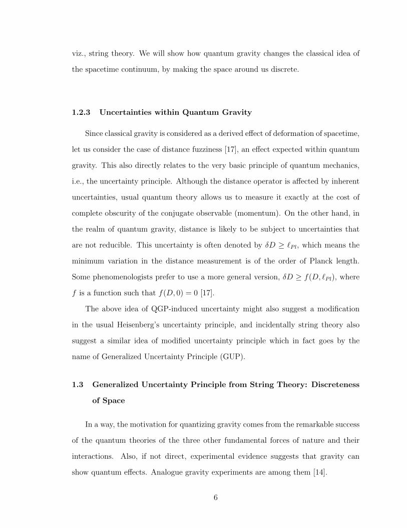
viz., string theory. We will show how quantum gravity changes the classical idea of
the spacetime continuum, by making the space around us discrete.
1.2.3 Uncertainties within Quantum Gravity
Since classical gravity is considered as a derived effect of deformation of spacetime,
let us consider the case of distance fuzziness [17], an effect expected within quantum
gravity. This also directly relates to the very basic principle of quantum mechanics,
i.e., the uncertainty principle. Although the distance operator is affected by inherent
uncertainties, usual quantum theory allows us to measure it exactly at the cost of
complete obscurity of the conjugate observable (momentum). On the other hand, in
the realm of quantum gravity, distance is likely to be subject to uncertainties that
are not reducible. This uncertainty is often denoted by δD ≥ `Pl, which means the
minimum variation in the distance measurement is of the order of Planck length.
Some phenomenologists prefer to use a more general version, δD ≥ f(D, `Pl), where
f is a function such that f(D, 0) = 0 [17].
The above idea of QGP-induced uncertainty might also suggest a modification
in the usual Heisenberg’s uncertainty principle, and incidentally string theory also
suggest a similar idea of modified uncertainty principle which in fact goes by the
name of Generalized Uncertainty Principle (GUP).
1.3 Generalized Uncertainty Principle from String Theory: Discreteness
of Space
In a way, the motivation for quantizing gravity comes from the remarkable success
of the quantum theories of the three other fundamental forces of nature and their
interactions. Also, if not direct, experimental evidence suggests that gravity can
show quantum effects. Analogue gravity experiments are among them [14].
6
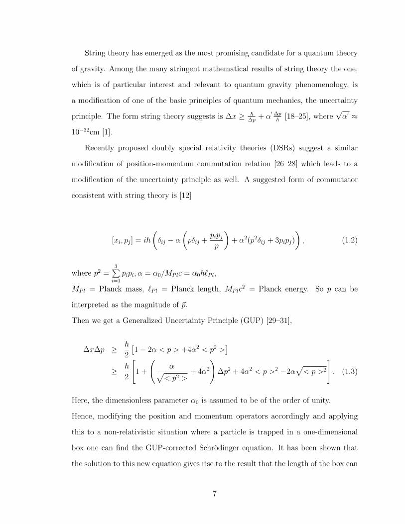
String theory has emerged as the most promising candidate for a quantum theory
of gravity. Among the many stringent mathematical results of string theory the one,
which is of particular interest and relevant to quantum gravity phenomenology, is
a modification of one of the basic principles of quantum mechanics, the uncertainty
principle. The form string theory suggests is ∆x ≥ ~∆p
+ α′ ∆p~ [18–25], where
√α′ ≈
10−32cm [1].
Recently proposed doubly special relativity theories (DSRs) suggest a similar
modification of position-momentum commutation relation [26–28] which leads to a
modification of the uncertainty principle as well. A suggested form of commutator
consistent with string theory is [12]
[xi, pj] = i~(δij − α
(pδij +
pipjp
)+ α2(p2δij + 3pipj)
), (1.2)
where p2 =3∑i=1
pipi, α = α0/MPlc = α0~`Pl,
MPl = Planck mass, `Pl = Planck length, MPlc2 = Planck energy. So p can be
interpreted as the magnitude of ~p.
Then we get a Generalized Uncertainty Principle (GUP) [29–31],
∆x∆p ≥ ~2
[1− 2α < p > +4α2 < p2 >
]≥ ~
2
[1 +
(α√
< p2 >+ 4α2
)∆p2 + 4α2 < p >2 −2α
√< p >2
]. (1.3)
Here, the dimensionless parameter α0 is assumed to be of the order of unity.
Hence, modifying the position and momentum operators accordingly and applying
this to a non-relativistic situation where a particle is trapped in a one-dimensional
box one can find the GUP-corrected Schrodinger equation. It has been shown that
the solution to this new equation gives rise to the result that the length of the box can
7
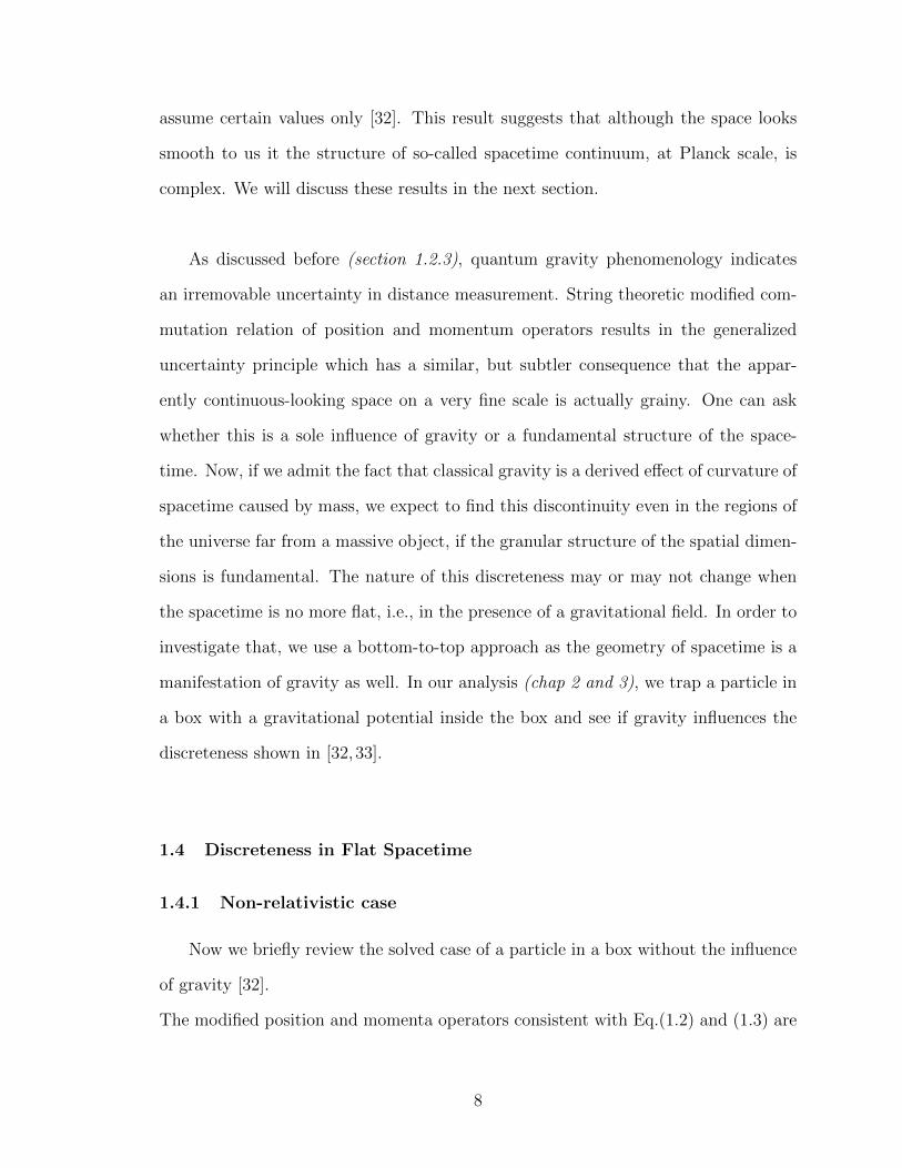
assume certain values only [32]. This result suggests that although the space looks
smooth to us it the structure of so-called spacetime continuum, at Planck scale, is
complex. We will discuss these results in the next section.
As discussed before (section 1.2.3), quantum gravity phenomenology indicates
an irremovable uncertainty in distance measurement. String theoretic modified com-
mutation relation of position and momentum operators results in the generalized
uncertainty principle which has a similar, but subtler consequence that the appar-
ently continuous-looking space on a very fine scale is actually grainy. One can ask
whether this is a sole influence of gravity or a fundamental structure of the space-
time. Now, if we admit the fact that classical gravity is a derived effect of curvature of
spacetime caused by mass, we expect to find this discontinuity even in the regions of
the universe far from a massive object, if the granular structure of the spatial dimen-
sions is fundamental. The nature of this discreteness may or may not change when
the spacetime is no more flat, i.e., in the presence of a gravitational field. In order to
investigate that, we use a bottom-to-top approach as the geometry of spacetime is a
manifestation of gravity as well. In our analysis (chap 2 and 3), we trap a particle in
a box with a gravitational potential inside the box and see if gravity influences the
discreteness shown in [32,33].
1.4 Discreteness in Flat Spacetime
1.4.1 Non-relativistic case
Now we briefly review the solved case of a particle in a box without the influence
of gravity [32].
The modified position and momenta operators consistent with Eq.(1.2) and (1.3) are
8
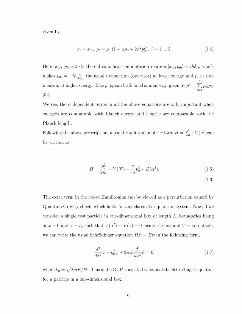
given by,
xi = x0i, pi = p0i(1− αp0 + 2α2p20), i = 1, .., 3. (1.4)
Here, x0i, p0i satisfy the old canonical commutation relation [x0i, p0i] = i~δij, which
makes p0i = −i~ ∂∂x0i
the usual momentum (operator) at lower energy and pi as mo-
mentum at higher energy. Like p, p0 can be defined similar way, given by p20 =
3∑i=1
p0ip0i
[32].
We see, the α dependent terms in all the above equations are only important when
energies are comparable with Planck energy and lengths are comparable with the
Planck length.
Following the above prescription, a usual Hamiltonian of the form H = p2
2m+V (−→r )can
be written as
H =p2
0
2m+ V (−→r )− α
mp3
0 +O(α2). (1.5)
(1.6)
The extra term in the above Hamiltonian can be viewed as a perturbation caused by
Quantum Gravity effects which holds for any classical or quantum system. Now, if we
consider a single test particle in one-dimensional box of length L, boundaries being
at x = 0 and x = L, such that V (−→r ) = V (x) = 0 inside the box and V =∞ outside,
we can write the usual Schrodinger equation Hψ = Eψ in the following form,
d2
dx2ψ + k2
0ψ + 2iα~d3
dx3ψ = 0, (1.7)
where k0 =√
2mE/~2. This is the GUP-corrected version of the Schrodinger equation
for a particle in a one-dimensional box.
9
Let us consider a trial solution of the form ψ = emx. Using this trial solution the
above equation becomes
m2 + k20 + 2iα~m3 = 0 (1.8)
It can be shown that this equation has the solution set to the leading order in α given
by m = ik′0,−ik
′′0 , i/2α~, where k
′0 = k0(1 + k0α~) and k0
′′ = k0(1− k0α~) [32].
The general solution to the GUP-corrected Schrodinger equation in flat spacetime is
thus given by,
ψ = Aeik′0x +Be−ik0
′′x + Ceix/2α~ (1.9)
If we impose the boundary conditions the first two terms, with k′0 = k
′′0 = k0, lead to
the usual quantization of energy. It is to be noted that limα→0 |C| = 0 because the
last term should drop out in the α → 0 limit. This and making A real by absorbing
any phase in ψ, under the boundary condition ψ(0) = 0 yield,
A+B + C = 0. (1.10)
Substituting B from the above in Eq.(1.9),
ψ = 2iA sin(k0) + C[−e−ik0x + eix/2α~
]− α~k2
0x[iCe−ik0x + 2A sin(kx)
](1.11)
The other boundary condition ψ(L) = 0 gives,
2iA sin(k0L) = |C|[e−i(k0L+θC) − ei(L/2α~−θ0)
]+
α~k20L[i|C|e−i(k0L+θC) + 2A sin(k0L)
], (1.12)
10
where C = |C|e−iθC . It is easy to notice that both sides of Eq. (1.12) vanish in the
limit α −→ 0, when k0L = nπ, n is an integer and C = 0 which in turn means when α
is not zero k0L must be equal to nπ plus a small real number ε0, where limα−→0 ε0 = 0.
Also the term containing α|C| on the RHS of Eq.(1.12) has a faster convergence to
zero in the same limit compared to O(α) so it can easily be ignored. Now, collecting
real parts of the rest of the equation and considering sin(nπ + ε0) ≈ 0 we get [32]
cos
(L
2α~− θC
)= cos(k0L+ θC) = cos(nπ + θC + δ0)
(1.13)
which implies
L
2α~=
L
2α0`Pl= nπ + 2qπ + 2θC ≡ pπ + 2θC (1.14)
L
2α~=
L
2α0`Pl= −nπ + 2qπ ≡ pπ, (1.15)
where p ≡ 2q ± n is a natural number.
The above equations clearly show that L is a quantized quantity. This result can
be interpreted as the fact that, like the energy of the particle inside the box, the
length of the box can assume certain values only. In particular, L has to be in units
of α0`Pl.
This indicates that the space, at least in a confined region and without the influence
of gravity, is likely to be discrete.
1.4.2 Relativistic one-dimensional case
Further work has shown that this consequence of the GUP can be extended to
11
relativistic scenarios in one, two and three dimensions [33]. There are several reasons
for why we need relativistic cases. High energy particles are much more likely to
probe the fabric of spacetime near the Planck scale, which means they are necessarily
relativistic and ultra-relativistic particles. Also, the fact, that most elementary par-
ticles are fermions, replaces the Schrodinger equation with the Dirac equation.
We need the Klein-Gordon equation which is the simplest equivalent of the
Schrodinger equation for such relativistic particles. For our one-dimensional box,
the Klein-Gordon equation
p2Ψ(t, x) =
(E2
c2−m2c2
)Ψ(t, x). (1.16)
It is easy to see that this is identical to the Schrodinger equation, by making the
connection: 2mE/~2 ≡ k20 → E2
~2c2 −m2c2
~2 . By arguing that the quantization of length
of the box does not depend on k0, we can safely deduce that the same would apply
to this case as well [33].
For a higher dimensional case, we no longer use the the Klein-Gordon equation for
the non-locality of the differential operators [33]. Instead, we use the Dirac equation,
the other reason being the fact that most of the fundamental particles are fermions.
Thus, it is worthwhile to investigate how the discreteness of space changes under the
Dirac equation even if we restrict ourselves to one dimension.
Using the Dirac matrix notations, the GUP-corrected Dirac equation is written as,
Hψ(~r) = (c~α.~p+ βmc2)ψ(~r)
= (c~α.~p0 − cα(~α.~p0)(~α.~p0) + βmc2)ψ(~r).
= Eψ(~r). (1.17)
12
For one spatial dimension, z for example, in position representation, this becomes
(−i~cαz
d
dz+ cα~2 d
2
dz2+ βmc2
)ψ(z) = Eψ(z). (1.18)
The two linearly independent, positive energy solutions to the above equation are
given by [33],
ψ1 = N1eiκz
χ
rσzχ
(1.19)
ψ2 = N2eiz/α~
χ
σzχ
, (1.20)
where κ = κ0 + α~κ20, κ0 being the wave number that satisfies E2 = (~κ0)2 +
(mc2)2, r = ~κ0cE+mc2
and χ†χ = I.
Using the MIT bag model and imposing boundary conditions on the two wavefunc-
tions, the following relations can be established [33],
κL = δ = arctan
(− ~κmc
)+O(α), (1.21)
L
α~=
L
α0`Pl= 2pπ − π
2, p ∈ N. (1.22)
Eq.(1.21) gives the energy quantization and Eq.(1.22) is the condition for length
quantization for relativistic situations. It can be shown that the non-relativistic
limit of this equation gives the quantization condition that was obtained from the
Schrodinger equation in the previous section.
1.4.3 Relativistic two and three-dimensional cases
As mentioned before, we use the Dirac equation when two and three dimensions
are considered. If we define the box under consideration by 0 ≤ xi ≤ Li, i=1,..,d
13

where d can be 1, 2 or 3 depending the the dimension of the box, and assume the
following form of the wavefunction
ψ = ei~t.~r
χ
r~ρ.~σχ
, (1.23)
where ~t and ~ρ are two spatial vectors of dimension d and χ†χ = 1, the Hamiltonian
given by Eq.(1.17) becomes,
Hψ = ei~t.~r
((mc2 − cα~2t2) + c~(~t.~ρ+ iσ.(~t× ~ρ))
)χ(
c~~t− (mc2 + cα~2t2)~ρ).~σχ
(1.24)
and the two linearly independent (for a particular spinor χ) and positive energy
solutions follow [33],
ψ1 = N1ei~κ.~r
χ
rκ.~σχ
(1.25)
ψ2 = N2ei q.~rα~
χ
q.~σχ
. (1.26)
Note that ψ2 is the non-perturbative solution comes to existence because of GUP. This
new wavefunction gives rise to an additional condition which yields the quantization
of length along each direction the box independently [33],
kkLk = δk = arctan
(−~kkmc
)+O(α) (1.27)
|qk|Lkα~
=qkLkα0ellPl
= 2pkπ − 2θk, pk ∈ N (1.28)
where k is the index corresponding to the axis of consideration, qk is the kth com-
ponent of the unit vector q along ~ρ and θk = arctan(qk). Eq.(1.27) gives the energy
14
quantization for d dimensions when we have d such equations for k = 1, .., d. Eq.(1.28)
yields the length quantization along xk axis. |qk| = nk√∑di=1 n
2i
. If we consider the sym-
metric case where no direction in space is preferred, n1 = n2 = ... = nd, we get
|qk| = 1√d, d = 1, 2, 3; in which case Eq.(1.28) becomes
Lkα0`Pl
= (2pkπ − 2θk)√d, pk ∈ N. (1.29)
It is easy to see if we set d = 1 (one-dimensional case), 2θk = arctan(1) = π2
and the
above equation reduces to Eq.(1.22). Moreover, we obtain area (N=2) and volume
(N=3) quantization from Eq.(1.29) as below [33],
AN =N∏k=1
Lkα0`Pl
= dN/2N∏k=1
(2pkπ − 2θk), pk ∈ N. (1.30)
15
Chapter 2
Discreteness of Space from GUP : Non-relativistic Case
2.1 Discreteness of Space in Presence of Gravity
So far, it has been shown the GUP effects imposed on free particles, lead to
discreteness of space. Although our test particle was kept in a box, presence of any
force field inside the box was not assumed. If we wish to claim that the quantum
gravity effects are universal we hope to see the length quantization valid for any
situation in presence of any force. Also, the results must not be limited to the Dirac
equation, i.e., for fermions only. One must expect to have similar length area and
volume quantization in context with bosons as well. In other words, discreteness of
space must hold whether or not there is an external field present.Although, in this
thesis we restrict ourselves to fermions.
The first step towards this generalization is to consider gravity as the external
force field inside our box, since it is the weakest among the four fundamental forces and
also gravity is universal. Also, as we have discussed in sec 1.3, our particular interest
is to find how gravity determines the nature of discreteness. With a gravitational
potential present inside the box, we ignore all but the first term of Taylor expansion
of the potential, which is linear. This is reasonable because we are interested in the
behavior or spacetime fabric near Planck scale and gravitational potential changes
only at a very slow rate, over such small distances .
In practice, we often use the gravitational potential energy approximated as V (h) =
16
mgh over a small vertical distance h and the field Eh = − 1m∂dV (h)∂dh
= −g. This justifies
the previous claim of using a linearized potential term as well.
First, we consider a toy model – a particle in a one-dimensional box with a linear
potential inside. We do not wish to involve GUP here. This is a case of the usual
Schroginger equation with a potential. The intension is to use this solution in the
actual problem with GUP.
In order to show discreteness of space in the presence of gravity we start with
the simplest case of a particle in a one-dimensional box. We will show that the new
solution to the Schrodinger equation will reduce to the usual solution under proper
limits.
This is a case without incorporating the GUP. We intend to use this as a model
for solving the actual problem. So, the Schrodinger equation has its usual form [34],
with a potential term.
2.2 Solution of Schrodinger Equation with a One-dimensional Linear Po-
tential
Let us consider a one-dimensional box of length L with a linear potential inside,
which has the form
V (x) =
kx if 0 ≤ x ≤ L
∞ otherwise.(2.1)
k is a parameter of unit J/m. Smallness of k is assumed.
The Schrodinger equation governing the motion of a particle of mass m inside the
box (0 ≤ x ≤ L) [34],
d2ψ(x)
dx2− 2m
~2(kx− E)ψ(x) = 0 . (2.2)
17
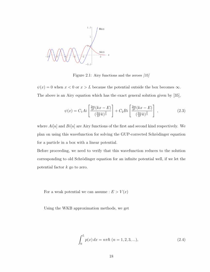
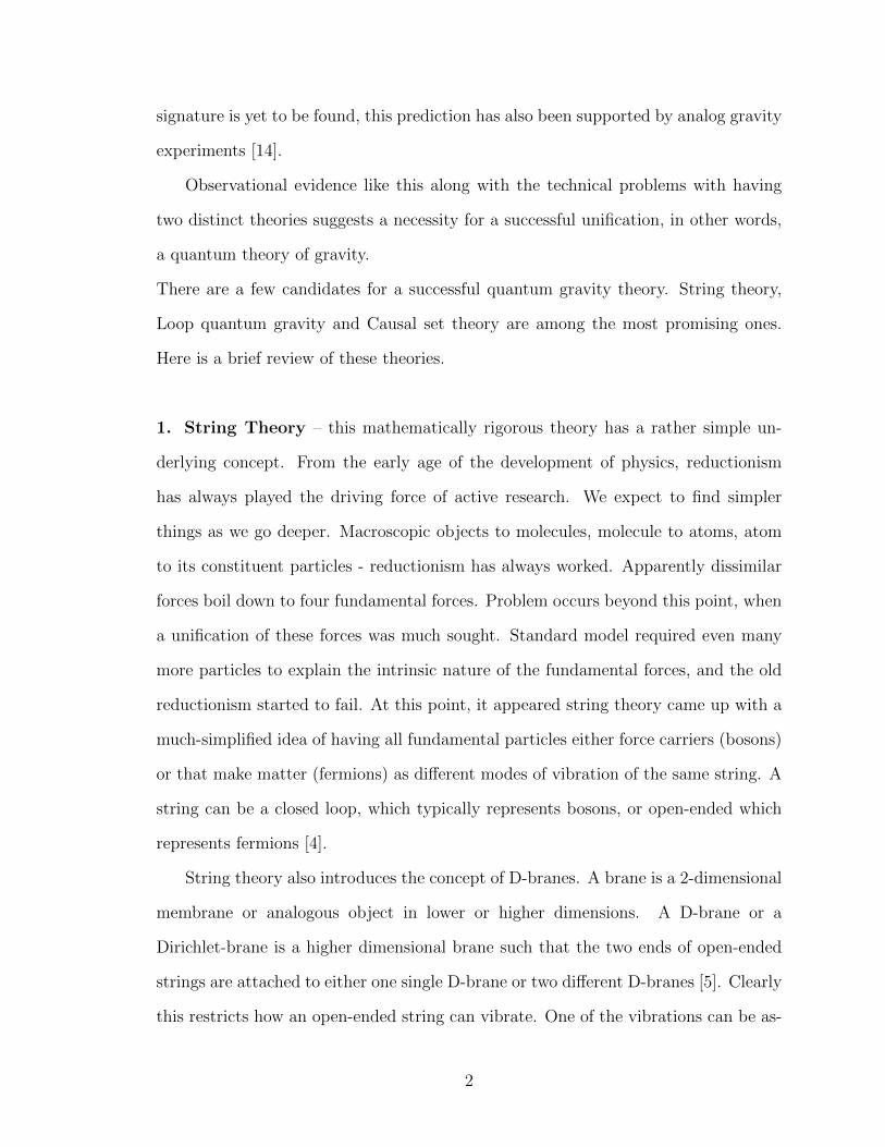
Figure 2.1: Airy functions and the zeroes [35]
ψ(x) = 0 when x < 0 or x > L because the potential outside the box becomes ∞.
The above is an Airy equation which has the exact general solution given by [35],
ψ(x) = C1Ai
[2m~2 (kx− E)
(2m~2 k)
23
]+ C2Bi
[2m~2 (kx− E)
(2m~2 k)
23
], (2.3)
where Ai[u] and Bi[u] are Airy functions of the first and second kind respectively. We
plan on using this wavefunction for solving the GUP-corrected Schrodinger equation
for a particle in a box with a linear potential.
Before proceeding, we need to verify that this wavefunction reduces to the solution
corresponding to old Schrodinger equation for an infinite potential well, if we let the
potential factor k go to zero.
For a weak potential we can assume : E > V (x)
Using the WKB approximation methods, we get
∫ L
0
p(x) dx = nπ~ (n = 1, 2, 3, ...), (2.4)
18

where p(x) ≡√
2m[E − V (x)].
This in turn gives the energy as,
E =1
4(√E0n ±
√E0n + ka)
⇒ En = E0n +
1
2ka+O
((1
E0n
)m), n = 1, 2, 3, .., (2.5)
where E0n = n2π2~2
2ma2.
In order to find the limiting forms of the energy and the wavefunction, we consider
the asymptotic form of the Airy functions.
Ai(−ξ) =1√πξ−14 sin(z +
π
4)
Bi(−ξ) =1√πξ−14 cos(z +
π
4), (2.6)
when ξ is very large.
Here z = 23ξ
32 and ξ ≡ ( 2m
~2 )13 (E−kx)
k23
.
The use of asymptotic forms is justified as ξ is very large in the limit k → 0.
z =2
3
((2m~2 )
13 (E − kx)
k23
) 32
≈ 2
3
(2m
~2
) 12
E32
(1
k− 3
2
x
E
)(for small k) ,
19
plugging this into Eq.(2.6) we get,
limk→0
Ai(−ξ) = limk→0
Ai
(−[(2m
~2)13E − kxk
23
])
=1√π
[(2m
~2
) 13 E − kx
k23
]−1/4
sin
{2
3
(2m
~2
) 12
E32
(1
k− 3
2
x
E
)+π
4
}
= H sin
{H1
(1
k− 3
2
x
E
)+π
4
}, (2.7)
where H = 1√π
[(2m~2 )
13E−kxk23
]− 14
and H1 = 23
(2m~2) 1
2 E32 .
Similarly,
limk→0
Bi(−ξ) = H cos
(H1
(1
k− 3
2
x
E
)+π
4
). (2.8)
Now, in this limit
Ai(−ξ) = H sin
([H1
k+π
4
]− 3
2H1
x
E
)= H sin
(H1
k+π
4
)cos
(3
2H1
x
E
)−H sin
(3
2H1
x
E
)cos
(H1
k+π
4
)
and
Bi(−ξ) = H cos
([H1
k+π
4
]− 3
2H1
x
E
)= H cos
(H1
k+π
4
)cos
(3
2H1
x
E
)+H sin
(H1
k+π
4
)sin
(3
2H1
x
E
)
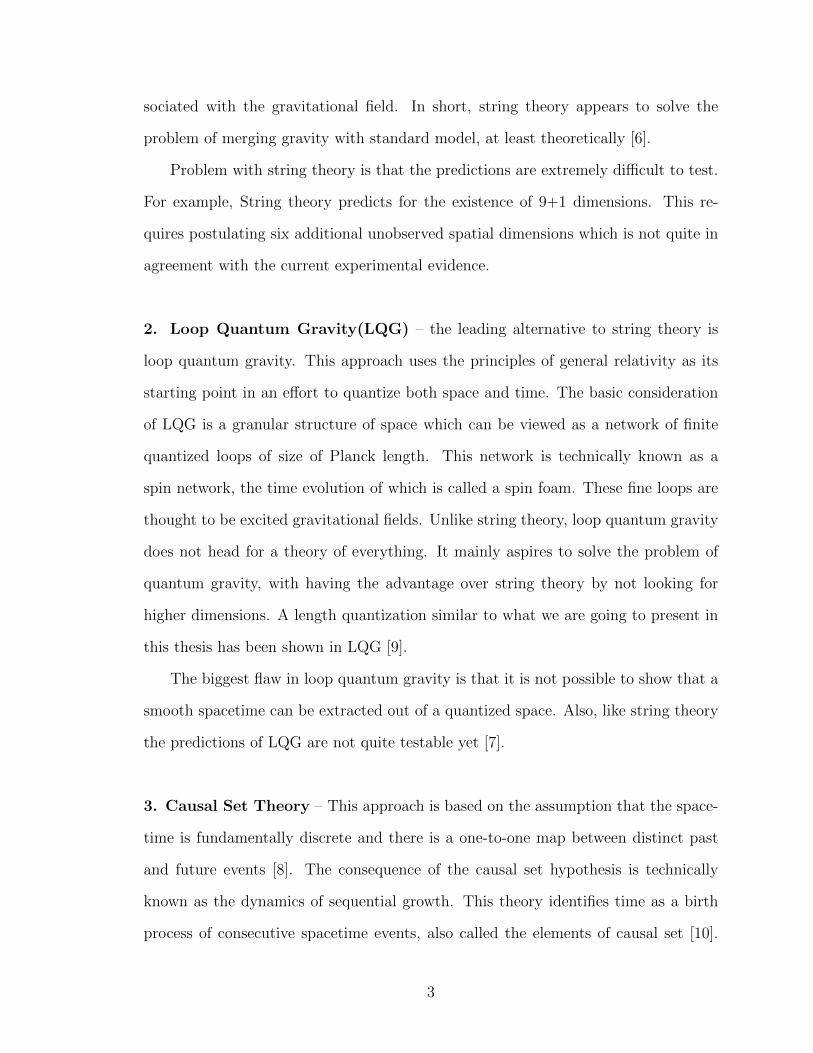
H ∼(E − kxk
23
)−1/4
= E−1/4k16
(1− kx
E
)−1/4
20
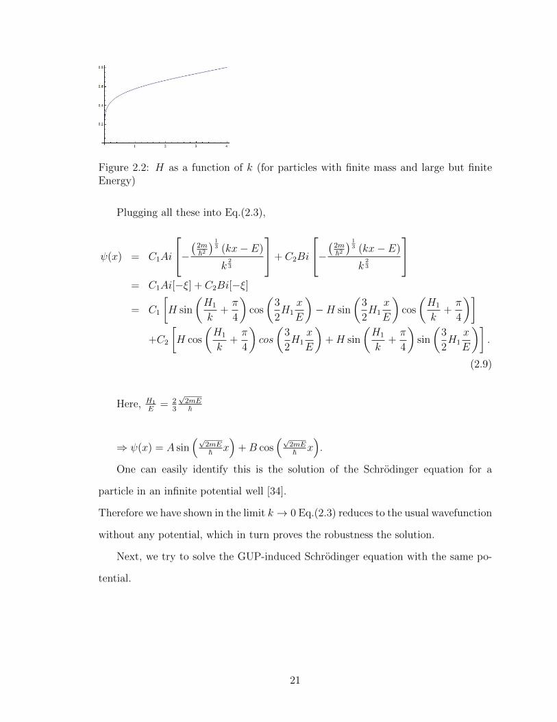
Figure 2.2: H as a function of k (for particles with finite mass and large but finiteEnergy)
Plugging all these into Eq.(2.3),
ψ(x) = C1Ai
−(2m~2) 1
3 (kx− E)
k23
+ C2Bi
−(2m~2) 1
3 (kx− E)
k23
= C1Ai[−ξ] + C2Bi[−ξ]
= C1
[H sin
(H1
k+π
4
)cos
(3
2H1
x
E
)−H sin
(3
2H1
x
E
)cos
(H1
k+π
4
)]+C2
[H cos
(H1
k+π
4
)cos
(3
2H1
x
E
)+H sin
(H1
k+π
4
)sin
(3
2H1
x
E
)].
(2.9)
Here, H1
E= 2
3
√2mE~
⇒ ψ(x) = A sin(√
2mE~ x
)+B cos
(√2mE~ x
).
One can easily identify this is the solution of the Schrodinger equation for a
particle in an infinite potential well [34].
Therefore we have shown in the limit k → 0 Eq.(2.3) reduces to the usual wavefunction
without any potential, which in turn proves the robustness the solution.
Next, we try to solve the GUP-induced Schrodinger equation with the same po-
tential.
21
2.3 GUP-corrected Schrodinger Equation with a One-dimensional Linear
Potential
Now that we have worked our way through a simple model with a weakly varying
gravitational potential, we can use this to a similar situation where we incorporate
GUP effects. We use the Hamiltonian given by Eq.(1.5), but in this case V (x) = kx
inside the box and V (x) =∞ ouside.
2.4 Solution of the GUP-corrected Schrodinger Equation:
Here. we are going to use the Schrodinger equation given by Eq.(1.7) with the
changes caused by this potential V (~r) = kx inside the box and V (~r) = ∞ outside.
Writing the Schrodinger equation with the modified Hamiltonian,
2iα~d3
dx3ψ +
d2
dx2ψ +
2m
~2(E − kx)ψ = 0 (2.10)
2.4.1 Perturbative Solutions
This is a third order linear differential equation. We hope to have the third
solution lead to a similar criterion [32] that would allow us to show the length of the
box can only assume some specific values.
Now, the above equation can be thought of as consisting of two parts,
part I: d2
dx2ψ + 2m
~2 (E − kx)ψ
and part II: 2iα~ d3
dx3ψ.
We intend to use a trial solution ψ1 = ψ0(E + cα, k, x), where the form of ψ0 is given
by Eq.(2.3), and claim that this is the solution we are looking for. It is to be noted
that ψ0(E, k, x) is the solution to part I
22
ψ1 = ψ0(E + cα, k, x)
= ψ0(E, k, x) + cαd
dEψ0(E, k, x) (2.11)
Substituting ψ1 in place of ψ in part I gives 0 + cα [terms containing ddEψ0].
Since we are not interested in terms containing α2, we can just use ψ1 = ψ0(E, k, x)
for part II which in turn yields α[terms containing derivatives of ψ0(E, k, x)].
So, we get
α[terms containing derivatives of ψ0(E, k, x)]+0 + cα [terms containing ddEψ0].
In order to have this expression to be zero for a value of c the terms in brackets
would have to be either independent of x or of the same leading order terms. In the
second case, we would argue that for small values of x we could neglect them and be
able to solve for c.
Combining all these along with Eqs.(2.10) and (2.11) we get
2iα~d3
dx3ψ0(E, k, x) + 2iα~cα
d3
dx3
(d
dEψ0(E, k, x)
)+ cα
d2
dx2
(d
dEψ0(E, k, x)
)+
2m
~2(E − kx)cα
d
dEψ0(E, k, x)
= α
[2i~
d3
dx3ψ0(E, k, x)
]+ cα
[d2
dx2
(d
dEψ0(E, k, x)
)+
2m
~2(E − kx)
d
dEψ0(E, k, x)
],
(2.12)
where
ψ0(E, k, x) = AAi(−ξ) +BBi(−ξ)
=A√πξ−1/4 sin
(2
3ξ
32 +
π
4
)+
B√πξ−1/4 cos
(2
3ξ
32 +
π
4
)(2.13)
23
ξ =(
2m~2) 1
3 k−23 (E − kx).
Now, plugging the derivatives (refer to appendix C) into Eq.(2.12),
α
[2i~
d3
dx3ψ0(E, k, x)
]+ cα
[d2
dx2
(d
dEψ0(E, k, x)
)+
2m
~2(E − kx)
d
dEψ0(E, k, x)
]= α
[2i~(dξ
dx
)3d3ψ0
dξ3
]+ cα
[(dξ
dx
)2dξ
dE
d3ψ0
dξ3+
2m
~2(E − kx)
dξ
dE
ψ0
dξ
].
(2.14)
For simplicity, we are going to use one of the two independent solutions ψI0 and
ψII0 as ψ0 in Eq.(2.14). Our intention is to check if coefficients of α and cα in the
above expression have at least the same leading order terms.
Using ψ0 = ψI0 ,
α
[2i~(dξ
dx
)3d3ψ0
dξ3
]+ cα
[(dξ
dx
)2dξ
dE
d3ψ0
dξ3+
2m
~2(E − kx)
dξ
dE
ψ0
dξ
]
= α
[2i~(−2m
~2
)k
(− 1√
π
[3
4ξ−1/4 sin
(2
3ξ3/2 +
π
4
)+ ξ5/4 cos
(2
3ξ3/2 +
π
4
)])]+cα
[(2m
~2
)2/3
k2/3
(2m
~2
)1/3 −k−2/3
√π
(3
4ξ−1/4 sin
(2
3ξ3/2 +
π
4
)+ ξ5/4 cos
(2
3ξ3/2 +
π
4
))
+2m
~2(E − kx)
(2m
~2
)1/3
k−2/3 1√π
(−1
4ξ−5/4 sin
(2
3ξ3/2 +
π
4
)+ ξ1/4 cos
(2
3ξ3/2 +
π
4
))]
24
= α(2i~)
(2m
~2
)(k√π
)3
4
((2m
~2
)1/3
k−2/3
)−1/4
(E − kx)−1/4 sin
(2
3ξ3/2 +
π
4
)+α(2i~)
(2m
~2
)(k√π
)((2m
~2
)1/3
k−2/3
)5/4
(E − kx)5/4 cos
(2
3ξ3/2 +
π
4
)−cα
(2m
~2
)(1√π
)3
4
((2m
~2
)1/3
k−2/3
)−1/4
(E − kx)−1/4 sin
(2
3ξ3/2 +
π
4
)−cα
(2m
~2
)(1√π
)((2m
~2
)1/3
k−2/3
)5/4
(E − kx)5/4 cos
(2
3ξ3/2 +
π
4
)− cα√
π
[1
4
(2m
~2
)11/12
k1/6 (E − kx)−1/4 sin
(2
3ξ3/2 +
π
4
)
−(
2m
~2
)17/12
k−5/6 (E − kx)5/4 cos
(2
3ξ3/2 +
π
4
)]
(2.15)
Since we are interested in the terms containing powers of x, it is to be noted that
the above expression would give the same leading order term for both α and cα.
Expanding the above expression using Taylor series and collecting coefficients of
25
x0 (ignoring terms containing x and higher orders of x),
α(2i~)
(2m
~2
)(k√π
)3
4
((2m
~2
)1/3
k−2/3
)−1/4
E−1/4 sin(ξ0 +
π
4
)+
((2m
~2
)1/3
k−2/3
)5/4
E5/4 cos(ξ0 +
π
4
)=
cα√π
2m
~2
3
4
((2m
~2
)1/3
k−2/3
)−1/4
E−1/4 sin(ξ0 +
π
4
)+
((2m
~2
)1/3
k−2/3
)5/4
E5/4 cos(ξ0 +
π
4
)+cα√π
[1
4
(2m
~2
)11/12
k1/6E−1/4 sin(ξ0 +
π
4
)−(
2m
~2
)17/12
k−5/6E5/4 cos(ξ0 +
π
4
)](2.16)
⇒ 2i~
[3
4
(2m
~2
)11/12
k7/6E−1/4 sin(ξ0 +
π
4
)+
(2m
~2
)17/12
k1/6E5/4 cos(ξ0 +
π
4
)]
= c
(2m
~2
)11/12
k1/6E−1/4 sin(ξ0 +
π
4
)(2.17)
⇒ c = 2i~34
(2m~2)11/12
k7/6E−1/4 sin(ξ0 + π
4
)+(
2m~2)17/12
k1/6E5/4 cos(ξ0 + π
4
)(2m~2)11/12
k1/6E−1/4 sin(ξ0 + π
4
)= 2i~
(3
4k +
E3/2
tan(ξ0 + π4)
√2m
~2
)(2.18)
where,
ξ0 =2
3
((2m
~2
)1/3
k−2/3E
)3/2
26
Now we are going to use the actual wavefunction in expression (3.31).
ψ0 = C1ψI0 + C2ψ
II0
For C1ψI0 part, (3.31) yields,
α(2i~)C1√π
[3
4
(2m
~2
)11/12
k7/6(E − kx)−1/4 sin
(2
3ξ3/2 +
π
4
)+
(2m
~2
)17/12
k1/6(E − kx)5/4 cos
(2
3ξ3/2 +
π
4
)]
= (cα)C1√π
[(2m
~2
)11/12
k1/6(E − kx)−1/4 sin
(2
3ξ3/2 +
π
4
)],
(2.19)
and for C1ψII0 part, (3.31) gives,
α(2i~)C2√π
[(2m
~2
)17/12
k1/6(E − kx)5/4 sin
(2
3ξ3/2 +
π
4
)−
3
4
(2m
~2
)11/12
k7/6(E − kx)−1/4 cos
(2
3ξ3/2 +
π
4
)]
= cαC2√π
[−(
2m
~2
)11/12
k1/6(E − kx)−1/4 cos
(2
3ξ3/2 +
π
4
)].
Combining them we get,
α(2i~)3
4
(2m
~2
)11/12
k7/6(E − kx)−1/4
[C1 sin
(2
3ξ3/2 +
π
4
)− C2 cos
(2
3ξ3/2 +
π
4
)]+
α(2i~)3
4
(2m
~2
)17/12
k1/6(E − kx)5/4
[C2 sin
(2
3ξ3/2 +
π
4
)+ C1 cos
(2
3ξ3/2 +
π
4
)]= cα
(2m
~2
)11/12
k1/6(E − kx)−1/4
[C1 sin
(2
3ξ3/2 +
π
4
)− C2 cos
(2
3ξ3/2 +
π
4
)].
(2.20)
Expanding the above equation using Taylor series and collecting coefficients of x0
27
(ignoring terms containing x and higher orders of x),
α(2i~)3
4
(2m
~2
)11/12
k7/6E−1/4[C1 sin(ξ0 +
π
4)− C2 cos(ξ0 +
π
4)]
+α(2i~)
(2m
~2
)17/12
k1/6E5/4[C2 sin(ξ0 +
π
4)− C1 cos(ξ0 +
π
4)]
= cα
(2m
~2
)11/12
k1/6E−1/4[C1 sin(ξ0 +
π
4)− C2 cos(ξ0 +
π
4)]
(2.21)
So,
c =
[(2i~)
3
4
(2m
~2
)11/12
k7/6E−1/4(C1 sin(ξ0 +
π
4)− C2 cos(ξ0 +
π
4))
+
α(2i~)
(2m
~2
)17/12
k1/6E5/4(C2 sin(ξ0 +
π
4)− C1 cos(ξ0 +
π
4))]÷[(
2m
~2
)11/12
k1/6E−1/4(C1 sin(ξ0 +
π
4)− C2 cos(ξ0 +
π
4))]
. (2.22)
Hence, the wavefunction is given by,
ψ1 = ψ0(E + cα, k, x)
= ψ0(E, k, x) + cαd
dEψ0(E, k, x)
= ψ0(E, k, x) + cαd
dξψ0(E, k, x)
dξ
dE
(2.23)
where ψ0(E, k, x), ddξψ0(E, k, x) and dξ
dEare given by Eqs.(C.1), (C.8) and (C.3) in
order(see appendix C).
It is to be noted here, that the above general solution consists two independent
solutions instead of three. The reason is that they are basically coming from a second
28
order differential equation (Eq.(2.2)). We just used them to find a general solution
of the actual third order differential equation as each of them satisfies it separately.
This perturbative solution is mathematically rigorous and complex to deal with.
In the next few sections, we will find the non-perturbative third solution and
develop a method to impose the boundary conditions on the general solution.
2.4.2 Non-perturbative Solution
The solution given in Eq.(2.23) is perturbative and based on the solutions of a
second order differential equation.
We assume the form of the third non-perturbative solution of the Eq.(2.10) as ψIII0 =
eiµx/`Pl .
If we can find a valid µ that satisfies Eq.(2.10) then we can write the general
solution as ψ(x) = C1ψI0 + C2ψ
II0 + C3ψ
III0 .
d
dxψIII0 =
(iµ
`Pl
)eiµx/`Pl =
iµ
`PlψIII0
d2
dx2ψIII0 = −
(µ
`Pl
)2
ψIII0
d3
dx3ψIII0 = −i
(µ
`Pl
)3
ψIII0
(2.24)
Plugging the above into Eq.(2.10) we get
2iα~(−i)(µ3
`3Pl
)− µ2
`2Pl
+2m
~2(E − kx) = 0
⇒ 2α0µ3 − µ2 = 0 (in the limit `Pl → 0)
⇒ µ2(2α0µ− 1) = 0
⇒ µ =1
2α0
29
Therefore, ψIII0 = eix/2α0`Pl = eix/2~α
2.4.3 General Solution
The general solution of the GUP-corrected Schrodinger equation (one-dimension)
is given by,
ψ(x) =A√π
[ξ−1/4 sin
(2
3ξ
32 +
π
4
)+
(2m
~2
)1/3
k−2/3cα
(−1
4ξ−5/4 sin
(2
3ξ3/2 +
π
4
)+
ξ1/4 cos
(2
3ξ3/2 +
π
4
))]+
B√π
[ξ−1/4 cos
(2
3ξ
32 +
π
4
)+(
2m
~2
)1/3
k−2/3cα
(−ξ1/4 sin
(2
3ξ3/2 +
π
4
)− 1
4ξ−5/4 cos
(2
3ξ3/2 +
π
4
))]+
Ceix/2~α
(2.25)
The constant C is such that |C| becomes zero in the limit α → 0 as the last term
should drop out in this limit. Phase of A can be absorbed in ψ so A can be treated
as a real constant.
In the limit k → 0, the above equation should reduce to the general solution of
the free particle (no field inside the box) GUP-corrected Schrodinger equation. Using
the asymptotic forms of the Airy functions in the same limit and ignoring terms
containing higher orders of α we can show that the wavefunction given by Eq.(2.25)
becomes,
ψ(x) = H A1 sin(3
2H1
x
E) +H A2 sin(
3
2H1
x
E) + (iα~)
[(η1 A1 − η2 A2) sin(
3
2H1
x
E)+
(η1 A2 + η2 A1) cos(3
2H1
x
E)+
]+ Ceix/2~α,
(2.26)
30
where
η1 = − 3
8√π
(2m
~2
)−1/12
k7/6(E − kx)−5/4 ≈ − 3
8√π
(2m
~2
)−1/12
k7/6E−5/4
η2 = − 3
2√π
(2m
~2
)5/12
k−1/6(E − kx)1/4 ≈ − 3
8√π
(2m
~2
)5/12
k−1/6E1/4
A1 = −A cos(H1
k+π
4) +B sin(
H1
k+π
4)
A2 = A sin(H1
k+π
4) +B cos(
H1
k+π
4) (see section 2.2)
Also, in the limit α → 0 Eq.(2.10) becomes a second order inhomogeneous dif-
ferential equation and in that case the solution given by Eq.(2.25) must become
ψ(x) containing the Airy functions only, i.e., limα→0 ψ(x) = A√πξ−1/4 sin
(23ξ
32 + π
4
)+
B√πξ−1/4 cos
(23ξ
32 + π
4
). This implies limα→0 |C| = 0
31
2.5 Boundary Conditions and Length Quantization
Now that we have the wavefunction corresponding to the GUP-induced Schrodinger
equation, we can use the boundary conditions ψ(0) = 0 and ψ(L) = 0. Like the case
without a gravitational potential [32], here we hope to find a new condition that
would lead to a restriction on the length of the box.
Imposing the boundary condition ψ(0) = 0 on Eq.(2.25) we get,
A√π
[ξ−1/40 sin
(2
3ξ
320 +
π
4
)+
(2m
~2
)1/3
k−2/3cα
(−1
4ξ−5/40 sin
(2
3ξ
3/20 +
π
4
)+
ξ1/40 cos
(2
3ξ
3/20 +
π
4
))]+
B√π
[ξ−1/40 cos
(2
3ξ
320 +
π
4
)+(
2m
~2
)1/3
k−2/3cα
(−ξ1/4
0 sin
(2
3ξ
3/20 +
π
4
)− 1
4ξ−5/40 cos
(2
3ξ
3/20 +
π
4
))]+ C = 0
(2.27)
Substituting for C in Eq.(2.25),
ψ(x) =A√π
[ξ−1/4 sin
(2
3ξ
32 +
π
4
)+
(2m
~2
)1/3
k−2/3cα
(−1
4ξ−5/4 sin
(2
3ξ3/2 +
π
4
)+
ξ1/4 cos
(2
3ξ3/2 +
π
4
))]+
B√π
[ξ−1/4 cos
(2
3ξ
32 +
π
4
)+(
2m
~2
)1/3
k−2/3cα
(−ξ1/4 sin
(2
3ξ3/2 +
π
4
)− 1
4ξ−5/4 cos
(2
3ξ3/2 +
π
4
))]
−eix/2~α A√π
[ξ−1/40 sin
(2
3ξ
320 +
π
4
)+
(2m
~2
)1/3
k−2/3cα
(−1
4ξ−5/40 sin
(2
3ξ
3/20 +
π
4
)+ ξ
1/40 cos
(2
3ξ
3/20 +
π
4
))]− eix/2~α B√
π
[ξ−1/40 cos
(2
3ξ
320 +
π
4
)+(
2m
~2
)1/3
k−2/3cα
(−ξ1/4
0 sin
(2
3ξ
3/20 +
π
4
)− 1
4ξ−5/40 cos
(2
3ξ
3/20 +
π
4
))].
(2.28)
32
Now, the remaining boundary condition ψ(L) = 0 implies,
eiL/2~α =f(ξL)
f(ξ0), (2.29)
where
f(ξL) =A√π
[ξ−1/4L sin
(2
3ξ
32L +
π
4
)+
(2m
~2
)1/3
k−2/3cα
(−1
4ξ−5/4L sin
(2
3ξ
3/2L +
π
4
)+
ξ1/4L cos
(2
3ξ
3/2L +
π
4
))]+
B√π
[ξ−1/4 cos
(2
3ξ
32L +
π
4
)+(
2m
~2
)1/3
k−2/3cα
(−ξ1/4
L sin
(2
3ξ
3/2L +
π
4
)− 1
4ξ−5/4L cos
(2
3ξ
3/2L +
π
4
))],
f(ξ0) =A√π
[ξ−1/40 sin
(2
3ξ
320 +
π
4
)+
(2m
~2
)1/3
k−2/3cα
(−1
4ξ−5/40 sin
(2
3ξ
3/20 +
π
4
)+
ξ1/40 cos
(2
3ξ
3/20 +
π
4
))]+
B√π
[ξ−1/40 cos
(2
3ξ
320 +
π
4
)+(
2m
~2
)1/3
k−2/3cα
(−ξ1/4
0 sin
(2
3ξ
3/20 +
π
4
)− 1
4ξ−5/40 cos
(2
3ξ
3/20 +
π
4
))],
and
ξL =
(2m
~2
)1/3
k−2/3(E − kL),
ξ0 =
(2m
~2
)1/3
k−2/3E,
33
Expanding f(ξL) and f(ξ0) w.r.t. α we get,
f(ξL) ≈ (2m
~2)−1/12k1/6(E − kL)−1/4
[A sin
(2
3
√2m
~2
(E − kL)3/2
k+π
4
)+
B cos
(2
3
√2m
~2
(E − kL)3/2
k+π
4
)]+O(α)
and
f(ξ0) ≈ (2m
~2)−1/12k1/6E−1/4
[A sin
(2
3
√2m
~2
E3/2
k+π
4
)+
B cos
(2
3
√2m
~2
E3/2
k+π
4
)]+O(α).
Thus,
eiL/2~α =(E − kL)−1/4
[A sin
(23
√2m~2
(E−kL)3/2
k+ π
4
)+B cos
(23
√2m~2
(E−kL)3/2
k+ π
4
)]E−1/4
[A sin
(23
√2m~2
E3/2
k+ π
4
)+B cos
(23
√2m~2
E3/2
k+ π
4
)]+O(α)
=
(1− kL
E
)−1/4 A sin(
23
√2m~2
(E−kL)3/2
k+ π
4
)+B cos
(23
√2m~2
(E−kL)3/2
k+ π
4
)A sin
(23
√2m~2
E3/2
k+ π
4
)+B cos
(23
√2m~2
E3/2
k+ π
4
)+O(α)
(2.30)
Writing B = |B|eiθB we get from the RHS of the above equation,
A sin(
23
√2m~2
(E−kL)3/2
k+ π
4
)+ |B|eiθB cos
(23
√2m~2
(E−kL)3/2
k+ π
4
)A sin
(23
√2m~2
E3/2
k+ π
4
)+ |B|eiθB cos
(23
√2m~2
E3/2
k+ π
4
)
=A sin
(23
√2m~2
(E−kL)3/2
k+ π
4
)+ |B| cos(θB) cos
(23
√2m~2
(E−kL)3/2
k+ π
4
)+ i|B| sin(θB) cos
(23
√2m~2
(E−kL)3/2
k+ π
4
)A sin(
(23
√2m~2
E3/2
k+ π
4
)) + |B| cos(θB) cos
(23
√2m~2
E3/2
k+ π
4
)+ i|B| sin(θB) cos
(23
√2m~2
E3/2
k+ π
4
)
34
(2.31)
Thus the real part the RHS of Eq.(2.30) is given by,
A2 sin(
23
√2m~2
E3/2
k+ π
4
)+A|B| cos(θB) cos
(23
√2m~2
E3/2
k+ π
4
)(A sin
(23
√2m~2
E3/2
k+ π
4
)+ |B| cos(θB) cos
(23
√2m~2
E3/2
k+ π
4
))2+ |B|2 sin2(θB) cos2
(23
√2m~2
E3/2
k+ π
4
)
× sin
(2
3
√2m
~2(E − kL)3/2
k+π
4
)
+
A|B| cos(θB) sin(
23
√2m~2
E3/2
k+ π
4
)+ |B|2 cos2(θB) cos
(23
√2m~2
E3/2
k+ π
4
)+ |B|2 sin2(θB) cos2
(23
√2m~2
E3/2
k+ π
4
)(A sin
(23
√2m~2
E3/2
k+ π
4
)+ |B| cos(θB) cos
(23
√2m~2
E3/2
k+ π
4
))2+ |B|2 sin2(θB) cos2
(23
√2m~2
E3/2
k+ π
4
)
× cos
(2
3
√2m
~2(E − kL)3/2
k+π
4
)
= A∗ sin
(2
3
√2m
~2(E − kL)3/2
k+π
4
)+B∗ cos
(2
3
√2m
~2(E − kL)3/2
k+π
4
)
Collecting real terms form both sides of the Eq.(2.30),
cos(L/2~α) =
(1− kL
E
)−1/4(A∗ sin
(2
3
√2m
~2
(E − kL)3/2
k+π
4
)+
B∗ cos
(2
3
√2m
~2
(E − kL)3/2
k+π
4
))(2.32)
Following the same argument in sec 2.2, the limit k → 0 the RHS the above
equation becomes
B1 cos
(√2mE
~2L
)− A1 sin
(√2mE
~2L
),
35
where A1 = H(A∗ cos
(H1
k+ π
4
)−B∗ sin
(H1
k+ π
4
))and
B1 = H(A∗ sin
(H1
k+ π
4
)+B∗ cos
(H1
k+ π
4
))(see page 19 for H,H1).
Without loss of generality, letting A1 = sin−1 θ and B1 = cos−1 θ for an arbitrary θ
we can write
cos(L/2~α) = cos θ cos
(√2mE
~2L
)− sin θ sin
(√2mE
~2L
)= cos
(√2mE
~2L+ θ
)
Referring to [32], we know that this implies L0
2α~ = pπ, p ∈ N, L0 being the length
of the box in flat space-time [32].
Since, L is a perturbation over L0 we can write,
L
2~α= P0(kL0) + pπ. (2.33)
It is to be noted that P0 is a small perturbative term and that L0
2α~ = p1π itself for
p1 ∈ N. P0 is a polynomial in kL derived from the RHS of Eq.(2.33).
We can write Eq.(2.35) as ,
L
2~α= f(k)p1π + pπ. (2.34)
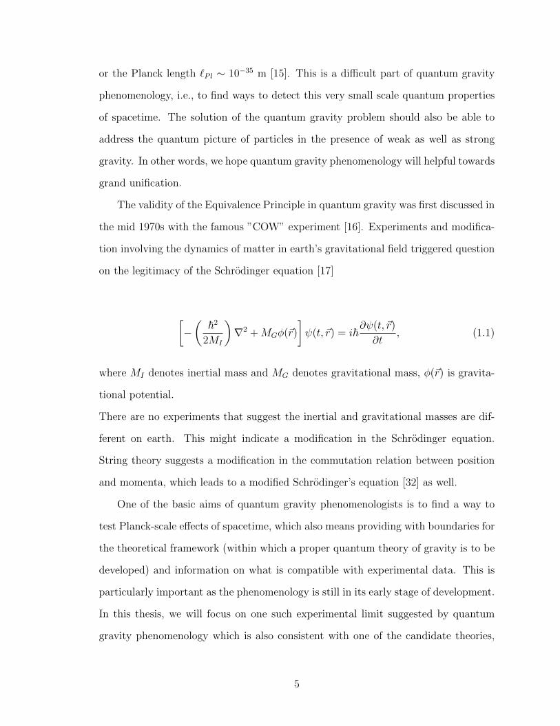
For each p we have a finite set of p1 values. As the perturbative term has to be
small, the number of p1 values, for each p, depends on the smallness of f(k). Fig.(3.3)
is included to provide a qualitative comparison. We can see we have a fine structure
(splitting) of the length quantization when gravity is involved compared to the much
simpler shell structure when gravity is not involved. This might remind one of the
similarities with the energy quantization of the hydrogen atom.
One might be interested to delve into the possible connection between the two.
Consideration of the significance of this apparent coincidence may further suggest
investigation of discreteness of space(time). Although the original Heisenberg Un-
36
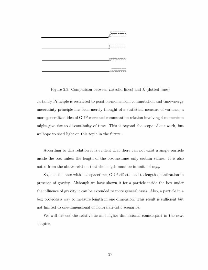
Figure 2.3: Comparison between L0(solid lines) and L (dotted lines)
certainty Principle is restricted to position-momentum commutation and time-energy
uncertainty principle has been merely thought of a statistical measure of variance, a
more generalized idea of GUP corrected commutation relation involving 4-momentum
might give rise to discontinuity of time. This is beyond the scope of our work, but
we hope to shed light on this topic in the future.
According to this relation it is evident that there can not exist a single particle
inside the box unless the length of the box assumes only certain values. It is also
noted from the above relation that the length must be in units of α0l0.
So, like the case with flat spacetime, GUP effects lead to length quantization in
presence of gravity. Although we have shown it for a particle inside the box under
the influence of gravity it can be extended to more general cases. Also, a particle in a
box provides a way to measure length in one dimension. This result is sufficient but
not limited to one-dimensional or non-relativistic scenarios.
We will discuss the relativistic and higher dimensional counterpart in the next
chapter.
37
Chapter 3
Discreteness of Space from GUP : Relativistic Case
As explained in section 1.4.2, we need a formalism to investigate the modification
of discreteness of space in a relativistic situation. The structure of spacetime does
not necessarily change depending on relativistic or non-relativistic test particles used
to probe it with, but it is quite fair that particles with speeds compared to the
speed of light can potentially reveal the structure better compared to less energetic
particles. In this chapter, we will have a closer look at the relativistic equivalent of the
Schrodinger equation and in particular the modification induced by GUP. Now, the
relativistic version of Schrodinger equation is Klein-Gordon equation. First we will
derive the GUP-version of the Klein-Gordon equation with a linear potential and then
try to solve it to obtain possible length quantization. Notwithstanding it’s relative
simplicity, Klein-Gordon equation has mathematical difficulties, especially when it
comes to dimensions higher than one, it’s much easier to resort to a more versatile
Dirac equation. In the consecutive sections we will try to solve the Dirac equation in
3-spatial dimensions and hope for getting a similar length quantization as in [33].
3.1 Klein-Gordon Equation in One dimension
The Klein-Gordon (sometimes known as Klein-Gordon-Fock) equation with no
38
field is given by [36],
(~2� +m2c2)ψ = 0, (3.1)
where � = 1c2
∂2
∂t2− ∇2, ~∇ = ∂
∂xi + ∂
∂yj + ∂
∂zk. It is basically same as Eq.(1.16). In
order to find the GUP-corrected Klein-Gordon equation we start from the Lorentz
invariant energy momentum equation,
pµpµ = m2c2
⇒ E2 = p2c2 +m2c4 (3.2)
Einstein summation notation is followed here. Now we replace the momentum with
the GUP-corrected momentum p = p0(1−αp0) and calculate the following quantities,
p2 = p20 − 2αp3
0
p0 ≡ −i~∂
∂;E ≡ i~
∂
∂t
⇒ p20 = −~2 ∂
2
∂x2; p3
0 = i~3 ∂3
∂x3.
Plugging these into Eq.(3.2) we get,
− c2~2∂2Ψ(x, t)
∂x2− c22αi~3∂
3Ψ(x, t)
∂x3+m2c4Ψ = −~2∂
2Ψ(x, t)
∂t2
Considering the stationary solutions only,
−c2~2∂2Ψ(x)
∂x2− 2c2α~3d
3Ψ(x)
dx3+m2c4Ψ = E2Ψ(x)
⇒ 2iα~d3ψ
dx3+d2ψ
dx2+
((E/m2c2)2 − 1)
~2m2c2ψ = 0 (3.3)
This is the GUP-corrected one-dimensional Klein-Gordon equation in flat space-time.
39
If we are to consider a relativistic particle in a one-dimensional box with a linearized
potential V (x) = kx, we can write the above equation in an equivalent form E ∼√−2iα~d3ψ
dx3− d2ψ
dx2+m2c4 + V (x) and then rewrite this as,
−2iα~d3ψ
dx3− d2ψ
dx2+m2c4ψ = (E − V (x))2 ψ
⇒ 2iα~d3ψ
dx3+d2ψ
dx2+
1
~2c2
(E2 −m2c4 − 2Ekx
)ψ = 0 (3.4)
If we can make the following connections between the variables in the above equation
and those in equation (2.10): 2iα~d3ψdx3
+ d2ψdx2
+ 2m~2 (E − kx)ψ = 0
2m
~2E → 1
~2c2(E2 −m2c4),
2Ek
~2c2→ 2mk
~2,
we get similar length quantization result as in section 2.5.
3.2 Dirac Equation
The three-dimensional version of Klein-Gordon equation suffers from non-locality
of differential operators. The term p2, when GUP is considered, becomes p2 =
p20 − 2αp3
0 = −~2∇2 + 2iα~3∇3. Now the second term is 2iα~3(∂2
∂x2+ ∂2
∂y2+ ∂2
∂z2
)3/2
.
Without going into the mathematical details of fractional calculus [37], we can simply
use the Dirac equation in order to avoid this problem.
The free particle Dirac equation is given by [39],
i∂Ψ
∂t=(βmc2 + c~α. ~P
)Ψ, (3.5)
40
where
β ≡ γ0 =
I2 0
0 −I2
(3.6)
and
αi ≡ γ0γi =
I2 0
0 −I2
0 σi
−σi 0
=
0 σi
σi 0
. (3.7)
σi, i=1(1)3 for the 3 spatial dimensions, are the Pauli spin matrices and they are
given by [38],
σx =
0 1
1 0
, σy =
0 −i
i 0
, σz =
1 0
0 −1
(3.8)
Here βmc2 + c~α. ~P is the Dirac Hamiltonian with no field. It is to noted that ~α is
distinct from the parameter α present in the GUP-corrected quantum mechanical
equations.
For an addition of a potential term in the form V (x) = kx we can write the Dirac
equation as,
i∂Ψ
∂t=(βmc2 + c~α. ~P + kxI4
)Ψ. (3.9)
Particularly, for one spatial dimension, say z, the GUP-corrected Dirac equation
becomes,
(−ic~αz
d
dz+ cα~2 d
2
dz2+ βmc2 + kzI4
)ψ(z) = Eψ(z). (3.10)
Unlike Eq(3.6), the above is an eigenvalue equation.
41
3.3 Solution of Dirac Equation
Rewriting Eq.(3.11) we get,
(−ic~αz
d
dz+ cα~2 d
2
dz2+ βmc2 − E + kz
)ψ(Z) = 0. (3.11)
3.3.1 Perturbative solution
In order to solve the above equation we develop the following formalism.
The differential operator in Eq.(3.12) can be thought of composed of two components
−ic~αz ddz + cα~2 d2
dz2+ βmc2 − E and kz. This second component can be considered
as a perturbative term as both k and z are small. The solution to the first being
already known [33], we can add a small perturbative term to that solution in order
to get the complete solution of Eq.(3.12).
Let us use a trial solution of the form ψ = ψ(κ + C1k) which can also be written as
ψ = ψ1(k = 0) + C1kddκψ1(k = 0) to the first order of approximation since a small k
perturbative term seems logical to use.
Here, ψ1(k = 0) = N1eiκz
χ
rσzχ
.
κ = κ0 + α~κ20, κ0 being the wave number that satisfies E2 = (~κ0)2 + (mc2)2, r =
~κ0cE+mc2
and χ†χ = I. Now, we re-write Eq.(3.12)using the above.
(−ic~αz
d
dz+ cα~2 d
2
dz2+ βmc2 − E + kz
)N1eiκz
χ
rσzχ
+ C1kizN1eiκz
χ
rσzχ
= 0
(3.12)
42
As we have discussed above,
(−ic~αz
d
dz+ cα~2 d
2
dz2+ βmc2 − E
)N1e
iκz
χ
rσzχ
= 0.
Also, since k is very small, (kz)
kizN1eiκz
χ
rσzχ
= 0
In that case, Eq.(3.13) reduces to,
(−ic~αz
d
dz+ cα~2 d
2
dz2+ βmc2 − E
)C1kizN1e
iκz
χ
rσzχ
+ kzN1eiκz
χ
rσzχ
= 0
⇒ C1
(−ic~αz
d
dz+ cα~2 d
2
dz2+ βmc2 − E
)izψ1 = −zψ1
(3.13)
If we can find a valid C1 for the above, we can claim ψ1 is a solution of Eq.(3.13)
which in turn means ψ is a solution of Eq. (3.12).
C1
(c~αz
d
dz(zψ1) + icα~2
d2
dz2(zψ1) +mc2β(izψ1)− iE(zψ1)
)= −zψ1
(3.14)
⇒ C1
(c~+ ic~κz)
0 σz
σz 0
+ imc2z
I2 0
0 −I2
− (2cακ~2 + izE + icα~2z) I2 0
0 I2
ψ =
−zψ
43
⇒
(imc2z − 2cακ~2 − izE − icακ~2z
)I2 c~(1 + κz)σz
c~(1 + κz)σz(−imc2z − 2cακ~2 − izE − icακ~2z
)I2
= − z
C1ψ1
(3.15)
This is clearly an eigenvalue equation the associated matrix of which must be
singular in order to have nontrivial solutions. In other words,
∣∣∣∣∣∣∣∣∣(zC1
+ imc2z − 2cακ~2 − izE − icακ~2z)I2 c~(1 + iκz)σz
c~(1 + iκz)σz(zC1− imc2z − 2cακ~2 − izE − icακ~2z
)I2
∣∣∣∣∣∣∣∣∣ = 0
(3.16)
Clearly, this is a characteristic equation in z/C1, which by expanding the determinant,
can be written as,
(z
C1
− 2icακ~2 − iz(E + cακ~2)
)2
− (imc2z)2 − c2~2(1 + iκz)2 = 0.
For small z (which is quite reasonable considering the fact that the dimension we are
dealing with is close to the Planck length), the above equation gives,
(z
C1
− 2cακ~)2 − 2z(z
C1
− 2cακ~)(E + cακ~2)− ~2c2 − 2ic2~2κz = 0
⇒ 4cακ~2z
C1
= 4icακ~2z(E + cακ~2)− ~2c2(1 + 2iκz)
⇒ 1
C1
=4iακz(E + cακ~2)− (c+ 2icκz)
4ακz
⇒ 1
C1
= −c+ 2iακz (c(1− 2ακ~2)− 2E)
4ακz
⇒ C1 = − 4ακ
c/z + 2iακ (c(1− 2ακ~2)− 2E)(3.17)
44
So, the solution of Eq.(3.12) is given by,
ψ = N1eiκz
χ
rσzχ
− 4ακ
c/z + 2iακ (c(1− 2ακ~2)− 2E)kizN1e
iκz
χ
rσzχ
=
(1− 4ikακz
c/z + 2iακ (c(1− 2ακ~2)− 2E)
)N1e
iκz
χ
rσzχ
(3.18)
The above is the perturbative wavefunction corresponding to the GUP-corrected
Dirac equation.
3.3.2 Non-perturbative solution
Let us suppose the non-perturbative solution has the form
ψNP = eiµz/`Pl
χ
σzχ
(3.19)
Now, plugging this solution into Eq.(3.12),
(−ic~αz
d
dz+ cα~2 d
2
dz2+mc2β − E + kz
)eiµz/`Pl
χ
σzχ
= 0
⇒ µ(1− α0µ) = 0
⇒ µ
`Pl=
1
α~
3.4 Boundary Condition and Length Quantization
It is to be noted that GUP-induced Dirac equation with a linearized potential is a
second order inhomogeneous differential equation. Also because the matrix associated
is of order 4×4, one can expect eight linearly independent solutions. Here, we wish to
restrict ourselves to positive energy solutions only. In that case we have four linearly
45
independent solutions given by,
ψ1 = N1
(1− 4ikακz
c/z + 2iακ (c(1− 2ακ~2)− 2E)
)eiκz
χ
rσzχ
(3.20)
ψ2 = N2eiz/α~
χ
σzχ
(3.21)
where χ is a normalized spinor, meaning χ†χ = 1. χ could be chosen as
1
0
for
spin up state or
0
1
for spin down state or any linear combination of the two.
It is to be noted that similar to the case of GUP-induced Schrodinger equation this
non-perturbative solution here should disappear in the limit α → 0 as we should
get our old Dirac equation back in the same limit which is essentially a first order
differential equation.
Now, if we try to impose the boundary conditions on the wavefunction by letting
the gravitational potential go to infinity just outside the box, like we did in the non-
relativistic case, the so-called Klein paradox occurs. In other words, the flux of the
reflected plane wave on the infinite walls (boundaries) of the box appears higher than
that of the incident wave [40].
In order to avoid this situation, we resort to the famous MIT bag model of confined
quarks once again [41].
As discussed in [33], the mass of the relativistic particle of interest is considered as a
function of z,
m(z) =
M if z ≤ 0
m 0 ≤ z ≤ L
M z ≥ L,
(3.22)
46
where m is the rest mass of the particle and M is a constant. In order to have an
equivalent picture as infinite potential walls we will let M eventually grow infinitely
large causing the particle trapped inside the box. The advantage of this method
is that now we have the opportunity to consider the solution of the GUP-induced
Dirac equation separately in three regions, region I associated with z ≤ 0, II with
0 ≤ z ≤ L and III with z ≥ L. Now, in all of these three regions the wavefunction
should assume the same form of a linear combination of the perturbative and non-
perturbative solutions. Although, inside the box, i.e., in region II one might consider
an incident and a reflected wave whereas outside the box, it would suffice to consider
only one wave travelling outward from the walls. It should be a plane wave travelling
left in region I and travelling right in region III.
So, with reference to [33], the wavefunctions in the three regions are given by,
ψI = A
(1 +
4ikακ′z
c/z − 2iακ′ (c(1 + 2ακ′~2)− 2E)
)e−iκ
′z
χ
−Rσzχ
+Geizα~
χ
σzχ
(3.23)
ψII = B
(1− 4ikακz
c/z + 2iακ (c(1− 2ακ~2)− 2E)
)eiκz
χ
rσzχ
+C
(1 +
4ikακz
c/z − 2iακ (c(1 + 2ακ~2)− 2E)
)e−iκz
χ
−rσzχ
+Fe
izα~
χ
σzχ
47
(3.24)
ψIII = D
(1− 4ikακ
′z
c/z + 2iακ′ (c(1− 2ακ′~2)− 2E)
)eiκ′z
χ
Rσzχ
+Heizα~
χ
σzχ
,
(3.25)
where κ′
= κ′0 + α~κ′0
2, E =
√(~κ′0c)2 + (Mc2)2 and R =
~κ′0cE+Mc2
. To give the above
wavefunctions a little simpler form, let us have
ρ1 =
(1− 4ikακz
c/z + 2iακ (c(1− 2ακ~2)− 2E)
)ρ2 =
(1 +
4ikακz
c/z − 2iακ (c(1 + 2ακ~2)− 2E)
)ρ′
1 =
(1− 4ikακ
′z
c/z + 2iακ′ (c(1− 2ακ′~2)− 2E)
)ρ′
2 =
(1 +
4ikακ′z
c/z − 2iακ′ (c(1 + 2ακ′~2)− 2E)
),
and re-write the wavefunctions as,
ψI = Aρ2′e−iκ
′z
χ
−Rσzχ
+Geizα~
χ
σzχ
(3.26)
ψII = Bρ1eiκz
χ
rσzχ
+ Cρ2e−iκz
χ
−rσzχ
+ Feizα~
χ
σzχ
(3.27)
ψIII = Dρ′
1eiκ′z
χ
Rσzχ
+Heizα~
χ
σzχ
. (3.28)
Following the same line of argument as in [33], we can say that when M is very large,
48
E2 − M2c4 < 0 which means κ′0 =
√E2
c2−M2c2/~ is imaginary. So, in the limit
M → ∞, κ′0 → i∞ and κ
′= i
~
√Mc2 − E2
c2− α
~ (M2c2 − E2
c2) is a very large com-
plex number. It follows that e−iκ′z =
(e−|z|~
√Mc2−E2
c2
)(e−
iα|z|~ (M2c2−E
2
c2)
)→ 0 and
eiκ′z =
(e−
z~
√Mc2−E2
c2
)(e−
iαz~ (M2c2−E
2
c2)
)→ 0 in the limit M → ∞. This is simply
because the modulus of each of these complex numbers becomes zero in this limit.
Moreover, both ρ′1 and ρ2
′ ∼ 1−O(i/κ′0) so they become unity in the limit M →∞.
So, in the limit M →∞ the terms containing A and D becomes zero. As for the the
terms associated with G and H, the fluxes are nonzero [33] which means we have to
set G = 0 and H = 0. Now, in the limit α→ 0 and k → 0 Eq.(3.12) becomes the old
Dirac equation without any effects of GUP. As we can see from Eq.(3.27), this means
ρ1 and ρ2 must become unity which is evident. Moreover, this means the term with
F must vanish in the limit α → 0, which compels us to choose F ∼ αs, s > 0. This
will also take care of the possible blowup of the exponential term, especially if we let
s ≥ 10 F will decrease reasonably faster than e1α increases. This lower bound of s is
based on a numerical comparison between α and s calculated in MapleTM16 .
Finally, without loss of generality we can choose B = 1 like in [33] but the selec-
tion of C is to be determined from its relationship with B, which we are about to
figure out.
The usual boundary conditions that one would expect for the Schrodinger equation,
viz., ψII(z = 0) = 0ψII(z = L) do not quite work in this case as they would make the
wavefunction inside the box vanish. Alternatively, we use the MIT bag model which
is having the outward flux of the Dirac current at the boundaries z = 0 and z = L
49
zero [40]. Equivalently one can write [41],
iγ3ψ = ψ, at z = 0 (3.29)
iγ3ψ = −ψ, at z = L. (3.30)
Using ψ = ψII in Eq.(3.29) we get,
iγ3ψII(0) = ψII(0)
⇒ iBρ1
0 σz
−σz 0
χ
rσzχ
+ iCρ2
0 σz
−σz 0
χ
−rσzχ
+iF
0 σz
−σz 0
χ
σzχ
= Bρ1
χ
rσzχ
+ Cρ2
χ
−rσzχ
+ F
χ
σzχ
Collecting terms,
irBρ1 − irCρ2 + iF = Bρ1 + Cρ2 + F
⇒ ir(ρ1B − ρ2C) = ρ1B + ρ2C + F (1− i)
⇒ ir(ρ1B − ρ2C) = ρ1B + ρ2C + F√
2e−iπ/4
⇒ ρ1B + ρ2C + F′e−iπ/4
ρ1B − ρ2C= ir, (3.31)
where F′=√
2F .
50

From the other boundary condition (Eq. (3.30)),
iBρ1eiκL
0 σz
−σz 0
χ
rσzχ
+ iCρ2e−iκL
0 σz
−σz 0
χ
−rσzχ
+iFeiL/α~
0 σz
−σz 0
χ
σzχ
= −Bρ1e
iκL
χ
rσzχ
− Ce−iκLρ2
χ
−rσzχ
− FeiL/α~ χ
σzχ
Collecting terms,
irBρ1eiκL − irCρ2e
−iκL + iFeiL/α~ = −Bρ1eiκL − Cρ2e
−iκL − FeiL/α~
⇒ ρ1BeiκL + ρ2Ce
−iκL + F′ei(L/α~+π/4)
ρ1BeiκL − ρ2Ce−iκL= −ir, (3.32)
In order to establish a relationship between B and C let us start with Eq.(3.31),
ρ1B + ρ2C + F′e−iπ/4
ρ1B − ρ2C= ir
⇒ C =ρ1
ρ2
ir − 1
ir + 1B − F ′ e−iπ/4
ρ2(ir + 1). (3.33)
It is to be noted that ir−1ir+1
is unimodular as it can be expressed as
ir−1ir+1
= −r2+1−2ir−r2−1
= r2−1r2+1
+ i 2rr2+1
= eδ where
δ = tan−1(2r
r2 − 1). (3.34)
ρ2 increases with k, the linear potential term, and ρ2 → 1 as k → 0. So, Eq.(3.33)
can be re-written as,
C =|ρ1||ρ2|
ei(θρ1−θρ2 )eiδB +O(α), (3.35)
51
and
|C| = |B| |ρ1||ρ2|
+O(α). (3.36)
Clearly, in the limit k → 0, ρ1 → 1 = ρ2 = 1 and θρ1 = θρ2 = 0.
To find a condition on the length of the box, we will consider the other boundary
condition. We get from Eq. (3.32),
ρ1BeiκL + ρ2Ce
−iκL + F′ei(L/α~+π/4) = −irρ1Be
iκL + irρ2Ce−iκL
⇒ ρ1(ir + 1)BeiκL + F′ei(L/α~+π/4) = ρ2(ir − 1)Ce−iκL (3.37)
Now, if we substitute C = |ρ1||ρ2|e
i(θρ1−θρ2 )eiδB in Eq.(3.37) we get,
ρ1(ir + 1)BeiκL + F′ei(L/α~+π/4) = ρ2(ir − 1)
|ρ1||ρ2|
ei(θρ1−θρ2 )e−iκLeiδB
⇒ Be2iκL + F′ ei(L/α~+π/4)
ρ1(ir + 1)=ir − 1
ir + 1eiδB
(3.38)
Choosing B = 1 and substituting eiδ = ir−1ir+1
in Eq.(3.38),
e2iκL =
(ir − 1
ir + 1
)2
− F ′ ei(L/α~+π/4)
ρ1(ir + 1)(3.39)
⇒ e2ikL = e2i tan−1
(2r
r2−1
)− F ′ e
i(L/α~+π/4)
ρ1(ir + 1)(3.40)
⇒ κL = tan−1
(2r
r2 − 1
)+O(ln(α)) (3.41)
52
Now, from Eq.(3.37)
ρ1(ir + 1)BeiκL + F′ei(L/α~+π/4) = ρ2(ir − 1)Ce−iκL
⇒ ei(L/α~+π/4) =
ρ1(ir − 1)
(ei(δ−κL)−e
i
(κL−tan−1
(2r
r2−1
)))F ′
(3.42)
It follows from Eq.(3.42),
L
α~= −π
4+ arg
ρ1(ir − 1)
(ei(δ−κL)−e
i
(κL−tan−1
(2r
r2−1
)))F ′
+ 2nπ, n ∈ N
(3.43)
It is to be noted unlike the case without the presence of gravity [33] δ and κL here
are not the same as given by Eq.(3.34) and (3.41). They become the same in the
limit k → 0.
Thus, a relativistic particle can be trapped in a one-dimensional box, with a linearized
gravitational potential inside, only if the length of the box is quantized and the nature
of quantization is given by the above equation.
One would expect in the limit k → 0 Eq.(3.39) to reduce to the old quantization rule
given by Eq. (27) in [33]. To verify this we begin with Eq. (22) in [33] which on
slight algebraic rearrangement gives,
e−iπ/4 =(ir − 1)− (ir + 1)eiδ
F ′(3.44)
53
Now, if we let k go to zero, ρ→ 1, κL→ δ. So the RHS of Eq.(3.42) becomes,
ρ1(ir − 1)
(ei(δ−κL)−e
i
(κL−tan−1
(2r
r2−1
)))F ′
=(ir − 1)− (ir + 1)eiδ
F ′(3.45)
So, comparing Eqs.(3.42),(3.44) and (3.45) we can write (in the limit k → 0),
ei(L/α~+π/4) = e−iπ/4
⇒ L
α~= −π
2+ 2nπ, n ∈ N, (3.46)
which is nothing but the length quatization rule for a relativistic particle in a box
without the influence of gravity (see Eq.(1.22)).
3.5 Dirac Equation in Three Dimensions
As discussed in section 1.4.3, discreteness of space for two and three dimensions
has been shown without gravity. In this section we consider the generalized Dirac
equation for three dimensions and extend the result for a box with a slowly varying
gravitational potential inside, which can be linearized as before.
Let us consider a box defined by 0 ≤ xi ≤ Li, i = 1(1)d, d being the dimension of the
box, i.e., d = 1, 2 or 3. This box can be one two or three-dimensional. Now, we have
a linear potential inside as before. Without loss of generality, we can consider the
direction in which the potential changes as our x-direction. The Dirac Hamiltonian
54
with a potential term can be written as
H = ~cα.~p+ βmc2 + V (~r)I
= c (αxpx + αypy + αzpz) + βmc2 + kxI
= c(αxp0x + αyp0y + αzp0z − αp2
0x − αp20y − αp2
0z
)+ βmc2 + kxI
(3.47)
It is to be noted that we used the GUP-corrected momenta, pi = p0−αp0, i = 1, .., 3,
where p0i = −i~ ddxi
and followed Dirac prescription, i.e., we replaced p0i by αip0i and
used α2i = I.
We are going to use the same ansatz here as in [33] (see section 1.4.3) . The Dirac
Hamiltonian here is same as that in [33] except for a potential along x-axis. We
already know the modified perturbative and non-perturbative wavefunctions under
the influence of a one-dimensional linear potential. So, combining Eqs.(3.20), (3.21)
in section 3.4 and Eq. (30) and (31) in [33] we can write the two independent wave-
functions corresponding to the above Hamiltonian,
ψ1 = N1ρjei~κ.~r
χ
rκ.~σχ
(3.48)
ψ2 = N2ei q.~rα~
χ
q.~σχ
, (3.49)
j = 1, 2 for wavefronts going rightward and leftward respectively.
ρ1 =
(1− 4ikακ1x
c/x+ 2iακ1 (c(1− 2ακ~2)− 2E)
)ρ2 =
(1 +
4ikακ1x
c/x− 2iακ1 (c(1 + 2ακ1~2)− 2E)
).
Now, just like we did in section 3.4, here also we distinguish between regions in-
55
side and outside the box, but unlike the one-dimensional case, here we consider the
wavefunction inside the box only. We impose the boundary conditions on this wave-
function by resorting to the MIT bag model again.
Let us consider the following general form of a wavefunction inside the box going in
a particular direction,
Ψ = ρε1+
1−ε12
1 ρ1−ε1
22 e
i
(d∑i=1
εiκixi+1−εi
2δi
) χ
rd∑i=1
εiκiσiχ
, (3.50)
where δi (i = 1(1)d) and d = 1, 2, 3. The highest value of d clearly depends on how
many spatial dimensions the box has. There are 2d possible individual wavefunctions,
for all possible combinations with εi(i = 1, .., d) = ±1. The wavefunction inside the
box would be a superposition of those 2d kets and Fψ2,
ψ =
[d∏i=1
(ρδi11 eiκixi + ρδi12 e−i(κixi−δi)
)+ Fei
q.~rα~
]χ
d∑j=1
[d∏i=1
(ρδi11 eiκixi + (−1)δijρδi12 e−i(κixi−δi)
)rκj + Fei
q.~rα~ qj
]σjχ
,
(3.51)
where δij is the usual Kronecker delta. The number of terms in row I is 2d + 1 and
that in row II is (2d + 1)× d.
3.6 Boundary Conditions
The MIT bag model boundary conditions are,
iγlψ = ψ, at xl = 0 (3.52)
iγlψ = −ψ, at xl = L, (3.53)
56
for l = 1, .., d. Like the one-dimensional case, these conditions make sure the flux of
the Dirac probability current through any of the six surfaces is zero. This way we
can also avoid writing six different wavefunctions for six different regions outside the
box.
Now, the above conditions imposed together on the wavefunction given by Eq.(3.51)
for any xl gives,
id∑j=1
[d∏i=1
(ρδi11 eiκixi + (−1)δijρδi12 e−i(κixi−δi)
)rκjσlσj + Fei
q.~rα~ qjσlσj
]χ
−i[d∏i=1
(ρδi11 eiκixi + ρδi12 e−i(κixi−δi)
)+ Fei
q.~rα~
]σlχ
= ±
[d∏i=1
(ρδi11 eiκixi + ρδi12 e−i(κixi−δi)
)+ Fei
q.~rα~
]χ
d∑j=1
[d∏i=1
(ρδi11 eiκixi + (−1)δijρδi12 e−i(κixi−δi)
)rκj + Fei
q.~rα~ qj
]σjχ
.
(3.54)
Equating row I we get,
id∑j=1
[d∏i=1
(ρδi11 eiκixi + (−1)δijρδi12 e−i(κixi−δi)
)rκjσlσj + Fei
q.~rα~ qjσlσj
]
= ±d∏i=1
(ρδi11 eiκixi + ρδi12 e−i(κixi−δi)
)+ Fei
q.~rα~
⇒ id∏i=1
(ρδi11 eiκixi + (−1)δilρδi12 e−i(κixi−δi)
)rκl + iFei
q.~rα~ qj
+id∑
j=16=l
[d∏i=1
(ρδi11 eiκixi + (−1)δijρδi12 e−i(κixi−δi)
)rκjσlσj + Fei
q.~rα~ qjσlσj
]
= ±d∏i=1
(ρδi11 eiκixi + ρδi12 e−i(κixi−δi)
)+ Fei
q.~rα~ .
57
A little rearrangement yields,
d∏i=1
(ρδi11 eiκixi + ρδi12 e−i(κixi−δi)
)+ Fei
q.~rα~
= ±
[i
d∏i=1
(ρδi11 eiκixi + (−1)δilρδi12 e−i(κixi−δi)
)rκl + iFei
q.~rα~ qj
+id∑
j=16=l
(d∏i=1
(ρδi11 eiκixi + (−1)δijρδi12 e−i(κixi−δi)
)rκj + Fei
q.~rα~ qj
)σlσj
],
(3.55)
and equating row II,
−i
[d∏i=1
(ρδi11 eiκixi + ρδi12 e−i(κixi−δi)
)+ Fei
q.~rα~
]σl
= ±d∑j=1
[d∏i=1
(ρδi11 eiκixi + (−1)δijρδi12 e−i(κixi−δi)
)rκj + Fei
q.~rα~ qj
]σj.
Post-multiplying by iσl,
d∏i=1
(ρδi11 eiκixi + ρδi12 e−i(κixi−δi)
)+ Fei
q.~rα~
= ±
[i
d∏i=1
(ρδi11 eiκixi + (−1)δilρδi12 e−i(κixi−δi)
)rκl + iFei
q.~rα~ ql
+id∑
j=16=l
(d∏i=1
(ρδi11 eiκixi + (−1)δijρδi12 e−i(κixi−δi)
)rκj + Fei
q.~rα~ qj
)σjσl
].
(3.56)
These two equations are almost the same except for the order of multiplication of σl
58
and σj in the RHS. Adding Eq. (3.55) and Eq. (3.56),
2d∏i=1
(ρδi11 eiκixi + ρδi12 e−i(κixi−δi)
)+ 2Fei
q.~rα~
= ±2id∏i=1
(ρδi11 eiκixi + (−1)δilρδi12 e−i(κixi−δi)
)rκl ± 2iFei
q.~rα~ ql
±id∑
j=16=l
[(d∏i=1
(ρδi11 eiκixi + (−1)δijρδi12 e−i(κixi−δi)
)rκj + Fei
q.~rα~ qj
)(σlσj + σjσl)
].
(3.57)
Finally, using the anti-commutator {σl, σj} = 0 we can write,
d∏i=1
(ρδi11 eiκixi + ρδi12 e−i(κixi−δi)
)+ Fei
q.~rα~
= ±id∏i=1
(ρδi11 eiκixi + (−1)δilρδi12 e−i(κixi−δi)
)rκl ± iFei
q.~rα~ ql
(3.58)
In order to substitute xl = 0 and xl = L in the above equation we need terms con-
taining (xl, κl, δl) and rest of the variables depending on a different i separately. The
easiest way to get such terms is to divide Eq.(3.58) by a product of terms that contain
all indices but i = l. Now the structure of this product depends on whether we want
to find a restriction on xl or on xi 6=l.
3.6.1 Case 1 : Length quantization along x axis
In this case, l = 1, i.e., xl = x. Dividing Eq.(3.58) by
59
fl(xi, κi, δi) =d∏
i=16=l
(eiκixi + e−i(κixi−δi)
)we get,
ρ1eiκ1x + ρ2e
−i(κ1x−δ1) + f−1lFei
q.~rα~
= ±i(ρ1e
iκ1x − ρ2e−i(κ1x−δ1)
)rκ1 ± if−1
lFei
q.~rα~ q1 (3.59)
Eq.(3.59), at x = 0, yields,
ρ1 + ρ2eiδ1 + f−1
lF = i(ρ1 − ρ2e
iδ1)rκ1 + if−1lF q1
⇒ eiδ1(irκ1 + 1)ρ2 = (irκ1 − 1)ρ1 + f−1lF′e−iθ1 , (3.60)
where F′
=√
1 + q12F and θ1 = tan−1(q1). Although we used the index l, f−1
lis
nothing but f−11
, i.e., evaluated at xl = x.
Eq.(3.59), at x = L1, yields,
ρ1eiκ1L1 + ρ2e
−i(iκ1L1−δ1) + f−1lFei
q1L1α~ = −i(ρ1e
iκ1L1 − ρ2e−i(κ1L1−δ1))rκ1 −
if−1lFei
q1L1α~ q1
⇒ ei(2κ1L1−δ1)(irκ1 + 1)ρ1 = (irκ1 − 1)ρ2 + f−1lF′eiθ1ei
q1L1α~ ei(κ1L1−δ1).
(3.61)
It is to be noted that the modulus of irκ1−1irκ1+1
is 1 as it can be expressed as,
irκ1 − 1
irκ1 + 1= e
i tan−1
(2rk1
r2κ2−1
). (3.62)
Using this Eq.(3.60) can be re-written as,
eiδ1 =irκ1 − 1
irκ1 + 1
ρ1
ρ2
+ f−1lF′e−iθ1
1
ρ2(irκ1 + 1)
=ρ1
ρ2
ei tan−1
(2rk1
r2κ2−1
)+O(α) (3.63)
60
It is evident that |ρ1| = |ρ2| and
δ1 = tan−1
(2rk1
r2κ2 − 1
)+ θρ1 − θρ2 +O(α), (3.64)
where θρ1 = arg(ρ1) and θρ2 = arg(ρ2).
To find a restriction on the length along x-axis we will have to consider the other
boundary condition. Eq.(3.61) yields,
ei(2κ1L1−δ1) =irκ1 − 1
irκ1 + 1
ρ2
ρ1
+ f−1lF′eiθ1ei
q1L1α~ ei(κ1L1−δ1) 1
ρ1(irκ1 + 1)
⇒ e2iκ1L1 =
(irκ1 − 1
irκ1 + 1
)2
+ f−1lF′eiθ1ei
q1L1α~ ei(κ1L1−δ1) eiδ1
ρ1(irκ1 + 1)
⇒ e2iκ1L1 = e2 tan−1
(2rκ1
r2κ12−1
)+O(α) (3.65)
Thus,
κ1L1 = tan−1
(2rκ1
r2κ12 − 1
)+O(α) (3.66)
Note that in the limit k → 0, θρj = 0 for j = 1, 2 which implies δ1 = κ1L1 =
tan−1(
2rκ1r2κ1
2−1
)+O(α) when the potential vanishes.
Combining Eq.(3.66) and (3.61) we get,
f−1lF′ei(
q1L1α~ +θ1) = eik1L1(irκ1 + 1)ρ1 − e−iκ1L1eiδ1(irκ1 − 1)ρ2
= ρ1(irκ1 − 1)− ρ2(irκ1 − 1)e−i tan−1
(2rκ1
r2κ12−1
)eiδ1
= ρ1(irκ1 − 1)− ρ2(irκ1 + 1)eiδ1
61
Thus,
ei(q1L1α~ +θ1) =
ρ1(irκ1 − 1)− ρ2(irκ1 + 1)eiδ1
F ′fl (3.67)
It follows from Eq.(3.67),
q1L1
α~=
q1L1
α0`Pl= −θ1 + arg
(ρ1(irκ1 − 1)− ρ2(irk1 + 1)eiδ1
F ′fl
)+ 2n1π, n1 ∈ N
(3.68)
Eq.(3.68) gives the quantization of length along x-axis.
As shown for the one-dimensional Dirac equation, one would expect, in the limit k →
0, Eq.(3.68) to yield the length quantization without the influence of a gravitational
potential. In other words, Eq.(3.68) must reduce to Eq.(41) in [33]. Eq.(38) in [33]
can be re-written as,
e−iθ1 =eiδ1(irκ1 + 1)− (irκ1 − 1)
f−1lF ′
, (3.69)
In the limit k → 0 the RHS of Eq.(3.67) yields,
ρ1(irκ1 − 1)− ρ2(irκ1 + 1)eiδ1
F ′fl
=1.(irκ1 − 1) irκ1+1
irκ1+1− 1.(irκ1 + 1) irκ1−1
irκ1+1.1
f−1lF ′
=eiδ1(irκ1 + 1)− (irκ1 − 1)
f−1lF ′
Thus, from Eq.(3.69) and (3.67) we get,
ei(q1L1/α~+θ1) = e−iθ1 (3.70)
62
which implies
q1L1
α~=
q1L1
α0`Pl= −2θ1 + 2n1π, n1 ∈ N.
(3.71)
This is identical with Eq.(41) in [33].
3.6.2 Case 2 : Length quantization along y and z axes
In this case, l 6= 1, which means we divide Eq.(3.58) by
gl(xi, κiδi) =d∏
i=16=l
(ρδi11 eiκixi + ρδi12 e−i(κixi−δi)
)and get
eiκlx + e−i(κlx−δ1) + g−1lFei
q.~rα~
= ±i(eiκlx − e−i(κlx−δ1)
)rκl ± ig−1
lFei
q.~rα~ ql (3.72)
Just like case 1, Eq.(3.72), at xl = 0 and xl = Ll gives,
eiδl(irκl + 1) = (irκl − 1) + g−1lF′
l e−iθl , (3.73)
and
ei(2κlLl−δl)(irκl + 1) = (irκl − 1) + g−1lF′
l eiθlei
qlLlα~ ei(κlLl−δl), (3.74)
where F′
l =√
1 + q12F and θl = tan−1(ql). Also gl is assumed to be evaluate at the
point on xi axis. Clearly, i 6= l. These equations are much simpler compared to the
ones in case 1, and they are practically identical with the case without gravitational
63
potential except for a different function gl. It is quite easy to show that,
eiδl =irκl − 1
irκl + 1+ g−1
lF′
l e−iθl 1
irκl + 1
= ei tan−1
(2rκl
r2κl2−1
)+O(α)
and
e2iκ1L1 =
(irκ1 − 1
irκ1 + 1
)2
+ f−1lF′eiθ1ei
q1L1α~ ei(κ1L1−δ1) eiδ1
irκ1 + 1
= e2i tan−1
(2rκl
r2κl2−1
)+O(α),
which imply
δl = κlLl = tan−1
(2rκl
r2κl2 − 1
)+O(α) (3.75)
Now, if we plug δl = κlLl into Eq.(3.70) and then compare it with Eq.(3.69), we see
the following relation must hold,
qlLlα~
+ θl = −θl + 2nlπ, nl ∈ N
⇒ qlLlα~
=qlLlα0`Pl
= −2θl + 2nlπ, nl ∈ N (3.76)
Eq.(3.68) and (3.76) prove length quantization in all directions inside the box. For
area and volume quantization we can simply multiply the two equations,
64
AN =N∏l=1
qlLlα0`Pl
=N∏l=2
(2nlπ − 2θl)
(2n1π − θ1 + arg
(ρ1(irκ1 − 1)− ρ2(irκ1 + 1)eiδ1
F ′fl
)),
nl ∈ N
(3.77)
where N = 2 and N = 3 represent area and volume quantization.
Eq.(3.68), (3.76) and (3.77) show that the space, in presence of weak gravity, is
discrete in one, two and three dimensions.
65
Chapter 4
Conclusions
4.1 Introduction
In this thesis, we have shown if we trap a particle in a one-dimensional box of size
close to the Planck length, impose a gravitational potential inside the box and then
try to measure the length of the box, the length would appear as a quantized variable
in units of α0`Pl where `Pl is the Planck length. This can be translated as the fact
that the discreteness of space holds equally for curved spacetime, as previous work
showed space is discontinuous near the Planck-scale in flat spacetime [32, 33]. We
have repeated this calculation for one, two and three-dimensional relativistic cases
and the discreteness of space seem to exist in every situation. Moreover, the presence
of the lengths being proportional to the Planck length in all cases strengthens the
claim of the existence of a minimum measurable length.
Being at an early stage of development, one of the main goals of quantum gravity
phenomenology (QGP) is to clarify to the prospective theories what is consistent
what is not, with the possible experimental search for quantum gravity effects. One of
these effects, also present within the scope of string theory, is the non-zero irreducible
uncertainties. In terms of the distance measurement, it can not be smaller than
the Plank length. The significance of this effect is a modification of momentum,
which gives rise to a Planck-scale correction to the uncertainty principle, known as
the generalized uncertainty principle (GUP). This correction adds new terms to the
66
quantum mechanical differential equations, which result in new solutions. Finally,
these new solutions infer the quantization of the spatial dimensions.
4.2 Summary of the Results
To show the non-relativistic one-dimensional length quantization, we used a lin-
earized potential term, proportional to the distance, with the Schrodinger equation
for a particle in a one-dimensional box. We considered the GUP-induced term, con-
taining a third order differential operator, as a small perturbation to the original
Schrodinger equation with gravitational potential energy, and followed a perturbative
approach to solve this. The result is length quantization similar to the previous work
without gravity, but this time we get a fine structure of length quantization which is
different than the previous work.
Particle with speed close to c (high energy) are more likely to give better picture
of the structure of space near Planck length. Motivated by this fact, work has been
done before to show discreteness for a relativistic particle in a one-dimensional box
(Klein-Gordon equation) and for more than one dimension (Dirac equation). The
justification for using the Dirac equation is evident, as most of the fundamental
matter particles are fermions and the easiest equation governs them is the Dirac.
Also Dirac equations has its mathematical advantage when it comes to dealing with
two and three dimensions. In this thesis, results for flat spacetime have been extended
to cases with an additional linear potential term, which we have considered a small
perturbation and solved accordingly. The subsequent quantization results for length,
area and volume are similar to those in flat spacetime but mathematically more
complex. Although, they are transcendental equations which makes it difficult to
have explicit formulas but several numerical techniques are available to find precise
values for the quantities whenever called for by experimental data.
All of these quantization formulas reduce to the old ones in flat spacetime in the
67
limit the proportionality constant in the potential term goes to zero. This proves the
robustness of the results shown in this work.
4.3 Significance of the Results
This work has two main consequences. One, these results, showing discreteness
of space, come to existence from the GUP-induced corrections to the Schrodinger,
Kein-Gordon and Dirac equations which are essential near Planck-scale. This means
the classical notion of so-called spacetime continuum collapses if we look at it through
a magnifying glass, powerful enough to see lengths of the order of 10−35 m.
Previous work showed discreteness of space in confinement without any force field,
which indicates the fundamental nature of space, at a microscopic level, is granular
in a region far from a black hole. In this work, this indication becomes even stronger
as we have not found any instances, within the scope of this research, where the
discreteness does not hold.
We have only shown the discreteness of space in the presence of weak gravity.
It surely requires a different approach other than a perturbative one to explore the
discreteness close to a massive body. Nevertheless, this work provides with useful
techniques to analyze the nature of space near Planck-scale, in slightly curved space-
time. Also, the spatial dimensions quantized as multiples of the Planck length in
presence of gravity implies that the claim of having the Planck length as the mini-
mum measurable length may be correct. In other words, we have got a GUP-version
of the Heisenberg microscope with maximum resolving power.
The other consequence is the fine structure of length quantization, found in the con-
text of the Schrodinger equation with gravity. This is somewhat similar to the fine
structure of energy levels of the hydrogen atom. The significance of this is a complex
discrete structure of space which might indicate a fractal discontinuity, addition of an
extra field reveals this finer structure. Also, a little more ambitious indication may
68
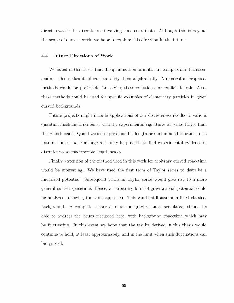
direct towards the discreteness involving time coordinate. Although this is beyond
the scope of current work, we hope to explore this direction in the future.
4.4 Future Directions of Work
We noted in this thesis that the quantization formulas are complex and transcen-
dental. This makes it difficult to study them algebraically. Numerical or graphical
methods would be preferable for solving these equations for explicit length. Also,
these methods could be used for specific examples of elementary particles in given
curved backgrounds.
Future projects might include applications of our discreteness results to various
quantum mechanical systems, with the experimental signatures at scales larger than
the Planck scale. Quantization expressions for length are unbounded functions of a
natural number n. For large n, it may be possible to find experimental evidence of
discreteness at macroscopic length scales.
Finally, extension of the method used in this work for arbitrary curved spacetime
would be interesting. We have used the first term of Taylor series to describe a
linearized potential. Subsequent terms in Taylor series would give rise to a more
general curved spacetime. Hence, an arbitrary form of gravitational potential could
be analyzed following the same approach. This would still assume a fixed classical
background. A complete theory of quantum gravity, once formulated, should be
able to address the issues discussed here, with background spacetime which may
be fluctuating. In this event we hope that the results derived in this thesis would
continue to hold, at least approximately, and in the limit when such fluctuations can
be ignored.
69
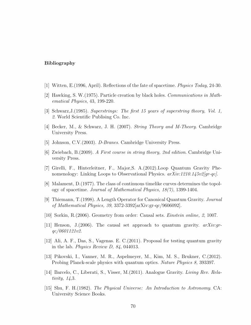
Bibliography
[1] Witten, E.(1996, April). Reflections of the fate of spacetime. Physics Today, 24-30.
[2] Hawking, S. W.(1975). Particle creation by black holes. Communications in Math-ematical Physics, 43, 199-220.
[3] Schwarz,J.(1985). Superstrings: The first 15 years of superstring theory, Vol. 1,2. World Scientific Publising Co. Inc.
[4] Becker, M., & Schwarz, J. H. (2007). String Theory and M-Theory. CambridgeUniversity Press.
[5] Johnson, C.V.(2003). D-Branes. Cambridge University Press.
[6] Zwiebach, B.(2009). A First course in string theory, 2nd edition. Cambridge Uni-versity Press.
[7] Girelli, F., Hinterleitner, F., Major,S. A.(2012).Loop Quantum Gravity Phe-nomenology: Linking Loops to Observational Physics. arXiv:1210.145v2[gr-qc].
[8] Malament, D.(1977). The class of continuous timelike curves determines the topol-ogy of spacetime. Journal of Mathematical Physics, 18(7), 1399-1404.
[9] Thiemann, T.(1998). A Length Operator for Canonical Quantum Gravity. Journalof Mathematical Physics, 39, 3372-3392[arXiv:gr-qc/9606092].
[10] Sorkin, R.(2006). Geometry from order: Causal sets. Einstein online, 2, 1007.
[11] Henson, J.(2006). The causal set approach to quantum gravity. arXiv:gr-qc/0601121v2.
[12] Ali, A. F., Das, S., Vagenas. E. C.(2011). Proposal for testing quantum gravityin the lab. Physics Review D, 84, 044013.
[13] Pikovski, I., Vanner, M. R., Aspelmeyer, M., Kim, M. S., Brukner, C.(2012).Probing Planck-scale physics with quantum optics. Nature Physics 8, 393397.
[14] Barcelo, C., Liberati, S., Visser, M.(2011). Analogue Gravity. Living Rev. Rela-tivity, 14,3.
[15] Shu, F. H.(1982). The Physical Universe: An Introduction to Astronomy. CA:University Science Books.
70
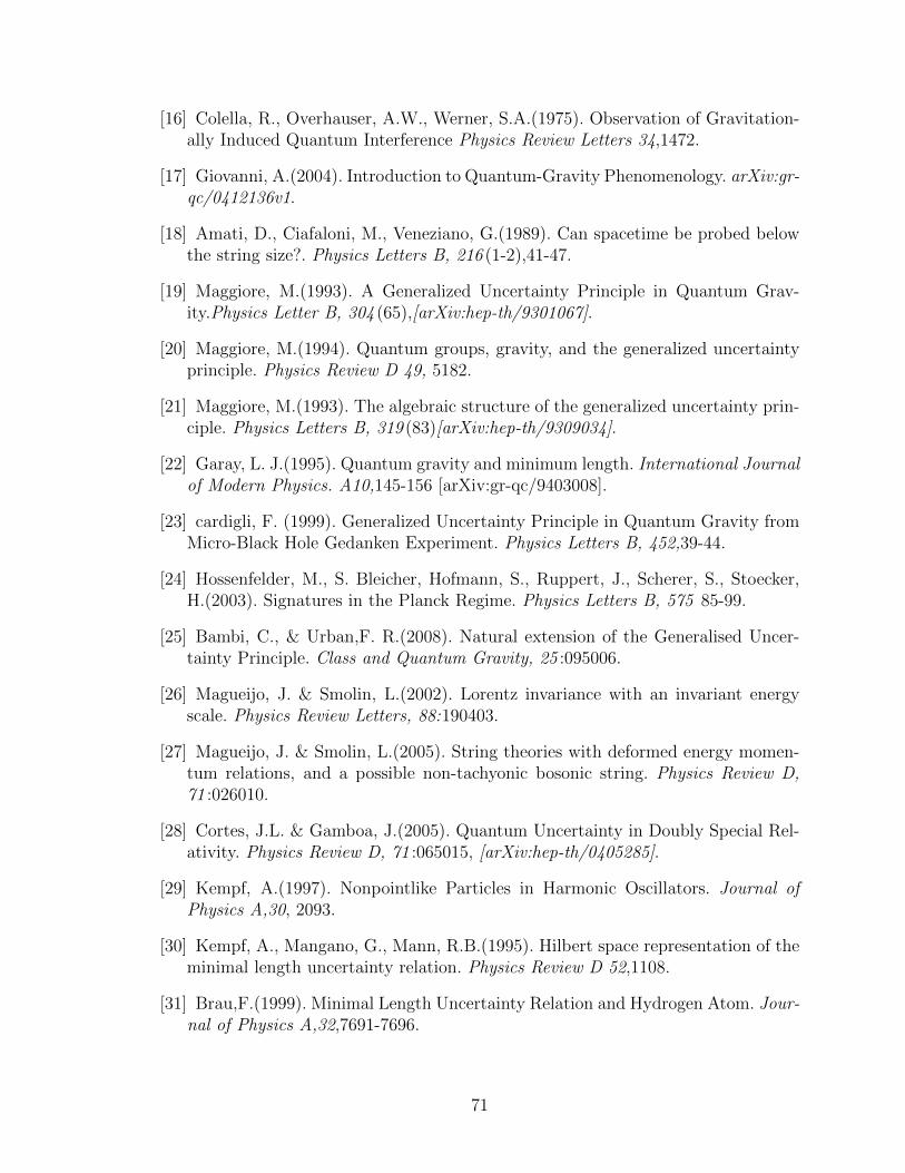
[16] Colella, R., Overhauser, A.W., Werner, S.A.(1975). Observation of Gravitation-ally Induced Quantum Interference Physics Review Letters 34,1472.
[17] Giovanni, A.(2004). Introduction to Quantum-Gravity Phenomenology. arXiv:gr-qc/0412136v1.
[18] Amati, D., Ciafaloni, M., Veneziano, G.(1989). Can spacetime be probed belowthe string size?. Physics Letters B, 216 (1-2),41-47.
[19] Maggiore, M.(1993). A Generalized Uncertainty Principle in Quantum Grav-ity.Physics Letter B, 304 (65),[arXiv:hep-th/9301067].
[20] Maggiore, M.(1994). Quantum groups, gravity, and the generalized uncertaintyprinciple. Physics Review D 49, 5182.
[21] Maggiore, M.(1993). The algebraic structure of the generalized uncertainty prin-ciple. Physics Letters B, 319 (83)[arXiv:hep-th/9309034].
[22] Garay, L. J.(1995). Quantum gravity and minimum length. International Journalof Modern Physics. A10,145-156 [arXiv:gr-qc/9403008].
[23] cardigli, F. (1999). Generalized Uncertainty Principle in Quantum Gravity fromMicro-Black Hole Gedanken Experiment. Physics Letters B, 452,39-44.
[24] Hossenfelder, M., S. Bleicher, Hofmann, S., Ruppert, J., Scherer, S., Stoecker,H.(2003). Signatures in the Planck Regime. Physics Letters B, 575 85-99.
[25] Bambi, C., & Urban,F. R.(2008). Natural extension of the Generalised Uncer-tainty Principle. Class and Quantum Gravity, 25 :095006.
[26] Magueijo, J. & Smolin, L.(2002). Lorentz invariance with an invariant energyscale. Physics Review Letters, 88:190403.
[27] Magueijo, J. & Smolin, L.(2005). String theories with deformed energy momen-tum relations, and a possible non-tachyonic bosonic string. Physics Review D,71 :026010.
[28] Cortes, J.L. & Gamboa, J.(2005). Quantum Uncertainty in Doubly Special Rel-ativity. Physics Review D, 71 :065015, [arXiv:hep-th/0405285].
[29] Kempf, A.(1997). Nonpointlike Particles in Harmonic Oscillators. Journal ofPhysics A,30, 2093.
[30] Kempf, A., Mangano, G., Mann, R.B.(1995). Hilbert space representation of theminimal length uncertainty relation. Physics Review D 52,1108.
[31] Brau,F.(1999). Minimal Length Uncertainty Relation and Hydrogen Atom. Jour-nal of Physics A,32,7691-7696.
71
[32] Ali, A.F., Das, S., Vagenas, E.(2009). Discreteness of space from the generalizeduncertainty principle. Physics Letters B, 678 (5),497-499.
[33] Ali, A.F., Das, S., Vagenas, E.(2010). Discreteness of Space from GUP II: Rela-tivistic Wave Equations. Physics Letters B, 690 (4), 407-412.
[34] Landau, L. D., & Lifschitz, E. M.(1991). Quantum Mechanics (Non-RelativisticTheory), 3rd edition. Oxford, England:Pergamon Press.
[35] Polyanin, A.D., & Zeitsev, V.F.(2003). Handbook of Exact Solutions for OrdinaryDifferential Equations. Chapman and Hall.
[36] Das, A.(2008). Lectures in Quantum Mechanics. Singapore: World ScientificPublishing.
[37] Bologna, M.(2005). Short Introduction to Fractional Calculus. Universidad deTarapaca, Arica, Chile. Lecture Notes, 41-54.
[38] Cohen-Tannoudji, C., Diu, B., Laloe, F.(1991).Quantum Mechanics, vol. 1.Wiley-VC.
[39] Dirac, P. A. M.(1928). The quantum theory of the electron. Proceedings of theRoyal Society A: Mathematics, Physics and Engineering Science 117 (778): 610.
[40] Alberto, P., Fiolhais, C., Gil, V. M.(1996). Relativistic particle in a box. Euro-pean Journal of Physics, 17, 19-24.
[41] Chodos, A., Thorn,C.B.(1974). Electromagnetic self-energy of confined masslessquarks. Physics Letters B, 53 (4), 359-361.
72

Appendices
73

Appendix A
Dimensions and Relative Magnitudes
[~] = m2kgs−1
k = mkgs−2
µ = m−1
α = `Pl/~
k2m2x2
µ6α2~6=
(mkgs−2)2(kg)2m2
(m−1)6(`Pl/~)2(m2kgs−1)6= 1
km
µ3~2
(1 + µα~)
µ2α2~2
µα~ = m−1(`Pl/~)~ = 1
km
µ3~2=
(mkgs−2)kg
(m−3)(m2kgs−1)2= 1
ε can be considered as having the dimension of 1/k.
74
~ ∼ 10−34m2kgs−1
`Pl ∼ 10−35m
m ∼ 10−30kg
x ∼ 10`Pl
(1)E ∼ 10−30 × (3× 108)2 ≈ 10−30+17 ≈ 10−13kgm2s−2 (rest energy of an electron)
(2)k2m2x2
µ6α2~6∼ k2
10−30×2 × 100l2pl × 10−2×34
8× 10−30×3 × 10−13×3`2Pl
≈ k2 10−60−68+2+90+39
8≈ 10−4k2
(3)k2m2
µ6~4
((1 + µα~)
µ2α2~2
)2
µα~ ∼√
2mE
~2
`Pl~~ ≈√
2× 10−30 × 10−13 × 1034 × 10−35 ≈ 10−22.5 ≈ 10−23
k2m2
µ6~4
((1 + µα~)
µ2α2~2
)2
∼ k210−30×2 × 10−34×2
8× 10−30×3 × 10−13×3
(1 + 10−23
10−23×2
)2
≈ 1090+39−60−68+92
8≈ 1094k2
(4)2k2m
µ3~2
((1 + µα~)
µ2α2~2
)≈ k210−30 × 10−34
23/2 × 10−30× 32 × 10−13× 3
2
(1 + 10−23
10−23×2
)≈ 1045k2
(5)2k2mx
µ3α~3∼ k210−30 × 10`Pl × 10−34
23/2 × 10−30×2× 32 × 10−13× 3
2 × `Pl≈ k2 2
23/210−64+1+45+19.1 ≈ k2.
(A.1)
75
Appendix B
Dimension Check for k and Comparison with α
k2 <<µ6α2~6
m2x2
dim
[µ6α2~6
m2x2
]=
(1m
)6 ( `Pl~
)2 ~6
kg2m2
=m2~4
kg2m8
=m2(m2kgs−1)4
kg2m8
=m10kg2s−4
m8
=m4kg2s−4
m2
[k] =m2kgs−2
m[Energy
length
]=m(kg(ms2
))m
.
The underlying assumption of the perturbative approach is that the perturbationmust be very small compared to the unperturbed wavefunction, i.e., kψ1 < ψ0∣∣∣∣kψ1
ψ0
∣∣∣∣2 = ε2k2 +k2m2x2
µ6α2~6+k2m2
µ6~4
((1 + µα~)
µ2α2~2
)2
+2εk2m
µ3~2
((1 + µα~)
µ2α2~2
))− 2εk2mx
µ3α~3.
The term with the highest order of magnitude is k2m2
µ6~4
((1+µα~)µ2α2~2
)2
. Setting this as
<< 1 we get
k2 <<µ6~4
m2
(µ2α2~2
(1 + µα~)
)2
≈ 10−94
⇒ k << 10−47.
76
Taking x ∼ 10`Pl, (α ∼ α0`Pl
~≈ 1× 10⁻³⁵
10−34≈ 10−1 = 0.1
).
This means k can be considered as smaller than α.
77

Appendix C
Derivatives
C.1 Computation of some useful quantities
ψ0(E, k.x) = C1Ai(−ξ) + C2Bi(−ξ)
=C1√πξ−1/4 sin
(2
3ξ
32 +
π
4
)+C2√πξ−1/4 cos
(2
3ξ
32 +
π
4
)(C.1)
= C1ψI0 + C2ψ
II0 ,
where ξ =(
2m~2) 1
3 k−23 (E − kx).
dξ
dx=
(2m
~2
) 13
k−23 (−k) = −
(2m
~2
) 13
k13 (C.2)
dξ
dE=
(2m
~2
) 13
k−23 (C.3)
dψ20
dx2=
d
dx
(dψ0
dξ
dξ
dx
)=
d
dx
(dψ0
dξ
)dξ
dx+dψ0
dξ
d
dx
(dξ
dx
)=
d
dξ
(dψ0
dξ
)dξ
dx
dξ
dx+ 0
=
(dξ
dx
)2d
dξ
(dψ0
dξ
)⇒ d3ψ0
dx3=
d
dx
((dξ
dx
)2d2ψ0
dξ2
)=
(dξ
dx
)3d3ψ0
dξ3(C.4)
dψ0
dE=dψ0
dξ
dξ
dE(C.5)
.
78
d
dx
(dψ0
dE
)=
d
dx
(dψ0
dξ
dξ
dE
)=
d
dx
(dψ0
dξ
)dξ
dE+dψ0
dξ
d
dx
(dξ
dE
)=
d
dξ
(dψ0
dξ
)dξ
dx
dξ
dE+ 0
=d2ψ0
dξ2
dξ
dx
dξ
dE
⇒ d2
dx2
(dψ0
dE
)=
d
dx
(d
dx
dψ0
dE
)=
d
dx
(d2ψ0
dξ2
dξ
dx
dξ
dE
)=
d
dx
(d2ψ0
dξ2
)dξ
dx
dξ
dE+d2ψ2
0
dξ2
d
dx(dξ
dx)dξ
dE+d2ψ2
0
dξ2
dξ
dx
d
dx
(dξ
dE
)=
d
dξ
(d2ψ0
dξ2
)(dξ
dx
)2dξ
dE+ 0 + 0
=d3ψ0
dξ3
(dξ
dx
)2dξ
dE(C.6)
d3
dx3
(dψ0
dE
)=
d
dx
(d2
dx2
(dψ0
dE
))=
d
dx
(d3ψ0
dξ3
(dξ
dx
)2dξ
dE
)
=d
dx
(d3ψ0
dξ3
)(dξ
dx
)2dξ
dE+ 0 + 0
=d
dξ
(d3ψ0
dξ3
)(dξ
dx
)3dξ
dE
=d4ψ0
dξ4
(dξ
dx
)3dξ
dE(C.7)
79
C.2 Calculation of derivatives required in sec 2.3.1
1.dψ0
dξ= C1
dψI0dξ
+ C2dψII0
dξ
=C1√π
[−1
4ξ−5/4 sin
(2
3ξ3/2 +
π
4
)+ ξ1/4 cos
(2
3ξ3/2 +
π
4
)]+
C2√π
[−ξ1/4 sin
(2
3ξ3/2 +
π
4
)− 1
4ξ−5/4 cos
(2
3ξ3/2 +
π
4
)].
2.d2ψ0
dξ2=
C1√π
[−1
4
(−5
4
)ξ−
54−1 sin
(2
3ξ3/2 +
π
4
)−
1
4ξ−
54+
12 cos
(2
3ξ3/2 +
π
4
)+
1
4ξ
14−1 cos
(2
3ξ3/2 +
π
4
)− ξ 1
4+12 sin
(2
3ξ3/2 +
π
4
)]+
C2√π
[−1
4ξ
14−1 sin
(2
3ξ3/2 +
π
4
)− ξ 1
4+12 cos
(2
3ξ3/2 +
π
4
)− 1
4
(−5
4
)ξ−
54−1 cos
(2
3ξ3/2 +
π
4
)+
1
4ξ−
54+
12 sin
(2
3ξ3/2 +
π
4
)]=
C1√π
[5
16ξ−9/4 sin
(2
3ξ3/2 +
π
4
)− 1
4ξ−3/4 cos
(2
3ξ3/2 +
π
4
)+
1
4ξ−3/4 cos
(2
3ξ3/2 +
π
4
)−
ξ3/4 sin
(2
3ξ3/2 +
π
4
)]+C2√π
[−1
4ξ−3/4 sin
(2
3ξ3/2 +
π
4
)− ξ3/4 cos
(2
3ξ3/2 +
π
4
)+
3
16ξ−9/4 cos
(2
3ξ3/2 +
π
4
)+
1
4ξ−3/4 sin
(2
3ξ3/2 +
π
4
)]
(C.8)
=C1√π
[5
16ξ−9/4 sin
(2
3ξ3/2 +
π
4
)− ξ3/4 sin
(2
3ξ3/2 +
π
4
)]+C2√π
[−ξ3/4 cos
(2
3ξ3/2 +
π
4
)]= − C1√
π
[ξ3/4 sin
(2
3ξ3/2 +
π
4
)]− C2√
π
[ξ3/4 cos
(2
3ξ3/2 +
π
4
)](C.9)
3.d3ψ0
dξ3= − C1√
π
[3
4ξ
34−1 sin
(2
3ξ3/2 +
π
4
)+ ξ
34
+ 12 cos
(2
3ξ3/2 +
π
4
)]−
C2√π
[3
4ξ
34−1 cos
(2
3ξ3/2 +
π
4
)− ξ
34
+ 12 sin
(2
3ξ3/2 +
π
4
)]= − C1√
π
[3
4ξ−1/4 sin
(2
3ξ3/2 +
π
4
)+ ξ5/4 cos
(2
3ξ3/2 +
π
4
)]+
C2√π
[−3
4ξ−1/4 cos
(2
3ξ3/2 +
π
4
)+ ξ5/4 sin
(2
3ξ3/2 +
π
4
)]
80
4.d4ψ0
dξ4=
C1√π
[(3
16ξ−5/4 + ξ7/4
)sin
(2
3ξ3/2 +
π
4
)− 2ξ1/4 cos
(2
3ξ3/2 +
π
4
)]+
C2√π
[(3
16ξ−5/4 + ξ7/4
)cos
(2
3ξ3/2 +
π
4
)+ 2ξ1/4 cos
(2
3ξ3/2 +
π
4
)](C.10)
81