aspects of twistors and tractors in field theory

Aspects of twistors and tractors in field

theory

Jack Williams

Department of Applied Maths and Theoretical Physics

University of Cambridge

This dissertation is submitted for the degree of

Doctor of Philosophy

Clare College April 2021

Declaration

I hereby declare that except where specific reference is made to the work of others, the

contents of this dissertation are original and have not been submitted in whole or in part

for consideration for any other degree or qualification in this, or any other university.

This dissertation is my own work and contains nothing which is the outcome of work

done in collaboration with others, except as specified in the text and Acknowledgements.

This dissertation contains fewer than 65,000 words including appendices, bibliography,

footnotes, tables and equations and has fewer than 150 figures.

Jack Williams

April 2021

Acknowledgements

I am extremely grateful to my supervisor David Skinner for his support and guidance

throughout the past four years. His inexhaustible supply of ideas, guided by extraordinary

intuitive understanding of physics, has been a constant source of inspiration for our work

together. I want to thank him particularly for the generosity he has shown me with his

time, and for spending more than a few long evenings puzzling over a blackboard.

Early in my PhD, I had the pleasure of collaborating with Tim Adamo, whose sense of

humour enlivened even the longest and most laborious calculations. His patience and

willingness to explain things in simple terms made for a smooth start to my PhD.

My officemates, Roland, Antoni, Carl and James have provided much needed, and

occasionally mathematical, distractions as well as moral support and cake. Long lunches

have been excellent respite, and I would like to thank Alice, Charles, Chris, Giuseppe,

Julija, Manda, Nathan, Roxana and Toby in particular. Outside of physics, I feel fortunate

to have the friendship of many kind and supportive people. I am especially thankful to

Sarah, Anna, Pavel, Megan, Jesse, Adrien, Ellie and Johanna. Most of all, I would like to

express my gratitude to Jess, who was by my side through the arduous route to this thesis,

especially the latter stages.

Finally, I am grateful for my family, for their immense support and encouragement at

every step.

Abstract

This thesis is divided into three sections.

The first begins with a review of the Fefferman-Graham embedding space construction

and the closely-related tractor calculus, which provides a simple way to catalogue and

invent conformally invariant operators. In particular, the conformal wave operator arises

as the descendant of the ordinary wave operator on the Fefferman-Graham space. We

construct a worldline action on the Fefferman-Graham space whose equations of motion

descend to a conformally coupled scalar on the base manifold. We present also a novel

Fefferman-Graham worldline action for the massless Dirac equation and demonstrate

that it descents to a Dirac spinor on the base manifold. Unlike the scalar, the massless

Dirac equation is conformally invariant without modification.

The second concerns the application of twistor theory to five-dimensional anti-de

Sitter space. The twistor space of AdS5 is the same as the ambitwistor space of the four-

dimensional conformal boundary; the geometry of this correspondence is reviewed for

both the bulk and boundary. A Penrose transform allows us to describe free bulk fields,

with or without mass, in terms of data on twistor space. Explicit representatives for

the bulk-to-boundary propagators of scalars and spinors are constructed, along with

twistor action functionals for the free theories. Evaluating these twistor actions on bulk-

to-boundary propagators is shown to produce the correct two-point functions.

In the final chapter, we construct a minitwistor action for Yang–Mills–Higgs theory

in three dimensions. The Feynman diagrams of this action will construct perturbation

theory around solutions of the Bogomolny equations in much the same way that MHV

diagrams describe perturbation theory around the self–dual Yang Mills equations in four

dimensions. We also provide a new formula for all tree amplitudes in YMH theory (and its

maximally supersymmetric extension) in terms of degree d maps to minitwistor space.

We demonstrate its relationship to the RSVW formula in four dimensions and show that it

generates the correct MHV amplitudes at d = 1 and factorizes correctly in all channels for

all degrees.

Table of contents

1 Background 1

1.1 Twistor space for flat Minkowski spacetime . . . . . . . . . . . . . . . . . . . . 2

1.2 The Penrose transform for flat Minkowski spacetime . . . . . . . . . . . . . . 3

1.3 Summary of thesis . . . . . . . . . . . . . . . . . . . . . . . . . . . . . . . . . . 4

1.3.1 Twistors for conformally invariant theories . . . . . . . . . . . . . . . . 4

1.3.2 Twistors and the AdS/CFT correspondence . . . . . . . . . . . . . . . . 5

1.3.3 Twistors for amplitudes in quantum field theory . . . . . . . . . . . . 6

2 Tractors for conformal worldline theories 9

2.1 Introduction . . . . . . . . . . . . . . . . . . . . . . . . . . . . . . . . . . . . . . 9

2.2 Conformal geometry . . . . . . . . . . . . . . . . . . . . . . . . . . . . . . . . . 10

2.2.1 The conformal sphere as a lightcone inside R1,n+1 . . . . . . . . . . . . 10

2.2.2 Homogeneous functions on M as functions on N . . . . . . . . . . . 11

2.2.3 The tractor bundle . . . . . . . . . . . . . . . . . . . . . . . . . . . . . . 12

2.2.4 The tractor connection . . . . . . . . . . . . . . . . . . . . . . . . . . . . 12

2.2.5 The general ambient space construction . . . . . . . . . . . . . . . . . 15

2.3 Worldline scalar actions . . . . . . . . . . . . . . . . . . . . . . . . . . . . . . . 17

2.3.1 The conformally flat case . . . . . . . . . . . . . . . . . . . . . . . . . . 17

2.3.2 The general curved case . . . . . . . . . . . . . . . . . . . . . . . . . . . 19

2.4 Worldline Dirac actions . . . . . . . . . . . . . . . . . . . . . . . . . . . . . . . 21

2.4.1 The conformally flat case . . . . . . . . . . . . . . . . . . . . . . . . . . 21

2.4.2 The general curved case . . . . . . . . . . . . . . . . . . . . . . . . . . . 23

2.5 Discussion . . . . . . . . . . . . . . . . . . . . . . . . . . . . . . . . . . . . . . . 25

2.5.1 Obstructions . . . . . . . . . . . . . . . . . . . . . . . . . . . . . . . . . . 25

3 Twistor methods for AdS5 27

3.1 Introduction . . . . . . . . . . . . . . . . . . . . . . . . . . . . . . . . . . . . . . 27

3.2 Geometry . . . . . . . . . . . . . . . . . . . . . . . . . . . . . . . . . . . . . . . . 28

x Table of contents

3.2.1 AdS5 geometry from projective space . . . . . . . . . . . . . . . . . . . 28

3.2.2 The twistor space of AdS5 . . . . . . . . . . . . . . . . . . . . . . . . . . 32

3.3 The Penrose transform . . . . . . . . . . . . . . . . . . . . . . . . . . . . . . . . 37

3.3.1 Scalars: Direct and indirect transform . . . . . . . . . . . . . . . . . . . 38

3.3.2 Spinors: direct and indirect transform . . . . . . . . . . . . . . . . . . . 40

3.4 Free theory, Bulk-to-boundary propagators & 2-point functions . . . . . . . 42

3.4.1 Scalars . . . . . . . . . . . . . . . . . . . . . . . . . . . . . . . . . . . . . 42

3.4.2 Fundamental solution to the AdS wave equation . . . . . . . . . . . . 47

3.4.3 Spinors . . . . . . . . . . . . . . . . . . . . . . . . . . . . . . . . . . . . . 48

3.5 Discussion . . . . . . . . . . . . . . . . . . . . . . . . . . . . . . . . . . . . . . . 51

4 Minitwistors and 3d Yang-Mills-Higgs theory 53

4.1 Introduction . . . . . . . . . . . . . . . . . . . . . . . . . . . . . . . . . . . . . . 53

4.2 Minitwistor Theory . . . . . . . . . . . . . . . . . . . . . . . . . . . . . . . . . . 56

4.2.1 Geometry of minitwistor space . . . . . . . . . . . . . . . . . . . . . . . 56

4.2.2 Penrose transform & Hitchin-Ward correspondence . . . . . . . . . . 60

4.3 The Minitwistor Action . . . . . . . . . . . . . . . . . . . . . . . . . . . . . . . . 62

4.3.1 Action and equations of motion . . . . . . . . . . . . . . . . . . . . . . 62

4.3.2 Equivalence to space-time action . . . . . . . . . . . . . . . . . . . . . 68

4.3.3 Other Reality Conditions . . . . . . . . . . . . . . . . . . . . . . . . . . 72

4.4 Tree Amplitudes in YMH3 Theory . . . . . . . . . . . . . . . . . . . . . . . . . 73

4.4.1 A connected prescription generating functional . . . . . . . . . . . . . 74

4.4.2 Relation to the RSVW formula . . . . . . . . . . . . . . . . . . . . . . . 82

4.5 Discussion . . . . . . . . . . . . . . . . . . . . . . . . . . . . . . . . . . . . . . . 84

References 87

Appendix A AdS Laplacian and Dirac equation in embedding space coordinates 95

Chapter 1

Background

The causal structure of spacetime is of fundamental importance to physics. Information

cannot propagate between points which are spacelike-separated, whereas an adventurous

observer may travel between any two timelike-separated points. It is this fact which allows

us to do physics at all: experiments conducted on Earth can remain free of interference

from distant events unseen to the experimentalist, however extreme they may be.

Central to the causal structure of spacetime are null cones, which divide space into

three regions: those in our timelike past, from which we can receive information, those in

our timelike future, which can be influenced by our actions, and those outside our light

cone, with which we cannot interact. Even more fundamental are null vectors, which

show the directions along which light rays can travel away from a particular point. The

set of directions in which null rays can travel away from a source is indexed by S2, one for

each point in the sky. A more sophisticated way to see this is to view the 3-dimensional

light cone in R1,3 as a bundle over S2 whose fibres are the null generators. The Lorentz

action of SO(1,3) on Minkowski space preserves the lightcone and descends to an action

on the space of null rays through the origin, and hence also to a group action on S2.

One can ask how the positions of stars in the sky move under a Lorentz boost applied

to the Earth. It is easily checked that while the stars do move, the cross ratio of any set

of four holomorphic positions on S2 is an invariant. Cross ratios are preserved only by

Möbius transformations, so this must be the effect of a boost on the set of null directions.

This is the key insight: the celestial sphere S2 can be given a unique complex structure

and identified as the Riemann sphere. Relativity reveals a natural complex structure in the

sky invisible to the Galilean observer.

2 Background

1.1 Twistor space for flat Minkowski spacetime

This introduction to twistor theory summarises well-known work; see for example [85, 63,

110, 12].

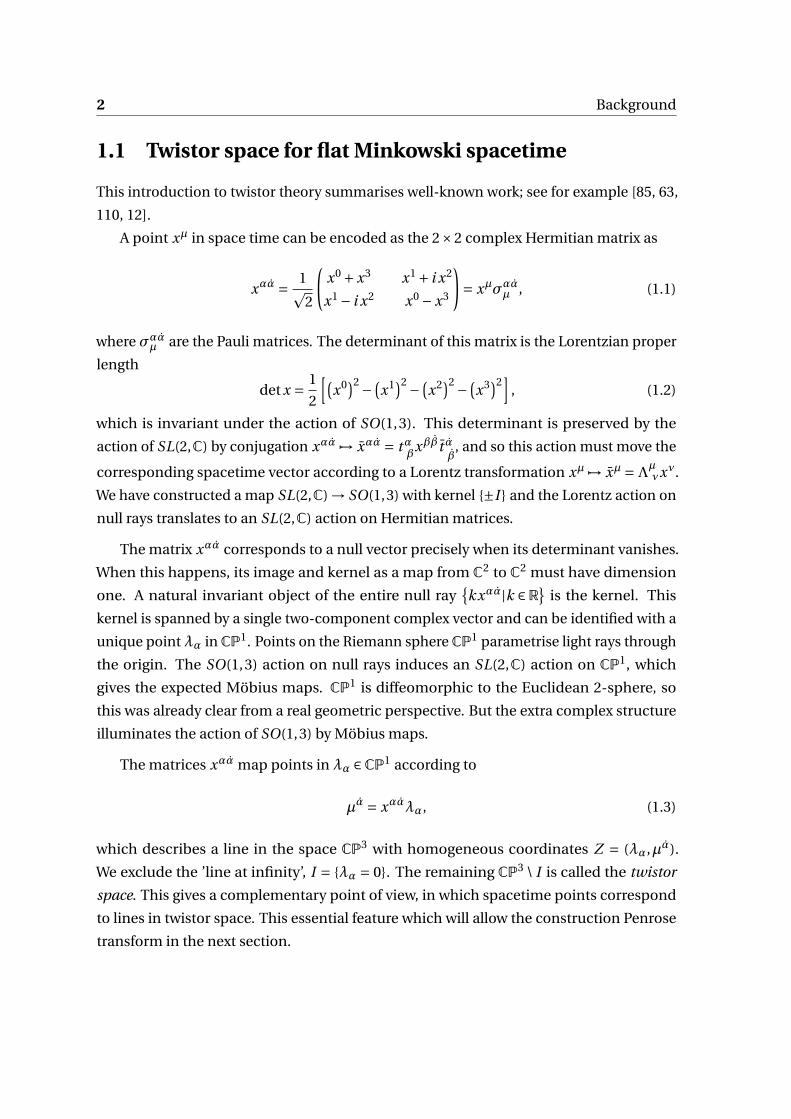
A point xµ in space time can be encoded as the 2×2 complex Hermitian matrix as

xαα = 1p2

(x0 +x3 x1 + i x2

x1 − i x2 x0 −x3

)= xµσααµ , (1.1)

where σααµ are the Pauli matrices. The determinant of this matrix is the Lorentzian proper

length

det x = 1

2

[(x0)2 − (

x1)2 − (x2)2 − (

x3)2]

, (1.2)

which is invariant under the action of SO(1,3). This determinant is preserved by the

action of SL(2,C) by conjugation xαα 7→ xαα = tαβ

xββ t αβ

, and so this action must move the

corresponding spacetime vector according to a Lorentz transformation xµ 7→ xµ =Λµνxν.

We have constructed a map SL(2,C) → SO(1,3) with kernel ±I and the Lorentz action on

null rays translates to an SL(2,C) action on Hermitian matrices.

The matrix xαα corresponds to a null vector precisely when its determinant vanishes.

When this happens, its image and kernel as a map from C2 to C2 must have dimension

one. A natural invariant object of the entire null raykxαα|k ∈R

is the kernel. This

kernel is spanned by a single two-component complex vector and can be identified with a

unique point λα in CP1. Points on the Riemann sphere CP1 parametrise light rays through

the origin. The SO(1,3) action on null rays induces an SL(2,C) action on CP1, which

gives the expected Möbius maps. CP1 is diffeomorphic to the Euclidean 2-sphere, so

this was already clear from a real geometric perspective. But the extra complex structure

illuminates the action of SO(1,3) by Möbius maps.

The matrices xαα map points in λα ∈CP1 according to

µα = xααλα, (1.3)

which describes a line in the space CP3 with homogeneous coordinates Z = (λα,µα).

We exclude the ’line at infinity’, I = λα = 0. The remaining CP3 \ I is called the twistor

space. This gives a complementary point of view, in which spacetime points correspond

to lines in twistor space. This essential feature which will allow the construction Penrose

transform in the next section.

1.2 The Penrose transform for flat Minkowski spacetime 3

From the perspective of null rays, one can fix a point Z = (λα,µα) in twistor space an

ask which spacetime points correspond to lines passing through that point. If µα = 0, we

already know the answer: x must lie on the null ray through the origin corresponding to

λα. If µα = 0, then if we can find one solution to equation (1.3), all others must differ from

it by points whose kernel is λα. Again, we obtain a null ray, but offset from the origin.

This gives a point-line duality: points in spacetime correspond to holomorphic lines

in twistor space. The λα components hold information about the direction of our null

ray, and the µα components hold information about the location of the ray relative to the

origin.

1.2 The Penrose transform for flat Minkowski spacetime

The wave equation is one of the simplest and most important partial differential equations.

In this section, we explain how its solutions can be represented by functions on twistor

space, and describe the Penrose transform as a map between physical solutions and

twistorial representatives.

Given a (0,1)-form f (λ,µ) on the twistor space of complexified Minkowski spaceCP3\I ,

one can construct a function φ :R1,3 →C on spacetime in a canonical way

φ(x) =∫

Lx

f (λ,µ)⟨λdλ⟩, (1.4)

where Lx is the line in twistor space corresponding to spacetime point x and ⟨λdλ⟩ is the

projective measure ϵαβλαdλβ. The 1-form f (λ,µ) must have homogeneity -2 so that the

integral is well defined. In practice, the integral over Lx means setting µα = xααλα and

performing the integral over λ. This is the Penrose transform. It can be seen to satisfy the

spacetime wave equation,

φ(x) = ϵαβϵαβ∂αα∂ββφ(x) (1.5)

= ϵαβϵαβ∂αα∂ββ∫

Lx

f (λα, xααλα)⟨λdλ⟩ (1.6)

= ϵαβϵαβ∫

Lx

λαλβ∂

∂µα∂

∂µβf (λα, xααλα)⟨λdλ⟩ (1.7)

= 0, (1.8)

provided f depends on the twistor variables only holomorphically (∂ f = 0). Moreover, any

solution to the wave equation can be obtained this way [48].

4 Background

It is easy to see that the Green’s function, φ = 1(x−y)2 , can be written as a Penrose

transform. Two twistor points A,B determine a twistor line, and hence a spacetime point

y . A simple integration shows that the Penrose representative

f (Z ) = 1

A ·Z∂

(1

B ·Z

)(1.9)

reproduces the Green’s function on spacetime.

The map between solutions and their Penrose representatives is not one-to-one. In-

deed, any ∂-exact form may be added to a Penrose representative f 7→ f + ∂g without

changing the value of the integral. Representatives which differ by exact derivatives should

be regarded as equivalent, and the map is really between cohomology classes of ∂, ∂-closed

forms on twistor space modulo ∂-exact forms. We will also use Penrose transforms for

fields of other spin throughout this thesis. Particles of spin s are represented by elements

of the cohomology class H 0,1(CP3 \ I ,O (−2s −2)

)[83, 48].

1.3 Summary of thesis

Twistor theory has been highly successful for tackling problems of classical geometry.

The utility of the Penrose transform to reformulate not just linear problems, such as

the wave equation, but also non-linear ones, such as the self-dual Yang-Mills equations

and self-dual gravity, in terms of simpler, unconstrained problems on twistor space is

among its most important achievements. Solutions to complicated geometric problems

in spacetime are exchanged for holomorphic functions in twistor space.

It is natural to ask whether this classical geometric success of twistor theory can be

matched by applications in quantum field theory.

1.3.1 Twistors for conformally invariant theories

The ambient metric construction of Fefferman and Graham [51, 56] is a powerful tool for

studying conformal geometry. It allows one to build, from a given n dimensional manifold

M , a manifold M of dimension n +2 which depends only on the conformal class of the

metric on M , and not on the particular representative. The manifold M and all objects

constructed from it are necessarily conformal invariants, meaning that they are preserved

by Weyl transformations of the metric g 7→ Ω2g . A null cone inside M contains as its

sections embeddings of M and all conformally related manifolds.

1.3 Summary of thesis 5

The metric on M is chosen to be Ricci flat by solving a recurrence relation order-by-

order in a parameter in a direction off the cone. Whether this construction is possible

depends of the vanishing of a certain obstruction tensor, which in four dimensions is the

conformally invariant Bach tensor.

The primary motivation for this construction was to discover and classify conformally

invariant tensors beyond a handful which were already known such as the Weyl tensor and

the Bach tensor. This aim was achieved [51, 50]. Among the conformal tensors discovered

are the various obstruction tensors arising in the construction of the Fefferman-Graham

ambient metric.

Our purpose for the ambient construction is different. In chapter 1, we describe a

worldline quantum mechanical theory whose target space is the Fefferman-Graham space

for a given base manifold M . In doing so, we ensure that the theory we construct is

conformally invariant. By imposing constraints, we reduce the Hilbert space to lower

dimensional one and the theory descends to a conformally invariant one on M . In general,

one encounters ordering ambiguities when quantising quantum theories, but we demon-

strate that no such ambiguities arise in our theory on M by virtue of its construction from

the ambient space.

Our goal is to understand quantum fields in the presence of general conformal cur-

vature. We consider both a scalar, which descends to a conformally coupled scalar, and

a Dirac spinor, which descends to a ordinary Dirac spinor on M . Both these descended

theories are conformally invariant as desired. We do so first in the simple case of a confor-

mally flat base manifold, whose ambient space is flat Minkowski space, but then are able

to generalise to the case of conformal curvature without significant additional conceptual

difficulty.

The Fefferman-Graham construction has also found applications in the study of the

AdS/CFT correspondence. AdS space of dimension n +1 is viewed as the projectivisation

of the Fefferman-Graham embedding space of dimension n, and asymptotically AdS

spaces can be constructed from fluctuations on the conformal boundary [94].

1.3.2 Twistors and the AdS/CFT correspondence

The holographic principle has its origins in black hole thermodynamics. While the entropy

of most systems grows as the cube of its length scale, a black hole’s grows only quadrati-

cally in its radius, proportional to the area of its event horizon. This suggests that the only

degrees of freedom are on the surface, and can be encoded in a space of one fewer dimen-

sion that the space in which the black hole lives. More recently, Maldacena conjectured a

6 Background

duality between type IIB string on AdS5 ×S5 space, and the conformal field theory N = 4

super Yang-Mills on its conformal boundary [73, 114]. Much evidence has been found

in favour of this conjecture (e.g [39]), and it is widely expected to be true. Nonetheless,

many important questions remain unanswered. Self-dual N = 4 super Yang-Mills is a

simplification of the well-known example which retains the conformal invariance of the

original. This theory should be dual to a simpler string theory in the bulk, providing a

simpler example of an AdS/CFT correspondence than is currently available. One might

hope that this setting would permit a more secure understanding of the correspondence

than is possible in the full duality of N = 4 super-Yang-Mills.

In this thesis, we look only at the basic steps of finding twistor representatives for scalar

and spinor bulk-to-boundary propagators, which will be crucial in any further study of

the subject. By writing some of the ingredients of the AdS/CFT correspondence in twistor

space, one might hope to find a theory on twistor space which generates the observables.

In chapter 3, we describe the twistor space of AdS5 and construct explicit twistor

representatives for scalar and spinor bulk-to-boundary propagators, some of the most

fundamental objects in the correspondence, and verify that a natural twistor action for

these fields reproduces the expected form of the two-point boundary correlation function.

1.3.3 Twistors for amplitudes in quantum field theory

A major success of twistor theory is the RSVW formula [115, 89] for all tree amplitudes

in N = 4 super-Yang-Mills theory in four dimensions. The amplitudes generated by

this functional are organised around the self–dual sector, and indexed by a parameter d

grading the NMHV degree of the scattered particles.

∞∑d=0

g 2d(4)

∫dµ(d)

Clogdet(∂+A4)|C (1.10)

where the integral is taken over all degree d holomorphic maps Z : CP1 → CP3|4 from

a rational curve to N = 4 twistor space CP3|4. Expanding in powers of the on-shell

background field A4, this formula is a generating functional for all tree amplitudes in

N = 4 SYM4. Each of the elements of this formula will be explained in the context of three-

dimensional Yang-Mills-Higgs theory in chapter 3. The compactness of this generating

functional, compared with other methods of calculation, such as the Feynman diagram

expansion, is its most impressive feature.

The proof that this functional produces the correct amplitudes proceeds by check-

ing first that it produces the correct 3-point functions, and then that the residues of its

1.3 Summary of thesis 7

poles factorise correctly, so that it satisfies the BCFW recursion relations expected of an

amplitude [103, 95, 25, 24].

In chapter 3, we present a dimensional reduction of this theory, the three dimensional

Yang-Mills-Higgs theory, and offer an analogous formula for the full set of tree-level

amplitudes. We demonstrate its correctness by calculating 3-point functions and checking

the factorisation property.

Chapter 2

Tractors for conformal worldline

theories

2.1 Introduction

This section begins with an introduction to the conformal geometry required to construct

a conformal worldline quantum mechanical model. The conformally flat sphere is the

simplest case and is discussed first, before generalising to the general case of conformal

curvature and arbitrary topology. The basic idea, described in [51], is to construct from our

base manifold (M , g ) a higher dimensional spacetime (M ,G ) by adding one spacelike and

one timelike direction. The higher dimensional spacetime depends only on the conformal

class of the base metric g , though this fact will not be manifest, and inside it lies a null cone

N whose sections (not necessarily planar) are embeddings of (M , g ) and all spacetimes

which can be obtained from (M , g ) by Weyl rescalings of the metric. The direction along

the null generators of the cone corresponds to Weyl rescaling.

In the simple case of a conformally flat base, the ambient space is flat R1,n+1 and the

embeddings of spacetimes conformally equivalent to the sphere arise as sections of the

light cone at the origin. The ‘horizontal section’ obtained by intersection with a horizontal

plane induces a round sphere, while the parabolic section induces flat Rn . Hyperbolic

space arises from hyperbolic sections of the cone.

On restriction to these ‘conic sections’, operators on the ambient space descend to

operators on the base manifold. Given that the ambient space depends only on the

conformal class of the base manifold, these operators must be conformal invariants.

We consider actions for worldline quantum mechanical theories in the ambient space.

By imposing natural constraints, we restrict these theories to the cone and a homogeneity

10 Tractors for conformal worldline theories

along the null generators of the cone, which corresponds to conformal weight of various

fields. We treat only the massless scalar and Dirac spinor, but other possibilities exist. The

massless free scalar action descends to a scalar on the base whose equation of motion is

the conformal wave equation. Since the massless Dirac equation is conformally invariant,

we find the descendent of a massless Dirac spinor in the ambient space to be a massless

Dirac spinor on the base.

Ambiguities typically arise in the quantisation of quantum mechanical worldline

theories. For example, ordering ambiguities may arise in the Laplacian or in other natural

operator expressions. One solution, is to impose a particular renormalisation scheme. We

will see that important properties of the ambient space construction allow us to avoid

these problems and construct a worldline action in a natural and conformally invariant

manner.

2.2 Conformal geometry

2.2.1 The conformal sphere as a lightcone inside R1,n+1

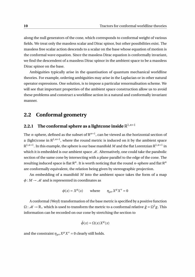
The n-sphere, defined as the subset of Rn+1, can be viewed as the horizontal section of

a (light)cone in R1,n+1, where the round metric is induced on it by the ambient space

R1,n+1. In this example, the sphere is our base manifold M and the flat LorentzianR1,n+1 in

which it is embedded is our ambient space M . Alternatively, one could take the parabolic

section of the same cone by intersecting with a plane parallel to the edge of the cone. The

resulting induced space is flat Rn . It is worth noticing that the round n-sphere and flat Rn

are conformally equivalent, the relation being given by stereographic projection.

An embedding of a manifold M into the ambient space takes the form of a map

φ : M →M and is represented in coordinates as

φ(x) = X µ(x) where ηµνX µX ν = 0

A conformal (Weyl) transformation of the base metric is specified by a positive function

Ω : M →R+ which is used to transform the metric to a conformal relative g =Ω2g . This

information can be recorded on our cone by stretching the section to

φ(x) =Ω(x)X µ(x)

and the constraint ηµνX µX ν = 0 clearly still holds.

2.2 Conformal geometry 11

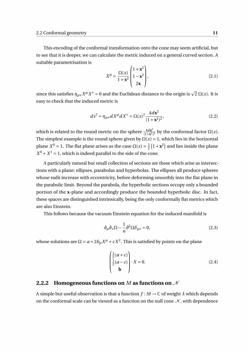
This encoding of the conformal transformation onto the cone may seem artificial, but

to see that it is deeper, we can calculate the metric induced on a general curved section. A

suitable parametrisation is

X µ = Ω(x)

1+x2

1+x2

1−x2

2x

, (2.1)

since this satisfies ηµνX µX ν = 0 and the Euclidean distance to the origin isp

2Ω(x). It is

easy to check that the induced metric is

d s2 = ηµνd X µd X ν =Ω(x)2 4dx2

(1+x2)2, (2.2)

which is related to the round metric on the sphere 4dx2

(1+x2)2 by the conformal factor Ω(x).

The simplest example is the round sphere given byΩ(x) = 1, which lies in the horizontal

plane X 0 = 1. The flat plane arises as the caseΩ(x) = 12

(1+x2

)and lies inside the plane

X 0 +X 1 = 1, which is indeed parallel to the side of the cone.

A particularly natural but small collection of sections are those which arise as intersec-

tions with a plane: ellipses, parabolas and hyperbolas. The ellipses all produce spheres

whose radii increase with eccentricity, before deforming smoothly into the flat plane in

the parabolic limit. Beyond the parabola, the hyperbolic sections occupy only a bounded

portion of the x-plane and accordingly produce the bounded hyperbolic disc. In fact,

these spaces are distinguished intrinsically, being the only conformally flat metrics which

are also Einstein.

This follows because the vacuum Einstein equation for the induced manifold is

∂µ∂νΩ− 1

n∂2Ωδµν = 0, (2.3)

whose solutions areΩ= a +2bµX µ+ c X 2. This is satisfied by points on the plane12 (a + c)12 (a − c)

b

·X = 0. (2.4)

2.2.2 Homogeneous functions on M as functions on N

A simple but useful observation is that a function f : M →C of weight λ which depends

on the conformal scale can be viewed as a function on the null cone N , with dependence


on the scale replaced by dependence on the position along the null generator of the

cone. In particular, a homogeneous function f : M → C can be viewed as a function

with homogeneity in X , since scaling X is equivalent to sliding up the side of the cone.

Homogeneity of weight λ translates to the condition X ·∂ f =λ f .

2.2.3 The tractor bundle

One of the early motivations for the tractor bundle construction was to proliferate and

systematically catalogue conformal invariants beyond the few that were already known –

the Weyl tensor and the Bach tensor [97]. The idea is to take a vector field in the ambient

space M which is restricted (but not necessarily tangent) to the null cone N and is

conformally invariant, or homogeneous of degree zero.

A tractor will be defined to be a vector field which is homogeneous of degree zero

and parallel transported along a single null generator of the cone ([38], following [98–

100]). The vector belongs to the tangent space to the entire ambient space M and may

have components pointing off the cone. A tractor field consists of a tractor on each null

generator of the cone and descends to a field on the base manifold M . It is clear that

the space of tractors at a point in M is a vector space and so the tangent space to the

ambient manifold descends to a vector bundle over M , the tractor bundle T . Tractor

fields are sections of the tractor bundle. We will not discuss the construction of conformal

invariants using tractors, but details are given in [38].

More important for the present discussion will be the connection induced on the

tractor bundle by the ambient space and the question of the existence of flat sections. In

this example it is clear that we have n +2 independent flat sections which descend from

flat vector fields on Rn+2. This fact may not hold in the general case. In fact, we will see

that the existence of a flat section of the tractor bundle is equivalent to the existence of an

Einstein section of the cone.

2.2.4 The tractor connection

As a first step towards constructing the ambient space for a general base manifold and

metric, we give an intrinsic description of the tractor connection on T . There are two

main advantages of this intrinsic construction. The first is that dependence on only the

conformal class of the base metric is manifest. The second is that it makes clear why

parallel sections of T correspond to Einstein metrics in the class. This section closely

follows the presentation of [38].


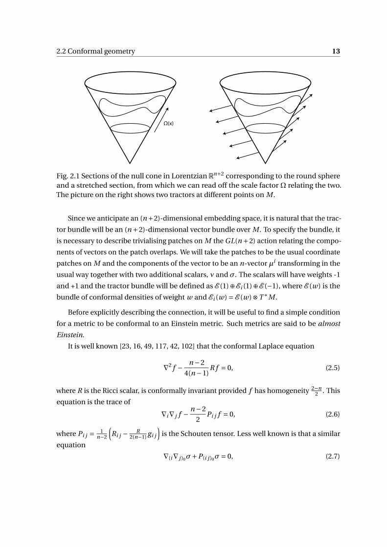
Ω(x)

Fig. 2.1 Sections of the null cone in Lorentzian Rn+2 corresponding to the round sphereand a stretched section, from which we can read off the scale factor Ω relating the two.The picture on the right shows two tractors at different points on M .

Since we anticipate an (n+2)-dimensional embedding space, it is natural that the trac-

tor bundle will be an (n +2)-dimensional vector bundle over M . To specify the bundle, it

is necessary to describe trivialising patches on M the GL(n +2) action relating the compo-

nents of vectors on the patch overlaps. We will take the patches to be the usual coordinate

patches on M and the components of the vector to be an n-vector µi transforming in the

usual way together with two additional scalars, ν and σ. The scalars will have weights -1

and +1 and the tractor bundle will be defined as E (1)⊕Ei (1)⊕E (−1), where E (w) is the

bundle of conformal densities of weight w and Ei (w) = E (w)⊗T ∗M .

Before explicitly describing the connection, it will be useful to find a simple condition

for a metric to be conformal to an Einstein metric. Such metrics are said to be almost

Einstein.

It is well known [23, 16, 49, 117, 42, 102] that the conformal Laplace equation

∇2 f − n −2

4(n −1)R f = 0, (2.5)

where R is the Ricci scalar, is conformally invariant provided f has homogeneity 2−n2 . This

equation is the trace of

∇i∇ j f − n −2

2Pi j f = 0, (2.6)

where Pi j = 1n−2

(Ri j − R

2(n−1) gi j

)is the Schouten tensor. Less well known is that a similar

equation

∇(i∇ j )0σ+P(i j )0σ= 0, (2.7)


where T(i j )0 denotes the symmetric traceless part of Ti j , is conformally invariant provided

σ has homogeneity 1 [13]. The traceless part of the Schouten tensor is proportional to the

traceless part of the Ricci (and hence Einstein) tensor. If gi j is Einstein, this must vanish

and the equation reduces to ∇(i∇ j )0σ= 0, which is evidently satisfied by σ= 1. If we make

a conformal transformation from an Einstein metric toΩ2gi j , then σ transforms to σ=Ωand (2.7) continues to hold by conformal invariance.

Conversely, if we have a positive solution σ = Ω to (2.7), then we can perform the

inverse conformal transformation Ω−1. Under this transformation, σ transforms back

to σ= 1 and satisfies (2.7) with respect to the new metric. Since the first term vanishes,

the second must also and we learn that the traceless Schouten tensor vanishes. Since the

Schouten tensor is a trace-adjusted Ricci tensor, it follows that the traceless Ricci tensor

vanishes too and the new metric is Einstein. Therefore, the existence of an Einstein metric

in the conformal class is equivalent to the existence of a positive solution to (2.7). For this

reason, (2.7) is called the almost Einstein equation.

To understand this equation better, notice that solving the almost Einstein equation is

obviously equivalent to solving

∇i∇ jσ+Pi jσ−νgi j = 0.

If we set µi =∇iσ, then this is replaced by a system of two equations

∇iσ−µi = 0, (2.8)

∇iµ j +Pi jσ−νgi j = 0. (2.9)

A simple calculation shows that these imply a third equation,

∇iν−Pi jµj = 0, (2.10)

where µ j = g j iµi .

Now we are ready to see how flat sections of the tractor bundle correspond to Einstein

metrics. We simply define the tractor bundle to have components (ν,µi ,σ) and the tractor

connection to be

∇Ti

ν

µ j

σ

=

∇iν−Pi jµ

j

∇iµj +P j

i σ−νδ ji

∇iσ−µi

. (2.11)


From a parallel section of this connection, we can read off the conformal factorσ satisfying

the almost Einstein equation and, conversely, we can construct a flat section from a given

almost Einstein solution σ.

This definition of the tractor connection looks as though it depends on the conformal

factor. However, two tractor bundles constructed using two different, but conformally

equivalent, metrics are isomorphic. Suppose gi j is a fixed representative of a particular

conformal class. The isomorphism relating the bundle constructed using e2u(x)gi j to the

one constructed from e2u(x)gi j is given bye−uν

e uµi

e uσ

=

1 0 0

−∇i u δij 0

12 (∇u)2 −∇ j u 1

e−uν

euµ j

euσ

. (2.12)

It is important that the tractor connection be covariant with respect to this isomorphism

[38], a fact which can be checked directly but which will follow immediately once we see

how the connection arises from the ambient space construction.

2.2.5 The general ambient space construction

The crucial step is the generalisation of the ambient space construction to n-dimensional

base manifolds (M , g ) which are not conformally flat. A natural guess would be to start

with a cone whose horizontal sections are isometric to constant conformal scalings of

(M , g ), and then extend the metric off the cone such that the ambient metric is flat.

Unfortunately, this is not possible.

A more realistic suggestion is to ask that the ambient space be Ricci-flat. It can be

shown that such a metric must take the form

G =−2ρd t 2 −2td tdρ+ t 2gi j (x,ρ)d xi d x j , (2.13)

where gi j (x,0) = gi j (x) is the base metric and the higher order terms in ρ are chosen

order-by-order such that G is Ricci-flat [51]. This is always possible to order n2 in ρ, and

the remainder of the series is uniquely determined provided a certain obstruction tensor,

which will be described later vanishes. The cone is the surface ρ = 0 and t is a scaling

variable (the metric is homogeneous of degree 2 in t). The section of the cone t = 1 has

induced metric gi j (x) so this is where we find the embedding of our base manifold.


In the special case where gi j (x) = e2u(x)δi j is conformally flat, the function gi j (x,ρ)

terminates at quadratic order and we have [51, 47]

gi j (x,ρ) = gi j −2ρPi j +ρ2g kl Pi k P j l , (2.14)

where Pi j (x) is the Schouten tensor corresponding to gi j (x).

We expect this to reduce to the flat Rn+2 considered in the previous section, and upon

making the change of variables

X 0 = teu[

x2 +1

2+e−2uρ

(1

2(∇u)2 x2 +1

2+x ·∇u +1

)],

X 1 = teu[

x2 −1

2+e−2uρ

(1

2(∇u)2 x2 −1

2+x ·∇u +1

)],

X = teu[

x+e−2uρ

(1

2(∇u)2 x+∇u

)],

(2.15)

it is seen that the ambient metric is indeed flat. We discovered this change of variables by

finding the Killing forms of the Fefferman-Graham embedding space. Our parametrisation

of conic sections (2.1) is now simply a special case of this transformation with ρ = 0 and

t = 1 and yields the submanifold (M ,e2uδi j ), as expected. Another easy calculation finds

that X 2 =−2ρt 2 so ρ = 0 does describe the null cone.

Notice that in this case, the metric (2.13) appears to depend on gi j but is in fact flat for

all choices of scale u(x). Hence, the ambient space depends only on the conformal class

to which gi j belongs, in this case the class of conformally flat metrics.

The tractor connection is simply the Levi-Civita connection of the ambient space [38].

It is easy to explicitly recover the intrinsic definition (2.11) by restricting the components

of the connection to a particular section of cone ρ = 0, t = 1 corresponding to some choice

of conformal scale. Although the resulting bundle appears to depend on this section, we

saw earlier that different sections produce isomorphic bundles. How should bundles over

different sections be identified in the extrinsic picture?

In the conformally flat case, we defined a tractor at a point in M to be a vector field of

homogeneity zero along a null generator of the cone. This allows us to identify vectors

living at different sections of the cone (but on the same null ray) and hence to identify the

different tractor bundles. The isomorphism (2.12) gave an intrinsic relation between the

components of vectors in two bundles corresponding to two different sections.

We can now understand this isomorphism extrinsically. The components of corre-

sponding vectors in the coordinate basis inherited from the flat ambient coordinates

(2.15) should be equal. So we can transform the components of each vector to the flat

2.3 Worldline scalar actions 17

coordinate basis and equate them. This will give us a relation between the components of

vectors in the more natural bundle coordinates (ν,µi ,σ). Explicit calculation yields the

same matrix as (2.12).

Following this example in the general case, we define a tractor to be a vector field along

a generator of the cone which is parallel with respect to the ambient metric. This gives us

a bijection between bundles constructed from different sections: corresponding vectors

are obtained by parallel transport along null generators of the cone.

We have now constructed both the ambient space and tractor bundle in a way which

superficially used the base metric, but the result turned out to depend only on the confor-

mal class. These constructions will be useful for building a conformally invariant worldline

action.

2.3 Worldline scalar actions

When constructing worldline actions on the base manifold, the constraints such as P 2

must be quantised. Ordering ambiguities may be partially resolved by requiring that

the quantum operator be diffeomorphism invariant [18]. Under such a scheme, the

wave operator would take the form ∇2 +kR, where R is the Ricci curvature and k is an

undetermined constant. A particularly attractive choice of k would be − n−24(n−1) , so that the

wave operator becomes the conformal Laplacian (2.5), but such a choice is unmotivated.

The virtue of the Fefferman-Graham embedding space for constructing such actions is

that it is Ricci flat, so there is a canonical choice of diffeomorphism-invariant quantisation.

It is conformal, so we expect to obtain the conformal wave equation as the equation of

motion upon descent to the base manifold. We show this to be correct, and demonstrate

the wider applicability of actions descended from Fefferman-Graham space obtaining a

Dirac spinor, which is conformal, from a Dirac action on the embedding space.

Some similar work has been done on the bosonic, conformally flat case in [21] and

related papers.

2.3.1 The conformally flat case

The action for a free massless particle on the flat ambient Rn+2 can be written in Hamilto-

nian form

S[X ,P ] =∫ (

X ·P + α

2P 2

)d t , (2.16)

where α is a Lagrange multiplier [44]. Since we have seen that the null cone X 2 = 0

provides a model for the conformal geometry, we will restrict our model to the cone by


imposing this an additional constraint. For canonical quantisation by Dirac’s method

[45, 40], the constraints should be first-class so we are forced to add a third constraint1

2X 2,

1

2P 2

= 1

2(X ·P +P ·X ) = X ·P − i

n +2

2.

The whole action becomes

S[X ,P ] =∫ (

X ·P + α

2P 2 + β

2X 2 + γ

2(X ·P +P ·X )

)d t , (2.17)

We impose these constraints directly on the Schrödinger wavefunctionΨ(X ) [69, 91,

41]. The cone constraint X 2Ψ= 0 implies thatΨ takes the form

Ψ(X ) = δ(X 2)φ(X ). (2.18)

The scaling constraint(−i X ·∂− i n+2

2

)Ψ= 0 implies that

0 =(

X ·∂+ n +2

2

)δ(X 2)φ(X ) (2.19)

= 2X 2δ′(X 2)φ(X )+δ(X 2)X ·∂φ(X )+ n +2

2φ(X ) (2.20)

=−2δ(X 2)φ(X )+δ(X 2)X ·∂φ(X )+ n +2

2δ(X 2)φ(X ) (2.21)

= δ(X 2)

(X ·∂+ n −2

2

)φ(X ) (2.22)

and so φ has homogeneity 2−n2 . The final constraint ∂2Ψ= 0 descends to an equation on

each section of the cone

∇2φ− n −2

4(n −1)Rφ= 0, (2.23)

where R is the induced scalar curvature [38]. This will be shown directly in the next section

in the more general case of a conformally curved base manifold. Here, we have obtained

is the conformal Laplace equation (2.5) and φ has the correct homogeneity for conformal

invariance. We have therefore succeeded in building a conformally invariant theory on M .

This was to be expected because ∂ is the tractor connection on the ambient space, which

depends only on the conformal class of the base manifold.

In addition the constraint equations, we need an inner product to fully define the

Hilbert space. A natural Hermitian inner product on M is

⟨ f , g ⟩ =−i∫Σ

ph n j (

f ∇ j g − g∇ j f)

, (2.24)

2.3 Worldline scalar actions 19

where Σ⊂ M is a hypersurface, h is the induced metric and ni is a unit normal. This inner

product is a conformal invariant. Under a conformal transformation,

⟨ f , g ⟩ 7→−i∫ΣΩn−1

ph

(Ω−1n j

)((Ω

2−n2 f

)∇ j

(Ω

2−n2 g

)−

(Ω

2−n2 g

)∇ j

(Ω

2−n2 f

))(2.25)

=−i∫Σ

ph n j

(f ∇ j g + 2−n

nf g∂ j (logΩ)− g∇ j f − 2−n

nf g∂ j (logΩ)

)(2.26)

= ⟨ f , g ⟩ (2.27)

Applying Stokes’ theorem and using the conformal Laplace equation shows that this inner

product is independent of Σ. To complete the discussion of the conformally flat case, we

write this inner product in flat ambient coordinates

⟨ f , g ⟩ =−i∫Σ

(nyDn+1X

)δ(X 2)

n · ( f ∂g − g∂ f)

n2. (2.28)

Here, Dn+1X = ϵµ0µ1···µn+1 X µ0 d X µ1 · · ·d X µn+1 is the projective measure on the ambient

space and n is a lift of the normal ni to the tangent space of the cone. The lift is not

unique, so we will need to check that the resulting integrand is independent of the choice

of lift. Two different lifts are related by n = n +k X ·∂. The numerator n · ( f ∂g − g∂ f)

is

preserved because f and g have the same weight. The denominator is preserved because

n is tangent to the cone and X 2 = 0 on the support of the delta function. The measure is

preserved because the extra contribution is proportional to X ·∂y(X ·∂ydn+2X ) = 0.

2.3.2 The general curved case

It is now simple to generalise this worldline action to a general base manifold; the only

difficulty is finding the correct way to generalise the constraints. A key observation is

that the ambient metric (2.13) is quadratic in t , so the generator of dilations is t∂t . The

vector field X ·∂ generated dilations in the flat case so it is natural to try to identify these.

Ordering ambiguities arise when quantising P 2 = gµν(X )PµPν.

The constraints generalise to the curved case as follows. The X 2 constraint should be

interpreted not as a coordinate expression in the special case of a flat embedding space,

but as the metric length of the vector field generating scalings of this space. Since t is the

coordinate along the cone measuring scaling, this vector field should be X = t∂t . Hence,

1

2X 2 −→ 1

2(t∂)2 =−ρt 2. (2.29)


For the P 2 constraint, the usual prescription based on preserving diffeomorphism co-

variance yields −∇2 +αR since R is the only diffeomorphism invariant scalar quadratic

in derivatives [18]. Fortunately, we have a Ricci-flat ambient space, so this ambiguity is

irrelevant. From the Christoffel symbols,

Γti j = t

(−Pi j +ρ

(Pi k P k

j −1

n −4Bi j

)+O(ρ2)

)(2.30)

Γρtρ =

1

t(2.31)

Γρ

i j = gi j (2.32)

Γit j =

1

tδi

j (2.33)

Γiρ j =−P i

j −ρ(Pi k P k

j −1

n −4Bi j

)+O(ρ2) (2.34)

Γij k = Γi j +2ρ

(P i

l Γli j −

1

2P i l (

Pl j ,k + Plk, j − P j k,l s))

, (2.35)

where Pi j and Bi j are the lower dimensional Schouten and Bach tensors respectively, one

can calculate the scalar Laplacian

1

2P 2 −→−1

2∇2 =− 1

2t 2

(−2t∂t∂ρ+ (2−n)∂ρ+2ρ∂2

ρ−1

2(n −1)R(2ρ∂ρ− t∂t )+∇2

). (2.36)

The scaling constraint (X ·P +P ·X ) is properly quantised as the commutator of the two

other constraints. We have

1

2(X ·P +P ·X )φ(t ,ρ, x) −→

[−1

2∇2,−ρt 2

]φ(t ,ρ, x) (2.37)

=− 1

4t 2

(−4t 2 −4t 2ρ∂ρ−2t 3∂t + (2−n)t 2 +4ρt 2∂ρ(ρ)∂ρ)φ(t ,ρ, x)

(2.38)

=− 1

4t 2

(−4t 2 +4t 2 −2t 3∂t + (2−n)t 2 −4t 2)φ(t ,ρ, x) (2.39)

= 1

2

(t∂t + n +2

2

)φ(t ,ρ, x), (2.40)

which agrees with the commutator of the expressions (2.29) and (2.36) in Fefferman-

Graham coordinates. This operator continues to impose the right weight on the wavefunc-

tion, while the P 2 constraint still descends to the conformal Laplace equation on M when

2.4 Worldline Dirac actions 21

acting on wavefunctions of the form (2.18).

∇2(δ(ρt 2)t

2−n2 φ(x)

)=∇2

(δ(ρ)t−

n+22 φ(x)

)(2.41)

=− t−n+2

2

2t 2

(∇2 + (n −2)δ′(ρ)+ (2−n)δ′(ρ)

+ 1

2(n −1)R

(2ρδ′(ρ)+ n +2

2

))φ(x) (2.42)

= t−n+2

2 δ(ρt 2)

(∇2φ(x)− n −2

4(n −1)Rφ(x)

)(2.43)

In the curved case, the inner product (2.28) generalises straightforwardly.

⟨ f , g ⟩ =−i∫Σ

(nyDn+1X

)δ(X 2)

n · ( f ∂g − g∂ f)

n2(2.44)

7→ −i∫Σ

(t−1ny

(t∂tyt n+1pg d tdρd n x

))δ(ρt 2)

t−1n ·((

t2−n

2 f)∂(t

2−n2 g

)−

(t

2−n2 g

)∂(t

2−n2 f

))n2

(2.45)

=−i∫Σ

(ny

pg d n x

) n · ( f ∂g − g∂ f)

n2(2.46)

=−i∫Σ

ph

n · ( f ∂g − g∂ f)

n2, (2.47)

which agrees with the ordinary n-dimensional inner product given earlier.

2.4 Worldline Dirac actions

2.4.1 The conformally flat case

It is well known that quantising the four dimensional action

S[x, p] =∫ (

x ·p + iψ · ψ+ α

2p2

)(2.48)

produces a spinor. The x and p operators are quantised from Poisson brackets in the

usual way

xµ, pνP = δµν 7→ [xµ, pν] = iδµν (2.49)

while the fermionic constraints satisfy anticommutators

ψµ,ψνP = 2iηµν 7→ ψµ,ψν =−2ηµν. (2.50)


The fermionic operators are implemented by Dirac matrices γµ which satisfy these

anitcommutation relations. From them we can build raising and lowering operators,

γ1± = γ0 ±γ2 and γ2± = γ1 ± iγ3. We choose a ground state annihilated by γi−. There are

four independent components of the spinor obtained by acting with each of the γi+ at

most once. The (n+2)-dimensional Dirac matrices are built from the n-dimensional ones

using the Pauli matrices, γµ = (i I ⊗σ1, I ⊗σ2,γi ⊗σ3), and accordingly, the number of

components of the spinor doubles.

A simple way to supersymmetrise our Fefferman-Graham space action is to add a

fermion kinetic term and further constraints.

S[X ,P ] =∫ (

X ·P + iψ · ψ+ α

2P 2 + β

2X 2 + γ

2(X ·P +P ·X )+δX ·ψ+ϵP ·ψ

)d t . (2.51)

The anticommutation relation for ψ is given by ψµ,ψν =−2ηµν, so after quantisation ψµ

acts as a Dirac matrix Γµ. Accordingly, the wavefunction has a Dirac spinor index. The

multiplicative constraints X 2Ψ= 0 and (X ·Γ)Ψ= 0 imply that

Ψ(X ,ψ) = δ(X 2)(X ·Γ)φ(X ,ψ), (2.52)

since X ·Γ is a nilpotent operator on the support of the delta function. Moreover, its rank

is half the dimension of the representation space, so the constraint leaves half of the

components of the spinor wavefunction undetermined. This is sensible, because a Dirac

spinor in two fewer dimensions has half the degrees of freedom. We will later interpret

this condition as one which projects our ambient spinor to a spinor on the base.

The remaining condition Γ ·∂Ψ= /∂Ψ= 0 is the Dirac equation on the ambient space.

It restricts to a operator on the smaller spinor space described above because the Dirac

operator anticommutes with δ(X 2)(X ·Γ) provided φ has weight −n2 in X .

δ(X 2)(X ·Γ),Γ ·∂=−[

δ(X 2),Γ ·∂] (X ·Γ)+δ(X 2) X ·Γ,Γ ·∂ (2.53)

= 2X 2δ′(X 2)+2δ(X 2)(X ·∂)+δ(X 2)(n +2) (2.54)

= 2δ(X 2)(

X ·∂+ n

2

)(2.55)

Again, to define the Hilbert space we need to give a Hermitian inner product. A natural

inner product on M is

⟨Ψ1,Ψ2⟩ = i∫Σ

ph ψ1 /nψ2, (2.56)

2.4 Worldline Dirac actions 23

where as before n is a unit normal to Σ. This can again be written in flat ambient coordi-

nates

⟨Ψ1,Ψ2⟩ =−i∫Σ

(nyDn+1X

)δ(X 2)

Ψ1(X ·Γ)(n ·Γ)Ψ2 −Ψ2(X ·Γ)(n ·Γ)Ψ1

n2. (2.57)

The integrand is homogenous in both X and n. It is independent of the choice of lift on n

because making another choice n = n +X ·∂ adds a second (X ·Γ) factor to the numerator,

and on the support of δ(X 2), (X ·Γ)2 = −X 2 = 0. The inner product is clearly invariant

underΨ1 7→Ψ1 + (X ·Γ)χ but is also invariant underΨ2 7→Ψ2(X ·Γ)χ since n is tangent to

the cone.

2.4.2 The general curved case

The Dirac equation is invariant under a conformal transformation g 7→Ω2g provided the

Dirac spinor transforms as ψ 7→Ω− n−12 ψ. To see this, first note that the spin connection

transforms as

ωµνρ = 1

2

(eρa

(∂µea

ν −∂νeaµ

)−eµa

(∂νea

ρ −∂ρeaν

)+eνa

(∂ρea

µ−∂µeaρ

))7→Ω

(ωµνρ+ gµ[ν∂ρ] logΩ

).

(2.58)

So the Dirac operator transforms according to

/Dψ= γaeµa

(∂µψ+ 1

4γ[aγb]ω

abµ ψ

)7→Ω− n+1

2 γaeµa

(∂µψ+ 1

4γ[aγb]ω

abµ ψ− n −1

2∂µ(logΩ)ψ+ 1

2γ[bγc]e

bµecν∂ν(logΩ)ψ

)7→Ω− n+1

2 /Dψ.

(2.59)

Although the Laplacian is the square of the Dirac operator, it does not follow from this

(and is indeed untrue) that the plain Laplacian is conformally invariant because /Dψ is a

spinor of conformal weight −n+12 rather than −n−1

2 .

Writing the (n+2)-dimensional gamma matrices ΓA = (Γ1,Γ2,Γa) = (i I ⊗σ1, I ⊗σ2,γi ⊗σ3) in terms of the n-dimensional gamma matrices γi on the base manifold and the Pauli

matrices σi , we find that non-vanishing parts of the Fefferman-Graham spin connection


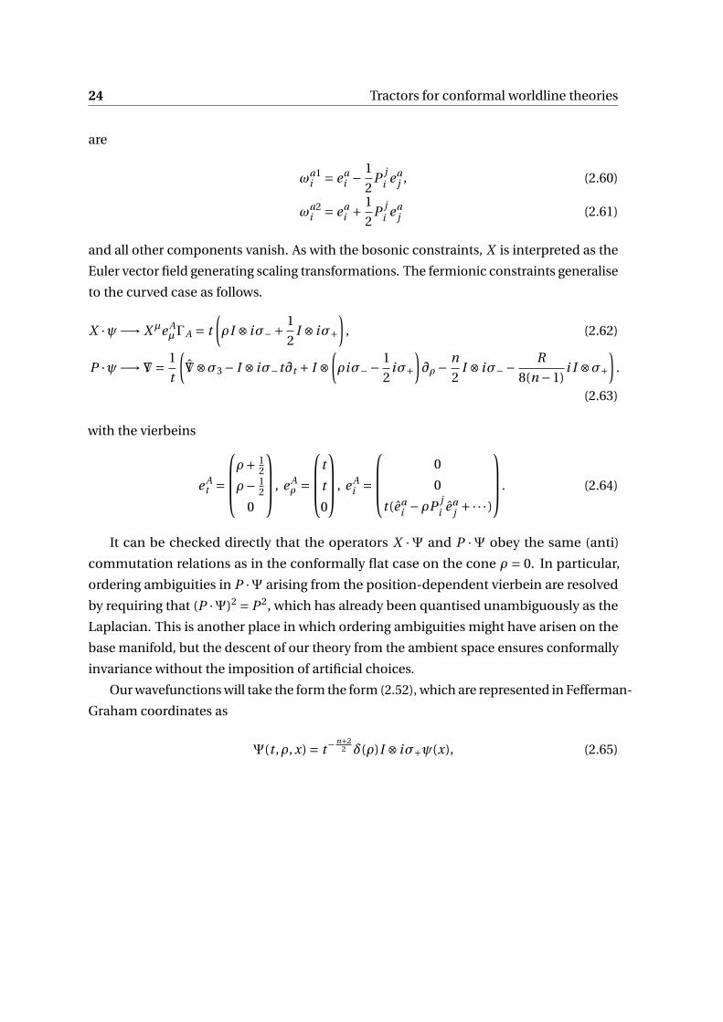
are

ωa1i = ea

i − 1

2P j

i eaj , (2.60)

ωa2i = ea

i + 1

2P j

i eaj (2.61)

and all other components vanish. As with the bosonic constraints, X is interpreted as the

Euler vector field generating scaling transformations. The fermionic constraints generalise

to the curved case as follows.

X ·ψ−→ X µe AµΓA = t

(ρI ⊗ iσ−+ 1

2I ⊗ iσ+

), (2.62)

P ·ψ−→ /∇= 1

t

(/∇⊗σ3 − I ⊗ iσ−t∂t + I ⊗

(ρiσ−− 1

2iσ+

)∂ρ− n

2I ⊗ iσ−− R

8(n −1)i I ⊗σ+

).

(2.63)

with the vierbeins

e At =

ρ+ 1

2

ρ− 12

0

, e Aρ =

t

t

0

, e Ai =

0

0

t (eai −ρP j

i eaj +·· · )

. (2.64)

It can be checked directly that the operators X ·Ψ and P ·Ψ obey the same (anti)

commutation relations as in the conformally flat case on the cone ρ = 0. In particular,

ordering ambiguities in P ·Ψ arising from the position-dependent vierbein are resolved

by requiring that (P ·Ψ)2 = P 2, which has already been quantised unambiguously as the

Laplacian. This is another place in which ordering ambiguities might have arisen on the

base manifold, but the descent of our theory from the ambient space ensures conformally

invariance without the imposition of artificial choices.

Our wavefunctions will take the form the form (2.52), which are represented in Fefferman-

Graham coordinates as

Ψ(t ,ρ, x) = t−n+2

2 δ(ρ)I ⊗ iσ+ψ(x), (2.65)

2.5 Discussion 25

where here we have the ρ terms vanish on the support of δ(ρt 2) = t−2δ(ρ). On such

wavefunctions, the operators X ·Ψ and P ·Ψ take the simplified forms

X ·ψ−→ 1

2t I ⊗ iσ+, (2.66)

P ·ψ−→ 1

t/∇⊗σ3, (2.67)

using ρδ′(ρ) =−δ(ρ), with all terms in ρ vanishing and the terms proportional to I ⊗σ+acting to give zero on the wavefunction.

The descended equation is therefore

δ(ρ) /∇⊗ iσ+ψ(x) = 0. (2.68)

Again, we interpret the σ+ factor as a projection onto the subspace of spinors which

originate on the base manifold. This is the Dirac equation on the base manifold.

2.5 Discussion

In this section, we have constructed worldline actions for the free massless scalar and

Dirac fermion on the Fefferman-Graham embedding space with constraints which allow

them to descend to theories on the base manifold. Since the Fefferman-Graham space

is conformally invariant, the descended theories are conformal. From the equations of

motion of these two theories, we obtain perhaps the two most famous and most important

conformal equations - the conformal wave equation and the Dirac equation. It seems

likely that other conformal theories, and their accompanying equations of motion, could

be obtained from the descent of other constrained theories defined on the Fefferman-

Graham space.

2.5.1 Obstructions

The ambient metric is constructed order-by-order in ρ so that the result is Ricci-flat. It

is shown in [51] that it is possible to all orders for odd n, and up to order n−22 for even n.

The existence and uniqueness of a solution beyond this depends on the vanishing of a

particular obstruction tensor. Naturally, this tensor is a conformal invariant, but explicit

formulae are difficult to obtain for all n. In the case n = 4, it is known to be the Bach tensor,

a classical conformal invariant given by

Bi j = Pkl W k li j +∇k∇i P j k −∇2Pi j . (2.69)


The Bach tensor is the metric variation of the 4 dimensional conformal anomaly∫M

Wabcd W abcdpg d 4x (2.70)

The construction of worldline actions depended on the vanishing of this obstruction,

but the conformal Laplace equation exists for any metric. This is because it uses the

Fefferman-Graham expansion only to low order.

It would be interesting to investigate connections between the obstruction tensor and

conformal anomalies.

Chapter 3

Twistor methods for AdS5

3.1 Introduction

In recent years, twistors have played an important role in studying scattering amplitudes

of four-dimensional gauge and gravitational theories. The fundamental tool underlying

these investigations is the (linear) Penrose transform [84, 48]. This asserts that solutions

to massless, free field equations on four-dimensional Minkowski space-time may be

described in terms of essentially arbitrary holomorphic functions on twistor space, with

the homogeneity of the function determining the helicity of the space-time field. The

asymptotic states in scattering processes are taken to obey such free field equations, so

twistors are a natural language in which to construct amplitudes.

Twistors also provide a natural arena in which to study four-dimensional CFTs. This

is because twistor space carries a natural action of SL(4,C), the (four-fold cover of the)

complexification of the space-time conformal group. Here, twistors are closely related to

the ‘embedding space’ formalism used in e.g. [43, 111, 82, 53, 81, 92, 37] and are particularly

useful when considering operators with non-integer spin [55, 52]. In the context of N = 4

SYM, twistor methods have been applied to correlation functions of local gauge invariant

operators in e.g. [4, 1, 33, 70, 34].

By the AdS/CFT correspondence, many four-dimensional CFTs have a dual description

as a theory of gravity in five-dimensional anti-de Sitter space [73, 57, 114]. Given the utility

of twistor theory on the boundary side of this correspondence, is natural to ask if it can

also be applied in the bulk.

In this chapter, we begin an investigation of the role of twistors in AdS5, following

earlier mathematical work in [14]. After briefly reviewing various descriptions of AdS and

its complexification, in section 3.2 we describe its twistor space and the corresponding

28 Twistor methods for AdS5

incidence relations. Remarkably, the twistor space of AdS5 turns out to be the same as the

ambitwistor space of the boundary space-time. We explore and elucidate this construction

in detail. In section 3.3 we consider the Penrose transform for free fields on AdS5. Unlike

in flat space-time, we show that it is straightforward to describe fields with non-zero mass

as well as non-zero spin. From the point of view of AdS/CFT, the most important free

fields are bulk-to-boundary propagators and we provide explicit twistor descriptions of

these in section 3.4, concentrating on spin-0 and spin- 12 . We also construct simple twistor

actions for these fields and verify that, when evaluated on bulk-to-boundary propagators,

they reproduce the expected form for 2-point correlation functions of boundary operators

of the expected conformal weights and spins. We hope that these results will provide a

useful starting-point for a twistor reformulation of Witten diagrams.

This chapter is based on collaborative work and primarily reproduced from [8].

3.2 Geometry

The geometry of anti-de Sitter space (or hyperbolic space) is an old and well-studied topic.

For the purposes of describing twistor theory in the context of five-dimensional AdS, a

particular description of hyperbolic geometry in terms of an open subset of projective

space will prove useful. While this description is standard, it is not often utilized in the

physics literature so we being with a brief review of AdS5 geometry from a projective point

of view. The twistor space of AdS5 and various aspects of its geometry are then discussed.

3.2.1 AdS5 geometry from projective space

Consider the five-dimensional complex projective space CP5, charted by homogeneous

coordinates encoded in a skew symmetric 4×4 matrix X AB = X [AB ] with the identification

X ∼λX for any λ ∈C∗. For a (holomorphic) metric written in terms of these homogeneous

coordinates to be well-defined on CP5 it must be invariant with respect to the scaling

X →λX and have no components along this scaling direction (i.e., the metric must not

‘point off’ CP5 into C6). The simplest metric satisfying these conditions is

ds2 =−dX 2

X 2+

(X ·dX

X 2

)2

, (3.1)

where skew pairs of indices are contracted with the Levi-Civita symbol, ϵABC D . This line

element is obviously scale invariant, and furthermore has no components in the scale

3.2 Geometry 29

direction. The latter fact follows since the contraction of (3.1) with the Euler vector field

Υ= X · ∂∂X vanishes.

Although this metric is projective (in the sense that it lives on CP5 rather than C6), it is

not global: (3.1) becomes singular on the quadric

M = X ∈CP5|X 2 = 0

⊂CP5 .

So (3.1) gives a well-defined metric on the open subset CP5 \ M . It is a fact that CP5 \

M equipped with this metric is equivalent to complexified AdS5, with the quadric M

corresponding to the four-dimensional conformal boundary. Real AdS5, along with a

choice of signature (Lorentzian or Euclidean, for instance) is specified by restricting the

metric to a particular real slice of CP5 – or equivalently, imposing some reality conditions

on X AB . We will be explicit about these reality conditions below.

To see that (3.1) really describes AdS5, it suffices to show that it is equivalent to other

well-known models of hyperbolic geometry. It is straightforward to see that the metric can

be rewritten as

ds2 =−ϵABC D d

(X AB

|X |)

d

(X C D

|X |)=−ϵABC D dX AB dX C D , (3.2)

where X AB := X AB /|X | with |X | :=p

X 2. The coordinates X AB are invariant under scal-

ings of X AB , so they give coordinates on C6 obeying X 2 = 1. Since (3.2) is just the flat

metric onC6, the original metric onCP5\M describes a geometry equivalent to the quadric

X 2 = 1 in C6. With an appropriate choice of reality conditions, this is the well-known

model of AdS5 as the hyperboloid in R6.

To obtain the conformal compactification of AdS5, one includes a conformal boundary

isometric to the one-point compactification of 4-dimensional complexified flat space; with

appropriate reality conditions this is topologically S4. We wish to identify this boundary

with the quadric M ⊂CP5 on which (3.1) becomes singular. A point X ∈ M satisfies X 2 = 0

and hence det X = 0. Since X AB is antisymmetric, non-zero and degenerate, it must have

rank 2 and so can be written as the skew of two 4-vectors,

X AB =C [ADB ] . (3.3)

However, X is projectively invariant under the (separate) transformations

(C ,D) 7→ (C ,D +αC ) , (C ,D) 7→ (C +βD,D) , (C ,D) 7→ (γC ,D) , (C ,D) 7→ (C ,δD)


I

Conformal Boundary

AdS Bulk

r

0

r ∞

P

X = P +1

2r2I

Surfaces of

constant r

Fig. 3.1 Parametrization of AdS space by Poincaré coordinates. The coordinate r controlsthe distance to the conformal boundary.

forα,β ∈C, γ,δ ∈C∗. Performing a sequence of these transformations allows us to assume

that C and D take the form

C =

a

c

1

0

and D =

b

d

0

1

, (3.4)

where some of a,b,c and d may be infinite, and after which there is no remaining freedom.

Thus, the general form of a boundary point is

X ABbdry =

(12 x2ϵαβ xαβ−xαβ ϵαβ

), (3.5)

where α, α, . . . are dotted and un-dotted two component SL(2,C) spinors. The four compo-

nents of xαα encode the four degrees of freedom in (3.4). Including the point ‘at infinity,’

represented by the infinity twistor

I AB =(ϵαβ 0

0 0

), (3.6)

gives the one-point compactification of four-dimensional flat space, with xαβ serving

as the usual spinor helicity coordinates. Thus, M = X 2 = 0 is identified with the S4

conformal boundary of AdS5. The relationship between four-dimensional space-time and

simple points in CP5 is well-established, having appeared in various places in a variety of

different guises (e.g., [43, 64, 111]).

3.2 Geometry 31

It is straightforward to obtain other well-known models of AdS5 from the projective

one. For example, the Klein model of hyperbolic space is obtained by simply writing

the metric (3.1) using inhomogeneous coordinates on a patch where one of the X AB is

non-vanishing. One of the models of AdS used most widely in physical applications is the

Poincaré model; in Euclidean signature these are global coordinates, and the metric takes

the form:

ds2 = dr 2 +dxααdxαα

r 2, (3.7)

with the conformal boundary corresponding to the region where r → 0.

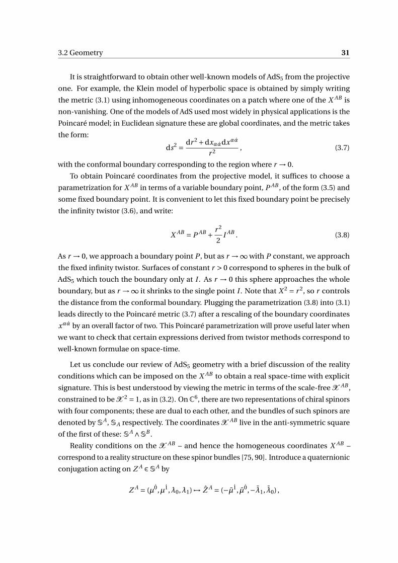
To obtain Poincaré coordinates from the projective model, it suffices to choose a

parametrization for X AB in terms of a variable boundary point, P AB , of the form (3.5) and

some fixed boundary point. It is convenient to let this fixed boundary point be precisely

the infinity twistor (3.6), and write:

X AB = P AB + r 2

2I AB . (3.8)

As r → 0, we approach a boundary point P , but as r →∞ with P constant, we approach

the fixed infinity twistor. Surfaces of constant r > 0 correspond to spheres in the bulk of

AdS5 which touch the boundary only at I . As r → 0 this sphere approaches the whole

boundary, but as r →∞ it shrinks to the single point I . Note that X 2 = r 2, so r controls

the distance from the conformal boundary. Plugging the parametrization (3.8) into (3.1)

leads directly to the Poincaré metric (3.7) after a rescaling of the boundary coordinates

xαα by an overall factor of two. This Poincaré parametrization will prove useful later when

we want to check that certain expressions derived from twistor methods correspond to

well-known formulae on space-time.

Let us conclude our review of AdS5 geometry with a brief discussion of the reality

conditions which can be imposed on the X AB to obtain a real space-time with explicit

signature. This is best understood by viewing the metric in terms of the scale-free X AB ,

constrained to be X 2 = 1, as in (3.2). OnC6, there are two representations of chiral spinors

with four components; these are dual to each other, and the bundles of such spinors are

denoted by SA, SA respectively. The coordinates X AB live in the anti-symmetric square

of the first of these: SA ∧SB .

Reality conditions on the X AB – and hence the homogeneous coordinates X AB –

correspond to a reality structure on these spinor bundles [75, 90]. Introduce a quaternionic

conjugation acting on Z A ∈SA by

Z A = (µ0,µ1,λ0,λ1) 7→ Z A = (−µ1, µ0,−λ1, λ0) ,


which squares to minus the identity: ˆZ A =−Z A. Clearly, there are no real spinors under

the · -operation, but this conjugation does act involutively on X AB . Restricting to the real

slice X AB = X AB inside C6 turns (3.2) into the flat metric on R1,5. This, along with the

condition that X 2 = 1 indicates that these reality conditions describe Euclidean AdS5 (the

hyperbolic spaceH5).

To obtain Lorentzian AdS5, a different reality condition is required. Instead of the

quaternionic conjugation, one can take ordinary complex conjugation which exchanges

the spinor representations:

Z A 7→ Z A = ZA .

The reality condition on X AB is then

X AB = XAB = 1

2ϵABC DX C D .

This real slice results in the flat metric on R2,4, and thus Lorentzian AdS5 as the hyper-

boloid.

3.2.2 The twistor space of AdS5

It is an interesting fact that the twistor space of AdS5 is the same geometric space as the

projective ambitwistor space of the complexified, four-dimensional conformal boundary.

In any number of dimensions, the projective ambitwistor space of a Riemannian manifold

MR is the space of complex null geodesics in the complexified manifold M [112, 66, 71,

113]. In the case that MR = S4, this ambitwistor space can be written as a quadric in

CP3 ×CP3:

Q = (Z A,WB ) ∈CP3 × (CP3)∗ |Z ·W = 0

, (3.9)

where Z A, WB are homogeneous coordinates on the two (dual) copies of CP3, each with

its own scaling freedom. The ambitwistor correspondence relates a point in M to a

CP1 × (CP1)∗ ⊂Q, which can be thought of as the complexified sphere of null directions

through that point.

The quadric Q also serves as the twistor space of (complexified) AdS5.1 The usual

twistor correspondence relates a space-time point to an extended geometric object in

twistor space, with the intersection theory of these objects encoding the conformal struc-

ture of the space-time. To formulate this correspondence, we relate AdS5 to Q by the

1This fact has been known for some time; a mathematical treatment was given by [14], and some aspectshave also appeared in the physics literature [88, 93, 11].

3.2 Geometry 33

incidence relations:

Z A = X AB WB , (3.10)

where X AB describes a point in AdS5. It is easy to see that for a fixed (up to scale) X , (3.10)

defines a CP3X ⊂ CP3 × (CP3)∗; the fact that CP3

X ⊂Q follows from the anti-symmetry of

X AB (i.e., the incidence relation preserves Z ·W = 0). Further, since X AB ∈CP5 \ M it has

no kernel so the incidence relation is non-degenerate.

For Q equipped with (3.10) to be the correct twistor space, the geometry of the inci-

dence relations should capture the conformal geometry of AdS5. To see this, consider two

distinct points X ,Y ∈CP5 \M and the correspondingCP3X ,CP3

Y ⊂Q. Generically, CP3X and

CP3Y will intersect in two projective lines in Q. To see this, note that CP3

X ∩CP3Y consists of

the points (Z ,W ) ∈CP3X for which (X − tY )AB WB = 0 for some t ∈C∗. The antisymmetric

matrix (X − tY )AB has a non-trivial kernel whenever it squares to zero, in which case its

kernel is of complex projective dimension one. This shows that CP3X ∩CP3

Y consists of

some number of copies of CP1. To establish how many, it is useful to write the intersection

condition in a scale-free way:

(X AB

|X | − sY AB

|Y |)

WB = 0 ⇔(

X

|X | − sY

|Y |)2

= 0.

This give a quadratic equation in s which has two distinct solutions given by

s± = X ·Y

|X ||Y | ±√(

X ·Y

|X ||Y |)2

−1, (3.11)

each of which corresponds to an intersection of CP3X ∩CP3

Y isomorphic to CP1.

Generically, these two lines do not themselves intersect because Y AB is non-degenerate.

However, whenX

|X | ·Y

|Y | = 1, (3.12)

these two solutions degenerate into a single CP1. Since the geodesic distance d(X ,Y )

between two points in AdS5 satisfies

cosh(d(X ,Y )) = X

|X | ·Y

|Y | , (3.13)

the pairs of points satisfying (3.12) are precisely those which are null separated. In other

words, two points in CP5 \ M are null separated in the AdS conformal structure if and only

if their corresponding CP3s intersect in a single line in twistor space.


( 3)* 3

X

X*

im X = ker X* = X

1

im X* = ker X = (X

1)*

Fig. 3.2 Relationship between the linear map X corresponding to a boundary point and itsdual. Both maps determine the canonical CP1 × (

CP1)∗

inside Q.

A null structure on a (complexified) Lorentzian manifold determines the metric up to

a conformal factor. The null structure given by this degeneracy condition is a canonical

choice, so we recover the AdS5 metric (3.1) up to the conformal factor. This factor is fixed

by making the canonical choice of holomorphic volume form on the CP3X corresponding

to a space-time point:

D3W := ϵABC DWAdWB ∧dWC ∧dWD , (3.14)

which sets the overall conformal factor in (3.1) to unity.

What happens in twistor space if X AB corresponds to a point on the conformal bound-

ary? This means that X 2 = 0 so X AB has a non-trivial kernel and the incidence relations

(3.10) become degenerate. In particular, since Z A are homogeneous coordinates on CP3,

they cannot all be simultaneously zero – but there are now solutions of X AB WB = 0. The

space of such solutions has complex projective dimension one, as does the image of X ABbdry

when viewed as a linear map on (CP3)∗. So for a boundary point Xbdry the degenerate

incidence relations are replaced by the linear map

Xbdry :(CP3)∗ \ (CP1

X )∗ →CP1X , (3.15)

where

(CP1X )∗ =

X AB

bdryWB = 0⊂ (CP3)∗ , CP1

X =

X bdryAB Z B = 0

⊂CP3 ,

are the kernel and image of the linear map, respectively.

In fact, boundary points Xbdry are in one-to-one correspondence with sets CP1X ×

(CP1X )∗ ⊂Q. The choice of CP1

X × (CP1X )∗ determines both the kernel and image of X AB

bdry,

and any antisymmetric 4×4 matrix is fixed by these up to an overall scale. This scale

is irrelevant because X AB describes a point in the projective space CP5. More generally,

3.2 Geometry 35

Z[ABB]

W ·B

Z[ABB]

W ·B

Fig. 3.3 The totally null set of points in spacetime CP5 corresponding to a twistor point(Z ,W ) for two different choices of B . We view B as fixed and vary A, tracing out a three-dimensional space of solutions. Changing B alters the parametrization of this solutionspace, but not the set itself.

any subset CP1X × (CP1

Y )∗ ⊂CP3 × (CP3)∗ can be specified by two points on the conformal

boundary xαα, yαα as in (3.5). The condition that this subset lies inside Q, namely that

Z ·W = 0 imposes the constraint xαα = yαα. Hence, the two lines CP1X × (CP1

Y )∗ ⊂ Q

correspond to the same point on the four-dimensional boundary.

This establishes the geometry of twistor space for both the bulk and boundary of AdS5.

A point in the bulk corresponds to aCP3 inside Q; for boundary points this correspondence

degenerates to give the standard ambitwistor relation between a point on the boundary

and a CP1 × (CP1)∗ inside Q.

It is equally natural to ask for the twistor correspondence in the other direction: what

does a point in twistor space correspond to in space-time? Given fixed (Z ,W ) ∈ Q, we

want to know which space-time points X satisfy the incidence relations

Z A = X AB WB .

The solution set consists of points of the form

X AB = Z [AB B ]

W ·B+ϵABC D AC WD , (3.16)

where AC is an arbitrary parameter and B B is an arbitrary twistor with B ·W = 0. Trans-

formations of the form A 7→ A+αW leave X invariant so the space of solutions is three-

dimensional. Making a different choice of B can be accommodated by a redefinition of A,

so B contributes no further degrees of freedom. Moreover, any tangent vector to this set is


Xbdry

Fig. 3.4 The set of points in spacetime CP5 corresponding to two different twistor points(Z ,W ) and (Z ,W ). The intersection is generically one-dimensional, but if Z ·W = 0 andZ ·W = 0, then it is two dimensional and the closure includes the boundary point whosecanonical CP1

X × (CP1

X

)∗ ⊂Q contains (Z ,W ) and (Z ,W ).

a null vector of the form ϵABC D (δA)C WD , where δA is a displacement in the parameter A.

Thus, a point in twistor space corresponds to a three-plane in CP5 and hence AdS5.

How can two such three-planes intersect? Let (Z ,W ), (Z ,W ) ∈Q be distinct twistor

points; the general projective solution to the simultaneous equations

Z A = X AB WB ,

Z A = X AB WB(3.17)

is

X AB =α(

Z [AB B ] Z ·WW ·B

− Z [AB B ] Z ·WW · B

+B [AB B ] (Z ·W )(Z ·W )

(B ·W )(B ·W )

)+γϵABC D WC WD , (3.18)

where α = 0 and B , B are such that B ·W = 0 and B ·W = 0 while B ·W = 0, B ·W = 0. This

solution is parametrized by the two complex numbers α,γ, or equivalently, a projective

line. So for all pairs (Z ,W ) and (Z ,W ) the corresponding null three-planes intersect in a

line in CP5.

3.3 The Penrose transform 37

However, if Z ·W = 0 and Z ·W = 0, then further solutions are possible. In this case,

the general solution is

X AB =αZ [AB B ]

W ·B+β Z [AB B ]

W · B+γϵABC D WC WD , (3.19)

with α,β = 0. This gives a two-dimensional projective space of solutions, parametrized

by homogeneous coordinates (α,β,γ). Note that the conditions Z ·W = 0 and Z ·W = 0

mean that (Z ,W ) and (Z ,W ) lie inside CP1X × (

CP1X

)∗ ⊂Q for a boundary point

X ABbdry = ϵABC D WC WD .

This point is in the closure of the two-dimensional intersection of their three-planes (3.19)

but not in the solution space itself, since it requires (α,β,γ) = (0,0,1).2

3.3 The Penrose transform

A basic property of twistor theory in any number of dimensions is its ability to encode

fields living on space-time in terms of geometric data on twistor space. In four space-time

dimensions the basic tool in this regard is the Penrose transform, relating solutions of

the zero-rest-mass equations to certain cohomology classes on twistor space [84, 48]. It

is less widely known that the Penrose transform extends to any number of space-time

dimensions, where cohomology of the corresponding twistor space encodes solutions to

certain equations on space-time [17].

We want to describe fields on AdS5 in terms of some geometric data on the twistor

space Q. Simple examples of such fields are massive scalars or spinors, which obey field

equations

AdSΦ−m2Φ= 0, /DAdSΨ= mΨ , (3.20)

respectively, with AdS the AdS5 Laplacian and /DAdS the AdS5 Dirac operator. For such

scalar and spinor fields in AdS5 it is well-known that their masses obey relations:

m2 =∆(∆−4) , (3.21)

for the scalar, and

|m| =∆−2, (3.22)

2It is interesting to contrast this against the situation for the twistor space of C6. There twistor pointsdefine totally null 3-planes which do not intersect generically, and only intersect in a line if their twistorpoints obey a nullity relation akin to Z ·W + Z ·W = 0 [65].


for the spinor. The parameter ∆ controls the asymptotic behaviour of the fields near the

AdS boundary, and is also the conformal dimension of the local operator in the boundary

CFT4 [114].

3.3.1 Scalars: Direct and indirect transform

Functions of specific homogeneity in Z and W form a natural set of line bundles on Q. In

particular, denote the line bundle of holomorphic functions scaling as

f (αZ ,βW ) =αmβn f (Z ,W ) , α,β ∈C∗ ,

by O (m,n) →Q. The line bundles O (m,n) can be tensored with other bundles over Q to

form weighted bundles of geometric objects with the specified scaling properties.

For some fixed scaling dimension ∆, consider a (0,3)-form on Q taking values in

O (−∆,∆−4), denoted by f ∈Ω0,3(Q,O (−∆,∆−4)). The bundle O (−∆,∆−4) is only well-

defined if ∆ ∈Z, but this is consistent with the expected conformal dimensions of bound-

ary operators dual to bulk scalars. Restricting f to the CP3X ⊂Q corresponding to the AdS5

point X is accomplished simply by imposing the incidence relations:

f (Z A,WB )|X = f (X AC WC ,WB ) .

So f |X is a (0,3)-form on CP5 ×CP3X which is homogeneous of degree −∆ in X and −4 in

W . Integrating f |X over CP3X , we define

Φ(X ) = |X |∆∫CP3

X

D3W ∧ f |X . (3.23)

Clearly,Φ is homogeneous of degree zero in X (i.e., X ·∂Φ= 0), and hence a well-defined

scalar field on AdS5 rather than a section of some line bundle over CP5. Further, it is an

easy consequence of the incidence relations thatΦ obeys

∂

∂X· ∂

∂X

(|X |−∆Φ)= 0,

if and only if f is holomorphic, ∂ f = 0. Since any f which is ∂-exact integrates to zero, we

see thatΦ(X ) is determined by the cohomology class [ f ] ∈ H 0,3(Q,O (−∆,∆−4)) on twistor

space.


A straightforward calculation, given in the appendix, reveals that

X · ∂

∂XΦ= 0 = ∂

∂X· ∂

∂X

(|X |−∆Φ) ⇔ AdSΦ=∆(∆−4)Φ .

Thus, any f which is a cohomology class defines a solution to the scalar equation of

motion with appropriate scaling dimension ∆ via the integral construction (3.23). An

argument in homological algebra can be used to show that in fact every massive scalar on

AdS5 – subject to suitable analyticity conditions – can be represented in this way [17, 14].

We refer to this correspondence as the direct Penrose transform:

H 0,3(Q,O (−∆,∆−4)) ∼= Φ(X ) on AdS5 |AdSΦ=∆(∆−4)Φ , (3.24)

the isomorphism being realized from left to right by the integral formula (3.23).

Unlike in four-dimensions, the Penrose transform in d > 4 is not unique. For AdS5,

this non-uniqueness takes two different forms. The first of these is rather trivial, following

from the fact that for bulk points X , the incidence relations can be inverted:

Z A = X AB WB ⇔WB = XBC

X 2Z C . (3.25)

These inverted relations associate a ‘dual’ CP3 to X which is now parametrized by Z

rather than W ; we denote this dual by (CP3X )∗. Interchanging homogeneities of Z and W

for a cohomology class then gives an alternative representation for any scalar of scaling

dimension ∆ via

Φ(X ) = |X |−∆∫

(CP3X )∨

D3Z ∧ f |X , f ∈ H 0,3(Q,O (∆−4,−∆)) . (3.26)

More non-trivial is the indirect Penrose transform, which describes AdS scalars by

elements of an entirely different cohomology group:

H 0,2(Q,O (1−∆,∆−3)) ∼= Φ(X ) on AdS5 |AdSΦ=∆(∆−4)Φ . (3.27)

The existence of this alternative description for a scalarΦ is related to a certain obstruction

problem in twistor space [17, 75, 90]. In particular, allowing g to extend off the quadric

Z ·W = 0 in CP3 × (CP3)∗ relates g to a direct Penrose transform representative by

∂g = (Z ·W ) f , (3.28)


where f takes values in H 0,3(Q,O (−∆,∆−4)).

Equation (3.28) can be used to produce an integral formula forΦ in terms of g (this is

adapted from a similar argument for the indirect transform for flat 6-dimensional space-

time [75]). Extending off the quadric is accomplished at the level of the incidence relations

by imposing

Z A = X AB (WB +δWB ) , (3.29)

for some ‘small’ δWB and then considering the limit as δWB → 0. The space-time scalar is

then defined in terms of g by:

Φ(X ) = |X |∆ limδW →0

∫CP3

X

D3W ∧(∂g

Z ·W)∣∣∣∣

Z A=X AB (WB+δWB ). (3.30)

Note that ‘dual’ representatives for the indirect Penrose transform are also constructed us-

ing the inverted incidence relations (3.25); this amounts to describingΦby g ∈ H 0,2(Q,O (∆−3,1−∆)) in the obvious way.

3.3.2 Spinors: direct and indirect transform

A generic eight-component spinor field on AdS5 can be separated into a chiral and anti-

chiral parts, taking values in SA or SA, respectively. Without loss of generality, consider

those components with a downstairs spinor index, of the formΨA(X ). The equation of

motion for a chiral spinor in the projective description of AdS5 is:

( /DΨ)B = (∆−2)X AB

|X | ΨA , (3.31)

where the relation |m| =∆−2 has been used. As with the scalar wave equation, the Dirac

equation can be reduced to a simpler form

∂AB(|X |−∆− 1

2ΨA

)= 0, (3.32)

together with X ·∂ΨA = 0. Details of reduction are given along with those for the scalar in

the appendix.

On the twistor space Q, these fields are described by a (0,3)-form with values in

O (−∆− 12 ,∆− 9

2 ), for fixed ∆. This bundle is only well defined for ∆ ∈Z+ 12 , which is again

consistent with the expected conformal dimensions of spinor primary operators on the


boundary. For ψ ∈Ω0,3(Q,O (−∆− 12 ,∆− 9

2 )) we form a space-time spinor field as

ΨA(X ) = |X |∆+ 12

∫CP3

X

D3W ∧WAψ|X , (3.33)

where again ψ|X denotes that the incidence relations have been imposed. It is straightfor-

ward to show that the equation of motion (3.32) holds forΨA if and only if ∂ψ= 0. Once

more, a homological argument demonstrates that every chiral, massive spinor on AdS5

can be represented by (3.33) for some choice of ψ in the relevant cohomology [17, 14].

This gives the direct Penrose transform for spinors:

H 0,3(Q,O

(−∆− 1

2,∆− 9

2

))∼=

ΨA(X ) on AdS5 | ( /DΨ)B =∆X AB

|X | ΨA

. (3.34)

The integral formula (3.33) realizes this isomorphism from the left to the right.

Just like in the case of the scalar, there is an indirect version of the Penrose transform

for spinors, given by

H 0,2(Q,O

(3

2−∆,∆− 5

2

))∼=

ΨA(X ) on AdS5 | ( /DΨ)B =∆X AB

|X | ΨA

. (3.35)

The existence of an indirect transform is again related to an obstruction problem in twistor

space [17, 75], with any indirect representative χ related to a direct representative ψ by

∂χ= (Z ·W )2ψ . (3.36)

Using this, an integral formula for the indirect transform is given by extending off the

quadric in a similar fashion to the scalar:

ΨA(X ) = |X |∆+ 12 limδW →0

∫CP3

X

D3W ∧WA

(∂χ

(Z ·W )2

)∣∣∣∣Z A=X AB (WB+δWB )

. (3.37)

Note that there are ‘dual’ versions of both the direct and indirect transform; both are given

by swapping the weights of Z and W , corresponding to the inverse incidence relations

(3.25).


3.4 Free theory, Bulk-to-boundary propagators & 2-point

functions

In applications of twistor theory to Minkowski space, the Penrose transform can be used

to encode physically relevant external states in terms of twistor data. A basic example

relevant for scattering amplitude calculations is a momentum eigenstate: an on-shell

space-time field modelled on ei k·x is encoded in terms of certain distributional coho-

mology classes on twistor space [5, 75]. In AdS, the S-matrix is replaced by correlation

functions of specified boundary data for the space-time fields [57, 114]. In this setup

the appropriate external states are bulk-to-boundary propagators that propagate the

boundary data into the AdS bulk. Computing the tree-level n-point correlation functions

in the bulk boils down to extracting that piece of the classical generating functional which

is multilinear in these external states on the AdS background.

In this section, we demonstrate that the most basic part of this AdS/CFT dictionary

can be translated to twistor space by giving explicit representatives for scalar and spinor

bulk-to-boundary propagators. The two-point functions for these fields are then derived

in a purely twistorial manner by writing the free bulk theory in twistor variables.

3.4.1 Scalars

Holomorphic, first-order action functionals present a natural candidate for describing

free theories on twistor space. For direct representatives, such an action is simply:

S[ f ,h] =∫

D3Z ∧D3W ∧ δ(Z ·W )∧h ∧ ∂ f , (3.38)

where the top-degree holomorphic form on Q is written as

∫D3Z ∧D3W ∧ δ(Z ·W ) =

∮D3Z ∧D3W

Z ·W ,

with the holomorphic delta function δ(Z ·W ) equivalent to a contour integral localizing

the measure to the quadric Z ·W = 0 inside CP3 × (CP3)∗. This measure is a (5,0)-form on

Q valued in O (3,3).

This action is a functional of f ∈Ω0,3(Q,O (−∆,∆−4)) and h ∈Ω0,1(Q,O (∆−3,1−∆))

and its field equations are simply

∂ f = 0 = ∂h ,

3.4 Free theory, Bulk-to-boundary propagators & 2-point functions 43

imposing that f and h are cohomology classes on-shell. By (3.24), it follows that ∂ f = 0

corresponds to the equation of motion AdSΦ=∆(∆−4)Φ for a scalar field. The second

field equation, ∂h = 0, is actually non-dynamical on space-time, as the cohomology

group H 0,1(Q,O (∆−3,1−∆)) is empty [17, 14]. Hence, h is just a Lagrange multiplier and

solutions to the field equations are in one-to-one correspondence with solutions to the

massive scalar equation of motion on AdS5.

It is easy to see that the action (3.38) is not suitable for computing any observables

in the bulk theory, though. Indeed, the action vanishes when evaluated on solutions

to the equations of motion, whereas the appropriate space-time action is equal to a

boundary term when evaluated on extrema. So although (3.38) gives the correct equations

of motion, it is not equivalent to the free space-time action. This is analogous to the

difference between space-time actions with kinetic terms ∂Φ ·∂Φ and ΦΦ: they have

the same equations of motion, although the former is equal to a boundary term on-shell

whereas the latter vanishes.

To write a twistor action with non-vanishing extrema, the variational problem must

involve an indirect representative g ∈Ω0,2(Q,O (1−∆,∆−3)) and its dual g ∈Ω0,2(Q,O (∆−3,1−∆)) coupled to fixed ‘sources’ in the twistor space. For a given ∆ these sources are

specified by a cohomology class f ∈ H 0,3(Q,O (−∆,∆−4)) and its dual f ∈ H 0,3(Q,O (∆−4,−∆)) which are not part of the variational problem. The action is:

S[g , g ] =∫

D3Z∧D3W ∧[δ′(Z ·W )∧ g ∧ ∂g − δ(Z ·W )∧ f ∧ g + δ(Z ·W )∧ f ∧ g

], (3.39)

where δ′(Z ·W ) = ∂(Z ·W )−2 is the (0,1)-distribution which acts like a derivative of a delta

function. Since f , f themselves constitute direct Penrose transform representatives, this is

not the usual picture one has for physical sources. Instead, one should view f , f as arising

from an auxiliary variational problem, akin to the action (3.38).

The equations of motion arising from (3.39) are

δ′(Z ·W ) ∂g = δ(Z ·W ) f ⇔ ∂g = (Z ·W ) f , (3.40)

δ′(Z ·W ) ∂g = δ(Z ·W ) f ⇔ ∂g = (Z ·W ) f ,

which are precisely the correct on-shell conditions (3.28) for indirect Penrose transform

representatives. This refined action is non-vanishing when evaluated on solutions to these

equations of motion:

S[g , g ]∣∣on−shell =

∫D3Z ∧D3W ∧ δ′(Z ·W )∧ g ∧ ∂g . (3.41)


So although (3.39) requires the addition of source terms, it leads to sensible equations

of motion and is non-zero when evaluated on extrema, making it a good candidate for

computing AdS5 observables in twistor space. The two-point function should be given by

(3.41), where g , g are chosen to represent the external states: bulk-to-boundary propaga-

tors.

For a massive scalar on AdS5, the bulk-to-boundary propagator K∆ is a solution to the

equation of motion which becomes proportional to a delta function on the boundary. In

Poincaré coordinates, these conditions read:

AdSK∆(r, x; y) =∆(∆−4)K∆(r, x; y) , limr→0

r∆−4K∆(r, x; y) = δ4(x − y) ,

where (r, xαα) is a bulk point in AdS5, and yαα is a point on the boundary S4. An expression

for this bulk-to-boundary propagator is given in Poincaré coordinates by

K∆(r, x; y) = c∆

(r

r 2 + (x − y)2

)∆, (3.42)

where c∆ is an overall normalization which will be ignored from now on.

How is (3.42) presented on twistor space? Since K∆ is a solution to the equation of

motion, it should be representable by the Penrose transform. Consider the distributional

form

f∆(Z ,W ) = [AB ]∆δ3∆−4(W, A)

(Z ·B)∆, (3.43)

where A A,B A are two fixed points inCP3, and [AB ] = I C D AC BD denotes the contraction of

A and B with the infinity twistor of the boundary. The delta function δ3∆−4(W, A) is defined

as

δ3∆−4(W, A) =

∫dt

tt∆

4∧A=1

∂

(1

WA + t A A

).

This gives a (0,3)-form distribution enforcing the projective coincidence of its two argu-

ments which is homogeneous of degree ∆−4 in W and −∆ in A.

Up to singularities determined entirely by the fixed points A,B , this object is ∂-closed

and is homogeneous of degree zero in A,B . Thus, (3.43) can be treated as a class in

H 0,3(Q,O (−∆,∆−4)), so the direct Penrose transform can be applied to give a space-time

field

|X |∆∫CP3

X

D3W ∧ δ3∆−4(W, A)

(X C DWD BC )∆[AB ]∆ = |X |∆[AB ]∆

(X C D AC BD )∆.


Notice that A and B only appear as the skew-symmetric combination YC D = A[C BD]

through [AB ], X C D AC BD in the final answer. Since Y 2 = 0, this corresponds to a fixed

point on the boundary of AdS5, so:

∫CP3

X

D3W ∧ f∆|X = |X |∆(I ·Y )∆

(X ·Y )∆. (3.44)

It is easy to confirm (by going to the Poincaré parametrization, for instance) that this

expression is equal to (3.42). Thus, (3.43) is a direct transform representative for the scalar

bulk-to-boundary propagator.

An indirect representative for the bulk-to-boundary propagator is given by

g∆(Z ,W ) = [AB ]∆∫

s∆−1dsδ3∆−3(W, A(s))

(Z · A)∆−1, (3.45)

where A(s) = A+ sB parametrizes a point on the projective line spanned by A∧B in CP3.

The integral over the parameter s reduces the distributional form degree of g to (0,2), and

it is easy to show that (3.45) is homogeneous of degree 1−∆ in Z and ∆−3 in W . Note

that g is not obviously ∂-closed, as

∂g∆ = [AB ]∆∫

s∆−1ds δ(∆−2)(Z · A) δ3∆−3(W, A(s)) , (3.46)

where δ(∆−2)(Z · A) is a (0,1)-distribution acting like the (∆−2)th-derivative of a delta-

function:

δ(∆−2)(Z · A) := ∂(

1

(Z · A)∆−1

).

However, by integrating (3.46) against test functions it can be shown that ∂g∆ = 0 as a

distribution on Q and that furthermore ∂g∆ = (Z ·W ) f when extended off the quadric in

accordance with (3.28). This representative can be evaluated to a space-time field using

the integral formula (3.30):

|X |∆ limδW →0

∫CP3

X

D3W ∧(∂g∆

Z ·W)∣∣∣∣

Z A=X AB (WB+δWB )

= (I ·Y )∆|X |∆(X ·Y )∆−1

limδW →0

∫s∆−1 ds

X AB A AδWB + sX AB B AδWBδ(∆−2)

(s + X AB A AδWB

X ·Y

)= (I ·Y )∆|X |∆

(X ·Y )∆limδW →0

[X ·Y

X ·Y −X AB B AδWB+O(δW )

]= (I ·Y )∆|X |∆

(X ·Y )∆,


which is again the correct bulk-to-boundary propagator.

In space-time, evaluating the quadratic action on bulk-to-boundary propagators

gives the AdS two-point function, equal to the two-point function of local operators of

conformal dimension ∆ in a CFT living on the boundary. This calculation was one of the

first tests of the AdS/CFT correspondence [57, 114], and consequently gives a important

check for the twistor formalism. On-shell, the free twistor action reduces to (3.41), now

evaluated on ∫D3Z D3W δ′(Z ·W ) g∆∧ ∂g∆′ ,

with g∆, g∆′ of the form (3.45) and distinct boundary points. The D3Z and D3W integrals

in this pairing can be evaluated straightforwardly to give:

(I ·Y1)∆ (I ·Y2)∆′∫

D3Z D3W δ′(Z ·W )s∆−1ds

(W · A)∆−1δ3(Z , A(s))

× t∆′−1dt δ(∆′−2)(Z ·C ) δ3(W,C (t ))

= (I ·Y1)∆ (I ·Y2)∆′∫

s∆−1ds t∆′−1dt

δ′(A(s) ·C (t ))

(A ·C (t ))∆−1δ(∆′−2)(A(s) ·C ) , (3.47)

where Y AB1 = A[AB B ], Y2AB = C[ADB ], A(s) = A + sB , and C (t) = C + tD. Note that the

expression is projectively well-defined only if the two scaling dimensions are equal, so we

set ∆=∆′.The scaling and distributional properties of the remaining portions of the integrand

allow the s and t integrals to be performed in a basically algebraic manner. It is straight-

forward to show that (3.47) is equal to

(I ·Y1)∆ (I ·Y2)∆∫

s∆−1ds t∆−1dt

(B ·C )∆−1(A ·C (t ))∆−1δ′(A(s) ·C (t )) δ(∆−2)

(A ·CB ·C + s

)= (I ·Y1)∆ (I ·Y2)∆

∫t∆−1 dt

(A ·C (t ))∆−1

(A ·C )∆−1

(B ·C )∆δ(∆−1)

(t

(A ·D − A ·C

B ·C B ·D

))= (I ·Y1)∆ (I ·Y2)∆

∫t∆−1 dt

(A ·C (t ))∆−1

(A ·C )∆−1

(A ·DB ·C − A ·C B ·D)∆δ(∆−1)(t )

= (I ·Y1)∆ (I ·Y2)∆

(A ·DB ·C − A ·C B ·D)∆= (I ·Y1)∆ (I ·Y2)∆

(Y1 ·Y2)∆. (3.48)

This is precisely the desired form of the 2-point function for massive scalars in AdS5.

Written more compactly,∫D3Z D3W δ′(Z ·W ) g∆∧ ∂g∆′ = δ∆∆′

(y1 − y2)2∆, (3.49)


where y1, y2 ∈ S4 lie on the boundary. As expected, this is the two-point function ⟨O∆(y1)O∆′(y2)⟩of local operators in any four-dimensional CFT.

In the larger context of AdS/CFT the bulk partition function of a scalar field with

boundary value φ is equivalent to a generating functional,⟨exp

(∫S4

d4 yφ(y)O∆(y)

)⟩CFT4

,

where O∆ is a local operator in the dual CFT of conformal dimension ∆. The calculation of

(3.49) demonstrates that the quadratic portion of this functional can be obtained from the

twistor space of the AdS5 bulk.

3.4.2 Fundamental solution to the AdS wave equation

It is also possible to write the fundamental solution (Green’s function) to the wave equation

in AdS5 in twistor space. In spacetime, the solution is given by

φ(X ,Y ) = ξ∆2F1

(∆

2,∆+1

2;∆−1;−ξ2

)(3.50)

where 2F1 is Gaussian hypergeometric function and

ξ= X ·Y

|X ||Y | . (3.51)

We show that the Penrose transform of

f (Z ,W ) = |Y |4−∆∫

d t

t

d s

st 4−∆δ4(Z A − tY AB WB − sZ A

∗ ) (3.52)

depends only on X and Y through ξ. The AdS wave equation reduces to a second order

ODE on functions of ξ only, and its two solutions are the fundamental solutions corre-

sponding to the two choices of ∆ satisfying m2 =∆(∆−4). Since a Penrose transform must

automatically satisfy the AdS wave equation, it must be Penrose representative for the

fundamental solution for one of these choices of ∆.


The Penrose transform of f (Z ,W ) does not depend on the reference twistor Z∗ since

a change of Z∗ can be accommodated by a shift of WA. It is

|X |∆∫

D3W f (X W,W ) = |X |∆|Y |4−∆∫

D3Wd t

t

d s

st 4−∆δ4((X AB − tY AB )WB − sZ A

∗ )

(3.53)

= |X |∆|Y |4−∆∫

D3Wd t

tt 4−∆δ3

−4,0((X AB − tY AB )WB , Z A∗ ) (3.54)

= |X |∆|Y |4−∆∫

d t

t

t 4−∆

(X − tY )4(3.55)

= |X |∆|Y |4−∆∫

d t

t

t 4−∆

(X 2 −2X ·Y t + t 2Y 2)2(3.56)

= |X |∆∫

d t

t

t 4−∆

(X 2 − 2X ·Y|Y | t + t 2)2

(3.57)

=∫

d t

t

t 4−∆

(1−ξt + t 2)2(3.58)

which depends only on ξ.

3.4.3 Spinors

In contrast to the scalar, the standard space-time action for a free AdS spinor of mass

m vanishes on-shell. To obtain non-trivial two-point functions, a boundary term which

respects the AdS isometries and does not alter equations of motion must be added to the

action [58]. In twistor space, the free action is given by generalizing that of the scalar:

S[χ, χ] =∫

D3Z ∧D3W ∧ [δ′′(Z ·W )∧ χ∧ ∂χ− δ(Z ·W )∧ψ∧ χ+ δ(Z ·W )∧ ψ∧χ]

,

(3.59)

where the variational problem involves the off-shell fields χ ∈Ω0,2(Q,O ( 32 −∆,∆− 5

2 )), χ ∈Ω0,2(Q,O (∆− 5

2 , 32−∆)), whileψ ∈ H 0,3(Q,O (−∆− 1

2 ,∆− 92 )) and ψ ∈ H 0,3(Q,O (∆− 9

2 ,−∆− 12 ))

are treated as fixed ‘sources.’ The equations of motion are easily seen to coincide with

(3.36) for indirect representatives:

δ′′(Z ·W ) ∂χ= δ(Z ·W )ψ ⇔ ∂χ= (Z ·W )2ψ , (3.60)

δ′′(Z ·W ) ∂χ= δ(Z ·W )ψ ⇔ ∂χ= (Z ·W )2 ψ ,


and the action evaluated on extrema is non-vanishing:

S[χ, χ]∣∣on−shell =

∫D3Z ∧D3W ∧ δ′′(Z ·W )∧ χ∧ ∂χ . (3.61)

As in the case of the scalar, the on-shell sources ψ,ψ should be viewed as arising from a

separate variational problem.

Bulk-to-boundary propagators for spinor fields with scaling dimension ∆ are given

in twistor space by modifying those used for the scalar. In particular, a spinor bulk-to-

boundary propagator is a solution to the free equation of motion, K •∆A(r, x; y), where •

stands for a boundary Weyl spinor index (i.e., a dotted or un-dotted SL(2,C) index). The

boundary spinor structure is encoded in twistor space by using the boundary infinity

twistor (3.6) or I AB = 12ϵABC D I C D . For instance, a direct representative with a dotted

boundary index, say β, reads:

ψβ

∆(Z ,W ) = [AB ]∆−12 I BC BC

δ3∆− 9

2

(W, A)

(Z ·B)∆+12

+ [B A]∆−12 I BC AC

δ3∆− 9

2

(W,B)

(Z · A)∆+12

(3.62)

Feeding this representative into the integral transform (3.33) gives a space-time formula

|X |∆+ 12

(I ·Y )∆−12

(X ·Y )∆+12

I BC YC A = r∆+12

(r 2 + (x − y)2)∆+12

(−δβα y βδ

0 0

),

where YAB = A[ABB ] is the boundary point. This expression can be made equal to the

standard formula for the spinor bulk-to-boundary propagator [58, 78] after performing

normalized gamma matrix contractions. An un-dotted boundary spinor index is given by

taking the dual of (3.62) and replacing I AB with I AB in direct analogy to the scalar case.

An indirect representative for the bulk-to-boundary propagator is given by:

χβ

∆(Z ,W ) = I BC∫

s∆−12 ds

[AB ]∆−12 BC

δ3∆− 5

2

(W, A(s))

(Z · A)∆−32

+[B A]∆−12 AC

δ3∆− 5

2

(W,B(s))

(Z ·B)∆−32

, (3.63)


with A(s) = A+ sB and B(s) = B + s A parametrizing points on the line spanned by A,B . As

in the case of the scalar, this representative is not obviously ∂-closed:

∂χβ

∆ = I BC∫

s∆−12 ds

([AB ]∆−

12 BC δ

(∆− 52 )(Z · A) δ3

∆− 52

(W, A(s))

+[B A]∆−12 AC δ

(∆− 52 )(Z ·B) δ3

∆− 52

(W,B(s))

). (3.64)

Direct calculation nevertheless shows that ∂χβ∆ = 0 as a distribution on Q, and furthermore

that

|X |∆+ 12 limδW →0

∫CP3

X

D3W ∧WA

∂χβ

∆

(Z ·W )2

∣∣∣∣∣∣Z A=X AB (WB+δWB )

= |X |∆+ 12

(I ·Y )∆−12

(X ·Y )∆+12

I BC YC A , (3.65)

as desired.

To compute the two-point function in twistor space, the on-shell action (3.61) is

evaluated on bulk-to-boundary representatives. It is straightforward to see that the result

is only non-vanishing if one of the representatives has a dotted boundary index and the

other has an un-dotted boundary index. Since these representatives contain two terms

each, the total integrand of (3.61) will have four terms. One of these is given by

I AC I BD BD DC [AB ]∆+12 ⟨C D⟩∆+ 1

2

∫D3Z D3W δ′′(Z ·W ) s∆−

12 ds t∆−

12 dt

δ3(Z ,C (s))

(W ·C )∆−32

δ(∆− 52 )(Z · A) δ3(W, A(t )) ,

where ⟨C D⟩ = I ABC ADB . Each of the other three terms takes a similar form. All of the

integrals in this expression can be evaluated against the distributional delta functions to

3.5 Discussion 51

give

I AC I BD BD DC [AB ]∆+12 ⟨C D⟩∆+ 1

2

∫s∆−

12 ds t∆−

12 dt δ′′(C (s) · A(t ))

δ(∆− 52 )(C (s) · A)

(A(t ) ·C )∆−32

= I AC I BD [AB ]∆+12 ⟨C D⟩∆+ 1

2BD DC (A ·C )∆−

12

(Y1 ·Y2)∆+12

∫t∆−

12 dt

(A(t ) ·C )∆−32

δ(∆− 12 )(t )

= I AC I BD [AB ]∆+12 ⟨C D⟩∆+ 1

2(A ·C )BD DC

(Y1 ·Y2)∆+12

,

where Y1 AB = A[ABB ] and Y AB2 =C [ADB ] are the two distinct boundary points.

Upon combining this expression with the results from the three other terms, one

obtains

∫D3Z ∧D3W ∧ δ′′(Z ·W )∧ χα∆∧ ∂χβ∆ = (I ·Y1)∆−

12 (I ·Y2)∆−

12

I BD Y1DE Y EC2 I AC

(Y1 ·Y2)∆+12

= (I ·Y1)∆−12 (I ·Y2)∆−

12

(Y1 ·Y2)∆+12

(0 0

(y1 − y2)αβ 0

), (3.66)

which in Poincaré coordinates is equivalent to the expected two-point function of spinor

operators in a four-dimensional CFT:

⟨jα∆ (y1) j β

∆′(y2)⟩

CFT4= δ∆∆′

(y1 − y2)αβ

(y1 − y2)2∆+1. (3.67)

3.5 Discussion

In this chapter we have investigated the twistor space of AdS5. In particular we constructed

explicit twistor representatives for bulk-to-boundary propagators for fields of various

spins, and verified that a natural twistor action for these fields reproduces the expected

form of the two-point boundary correlation function.

It is worth noting that the bulk-to-boundary representatives and free twistor actions

presented here can be adapted to AdS3 using the language of ‘minitwistors’ [59, 67, 68].

The minitwistor space of AdS3 is the quadric CP1×CP1 inside CP3, with space-time points

corresponding to conics inside this quadric. Our direct bulk-to-boundary representatives

are easily transcribed into the minitwistor Penrose transform, and two-point functions

can be obtained analogously.

The situation is somewhat different in AdS4, where the Penrose transform describes

only conformally coupled bulk fields. Here, twistor methods have been applied in [96, 3],


with the aim of finding compact expressions for tree-level bulk correlators, but it is not yet

clear how to encode the external states in a useful way. We hope that the study of twistor

theory and bulk observables in AdS5 may clarify these issues in the AdS4 setting.

Our further hope is that the results of this chapter, in particular the dual role of Q as

both the twistor space of AdS5 and the ambitwistor space of the boundary, can be used to

shed light on the AdS/CFT correspondence from a twistor perspective. However, much

work remains to be done. The construction of a non-linear theory on Q describing AdS

supergravity remains a challenging problem.

Chapter 4

Minitwistors and 3d Yang-Mills-Higgs

theory

4.1 Introduction

This chapter is concerned with perturbative aspects of Yang–Mills–Higgs theory

S0[A,Φ] =− 1

2g 2

∫R3

tr(F ∧∗F +DΦ∧∗DΦ) , (4.1)

in three dimensions. In this action, D = d+A is the covariant derivative and F its curvature,

the Higgs fieldΦ is a scalar in the adjoint of the gauge group, ∗ is the Hodge star on R3 with

a flat Euclidean metric, and g is a coupling constant. Note that g 2 has mass dimension +1

in d = 3, so this theory is asymptotically free. This action is naturally interpreted as the

dimensional reduction of pure Yang–Mills theory

S[A(4)] =− 1

2g 2(4)

∫R3×S1

tr(F (4) ∧∗F (4)) (4.2)

on R3 ×S1 in the limit that the radius of the circle shrinks to zero size, with the Higgs field

emerging as the component of A(4) along the S1 directions, and where g 2(4) = Vol(S1) g 2.

Many properties of YMH3 are inherited from this relationship with YM4. For the

purposes of this work, the key fact is that, just as it is possible to perturbatively expand

YM4 around the self–dual sector, so too YHM3 admits a perturbative expansion around

solutions of the Bogomolny equations [107]

∗F = DΦ . (4.3)

54 Minitwistors and 3d Yang-Mills-Higgs theory

These equations are the dimensional reduction of the self–duality condition F (4) =∗(4)F (4)

describing instantons in d = 4. Solutions to (4.3) automatically solve the full field equa-

tions

D∗F = [∗DΦ,Φ] , D∗DΦ= 0 (4.4)

and Bianchi identity of (4.1).

To expand YMH3 around solutions of the Bogomolny equations, consider the new

action

S[A,Φ] =− 1

2g 2

∫R3

tr [(F −∗DΦ)∧ (∗F −DΦ)]

= S0[A,Φ]+ 1

g 2

∫R3

tr(F ∧DΦ) .(4.5)

Using the Bianchi identity DF = 0, the final term can be written∫R3 dtr(FΦ) and so is

a total derivative that does not affect perturbation theory1 on R3. We now introduce a

Lagrange multiplier B which is a 1-form valued in the adjoint of the gauge group. With

this field, the action (4.5) can be written as:

S[A,B ,Φ] =∫R3

tr [B ∧ (F −∗DΦ)]+ g 2

2

∫R3

tr(B ∧∗B) . (4.6)

The equations of motion for this action are now

DΦ−∗F = g 2B , and DB =−∗ [B ,Φ] , (4.7)

and it is easy to see that integrating out B in the path integral results in the action (4.6).

The significance of rewriting YMH3 in the form (4.6) is that the coupling g now acts as

a parameter for expanding around the monopole sector. Indeed, when g = 0, (A,Φ) obey

the Bogomolny equations while B acts as a linear anti-monopole gauge field propagating

on the non-linear monopole background. For g = 0, the field configuration is deformed

away from the monopole equations by ∗B . This construction is simply the dimensional

reduction of the Chalmers-Siegel action [31] for YM4, which gives a perturbative expansion

around the self-dual sector.

The monopole sector of YMH3 is classically integrable (see e.g. [80, 106, 36, 59, 60, 79,

22]). This suggests that it should be an attractive background around which to study per-

turbation theory, just as the MHV expansion of YM4 allows us to systematically construct

n-particle gluon amplitudes, allowing arbitrary numbers of positive helicity 4d gluons at

no cost [30].

1In the presence of monopoles, this term is a topological invariant.

4.1 Introduction 55

The aim of this chapter is to study this perturbation theory, constructing all n-particle

tree amplitudes in the theory (4.6). As in d = 4, our approach will involve moving to twistor

space where the integrability of the Bogomolny equations becomes manifest. For R3 the

relevant twistor space is known as minitwistor space. This space was originally introduced

by Hitchin in [59] with the aim of studying the Bogomolny equations (4.3) (rather than full

YMH3 theory) and has been extensively studied since. We begin in section 4.2 by giving a

brief introduction to the geometry of minitwistor space, largely following the perspective

of [67, 109]. We then review the Penrose transform and Hitchin–Ward correspondence,

showing how solutions of the massless field equations and Bogomolny equations can be

expressed in terms of cohomology classes and holomorphic vector bundles on minitwistor

space. In section 4.3 we construct an action in minitwistor space that describes YMH3

theory perturbatively. We explicitly demonstrate the off–shell equivalence of this action

with (4.6), and also show how it may be understood as the dimensional reduction of the

twistor action for YM4 found in [74, 20]. We also consider the maximally supersymmetric

version of the theory. Finally, we obtain a concise generating function for all tree–level am-

plitudes in (supersymmetric) YMH3, written in terms of higher degree maps to minitwistor

space. We show analytically that our expression for the amplitudes reproduces the correct

3–particle ‘MHV’ and n-particle ‘MHV’ amplitudes, and also that it factorizes correctly at

all degrees. We explain that this generating function can be understood as the dimensional

reduction of the RSVW expression [115, 89] for N = 4 SYM in d = 4.

Various parts of our story have appeared before. In particular, the minitwistor action

corresponding to the ‘monopole’ theory

S[A,Φ,B ] =∫R3

tr [B ∧ (F −∗DΦ)] (4.8)

(i.e. the action (4.6) at g = 0) has appeared previously in [87], while expressions for the on–

shell ‘MHV’ amplitudes appeared in [72]. However, the fact that the off–shell continuation

of these amplitudes can be combined with the minitwistor action of [87] to give an action

for full YMH3 appears not to have been appreciated. Amplitudes for YMH3 have been

studied in [35, 10, 28]. In particular, in [28] Cachazo et al. gave a connected prescription

formula for all tree amplitudes in YMH3 that is equivalent to ours. However, the formula

of [28] was simply the N = 4 SYM formula together with a set of δ–functions enforcing that

the external particles have no momentum in one of the four space–time directions. We

show that the effects of these δ–functions can be incorporated into a concise expression

that is inherently three–dimensional.


It is worth noting also that there is an alternative definition of twistors, given in [61],

which are useful for describing amplitudes in 3d superconformal theoreies.

This chapter is based on collaborative work and primarily reproduced from [9].

4.2 Minitwistor Theory

For our purposes, minitwistor space will be the space of oriented geodesics in R3. In

this section we review the geometry of minitwistor space and its supersymmetric gen-

eralisation, how free fields on R3 are encoded in minitwistor space, and the minitwistor

description of the monopole sector.

4.2.1 Geometry of minitwistor space

Cartesian coordinates x on R3 may be encoded in a 2×2 symmetric matrix

xαβ = ip2

(−x + iy z

z x + iy

)(4.9)

where det xαβ = 12 x ·x is (half) the Euclidean norm.

Minitwistor space MT is the total space of the holomorphic tangent bundle TCP1

to a Riemann sphere. As a line bundle, TCP1 ∼= O (2), so we can describe MT using

homogeneous coordinates [u,λα] where for α= 0,1, λα are homogeneous coordinates

on the Riemann sphere CP1 and u is a coordinate along the fibres at each point. These

coordinates are considered up to overall C∗ rescalings acting as

(u, λα) ∼ (r 2u, rλα) , (4.10)

for all r ∈C∗, and the two λs are never simultaneously zero.

The correspondence betweenMT and space–time is encoded in the incidence relations

u = xαβλαλβ , (4.11)

where we temporarily allow the xαβ to be complex. For fixed xαβ, equation (4.11) describes

a section u :CP1 → TCP1 so a point x ∈C3 corresponds to a section ofMT over CP1. We

will call such sections minitwistor lines. Note that any two minitwistor lines X ,Y ⊂MT(defined by u = xαβλαλβ and u = yαβλαλβ) will intersect each other in two points, since

(x − y)αβλαλβ = 0 can be regarded as a quadratic equation in the local coordinate z =λ1/λ0. This reflects the fact that the normal bundle to each minitwistor line is O (2).

4.2 Minitwistor Theory 57

Suppose we label the two intersection points inMT by (u,λα) and (u′,λ′α). The inci-

dence relations imply that the vector connecting the two points in R3 must take the form

(x − y)αβ = λ(αλ′β). Hitchin [59] defines a (holomorphic) conformal structure on C3 by

declaring x, y ∈C3 to be null separated iff the discriminant of this quadratic vanishes, so

that the two intersection points X ∩Y coincide.

In the other direction, for a fixed point [u,λα] ∈MT, given one point x0 ∈ C3 obey-

ing (4.11) we can construct the two–parameter family

xαβ(ν) = xαβ0 +ν(αλβ) (4.12)

which also obeys (4.11) for any choice of να. Thus, a point inMT corresponds to a totally

null complex 2-plane C2 ⊂C3.

To consider real Euclidean R3, rather than C3, we impose a reality condition on our

sections. As in twistor space for four dimensions, consider the antiholomorphic involution

MT→MT defined by

u 7→ u = u , λα 7→ λα = (−λ1, λ0) . (4.13)

This antiholomorphic involution acts on the CP1 as the antipodal map, and so has no

fixed points. However, there are fixed minitwistor lines. We have

xαβ =− ip2

(x − iy −z

−z −x − iy

), (4.14)

so demanding that xαβ = xαβ imposes (x, y, z) ∈R3 as desired. If x0 ∈R3 is real Euclidean,

then the C2 ⊂C3 given by (4.12) intersects the real Euclidean slice only where να = ir λαfor some r ∈R. Thus, in Euclidean signature, a point inMT corresponds to a straight line

in R3.

The minitwistor lines of two Euclidean real points still intersect twice inMT; the two

intersection points correspond to the two (opposite) orientations of the unique geodesic

in R3 which connects the two points. See Figure 4.1. If one of the intersection points of the

two minitwistor lines is (u,λα), the norm of the connecting vector (x−y)αβ is proportional

to ⟨λλ⟩2. This norm is invariant under the Euclidean reality conditions, as required.

So a point in R3 corresponds to a minitwistor line in MT, while a point in MT corre-

sponds to an oriented geodesic (i.e., a straight line) in R3.


uX

Y

λ λ

X

Y

^

Fig. 4.1 The correspondence betweenMT (right) and R3 (left).

Altogether, the correspondence is summarised by the diagram

PSπ1

||

π2

!!MT R3

where PS ∼= R3 ×CP1 is the projective spinor bundle with coordinates (xαβ, [λγ]). The

projection π1 : PS→MT is given by the incidence relations discussed above, while the

second fibration π2 is the trivial projection (x,λ) 7→ x.

For our purposes it will be useful to note that, just as R3 can be obtained by taking

the quotient of R4 along a constant vector field, so too canMT be obtained by taking the

quotient of the twistor space of R4 by the action of this vector field on PT [59, 67, 109].

Explicitly, let R4 have coordinates xαα and let T = Tαα∂/∂xαα denote a constant vector

field. In the coordinates

xαα = ip2

(−x + iy z + t

z − t x + iy

)we have Tαα =

(0 1

−1 0

). (4.15)

It follows that the three- and four-dimensional coordinates are related as xαβ = x(ααT β)α.

The twistor space of R4 is the total space of the rank-2 bundle O (1)⊕O (1) →CP1, and is

called PT. In terms of homogeneous coordinates [Z A] = [µα,λα] on PT, the incidence

relations are µα = xααλα. The vector T defining the symmetry reduction R4 →R3 acts on

PT as

T = Tααλα∂

∂µα. (4.16)

Minitwistor space is then obtained by factoring out PT by the integral curves of this vector

field; in particular, the minitwistor coordinate u can be written in terms of coordinates on

PT as u =µαTααλα, which is annihilated by (4.16) and naturally has scaling weight +2.


The real structure onMT responsible for Euclidean reality conditions on space–time are

inherited from a similar real structure on PT (c.f., [116]).

We will also be interested in a supersymmetric extension of MT, denoted MTs . For

even N this is straightforward to achieve: as in [87] we promoteMT to the total space of

the bundle

O (2)⊕(C0|N2 ⊗O (1)

)→CP1 , (4.17)

which can be described by homogeneous coordinates [u,χa ,λα] where the χa are Grass-

mann variables and a = 1, . . . ,N /2. These coordinates are considered up to the rescaling

(u, λα, χa) ∼ (r 2u, rχa , rλα) , (4.18)

for any r ∈C∗. Note that only half the full supersymmetry will be manifest in this descrip-

tion. The incidence relations are similarly generalised to

u = xαβλαλβ , χa = θaαλα , (4.19)

describing a section of (4.17), where θaα are coordinates on chiral superspace, written in

an SU(4)-invariant formalism. Euclidean reality conditions on the Grassmann variables

onMTs are inherited from those for supersymmetric extensions of PT [20]. For example,

for N = 8 the conjugation (4.13) is extended to:

χa 7→ χa = (−χ2, χ1, −χ4, χ3) , (4.20)

and real minitwistor lines inMTs are preserved under this conjugation.

We note that when N = 8 (so N /2 = 4) the Berezinian2 line bundle has a global

holomorphic section given by

ΩMTs ≡du ∧d2|4λ

volC∗ = du ∧⟨λdλ⟩ d0|4χ . (4.21)

This has weight zero under the projective rescalings (4.18). Thus N = 8 minitwistor space

is a Calabi–Yau supermanifold. We also note thatΩMTs = TyD3|4Z where D3|4Z is a global

holomorphic section of the trivial Berezianian of N = 4 twistor space PTs .

2The Berezinian is the supermanifold analogue of the canonical line bundle.


4.2.2 Penrose transform & Hitchin-Ward correspondence

The Penrose transform represents zero-rest-mass free fields in terms of cohomological

data on twistor space [84, 48]. A version of this transform exists for minitwistor space,

where it has an interesting interaction with the linearised Bogomolny monopole equa-

tions [67, 109, 101]. We now review the relevant aspects of the minitwistor Penrose trans-

form.

Let f ∈Ω0,1(MT,O (−n −2)) be a (0,1)-form on minitwistor space which is homoge-

neous of weight −n −2. If n ≥ 0 we can define a spin n/2 field on R3 from this f using the

integral transform

ϕα1···αn (x) =∫

X⟨λdλ⟩∧λα1 · · ·λαn f |X , (4.22)

where f |X indicates restricting the arguments of f to the minitwistor line X ⊂MT via the

incidence relations (4.11). Provided f obeys ∂ f = 0, so that f is holomorphic on MT, it

follows that f |X = f (xγδλγλδ,λα) and the incidence relations ensure that ϕα1···αn obeys

the spin n/2 free field equations on R3:

∂α1βϕα1···αn (x) =∫

X⟨λdλ⟩∧λα1 · · ·λαn λ

α1λβ∂ f

∂u

∣∣∣∣X= 0. (4.23)

On the other hand, if f = ∂g for some g ∈Ω0(MT,O (−n −2)) then the spinor field (4.22)

is identically zero. Thus, non–trivial solutions to the spin n/2 free–field equations corre-

spond to elements of the cohomology class H 0,1(MT,O (−n −2)) and it can be shown that

this relation is in fact an isomorphism [67, 101]:

H 0,1(MT, O (−n −2)) ∼=

spinn

2zero-rest-mass fields on R3

, (4.24)

provided the set of zero-rest-mass fields is subject to appropriate analyticity conditions.

When n = 0 we have

f ∈ H 0,1(MT,O (−2)) , ϕ(x) =∫

X⟨λdλ⟩∧ f |X , (4.25)

corresponding to a (complex) solution of the scalar wave equation ϕ= 0 on R3.

When n < 0, the integral transform must be altered. Given a representative ψ ∈H 0,1(MT,O (−1)), one can still define a spin 1/2 zero-rest-mass field by taking

Ψα(x) =∫

X⟨λdλ⟩∧λα ∂ψ

∂u

∣∣∣∣X

, (4.26)


with ∂αβΨα = 0 following by the same argument as before. Note that in three dimensions,

this spinor has the same Weyl index as that constructed from f ∈ H 0,1(MT,O (−3)). How-

ever, something new occurs for minitwistor fields of weight zero. Given a representative

a ∈ H 0,1(MT,O ), we can define both a scalar and a spin-one field on R3 by the integral

transforms

Φ(x) =∫

X⟨λdλ⟩∧ ∂a

∂u

∣∣∣∣X

and (∗ f )αβ(x) =∫

X⟨λdλ⟩∧λαλβ

∂2a

∂u2

∣∣∣∣X

, (4.27)

where we have chosen to write the spin-one field as the dual of a linearised field strength.

It is easy to see these fields each obey the relevant field equation Φ= 0 or ∂αγ(∗ f )αβ = 0.

However, since they are built from the same twistor field a, one expects thatΦ and ∗ f are

not independent. In fact, we have

∂αβΦ=∫

X⟨λdλ⟩∧λαλβ

∂2a

∂u2

∣∣∣∣X= (∗ f )αβ , (4.28)

showing that a minitwistor representative a ∈ H 0,1(MTO ) encodes both a massless scalar

and a Maxwell field which are related by the Bogomolny equations.

The Penrose transform also allows us to encode the full field content of N = 8 SYMH

theory into a single field on supersymmetric minitwistor spaceMTs . If A ∈ H 0,1(MTs ,O ),

then A can be expanded in the fermionic directions as

A = a +χaψa + 1

2χaχbϕab +

1

3!ϵabcd χ

aχbχc ψd + χ4

4!b , (4.29)

with the individual (0,1)-forms a,ψa ,ϕab ,ψa ,b on bosonic minitwistor space having

weights 0,−1, . . . ,−4, respectively. Under the Penrose transform, the component fieldsϕab

correspond to 6 space-time scalars, the fields ψa and ψa together yield 8 Weyl fermions,

whilst a and b together describe both a linearised gluon and a further scalar. As above, the

combination that solves the linearised Bogomolny equations is contained in a, whilst b

describes a solution to the anti–Bogomolny equations.

This is the dimensional reduction of the statement that on PT, the weight 0 field

corresponds to a positive helicity (self–dual) field on R4, whilst the weight −4 field corre-

sponds to a negative helicity (anti–self–dual) field. Altogether, A in (4.29) describes the

linearised field content of maximal (N = 8) SYMH in three dimensions, in a framework

where only an SU(4) subgroup of the full SO(8) R-symmetry is manifest. This subgroup is

fixed by choosing which of the seven scalars should be paired with the gauge field in the

Bogomolny equations.


At the non-linear level, the Hitchin–Ward correspondence [106, 59] describes solu-

tions of the full Bogomolny equations on R3 in terms of holomorphic vector bundles on

minitwistor space. This correspondence is inherited from the Ward construction of instan-

tons in YM4 via holomorphic vector bundles over the twistor space PT [105]. The Hitchin–

Ward construction is equivalent to other well-known constructions of monopoles [60],

such as the Nahm equations [80]. The precise statement of the Hitchin-Ward correspon-

dence is as follows [59]. There is a one-to-one correspondence between SU(N ) Bogomolny

monopole configurations on R3 and rank N holomorphic vector bundles E →MTwhich

obey i) E |X is topologically trivial for every minitwistor line X ⊂MT, ii) detE is trivial and

iii) E admits a positive real form. The latter two conditions are related to the choice of

special unitary gauge group3 and the correspondence can be generalised to any choice of

gauge group. For our purposes, the most important feature is that holomorphic bundles

onMT correspond to general solutions of the Bogomolny equations on R3.

4.3 The Minitwistor Action

In this section, we reformulate YMH3 in terms of minitwistor data. This follows by trans-

lating the space-time action (4.6) into a ‘minitwistor action.’ As we shall see, this action

is actually defined on the projective spinor bundle PS, but the equations of motion are

naturally phrased in terms of minitwistor space. After formulating the minitwistor action

for N = 0 and N = 8 and showing that it has the appropriate equations of motion, we

also prove that it reduces to the action on R3 with a particular choice of gauge.

This construction closely parallels that of the twistor action for Yang-Mills theory in

four-dimensions [74, 20, 2], and shares many of its features.

4.3.1 Action and equations of motion

In the introduction to this chapter we saw that YMH3 admits a perturbative expansion

around the Bogomolny monopole sector. This was apparent by writing the action as

S[A,B ,Φ] = Sm[A,B ,Φ]+ g 2

2I [B ] , (4.30)

where

Sm[A,B ,Φ] =∫R3

tr [B ∧ (F −∗DΦ)] (4.31)

3Triviality of detE ensures the existence of a nowhere vanishing holomorphic section of detE which canbe used to normalize the transition matrices of E to have unit determinant. A positive real form on E definesthe Killing form on SU(N ).

4.3 The Minitwistor Action 63

describes the monopole sector and

I [B ] = g 2

2

∫R3

tr(B ∧∗B) (4.32)

deforms the monopole equations to the full YMH equations. Weak coupling g = 0 corre-

sponds to the monopole sector itself.

By the Hitchin–Ward correspondence, the Bogomolny equations F =∗DΦ are equiva-

lent to holomorphic bundles overMT. Thus, a first attempt at constructing a minitwistor

version of Sm might be to simply impose these holomorphicity conditions directly on

MT by means of a Lagrange multiplier [87]. Let E →MT be a rank N complex (but not

necessarily holomorphic) vector bundle, and assume4 that E is trivial on restriction to the

holomorphic lines X ⊂MT corresponding to points x ∈R3. We can endow E with a partial

connection D , locally of the form D = ∂+a for a ∈Ω0,1(MT,O ⊗End(E)). In other words,

a is the (0,1)-gauge potential for the partial connection D . If F 0,2 = D2 is the curvature of

D , then a first guess at a minitwistor action for the monopole sector could take the form

Sm[a,β]?=

∫MTΩ∧ tr

(βF 0,2) , (4.33)

where Ω ≡ du ∧ ⟨λdλ⟩ is the top holomorphic form of weight +4 on MT and β is an

End(E)-valued function on MT of weight −4. Varying β, one obtains the equation of

motion F 0,2 = 0; by the Hitchin–Ward correspondence, this corresponds to a gauge field A

and scalarΦ on R3 obeying the monopole equations.

Varying a, the other equation of motion we obtain from this action is Dβ= 0, which

imposes that β is globally holomorphic with respect to the complex structure D . However,

the space H 0(MT,O (−4)) of solutions to this equation is in fact empty, as one can see e.g.

by restricting β to any minitwistor line, where it would have to be a globally holomorphic

function of weight −4 on the Riemann sphere. Thus the second equation implies that

β= 0 and so encodes no physical degrees of freedom on R3. By contrast, the space-time

equations

D∗B = 0 and DB =−∗ [B ,Φ] (4.34)

following from varying (4.31) with respect toΦ do have non–trivial solutions, correspond-

ing to linearised anti-Bogomolny fluctuations around the monopole. Thus (4.33) cannot

be the minitwistor action corresponding to (4.31).

4As in the Hitchin–Ward correspondence, for an SU(N ) theory we must also assume that detE is trivialand that E has a positive real form.


The remedy for this is perhaps surprising. Rather than constructing an action on

MT itself, we instead consider an action on the projective spinor bundle PS. We now let

E →PS be a vector bundle over PS and consider the action5

Sm[a,b] =∫PSΩ∧ tr(b ∧F ) , (4.35)

where now a and b are End(E)-valued 1-forms on PS of weight zero and −4, respectively,

and F = da + a ∧ a is the curvature of d+ a. The action is invariant under the gauge

transformations

d+a → g (d+a) g−1 , b → g b g−1 , (4.36)

for g ∈Ω0(PS,End(E)), and also under the shift transformation

a → a , b → b + (d+a)β , (4.37)

for β an End(E)-valued function of weight −4 on PS. The latter transformation follows

from the Bianchi identity for F , and is standard in BF theories.

A priori, this action may seem a long way from what we are hoping for as both the

action and variational data are defined on PS rather thanMT. The equations of motion

following from (4.35) state that

Ω∧F = 0 and Ω∧ (db + [a,b]) = 0. (4.38)

We can analyse the content of these equations as follows. First note that PS ∼=MT×R,

so all differential forms on PS can be expanded in a basis of forms on MT and the real

fibre. It is clear that the action (4.35) only depends on the components of a, b that span

the antiholomorphic directions of PS together with the fibre direction, since the other

components wedge to zero againstΩ. For the variational problem encoded in this action,

one can therefore expand

a = a +a⊥ , b = b +b⊥ , (4.39)

where a⊥, b⊥ represent 1-forms onPS pointing along the fibre of the projectionPS→MT,

while a and b represent forms on PS that point in the antiholomorphic directions ofMT.

We can similarly decompose

d = ∂+ ∂+d⊥ (4.40)

and note that the presence ofΩ again means that the exterior derivative ∂ in the holomor-

phic directions ofMT drops out.

5We abuse notation by writing the pullback π∗1Ω to PS of the top form onMT also asΩ.


We now use (4.36) and (4.37) to set a⊥ = 0 = b⊥. As always with axial gauges, this

condition does not completely fix the gauge and we are still free to make gauge transfor-

mations that are independent of the fibre coordinates – i.e. we can still perform gauge

transformations on PS that are the pullback of smooth gauge transforms onMT. In this

gauge the equations of motion for a read

F 0,2 = 0 and d⊥a = 0 (4.41)

where F 0,2 = ∂a + a ∧ a, while the equations of motion for b become

∂b + [a, b] = 0 and d⊥b = 0. (4.42)

The equations d⊥a = 0 = d⊥b tell us that the remaining components a and b are inde-

pendent of the real fibre coordinate, so on–shell these a and b are in fact (0,1)-forms

on MT, pulled back to PS. The remaining equations F 0,2 = 0 say that on–shell, the

bundle E →PS is just the pullback of a holomorphic bundle onMT, while the equation

Db = 0 together with the residual gauge invariance says that b represents an element of

H 0,1(MT,End(E)⊗O (−4)), pulled back to PS. These are exactly the desired equations on

MT, corresponding by the Hitchin–Ward correspondence and the covariant extension of

the linear Penrose transform (4.24) to the equations

F −∗DΦ= 0 and DB =−∗ [B ,Φ] (4.43)

on R3. Thus, at least on–shell, the action (4.35) corresponds to the action (4.31) on R3. (We

note that both actions vanish trivially when evaluated on a solution of their equations of

motion.)

It remains to define the anti-monopole interaction term (4.32) in terms of our fields.

In the case of an abelian gauge group, it is clear how to proceed thanks to the Penrose

transform. Indeed, at least on–shell we have∫R3

B ∧∗B =∫

R3×CP1×CP1

d3x ⟨λ1dλ1⟩⟨λ2dλ2⟩⟨λ1λ2⟩2 b(x,λ1) b(x,λ2) (4.44)

in the abelian case, where b is as before.

In the non-abelian case, where b takes values in End(E), we must modify this term.

Since our bundle E →PS was assumed to be trivial on restriction to each minitwistor line,

on any given minitwistor line there is a smooth gauge transform h ∈Ω0(X ,End(E)) such


that

h(x,λ)D|X h−1(x,λ) = ∂|X . (4.45)

Clearly, such an h exists thoughout PS when a = 0, and so will continue to exist for a

sufficiently small. Thus, in perturbation theory, a holomorphic trivialization h will always

exist. Furthermore, since X ⊂MT is linearly embedded (via the incidence relations), this

holomorphic trivialization is unique up to multiplication h 7→ hh0 where h0 is indepen-

dent of λ. This allows for a non-abelian definition of the integral formulae for the Penrose

transform (c.f., [74]), with

Bαβ(x) =∫

X⟨λdλ⟩ λαλβh b|X h−1 , (4.46)

leading to a 1-form on R3 also valued in the adjoint of the gauge group.

The holomorphic trivialization h can be used to define holomorphic frames [76, 26]

UX (λ,λ′) ≡ h(x,λ)h−1(x,λ′) , (4.47)

which map the fibre of E |X at λ′ to the fibre at λ. By definition,

D|X UX = 0 and UX (λ,λ) = 1 ∈ End(E) . (4.48)

The non-abelian generalisation of (4.44) is therefore

I [a,b] =∫

R3×CP1×CP1

d3x ⟨λ1dλ1⟩ ⟨λ2dλ2⟩ ⟨λ1λ2⟩2

× tr(b(x,λ1)UX (λ1,λ2)b(x,λ2)UX (λ2,λ1)) , (4.49)

with the holomorphic frames serving to transport the insertions of b between the two

different insertion points on X ∼=CP1.

The full minitwistor action is

S[a,b] = Sm[a,b]+ g 2

2I [a,b] . (4.50)

Note that the anti–monopole interaction term I [a,b] is independent of the components

a⊥ and b⊥ pointing along the fibres of PS→MT, since these components wedge to zero

in the perturbative expansion of (4.49). So on–shell, it remains true that a and b are

independent of the fibre directions, and they can be considered to be pulled back from

forms onMT. However, the equations of motion no longer imply that the bundle overMT


is holomorphic. In fact, one finds

F 0,2 = g 2 d2x(0,2)

∫X⟨λ′ dλ′⟩⟨λλ′⟩2UX (λ,λ′) b(x,λ′)UX (λ′,λ) , (4.51)

and

Db = g 2 d2x(0,2)

⟨λλ⟩2

∫CP1×CP1

⟨λ′dλ′⟩⟨λ′′dλ′′⟩⟨λ′λ⟩⟨λ′′λ⟩⟨λ′λ′′⟩

× [UX (λ,λ′) b(x,λ′)UX (λ′,λ), UX (λ,λ′′) b(x,λ′′)UX (λ′′,λ)

], (4.52)

where the 2-forms

dxαβ(0,2) := dxδγ∧dxσγλαλβ λδλσ

⟨λλ⟩2, d2x(0,2) := λαλβ

⟨λλ⟩2d2xαβ(0,2) ,

are projected to point in the anti-holomorphic directions ofMT. The two equations (4.51)

and (4.52) are in fact equivalent to the field equations of YMH theory, written in the form

(4.7); this follows from an argument similar to the one given for the four-dimensional

Yang-Mills equations in [74]. We will not show this in detail here, because in the next

section we obtain the stronger result that the actions (4.50) and (4.30) are in fact equivalent

off–shell.

Generalising the minitwistor action to N = 8 SYMH3 theory is straightforward. En-

coding the field content into a single multiplet A (defined initially on PS), the resulting

action takes the form:

S[A ] =∫PSs

Ωs ∧ tr

(A ∧dA + 2

3A ∧A ∧A

)+ g 2

2

∫R3|8

d3|8x logdet(∂+A

)|X . (4.53)

The first term here is a ‘partially holomorphic’ Chern-Simons theory on PS, which was

shown to describe the supersymmetric Bogomolny sector in [87]. The logdet(∂+A )|Xterm can be understood perturbatively, via the expansion

logdet(∂+A

) |X = tr(log ∂|X

)+ ∞∑n=2

1

n

∫(CP1)×n

tr(∂−1|X A (λ1) · · · ∂−1|X A (λn)

), (4.54)


where ∂|X is the ∂-operator along a minitwistor line. We can also write

∫(CP1)×n

tr(∂−1|X A (λ1) · · · ∂−1|X A (λn)

)=

∫(CP1)×n

⟨λ1dλ1⟩ · · · ⟨λndλn⟩⟨λ1λ2⟩⟨λ2λ3⟩ · · · ⟨λnλ1⟩

tr(A (λ1)A (λ2) · · ·A (λn)) , (4.55)

using the Cauchy kernel on CP1.

The action (4.50) is obviously very closely related to the twistor action

S[A4] =∫PTs

D3|4Z ∧ tr

(A4 ∧ ∂A4 + 2

3A4 ∧A4 ∧A4

)+ g 2

4

2

∫R4|8

d4|8x logdet(∂+A4

)|X (4.56)

obtained in [20] that describes N = 4 SYM in four dimensions. The first term in (4.56) is an

integral over the N = 4 twistor spacePTs∼=O (1)⊗C2|4 →CP1, where A4 ∈Ω0,1(PTs ,End(E )),

while the second term is an integral over the space of real Euclidean twistor lines X ⊂PTs ,

corresponding to chiral N = 4 superspace in four dimensions. Indeed, if LT (A4) = 0 so

that A4 is invariant along the flow of the vector field T = Tααλα∂/∂µα that reduces PTs to

MTs , then identifying

Ωs = TyD3|4Z and d3|8x = Tyd4|8x , (4.57)

we obtain the minitwistor action (4.53) upon taking the symmetry reduction from PTs

along the integrable curves of T .

4.3.2 Equivalence to space-time action

We now establish the off–shell equivalence of the action (4.53) with the N = 8 SYMH

action on R3. This of course also follows from its status as the symmetry reduction of the

twistor action (4.56) for N = 4 SYM, but we prefer to show it here from scratch. We first

choose a basis of forms on PS that is adapted to the description PS∼= R3 ×CP1. Define

the forms

e0 ≡ ⟨λdλ⟩⟨λλ⟩2

and eα ≡ dxαβ λβ

⟨λλ⟩ (4.58)

which are dual to the vector fields

∂0 ≡ ⟨λλ⟩λα ∂

∂λαand ∂α ≡λβ ∂

∂xαβ, (4.59)


respectively. We have chosen to normalize these forms and vector fields by powers of ⟨λλ⟩such that they have no antiholomorphic weight. Note also that

Ω∧ e0 ∧ eα∧ eα = ⟨λdλ⟩∧⟨λdλ⟩⟨λλ⟩2

∧d3x , (4.60)

so (4.58) span the directions of PS not involved in the holomorphic formΩ.

In terms of the basis (4.58) we can expand the field A as

A (x,λ, λ,θλ) =A0(x,λ, λ,θλ) e0 +Aα(x,λ, λ,θλ) eα . (4.61)

We now exploit the gauge redundancy of the action (4.53) to impose the ’spacetime gauge’

∂∗|X A |X = 0 (4.62)

on every minitwistor line X , where ∂∗|X is the adjoint of ∂|X with respect to the standard

Fubini–Study metric on X ∼=CP1. (The action does not require any choice of metric except

through this gauge–fixing term.) We also have (∂A )|X = 0 for trivial dimensional reasons,

so in this gauge A |X is fixed to be a harmonic representative of the cohomology group

H 0,1(X ,End(E)⊗Os) ∼=4⊕

n=0H 0,1(X ,End(E)⊗OX (−n))⊗C 4!

n!(4−n)! , (4.63)

where the right hand side gives the cohomology groups describing the component fields

in the expansion of the supermultiplet A = a+·· ·+χ4b. These cohomology groups vanish

if n < 2 so the component fields a|X and ψa |X vanish. Harmonic representatives for the

remaining fields are [116]

ϕab |X =φab(x) e0 , ψa |X = 2Ψaα(x) λα

⟨λλ⟩ e0 and b|X = 3Bαβ(x) λαλβ

⟨λλ⟩2e0 (4.64)

where the fields φab ,Ψaα,Bαβ can depend only on x ∈ R3. While the components of A

restricted to (real Euclidean) minitwistor lines are fixed, our gauge condition does not

constrain the remaining components of A . Thus, in this gauge we have

a = aα(x,λ, λ)eα , ψa =ψaα(x,λ, λ) eα ,

ϕab =φab(x) e0 +ϕabα(x,λ, λ) eα , ψa = 2Ψaα(x) λα

⟨λλ⟩ e0 + ψaα(x,λ, λ) eα ,

b = 3Bαβ(x) λαλβ

⟨λλ⟩2e0 +bα(x,λ, λ) eα .

(4.65)


This gauge is not a complete gauge fixing on PS, with the residual gauge freedom being

smooth gauge transformations γ which obey

∂∗|X ∂Xγ(x,λ, λ) = 0 (4.66)

and so are themselves harmonic on minitwistor lines. Since γ is homogeneous of weight

zero on CP1, by the maximum modulus principle it follows that such γ(x,λ, λ) = γ(x).

Thus, in harmonic gauge on PS, the residual gauge freedom of the minitwistor action is

just ordinary gauge transformations on R3.

We now evaluate the minitwistor action using the harmonic gauge fields (4.65). Con-

sider first the monopole contribution Sm[A ]. Performing the Grassmann integration over

d4χ is straightforward, leaving

∫PS

d3x ∧ω tr

[3

Bαβ(x) λαλβ

⟨λλ⟩2

(λδ∂

γ

δaγ+ 1

2[aγ, aγ]

)+φabψaαψ

αb

+2Ψaα(x) λα

⟨λλ⟩(λβ∂

γ

βψaγ+ [aγ,ψaγ]

)+ φab

2

(λα∂

βαϕabβ+ [aβ,ϕabβ]

)−bα∂0aα− ψaα∂0ψaα+ 1

2ϕabα ∂0ϕ

αab

], (4.67)

where

ω≡ ⟨λdλ⟩∧⟨λdλ⟩⟨λλ⟩2

, (4.68)

is the Kähler form on CP1. The field components bα and ψaα appear only in the third line

of (4.67). Integrating them out of the path integral enforces the constraints

∂0aα = 0, ∂0ψaα = 0, (4.69)

so that aα andψaα must be globally holomorphic inλ. Accounting for the weight −1 of the

basis form eα, we see that ψaα is homogeneous of weight zero with respect to λ (and λ),

whilst aα is homogeneous of weight +1 in λ. Thus the second of these constraints implies

that ψaα =Ψaα(x), whilst the first constraint implies that aα =λβ Aαβ(x). Decomposing

this Aαβ into its symmetric and anti-symmetric parts, the result is

aα(x,λ, λ) =λβ Aαβ(x)−2λαΦ(x) and ψaα(x,λ, λ) =Ψaα(x) , (4.70)

where Aαβ = Aβα defines a gauge field on R3 andΦ(x) is the Higgs field.


Having solved these constraints, we can perform the path integral over the components

ϕabα, which is a Gaussian with quadratic operator ∂0. The result of this path integration

leaves an action

∫R3×CP1

d3x ∧ω tr

[3

Bαβ λαλβ

⟨λλ⟩2λγλδ

(∂κγAκδ+ [Aκ

γ, Aκδ]−2DγδΦ)+φabΨaαΨ

αb

+2Ψaα λ

αλβ

⟨λλ⟩(Dγ

βΨaγ+ [Φ,Ψaβ]

)+ 1

4[φab ,Φ] [Φ, φab]

+φabλαλβ

2⟨λλ⟩(DγαDβγφab +∂αβ[Φ, φab]

)]. (4.71)

At this point, the integral over the CP1 factor of PS∼=CP1 ×R3 can be performed using the

rule [20]∫CP1

ω

⟨λλ⟩nλα1 · · ·λαn Sα1···αn λβ1 · · · λβn Tβ1···βn = 1

n +1Sα1···αn Tα1···αn , (4.72)

which is a consequence of Serre duality on the Riemann sphere. The result is

∫R3

d3x tr

Bαβ

(∂αγAβ

γ + [Aαγ, Aβγ]−2DαβΦ

)− Ψa

αDαβΨaβ+ΨaαΦΨaα

+ΨaαΨαb φ

ab + 1

4φab DαβDαβφab + 1

4[φab ,Φ] [Φ,φab]

. (4.73)

This is equal to the monopole action for N = 8 SYMH theory onR3, up to a total derivatives

which can be discarded.

The calculation for the interaction term I [A ] follows similar lines. In harmonic gauge,

the perturbative expansion of logdet(∂+A )|X terminates at fourth-order (because A0

goes like χ2 at leading order in this gauge), so there are relatively few terms to consider.

These are further reduced by the requirement that the fermionic integral over d8θ must be

saturated. As it turns out, only three such terms are present in the perturbative expansion:

one at second order (∼ b2), one at third order (∼φψψ), and one at fourth order (∼φ4). We

will only review the calculation for the second order term; the others follow a similar path.


The relevant second-order contribution is∫d3|8x

∫(CP1)×2

⟨λ1 dλ1⟩⟨λ2λ1⟩

b0(x,λ1, λ1) e01χ

41⟨λ2 dλ2⟩⟨λ1λ2⟩

b0(x,λ2, λ2) e02χ

42

=−9∫

d3|8x∫

(CP1)×2

ω1ω2

⟨λ1λ2⟩2

Bαβ λα1 λ

β1

⟨λ1 λ1⟩2(θaγλ1γ)4 Bδκ λ

δ2λ

κ2

⟨λ2 λ2⟩2(θbσλ2σ)4 , (4.74)

where the incidence relations χa = θaαλα have been used. It can be shown that∫d8θ (θaγλ1γ)4 (θbβλ2β)4 = ⟨λ1λ2⟩4 , (4.75)

which enables the further reduction of the second-order contribution to:

−9∫

R3×CP1×CP1

d3xω1ω2

⟨λ1 λ1⟩2 ⟨λ2 λ2⟩2⟨λ1λ2⟩Bαβ λ

α1 λ

β1 Bγδλ

γ2λ

δ2

=−∫R3

d3x BαβBαβ , (4.76)

after making use of (4.72). This is precisely the B 2 contribution to the anti-monopole

interactions for N = 8 SYMH3. The other two terms in the space-time action are generated

by the third and fourth order contributions from the perturbative expansion of logdet in a

similar fashion.

4.3.3 Other Reality Conditions

In three dimensions, it is possible to impose reality conditions which result in the more

physical 2,1 signature [108, 104, 46]. Writing λα = (1, z), and the spacetime point xαβ as

xαβ =(

t +x y

y t −x

), (4.77)

where each of t , x and y are real in order to obtain Lorentzian 3-dimensional space, the

incidence relation becomes

u = (t +x)z2 +2y z + (t −x). (4.78)

4.4 Tree Amplitudes in YMH3 Theory 73

If z (and hence u) are both real, this is a 2-dimensional spacetime null plane with normal

n =

z2 +1

z2 −1

2z

,

(4.79)

and this is a null vector.

However, such reality conditions leave the space PS with only four real degrees of

freedom: the three components of xαβ and z. The Bogomolny part of the action on

PS is an integral of the Chern-Simons 3-form against the measure ⟨λdλ⟩∧du, which is

altogether a 5-form. This is too large to be integrated over a four dimensional space so a

different sort of action would be required for Lorenztian signature.

4.4 Tree Amplitudes in YMH3 Theory

For N = 4 super-Yang-Mills theory in four dimensions, the perturbative expansion around

the self–dual sector has its ultimate expression in the RSVW formula [115, 89]

∞∑d=0

g 2d(4)

∫dµ(d)

Clogdet(∂+A4)|C (4.80)

where C is a the image of a degree d holomorphic map Z : CP1 → CP3|4 from a rational

curve to N = 4 twistor space CP3|4, while

dµ(d)C

= d4|4×(d+1)Z

volGL(2;C), (4.81)

is a top holomorphic form on the moduli space of all such maps, described in terms

of homogeneous coordinates on the target and considered up to automorphisms of

the source curve6, and ∂+A4 is a (0,1)–connection on a complex holomorphic bundle

E → CP3|4. Expanding in powers of the on-shell background field A4, this formula is

a generating functional for all tree amplitudes in N = 4 SYM4. The degree of the map

indicates the grading of the scattering amplitude by NMHV degree, with a degree d map

corresponding to a Nd−1MHV tree amplitude.

Since Yang-Mills-Higgs theory inherits its perturbative expansion around solutions

of the Bogomolny equations from the MHV expansion of Yang-Mills theory in four di-

6It is easily checked that, like CP3|4 itself, the moduli space is a Calabi–Yau supermanifold. See also [115,77, 6]


mensions, it is natural to ask if a similar connected prescription exists for the tree-level

S-matrix of YMH theory in three dimensions. Indeed, a formula along these lines was

given in [28] as a literal restriction of the RSVW formula to three–dimensional kinematics.

In this section we present a new formula that is adapted to the minitwistor geometry

appropriate for the three–dimensional theory.

4.4.1 A connected prescription generating functional

In three dimensions an on-shell gluon has only one polarization state, so we cannot hope

to have any analogue of an ‘MHV’ expansion for pure Yang-Mills theory. However, in YMH3

theory it is natural to grade n-particle perturbative amplitudes according to how many of

the external particles depart from solutions of the (linearised) Bogomlony equations.

On MTs , the amplitudes of N = 8 SYMH3 theory can be viewed as functionals of

the on-shell supermultiplet A , given by (4.29). As in four dimensions, the fermionic

expansion of this supermultiplet automatically keeps track of this three–dimensional

‘MHV’ expansion, as noted in [35, 10]. In particular, any tree-level amplitude M (0)n can be

expanded as a polynomial in the fermionic components of the on-shell supermomenta

χai , starting with a term of order 4 and truncating at order 4(n −2). The kth term in this

expansion is of order 4(k+2) and is identified as the Nk MHV superamplitude; if we project

out all but the top and bottom components of the supermultiplet, this Nk MHV amplitude

would contain k +2 external states that obey the linearised ‘anti–Bogomolny’ equations.

With this understanding, our formula is remarkably similar to (4.80): we find that

all amplitudes in N = 8 SYMH theory in three dimensions are given by the generating

functional ∞∑d=0

g 2d∫

dµ(d)C

1

R(λ)logdet(∂+A )|C . (4.82)

As in the RSVW formula, ∂+A is a (0,1)-connection on a background complex holomor-

phic bundle, here overMTs . C is the image of a degree d map

Z :CP1 → MTs ,

: [σa] 7→ [u(σ), λα(σ), χa(σ)

] (4.83)

from a Riemann sphere, described by homogeneous coordinates [σa] = [σ0,σ1], to maxi-

mally supersymmetric minitwistor space. Explicitly, we have

u(σ) = ua1···a2d σa1 · · ·σa2d , λα(σ) =λa1···ad

α σa1 · · ·σad ,

χa(σ) =χab1···bd

σb1 · · ·σbd .(4.84)


Note that the polynomial u(σ) has degree 2d , since it scales with twice the weight of λαand χa on minitwistor space.

The measure

dµ(d)C = d2d+1u d2|4×(d+1)λ

volGL(2;C)(4.85)

is a top holomorphic form on the space of such maps. Note that with this measure, the

moduli space is not canonically Calabi-Yau: under a rescaling

(u,λα,χa) → (r 2u,rλα,rχa) (4.86)

of the homogeneous coordinates onMTs , one finds

dµ(d)C → r 2(2d+1)r (2−4)(d+1) dµ(d)

C = r 2d dµ(d)C (4.87)

so that dµ(d)C has non–trivial scaling weight. This weight is compensated by the new

ingredient R(λ) which is the resultant of the λ components of the map λ :CP1 →CP1 (c.f.,

[27]). By definition, this resultant is a homogeneous polynomial in the coefficients λa1···adα

of degree d that vanishes if and only if the two polynomials λα(σ) have a simultaneous

root; in other words, if there is some point [σ∗] ∈ CP1 for which λα(σ∗) = 0. Since λ

describes a map to CP1, this never occurs, so 1/R(λ) is nowhere singular. Since it is

homogeneous of degree d , the resultant scales under (4.86) as

R(rλ) → r 2d R(λ) . (4.88)

so that the measure dµ(d)C /R(λ) is in fact scale invariant and holomorphic.

Clearly, the formula (4.82) shares many features with its four-dimensional avatar,

the RSVW formula. Indeed, as we will show below, it can be seen as a straightforward

symmetry reduction of the RSVW formula.

We now demonstrate that (4.82) does indeed yield the correct tree amplitudes. Ex-

panding in powers of the background field A , the n-particle tree-level Nd−1MHV super-

amplitude is given by

M (0)n,d =

∫ dµ(d)C

R(λ)

n∏i=1

(σi dσi )

(i i+1)tr(A1 A2 · · · An) , (4.89)

where Ai =A (u(σi ),λ(σi ),χ(σi )), (σi dσi ) = ϵabσai dσb

i and similarly (i i+1) = ϵabσai σ

bi+1,

for ϵab the SL(2;C) invariant tensor on CP1. (The wavefunctions Ai are weightless with

respect to both the map components and the homogeneous coordinates σi of each


marked point on CP1, ensuring that the entire expression is well-defined projectively.)

Choosing the Ai to be minitwistor representatives of (super-)momentum eigenstates, we

set

Ai =∫

dti

tiδ2(λi − tiλ(σi )) exp

[it 2

i u(σi )+ itiηi a χa(σi )

]. (4.90)

Via the Penrose transform, it is easy to see that such wavefunctions correspond to plane

wave momentum eigenstate superfields

Ai → expi(xαβλi αλi β+θaαηi aλi α

), (4.91)

on space-time, with on-shell supermomenta λiλi , λiηi .

First, when d = 0 the map Z : CP1 →MTs is in fact constant, so Z (σ) = Z and we

take R(λ) = 1 as standard. Thus, dµ(0)C = du d2λd4χ/vol(GL(2;C)), so using the volSL(2;C)

factor to fix σ1,σ2,σ3 to three arbitrary points, the three–point d = 0 amplitude of (4.89)

becomes

M (0)3,0 =

∫du d2λd4χ

volGL(2,C)

3∏i=1

(σi dσi )

(i i+1)tr(A1(σ1)A2(σ2)A3(σ3))

=∫

du ⟨λdλ⟩d4χ tr(A1 A2 A3) .

(4.92)

This is just the evaluation of the vertex of the action (4.53) on three on-shell states. We

have already demonstrated that this part of the action reduces to the first–order part of the

space–time action corresponding to the (super-)Bogomolny equations, so it gives the same

amplitudes. In fact, three particle momentum conservation λ1λ1+λ2λ2+λ3λ3 = 0 implies

that ⟨12⟩, ⟨23⟩ and ⟨31⟩ all vanish, as also follows from the locality of the vertex in (4.92).

Since there are no independent λi s in three dimensions, all three particle amplitudes

must vanish even with complexified kinematics.

In fact, all three-point amplitudes vanish in three dimensions as a consequence of

momentum conservation (even with complexified kinematics), so the 3-point MHV is zero.

However, one can still identify a meaningful MHV pseudo-amplitude as the coefficient of

the overall bosonic momentum conserving δ-function. In [72] this pseudo-amplitude was

shown to take the form

M (0)3,0 = δ3

(3∑

i=1λiλi

)× δ0|4(η1⟨23⟩+η2⟨31⟩+η3⟨12⟩)

⟨12⟩⟨23⟩⟨31⟩ = 0, (4.93)

It is also straightforward to show that (4.89) reproduces all of the MHV tree amplitudes

of N = 8 SYMH3. Such amplitudes correspond to degree d = 1 for the map toMTs , and

the moduli integrations can be performed explicitly against the wavefunctions (4.90),


leading to:

M (0)n,1 = δ3

(n∑

i=1λiλi

)δ8

(n∑

i=1λiηi

)1

⟨12⟩⟨23⟩ · · · ⟨n −1n⟩⟨n1⟩ , (4.94)

which is the n-point MHV tree amplitude for N = 8 SYMH3 theory in the form obtained

in [72].

The strongest test of the formula’s validity is factorization: locality and unitarity of

N = 8 SYMH3 dictate that its tree amplitudes should have simple poles on multiparticle

factorization channels, with no other singularities. Since (4.89) produces the correct MHV

and MHV seed amplitudes, BCFW recursion [54] ensures that it is correct if it factorizes

appropriately.

Following studies of factorization for connected formulae of tree-level N = 4 SYM

and N = 8 SUGRA in d = 4 [95, 29], we can probe the factorization behaviour of (4.89)

by looking at the limit where the underlying Riemann sphere degenerates. In a standard

parametrization, Σs∼=CP1 degenerates in the s → 0 limit to two Riemann spheres, ΣL and

ΣR joined together at a node:

lims→0

Σs =ΣL ∪ΣR .

If σa are the homogeneous coordinates on Σs , these are related to the natural coordinates

on ΣL and ΣR by

σaL =

(σ1

s, σ0

), σa

R =(σ0

s, σ1

). (4.95)

For simplicity, we can work with an affine coordinate z on Σs in the coordinate patch

where σ0 = 0, leading to

zL = s

z, zR = s z . (4.96)

The origin of the two affine coordinates zL, zR is the node z• ∈ ΣL ∩ΣR where the two

spheres are joined in the s → 0 limit.

We want to determine the behaviour of (4.89) in the s → 0 limit. Without loss of

generality, we assume that the n original marked points are distributed into sets L, R of

size nL and nR on ΣL and ΣR , respectively, in this limit. Likewise, the map into minitwistor

space will degenerate into maps from ΣL and ΣR of degrees dL and dR , respectively. These

obey

nL +nR = n , dL +dR = d . (4.97)


Straightforward calculations demonstrate the following small s behaviour for the factors

in the amplitude which depend only on the coordinates of Σs :∏ni=1 dzi

volSL(2,C)·

n∏i=1

1

zi − zi+1= s−2 ds2∏

i∈L z2L i

(∏j∈L∪• dzL j

volSL(2,C)

)(∏k∈R∪• dzR k

volSL(2,C)

)(4.98)

·∏i∈L

z2L i

∏j∈L∪•

1

zL j − zL j+1

∏k∈R∪•

1

zR k − zR k+1. (4.99)

In particular, the measure and Parke-Taylor factors split into the relevant measures and

Parke-Taylor factors on ΣL and ΣR , up to overall factors of the parameter s. This is most

easily understood in the language of Szego kernels. Define the Szego kernel

S(i , j ) =√

d zi d z j

zi − z j. (4.100)

Then for zi and z j both on ΣL ,

S(i , j ) =√

d zLi d zL j

zLi − zL j= SL(i , j ), (4.101)

and similarly for zi and z j both on ΣR , while for zi on ΣL and z j on ΣR ,

S(i , j ) = s

√d zLi d zR j

zLi zR j+O (s3) (4.102)

= s

√d zLi d zR j d zL•d zR•

zLi zR j

√d zL•d zR•

+O (s3) (4.103)

= s

√d zLi d zR j d zL•d zR•

(zLi − zL•)(zR j − zR•)√

d zL•d zR•+O (s3) (4.104)

= sSL(i ,•)SR (•, j )√

d zL•d zR•+O (s3) (4.105)


since in (4.96) we chose the node zL• and zR• to be at 0 in local coordinates. The Parke-

Taylor factor becomes

1

volSL(2,C)

∏i

S(i , i +1) (4.106)

= 1

S(a,b)S(b,c)S(c, a)

(s2

d zL•d zR•

∏j∈L∪•

SL( j , j +1)∏

k∈R∪•SR (k,k +1)+O (s4)

), (4.107)

choosing the SL(2,C) to act on the points a,b ∈ΣL and c ∈ΣR ,

= s2

SL(a,b)SL(b,•)SR (•,c)SR (c,•)SL(•, a)d s2

d s2

s2

∏j∈L∪•

SL( j , j +1)∏

k∈R∪•SR (k,k +1)+O (s2)

(4.108)

= 1

volSL(2,C)LvolSL(2,C)R

d s2

s2

∏j∈L∪•

SL( j , j +1)∏

k∈R∪•SR (k,k +1)+O (s2). (4.109)

Orderings which cross between ΣL and ΣR more than twice are suppressed by higher

powers of s.

Now one must consider the portions of (4.89) which depend on the map to minitwistor

space itself. For instance, the λα components of the map are written in the affine coordi-

nate on Σs as

λα(z) =d∑

r=0λαr zr . (4.110)

Adapting this to the affine coordinate on each branch as s → 0 allows λα(z) to be rewritten

as

λα(z) = zdL

(dL∑

r=1λαdL−r

zrL

sr+λα•+

dR∑t=1

λαdL+ts t

z tL

)(4.111)

= zdL

(dL∑

r=1λαdL−r

sr

zrR

+λα•+dR∑t=1

λαdL+tz t

R

s t

),

making the identification

λα• :=λαdL . (4.112)

Re-defining the map moduli according to

λαdL−r

sr→λαr ,

λαdL+t

s t→λα t , (4.113)


enables us to write the map in a way that is naturally adapted to the degeneration of Σs :

λα(zL) =λα•+dL∑

r=1λαr zr

L +dR∑t=1

λα t s2t z−tL =

dL∑r=0

λαr zrL +O(s2) , (4.114)

and

λα(zR ) =λα•+dL∑

r=1λαr s2r z−r

R +dR∑t=1

λα t z tR =

dR∑t=0

λα t z tR +O(s2) . (4.115)

A similar story holds for the χa(z) map components. The u(z) portion of the map can also

be written in a way that manifests the factorization:

u(zL) = u•+2dL∑r=1

ur zrL +O(s2) =

2dL∑r=0

ur zrL +O(s2) , (4.116)

u(zR ) = u•+2dR∑t=1

ut z tR +O(s2) =

2dR∑t=0

ut z tR +O(s2) , (4.117)

although this requires a different re-scaling of the map moduli than (4.113):

u2dL−r

sr→ ur , u2dL → u• ,

u2dL+t

s t→ ut . (4.118)

These choices present the map from Σs to minitwistor space in a fashion that manifests

factorization into degree dL and dR maps in the s → 0 limit.

These rescalings (4.113) for the λα and χa moduli and (4.118) for the u moduli must

be accounted for in the measure on these moduli. It is easy to see that the result is:

d2d+1u d2(d+1)|4(d+1)λ→ sd 2L+d 2

R du• d2|4λ• d2dL uL d2dL |4dLλL d2dR uR d2dR |4dRλR . (4.119)

The final place where s-scaling can appear in (4.89) is from the resultant R(λ) in the

denominator. To lowest order in s, one can show that [29]

R(λ) = sd 2L+d 2

R R(λL)R(λR ) , (4.120)

where R(λL), R(λR ) are the resultants of the degree dL , dR maps λα(zL) and λα(zR ) from

ΣL,R to CP1 which emerge in the s → 0 limit.


Collecting all factors of s, one can now read off the behaviour of the formula as s → 0:

M (0)n,d =

∫ds2

s2

du• d2|4λ•volC∗

d2dL uL d2dL |4dLλL

volSL(2,C)

d2dR uR d2dR |4dRλR

volSL(2,C)

1

R(λL)R(λR )

× ∏i∈L∪•

dzL i

zi − zi+1

∏j∈R∪•

dzR j

z j − z j+1

∏k∈L

Ak

∏m∈R

Am +O(s0) . (4.121)

In particular, the formula features a simple pole in s2. To see that this corresponds to the

simple pole in exchanged momentum, note that the total momentum inserted on ΣL in

the s → 0 limit is

Pαβ

L = ∑i∈L

λαi λβ

i . (4.122)

Now, using the delta functions

∏i∈L

δ2(λi − tiλ(zL i )) , (4.123)

which appear in (4.121) through the wavefunction insertions on ΣL , it follows that

Pαβ

L = ∑i∈L

t 2i λ

α(zL i )λβ(zL i ) = ∑i∈L

t 2i

(dL∑

r=0λαL r zr

L i

)(dL∑

t=0λβ

L t z tL i

)+O(s2) . (4.124)

Additionally, performing the d2dL+1u moduli integrals leads to a series of delta functions:

2dL∏r=0

δ

(∑i∈L

t 2i zr

L i +O(s2)

). (4.125)

On the support of these delta functions, the exchanged momentum obeys

Pαβ

L =λα• λβ•∑i∈L

t 2i +O(s2) , (4.126)

and therefore

P 2L =O(s2) . (4.127)

Thus, the simple pole in s2 which appears in (4.121) can be identified with a simple pole

of the form P−2L . So the degeneration limit s → 0 corresponds precisely to the tree-level

factorization channel we wanted to probe. Furthermore, the formula (4.89) has the desired

simple pole in this channel. It is easy to see that these poles are the only such singularities

in the formula, because the resultant R(λ) is non-vanishing and all singularities of the

Parke-Taylor factor correspond to factorization channels.


To complete the factorization argument, we must account for one set of additional

moduli missing from the measure (4.119). This can be done by inserting an auspicious

factor of one into the formula:

1 =∫

MTs×MTs

du∗ d2|4λ∗volC∗

du d2|4λvolC∗

dt

tδ(u − t 2u•) δ2|4(λ− tλ•)

dr

rδ(u − r 2u∗) δ2|4(λ− rλ∗) .

(4.128)

The measure over du∗ d2|4λ∗ (along with its volC∗ quotient) can now be incorporated

into (4.119) to give the full factorized measure, while the new delta functions and scale

integrals define state insertions at the node on either side of the factorization channel:

AL • =∫

dt

tδ(u − t 2u•) δ2|4(λ− tλ•) , AR • =

∫ds

sδ(u − s2u∗) δ2|4(λ− sλ∗) . (4.129)

The residue of the formula on the simple pole in exchanged momentum is then

∫MTs

du d2|4λvolC∗ M (0)

nL+1,dL

(λi ,ηi i∈L ; u,λ,χ

)M (0)

nR+1,dR

(u,λ,χ; λ j ,η j j∈R

). (4.130)

The remaining integral over minitwistor space is simply the sum over on-shell states in

N = 8 SYMH3 flowing through the cut.

4.4.2 Relation to the RSVW formula

We have already remarked on the close similarity between the RSVW formula for tree-

level scattering in N = 4 SYM4 and the formula (4.89) for tree-level scattering in N = 8

SYMH3. This similarity is more than heuristic: the N = 8 SYMH3 formula can be viewed

as a symmetry reduction of the RSVW formula itself. By expanding (4.80), the n-point

Nd−1MHV tree amplitude of N = 4 SYM4 is given by

M (0)n,d =

∫dµ(d)

C

n∏i=1

(σi dσi )

(i i+1)tr

(A1 A2 · · · An

), (4.131)

where Ai are (linearised) insertions of the N = 4 SYM4 on twistor space. Our claim is that

M (0)n,d is reduced to M (0)

n,d upon replacing the twistor wavefunctions with minitwistor wave

functions, Ai →Ai , and taking the symmetry reduction of the measure:

T (d)ydµ(d)C

= dµ(d)C

R(λ). (4.132)


This reduction is defined by taking the vector T (d) on the moduli space of maps from

CP1 →PTs to be

T (d) := Tααλa1···adα

∂

∂µαa1···ad, (4.133)

and the moduli of the u-component of the map CP1 →MTs to be

ua1···a2d =λ(a1···adα µ

ad+1···a2d )α Tαα , (4.134)

in terms of the moduli of the map to twistor space, so that u(σ) = [µ(σ)|T |λ(σ)⟩.The non-trivial part of the claim is the relationship between the measures on the map

moduli (4.132). Since both sides of (4.132) are weightless, the scaling weights (with respect

to both map moduli and the coordinates on the Riemann sphere) match. Further, it is

easy to see that the mass dimensions on both sides of the reduction match. Using the

mass dimensions

[λ] = 1

2, [µ] =−1

2, [u] = 0, [T ] = 1, (4.135)

it is straightforward to see that [dµ(d)C

] = +1, while [dµ(d)C ] = 2d+2

2 = d +1. The resultant

makes up the difference on the minitwistor side, since [R(λ)] = d .

The relationship (4.132) can also be seen explicitly for low degree maps. When d = 0,

the relationship is precisely the reduction from PTs toMTs given by (4.57). At d = 1, we

can compute directly:

T (1)ydµ(1)C

= Tααλaα

∂

∂µαa yd2µ0 ∧d2µ1 ∧d2|4λ0 ∧d2|4λ1

volGL(2,C)

= du00 ∧du01 ∧du11

⟨λ0λ1⟩d2|4λ0 ∧d2|4λ1

volGL(2,C),

(4.136)

using the identifications (4.133), (4.134). Sure enough, ⟨λ0λ1⟩ is precisely the resultant for

the λ-components of the map when d = 1. At d = 2 we have uabcd = [µ(ab|T |λcd)⟩ and

T (2) = Tαα

(λ00α

∂

∂µα00 +λ01α

∂

∂µα01 +λ11α

∂

∂µα11

). (4.137)


Therefore we have

d5u = [dµ00|T |λ00⟩∧ ([dµ00|T |λ01⟩+ [dµ01|T |λ00⟩)

∧ ([dµ00|T |λ11⟩+ [dµ01|T |λ01⟩+ [dµ11|T |λ00⟩)∧ (

[dµ01|T |λ11⟩+ [dµ11|T |λ01⟩)∧ [dµ11|T |λ11⟩ mod dλ

= (⟨λ00λ01⟩⟨λ01λ11⟩−⟨λ00λ11⟩2) T (2)y(d2µ00 ∧d2µ01 ∧d2µ11)

mod dλ,(4.138)

where in the first equality we neglect terms which give zero when wedged against d2λ00 ∧d2λ01∧d2λ11, and the second equality follows by repeated use of the Schouten identity and

recalling T 2 = 1. The expression ⟨λ00λ01⟩⟨λ01λ11⟩− ⟨λ00λ11⟩2 is exactly the resultant of

the d = 2 map, verifying (4.132) in this degree 2 case. Higher degree cases follow similarly.

4.5 Discussion

In this chapter, we have presented a new minitwistor action describing YMH theory in

three dimensions, and also its maximally supersymmetric completion. We showed how

this action reduces to the standard space–time action. The most obvious question is to

understand how to perform perturbation theory using this action, obtaining a Feynman

diagram expansion analogous to the MHV diagrams that follow from the twistor action

for N = 4 SYM in four dimensions [20, 19, 7]. It would also be interesting to construct

an amplitude / super Wilson loop duality in three dimensions. While this might again be

expected to mimicking the twistor approach of [76, 26, 5], a significant difference would

appear to be that in the three–dimensional case, even non–null separated space-time

points correspond to intersecting minitwistor lines. Thus the minitwistor image of a

piecewise null polygon appears to have many more ‘accidental’ self–intersections, whose

role in the Wilson loop would need to be understood.

In 4d, this property was closely tied to dual conformal symmetry and the amplitudes

of 3d N = 8 SYM were shown to be dual conformal covariant in [72]. Furthermore,

dual conformal symmetry was demonstrated for the ABJM theory in [62, 15], and an

amplitude/Wilson loop duality was found at 4-points in [32].

We have also presented a connected prescription formula for all tree amplitudes

in (supersymmetric) YMH theory, demonstrating its correctness from MHV and MHV

examples, and from checking its properties under factorization. As with the RSVW formula

in four dimensions, this expression cries out for an understanding in terms of a minitwistor

string theory, perhaps along the lines of [35]. A worldsheet model that gauges the action

of T ααλα∂/∂µα would seem to be a good starting–point, though it also seems inevitable

4.5 Discussion 85

that any such model will in fact describe YMH theory coupled to some version of Einstein–

Weyl gravity, this being the dimensional reduction of self-dual conformal gravity in four

dimensions [68].

Perhaps most ambitiously, 3d YMH theory is also the arena for Polyakov’s beautiful

model of confinement through monopole condensation [86]. Given the close relation be-

tween monopoles and the local part of the minitwistor action, it would be very interesting

to understand how this occurs from the perspective presented here.

References

[1] Adamo, T. (2011). Correlation functions, null polygonal Wilson loops, and local opera-tors. JHEP, 12:006.

[2] Adamo, T. (2013). Twistor actions for gauge theory and gravity. PhD thesis, Universityof Oxford.

[3] Adamo, T. (2015). Gravity with a cosmological constant from rational curves. JHEP,11:098.

[4] Adamo, T., Bullimore, M., Mason, L., and Skinner, D. (2011a). A Proof of the Supersym-metric Correlation Function / Wilson Loop Correspondence. JHEP, 08:076.

[5] Adamo, T., Bullimore, M., Mason, L., and Skinner, D. (2011b). Scattering Amplitudesand Wilson Loops in Twistor Space. J. Phys., A44:454008.

[6] Adamo, T. and Groechenig, M. (2013). Moduli stacks of maps for supermanifolds. Adv.Theor. Math. Phys., 17(6):1303–1342.

[7] Adamo, T. and Mason, L. (2012). MHV diagrams in twistor space and the twistor action.Phys. Rev., D86:065019.

[8] Adamo, T., Skinner, D., and Williams, J. (2016). Twistor methods for AdS5. JHEP, 08:167.

[9] Adamo, T., Skinner, D., and Williams, J. (2018). Minitwistors and 3d Yang-Mills-Higgstheory. J. Math. Phys., 59(12):122301.

[10] Agarwal, A. and Young, D. (2011). Manifest SO(N) invariance and S-matrices ofthree-dimensional N=2,4,8 SYM. JHEP, 05:100.

[11] Alday, L. F., Maldacena, J., Sever, A., and Vieira, P. (2010). Y-system for ScatteringAmplitudes. J. Phys., A43:485401.

[12] Atiyah, M., Dunajski, M., and Mason, L. J. (2017). Twistor theory at fifty: from contourintegrals to twistor strings. Proceedings of the Royal Society A: Mathematical, Physicaland Engineering Sciences, 473(2206):20170530.

[13] Bailey, T., Eastwood, M., and Gover, A. (1994). Thomas’s structure bundle for confor-mal, projective and related structures. Rocky Mountain J. Math., 24(4):1191–1217.

[14] Bailey, T. N. and Dunne, E. G. (1998). A twistor correspondence and Penrose transformfor odd-dimensional hyperbolic space. Proc.Amer.Math.Soc., 126:1245–1252.

88 References

[15] Bargheer, T., Loebbert, F., and Meneghelli, C. (2010). Symmetries of Tree-level Scatter-ing Amplitudes in N=6 Superconformal Chern-Simons Theory. Phys. Rev., D82:045016.

[16] Baston, R. J. (1990). Verma modules and differential conformal invariants. J. Differ-ential Geom., 32(3):851–898.

[17] Baston, R. J. and Eastwood, M. G. (1989). The Penrose transform, its interaction withrepresentation theory. Oxford University Press.

[18] Birrell, N. D. and Davies, P. C. W. (1982). Quantum field theory in curved spacetime,page 36â€“88. Cambridge Monographs on Mathematical Physics. Cambridge UniversityPress.

[19] Boels, R., Mason, L. J., and Skinner, D. (2007a). From Twistor Actions to MHV Dia-grams. Phys. Lett., B648:90–96.

[20] Boels, R., Mason, L. J., and Skinner, D. (2007b). Supersymmetric Gauge Theories inTwistor Space. JHEP, 02:014.

[21] Bonezzi, R., Latini, E., and Waldron, A. (2010). Gravity, Two Times, Tractors, WeylInvariance and Six Dimensional Quantum Mechanics. Phys. Rev., D82:064037.

[22] Braden, H. W. and Enolski, V. Z. (2018). The Construction of Monopoles. Commun.Math. Phys., 362(2):547–570.

[23] Branson, T. P. (1985). Differential operators cononically associated to a conformalstructure. MATHEMATICA SCANDINAVICA, 57:293–345.

[24] Britto, R., Cachazo, F., and Feng, B. (2005a). New recursion relations for tree ampli-tudes of gluons. Nucl. Phys., B715:499–522.

[25] Britto, R., Cachazo, F., Feng, B., and Witten, E. (2005b). Direct proof of tree-levelrecursion relation in Yang-Mills theory. Phys. Rev. Lett., 94:181602.

[26] Bullimore, M. and Skinner, D. (2011). Holomorphic Linking, Loop Equations andScattering Amplitudes in Twistor Space.

[27] Cachazo, F. (2013). Resultants and Gravity Amplitudes.

[28] Cachazo, F., He, S., and Yuan, E. Y. (2013). Scattering in Three Dimensions fromRational Maps. JHEP, 10:141.

[29] Cachazo, F., Mason, L., and Skinner, D. (2014). Gravity in Twistor Space and itsGrassmannian Formulation. SIGMA, 10:051.

[30] Cachazo, F., Svrcek, P., and Witten, E. (2004). MHV vertices and tree amplitudes ingauge theory. JHEP, 09:006.

[31] Chalmers, G. and Siegel, W. (1996). The Selfdual sector of QCD amplitudes. Phys.Rev., D54:7628–7633.

[32] Chen, W.-M. and Huang, Y.-t. (2011). Dualities for Loop Amplitudes of N=6 Chern-Simons Matter Theory. JHEP, 11:057.

References 89

[33] Chicherin, D., Doobary, R., Eden, B., Heslop, P., Korchemsky, G. P., Mason, L., andSokatchev, E. (2015). Correlation functions of the chiral stress-tensor multiplet in N = 4SYM. JHEP, 06:198.

[34] Chicherin, D. and Sokatchev, E. (2016). Demystifying the twistor construction ofcomposite operators in N=4 super-Yang-Mills theory.

[35] Chiou, D.-W., Ganor, O. J., Hong, Y. P., Kim, B. S., and Mitra, I. (2005). Massless andmassive three dimensional super Yang-Mills theory and mini-twistor string theory.Phys. Rev., D71:125016.

[36] Corrigan, E. and Goddard, P. (1981). An n Monopole Solution With 4n-1 Degrees ofFreedom. Commun. Math. Phys., 80:575.

[37] Costa, M., Goncalves, V., and Penedones, J. (2014). Spinning ads propagators. JHEP,09:064.

[38] Curry, S. and Gover, A. R. (2014). An introduction to conformal geometry and tractorcalculus, with a view to applications in general relativity.

[39] D’Hoker, E. and Freedman, D. Z. (2002). Supersymmetric gauge theories and the AdS/ CFT correspondence. In Strings, Branes and Extra Dimensions: TASI 2001: Proceedings,pages 3–158.

[40] Dirac, P. (1964). Lectures on Quantum Mechanics. Belfer Graduate School of Science,monograph series. Belfer Graduate School of Science, Yeshiva University.

[41] Dirac, P. A. M. (1930). The Principles of Quantum Mechanics. Oxford University Press.

[42] Dirac, P. A. M. (1935). The electron wave equation in de-sitter space. Annals ofMathematics, 36(3):657–669.

[43] Dirac, P. A. M. (1936). Wave equations in conformal space. Annals Math., 37:429–442.

[44] Dirac, P. A. M. (1949). Forms of relativistic dynamics. Rev. Mod. Phys., 21:392–399.

[45] Dirac, P. A. M. (1950). Generalized Hamiltonian dynamics. Can. J. Math., 2:129–148.

[46] Dunajski, M. (2010). Solitons, instantons, and twistors.

[47] Eastwood, M. (2014). Wave equations in conformal space. Bull. Amer. Math. Soc.,51:499–503.

[48] Eastwood, M. G., Penrose, R., and Wells, R. O. (1981). Cohomology and masslessfields. Commun.Math.Phys., 78:305–351.

[49] Eastwood, M. G. and Rice, J. W. (1987). Conformally invariant differential operatorson minkowski space and their curved analogues. Comm. Math. Phys., 109(2):207–228.

[50] Fefferman, C. and Graham, C. R. (1985). Conformal invariants. In Élie Cartan etles mathématiques d’aujourd’hui - Lyon, 25-29 juin 1984, number S131 in Astérisque,pages 95–116. Société mathématique de France.

90 References

[51] Fefferman, C. and Graham, C. R. (2011). The ambient metric. Ann. Math. Stud.,178:1–128.

[52] Fitzpatrick, A. L., Kaplan, J., Khandker, Z., Li, D., Poland, D., and Simmons-Duffin, D.(2014). Covariant approaches to superconformal blocks. JHEP, 08:129.

[53] Fitzpatrick, A. L., Kaplan, J., Penedones, J., Raju, S., and van Rees, B. C. (2011). ANatural Language for AdS/CFT Correlators. JHEP, 11:095.

[54] Gang, D., Huang, Y.-t., Koh, E., Lee, S., and Lipstein, A. E. (2011). Tree-level RecursionRelation and Dual Superconformal Symmetry of the ABJM Theory. JHEP, 03:116.

[55] Goldberger, W., Skiba, W., and Son, M. (2012). Superembedding methods for 4dN = 1 scfts. Phys. Rev., D86:025019.

[56] Graham, C. R. (2000). Volume and area renormalizations for conformally compactEinstein metrics. Rend. Circ. Mat. Palermo, S63:31–42.

[57] Gubser, S. S., Klebanov, I. R., and Polyakov, A. M. (1998). Gauge theory correlatorsfrom noncritical string theory. Phys. Lett., B428:105–114.

[58] Henningson, M. and Sfetsos, K. (1998). Spinors and the AdS / CFT correspondence.Phys. Lett., B431:63–68.

[59] Hitchin, N. J. (1982). Monopoles and geodesics. Commun. Math. Phys., 83:579–602.

[60] Hitchin, N. J. (1983). On the Construction of Monopoles. Commun. Math. Phys.,89:145–190.

[61] Huang, Y.-t. and Lipstein, A. E. (2010a). Amplitudes of 3D and 6D Maximal Supercon-formal Theories in Supertwistor Space. JHEP, 10:007.

[62] Huang, Y.-t. and Lipstein, A. E. (2010b). Dual Superconformal Symmetry of N=6Chern-Simons Theory. JHEP, 11:076.

[63] Huggett, S. A. and Tod, K. P. (1994). An Introduction to Twistor Theory. LondonMathematical Society Student Texts. Cambridge University Press, 2 edition.

[64] Hughston, L. P. and Hurd, T. R. (1983). A CP**5 Calculus for Space-time fields. Phys.Rept., 100:275–326.

[65] Hughston, L. P. and Shaw, W. T. (1987). Minimal Curves in Six-dimensions. Class.Quant. Grav., 4:869.

[66] Isenberg, J., Yasskin, P. B., and Green, P. S. (1978). Nonselfdual Gauge Fields. Phys.Lett., B78:462–464.

[67] Jones, P. E. (1984). Minitwistors. PhD thesis, University of Oxford.

[68] Jones, P. E. and Tod, K. P. (1985). Minitwistor spaces and Einstein-Weyl spaces. Class.Quant. Grav., 2(4):565–577.

References 91

[69] Klauder, J. R. (1996). Coherent state quantization of constraint systems. In Currenttopics in physics. Proceedings, Inauguration Conference of the Asia-Pacific Center forTheoretical Physics (APCTP), Seoul, Korea, June 4-10, 1996. Vol. 1, 2, pages 796–833.

[70] Koster, L., Mitev, V., Staudacher, M., and Wilhelm, M. (2016). Composite Operators inthe Twistor Formulation of N = 4 SYM Theory. Phys. Rev. Lett., 117:011601.

[71] LeBrun, C. (1983). Spaces of complex null geodesics in complex Riemannian geome-try. Trans.Amer.Math.Soc., 278:209–231.

[72] Lipstein, A. E. and Mason, L. (2013). Amplitudes of 3d Yang Mills Theory. JHEP,01:009.

[73] Maldacena, J. M. (1999). The Large N limit of superconformal field theories andsupergravity. Int. J. Theor. Phys., 38:1113–1133. [Adv. Theor. Math. Phys.2,231(1998)].

[74] Mason, L. J. (2005). Twistor actions for non-self-dual fields: A Derivation of twistor-string theory. JHEP, 10:009.

[75] Mason, L. J., Reid-Edwards, R. A., and Taghavi-Chabert, A. (2012). Conformal FieldTheories in Six-Dimensional Twistor Space. J.Geom.Phys., 62:2353–2375.

[76] Mason, L. J. and Skinner, D. (2010). The Complete Planar S-matrix of N=4 SYM as aWilson Loop in Twistor Space. JHEP, 12:018.

[77] Movshev, M. (2006). On the Berezinian of a moduli space of curves in Pn|n+1.

[78] Mueck, W. and Viswanathan, K. S. (1998). Conformal field theory correlators fromclassical field theory on anti-de Sitter space. 2. Vector and spinor fields. Phys. Rev.,D58:106006.

[79] Murray, M. K. (1984). Nonabelian Magnetic Monopoles. Commun. Math. Phys.,96:539–565.

[80] Nahm, W. (1980). A Simple Formalism for the BPS Monopole. Phys. Lett., 90B:413–414.

[81] Paulos, M. F. (2011). Towards Feynman rules for Mellin amplitudes. JHEP, 10:074.

[82] Penedones, J. (2011). Writing CFT correlation functions as AdS scattering amplitudes.JHEP, 03:025.

[83] Penrose, R. (1968). Twistor quantisation and curved space-time. InternationalJournal of Theoretical Physics, 1(1):61–99.

[84] Penrose, R. (1969). Solutions of the zero-rest-mass equations. J.Math.Phys., 10:38–39.

[85] Penrose, R. and Rindler, W. (1986). Spinors and Space-Time, volume 2. CambridgeUniversity Press.

[86] Polyakov, A. M. (1977). Quark Confinement and Topology of Gauge Groups. Nucl.Phys., B120:429–458.

92 References

[87] Popov, A. D., Saemann, C., and Wolf, M. (2005). The Topological B-model on amini-supertwistor space and supersymmetric Bogomolny monopole equations. JHEP,10:058.

[88] Roiban, R. and Siegel, W. (2000). Superstrings on AdS(5) x S**5 supertwistor space.JHEP, 11:024.

[89] Roiban, R., Spradlin, M., and Volovich, A. (2004). On the tree level S matrix of Yang-Mills theory. Phys. Rev., D70:026009.

[90] Saemann, C. and Wolf, M. (2013). On Twistors and Conformal Field Theories fromSix Dimensions. J. Math. Phys., 54:013507.

[91] Shabanov, S. (1989). Path integral in holomorphic representation without gaugefixation. Dubna preprint E2-89-687.

[92] Simmons-Duffin, D. (2014). Projectors, Shadows, and Conformal Blocks. JHEP,04:146.

[93] Sinkovics, A. and Verlinde, E. P. (2005). A Six dimensional view on twistors. Phys. Lett.,B608:142–150.

[94] Skenderis, K. (2002). Lecture notes on holographic renormalization. Class. Quant.Grav., 19:5849–5876.

[95] Skinner, D. (2011). A Direct Proof of BCFW Recursion for Twistor-Strings. JHEP,01:072.

[96] Skinner, D. (2013). Twistor Strings for N=8 Supergravity.

[97] Szekeres, P. and Bondi, H. (1968). Conformal tensors. Proceedings of the Royal Societyof London. Series A. Mathematical and Physical Sciences, 304(1476):113–122.

[98] Thomas, T. Y. (1925). Announcement of a projective theory of affinely connectedmanifolds. Proceedings of the National Academy of Sciences, 11(10):588–589.

[99] Thomas, T. Y. (1926). On conformal geometry. Proceedings of the National Academyof Sciences, 12(5):352–359.

[100] Thomas, T. Y. (1934). The differential invariants of generalized spaces. CambridgeUniversity Press.

[101] Tsai, C. (1996). The Penrose transform for Einstein-Weyl and Related Spaces. PhDthesis, University of Edinburgh.

[102] Veblen, O. (1935). A conformal wave equation. Proceedings of the National Academyof Sciences, 21(7):484–487.

[103] Vergu, C. (2007). On the Factorisation of the Connected Prescription for Yang-MillsAmplitudes. Phys. Rev., D75:025028.

References 93

[104] Ward, R. (1998). Twistors, geometry and integrable systems. In S. A. Huggett, LionelJ. Mason, K. P. T. S. T. and Woodhouse, N. M. J., editors, The Geometric Universe: Science,Geometry, and the Work of Roger Penrose, chapter 6, pages 99–108. Oxford UniversityPress, Oxford.

[105] Ward, R. S. (1977). On Selfdual gauge fields. Phys. Lett., A61:81–82.

[106] Ward, R. S. (1981). A Yang-Mills Higgs Monopole of Charge 2. Commun. Math. Phys.,79:317–325.

[107] Ward, R. S. (1985). Integrable and solvable systems, and relations among them. Phil.Trans. Roy. Soc. Lond., A315:451–457.

[108] Ward, R. S. (1988). Soliton solutions in an integrable chiral model in 2+1 dimensions.Journal of Mathematical Physics, 29(2):386–389.

[109] Ward, R. S. (1989). Twistors in 2+1 dimensions. J. Math. Phys., 30(10):2246.

[110] Ward, R. S. and Wells, R. O. (1990). Twistor Geometry and Field Theory. CambridgeUniversity Press.

[111] Weinberg, S. (2010). Six-dimensional Methods for Four-dimensional ConformalField Theories. Phys. Rev., D82:045031.

[112] Witten, E. (1978). An Interpretation of Classical Yang-Mills Theory. Phys. Lett.,B77:394–398.

[113] Witten, E. (1986). Twistor - Like Transform in Ten-Dimensions. Nucl. Phys.,B266:245.

[114] Witten, E. (1998). Anti-de Sitter space and holography. Adv. Theor. Math. Phys.,2:253–291.

[115] Witten, E. (2004). Perturbative gauge theory as a string theory in twistor space.Commun. Math. Phys., 252:189–258.

[116] Woodhouse, N. M. J. (1985). Real methods in twistor theory. Class. Quant. Grav.,2:257–291.

[117] Wünsch, V. (1986). On conformally invariant differential operators. MathematischeNachrichten, 129(1):269–281.

Appendix A

AdS Laplacian and Dirac equation in

embedding space coordinates

The AdS5 metric,

g I J =−ηI J

X 2+ X I X J

X 4(A.1)

was chosen to be basic, i.e. to contract to zero with the Euler vector field X ·∂ generating

scalings on CP5. We choose our inverse metric in the same way

g I J =−X 2ηI J +X I X J (A.2)

where X I is raised to X I using ηI J . In order to calculate the Laplacian, we deform away

from this degenerate inverse metric using a parameter ϵ

g I Jϵ =−X 2ηI J + (1−ϵ2)X I X J . (A.3)

A calculation reveals that det(g−1) = ϵ2X 12. We compute the Laplacian acting on |X |−∆Φ,

which has weight −∆ becauseΦ is homogeneous. It is simple to show that

AdS = ϵX 6∂I

(1

ϵX 6

(−X 2ηI J + (1−ϵ2)X I X J )∂J

)(A.4)

=−X 2∂2 −4∆+ (1−ϵ2)∆2 (A.5)

=−X 2∂2 +∆(∆−4)−ϵ2∆2, (A.6)

which reduces the the desired expression in the limit ϵ→ 0.

96 AdS Laplacian and Dirac equation in embedding space coordinates

The Dirac equation works similarly. Suitable vierbeins are

ePI = δK

I

|X | −(1− 1

ϵ

)X I X P

|X |3 (A.7)

e IP = |X |δI

P − (1−ϵ)X I XP

|X | (A.8)

The spin connection is

ωPQI = 1

2e JP

(∂I eQ

J −∂J eQI

)− 1

2e JQ (

∂I ePJ −∂J eP

I

)− 1

2e JP eKQ (

∂J eK R −∂K e JR)

eRI (A.9)

= 1

X 2

(X Pδ

QI −X QδP

I

)(A.10)

The Dirac equation takes the simple form

/D ABAdS = |X |∂AB + X AB

|X |(

5

2+X ·∂−ϵX ·∂

). (A.11)

Acting on spinors of the form |X |−∆− 12Ψ where Ψ is homogeneous and taking the limit

ϵ→ 0, this reduces to

/D ABAdS = |X |∂AB − (∆−2)

X AB

|X | . (A.12)

aspects of twistors and tractors in field theory

Documents