aspects on adm1 implementation within the bsm2 framework

7/25/2019 Aspects on ADM1 Implementation Within the BSM2 Framework

http://slidepdf.com/reader/full/aspects-on-adm1-implementation-within-the-bsm2-framework 1/37

Aspects on ADM1 Implementation within the BSM2 Framework

Aspects on ADM1 Implementation within the

BSM2 Framework

Rosen, C. and Jeppsson, U.

S



Summary


Table of Contents

1. INTRODUCTION 32. THE IWA BENCHMARK SIMULATION MODELS 32.1. BSM1 32.2. BSM2 4

3. ADM1 ODE IMPLEMENTATION 43.1. Introduction 43.2. Elemental balances 4

3.3. Acid-base equations 63.4. Temperature dependencies 63.5. Model equations 73.5.1. Process rates 7 3.5.2. Process inhibition 8 3.5.3. Water phase equations 10 3.5.4. Gas phase equations 14

4. ADM1 DAE IMPLEMENTATION 154.1. Motivation 154.1.1. Dynamic inputs 15 4.1.2. Control actions 15 4.1.3. Noise sources 15 4.1.4. Simulating stiff systems in Matlab/Simulink 15 4.1.5. ODE and DAE systems 16 4.1.6. Time constants in ADM1 16

4 2 DAE equations 16




1. INTRODUCTION

This report describes the development of the Lund university implementation of the Anaerobic Digester Model

No 1 (ADM1). The aim of the report is to give an insight and rationale for the various changes and extensions

made to the original model as reported in Batstone et al. (2002). Since the ADM1 was developed for general

modelling of anaerobic digestion, in contrast to for instance the ASM models, which were specifically developed

for wastewater treatment, Batstone et al. (2002) leave some choices to the model implementor and this report

will discuss how these choices were made in order to make this specific implementation as suitable for

wastewater treatment sludge digestion as possible. The implementation was initiated by the inclusion of the

sludge treatment into the IWA Benchmark Simulation Model (BSM) to form a plant-wide or "within-the-fence"model, i.e. BSM2.

2. THE IWA BENCHMARK SIMULATION MODELS

2.1. BSM1

The original COST benchmark system was defined as “a protocol to obtain a measure of performance of control

strategies for activated sludge plants based on numerical, realistic simulations of the controlled plant” (Copp,2002). It was decided that the official plant layout would be aimed at carbon and nitrogen removal in a series of

activated sludge reactors followed by a secondary settling tank, as this is perhaps the most common layout for

full-scale WWT plants today. The selected model description for the biological processes was the recognised

Activated Sludge Model no. 1, ASM1 (Henze et al., 2000), and the chosen settler model was a one-dimensional

10-layer model together with the double-exponential settling velocity model (Takacs et al., 1991).

To allow for uniform testing and evaluation three dynamic input data files have been developed, each

representing different weather conditions (dry, rain and storm events) with realistic variations of the influent flow

rate and composition These files can be downloaded from the BSM TG website and have been widely used by




the website. So far, results have been verified using BioWin™, EFOR™, GPS-X™,

MATLAB™/SIMULINK™, SIMBA®

, STOAT™, WEST®

, JASS and FORTRAN code.

2.2. BSM2

Although a valuable tool, the basic BSM1 does not allow for evaluation of control strategies on a plant-wide

basis. BSM1 includes only an activated sludge system and a secondary clarifier. Consequently, only local control

strategies can be evaluated. During the last decade the importance of integrated and plant-wide control has been

stressed by the research community and the wastewater industry is starting to realise the benefits of such an

approach. A WWTP should be considered as a unit, where primary and secondary clarification units, activated

sludge reactors, anaerobic digesters, thickeners, dewatering systems, etc. are linked together and need to be

operated and controlled not only on a local level as individual processes but by supervisory systems taking intoaccount all the interactions between the processes. Otherwise, sub-optimisation will be an unavoidable outcome

leading to reduced effluent quality and/or higher operational costs.

It is the intent of the proposed extended benchmark system, BSM2, to take the issues stated above into account.

Consequently, wastewater pre-treatment and the sludge train of the WWTP are included in the BSM2. To allow

for more thorough evaluation and additional control handles operating on longer time-scales, the benchmark

evaluation period is extended to one year (compared to one week in BSM1). The slow dynamics of anaerobic

digestion processes also necessitates a prolonged evaluation period. With this extended evaluation period, it is

reasonable to include seasonal effects on the WWTP in terms of temperature variations. The data files describingthe BSM1 influent wastewater (dry, storm and rain weather data) have been used extensively by researchers.

However, for the extended benchmark system a phenomenological mathematical model has been developed for

raw wastewater and storm water generation, including urban drainage and sewer system effects (Gernaey et al.,

2005; 2006). Additionally, intermittent loads reaching the plant by other means of transportation (e.g. trucks)

may be included. A more detailed description of the BSM2 is given in Jeppsson et al. (2006; 2007).

3. ADM1 ODE IMPLEMENTATION

In this section the ordinary differential equation (ODE) model implementation of the ADM1 in BSM2 is




A COD balance exists as long as the sum of all f i,xc = 1. However, the proposed nitrogen content of X c ( N xc) is

0.002 kmole N.kg-1

COD. If we instead calculate the nitrogen content of the disintegration products (kmole

N.kg

-1

COD) using parameter values from Batstone et al. (2002), we get:

N I·0.1(S I) + N I·0.25( X I) + N ch·0.2( X ch) + N aa·0.2( X pr ) + N li·0.25( X li) = 0.0002 + 0.0005 + 0.0014 = 0.0021

(note that carbohydrates and lipids contain no nitrogen). In Table 1 (Section 6.1) the values of all parameters are

listed. This means that for every kg of COD that disintegrates, 0.1 mole of N is created (5% more than was

originally there). Obviously, the nitrogen contents and yields from composites are highly variable and may need

adjustment for every specific case study but the “default” parameter values should naturally close the elemental

balances. Therefore, we suggest new values for f XI,xc = 0.2 and f li,xc = 0.3. There are numerous ways by which the

balance may be closed but the above way was considered a simple and reasonable solution and based on

discussions with the ADM TG. For the specific BSM2 implementation we have also modified N I to 0.06 / 14 !

0.00429 kmole N.kg-1

COD to be consistent with the ASM1 model, where inert particulate organic material is

assumed to have a nitrogen content of 6 g N.g-1

COD. Because of the latter modification N xc is set to 0.0376 / 14 !

0.00269 kmole N.kg-1

COD to maintain the nitrogen balance.

The ADM1 contains the state variables inorganic carbon and inorganic nitrogen. These may act as source or sink

terms to close mass balances. However, the provided stoichiometric matrix is not defined to take this into

account. Let us take an example: decay of biomass (processes no 13-19) produces an equal amount of

composites on a COD basis. However, the carbon content may certainly vary from biomass to composites

resulting from decay. And what happens to the excess nitrogen within the biomass? It is suggested in Batstone et

al. (2002) that the nitrogen content of bacteria ( N bac) is 0.00625 kmole N.kg-1

COD, which is three times higher

than the suggested value for N xc. In such a case, it is logical to add a stoichiometric term ( N bac – N xc) into the

Petersen matrix, which will keep track of the fate of the excess nitrogen. The same principle holds for carbon

during biomass decay, i.e. (C bac – C xc). A similar modification of the stoichiometric matrix should be done for the

inorganic carbon for the processes “uptake of LCFA, valerate and butyrate” as well as for the disintegration and

hydrolysis processes (both carbon and nitrogen).

The recommendation is to include stoichiometric relationships for all 19 processes regarding inorganic carbon

d i i it I i i l thi ddi t i hi t i i t ll t ll f th




in the benchmark implementation (BSM2). For reasonable sludge inputs this modification will normally lead to a

production of 60-65% methane in the gas phase. If different parameter values are chosen the above principle

should be used to calculate a correct value of the carbon content of composite material.

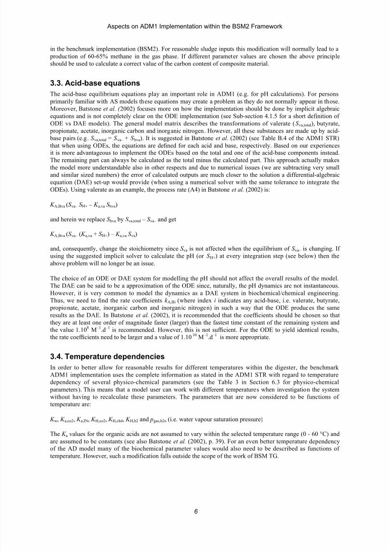
3.3. Acid-base equations

The acid-base equilibrium equations play an important role in ADM1 (e.g. for pH calculations). For persons

primarily familiar with AS models these equations may create a problem as they do not normally appear in those.

Moreover, Batstone et al. ( 2002) focuses more on how the implementation should be done by implicit algebraic

equations and is not completely clear on the ODE implementation (see Sub-section 4.1.5 for a short definition of

ODE vs DAE models). The general model matrix describes the transformations of valerate (S va,total), butyrate,

propionate, acetate, inorganic carbon and inorganic nitrogen. However, all these substances are made up by acid- base pairs (e.g. S va,total = S va– + S hva). It is suggested in Batstone et al. (2002) (see Table B.4 of the ADM1 STR)

that when using ODEs, the equations are defined for each acid and base, respectively. Based on our experiences

it is more advantageous to implement the ODEs based on the total and one of the acid-base components instead.

The remaining part can always be calculated as the total minus the calculated part. This approach actually makes

the model more understandable also in other respects and due to numerical issues (we are subtracting very small

and similar sized numbers) the error of calculated outputs are much closer to the solution a differential-algebraic

equation (DAE) set-up would provide (when using a numerical solver with the same tolerance to integrate the

ODEs). Using valerate as an example, the process rate (A4) in Batstone et al. (2002) is:

K A,Bva (S va– S H+ – K a,va S hva)

and herein we replace S hva by S va,total – S va– and get

K A,Bva (S va– ( K a,va + S H+) – K a,va S va)

and, consequently, change the stoichiometry since S va is not affected when the equilibrium of S va– is changing. If

using the suggested implicit solver to calculate the pH (or S H+) at every integration step (see below) then the

above problem will no longer be an issue.




3.5. Model equations

In the sub-sections below all the required equations for a full ODE implementation of ADM1 are given.

3.5.1. Process ratesThe biochemical process rates are defined below.

Disintegration:

cdis1 X k !="

Hydrolysis of carbohydrates:

chchhyd,2 X k !

="

Hydrolysis of proteins:

pr pr hyd,3 X k !="

Hydrolysis of lipids:

lilihyd,4 X k !="

Uptake of sugars:

5su

susuS,

susum,5 I X

S K

S k !!

+

!="

Uptake of amino-acids:

6aa

aaaaS,

aaaam,6 I X

S K

S k !!

+

!="

Uptake of LCFA (long-chain fatty acids):

fa IXS

k="




Decay of X c4:

c4Xc4dec,16 X k !="

Decay of X pro:

proXprodec,17 X k !="

Decay of X ac:

acXacdec,18 X k !="

Decay of X h2:

h2Xh2dec,19 X k !="

In the expressions for ! 8 and ! 9, a small constant (1.10 –6

) should be been added at the denominator to the sum

(S va + S bu) in order to avoid division by zero in the case of poor choice of initial conditions for S va and S bu,

respectively. Apart from this, the above equations are identical to the original ADM1.

The acid-base rates for the BSM2 ODE implementation (see Chapter 4 and Appendix 1 for the corresponding

DAE implementation) are as follows:

" A,4 = k A,Bva S va# K a,va + S

H+( )#K a,vaS va( )

" A,5 = k A,Bbu S bu # K a,bu + S H

+( )#K a,buS bu( )

" A,6 = k A,Bpro S pro# K a,pro + S

H+( )#K a,proS pro( )

" A,7 = k A,Bac S ac# K a,ac + S

H+( )#K a,acS ac( )

" A,10 = k A,Bco2 S hco3# K a,co2 + S

H+( )#K a,co2S IC( )




I pH,aa =

exp "3 pH " pH UL,aa

pH UL,aa " pH LL,aa

#

$

% &

'

(

2#

$

% %

&

'

( (

: pH < pH UL,aa

1 : pH > pH UL,aa

)

* +

, +

I pH,ac =exp "3

pH " pH UL,ac

pH UL,ac " pH LL,ac

#

$ %

&

' (

2#

$

% %

&

'

( (

: pH < pH UL,ac

1 : pH > pH UL,ac

)

* +

, +

I pH,h2 = exp "3 pH " pH UL,h2

pH UL,h2 " pH LL,h2

#

$ %

&

' (

2#

$ %

%

&

' (

( : pH < pH UL,h2

1 : pH > pH UL,h2

)

* +

, +

I IN,lim =

1

1+ K S,IN S IN

fah2,I,h2

fah2,1

1

K S I

+

=

c4h2,I,h2

c4h2,1

1

K S I

+

=

proh2,I,h2 proh2,

1

1

K S I

+

=

nh3Inh3

nh31

1

K S I

+

=




has been chosen for the ADM1 in BSM2. For the ADM1, this gives the following expressions:

aaaa

aa

pHH

pHaa pH, nn

n

K S

K

I +

=

+

with 2 pH

aaUL,aaLL,

10

pH pH

K

+

!

= andaaLL,aaUL,

aa 0.3 pH pH

n!

=

acac

ac

pHH

pHac pH, nn

n

K S

K I

+

=

+

with 2 pH

acUL,acLL,

10

pH pH

K

+

!

= and nac =3.0

pH UL,ac " pH LL,ac

h2h2

h2

pHH

pHh2 pH, nn

n

K S

K I

+

=

+

with 2 pH

h2UL,h2LL,

10

pH pH

K

+

!

= and

h2LL,h2UL,

h2

0.3

pH pH n

!

=

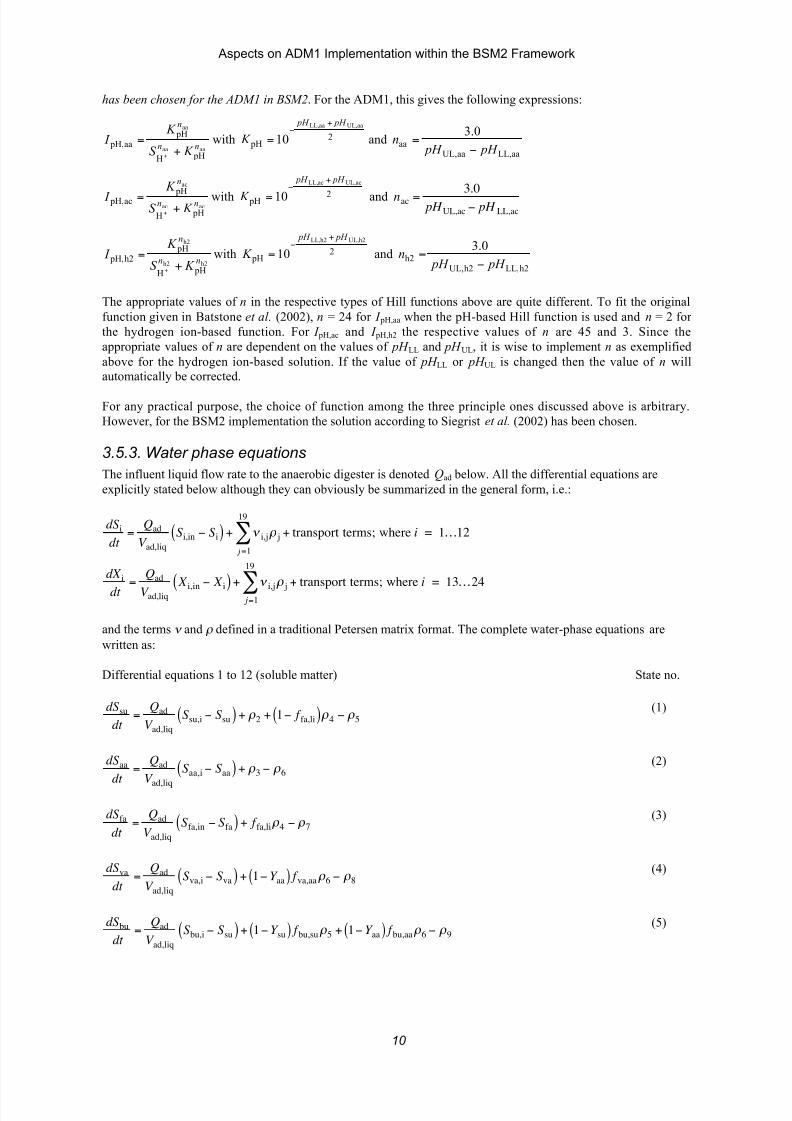
The appropriate values of n in the respective types of Hill functions above are quite different. To fit the original

function given in Batstone et al. (2002), n = 24 for I pH,aa when the pH-based Hill function is used and n = 2 for

the hydrogen ion-based function. For I pH,ac and I pH,h2 the respective values of n are 45 and 3. Since the

appropriate values of n are dependent on the values of pH LL and pH UL, it is wise to implement n as exemplified

above for the hydrogen ion-based solution. If the value of pH LL or pH UL is changed then the value of n will

automatically be corrected.

For any practical purpose, the choice of function among the three principle ones discussed above is arbitrary.However, for the BSM2 implementation the solution according to Siegrist et al. (2002) has been chosen.

3.5.3. Water phase equations

The influent liquid flow rate to the anaerobic digester is denoted Qad below. All the differential equations are

explicitly stated below although they can obviously be summarized in the general form, i.e.:

dS i

dt

=

Qad

Vad liq

S i,in " S i( ) + # i,j

19

$ % j + transport terms; where i = 1…12




dS pro

dt =

Qad

V ad,liqS pro,i " S pro( ) + 1"Y su( ) f pro,su# 5 + 1"Y aa( ) f pro,aa# 6 + 1"Y c4( ) 0.54# 8 " # 10

(6)

dS ac

dt =

Qad

V ad,liqS ac,i " S ac( ) + 1"Y su( ) f ac,su# 5 + 1"Y aa( ) f ac,aa# 6 + 1"Y fa( ) 0.7# 7

+ 1"Y c4( ) 0.31# 8 + 1"Y c4( ) 0.8# 9 + 1"Y pro( ) 0.57# 10 " # 11

(7)

dS h2

dt =

Qad

V ad,liqS h2,i " S h2( ) + 1"Y su( ) f h2,su# 5 + 1"Y aa( ) f h2,aa# 6 + 1"Y fa( ) 0.3# 7

+ 1"Y c4( ) 0.15# 8 + 1"Y c4( ) 0.2# 9 + 1"Y pro( ) 0.43# 10 " # 12 " # T,8

(8)

dS ch4

dt =

Qad

V ad,liqS ch4,i " S ch4( ) + 1"Y ac( )# 11 + 1"Y h2( )# 12 " # T,9

(9)

dS IC

dt =

Qad

V ad,liqS IC,i " S IC( ) " C k# k,j$ j

k =

1"9,11"24

%&

'

( (

)

*

+ +

j =

1

19

% " $ T ,10

(10)

see below

dS IN

dt =

Qad

V ad,liqS IN,i " S IN( ) "Y su N bac# 5 + N aa " Y aa N bac( )# 6 "Y fa N bac# 7 "Y c4 N bac# 8

"Y c4 N bac# 9 "Y pro N bac# 10 "Y ac N bac# 11 "Y h2 N bac# 12 + N bac " N xc( ) # k

k =13

19

$

+ N xc " f xi,xc N I " f si,xc N I " f pr,xc N aa( )# 1

(11)




s9 = "C bu + 1"Y c4( ) 0.8C ac +Y c4C bac

s10

= "C pro

+

1"Y

pro( ) 0.57C

ac+Y

proC

bac

s11 = "C ac + 1"Y ac( )C ch4 +Y acC bac

s12 = 1"Y h2( )C ch4 +Y h2C bac

xc bac13 C C s +!=

Differential equations 13 to 24 (particulate matter) State no.

dX c

dt =

Qad

V ad,liq X c,i " X c( ) " # 1 + # 13 + # 14 + # 15 + # 16 + # 17 + # 18 + # 19

(13)

dX ch

dt =

Qad

V ad,liq X ch,i " X ch( ) + f ch,xc# 1 " # 2

(14)

dX pr

dt

=

Qad

V ad,liq X pr,i " X pr

( )+ f pr,xc# 1 " # 3

(15)

dX li

dt =

Qad

V ad,liq X li,i " X li( ) + f li,xc# 1 " # 4

(16)

dX su

dt =

Qad

V ad,liq X su,i " X su( ) +Y su# 5 " # 13

(17)




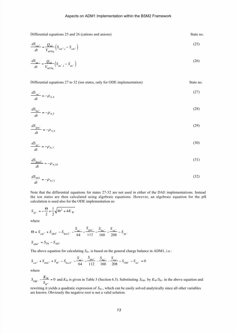
Differential equations 25 and 26 (cations and anions) State no.

dS cat

+

dt =

Qad

V ad,liqS

cat + ,i " S

cat+( ) (25)

dS an"

dt =

Qad

V ad,liqS an " ,i

" S an "( )

(26)

Differential equations 27 to 32 (ion states, only for ODE implementation) State no.

4A

va

,dt

dS ! "=

"

(27)

5A

bu

,dt

dS ! "=

"

(28)

6A

pro

,dt

dS ! "=

" (29)

7A

ac

,dt

dS ! "=

"

(30)

h 3

dS !

"

(31)




We also calculate the concentration of dissolved carbon dioxide algebraically as:

!!=

hco3ICco2 S S S

3.5.4. Gas phase equations

Differential equations 33 to 35 describe the fate of the gas phase components: State no.

gasad,

liqad,

8gaad,

gash2gas,h2gas,

V

V

V

QS

dt

dS ,T

s

!+"= #

(33)

gasad,

liqad,

9Tgasad,

gasch4gas,ch4gas,

V

V

V

QS

dt

dS , !+"= #

(34)

gasad,

liqad,

10Tgasad,

gasco2gas,co2gas,

V

V

V

QS

dt

dS , !+"= #

(35)

where Qgas denote the gas flow rate. The associated algebraic equations required for the gas transfer rates ! T,8,! T,9 and ! T,10 are:

pgas,h2 = S gas,h2 " RT ad

16

pgas,ch4 = S gas,ch4 " RT ad

64

adco2gas,co2gas, RT S p !=




are changed (volume, load etc.), for example if applying the ADM1 as a stand-alone model outside the

framework of BSM2, then the parameter k p will have to be adjusted to achieve a reasonable overpressure in the

head space.

4. ADM1 DAE IMPLEMENTATION

It has been realized that the ODE implementation is problematic for use in the BSM2 framework due to the

computational effort. Therefore, two DAE versions have been developed (Rosen et al., 2006). In this section, the

differential algebraic equation model implementations of ADM1 are presented. Two different DAE models are

discussed: a model based on algebraic pH (S H+) calculations (DAE pH) and a model based on algebraic pH and S h2

calculations (DAE pH,S h2). The second model implementation is motivated by the stiffness problem of the ODE

and DAE pH implementations.

4.1. Motivation

The fact that the Matlab/Simulink ADM1 implementation discussed here aims at being an integrated part of the

BSM2 puts some requirements on the way the ADM1 is implemented. The model must be able to handle

dynamic inputs, time-discrete and event-driven control actions as well as stochastic inputs or noise and still be

sufficiently efficient and fast to allow for extensive simulations.

4.1.1. Dynamic inputsBSM2 aims at developing and evaluating control strategies for wastewater treatment. The challenge of

controlling a WWTP lies mainly in the changing influent wastewater characteristics. The generation of dynamic

input is, thus, an integrated part of BSM2. This means that, except in order to obtain initial conditions, BSM2 is

basically always simulated using dynamic input and, consequently, no plant unit is ever at steady state.

According to the BSM2 protocol, using dynamic influent data, the plant is simulated for 63 days to reach a

pseudo steady state. This is followed by 182 days of simulation for initialisation of control and/or monitoring

algorithms. The subsequent 364 days of simulation is the actual evaluation period. In total, this encompasses 609

days of dynamic simulations with new data every 15 minutes (Gernaey et al., 2005; 2006).




solvers, predictions of future state values are carried out. However, predictions of future state values affected by

stochastic inputs will result in poor results, slowing down the solver by limiting its ability to use long integration

steps. Simulation of the BSM2 is, thus, subject to the following dilemma. BSM2, which includes ASM1 and

ADM1 models, is a very stiff system and, consequently, a stiff solver should be used. However, since BSM2 is a

control simulation benchmark, noise must be included, calling for an explicit (i.e. non-stiff) solver.

4.1.5. ODE and DAE systemsWhen the states of a system are described only by ordinary differential equations, the system is said to be an

ODE system. If the system is stiff, it is sometimes possible to rewrite some of the system equations in order to

omit the fastest states. The rationale for this is that from the slower states’ point of view, the fast states can be

considered instantaneous and possible to describe by algebraic equations. Such systems are normally referred to

as differential algebraic equation (DAE) systems. By rewriting an ODE system to a DAE system, the stiffnesscan be decreased, allowing for explicit solvers to be used and for stochastic elements to be incorporated. The

drawback is that the DAE system is only an approximation of the original system and the effect of this

approximation must be considered and investigated for each specific simulation model.

4.1.6. Time constants in ADM1As mentioned before, the ADM1 includes time constants covering a wide range; from milliseconds for pH to

weeks or months for the states describing various fractions of active biomass. Since most control actions

affecting the anaerobic digester are fairly slow, it makes sense to investigate which fast states can be

approximated by algebraic equations. In Batstone et al. (2002), it is suggested that the pH (S H+) state iscalculated by algebraic equations. However, this will only partially solve the stiffness problem. There are other

fast states and a closer investigation suggests that the state describing hydrogen ( S h2) also needs to be

approximated by an algebraic equation in order to enhance the performance when simulating the ADM1 using a

explicit solver.

4.2. DAE equations

4 2 1 H l




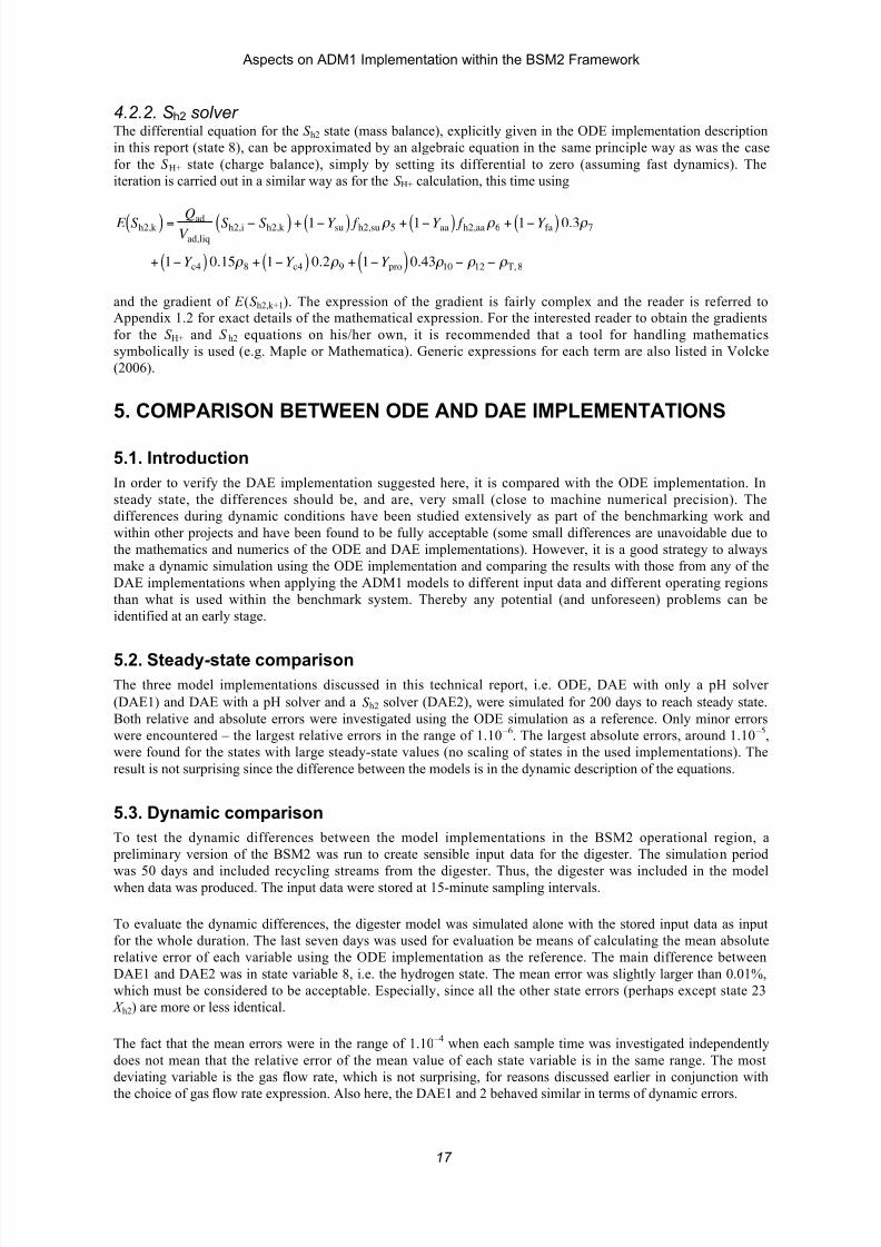
4.2.2. Sh2 solver The differential equation for the S h2 state (mass balance), explicitly given in the ODE implementation description

in this report (state 8), can be approximated by an algebraic equation in the same principle way as was the casefor the S H+ state (charge balance), simply by setting its differential to zero (assuming fast dynamics). The

iteration is carried out in a similar way as for the S H+ calculation, this time using

E S h2,k( ) =Qad

V ad,liqS h2,i " S h2,k( ) + 1" Y su( ) f h2,su# 5 + 1" Y aa( ) f h2,aa# 6 + 1" Y fa( ) 0.3# 7

+ 1" Y c4( ) 0.15# 8 + 1" Y c4( ) 0.2# 9 + 1" Y pro( ) 0.43# 10 " # 12 " # T,8

and the gradient of E (S h2,k+1). The expression of the gradient is fairly complex and the reader is referred toAppendix 1.2 for exact details of the mathematical expression. For the interested reader to obtain the gradients

for the S H+ and S h2 equations on his/her own, it is recommended that a tool for handling mathematics

symbolically is used (e.g. Maple or Mathematica). Generic expressions for each term are also listed in Volcke

(2006).

5. COMPARISON BETWEEN ODE AND DAE IMPLEMENTATIONS

5.1. IntroductionIn order to verify the DAE implementation suggested here, it is compared with the ODE implementation. In

steady state, the differences should be, and are, very small (close to machine numerical precision). The

differences during dynamic conditions have been studied extensively as part of the benchmarking work and

within other projects and have been found to be fully acceptable (some small differences are unavoidable due to

the mathematics and numerics of the ODE and DAE implementations). However, it is a good strategy to always

make a dynamic simulation using the ODE implementation and comparing the results with those from any of the

DAE implementations when applying the ADM1 models to different input data and different operating regions

h h i d i hi h b h k Th b i l ( d f ) bl b




NOTE! The choice between the three implementations of ADM1 – ODE, DAE1 and DAE2 – is up to the user. If

acceptable computation times can be achieved with the ODE or DAE1 implementations there is no other

advantage in using DAE2. However, for Matlab/Simulink it appears that with currently available solvers, DAE2

is the only practically feasible choice for BSM2.

6. ADM1 BENCHMARK MODEL PARAMETERS

In the sections below the ADM1 parameters used for the BSM2 implementation are presented. In cases where

the parameter value in ADM1 for BSM2 differs from the default ADM1 parameter value (Batstone et al., 2002)

the explicit row is marked in grey and the default value is given in the commentary field. In a few cases it is not

really possible to determine explicitly what the ADM1 suggested default parameter values are, since several possible values may be stated (depending on temperature, different references, etc.) or no value at all is given (in

some cases the selected values below are based on the original ADM1 implementation in AquaSim by the

ADM1 Task Group). Also, in cases where different options have been given for mesophilic high rate, mesophilic

solids and thermophilic solids AD systems in Batstone et al. (2002), the values below refer to mesophilic solids

systems.

Obviously many of the parameter values are application specific and should, if possible, be determined or

estimated based on measured data. However, for the purpose of the BSM2, the values suggested below produce

satisfactory results. It should be noted that the parameter values for the hydrolysis rates (10 d

–1

) used in bothADM1-BSM2 and given as default parameter values in the ADM1 STR are nowadays considered to be at least

ten times too large (Batstone 2002-2008, personal communication).

6.1. Stoichiometric parameter values

Table 1: Stoichiometric parameter values for the BSM2 ADM1 implementation

Parameter Value Unit Process(es) Comments

f 0 1 1




Not stated in ADM1 STR but value of 0.03

used in original TG AquaSim implementatio

f fa,li 0.95 – 4

C fa 0.0217 kmole C.kg –1 COD 4, 7 C 3 in state equation 10

f h2,su 0.19 – 5

f bu,su 0.13 – 5

f pro,su 0.27 – 5

f ac,su 0.41 – 5

N bac 0.08/14 kmole N.kg –1

COD 5-19 ADM1 default value = 0.00625

Here: 8% on weight basis based on ASM1

C bu 0.025 kmole C.kg –1

COD 5, 6, 9 C 5 in state equation 10

C pro 0.0268 kmole C.kg –1

COD 5, 6, 8, 10 C 6 in state equation 10

C ac 0.0313 kmole C.kg –1 COD 5-11 C 7 in state equation 10

C bac 0.0313 kmole C.kg –1

COD 5-19 C 17–23 in state equation 10

Y su 0.1 – 5 kmole CODX.kg –1

CODS

f h2,aa 0.06 – 6

f va,aa 0.23 – 6

f bu,aa 0.26 – 6

f pro,aa 0.05 – 6

f ac,aa 0.40 – 6

C va 0.024 kmole C.kg –1

COD 6, 8 C 4 in state equation 10

Y aa 0.08 – 6 kmole CODX.kg –1 CODS

Y fa 0.06 – 7 kmole CODX.kg –1

CODS

Y c4 0.06 – 8, 9 kmole CODX.kg –1

CODS

Y pro 0.04 – 10 kmole CODX.kg –1

CODS

C ch4 0.0156 kmole C.kg –1

COD 11, 12 C 9 in state equation 10

Y ac 0.05 – 11 kmole CODX.kg –1

CODS

Y h2 0.06 – 12 kmole CODX.kg –1

CODS

Note that C h2 and C IN, i.e. C 8 and C 11, are equal to zero in state equation 10 (S IC)




pH LL,ac 6 - 11 in process inhibition equation I 11

k m,h2 35 d-1

12

K S,h2 7.10-6

kg COD.m-3

12

pH UL,h2 6 - 12 in process inhibition equation I 12

pH LL,h2 5 - 12 in process inhibition equation I 12

k dec,Xsu 0.02 d-1

13

k dec,Xaa 0.02 d-1

14

k dec,Xfa 0.02 d-1

15

k dec,Xc4 0.02 d-1

16

k dec,Xpro 0.02 d-1

17

k dec,Xac 0.02 d-1

18

k dec,Xh2 0.02 d-1

13

The unit M is defined as kmole m –3

according to Batstone et al. (2002)

6.3. Physico-chemical parameter values

Table 3: Physico-chemical parameter values for the BSM2 ADM1 implementation

Parameter Value Unit Comments

R 0.083145 bar.M-1

.K -1

ADM1 default value = 0.08314

T base 298.15 K ADM1 default value = 298T ad 308.15 K = 35°C

K w10

-14.0

exp 55900

100 " R" 1

T base

# 1

T ad

$

% &

'

( )

$

% & &

'

( ) )

M ! 2.08·10-14

K a,va 10-4.86

M ! 1.38·10-5

K a,bu 10-4.82

M ! 1.5·10-5

K a,pro 10-4.88

M ! 1.32·10-5

K a,ac 10-4.76

M ! 1.74·10-5

K $ '$ ' M ! 4 94 10 7




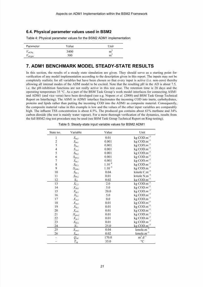
6.4. Physical parameter values used in BSM2

Table 4: Physical parameter values for the BSM2 ADM1 implementation

Parameter Value Unit

V ad,liq 3400 m3

V ad,gas 300 m3

7. ADM1 BENCHMARK MODEL STEADY-STATE RESULTS

In this section, the results of a steady state simulation are given. They should serve as a starting point for

verification of any model implementation according to the description given in this report. The inputs may not be

completely realistic for all variables but have been chosen so that every input is active (i.e. non-zero) thereby

allowing all internal modes of the ADM model to be excited. Note that the resulting pH in the AD is about 7.5,

i.e. the pH-inhibition functions are not really active in this test case. The retention time is 20 days and the

operating temperature 35 °C. As a part of the BSM Task Group’s work model interfaces for connecting ASM1

and ADM1 (and vice versa) have been developed (see e.g. Nopens et al. (2008) and BSM Task Group Technical

Report on Interfacing). The ASM1 to ADM1 interface fractionates the incoming COD into inerts, carbohydrates,

proteins and lipids rather than putting the incoming COD into the ADM1 as composite material. Consequently,

the composite material value in this example is low and the values of the other input variables are comparably

high. The influent TSS concentration is about 4.5%. The produced gas contains about 61% methane and 34%

carbon dioxide (the rest is mainly water vapour). For a more thorough verification of the dynamics, results from

the full BSM2 ring test procedure may be used (see BSM Task Group Technical Report on Ring-testing).

Table 5: Steady-state input variable values for BSM2 ADM1

State no. Variable Value Unit

1 S su,i 0.01 kg COD.m –3

3




Table 6: Steady-state output variable values for BSM2 ADM1

State no. Variable Value Unit

1 S su 0.011954829716958 kg COD.m –3

2 S aa 0.005314740171633 kg COD.m –3

3 S fa 0.098621400930799 kg COD.m –3

4 S va 0.011625006463861 kg COD.m –3

5 S bu 0.013250729666269 kg COD.m –3

6 S pro 0.015783666284542 kg COD.m –3

7 S ac 0.197629716937552 kg COD.m –3

8 S h2 0.000000235945059 kg COD.m –3

9 S ch4 0.055088776445959 kg COD.m –3

10 S IC 0.152677870626333 kmole C.m –3

11 S IN 0.130229815803682 kmole N.m –3

12 S I 0.328697663721532 kg COD.m –3

13 X C 0.308697663721532 kg COD.m –3

14 X ch 0.027947240435040 kg COD.m –3

15 X pr 0.102574106106682 kg COD.m –3

16 X li 0.029483049707287 kg COD.m –3

17 X su 0.420165982454567 kg COD.m –3

18 X aa 1.179171798923700 kg COD.m –3

19 X fa 0.243035344719442 kg COD.m –3

20 X c4 0.431921105635979 kg COD.m –3

21 X pro 0.137305908933954 kg COD.m –3

22 X ac 0.760562658313215 kg COD.m –3

23 X h2 0.317022953361272 kg COD.m –3

24 X I 25.617395327443063 kg COD.m –3

25 S cat 0.040000000000000 kmole.m –3

26 S an 0.020000000000000 kmole.m –3

Q 1 0 0000000000000 3 d 1




8. SIMULATION EFFICIENCY ANALYSIS

To evaluate the model implementations described in this report, a number of simulation tests were carried out.

These tests included 1) steady-state simulations, 2) dynamic simulations for two weeks to compare the transient

behaviour in detail and 3) dynamic simulations for 609 days to compare overall simulation times. The model

implementations investigated were:

1. ODE – the differential equation implementation;

2. DAE1 – differential equations with algebraic solution of pH (S H+);

3. DAE2 – differential equations with algebraic solution of pH and S h2.

All three models were tested as a part of the BSM2. This means that the behaviour reported here refers to the

whole BSM2 system. The simulations were carried out using a standard PC running Windows XP andMatlab/Simulink Release 13. The ASM1, the clarifiers and the ADM1 were all implemented as MEX-files based

on C source code.

8.1. Steady state simulations

The three model implementations were simulated for 200 days to reach steady state. Both relative and absolute

errors were investigated using the ODE simulation as a reference. Only minor errors were encountered – the

largest relative errors in the range of 10-6

. The largest absolute errors, 10-5

, were found in the states with large

steady-state values (no scaling of states in the implementations). The result is not surprising since the difference between the models is in the dynamic description of the equations.

8.2. Transient behaviour

Although the model implementations differ in the description of pH and S h2 dynamics, no significant differences

were obtained when the transients in the states were investigated. The relative errors are typically in the range of

10-6

or smaller, again using the ODE implementation as reference. However, one important exception is the gas

flow rate. Although not a true state of the model, the gas flow rate seems to be highly sensitive to the integration

l i h d h l h d h f l l d i b h i i h fl




Rewriting the ODE system into a DAE system, representing both the pH and S h2 state by algebraic equations,

yields a significant simulation time reduction. As seen in Table 7, the improvement when noise and discrete

sensors are present is significant. This also holds in the absence of noise or when discrete sensors are

implemented. Compared to the ODE system or the DAE1 system, an increase in speed by a factor 8 is achieved

(ODE* simulation time: 4, DAE1* simulation time: 4 and DAE2* simulation time: 0.5, see Table 7).

101

102

103

104

105

106

107

-real(? )

imag(

?)

ODE

DAE1

DAE2SH+S

h2

Figure 1. The eigenvalues of the linearised systems. Note the logarithmic scale and that small the

values are not shown (x-axis: –real(#), y-axis: im(#)).

9. REFERENCES

Batstone D.J., Keller J., Angelidaki I., Kalyuzhnyi S.V., Pavlostathis S.G., Rozzi A., Sanders W.T.M., Siegrist

H. and Vavilin V.A. (2002). Anaerobic Digestion Model No. 1. IWA STR No. 13, IWA Publishing,

London, UK.

Copp J.B. (ed.) (2002). The COST Simulation Benchmark – Description and Simulator Manual . ISBN 92-894-

1658-0, Office for Official Publications of the European Communities, Luxembourg.

Gernaey K.V., Rosen C., Benedetti L. and Jeppsson U. (2005). Phenomenological modelling of wastewater treat-

ment plant influent disturbances scenarios. 10th

International Conference on Urban Drainage (10ICUD),

21-26 August, Copenhagen, Denmark.




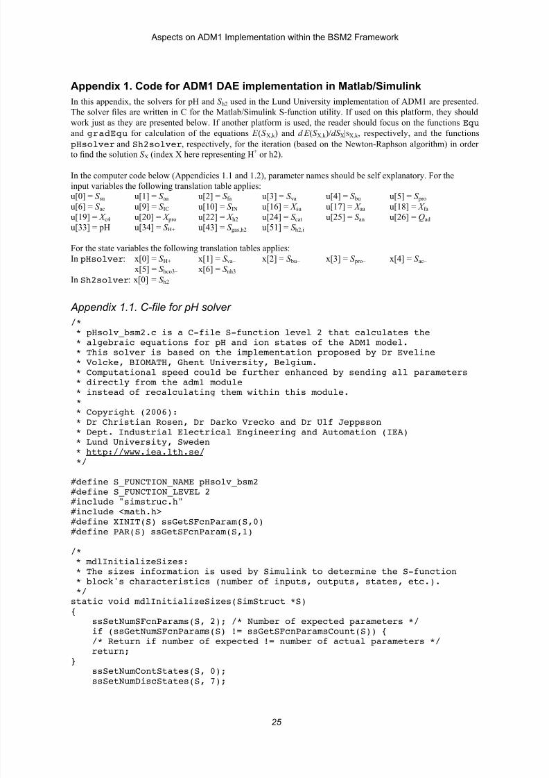
Appendix 1. Code for ADM1 DAE implementation in Matlab/Simulink

In this appendix, the solvers for pH and S h2 used in the Lund University implementation of ADM1 are presented.

The solver files are written in C for the Matlab/Simulink S-function utility. If used on this platform, they should

work just as they are presented below. If another platform is used, the reader should focus on the functions Equand gradEqu for calculation of the equations E (S X,k ) and d E (S X,k )/dS X|SX,k , respectively, and the functions

pHsolver and Sh2solver, respectively, for the iteration (based on the Newton-Raphson algorithm) in order

to find the solution S X (index X here representing H+ or h2).

In the computer code below (Appendicies 1.1 and 1.2), parameter names should be self explanatory. For the

input variables the following translation table applies:

u[0] = S su u[1] = S aa u[2] = S fa u[3] = S va u[4] = S bu u[5] = S pro

u[6] = S ac u[9] = S IC u[10] = S IN u[16] = X su u[17] = X aa u[18] = X fau[19] = X c4 u[20] = X pro u[22] = X h2 u[24] = S cat u[25] = S an u[26] = Qad

u[33] = pH u[34] = S H+ u[43] = S gas,h2 u[51] = S h2,i

For the state variables the following translation tables applies:

In pHsolver: x[0] = S H+ x[1] = S va– x[2] = S bu– x[3] = S pro– x[4] = S ac–

x[5] = S hco3– x[6] = S nh3

In Sh2solver: x[0] = S h2

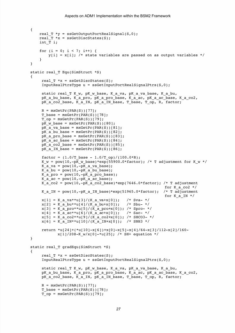
Appendix 1.1. C-file for pH solver

/* * pHsolv_bsm2.c is a C-file S-function level 2 that calculates the * algebraic equations for pH and ion states of the ADM1 model. * This solver is based on the implementation proposed by Dr Eveline * Volcke, BIOMATH, Ghent University, Belgium. * Computational speed could be further enhanced by sending all parameters




if (!ssSetNumInputPorts(S, 1)) return; ssSetInputPortWidth(S, 0, 51); /*(S, port index, port width)*/ ssSetInputPortDirectFeedThrough(S, 0, 0);

if (!ssSetNumOutputPorts(S, 1)) return; ssSetOutputPortWidth(S, 0, 7); ssSetNumSampleTimes(S, 1); ssSetOptions(S, SS_OPTION_EXCEPTION_FREE_CODE);}

/* * mdlInitializeSampleTimes: * This function is used to specify the sample time(s) for your

* S-function. You must register the same number of sample times as * specified in ssSetNumSampleTimes. */static void mdlInitializeSampleTimes(SimStruct *S){ ssSetSampleTime(S, 0, INHERITED_SAMPLE_TIME); /* executes whenever driving block executes */ ssSetOffsetTime(S, 0, 0.0);}

#define MDL_INITIALIZE_CONDITIONS /* Change to #undef to remove function */#if defined(MDL_INITIALIZE_CONDITIONS)/* mdlInitializeConditions: * In this function, you should initialize the continuous and discrete * states for your S-function block. The initial states are placed * in the state vector, ssGetContStates(S) or ssGetRealDiscStates(S). * You can also perform any other initialization activities that your * S-function may require. Note, this routine will be called at the * start of simulation and if it is present in an enabled subsystem




{ real_T *y = ssGetOutputPortRealSignal(S,0); real_T *x = ssGetDiscStates(S);

int_T i;

for (i = 0; i < 7; i++) { y[i] = x[i]; /* state variables are passed on as output variables */ }}

static real_T Equ(SimStruct *S){

real_T *x = ssGetDiscStates(S); InputRealPtrsType u = ssGetInputPortRealSignalPtrs(S,0);

static real_T K_w, pK_w_base, K_a_va, pK_a_va_base, K_a_bu, pK_a_bu_base, K_a_pro, pK_a_pro_base, K_a_ac, pK_a_ac_base, K_a_co2, pK_a_co2_base, K_a_IN, pK_a_IN_base, T_base, T_op, R, factor;

R = mxGetPr(PAR(S))[77]; T_base = mxGetPr(PAR(S))[78]; T_op = mxGetPr(PAR(S))[79];

pK_w_base = mxGetPr(PAR(S))[80]; pK_a_va_base = mxGetPr(PAR(S))[81]; pK_a_bu_base = mxGetPr(PAR(S))[82]; pK_a_pro_base = mxGetPr(PAR(S))[83]; pK_a_ac_base = mxGetPr(PAR(S))[84]; pK_a_co2_base = mxGetPr(PAR(S))[85]; pK_a_IN_base = mxGetPr(PAR(S))[86];

factor = (1.0/T_base - 1.0/T_op)/(100.0*R);




pK_w_base = mxGetPr(PAR(S))[80]; pK_a_va_base = mxGetPr(PAR(S))[81]; pK_a_bu_base = mxGetPr(PAR(S))[82];

pK_a_pro_base = mxGetPr(PAR(S))[83]; pK_a_ac_base = mxGetPr(PAR(S))[84]; pK_a_co2_base = mxGetPr(PAR(S))[85]; pK_a_IN_base = mxGetPr(PAR(S))[86];

factor = (1.0/T_base - 1.0/T_op)/(100.0*R); K_w = pow(10,-pK_w_base)*exp(55900.0*factor); /* T adjustment for K_w */ K_a_va = pow(10,-pK_a_va_base); K_a_bu = pow(10,-pK_a_bu_base);

K_a_pro = pow(10,-pK_a_pro_base); K_a_ac = pow(10,-pK_a_ac_base); K_a_co2 = pow(10,-pK_a_co2_base)*exp(7646.0*factor); /* T adjustment

for K_a_co2 */ K_a_IN = pow(10,-pK_a_IN_base)*exp(51965.0*factor); /* T adjustment

for K_a_IN */

return 1+K_a_IN**u[10]/((K_a_IN+x[0])*(K_a_IN+x[0])) +K_a_co2**u[9]/((K_a_co2+x[0])*(K_a_co2+x[0])) +1/64.0*K_a_ac**u[6]/((K_a_ac+x[0])*(K_a_ac+x[0]))

+1/112.0*K_a_pro**u[5]/((K_a_pro+x[0])*(K_a_pro+x[0])) +1/160.0*K_a_bu**u[4]/((K_a_bu+x[0])*(K_a_bu+x[0])) +1/208.0*K_a_va**u[3]/((K_a_va+x[0])*(K_a_va+x[0])) +K_w/(x[0]*x[0]); /* Gradient of SH+ equation */}

static void pHsolver(SimStruct *S){




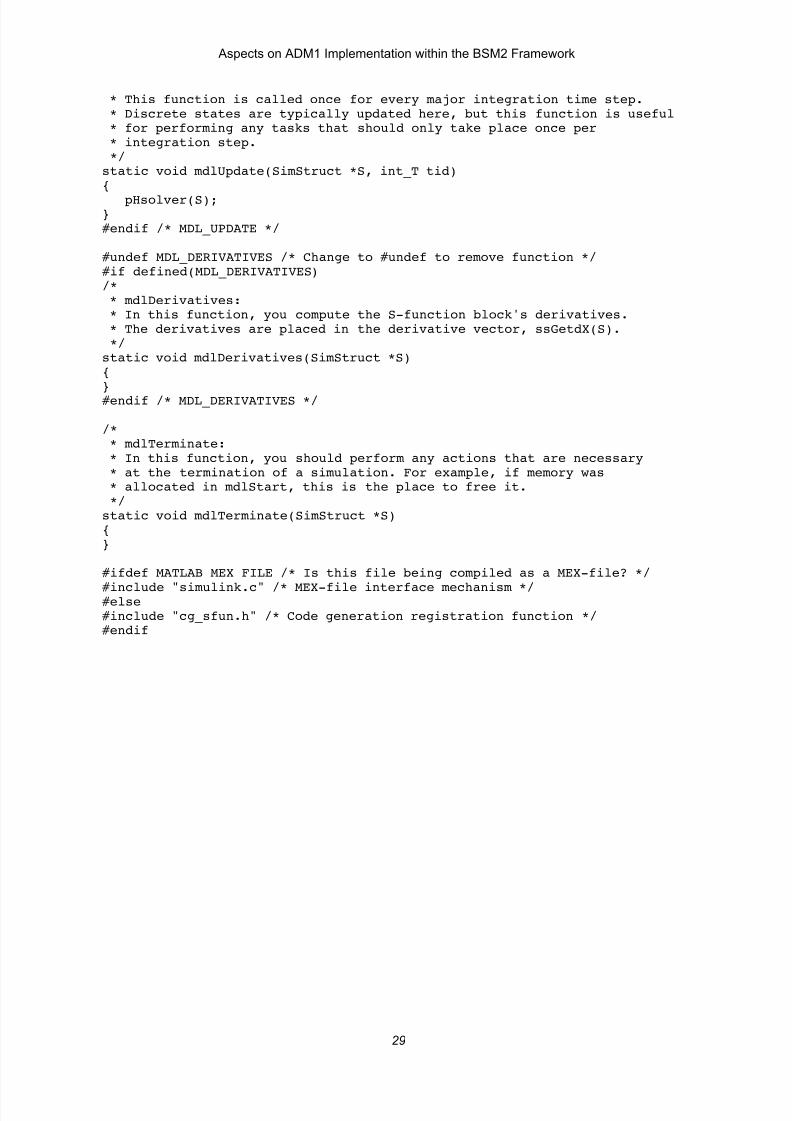
* This function is called once for every major integration time step. * Discrete states are typically updated here, but this function is useful * for performing any tasks that should only take place once per

* integration step. */static void mdlUpdate(SimStruct *S, int_T tid){ pHsolver(S);}#endif /* MDL_UPDATE */

#undef MDL_DERIVATIVES /* Change to #undef to remove function */

#if defined(MDL_DERIVATIVES)/* * mdlDerivatives: * In this function, you compute the S-function block's derivatives. * The derivatives are placed in the derivative vector, ssGetdX(S). */static void mdlDerivatives(SimStruct *S){}#endif /* MDL_DERIVATIVES */

/* * mdlTerminate: * In this function, you should perform any actions that are necessary * at the termination of a simulation. For example, if memory was * allocated in mdlStart, this is the place to free it. */static void mdlTerminate(SimStruct *S){




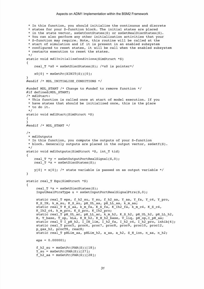
Appendix 1.2. C-file for Sh2 solver

/* * Sh2solv_bsm2.c is a C-file S-function level 2 that solves the algebraic * equation for Sh2 of the ADM1 model, * thereby reducing the stiffness of the system considerably (if used * together with a pHsolver). * * Copyright (2006): * Dr Christian Rosen, Dr Darko Vrecko and Dr Ulf Jeppsson * Dept. Industrial Electrical Engineering and Automation (IEA)

* Lund University, Sweden * http://www.iea.lth.se/ */

#define S_FUNCTION_NAME Sh2solv_bsm2#define S_FUNCTION_LEVEL 2#include "simstruc.h"#include <math.h>#define XINIT(S) ssGetSFcnParam(S,0)#define PAR(S) ssGetSFcnParam(S,1)#define V(S) ssGetSFcnParam(S,2)

/* * mdlInitializeSizes: * The sizes information is used by Simulink to determine the S-function * block's characteristics (number of inputs, outputs, states, etc.). */static void mdlInitializeSizes(SimStruct *S){




* In this function, you should initialize the continuous and discrete * states for your S-function block. The initial states are placed * in the state vector, ssGetContStates(S) or ssGetRealDiscStates(S).

* You can also perform any other initialization activities that your * S-function may require. Note, this routine will be called at the * start of simulation and if it is present in an enabled subsystem * configured to reset states, it will be call when the enabled subsystem * restarts execution to reset the states. */static void mdlInitializeConditions(SimStruct *S){ real_T *x0 = ssGetDiscStates(S); /*x0 is pointer*/

x0[0] = mxGetPr(XINIT(S))[0];}#endif /* MDL_INITIALIZE_CONDITIONS */

#undef MDL_START /* Change to #undef to remove function */#if defined(MDL_START)/* mdlStart: * This function is called once at start of model execution. If you * have states that should be initialized once, this is the place

* to do it. */static void mdlStart(SimStruct *S){}#endif /* MDL_START */

/* * mdlOutputs




Y_aa = mxGetPr(PAR(S))[34]; Y_fa = mxGetPr(PAR(S))[35]; Y_c4 = mxGetPr(PAR(S))[36];

Y_pro = mxGetPr(PAR(S))[37]; K_S_IN = mxGetPr(PAR(S))[45]; k_m_su = mxGetPr(PAR(S))[46]; K_S_su = mxGetPr(PAR(S))[47]; pH_UL_aa = mxGetPr(PAR(S))[48]; pH_LL_aa = mxGetPr(PAR(S))[49]; k_m_aa = mxGetPr(PAR(S))[50]; K_S_aa = mxGetPr(PAR(S))[51]; k_m_fa = mxGetPr(PAR(S))[52];

K_S_fa = mxGetPr(PAR(S))[53]; K_Ih2_fa = mxGetPr(PAR(S))[54]; k_m_c4 = mxGetPr(PAR(S))[55]; K_S_c4 = mxGetPr(PAR(S))[56]; K_Ih2_c4 = mxGetPr(PAR(S))[57]; k_m_pro = mxGetPr(PAR(S))[58]; K_S_pro = mxGetPr(PAR(S))[59]; K_Ih2_pro = mxGetPr(PAR(S))[60]; pH_UL_ac = mxGetPr(PAR(S))[64]; pH_LL_ac = mxGetPr(PAR(S))[65];

k_m_h2 = mxGetPr(PAR(S))[66]; K_S_h2 = mxGetPr(PAR(S))[67]; pH_UL_h2 = mxGetPr(PAR(S))[68]; pH_LL_h2 = mxGetPr(PAR(S))[69]; R = mxGetPr(PAR(S))[77]; T_base = mxGetPr(PAR(S))[78]; T_op = mxGetPr(PAR(S))[79]; kLa = mxGetPr(PAR(S))[94]; K_H_h2_base = mxGetPr(PAR(S))[98];




proc9 = k_m_c4**u[4]/(K_S_c4+*u[4])**u[19]**u[4]/(*u[3]+*u[4]+eps)*inhib[2]; proc10 = k_m_pro**u[5]/(K_S_pro+*u[5])**u[20]*inhib[3];

proc12 = k_m_h2*x[0]/(K_S_h2+x[0])**u[22]*inhib[5];

p_gas_h2 = *u[43]*R*T_op/16.0; procT8 = kLa*(x[0]-16.0*K_H_h2*p_gas_h2);

reac8 = (1.0-Y_su)*f_h2_su*proc5+(1.0-Y_aa)*f_h2_aa*proc6+(1.0- Y_fa)*0.3*proc7+(1.0-Y_c4)*0.15*proc8+(1.0-Y_c4)*0.2*proc9+(1.0- Y_pro)*0.43*proc10-proc12-procT8;

return 1/V_liq**u[26]*(*u[51]-x[0])+reac8; /* Sh2 equation */}

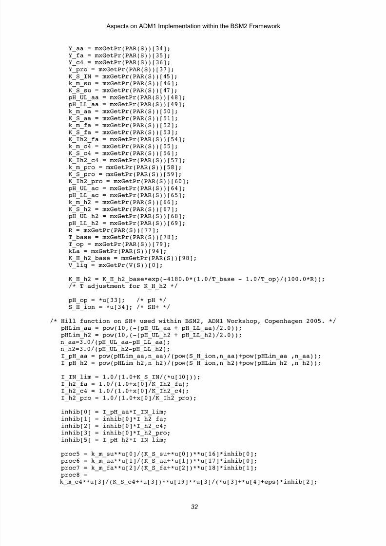
static real_T gradEqu(SimStruct *S){ real_T *x = ssGetDiscStates(S); InputRealPtrsType u = ssGetInputPortRealSignalPtrs(S,0);

static real_T eps, f_h2_su, Y_su, f_h2_aa, Y_aa, Y_fa, Y_c4, Y_pro, K_S_IN, k_m_su, K_S_su, pH_UL_aa, pH_LL_aa, k_m_aa;

static real_T K_S_aa, k_m_fa, K_S_fa, K_Ih2_fa, k_m_c4, K_S_c4, K_Ih2_c4, k_m_pro, K_S_pro, K_Ih2_pro; static real_T pH_UL_ac, pH_LL_ac, k_m_h2, K_S_h2, pH_UL_h2, pH_LL_h2, R, T_base, T_op, kLa, K_H_h2, K_H_h2_base, V_liq, pH_op, I_pH_aa, I_pH_h2; static real_T pHLim_aa, pHLim_h2, a_aa, a_h2, S_H_ion, n_aa, n_h2;

eps = 0.000001;




kLa = mxGetPr(PAR(S))[94]; K_H_h2_base = mxGetPr(PAR(S))[98]; V_liq = mxGetPr(V(S))[0];

K_H_h2 = K_H_h2_base*exp(-4180.0*(1.0/T_base - 1.0/T_op)/(100.0*R)); /* T adjustment for K_H_h2 */

pH_op = *u[33]; /* pH */ S_H_ion = *u[34]; /* SH+ */

/* Hill function on SH+ used within BSM2, ADM1 Workshop, Copenhagen 2005. */ pHLim_aa = pow(10,(-(pH_UL_aa + pH_LL_aa)/2.0));

pHLim_h2 = pow(10,(-(pH_UL_h2 + pH_LL_h2)/2.0)); n_aa=3.0/(pH_UL_aa-pH_LL_aa); n_h2=3.0/(pH_UL_h2-pH_LL_h2); I_pH_aa = pow(pHLim_aa,n_aa)/(pow(S_H_ion,n_aa)+pow(pHLim_aa ,n_aa)); I_pH_h2 = pow(pHLim_h2,n_h2)/(pow(S_H_ion,n_h2)+pow(pHLim_h2 ,n_h2));

/* Gradient of Sh2 equation */ return -1/V_liq**u[26]-3.0/10.0*(1-Y_fa)*k_m_fa**u[2]/(K_S_fa+*u[2]) **u[18]*I_pH_aa/(1+K_S_IN/(*u[10]))/((1+x[0]/K_Ih2_fa) *(1+x[0]/K_Ih2_fa))/K_Ih2_fa-3.0/20.0*(1-Y_c4)*k_m_c4**u[3]**u[3]

/(K_S_c4+*u[3])**u[19]/(*u[4]+*u[3]+eps)*I_pH_aa/(1+K_S_IN/(*u[10])) /((1+x[0]/K_Ih2_c4)*(1+x[0]/K_Ih2_c4))/K_Ih2_c4-1.0/5.0*(1- Y_c4)*k_m_c4**u[4]**u[4]/(K_S_c4+*u[4])**u[19]/(*u[4]+*u[3]+eps) *I_pH_aa/(1+K_S_IN/(*u[10]))/((1+x[0]/K_Ih2_c4)*(1+x[0]/K_Ih2_c4)) /K_Ih2_c4-43.0/100.0*(1-Y_pro)*k_m_pro**u[5]/(K_S_pro+*u[5])**u[20] *I_pH_aa/(1+K_S_IN/(*u[10]))/((1+x[0]/K_Ih2_pro)*(1+x[0]/K_Ih2_pro)) /K_Ih2_pro-k_m_h2/(K_S_h2+x[0])**u[22]*I_pH_h2/(1+K_S_IN/(*u[10])) +k_m_h2*x[0]/((K_S_h2+x[0])*(K_S_h2+x[0]))**u[22]*I_pH_h2 /(1+K_S_IN/(*u[10]))-kLa;




#define MDL_UPDATE /* Change to #undef to remove function */#if defined(MDL_UPDATE)/*

* mdlUpdate: * This function is called once for every major integration time step. * Discrete states are typically updated here, but this function is useful * for performing any tasks that should only take place once per * integration step. */static void mdlUpdate(SimStruct *S, int_T tid){ Sh2solver(S);

}#endif /* MDL_UPDATE */

#undef MDL_DERIVATIVES /* Change to #undef to remove function */#if defined(MDL_DERIVATIVES)/* * mdlDerivatives: * In this function, you compute the S-function block's derivatives. * The derivatives are placed in the derivative vector, ssGetdX(S). */

static void mdlDerivatives(SimStruct *S){}#endif /* MDL_DERIVATIVES */

/* * mdlTerminate: * In this function, you should perform any actions that are necessary * at the termination of a simulation. For example, if memory was




36

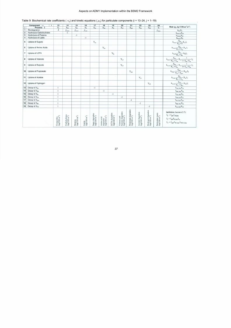
Appendix 2. Petersen matrix representation of original ADM1

The complete Petersen matrix describing the liquid phase reactions in the original ADM1 is shown below (from Batstone et al., 2002).

Table 8: Biochemical rate coefficients (! i,j) and kinetic equations (" i,j) for soluble components (i = 1–12, j = 1–19)




37

Table 9: Biochemical rate coefficients (! i,j) and kinetic equations (" i,j) for particulate components (i = 13–24, j = 1–19)

aspects on adm1 implementation within the bsm2 framework

Documents