aspen energy analyzer interface guidenuno/iip/aspen energy... · retrofit mode, and heat...
TRANSCRIPT
Interface Guide
Aspen Energy Analyzer

Version Number: V8.8May 2015
Copyright © 1981 - 2015 Aspen Technology, Inc. All rights reserved.
Aspen Energy Analyzer, HX-net, and the aspen leaf logo are trademarks or registered trademarks of AspenTechnology, Inc., Bedford, MA.
All other brand and product names are trademarks or registered trademarks of their respective companies.
This document is intended as a guide to using AspenTech's software. This documentation contains AspenTechproprietary and confidential information and may not be disclosed, used, or copied without the prior consent ofAspenTech or as set forth in the applicable license.
Although AspenTech has tested the software and reviewed the documentation, the sole warranty for the softwaremay be found in the applicable license agreement between AspenTech and the user. ASPENTECH MAKES NOWARRANTY OR REPRESENTATION, EITHER EXPRESSED OR IMPLIED, WITH RESPECT TO THIS DOCUMENTATION,ITS QUALITY, PERFORMANCE, MERCHANTABILITY, OR FITNESS FOR A PARTICULAR PURPOSE.
Aspen Technology, Inc.20 Crosby DriveBedford, MA 01730USA
Phone: (781) 221-6400Toll free: (888) 996-7001Website http://www.aspentech.com

Contents iii
Table of Contents
Technical Support ...................................................................................................1
Online Technical Support Center ........................................................................1Phone and E-mail .............................................................................................2
1 Interface ..............................................................................................................3
Structure Terminology ......................................................................................3Desktop Terminology........................................................................................4
Menu Bar ..............................................................................................4Toolbar .................................................................................................6
View Terminology.............................................................................................6Active Location ......................................................................................7Views Functionality.................................................................................7Minimized Views.....................................................................................8Modal vs. Non-Modal Views .....................................................................8Project View ..........................................................................................9
Interface Terminology..................................................................................... 12Cells & Fields ....................................................................................... 14
Maneuvering Through the Interface ................................................................. 14Hot Keys - ALT Key .............................................................................. 14Moving Through a View......................................................................... 16Entering Data ...................................................................................... 17Closing Views ...................................................................................... 19
Trace Window................................................................................................ 20Opening and Sizing the Window ............................................................. 20Available Information............................................................................ 20Object Inspect Menu............................................................................. 20
2 File Menu Options...............................................................................................23
File Menu ...................................................................................................... 23New Command .............................................................................................. 24Open Command ............................................................................................. 25Save Command ............................................................................................. 26Save As Command ......................................................................................... 27File Description .............................................................................................. 28Print Commands ............................................................................................ 28
Printing Datasheet................................................................................ 29Printing Plots ....................................................................................... 31
Exit Command ............................................................................................... 32
3 Edit, Managers, & Features Menu Options ..........................................................33
Edit Menu...................................................................................................... 33Managers Menu.............................................................................................. 33

iv Contents
Aspen Energy Analyzer ......................................................................... 33Features Menu ............................................................................................... 34
Aspen Energy Analyzer ......................................................................... 34
4 Tools Menu Options............................................................................................35
Tools Menu.................................................................................................... 35Script Manager Command ............................................................................... 36
Recording............................................................................................ 36Playback ............................................................................................. 37
Macro Language Editor.................................................................................... 38Preferences ................................................................................................... 38
General Tab......................................................................................... 39Variables Tab....................................................................................... 41Reports Tab......................................................................................... 48Files Tab ............................................................................................. 52Resources Tab ..................................................................................... 54
5 Window & Help Menu Options ............................................................................61
Window Menu ................................................................................................ 61Save Workspace .................................................................................. 62Load Workspace................................................................................... 62
Help Menu..................................................................................................... 63Adding a Bug Report............................................................................. 64Editing a Bug Report............................................................................. 65Deleting a Bug Report........................................................................... 65
6 Object Inspect Menu ..........................................................................................67
Object Inspect Menu....................................................................................... 67Empty Area in a View ..................................................................................... 67Text Editor .................................................................................................... 68Plot Area ....................................................................................................... 68
Two Axes Plots..................................................................................... 68Triangle Plots....................................................................................... 69Quaternary Plots .................................................................................. 69
Project View .................................................................................................. 73Viewer Pane ........................................................................................ 73Worksheet Pane ................................................................................... 76Main Pane ........................................................................................... 76
PFD .............................................................................................................. 77Grid Diagram................................................................................................. 77
Grid Diagram Objects ........................................................................... 79Operation Mode ............................................................................................. 79
What If Analysis View ........................................................................... 80Trend Analysis View.............................................................................. 80
7 Plot Properties ...................................................................................................83
Introduction .................................................................................................. 83Graph Control View ........................................................................................ 84
Data Tab............................................................................................. 85Axes Tab............................................................................................. 86Title Tab ............................................................................................. 88

Contents v
Legend Tab ......................................................................................... 90Plot Area Tab....................................................................................... 92
Values .......................................................................................................... 94Copy to Clipboard........................................................................................... 95Print Plot....................................................................................................... 96
Print Setup .......................................................................................... 96Plot Orientation View ...................................................................................... 97
8 Sizing and Costing..............................................................................................99
Utility Database View...................................................................................... 99Adding a New Utility ........................................................................... 101Deleting a Utility ................................................................................ 101Saving the Utility Database ................................................................. 101Recalling a Utility Database ................................................................. 102
9 References .......................................................................................................105


Technical Support 1
Technical Support
Online Technical SupportCenterAspenTech customers with a valid license and software maintenanceagreement can register to access the Online Technical Support Center at:
https://support.aspentech.com.
You use the Online Technical Support Center to:
• Access current product documentation.
• Search for technical tips, solutions, and frequently asked questions(FAQs).
• Search for and download application examples.
• Search for and download service packs and product updates.
• Submit and track technical issues.
• Search for and review known limitations.
• Send suggestions.
Registered users can also subscribe to our Technical Supporte-Bulletins. These e-Bulletins proactively alert you to important technicalsupport information such as:
• Technical advisories.
• Product updates.
• Service Pack announcements.
• Product release announcements.

2 Technical Support
Phone and E-mailCustomer support is also available by phone, fax, and e-mail for customerswho have a current support contract for their product(s). Toll-free charges arelisted where available; otherwise local and international rates apply.
For the most up-to-date phone listings, please see the Online TechnicalSupport Center at:
https://support.aspentech.com
Support Centers Operating Hours
North America 8:00 – 20:00 Eastern time
South America 9:00 – 17:00 Local time
Europe 8:30 – 18:00 Central European time
Asia and Pacific Region 9:00 – 17:30 Local time

1 Interface 3
1 Interface
Structure TerminologyBefore beginning to explain how to use the interface, some of the terminologythat is used in this manual will be defined. Every file includes certainstructural elements:
StructureTerminology Definition
Manager Heat Integration Manager. Provides a single location to create, delete, or edit thefollowing operations: Heat Integration Projects, Heat Integration Projects inRetrofit mode, and Heat Integration Cases. Available only in Aspen EnergyAnalyzer.
Project A Heat Integration Project is an individual operation that performs a heatintegration analysis. A Heat Integration Project is also referred to as a HI project.Available only in Aspen Energy Analyzer.
Each project provides access to two lower levels: Scenario and Design.
Heat IntegrationCase / HI Case
A Heat Integration Case is an individual operation that performs a heatintegration analysis. A Heat Integration Case is also referred to as a HI case. EachHI case only contains one design. Available only in Aspen Energy Analyzer.
Retrofit Mode The Retrofit Mode can be entered through any HI project, and allows retrofitanalysis. The HI project in retrofit mode is also referred to as a Retrofit project.Available only in Aspen Energy Analyzer.
Case / File A case/file is a collection of fluid packages, data, and operations. The case/filecan be saved to disk for future reference. Each case/file name has the extension*.hcd when it is saved.
Session Encompasses the work you are doing while the software is running. You can haveonly one session open at a time.

4 1 Interface
Desktop TerminologyThe main features of the Aspen Energy Analyzer desktop are:
Desktop Features Definition
Title Bar Indicates the case currently loaded.
Menu Bar Provides access to common commands through a drop-down menusystem.
Toolbar Contains various icons each of which invokes a specific commandwhen clicked.
Status Bar When the mouse pointer is placed over an icon in the toolbar,manager, or operation view, a brief description of its function isdisplayed in the status bar. Information is also displayed in the statusbar if the mouse pointer is placed over cells in tables. The status baralso displays solver status information.
Trace Window Located at the bottom of the desktop view, the Trace Window is closedby default. Its main function is to display errors or warnings. For moreinformation, refer to Trace Window on page 20.
Calculation/ResponsivenessIcon
Allows you to control how much time is spent updating viewsversus how must time is spent performing calculations.
Some additional features about the desktop:
• There is a double border around the desktop. Any view which has a doubleborder (including the desktop) can be sized by placing the mouse pointerover the edge or corner, when the mouse pointer becomes a double-headed arrow click, hold, and dragging the border in the direction youwant to size, horizontally or vertically.
• The desktop has the special Minimize and Maximize icons reservedfor application windows. These icons minimize the application to aminimized view or maximize the application to full screen depending onwhich icon was clicked.
• The desktop itself has both a vertical and horizontal scroll bars. Theseautomatically appear when parts of the views within the desktop aresituated outside the desktop border.
Menu BarMost of the functions in the program have hot keys or buttons associated withthem, which provide quick access to their capabilities. Some of thesefunctions can also be accessed through the menu bar. The list of menucommands or function groups, which is displayed at the top of the desktop,operates as a pull down menu system. By selecting one of the menus in themenu bar, a menu of associated commands opens.
In addition to the functions already described, the menu bar also providesaccess to a number of functions that can only be accessed through this route.Included in the functions that can only be accessed via the menu bar aresetting Session Preferences (units, Datasheet formats, etc.) and arranging theview and desktop display. Session Preferences can be accessed through themenu bar only.
1 Interface 5
You can access the menu bar commands in three ways:
• Select the desired menu bar item by clicking on the item, which willautomatically open the associated menu.
• Press the alt key in combination with the underlined letter in the menu bartitle. For example, alt t will open the Tools menu.
• Press the alt key by itself to move the active location to the File menu inthe menu bar. Once the menu bar becomes the active location in theprogram, you can maneuver through it using the keyboard. The up anddown arrows move through the menu associated with a specific item,while the left and right arrows move you to the next menu bar item,automatically opening the associated menu.
If you want to switch focus from the menu bar without making a selection,press the esc key or the alt key.

6 1 Interface
ToolbarThe toolbar provides immediate access to the most common commands,which are also available in the menu bar.
The table below lists all the possible icons available in the Aspen EnergyAnalyzer toolbar:
Name Icon Function
New Case Allows you to create a new case.
Open Case Allows you to locate and open an existing case/file.
Save Case Allows you to save the active case.
Heat Integration Manager Allows you to open the Heat Integration Manager view.
View TerminologyViews are used extensively in this software in order to allow access to allinformation associated with an item in a single location.
Several time saving features are built into a view.
• You will automatically return to the tab that was active the last time theview was open. Each view remembers its settings independently.
• Moving from one tab to the next is accomplished by clicking on thedesired tab.
Some definitions and terminology will be presented in order to adequatelyexplain the functionality and capabilities of the program.

1 Interface 7
Tabs
Each view is made up of tabs, which are displayed near the bottom of theview. The tabs contain relevant information and applications concerning theview. The Setup tab appears to be on top of the other tabs, indicating this isthe active tab.
Pages
Each tab can be divided into pages. The pages in a tab are displayed in a listlocated on the left side of the tab. The pages provide access to detailedinformation regarding the selected tab. The Fluid Package page appears inbold letters, signifying that this is the active page.
Active LocationThe current active location is always indicated by highlight, bold lettering,thick border, etc. Typically the active location occurs on two levels: view leveland objects-within-view level.
• At the view level, the Title bar of the active view will appear in a differentcolor than the other opened, but inactive views. The active view will alsobe placed on top of the other inactive views.
• At the objects-within-view level, the active object is indicated by highlight,bold lettering, dashed frame, or a thick border. A view has only one activelocation, however if a view has tabs and pages, the active tab and activepage are indicated by bold lettering. The active tab and page are notconsidered to be the current active location of the view.
Note: For an object to be active in the view, the view has to be active.
Views FunctionalityThe program views have the same basic features as found in other Windowsbased programs:
• Minimize, Maximize/Restore, and Close icons are located in the upper rightcorner of most views.
• Object icon, located in the upper left corner of most views, contains thenormal Windows 3.x menu.
Most of the different views found in the program are resizable to somedegree.
The following list provides a brief description on resizable views:
• When the Minimize , Maximize , Restore , and Close icons areavailable, the view can be resized vertically and horizontally.
• When only the Minimize and Close icons are available, the view cannot beresized.
• When only the Close icon or Close and Pin icons are available, theview cannot be resized.

8 1 Interface
Minimized ViewsAll views can be minimized. The Minimize icon in the upper right corner of theview is used for minimizing the view. Once a view has been minimized, onlythe Title bar is visible. It can be re-opened by double-clicking on theminimized view or clicking the Restore icon which replaces the Minimizebutton in the minimized view. Minimizing and maximizing is analogous withother Windows-based applications.
Modal vs. Non-Modal ViewsWhen a view is modal, you cannot access any other element in the case. Thatis, you cannot select a menu item or view that is not directly part of thatmodal view. Non-modal views do not restrict you in this manner. You canleave a non-modal view open and interact with any other view or menu itemby selecting it.
Example of a modal and a non-modal views are shown in the figure below.
Notice that the non-modal view is also the inactive view, indicated by the dullTitle bar color and positioned behind the active view. The modal view is theactive view, indicated by the bright Title bar color and position.
The modal view is indicated by presence of a Pin icon in the right corner ofthe view while the non-modal view is indicated by the Minimize, Maximize,and Close icons. A modal view with a Pin icon can be converted to a non-
modal view by clicking on the Pin icon .

1 Interface 9
Project ViewThe HI Project, Azeotropic Column Sequencing, and Column Sequencing viewshave the same general structure known as the project view. The figure belowshows a typical project view at the Project level.
Level
There are three different hierarchical levels in a project view. Each level has aspecific set of views associated with it. You can access all three levels byusing the tree browser in Viewer pane.
There can only be one top/first level in a project view. The first level cancontain multiple sub-levels/second levels. Each second level can containmultiple sub-levels/third levels.
The information/objects in the project view also vary for different operationsat different levels, except for the project level. The project level, as shownabove, contains the same fields, buttons, and groups for all operation projectviews.
Panes
The project view in the program is divided into three panes: Viewer, Main,and Worksheet. Each pane is outlined by a double border. You can resize eachpane independently by clicking and dragging the double border surroundingthe pane. Each pane will display different information depending on the activelevel.
The following sections describe each pane for the project view at the top/firstlevel. All operations with project view contain the same objects/options at thetop/first level.

10 1 Interface
Viewer Pane
The Viewer pane contains the Viewer group. The group contains the treebrowser which is used to access, create, and delete projects, scenarios, anddesigns within the operation. The Viewer group appears in the project viewfor all levels.
The tree browser is a graphical representation of all levels existing in theproject view, and is organized in a hierarchical format. Multiple Scenarios can"branch" off from the Project level, and multiple Designs can "branch" offfrom the Scenario level.
The following is the procedure to move from level to level in a project view:
1 Open the HI Project view.
2 In the Viewer group, select the level you want to enter.
3 Click the + or - icons to display or hide the scenario and design levels.
Main Pane
The Main pane contains different objects, depending on the level andoperation. However for all operation at Project level, the Main pane containstwo groups: Project Information and Project Comment.
Project Information Group
The Project Information group allows you to enter the operation/project namein the Name field, and the designer of the operation/project in the Engineerfield. The Date display field displays the current date.
Project Comment Group
The Project Comment allows you to enter information regarding theoperation/project in the text editor.
Note: Any changes made to the information in the Project Comment texteditor, will appear in the text editor located at the bottom of the Managerview when the Show Notes button has been clicked.
Worksheet Pane
The Worksheet pane contains different objects, depending on the level andoperation. However for all operation at Project level, the Worksheet containstwo groups: Notes and Selected Notes.

1 Interface 11
Note: At Scenario and Design level, the Worksheet is the main interface areawhere you can input and view data concerning the operation/project.
Notes Group
This Notes group lists the notes that have been added to theoperation/project. You can add notes to the operation/project by clicking theAdd button, change the title of the notes by entering a new name in the Titlefield, and delete notes by selecting the notes and clicking the Delete button.You can also read the notes already added by selecting the note in the list,the selected note will appear in the Selected Notes group.
Selected Notes
This Selected Notes group displays the selected notes. This group also allowsyou to modify the notes in the text editor, and enter/change the name of thenotes in the Title field. The Date display field indicates when the note was lastmodified.

12 1 Interface
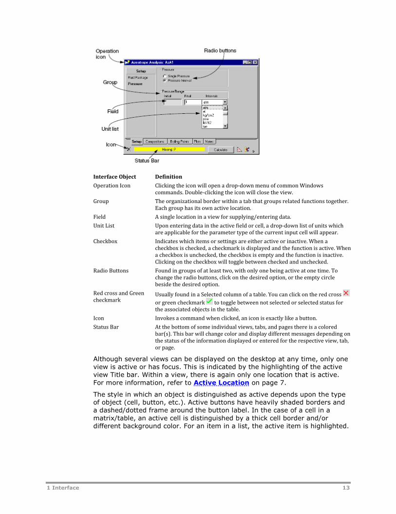
Interface TerminologyThe following figures display some common interface objects in the programviews. The table below each figure list and describes the objects.
Interface Object Definition
Drop-Down List A list of available options under a given menu item, or a list of acceptableresponses to a certain input cell/field.
Minimize icon Reduces the current view into a Minimized view.
Maximize icon Expands the view to its maximum size.
Close icon Closes the view completely.
Matrix / Table Information displayed in a tabular format. Rows of information go across thematrix horizontally, and are organized by variables into different columns, whichrun vertically. The top row of the matrix usually provides a description of theinformation for each column.
For example, a row of information might contain all information about onestream, and one column would contain the inlet temperatures for all streams.
Cell A location in a matrix or table for supplying or viewing information.
Scroll Bar Used to access information which cannot be displayed in the current size of amenu or view.
Scroll Button Part of the Scroll Bar, this object allows you to slide up or down the list. There arealso Scroll Buttons that slide the list left or right.
Button Invokes a command when clicked. Buttons are often used to perform actions,such as deleting or adding or starting calculations. Buttons can also be used toopen up other views.
1 Interface 13
Interface Object Definition
Operation Icon Clicking the icon will open a drop-down menu of common Windowscommands. Double-clicking the icon will close the view.
Group The organizational border within a tab that groups related functions together.Each group has its own active location.
Field A single location in a view for supplying/entering data.
Unit List Upon entering data in the active field or cell, a drop-down list of units whichare applicable for the parameter type of the current input cell will appear.
Checkbox Indicates which items or settings are either active or inactive. When acheckbox is checked, a checkmark is displayed and the function is active. Whena checkbox is unchecked, the checkbox is empty and the function is inactive.Clicking on the checkbox will toggle between checked and unchecked.
Radio Buttons Found in groups of at least two, with only one being active at one time. Tochange the radio buttons, click on the desired option, or the empty circlebeside the desired option.
Red cross and Greencheckmark
Usually found in a Selected column of a table. You can click on the red cross
or green checkmark to toggle between not selected or selected status forthe associated objects in the table.
Icon Invokes a command when clicked, an icon is exactly like a button.
Status Bar At the bottom of some individual views, tabs, and pages there is a coloredbar(s). This bar will change color and display different messages depending onthe status of the information displayed or entered for the respective view, tab,or page.
Although several views can be displayed on the desktop at any time, only oneview is active or has focus. This is indicated by the highlighting of the activeview Title bar. Within a view, there is again only one location that is active.For more information, refer to Active Location on page 7.
The style in which an object is distinguished as active depends upon the typeof object (cell, button, etc.). Active buttons have heavily shaded borders anda dashed/dotted frame around the button label. In the case of a cell in amatrix/table, an active cell is distinguished by a thick cell border and/ordifferent background color. For an item in a list, the active item is highlighted.
14 1 Interface
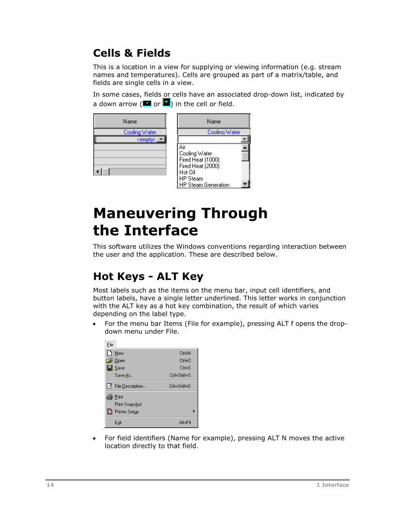
Cells & FieldsThis is a location in a view for supplying or viewing information (e.g. streamnames and temperatures). Cells are grouped as part of a matrix/table, andfields are single cells in a view.
In some cases, fields or cells have an associated drop-down list, indicated by
a down arrow ( or ) in the cell or field.
Maneuvering Throughthe InterfaceThis software utilizes the Windows conventions regarding interaction betweenthe user and the application. These are described below.
Hot Keys - ALT KeyMost labels such as the items on the menu bar, input cell identifiers, andbutton labels, have a single letter underlined. This letter works in conjunctionwith the ALT key as a hot key combination, the result of which variesdepending on the label type.
• For the menu bar Items (File for example), pressing ALT f opens the drop-down menu under File.
• For field identifiers (Name for example), pressing ALT N moves the activelocation directly to that field.

1 Interface 15
• For buttons (Add for example), pressing ALT A invokes the command ofthe button.
The ALT key by itself automatically advances the active location to the firstitem in the menu bar (File). The keyboard arrows move left and right throughthe row, and the down arrow opens the active menu item. If a drop-downmenu has underlined letters, you can invoke the command by using thatletter only. For example, with the File menu open, you can start a new caseby pressing the n key.
The following is a list of all hot key combinations and their related commands,including all ALT key combinations.
Hot Key Combinations Command
ALT E C or CTRL C Clipboard Copy
ALT E P or CTRL V Clipboard Paste
ALT E T or CTRL X Clipboard Cut
ALT F A or CTRL SHIFT S Save Case with another name
ALT F D or CTRL SHIFT D Set Case Description
ESC Cancel previous action
F1 or ALT H C Displays Help Contents
ALT F4 or ALT F X Exit the program
CTRL C or ALT E C Clipboard Copy
CTRL N F N Create a new case
CTRL O or ALT F O Open an existing case
CTRL S or ALT F S Save current case
CTRL V or ALT W P Clipboard Paste
CTRL X or ALT E T Clipboard Cut
CTRL F4 or ALT W C Close current Window
CTRL F6 or ALT W D Send the front window to the back
SHIFT F4 or ALT W E Close all Windows
ALT F H Print a snapshot of the active form
ALT F N or CTRL N Create a new case
ALT F O or CTRL O Open an existing case
ALT F P Print active forms of the Specsheet or Graphic
ALT F S or CTRL S Save current Case
ALT F U G Setup Printer for printing the PFDs, Plots, or Snapshots
ALT F U R Setup Printer for printing Reports, Specsheet, or Text
ALT F X or ALT F4 Exit the program
ALT H A Displays Information about the program
ALT H B Submit or edit Bug Reports
ALT H C or F1 Displays Help Contents
ALT I P Displays Heat Integration Project
ALT I M Displays Heat Integration Manager
ALT I C Displays Heat Integration Case
ALT T P Access to user preferences
ALT T S Access the Script Manager
ALT W C or CTRL F4 Close current Window
ALT W D or CTRL F6 Arrange desktop Windows

16 1 Interface
ALT W E or SHIFT F4 Close all Windows
ALT W I Arrange Icons at bottom of Screen
ALT W L Load a Previously Saved Window Layout (or a Hidden Case)
ALT W S Save Current Window Layout for Future Use
CTRL SHIFT S or ALT F A Save Case with another name
CTRL SHIFT D or ALT F D Set Case Description
CTRL SHIFT F6 Bring the last window to the front
Moving Through a ViewEach cell, field, and button on a view is sequenced. You can move the activelocation using the tab (forward direction), shift tab (reverse direction) keys,or using the mouse pointer.
If the active location is on a cell in a matrix, the tab key will not advance youto the next cell in that matrix, but rather to the next active location in theview (this can be a button or a field).
In some instances, such as input matrix found in the HI Case view, ProcessStreams tab, you will automatically advance to the next input cell when youpress enter.
The active location of the cursor in a view is indicated in one of three ways.
• In the case of a string (e.g. Name field), the entire string in the field willbe reverse highlighted.
• If the cell/field is numerical, another border is placed outside/inside thecell/field border.
• In the case of a button, the perimeter of the button will be highlighted andthe label will be surrounded by a dashed frame.

1 Interface 17
Entering Data
Supplying Input in Cells/Fields
When the required input is a name of an item (e.g., stream, utility, fluidpackage, etc.), you can either supply the input directly via the keyboard, or insome cases (e.g., selecting a Utility Stream name) select the item from adrop-down list of appropriate responses.
If a cell/field allows for selection from a drop-down list, the cell/field willcontain a down arrow at the right side of the cell/field.
If you are supplying the input from the keyboard, (e.g., creating a newstream), click in the cell/field, then enter the text and press enter.
If the input is numerical, the approach is slightly different. When you beginsupplying a number for a numerical cell/field, your input is displayed in thecell/field and the Unit list appears beside the cell/field. The Unit list is like adrop-down list that displays the current default unit for the cell/field property.When you have supplied the number and press enter, the program assumesthat the default unit is the selected unit for the value entered.
If you are supplying the number in a unit other than the default, there aretwo methods available for identifying your unit.
InputMethod
Description
Keyboard Enter a space after the number and then begin typing in the name of the unit. The drop-down list of available units opens, and the entered unit will be highlighted in the drop-down list.
Mouse After supplying the numerical value, but before pressing enter, open the drop-down list
by clicking on the down arrow and select the desired unit from the list.

18 1 Interface
Drop-down Lists and Scroll Bars
Drop-down list provides a list of commands/options to choose as input. Thesecommands/options can be accessed via the mouse, or by keyboard input.Once a drop-down list is opened, maneuvering through the list isaccomplished with the mouse or keyboard.
A drop-down list for a text cell/field can be opened at any time by clicking theappropriate arrow within the cell/field. This opens the drop-down list andmoves the active location to that cell/field. You can also open the drop-downlist for the current active cell/field by pressing the space bar and then thekeyboard down arrow.
For a numerical cell/field, refer to the above Supplying Input in Cells/Fieldssection for information.
Once a drop-down list is opened, you can maneuver through it in severalmethods.
• The most convenient method is via type-matching. Once a drop-down listis opened, keyboard input is interpreted to find the first menu item whichbest matches your input. As you continue to supply input, the matchingcontinues. Pressing enter terminates the string and accepts thehighlighted item. You can also use the keyboard arrow keys to move toany item.
Note: The keyboard Up and Down arrows can be used to move throughthe list. Pressing ENTER selects the highlighted item. The mouse can alsobe used to select the item directly.
• If the menu does not have many items, it appears without scroll bars. Inthis case, you can use the mouse to directly select the desired item, oruse the up and down keyboard arrows to mark the item and then select itwith the enter key.
• In addition, the page up and page down keys move the menu one page,and the home and end keys take you to the first and last item,respectively. The desired item is selected by highlighting it and pressingenter.
• The Scroll Bar/Scroll Button provides similar functionality. Clicking the Upand Down Scroll Arrows advance the menu one item. The scroll button canbe clicked and dragged up and down to quickly scroll the menu. Thedesired item can then be selected by clicking on it.
1 Interface 19
• Clicking the space between the scroll button and the scroll arrow advancesthe menu up or down one page. The desired item can then be selected byclicking on it.
Editing Input
Editing input for a text cell/field can be done in two ways:
• When the cell/field is active, any input you supply will overwrite theprevious input. In some cases, if you want to edit the text and notcompletely overwrite the information, you can click in the active location(the cell or field) again to reposition the cursor.
• You can use the drop-down list to replace the previous input
You have a choice when editing numerical input.
• Click the cell/field to make it the active location, then type in a new valueand press enter. The input is accepted assuming the default units.
• You can change the units of a cell/field by activating the cell/field youwant to change, positioning the cursor at the end of the value andpressing the space bar. You can then either select the new unit from thedrop-down list or typematch the unit.
• Another method is via selective modification. With this route, you place aninsertion point somewhere in the string and make selective changes.
You can use the mouse pointer to make an insertion point somewhere inthe number and make selective changes.
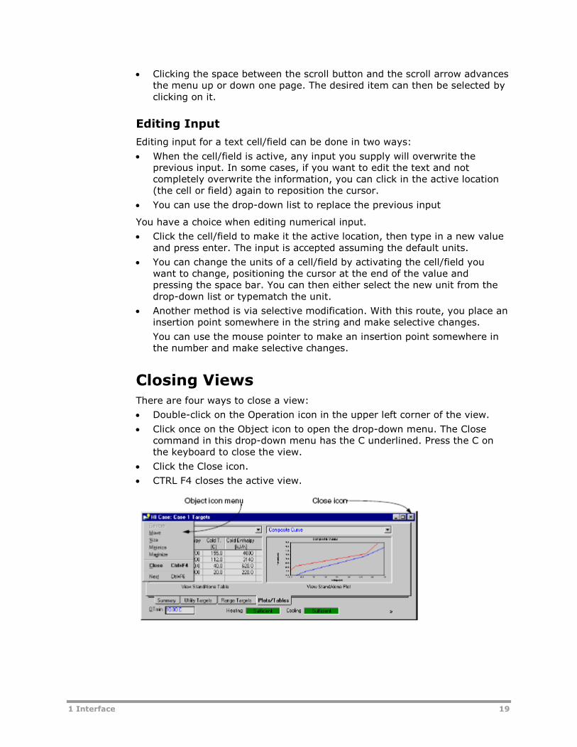
Closing ViewsThere are four ways to close a view:
• Double-click on the Operation icon in the upper left corner of the view.
• Click once on the Object icon to open the drop-down menu. The Closecommand in this drop-down menu has the C underlined. Press the C onthe keyboard to close the view.
• Click the Close icon.
• CTRL F4 closes the active view.

20 1 Interface
Trace WindowAt the bottom of the desktop, there is a window that displays statusmessages and detailed solver information. This window is referred to as theTrace Window. The Trace Window cannot be opened separately.
Opening and Sizing the WindowTo open the Trace Window, position the mouse pointer on any part of theextra thick border directly above the status bar. When the mouse pointer
changes to a sizing arrowhead , click and drag the border vertically.
Available InformationThe Trace Window has three main functions:
• It displays iterative calculations for certain operations. These are shown inblack.
• It displays scripting commands, shown in blue.
• If an operation has an error or warning, but still solves, this message isshown in red.
An example of the contents shown in the Trace Window is displayed in thefigure below. The Trace window has a vertical scroll bar, which allows you tomove through its contents.
Object Inspect MenuYou can access the Object Inspect menu of the Trace Window by placing themouse pointer over the Trace Windows and right-click. The figure belowdisplays the Object Inspect menu.
1 Interface 21
The commands available in the Object Inspect menu for the Trace Windoware:
Command Description
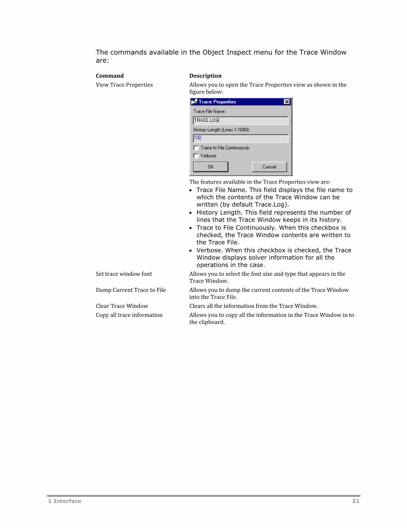
View Trace Properties Allows you to open the Trace Properties view as shown in thefigure below:
The features available in the Trace Properties view are:
• Trace File Name. This field displays the file name towhich the contents of the Trace Window can bewritten (by default Trace.Log).
• History Length. This field represents the number oflines that the Trace Window keeps in its history.
• Trace to File Continuously. When this checkbox ischecked, the Trace Window contents are written tothe Trace File.
• Verbose. When this checkbox is checked, the TraceWindow displays solver information for all theoperations in the case.
Set trace window font Allows you to select the font size and type that appears in theTrace Window.
Dump Current Trace to File Allows you to dump the current contents of the Trace Windowinto the Trace File.
Clear Trace Window Clears all the information from the Trace Window.
Copy all trace information Allows you to copy all the information in the Trace Window in tothe clipboard.

22 1 Interface

2 File Menu Options 23
2 File Menu Options
File MenuThe File menu is the first menu available in the menu bar. The file menucontains most of the commands related to manipulating files and all the printcommands available in the program. The figure below displays the File menu.
You can access the File menu by doing one of the following:
• Move mouse pointer over the File menu in the menu bar and click.
• Press ALT F.
• Press ALT and press the DOWN ARROW key.
If you have previously saved a case in the program, the case name willappear below the Exit command. You can select the case name to open thecase, without using the Open command. The program's quick access to caseoption stores up to five cases.

24 2 File Menu Options
New CommandThe New command creates a new case. If a case is opened when thecommand is selected, you will be prompted to save the current case if therehave been changes since the last save. You can also press CTRL N to accessthe New command.
Note: You can have only one file open at any time. So whenever you create anew case or open a file, the program closes any active case in the programbefore the new case is created or selected file is opened.
To create a new case:
1 Open the File menu and select New.
o If you have an active case that has not been modified since its lastsave, Concept will close the active case.
o If you have an active case that has not been saved, the program willopen a view that prompts you to select one of the three options: savethe case, close the case without saving, or abort creating a new case.
2 After ensuring there are no active cases, the program create a new case.The new case is indicated by the blank desktop and the NoName.hcd inthe title bar.
Note: Alternatively, you can also create a new case by clicking the New Case
icon .

2 File Menu Options 25
Open CommandThe Open command opens an existing case. If a case is open when thecommand is selected, you will be prompted to save the current case if therehave been changes since the last save. You can also press CTRL O to accessthe Open command.
Note: You can have only one file open at any time. So whenever you create anew case or open a file, the program closes any active case in the programbefore the new case is created or selected file is opened.
To open an existing case:
1 Select File-Open from the menu bar.
o If you have an active case that has not been modified since its lastsave, Concept will close the active case.
o If you have an active case that has not been saved, the program willopen a view prompting you to either save the case, close the casewithout saving, or abort creating a new case.
Note: Alternatively, you can also open a case by clicking the Open Case
icon .
2 After ensuring there are no active cases, the program opens the OpenCase view.
3 Select the case you want to open and click the Open button.

26 2 File Menu Options
Save CommandThe Save command saves the active case of the program as a *.hcd file.When saving a case for the first time, use the Save command and supply thefile name and file path. You can also press CTRL S to access the Savecommand.
To save a new case:
1 Open the File menu.
2 Select the Save command.
3 The program will open the Save Case view.
4 You must enter a name for the file in the File name field.You can also select where the file is to be saved using the Save in drop-down list.
Note: The program automatically saved the case in the default file folder.Refer to Locations Page on page 53 for more information regarding thedefault file folder.
5 Click the Save button, when you are done entering the name andselecting the file path. The Save Case view will close, and the program willsave the new case with the appropriate file extension, *.hcd.
If the case has been previously saved, the Save command updates theinformation in the file.
To save a previous case:
1 Open the File menu.
2 Select the Save command.
3 The program will save the active case in the same file path. The existingcase in the disk is replaced with the active case.

2 File Menu Options 27
You can also save a case by clicking the Save Case icon . The Save Caseicon has the same function as the Save command.
Save As CommandThe Save As command saves the active case of the program as a *.hcd file. Ifyou want to change the file name or location of a previously saved case, usethe Save As command. You can also press CTRL SHIFT S to access the SaveAs command.
To save a previous case as a new name or in new file path:
1 Open the File menu.
2 Select the Save As command.
The program will open the Save Case view.
3 You can enter a new name for the file in the File name field. The programautomatically attaches the appropriate file extension, *.hcd.You can also select a different file path for the file using the Save in drop-down list.
The program automatically saved the case in the default file folder. Referto Locations Page on page 53 for more information regarding the defaultfile folder.
28 2 File Menu Options
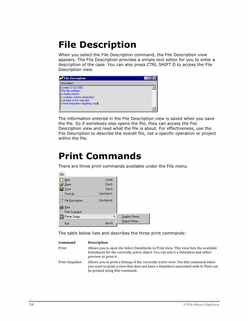
File DescriptionWhen you select the File Description command, the File Description viewappears. The File Description provides a simple text editor for you to enter adescription of the case. You can also press CTRL SHIFT D to access the FileDescription view.
The information entered in the File Description view is saved when you savethe file. So if somebody else opens the file, they can access the FileDescription view and read what the file is about. For effectiveness, use theFile Description to describe the overall file, not a specific operation or projectwithin the file.
Print CommandsThere are three print commands available under the File menu.
The table below lists and describes the three print commands:
Command Description
Print Allows you to open the Select Datablocks to Print view. This view lists the availableDatasheets for the currently active object. You can select a Datasheet and eitherpreview or print it.
Print Snapshot Allows you to print a bitmap of the currently active view. Use this command whenyou want to print a view that does not have a Datasheet associated with it. Plots canbe printed using this command.

2 File Menu Options 29
Printer Setup Opens a sub-menu containing two commands: Graphic Printer and Report Printer.
If you select the Graphic Printer command, the Print Setup view for graphicsappears. The Print Setup view allows you to select the printer, paper orientation,paper size, and source. Use the Graphic Printer command to setup the printer whenprinting plots and snapshots.
If you select the Report Printer command, the Print Setup view for reports appears.The Print Setup view allows you to select the printer, paper orientation, paper size,and source. Use the Report Printer command to setup the printer when printingDatasheets, reports, and text. The Print Setup view varies with different printers.
Printing DatasheetThe Datasheet displays all Worksheet-related information, which can includeinput specifications and calculated results. You can customize the informationdisplayed in the Datasheet on the Select Datablocks to Print view. The list ofavailable datablocks in the Select Datablocks to Print view varies dependingon the selected view.
To access the Select Datablocks to Print view:
1 Select the view containing the information you want to print.
2 Then select the Print from the File menu.
The figure below displays the Select Datablocks to Print view for anAzeotrope Analysis view.
30 2 File Menu Options
The following table lists and describes the object in the Select Datablocks toPrint view:
Object Description
AvailableDatablocks list
Contains all the Worksheets available for the Datasheet of the selected view. Youcan expand the list by clicking the "+" symbols beside the Worksheet, or shrink thelist by clicking the "-" symbols beside the Worksheet.
You can select which Worksheets will appear in the Datasheet by checking orunchecking the corresponding checkboxes in the Available Datablocks group.
Select All button Allows you to check all the Worksheet in the Available Datablocks list, thusinforming the program to include all the Worksheets information into theDatasheet.
Invert Selectionbutton
Allows you to reverse the status of all the checkboxes in the Available Datablocklist. So any checked checkboxes in the list becomes uncheck and vice versa forunchecked checkboxes.
Set Preferencesbutton
Allows you to save the current status of the Worksheet checkboxes in the list as apreference. You can apply the saved preferred selection/preference into otherDatasheets with the same view type.
You can save a preference for the Column Design view, and apply the preferenceto a different Column Design view. However, you cannot apply the preference toan Azeotrope Analysis view.
Use Preferencesbutton
Allows you to apply the saved preference on to the Datasheet of the current view.If no preference was saved, the program default preference setting is applied. Thedefault preference is to include all the available Worksheet into the Datasheet.
Print button Allows you to print a physical copy of the Datasheet using the current setup on theSelect Datablocks to Print view.
Text to Filecheckbox
Check this checkbox to print the Datasheet to an ASCII file.
When this checkbox is checked the Delimited checkbox is made active and theFormat button replaced the Format/Layout button.
Delimitedcheckbox
Check this checkbox to apply the delimiter in the ASCII file.
This checkbox is only available if the Text to File checkbox is checked.
Preview button Allows you to open the Report Preview view. The Report Preview view containsan image of how the printed Datasheet will look like.
Format/Layoutbutton
This button is available when the Text to File checkbox is unchecked. Allows youto open the Session Preferences Format/Layout view. This view allows you tomanipulate the format and layout of the Datasheet.
The view is also the same as the Reports tab, Format / Layout page in the SessionPreference view.
Format button This button is available when the Text to File checkbox is checked. Allows you toopen the Session Preferences Text Format view. This view allows you tomanipulate the format of the Datasheet.
The view is also the same as the Reports tab, Text Format page in the SessionPreference view.
Print Setupbutton
Allows you to open the Print Setup view. This view allows you to select theprinter, the paper orientation, the paper size, and the paper source.

2 File Menu Options 31
Report Preview View
The Report Preview view allows you to see the Datasheet before printing aphysical copy or saving the Datasheet as a text file. The figure below displaysa Report Preview view of a Heat Interrogation case. To access the ReportPreview view, click the Preview button on the Select Datablocks to Print view.
The following table lists and describes the objects available on the ReportPreview view:
Object Icon Description
Format/Layoutbutton
Allows you to open the Session Preferences Format/Layout view. Thisview allows you to manipulate the format and layout of the Datasheet.
The view is also the same as the Reports tab, Format/Layout page in theSession Preference view.
Print Setup button Allows you to open the Print Setup view. This view allows you to selectthe printer, the paper orientation, the paper size, and the paper source.
Update button Allows you to update the information/values on the Datasheet.
Print button Allows you to print the current Datasheet.
Close button Allows you to close the Report Preview view.
Zoom Out icon Allows you to zoom out/away from the Datasheet image.
ZoomFit icon Allows you to resize the width of Datasheet image to fit into the currentview.
Zoom In icon Allows you to zoom in/towards the Datasheet image.
Printing PlotsThere are two methods to print a plot:
• Select the plot view, and then select the Print Snapshot from the Filemenu.

32 2 File Menu Options
• Right-click the plot area and select the Print Plot command from theObject Inspect menu.
Note: For more information about printing plots, refer to the Print Plotsection on page 96.
Exit CommandSelect the Exit command to close and leave the program. You will beprompted to save the current case if any changes occurred since the lastsave. You can also press ALT F4 to access the Exit command.

3 Edit, Managers, & Features Menu Options 33
3 Edit, Managers, & FeaturesMenu Options
Edit MenuThe following commands are available in the Edit menu:
Command Description
Cut Allows you to remove the selected cell(s) from the current view. You can then use thePaste function to place the removed cell(s) in another location or in another application.
Copy Allows you to copy the selected cell(s) to the Clipboard. You can then use the Pastefunction to place the copied cell(s) in another location or in another application.
Paste Allows you to place the copied or cut selections in the location of your choice.
Managers MenuThe Managers menu contains a list of commands to open the Aspen EnergyAnalyzer manager view.
You can access the Managers menu by doing one of the following:
• Move mouse pointer over the Managers menu in the menu bar and click.
• Press alt m.
Aspen Energy AnalyzerIn Aspen Energy Analyzer, the Managers menu contains only one command:
Allows you to open the Heat Integration Manager view. This view managesthe creation, deletion, and modification of the two Heat Integrationoperations: HI Projects and HI Cases.
34 3 Edit, Managers, & Features Menu Options
Features MenuThe Features menu contains a list of commands to open the operation/toolproperty views.
You can access the Features menu by doing one of the following:
• Move mouse pointer over the Features menu in the menu bar and click.
• Press alt f.
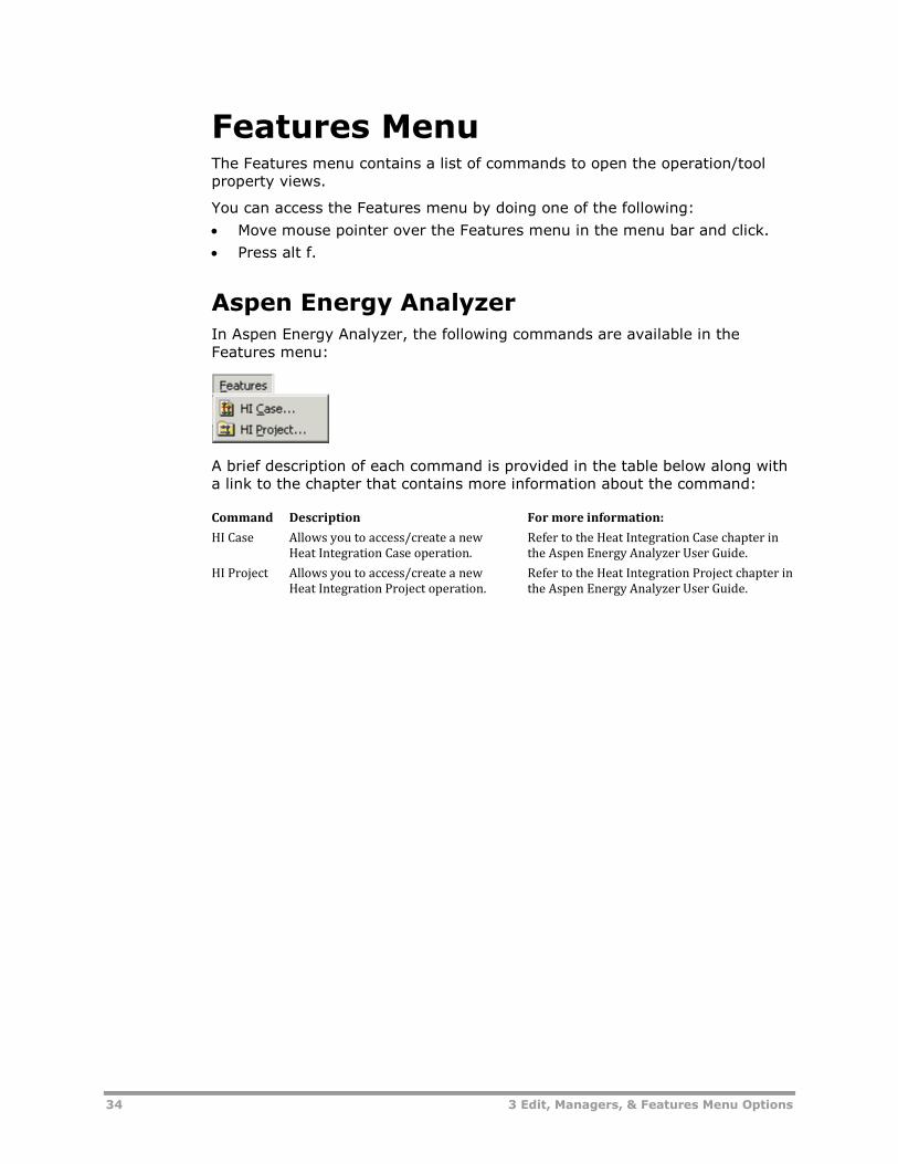
Aspen Energy AnalyzerIn Aspen Energy Analyzer, the following commands are available in theFeatures menu:
A brief description of each command is provided in the table below along witha link to the chapter that contains more information about the command:
Command Description For more information:
HI Case Allows you to access/create a newHeat Integration Case operation.
Refer to the Heat Integration Case chapter inthe Aspen Energy Analyzer User Guide.
HI Project Allows you to access/create a newHeat Integration Project operation.
Refer to the Heat Integration Project chapter inthe Aspen Energy Analyzer User Guide.

4 Tools Menu Options 35
4 Tools Menu Options
Tools MenuYou can access the Tools menu by doing one of the following:
• Move mouse pointer over the Tools menu in the menu bar and click.
• Press alt t.
The following commands are available in the Tools menu:
Command Description
Script Manager Allows you access to the Script Manager.
Macro Language Editor Allows you access to the program's Macro Language Editor view.
Preferences Allows you access to the Session Preferences.

36 4 Tools Menu Options
Script Manager CommandThe Script Manager view is a tool that records all your case interaction, withrespect to all information specified. The recorded script can be played back ata later time. Select the Tools-Script Manager command from the menu bar toopen the Script Manager view.
The following are some important points when using the Script feature:
• Changes made in the Session Preferences are not saved in the script.
• Scripting is always done in the program internal units.
• Scripting is Name specific, so stream and operation names in a script mustbe identical to those in the case in which you are running the script.
• For the playback of a script, the simulation case MUST BE EXACTLY as itwas when the script was recorded, so that the program can perform allthe steps in the script.
RecordingThe procedure for recording a new script is as follows:
1 Save your simulation case. Since the case must be in exactly the samecondition for playback of the recorded script, this is generally a good idea.
2 Open the Tools menu.
3 Select Script Manager. The Script Manager view appears.
4 Select a directory from the Directories list in which the script file will besaved.
5 Click the New button. The program closes the Script Manager view anddisplays the New Script view.

4 Tools Menu Options 37
6 Enter a name in the Name field for the script. If you want, you can alsoenter a description for the script in the Description field.If you did not add an extension to the script file name, the programautomatically adds the *.scp extension.
7 Click the Record button to start recording. The program closes the New
Script view. Notice the red Record icon in the lower right corner of thedesktop.
8 Perform each task that you want to record.
9 When you finish recording commands, open the Script Manager view andclick the Stop Recording button.
If you would like to save the case, DO NOT save it with the same name as instep 1, as this will prevent you from playing back the script.
PlaybackIn order to play a script, the simulation case must be in the same state as itwas prior to the recording of the script. At any time during the playback, youcan stop the script by opening the Script Manager view and clicking the StopPlay button.
Follow this procedure to play a script:
1 Open the case that is associated with the script.
2 Open the Tools menu.
3 Select Script Manager. The Script Manager view appears.
4 Select the script name in the Script Files list. If your script is not listed inthe default directory, you can select a different path in the Directories list.
5 Click the Play button. The program closes the Script Manager view andbegins playing back the script. Notice the green Playback icon in thelower right corner of the desktop.
The steps of the script playback are shown in the Trace Window.
38 4 Tools Menu Options
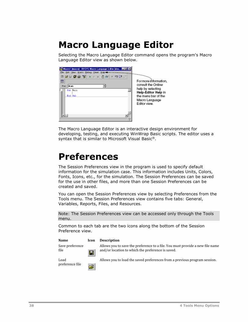
Macro Language EditorSelecting the Macro Language Editor command opens the program's MacroLanguage Editor view as shown below.
The Macro Language Editor is an interactive design environment fordeveloping, testing, and executing WinWrap Basic scripts. The editor uses asyntax that is similar to Microsoft Visual Basic®.
PreferencesThe Session Preferences view in the program is used to specify defaultinformation for the simulation case. This information includes Units, Colors,Fonts, Icons, etc., for the simulation. The Session Preferences can be savedfor the use in other files, and more than one Session Preferences can becreated and saved.
You can open the Session Preferences view by selecting Preferences from theTools menu. The Session Preferences view contains five tabs: General,Variables, Reports, Files, and Resources.
Note: The Session Preferences view can be accessed only through the Toolsmenu.
Common to each tab are the two icons along the bottom of the SessionPreference view.
Name Icon Description
Save preferencefile
Allows you to save the preference to a file. You must provide a new file nameand/or location to which the preference is saved.
Loadpreference file
Allows you to load the saved preferences from a previous program session.

4 Tools Menu Options 39
Saving a Session Preference
To save a preference file:
1 Click the Save preference file icon . The Save Preference File viewappears.
2 Specify the name and location for your preference file.
3 Click the Save button.
Loading a Session Preference
To load a preference file:
1 Click the Load preference file button . The Open Preferences File viewappears.
2 Browse to the location of your preference file (*.prf).
3 Select the file you want to load and click the Open button.
General TabThe General tab shown in the figure below contains three groups: Errors,Show ToolTips, and Data Extraction.
Data Extraction Group
The Data Extraction group allows you to specify the version of the Aspen Plusbackup file you are going to extract information from. For example, thesimulation file that contains the information you want was created in AspenPlus Version 2004. Enter 2004 in the Aspen Plus Version field.

40 4 Tools Menu Options
Errors Group
The Errors group contains two checkboxes which when checked will send thespecified errors to the Trace Window. When these checkboxes are checked,you will not be prompted to acknowledge errors.
Show ToolTips Group
Tooltip is a pop up or fly by that contains information related to an object.The tool tips are displayed by placing the mouse pointer over the associatedobject.
For instance, you can view stream data in the Data tab, Process Streamspage of a HI Case view, by placing the cursor over any cell in the table tomake the tool tip appear.
The Show ToolTips group contains five checkboxes that allows you tocustomize what information appears on the tool tips.
• Show ToolTips. Check this checkbox to display the tool tip for objects thatcontain tool tip information.When the Show ToolTips checkbox is checked, the Use ToolTips checkboxin the Resources tab, Cursors page will also be checked.
• Value in EuroSI Units. Check this checkbox to display the EuroSI units inthe tool tips. Uncheck this checkbox to remove the EuroSI units from thetool tips.
• Value in Field Units. Check this checkbox to display the Field units in thetool tips. Uncheck this checkbox to remove the Field units from the tooltips.
• Value in SI Units. Check this checkbox to display the SI units in the tooltips. Uncheck this checkbox to remove the SI units from the tool tips.
• Value Calculated By. Check this checkbox to display the method ofcalculation in the tool tips. Uncheck this checkbox to remove the methodof calculation units from the tool tips.

4 Tools Menu Options 41
Variables TabThe Variables tab contains two pages: Units and Formats.
Units Page
The Units page allows you to select the unit to use in the current session.
The Unit page contains two groups: Available Unit Sets and Display Units.
The following table contains a list and description of the objects in theAvailable Unit Sets group:
Object Description
Available Unit Sets list Allows you to select the unit set for the current session and contains all theunit sets available in the current session.
Clone button Allows you to clone a default unit set. You can only modify custom unit set.
Delete button Allows you to delete only custom unit sets.
Unit Set Name field Displays the name of the selected unit set. You can only modify names ofthe custom unit sets.

42 4 Tools Menu Options
The following table contains a list and description of the objects in the DisplayUnits group:
Object Description
Display Unitstable
Contains a list of variables and the units associated to the variables. The unitsassociated to the variables changes depending on the unit set selected. You canonly modify the units associated to the variables of a custom unit set.
View button Allows you to see the unit conversion of the selected unit from the Display Unitstable.
Add button Allows you to add a unit conversion for the selected variable from the DisplayUnits table. You can only add new conversion units for the variable of a customunit set.
Delete button Allows you to delete a user added unit conversion from a variable of a custom unitset.
The program has three default unit sets. The default unit sets are: EuroSI,Field, and SI. These three sets are fixed, in which none of the units associatedto the variables can be changed. Since you want to display information inunits other than the default, the program allows you to create your owncustom unit sets.
Note: You cannot delete the program’s default unit sets.
Adding a New Unit Set
You can create the new custom unit sets by cloning an existing set andaltering it. The procedure is as follows:
1 Select the unit set you want to modify from the Available Unit Sets group.
2 Click the Clone button.
The programs clones the selected unit set and automatically gives adefault name to the new unit set. The default name is NewUser.
3 The default name appears in the Available Unit Sets list and in the UnitSet Name field. Notice that the text in the Unit Set Name field is blue incolor, which means you can change the default name.
The units used in the new unit set are the same as the unit set you cloned.

4 Tools Menu Options 43
Change the Unit of a Variable
To the change the units in a unit set:
1 From the list of Available Unit Sets, select the unit set you want to use foryour simulation.
2 In the Displayed Units group, select the unit of the variable you want tochange (e.g., Temperature).
Note: You can not modify the units in any of the three default unit sets:SI, Field, and Euro SI.
3 With the focus in the Temperature unit cell, click the down arrow toopen a drop-down list. The drop-down list shows all available convertibleunits for that unit type.
Note: With the focus in the appropriate cell, you can also press the spacebar to open the drop-down list.
4 From the list, click the unit you want use as your base unit for yoursimulation.
Deleting a Unit Set
To delete a unit set:
1 Select the unit set you want to delete from the list in the Available UnitSets group.
2 Click the Delete button.
Notes:
• You can not delete the three default unit sets: SI, Field, and Euro SI.• You will not be prompted to confirm the deletion of a unit set, so ensure
that you have selected the correct unit set to delete.
Viewing a Unit Conversion
The program performs its calculations in an internal unit set, and every otherunit is converted from these default units. The View button allows you to viewthe conversion factor that the program uses to convert from its internal unit(SI) to the unit chosen in your unit set. You can view the conversion for anyavailable unit.
To view a unit conversion:
1 From the list of Available Unit Sets, select the unit set you want to use foryour simulation.
2 In the Displayed Units group, select the unit for which you want to viewthe conversion.
3 Click the View button to display the Conversion view.

44 4 Tools Menu Options
The Name field displays the name of the unit. The field next to the Namefield displays the conversion factor. Notice that the text in the fields is allblack, indicating that these are View Only fields. You cannot change thecontents in any of the fields.
4 Click the OK or Cancel button to close the view.
Adding a Unit Conversion
If you require a unit that is not available in the program's database, you cancreate your own unit and supply a conversion factor. You can only add a unitto a custom unit set.
To add a unit conversion:
1 From the list of Available Unit Sets, select the custom unit set to whichyou want to add the unit.
2 In the Display Units group, select the unit type you want to add aconversion.
3 Click the Add button. The User Conversion view appears as the figurebelow.
The program’s internal unit is always displayed on the User Conversionview.
4 By default, the program names the new unit UserUnit*. You can changethis name by entering a new name in the Name field.
5 In the second field (the multiply/divide field), type the conversion factorbetween your unit and the program's internal unit.
6 From the drop-down list, specify whether you want to multiply or divide bythe conversion factor.
7 In the final field (the add/subtract field), type the conversion factorbetween your unit and the program's internal unit. To add a factor, specifya value in this field. To subtract, place a negative sign in front of thenumber (e.g., enter -2.0).
8 Click OK and the User Conversion view closes with this unit as the activeunit for that unit type.
4 Tools Menu Options 45
Deleting a Unit Conversion
You can only delete user defined unit conversions. To delete a unitconversion:
1 From the list of Available Unit Sets, select the unit set you want to use foryour simulation.
2 In the Displayed Units group, select a user-created unit you want todelete.
3 Click the Delete button. You will not be prompted to confirm the deletionof the unit. The unit returns to the program's default unit.
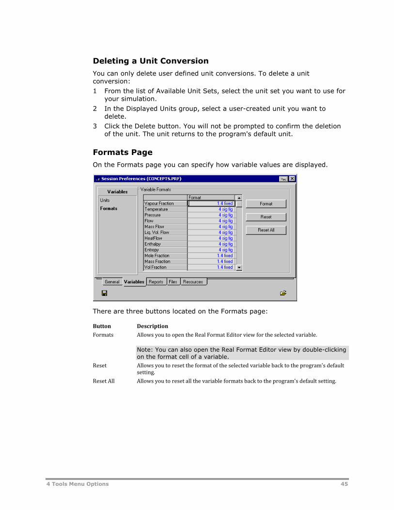
Formats Page
On the Formats page you can specify how variable values are displayed.
There are three buttons located on the Formats page:
Button Description
Formats Allows you to open the Real Format Editor view for the selected variable.
Note: You can also open the Real Format Editor view by double-clickingon the format cell of a variable.
Reset Allows you to reset the format of the selected variable back to the program's defaultsetting.
Reset All Allows you to reset all the variable formats back to the program's default setting.
46 4 Tools Menu Options
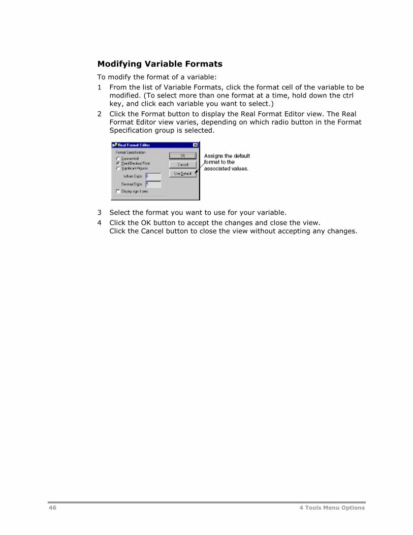
Modifying Variable Formats
To modify the format of a variable:
1 From the list of Variable Formats, click the format cell of the variable to bemodified. (To select more than one format at a time, hold down the ctrlkey, and click each variable you want to select.)
2 Click the Format button to display the Real Format Editor view. The RealFormat Editor view varies, depending on which radio button in the FormatSpecification group is selected.
3 Select the format you want to use for your variable.
4 Click the OK button to accept the changes and close the view.Click the Cancel button to close the view without accepting any changes.

4 Tools Menu Options 47
Real Format Editor View
The Real Format Editor view is used to change variables format in theprogram. The three different formats available are as follows:
Radio Button Description
Exponential Displays the values in scientific notation. The number of significant digitsappearing after the decimal point is set in the Significant Figure field. As anexample:
• Entered or calculated value: 10000.5
• Significant Figure: 5 (includes the first whole digit)
• Final display: 1.0001e+04
Fixed Decimal Point Displays the values in decimal notation. The number of whole digits andsignificant digits appearing after the decimal point are set in the WholeDigits and Decimal Digits fields. As an example:
• Entered or calculated value: 100.5
• Specify whole digits: 3
• Specify decimal digits: 2
• Final display: 100.50
If the entered or calculated value exceeds the specified whole digits, theprogram will display the value as an Exponential, with the sum of thespecified whole and decimal digits being the number of significant figures.
If the Display sign if zero checkbox is checked, the program will display thesign of the number entered or calculated that has been rounded to zero.
Significant Figures Displays the values in either decimal notation or scientific notation. Thenumber of significant digits appearing after the decimal point is set in theSignificant Figure field.
Example 1:
• Entered or calculated value: 100.5
• Significant Figure: 5
• Final display: 100.50
Example 2:
• Entered or calculated value: 10000.5
• Significant Figure: 5
• Final display: 1.0001e+04
48 4 Tools Menu Options
Reports TabThe Reports tab contains four pages: Format/Layout, Text Format,Datasheets, and Company Info.
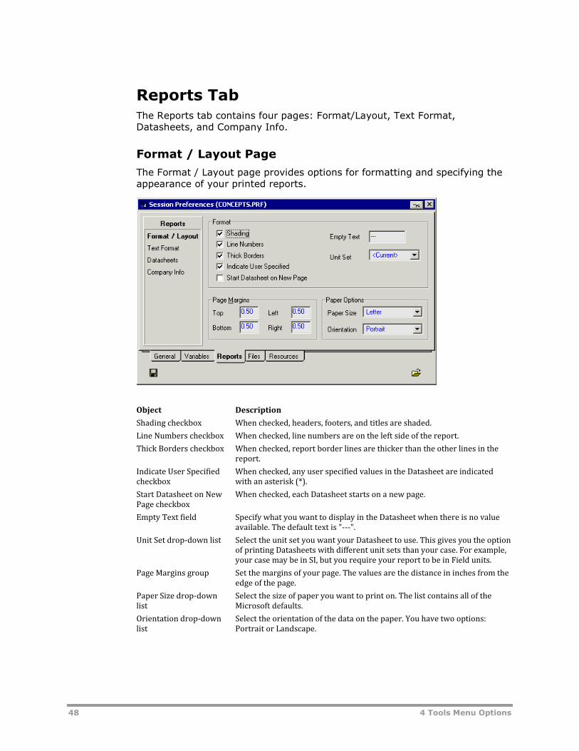
Format / Layout Page
The Format / Layout page provides options for formatting and specifying theappearance of your printed reports.
Object Description
Shading checkbox When checked, headers, footers, and titles are shaded.
Line Numbers checkbox When checked, line numbers are on the left side of the report.
Thick Borders checkbox When checked, report border lines are thicker than the other lines in thereport.
Indicate User Specifiedcheckbox
When checked, any user specified values in the Datasheet are indicatedwith an asterisk (*).
Start Datasheet on NewPage checkbox
When checked, each Datasheet starts on a new page.
Empty Text field Specify what you want to display in the Datasheet when there is no valueavailable. The default text is "---".
Unit Set drop-down list Select the unit set you want your Datasheet to use. This gives you the optionof printing Datasheets with different unit sets than your case. For example,your case may be in SI, but you require your report to be in Field units.
Page Margins group Set the margins of your page. The values are the distance in inches from theedge of the page.
Paper Size drop-downlist
Select the size of paper you want to print on. The list contains all of theMicrosoft defaults.
Orientation drop-downlist
Select the orientation of the data on the paper. You have two options:Portrait or Landscape.

4 Tools Menu Options 49
Text Format Page
For reports printed in text format, the Text Format page allows you to specifysome text formatting options.
Object Description
Use Delimiting By Defaultcheckbox
Check this checkbox if you want the text file to always be delimited.
Title Description Visiblecheckbox
When checked, a title is added to the text file. The title includes the nameof the object and the tabs that are included in the report.
Header Field Visiblecheckbox
When checked, a header is added to the text file. The header includes thecompany information and the date the report was created.
Footer Field Visiblecheckbox
When checked, a footer is added to the text file. The footer includes theprogram version and build number.
Fields Padded forAlignment checkbox
When checked, spaces are added between each field to align the fields.
Empty Text field Specify what you want to display in the Datasheet when there is no valueavailable. The default text is blank.
Delimiter field Specify what you want to use as the delimiter in your text file. The defaulttext is comma delimited (,).

50 4 Tools Menu Options
Datasheets Page
The Datasheets page allows you to select which datablocks are to be includedfor each stream, unit operation, utility, and reaction report printout.
Modifying Datasheets
To modify the datasheets:
1 Select the datasheet type in the Datasheet Types tree.
2 Select the datablocks to be included or excluded in the Default Datablocksgroup.
Note: Click on the “+” or “-” icons to expand or shrink the branches.

4 Tools Menu Options 51
Company Info Page
On the Company Info page, you can provide some information about yourcompany, such as the company name, location, and logo.
Note: The program does not automatically resize a bitmap file to fit the logobox on this page. The maximum logo size that can be accommodated by thelogo box is 6.55 cm wide by 2.38 cm high.
To modify the company information:
1 In the Company Name field, type the company name that you want todisplay in the report header.
2 In the Company Location text editor, type the company location that youwant to display in the report header.
3 To add a company logo, click the Select button. The Select Bitmap on Diskview appears. Browse to the location of your bitmap file (*.bmp).
The logo picture has to be in bitmap format.
4 Select the file you want to import and click the Open button.

52 4 Tools Menu Options
Files TabThe Files tab contains two pages: Options and Locations.
Options Page
The Options page allows you to modify the preferences used when saving oropening a case.
From the Select style for `File Open' and `Save As' dialogs group, click eitherthe Win 95/NT common dialogs or the HYPROTECH file picker radio button.The HYPROTECH file picker displays custom The program's open and saveviews that show the build in which the case was saved, and the casedescription (if one was added).
In the AutoRecovery Settings and Backups group, use the checkboxes toselect the options you want to use. The following options are available:
Object Description
Save AutoRecovery CasesEvery
When checked, the program saves an auto recovery case every specifiedamount of time. Use the minutes field to specify the amount of timebetween every save. You can use the up and down arrows to increaseand decrease the value of the field by one with each click, or you canenter a value directly in the field.
Save AutoRecovery CaseWhile Integrating checkbox
When checked, the program saves an auto recovery case every time theintegrator is run. This checkbox is only available when the SaveAutoRecovery Cases Every checkbox is checked.
Number of Case BackupsAutomatically Maintainedfield
This field is used in conjunction with the Number of Case BackupsAutomatically Maintained. When the field is specified with a number,the program maintains the specified number of backups of eachsimulation, using the extension bk*. The newest backup is bk0, the nextnewest bk1, etc.
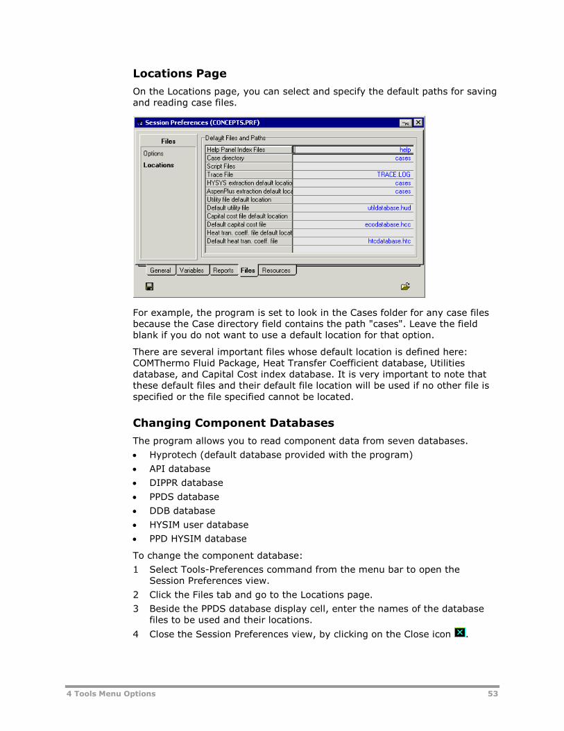
4 Tools Menu Options 53
Locations Page
On the Locations page, you can select and specify the default paths for savingand reading case files.
For example, the program is set to look in the Cases folder for any case filesbecause the Case directory field contains the path "cases". Leave the fieldblank if you do not want to use a default location for that option.
There are several important files whose default location is defined here:COMThermo Fluid Package, Heat Transfer Coefficient database, Utilitiesdatabase, and Capital Cost index database. It is very important to note thatthese default files and their default file location will be used if no other file isspecified or the file specified cannot be located.
Changing Component Databases
The program allows you to read component data from seven databases.
• Hyprotech (default database provided with the program)
• API database
• DIPPR database
• PPDS database
• DDB database
• HYSIM user database
• PPD HYSIM database
To change the component database:
1 Select Tools-Preferences command from the menu bar to open theSession Preferences view.
2 Click the Files tab and go to the Locations page.
3 Beside the PPDS database display cell, enter the names of the databasefiles to be used and their locations.
4 Close the Session Preferences view, by clicking on the Close icon .
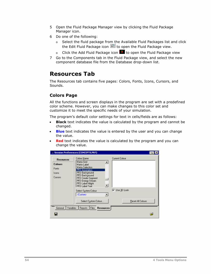
54 4 Tools Menu Options
5 Open the Fluid Package Manager view by clicking the Fluid PackageManager icon.
6 Do one of the following:
o Select the fluid package from the Available Fluid Packages list and click
the Edit Fluid Package icon to open the Fluid Package view.
o Click the Add Fluid Package icon to open the Fluid Package view
7 Go to the Components tab in the Fluid Package view, and select the newcomponent database file from the Database drop-down list.
Resources TabThe Resources tab contains five pages: Colors, Fonts, Icons, Cursors, andSounds.
Colors Page
All the functions and screen displays in the program are set with a predefinedcolor scheme. However, you can make changes to this color set andcustomize it to meet the specific needs of your simulation.
The program’s default color settings for text in cells/fields are as follows:
• Black text indicates the value is calculated by the program and cannot bechanged.
• Blue text indicates the value is entered by the user and you can changethe value.
• Red text indicates the value is calculated by the program and you canchange the value.

4 Tools Menu Options 55
The following table contains a list and description of the objects in the ColorsPage view:
Object Description
Color Name list Contains all the screen elements in the program for which you canchange the color.
Current Color selector Displays the current color for the selected program element in the ColorName list.
Select System Color drop-down list
This drop-down list contains the color system applied to the selectedelement in the Color Name list.
Select Custom Color button Allows you to open the Color Palette. The Color Palette is used to selecta different color or supply a custom color.
You can double-click in the Current Color selector to open the ColorPalette.
Use 3D Look checkbox Check or Uncheck this checkbox to toggle the 3-dimensional appearanceof views when using Windows 2000/XP.
Reset All Colors button Allows you to reset all element colors to the program's default colorscheme.
To change the color of an element:
1 Select the item from the Color Name list.
2 From the Select System Color drop-down list, select one of the systemcolors that are available or select <Custom>.
3 If you select <Custom>, click the Select Custom Color button. The ColorPalette appears.
4 Select the color you want from the Color Palette or your own customizecolor and click the OK button.
5 Notice the selected item has changed from the default color to the newcolor you selected. You can continue to change whatever item colors youwant.
Note: If you change any color settings and then want to return to the defaultprogram colors, click the Reset All Colors button.

56 4 Tools Menu Options
Fonts Page
All the text appearing in the program has a predefined font scheme. However,like the color scheme, you are able to change the font scheme. The structureof the Fonts page is much like the Colors page, as shown in the figure below.
The following table contains a list and description of the objects on the Fontspage:
Object Description
Font Name list Contains all the text items in Concept.
Current Fontselector
Displays the current font for the selected item in the Font Name list.
Select System Fontfield
Displays the system font currently applied to the selected font. You can selectanother system font in the drop-down list.
Select Custom Fontbutton
Allows you to open the Font view.
You can also double-click in the Current Font selector to open the Font view.
Test Scaling field This field is used for scaling the font in the Current Font field. The defaultdisplay scale value is 1.0. You can change the number value in this field.Increasing the number increases the size of the font, and decreasing the numberdecreases the font size in the Current Font field.
Reset All Fontsbutton
Allows you to reset all fonts to the program's default font scheme.

4 Tools Menu Options 57
Font View
The Font view allows you to change the font type, style, and size of theselected text item in the Font Name list on the Fonts page.
To change the font for a text item:
1 Select the text item in the Font Name list.
2 From the Select System Font drop-down list, select one of the systemfonts that are available or select <Custom>.
3 If you selected <Custom>, click the Select Custom Font button. The Fontview appears so you can select the font you want.
4 Click the OK button to return to the Preferences Fonts page. The new fontappears in the Current Font field.
Icons Page
The program has a default icon scheme. Any icons in the program that youcan change are displayed on the Icons page. The structure of the Icons pageis the same as the Colors and Fonts pages.
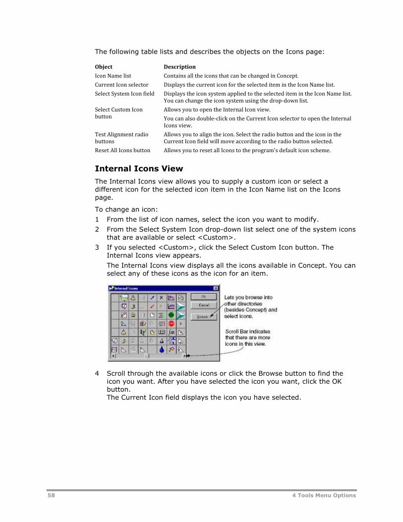
58 4 Tools Menu Options
The following table lists and describes the objects on the Icons page:
Object Description
Icon Name list Contains all the icons that can be changed in Concept.
Current Icon selector Displays the current icon for the selected item in the Icon Name list.
Select System Icon field Displays the icon system applied to the selected item in the Icon Name list.You can change the icon system using the drop-down list.
Select Custom Iconbutton
Allows you to open the Internal Icon view.
You can also double-click on the Current Icon selector to open the InternalIcons view.
Test Alignment radiobuttons
Allows you to align the icon. Select the radio button and the icon in theCurrent Icon field will move according to the radio button selected.
Reset All Icons button Allows you to reset all Icons to the program's default icon scheme.
Internal Icons View
The Internal Icons view allows you to supply a custom icon or select adifferent icon for the selected icon item in the Icon Name list on the Iconspage.
To change an icon:
1 From the list of icon names, select the icon you want to modify.
2 From the Select System Icon drop-down list select one of the system iconsthat are available or select <Custom>.
3 If you selected <Custom>, click the Select Custom Icon button. TheInternal Icons view appears.
The Internal Icons view displays all the icons available in Concept. You canselect any of these icons as the icon for an item.
4 Scroll through the available icons or click the Browse button to find theicon you want. After you have selected the icon you want, click the OKbutton.The Current Icon field displays the icon you have selected.

4 Tools Menu Options 59
Cursors Page
As with the Colors, Fonts, and Icons pages, the program allows you tocustomize the mouse pointers. Cursors type is often specific to certainfunctions. Any cursor types that you can change are displayed on the Cursorspage.
The following table lists and describes the objects on the Cursors page:
Object Description
Cursor Name list Displays all the cursors available in Concept.
Current Cursor selector Place the mouse pointer on this display field to display the current cursorfor the selected item in the Cursor Name list.
Select System Cursor field Displays the cursor system presently applied to the selected item in theCursor Name list. You can change the cursor system using the drop-downlist.
Select Custom Cursorbutton
Allows you to open the Internal Cursors view.
You can also double-click in the Current Cursor selector to open theInternal Cursors view.
Use Tool Tips checkbox When checked, certain objects in the view will display the tool tips whenthe mouse pointer hovers over the object.
When unchecking the Use ToolTips checkbox, the Show ToolTipscheckbox in the General tab will also be unchecked.
Reset All Cursors button Allows you to reset all cursors to the program's default cursor scheme.

60 4 Tools Menu Options
Internal Cursors View
The Internal Cursors view allows you to change the cursor for the selectedcursor item in the Cursor Name list on the Cursors page.
To change a cursor:
1 From the list of cursor names, select the cursor you want to modify.
2 From the Select System Cursor drop-down list, select one of the systemcursors that are available or select <Custom>.
3 If you selected <Custom>, click the Select Custom Cursor button. TheInternal Cursors view appears so you can select the cursor you want.
4 After selecting the icon you want from the list on the Internal Cursorsview, click the OK button.The Current Cursor field will display the cursor you selected, if you placedthe mouse pointer over the field.

5 Window & Help Menu Options 61
5 Window & Help MenuOptions
Window MenuThe Window menu contains general Windows application functions. Theoptions include:
Command Description
Arrange Desktop Cascades all views which are currently open and not iconized.
Arrange Icons Arranges iconized views horizontally at the bottom of the desktop.
Close ctrl+f4 Closes the active view.
Close All Closes all the views.
Save Workspace Allows you to save the current desktop layout for future use.
Load Workspace Allows you to load another case which is currently open. This function lets youtoggle between cases.
The last group of commands in this menu is a list of all open views on thedesktop. The active view is indicated with a black checkmark .
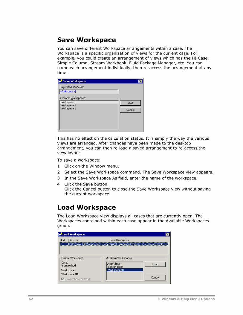
62 5 Window & Help Menu Options
Save WorkspaceYou can save different Workspace arrangements within a case. TheWorkspace is a specific organization of views for the current case. Forexample, you could create an arrangement of views which has the HI Case,Simple Column, Stream Workbook, Fluid Package Manager, etc. You canname each arrangement individually, then re-access the arrangement at anytime.
This has no effect on the calculation status. It is simply the way the variousviews are arranged. After changes have been made to the desktoparrangement, you can then re-load a saved arrangement to re-access theview layout.
To save a workspace:
1 Click on the Window menu.
2 Select the Save Workspace command. The Save Workspace view appears.
3 In the Save Workspace As field, enter the name of the workspace.
4 Click the Save button.Click the Cancel button to close the Save Workspace view without savingthe current workspace.
Load WorkspaceThe Load Workspace view displays all cases that are currently open. TheWorkspaces contained within each case appear in the Available Workspacesgroup.
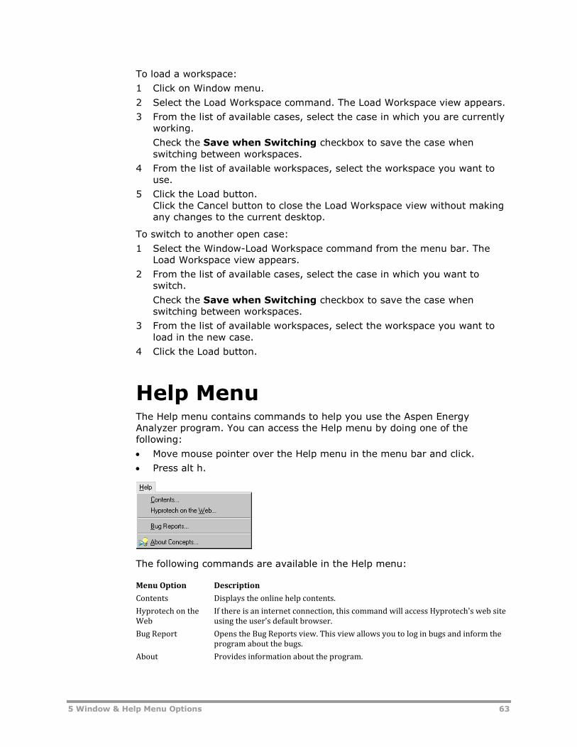
5 Window & Help Menu Options 63
To load a workspace:
1 Click on Window menu.
2 Select the Load Workspace command. The Load Workspace view appears.
3 From the list of available cases, select the case in which you are currentlyworking.
Check the Save when Switching checkbox to save the case whenswitching between workspaces.
4 From the list of available workspaces, select the workspace you want touse.
5 Click the Load button.Click the Cancel button to close the Load Workspace view without makingany changes to the current desktop.
To switch to another open case:
1 Select the Window-Load Workspace command from the menu bar. TheLoad Workspace view appears.
2 From the list of available cases, select the case in which you want toswitch.
Check the Save when Switching checkbox to save the case whenswitching between workspaces.
3 From the list of available workspaces, select the workspace you want toload in the new case.
4 Click the Load button.
Help MenuThe Help menu contains commands to help you use the Aspen EnergyAnalyzer program. You can access the Help menu by doing one of thefollowing:
• Move mouse pointer over the Help menu in the menu bar and click.
• Press alt h.
The following commands are available in the Help menu:
Menu Option Description
Contents Displays the online help contents.
Hyprotech on theWeb
If there is an internet connection, this command will access Hyprotech's web siteusing the user's default browser.
Bug Report Opens the Bug Reports view. This view allows you to log in bugs and inform theprogram about the bugs.
About Provides information about the program.

64 5 Window & Help Menu Options
Adding a Bug ReportTo add a bug report:
1 Open the Help menu and select Bug Reports command. The Bug Reportsview appears.
2 Click the New button on the Bug Reports view, to display the Bug Reportview.
3 In the Bug Title field, type the name of the bug report.
4 The current date and time appear in the Date field, but you can change itif necessary.
5 In the Reported by field, type a contact name so Technical Support canask further questions or provide answers to the problem.
6 In the Class group, select either the Bug or Enhancement radio button.
7 In the Priority group, select either the High, Medium or Low radio button.
8 In the Program Area field, enter the area of the program in which the bugis found. For example, if a bug is found on the Plots tab of the Phase

5 Window & Help Menu Options 65
Equilibrium view, specify Plots tab - Phase Equilibrium operation. Be asspecific as possible so the problem can be located.
9 In the Step-by-Step Description text editor, enter the steps used toproduce the bug. Be as specific as possible so the problem can be locatedand fixed.
10 In the Reproducibility group, click either the Always, Sometimes, or Neverradio button.
11 Click the Write button to display the Save File view.
12 Specify a name and location for your bug report file.
13 Click the Save button.
14 E-mail the bug report file to the AspenTech Support Center [email protected].
Editing a Bug ReportTo edit a bug report:
1 Open the Help menu and select Bug Reports command. The Bug Reportsview appears.
2 From the list of available bug reports, select the bug report you want edit.
3 Click the Edit button to display the Bug Report view.
4 From this view, modify any of the parameters making up the bug report.
Deleting a Bug ReportTo delete a bug report:
1 Open the Help menu and click Bug Reports. The Bug Reports viewappears.
2 From the list of available bug reports, select the bug report you wantdelete.
3 Click the Delete button.
Note: You will not be prompted to confirm the deletion of a bug report, soensure the correct report is selected before deleting.

66 5 Window & Help Menu Options
6 Object Inspect Menu 67
6 Object Inspect Menu
Object Inspect MenuIn the program, there are a number of instances in which either the mouse orthe keyboard can be used. You can perform many of the tasks andmanipulations by using the Object Inspect menu. Place the mouse pointerover the object you want to inspect and right-click to open the Object Inspectmenu of the object. Different Object Inspect menus appear depending uponthe object selected (i.e., Stream, Plot, Operation, etc.).
Empty Area in a ViewIf you right-click an empty space in a view containing a table and tabs orpages, an Object Inspect menu appears.
Command Description
Print Datasheet Lists the available Datasheets for the currently active object. You can highlight aDatasheet and either preview or print it. Refer to Print Commands on page 28for more details.
Open Page Opens a new view that displays only the active page information. The Open Pagecommand is not available in all Object Inspect menus.
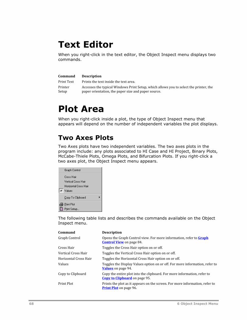
68 6 Object Inspect Menu
Text EditorWhen you right-click in the text editor, the Object Inspect menu displays twocommands.
Command Description
Print Text Prints the text inside the text area.
PrinterSetup
Accesses the typical Windows Print Setup, which allows you to select the printer, thepaper orientation, the paper size and paper source.
Plot AreaWhen you right-click inside a plot, the type of Object Inspect menu thatappears will depend on the number of independent variables the plot displays.
Two Axes PlotsTwo Axes plots have two independent variables. The two axes plots in theprogram include: any plots associated to HI Case and HI Project, Binary Plots,McCabe-Thiele Plots, Omega Plots, and Bifurcation Plots. If you right-click atwo axes plot, the Object Inspect menu appears.
The following table lists and describes the commands available on the ObjectInspect menu.
Command Description
Graph Control Opens the Graph Control view. For more information, refer to GraphControl View on page 84.
Cross Hair Toggles the Cross Hair option on or off.
Vertical Cross Hair Toggles the Vertical Cross Hair option on or off.
Horizontal Cross Hair Toggles the Horizontal Cross Hair option on or off.
Values Toggles the Display Values option on or off. For more information, refer toValues on page 94.
Copy to Clipboard Copy the entire plot into the clipboard. For more information, refer toCopy to Clipboard on page 95.
Print Plot Prints the plot as it appears on the screen. For more information, refer toPrint Plot on page 96.

6 Object Inspect Menu 69
Printer Setup Accesses the typical Windows Print Setup, which allows you to select theprinter, the paper orientation, the paper size and paper source.
Triangle PlotsTriangle plots have three independent variables. The triangle plots in theprogram include: Ternary Plots, Component Space Plots, and RCM Plots andSketches. If you right-click a Component Space plot, the Object Inspect menuappears.
Depending on the plot, none or one of the two following commands mayappear above the Plot Orientation command.
• Calculate. Performs all calculations and updates the plot. Available only onRCM Plots.
• Show Entire Profiles/Show Profiles to Intersection. Show stripping,rectifying, and intermediate profiles until they reach a pinch point or untilthey intersect. Available only on Component Space Plots.
The following table lists and describes the rest of the commands available onthe Object Inspect menu.
Command Description
Plot Orientation Opens the Plot Orientation view. For more information, refer to PlotOrientation View on page 97.
Graph Control Opens the Graph Control view. For more information, refer to Graph ControlView on page 84.
Zoom Out Zooms display out by 25%.
Values Toggles on or off the fly by displaying pointed curve coordinates. For moreinformation, refer to Values on page 94.
Equilateral/RightAngle
Toggles the type of triangle plot displayed as Equilateral or Right Angle.
Copy to Clipboard Copy the entire plot into the clipboard. For more information, refer to Copy toClipboard on page 95.
Print Plot Prints the plot as it appears on the screen. For more information, refer to PrintPlot on page 96.
Printer Setup Accesses the typical Windows Print Setup, which allows you to select theprinter, the paper orientation, the paper size and paper source.
Quaternary PlotsQuaternary plots have four independent variables. A four-component RCMplot in the program is an example of a quaternary plot. If you right-click aquaternary plot, the Object Inspect menu appears.

70 6 Object Inspect Menu
Command Description
Rotation Toggles on or off the rotation control of the plot.
When the rotation control is enabled, you can manipulate the angle of the displayedquaternary plot by clicking and dragging the mouse pointer within the plot orpressing the arrow keys.
Border Toggles on or off the border of the quaternary plot.
Lines Toggles on or off the residue curves in the quaternary plot.
Trace Toggles whether the X-Y, Y-Z, and X-Z planes appear near the quaternary plot.
Values Toggles on or off the fly by displaying pointed curve coordinates. For moreinformation, refer to Values on page 94.
Copy ToClipboard
Copy the entire plot into the clipboard. For more information, refer to Copy toClipboard on page 95.
Print Plot Prints the plot as it appears on the screen. For more information, refer to Print Ploton page 96.
Printer Setup Accesses the typical Windows Print Setup, which allows you to select the printer, thepaper orientation, the paper size and paper source.
The commands in the following table apply to the quaternary plot of theProperty Table operation:
Command Description
Graph Control Opens the Graph Control view. For more information, refer to Graph ControlView on page 84.
Color Control Opens the Color Editor view.
Show Plane Opens the View view. The View view contains a binary plot of an active plane cut(indicated by thick black plot line). If there is no active plane cut on the plot, thebinary plot appears blank.
Plane Cutting Toggles on or off the plane cutting option.
When the plane cutting option is on, you can cut a plane by clicking and dragging
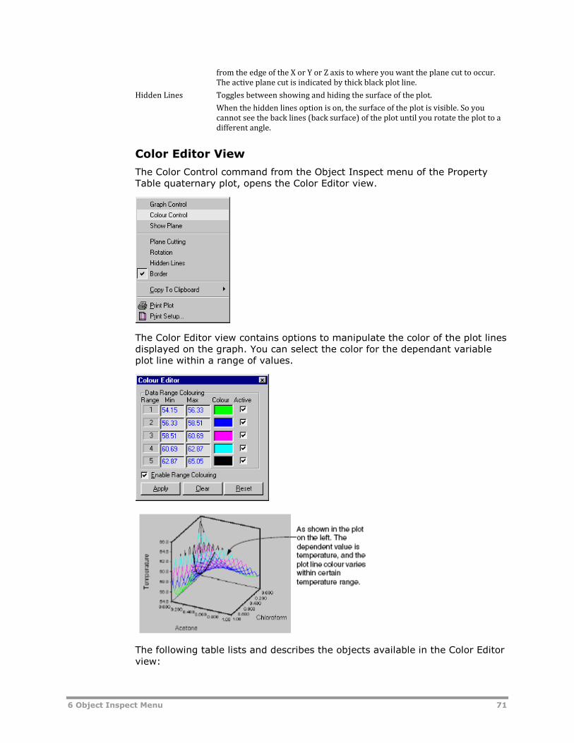
6 Object Inspect Menu 71
from the edge of the X or Y or Z axis to where you want the plane cut to occur.The active plane cut is indicated by thick black plot line.
Hidden Lines Toggles between showing and hiding the surface of the plot.
When the hidden lines option is on, the surface of the plot is visible. So youcannot see the back lines (back surface) of the plot until you rotate the plot to adifferent angle.
Color Editor View
The Color Control command from the Object Inspect menu of the PropertyTable quaternary plot, opens the Color Editor view.
The Color Editor view contains options to manipulate the color of the plot linesdisplayed on the graph. You can select the color for the dependant variableplot line within a range of values.
The following table lists and describes the objects available in the Color Editorview:

72 6 Object Inspect Menu
Object Description
Range cell Displays the designated number for the different color range. You can haveup to five different color range.
Min cell Allows you to specify the minimum value when the selected color shouldappear on the plot.
Max cell Allows you to specify the maximum value when the selected color shouldappear on the plot.
Color cell Allows you to select the color that will appear for the selected value range.
To change the color of a value range:
1 Double-click in the Color cell. The Color Palette appears.
2 Select the color you want from the Color Palette or yourown customize color and click the OK button.
Active checkbox Allows you to toggle on or off the selected color in the plot for the specifiedrange.
Enable Range Coloringcheckbox
Allows you to toggle on or off the different color of the specified valuerange.
• If the checkbox is unchecked, the plot lines on the graph isblue in color.
• If the checkbox is checked, the plot lines on the graphdisplays the color of the specified value range.
Apply button Allows you to apply any changes you make on the Color Editor view to thecurrent plot.
Clear button Allows you to clear all the options/selections in the Data Range Coloringgroup.
Reset button Allows you to reset all the options/selections in the Data Range Coloringgroup to the program default selections.

6 Object Inspect Menu 73
Project ViewIn any project view, there are three different panes and two or three differentlevels. Depending on the level, the pane, and the area on which you right-clicked, the Object Inspect menu will be different.
Viewer PaneAt any level, right-clicking in an empty space in the Viewer pane will open theObject Inspect menu shown on the left. An empty space of a view is definedas any area outside a list, text editor, plot, HEN diagram, or PFD. Thefollowing table contains a list and description of the commands in the ObjectInspect menu.
Command Description
MaximizeFrame
Maximizes the selected pane so that it is the only one visible in the project view.
When viewing a maximized pane, you can still access the other two panes by clickingand dragging the double border now situated at the pane edges.
Open Frame Opens a new view that displays only the selected pane.
Reset Frame Restores the selected pane to default size.
Viewer Group
The Viewer group contains four different Object Inspect menu, depending onthe active level and type of operation selected.
Note: You have to right-click within the Viewer group list to access theseObject Inspect menus.
Project Level
For any operation at the project level, right-clicking in the Viewer group listopens the Object Inspect menu shown on the left. The commands in themenu are described in the table below.
Command Description

74 6 Object Inspect Menu
Add a Scenario Adds a scenario under the selected project level.
Rename Project Renames the selected project
Scenario Level
There are three operations in the program that uses the project view: ColumnSequencing, Azeotropic Column Sequencing, and HI Project.
Azeotropic Column Sequencing & Column Sequencing
For Azeotropic Column Sequencing and Column Sequencing operations, right-clicking in the Viewer group list opens the Object Inspect menu shown on theleft. The commands in the menu are described in the table below.
Command Description
Clone Scenario Clones the selected scenario.
Rename Scenario Renames the selected scenario.
Delete Scenario Deletes the selected scenario.
HI Project
For the HI Project operation, right-clicking in the Viewer group list opens theObject Inspect menu shown on the left. The commands in the menu aredescribed in the table below.
Command Description
Add Design Adds a design under the selected scenario.
Copy Scenario Data Allows you to select the data that you want to copy to an existingscenario. This is useful in copying only part of the input data to a newlycreated scenario.
Clone Scenario Generates a complete copy of the selected scenario.
Delete Scenario Removes the selected scenario.
Rename Scenario Rename the selected scenario
Extract Data From HYSYS Generates heat integration data from an existing case in HYSYS or AspenPlus.

6 Object Inspect Menu 75
Recommend Design Automatically generates a heat exchanger network from the scenarioinformation.
Enter Retrofit Mode Allows you to take the selected scenario into Retrofit mode.
Design Level
As mentioned before, there are three operations that uses the project view:Column Sequencing, Azeotropic Column Sequencing, and HI Project.
Azeotropic Column Sequencing & Column Sequencing
For Azeotropic Column Sequencing and Column Sequencing operations, right-clicking in the Viewer group list opens the Object Inspect menu shown on theleft. The commands in the menu are described in the table below.
Command Description
Delete Design Removes the selected design.
Clone Design Generates a copy of the selected design
Rename Design Renames the selected design
Optimize ColumnPressures
Opens the Optimize Pressure view.
The Optimize Pressure view allows you to specify the pressure range andthe maximum number of iterations for the optimize calculations. Refer tothe Optimizing Column Pressure from the Aspen Energy AnalyzerReference Guide for more information.
HI Project
For the HI Project operation, right-clicking in the Viewer group list opens theObject Inspect menu shown on the left. The commands in the menu aredescribed in the table below.
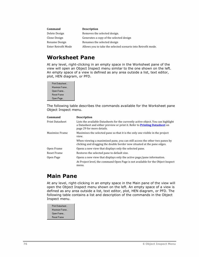
76 6 Object Inspect Menu
Command Description
Delete Design Removes the selected design.
Clone Design Generates a copy of the selected design
Rename Design Renames the selected design
Enter Retrofit Mode Allows you to take the selected scenario into Retrofit mode.
Worksheet PaneAt any level, right-clicking in an empty space in the Worksheet pane of theview will open an Object Inspect menu similar to the one shown on the left.An empty space of a view is defined as any area outside a list, text editor,plot, HEN diagram, or PFD.
The following table describes the commands available for the Worksheet paneObject Inspect menu.
Command Description
Print Datasheet Lists the available Datasheets for the currently active object. You can highlighta Datasheet and either preview or print it. Refer to Printing Datasheet onpage 29 for more details.
Maximize Frame Maximizes the selected pane so that it is the only one visible in the projectview.
When viewing a maximized pane, you can still access the other two panes byclicking and dragging the double border now situated at the pane edges.
Open Frame Opens a new view that displays only the selected pane.
Reset Frame Restores the selected pane to default size.
Open Page Opens a new view that displays only the active page/pane information.
At Project level, the command Open Page is not available for the Object Inspectmenu.
Main PaneAt any level, right-clicking in an empty space in the Main pane of the view willopen the Object Inspect menu shown on the left. An empty space of a view isdefined as any area outside a list, text editor, plot, HEN diagram, or PFD. Thefollowing table contains a list and description of the commands in the ObjectInspect menu.

6 Object Inspect Menu 77
Command Description
Print Datasheet Lists the available Datasheets for the currently active object. You can highlighta Datasheet and either preview or print it. Refer to Printing Datasheet onpage 29 for more details.
Maximize Frame Maximizes the selected pane so that it is the only one visible in the projectview.
When viewing a maximized pane, you can still access the other two panes byclicking and dragging the double border now situated at the pane edges.
Open Frame Opens a new view that displays only the selected pane.
Reset Frame Restores the selected pane to default size.
PFDThe Column Sequencing view displays Process Flow Diagrams (PFD) ofvarious feasible column sequences in the Main pane at the Design level. Whenyou right-click on the PFD, the Object Inspect menu appears.
Command Description
Copy toClipboard
Copy the entire PFD view into the clipboard. For more information, refer to Copy toClipboard on page 95.
Print Plot Prints the plot as it appears on the screen. For more information, refer to Print Ploton page 96.
Printer Setup Accesses the typical Windows Print Setup, which allows you to select the printer, thepaper orientation, the paper size and paper source.
Grid DiagramThe heat exchanger network (HEN) design is graphically displayed in the GridDiagram. The Grid Diagram is located in different areas for differentoperation:
• In HI Project operation: the HI Project view, Main pane at the Designlevel.
• In HI Case operation: the HEN Design view, Grid Diagram tab.
When you right-click the HEN design, the Object Inspect menu appearssimilar to the figure on the left.
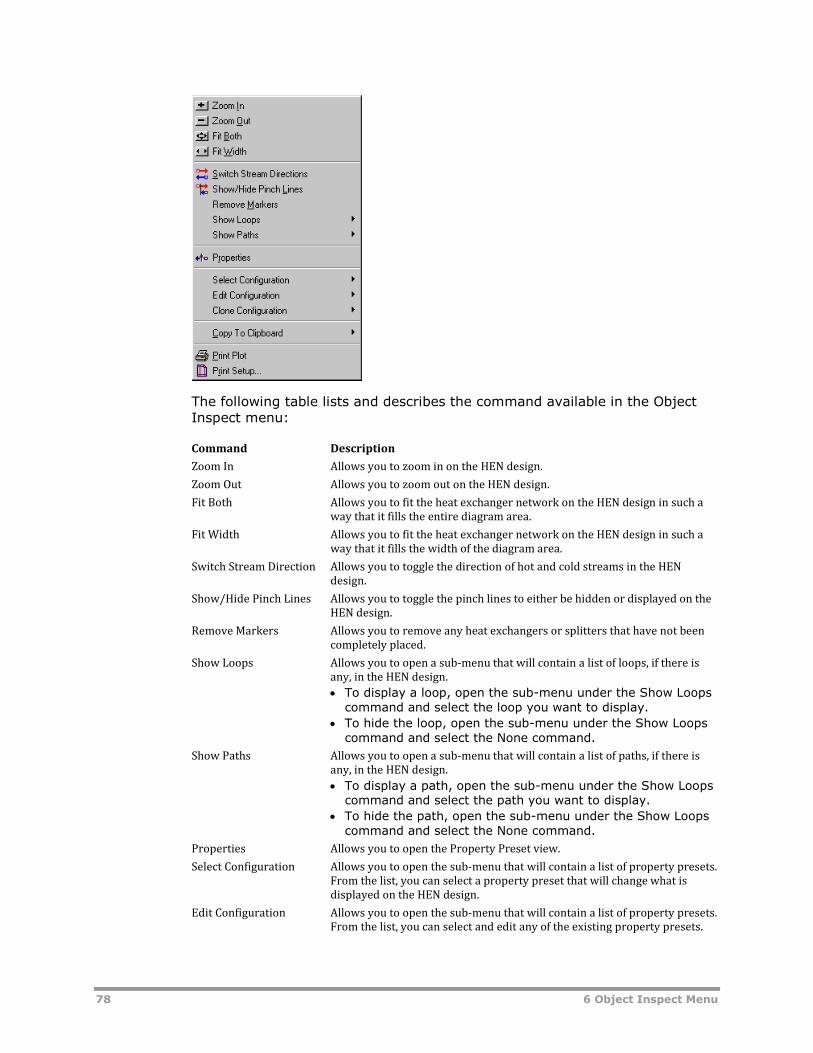
78 6 Object Inspect Menu
The following table lists and describes the command available in the ObjectInspect menu:
Command Description
Zoom In Allows you to zoom in on the HEN design.
Zoom Out Allows you to zoom out on the HEN design.
Fit Both Allows you to fit the heat exchanger network on the HEN design in such away that it fills the entire diagram area.
Fit Width Allows you to fit the heat exchanger network on the HEN design in such away that it fills the width of the diagram area.
Switch Stream Direction Allows you to toggle the direction of hot and cold streams in the HENdesign.
Show/Hide Pinch Lines Allows you to toggle the pinch lines to either be hidden or displayed on theHEN design.
Remove Markers Allows you to remove any heat exchangers or splitters that have not beencompletely placed.
Show Loops Allows you to open a sub-menu that will contain a list of loops, if there isany, in the HEN design.
• To display a loop, open the sub-menu under the Show Loopscommand and select the loop you want to display.
• To hide the loop, open the sub-menu under the Show Loopscommand and select the None command.
Show Paths Allows you to open a sub-menu that will contain a list of paths, if there isany, in the HEN design.
• To display a path, open the sub-menu under the Show Loopscommand and select the path you want to display.
• To hide the path, open the sub-menu under the Show Loopscommand and select the None command.
Properties Allows you to open the Property Preset view.
Select Configuration Allows you to open the sub-menu that will contain a list of property presets.From the list, you can select a property preset that will change what isdisplayed on the HEN design.
Edit Configuration Allows you to open the sub-menu that will contain a list of property presets.From the list, you can select and edit any of the existing property presets.
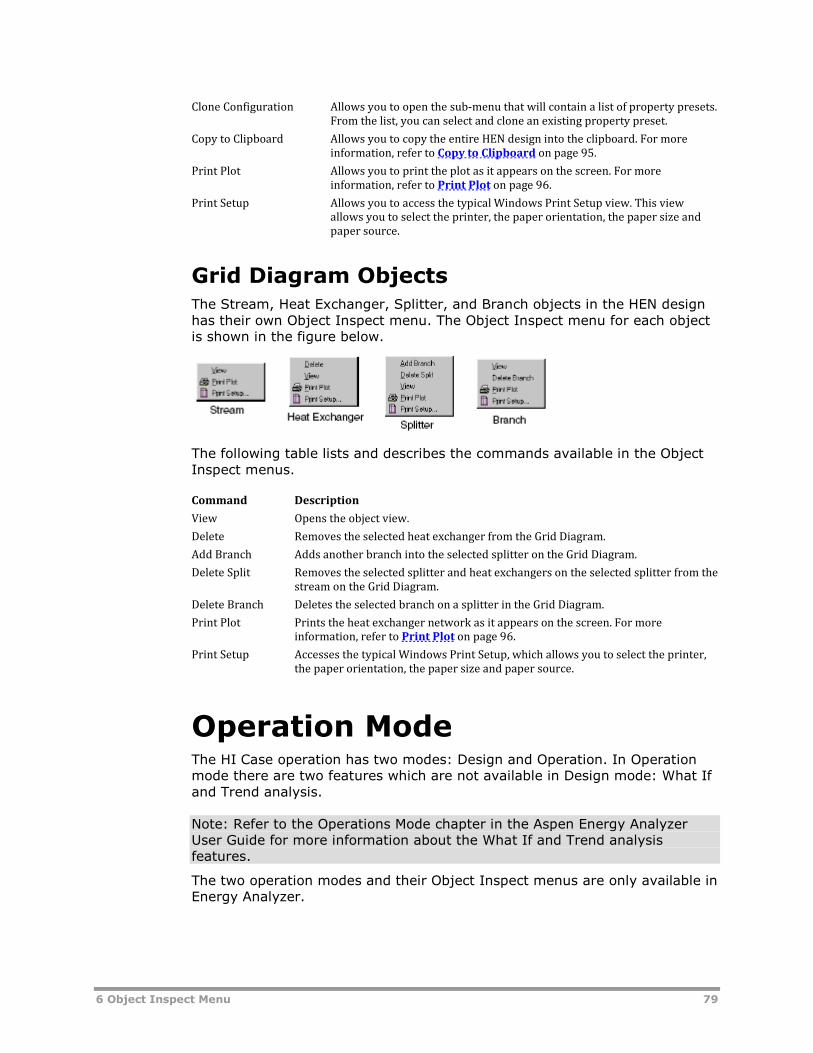
6 Object Inspect Menu 79
Clone Configuration Allows you to open the sub-menu that will contain a list of property presets.From the list, you can select and clone an existing property preset.
Copy to Clipboard Allows you to copy the entire HEN design into the clipboard. For moreinformation, refer to Copy to Clipboard on page 95.
Print Plot Allows you to print the plot as it appears on the screen. For moreinformation, refer to Print Plot on page 96.
Print Setup Allows you to access the typical Windows Print Setup view. This viewallows you to select the printer, the paper orientation, the paper size andpaper source.
Grid Diagram ObjectsThe Stream, Heat Exchanger, Splitter, and Branch objects in the HEN designhas their own Object Inspect menu. The Object Inspect menu for each objectis shown in the figure below.
The following table lists and describes the commands available in the ObjectInspect menus.
Command Description
View Opens the object view.
Delete Removes the selected heat exchanger from the Grid Diagram.
Add Branch Adds another branch into the selected splitter on the Grid Diagram.
Delete Split Removes the selected splitter and heat exchangers on the selected splitter from thestream on the Grid Diagram.
Delete Branch Deletes the selected branch on a splitter in the Grid Diagram.
Print Plot Prints the heat exchanger network as it appears on the screen. For moreinformation, refer to Print Plot on page 96.
Print Setup Accesses the typical Windows Print Setup, which allows you to select the printer,the paper orientation, the paper size and paper source.
Operation ModeThe HI Case operation has two modes: Design and Operation. In Operationmode there are two features which are not available in Design mode: What Ifand Trend analysis.
Note: Refer to the Operations Mode chapter in the Aspen Energy AnalyzerUser Guide for more information about the What If and Trend analysisfeatures.
The two operation modes and their Object Inspect menus are only available inEnergy Analyzer.

80 6 Object Inspect Menu
What If Analysis ViewThe What If feature allows you access to the What If Analysis view. This viewis similar to the project view, except the view only contains two panes:Viewer and Results.
The following table lists and describes the Object Inspect menus available inthe Viewer and/or Results pane:
Object Inspect menu Command Description
Right-click in any blank area ofthe Viewer or Results pane toaccess this menu.
PrintDatasheet
Lists the available Datasheets for the currentlyactive object. You can highlight a Datasheet andeither preview or print it. Refer to PrintingDatasheet on page 29 for more details.
This command is only available for the Viewerpane.
MaximizeFrame
Maximizes the selected pane so that it is the onlyone visible in the view.
When viewing a maximized pane, you can stillaccess the other two panes by clicking anddragging the double border now situated at thepane's edges.
OpenFrame
Opens a new view that displays only the selectedpane/tab.
ResetFrame
Restores the selected pane to default size.
Open Page Opens the selected/active tab in a separate view.
This command is only available for the Resultspane.
Select an event type and right-click in the list to access thismenu
AddSchedule
Allows you to add an event to the What If analysis.You can have more than one event in the What Ifanalysis.
Select an event and right-click inthe list to access this menu.
Add Task Allows you to add a task to the selected/activeevent. You can have more than one task in anevent.
DeleteEvent
Allows you to delete the selected event.
ExecuteEvent
Allows you to execute/perform the task(s) withinthe selected event.
RenameEvent
Allows you to rename the selected event.
Select a task and right-click in thelist to access this menu.
Delete Task Allows you to delete the selected task.
Trend Analysis ViewThe Trend feature allows you access to the Trend Analysis view. This view issimilar to the project view, except the view only contains two panes: Viewerand Results.

6 Object Inspect Menu 81
The following table lists and describes the Object Inspect menus available inthe Viewer and/or Results pane:
Object Inspect menu Command Description
Right-click in any blank area of theViewer or Results pane to access thismenu.
Print Datasheet Lists the available Datasheets for thecurrently active object. You canhighlight a Datasheet and eitherpreview or print it. Refer to PrintingDatasheet on page 29 for moredetails.
This command is only available forthe Viewer pane.
Maximize Frame Maximizes the selected pane so that itis the only one visible in the view.
When viewing a maximized pane, youcan still access the other two panes byclicking and dragging the doubleborder now situated at the pane'sedges.
Open Frame Opens a new view that displays onlythe selected pane/tab.
Reset Frame Restores the selected pane to defaultsize.
Select the summary level and right-click in the list to access this menu.
Add Study Allows you to add a study to theTrend analysis. You can have morethan one study in the Trend analysis.
Select a study and right-click in thelist to access this menu.
Change Throughput Allows you to change the flow rate ofall the streams simultaneously.
Clean Exchanger /Change Massflow
Allows you to add an event (cleaning aheat exchanger or change the massflow rate of a stream) to the selectedstudy. You can have more than oneevent in a study.
Delete Study Allows you to delete the selectedstudy.
Execute Study Allows you to execute/perform theevent(s) within the selected study.
Rename Study Allows you to rename the selectedstudy.
Select an event and right-click in thelist to access this menu.
Delete Event Allows you to delete the selectedevent.

82 6 Object Inspect Menu

7 Plot Properties 83
7 Plot Properties
IntroductionMany properties and results in this software can be viewed in graphical form.In order to customize your plot:
1 Right-click the plot area and the Object Inspect menu appears.
The Object Inspect menu shown in the figure below belongs to a two-axesplot. If a plot has three- or four-axes, than the commands in the ObjectInspect menu will vary.
2 Move the mouse pointer over the command you want to execute.
3 Click the highlighted command to select/execute the command you wantto use to manipulate the plot.
The following commands are common for most plots:
• Graph Control
• Values
• Copy to Clipboard
• Print Plot
• Print Setup
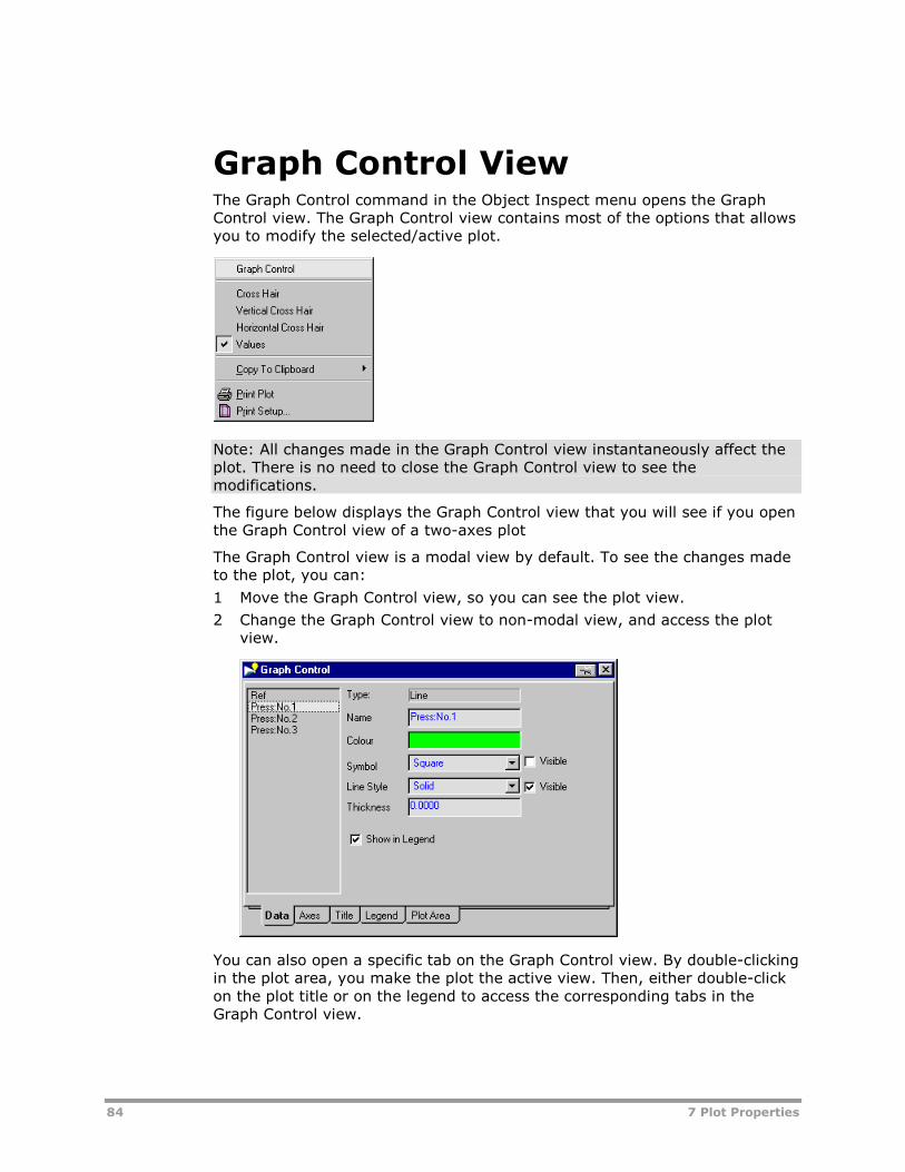
84 7 Plot Properties
Graph Control ViewThe Graph Control command in the Object Inspect menu opens the GraphControl view. The Graph Control view contains most of the options that allowsyou to modify the selected/active plot.
Note: All changes made in the Graph Control view instantaneously affect theplot. There is no need to close the Graph Control view to see themodifications.
The figure below displays the Graph Control view that you will see if you openthe Graph Control view of a two-axes plot
The Graph Control view is a modal view by default. To see the changes madeto the plot, you can:
1 Move the Graph Control view, so you can see the plot view.
2 Change the Graph Control view to non-modal view, and access the plotview.
You can also open a specific tab on the Graph Control view. By double-clickingin the plot area, you make the plot the active view. Then, either double-clickon the plot title or on the legend to access the corresponding tabs in theGraph Control view.

7 Plot Properties 85
While the plot area has focus, you can also click and drag on either the legendor title to reposition the selected item.
Note: The changes made to a plot using the Graph Control view are specific tothe active plot. To make global changes, which will affect all plots, use theColors and Fonts pages on the Resources tab of the Session Preferences view.
The options use to modify many of the plot characteristics, are categorizedinto the five tabs in the Graph Control view: Data, Axes, Title, Legend, andPlot Area
Data TabFor each data set on the plot, you can:
• View the data set Type.
• Modify the data set Name.
• Specify the Color and Symbol that represent the data on the plot.
• Choose a Line Style.
• Show/hide the Symbol or Line.
• Show/hide the name in the Legend.
Any changes that are made affect only the data set that is selected in the list.
To make modifications to the appearance of a data set:
1 Select the name of the data set from the list located at the left side of theData tab.
2 The information which corresponds to the selected data set appears in thefields, as shown below.
The figure on the right is the Graph Control view of a two-axes plot. Thefigure on the left is the Graph Control view of a three-axes plot.

86 7 Plot Properties
The following table lists and describes the objects in the Data tab view forboth type of plots:
Object Description
Type Display field The program has two types of plot: Line or Bar. This field shows you whichtype of plot the data set is using.
This field is only available for the two-axes plot.
Name field The name associated with the data set can be changed in this field. Changesmade to the text in this field are reflected in the list of data sets and in thelegend.
Color selector Allows you to change the color associated to the selected data set. To changethe color of the data set:
• Double-click in the selector to open the Color Palette, select acolor from the default color, and then click the OK button.
• Customize a color by clicking the Define Custom Colors buttonand generating your customized color. Then select your customcolor and click the OK button.
Symbol drop-downlist
For two-axes plot, the Symbol drop-down list allows you to select the type ofsymbol you want associated to your data set.
To display the symbols along the plot line of the data set, you have to check theVisible checkbox. To hide the symbols, uncheck the Visible checkbox.
Symbol group For three-axes plot, the Symbol group contains the following objects:
• Style drop-down list. This drop-down list has the same functionas the Symbol drop-down list from the two-axes plot.
• Scale field. This field allows you to modify the size of thesymbol. There are only three sizes available, and they arerepresented by integer values (1-3).
• Visible checkbox. This checkbox has the same function as theVisible checkbox from the two-axes plot.
Line Style drop-down list
For two-axes plot, this drop-down list allows you to select the type of plot lineyou want associated to your data set.
To display the plot line of the data set, you have to check the Visible checkbox.To hide the plot line, uncheck the Visible checkbox.
Thickness field For two-axes plot, this field sets the thickness of the plot line for the selecteddata set. Increasing the value in this field increases the thickness. You can onlyenter integer values (0-5).
Line group For three-axes plot, the Line group contains a Style drop-down list, a Thickfield, and a Visible checkbox.
• Style drop-down list. This drop-down list has the same functionas the Line Style drop-down list from the two-axes plot.
• Thick field. This field has the same function as the Thicknessfield from the two-axes plot.
• Visible checkbox. This checkbox has the same function as theVisible checkbox from the two-axes plot.
Show in Legendcheckbox
Allows you to toggle between displaying or hiding the data set name and plotline in the Legend.
Show Labelcheckbox
Allows you to toggle between displaying or hiding the data point value (boilingpoint temperature) on the plot/graph.
Axes TabFor each axis on the plot, you can:
• Change the label name, font, and units.

7 Plot Properties 87
• Show/Hide the label name and/or units.
• Define the axis bounds or use the Auto Scale function.
• Format the axis values.
• Display the plot on a logarithmic axis
Any changes that are made will affect only the axis that is selected in the list.Refer to Variables Tab on page 41 for information regarding valueformatting.
To make modifications to the appearance of an axis:
1 Select the name of the axes in the list located at the left side of the Axestab.
2 The information that corresponds to the selected axis appears in thefields, as shown below.
The figure on the right is the Graph Control view of a two-axes plot. Thefigure on the left is the Graph Control view of a three-axes plot.

88 7 Plot Properties
The following table lists and describes the objects in the Axes tab for bothplots:
Object Description
Label group fortwo-axes plot
This group contains the following objects:
• Label Field. This field allows you to change the label name for theselected axis.To display the label name beside the axis, check the Visiblecheckbox beside the Label field. To hide the label name, uncheckthe Visible checkbox.
• Label Drop-down list. This drop-down list contains all the possibleunits for the selected axis. You can select the units you want theselected axis to display.To display the unit type beside the axis, check the Visible checkboxbeside the Label drop-down list. To hide the unit type, uncheck theVisible checkbox.
• Label Font Selector. The font selector (located in the right side ofthe Label group) allows you to customize the font style and fontsize of the label. Double-click the font selector to open the Fontview.
Label group forthree-axes plot
This group contains the following objects:
• Side Field. This field has the same function as the Label field of thetwo-axes plot. The label appears along the axes.
• Vertex Field. This field allows you to modify the name associatedwith the selected axes. The name appears at the beginning of theaxes.To display the name at the beginning of the axis, check the Visiblecheckbox beside the Label field. To hide the label name, uncheckthe Visible checkbox.
Bounds group The Bounds group is only available for the two-axes plot. There are two fields andtheir associated checkbox in this group: Minimum and Maximum.
Minimum:
There are two ways to set the minimum axis bound value in the Bounds group:
• Uncheck the Use Auto Scale checkbox beside the Minimum field,and enter the minimum value you want in the Minimum field.
• Check the Use Auto Scale checkbox beside the Minimum field tohave the program automatically set the minimum bound value.
Maximum:
There are two ways to set the maximum axis bound value in the Bounds group:
• Uncheck the Use Auto Scale checkbox beside the Maximum field,and enter the maximum value you want in the Maximum field.
• Check the Use Auto Scale checkbox beside the Maximum field tohave the program automatically set the maximum bound value.
Logarithmic Axischeckbox
Check this checkbox to display the selected axis on a Logarithmic scale. Thischeckbox is only available for the two-axes plot.
Format field This display field allows you to modify the format of the selected axis values. Click
the Ellipsis icon beside the Format display field to open Real Format Editorview.
Title TabFor the title on the plot, you can:
• Change the default title name and font.
• Select the colors for the Text, Background, and Border of the title.

7 Plot Properties 89
• Show/Hide the Title, Background, and Border.
The figure on the right is the Graph Control view of a two-axes plot. Thefigure on the left is the Graph Control view of a three-axes plot.
The following table lists and describes the objects on the Title tab for bothplots:
Object Description
Text group The Text group contains the following objects:
• Text field. This field allows you to change the title of the plot.
• Visible checkbox. Check this checkbox to display the title on theplot. Uncheck this checkbox to hide the title.
• Color selector. This color selector allows you to change the titlefont color.
Font selector Allows you to customize the two-axes plot font style and font size of the title.Double-click the font selector to open the Font view.
Background group The Background group contains the following objects:
• Background color selector. This color selector allows you tochange the title background color.
• Visible checkbox. Check this checkbox to display the selectedbackground color for the title on the plot. Uncheck this checkboxto hide the background color.
Border group The Border group contains the following objects:
• Border color selector. This color selector allows you to change thetitle border color.
• Visible checkbox. Check this checkbox to display the borderaround the title on the plot. Uncheck this checkbox to hide theborder.

90 7 Plot Properties
To change the color of the title text, title background, or title border:
1 Double-click in the color selector, of the axes object you want to change,to open the Color Palette.
2 Select a color from the default color and click the OK button
or
3 Customize a color by clicking the Define Custom Colors button, select andadd you customized colors to the Custom colors palette. Then select yourcustom color and click the OK button.
Legend TabFor the legend on the plot, you can:
• Change the color of the border, background, or text.
• Change the location of the legend on the plot area.
• Choose the orientation: vertical or horizontal.
• Show/Hide the border and background.
• Enable automatic resizing of the legend upon repositioning.
The figure on the right is the Graph Control view of a two-axes plot. Thefigure on the left is the Graph Control view of a three-axes plot.

7 Plot Properties 91
The following table lists and describes the objects on the Legend tab:
Object Description
Visible checkbox Check the Visible checkbox to display the legend on the plot. Uncheck thischeckbox to hide the legend.
Border group The Border group contains the following objects:
• Border color selector. This color selector allows you to change thelegend border color.
• Visible checkbox. Check this checkbox to display the borderaround the legend on the plot. Uncheck this checkbox to hide theborder.
Background group The Background group contains the following objects:
• Background color selector. This color selector allows you tochange the legend background color.
• Visible checkbox. Check this checkbox to display the selectedbackground color for the legend on the plot. Uncheck thischeckbox to hide the background color.
Text group The Text group contains the Text color selector. This color selector allows you tochange the legend font color.
Font selector Allows you to customize the two-axes plot font style and font size in the legend.Double-click the font selector to open the Font view.
Alignment group The Alignment group contains the following objects:
• Dynamic checkbox. Check this checkbox to have the programresize the legend when it is repositioned in the plot area.For example, if the legend is placed near the view side wherepart of the information is cut off/hidden, the programautomatically resizes the legend to display the cut off/hiddeninformation.
• Vertical and Horizontal radio buttons. The two radio button allowsyou to set the orientation of the text in the legend. Select a radiobutton to position the legend information in a row or a column.
To change the color of the legend text, legend background, or legend border:
• Double-click in the color selector, of the axes object you want to change,to open the Color Palette, select a color from the default color, and thenclick the OK button
or
• Customize a color by clicking the Define Custom Colors button, select andadd you customized colors to the Custom Colors palette. Then select yourcustom color and click the OK button.

92 7 Plot Properties
Plot Area TabFor the area/background of the plot, you can:
• Change the color of the Background, Frame, or Grid.
• Show/Hide the Background, Frame, or Grid.
• Change the color of the Cross Hairs
• Show/Hide the Cross Hairs, or choose to display only the vertical orhorizontal components.
The figure on the right is the Graph Control view of a two-axes plot. Thefigure on the left is the Graph Control view of a three-axes plot.
The following table lists and describes the objects on the Plot Area tab forboth plots:
Object Description
Backgroundgroup
The Background group contains the following objects:
• Background color selector. This color selector allows you to changethe plot background color.
• Visible checkbox. Check this checkbox to display the selectedbackground color on the plot. Uncheck this checkbox to hide thebackground color.
Grid group The Grid group contains the following objects:
• Grid color selector. This color selector allows you to change the gridcolor in the plot.
• Visible checkbox. Check this checkbox to display the grid in the plot.Uncheck this checkbox to hide the grid.
Frame group The Frame group is only available for the two-axes plot. This group contains thefollowing objects:
• Frame color selector. This color selector allows you to change theframe color of the plot.
• Visible checkbox. Check this checkbox to display the frame aroundon the plot. Uncheck this checkbox to hide the frame.
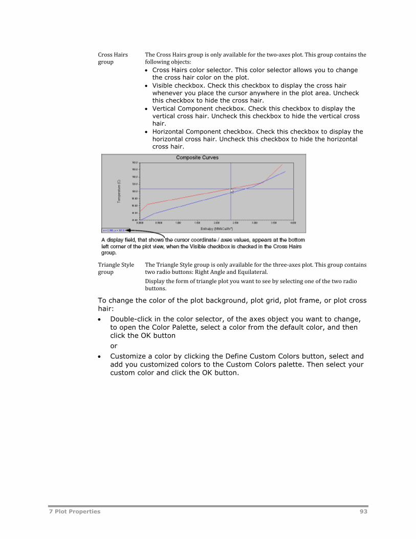
7 Plot Properties 93
Cross Hairsgroup
The Cross Hairs group is only available for the two-axes plot. This group contains thefollowing objects:
• Cross Hairs color selector. This color selector allows you to changethe cross hair color on the plot.
• Visible checkbox. Check this checkbox to display the cross hairwhenever you place the cursor anywhere in the plot area. Uncheckthis checkbox to hide the cross hair.
• Vertical Component checkbox. Check this checkbox to display thevertical cross hair. Uncheck this checkbox to hide the vertical crosshair.
• Horizontal Component checkbox. Check this checkbox to display thehorizontal cross hair. Uncheck this checkbox to hide the horizontalcross hair.
Triangle Stylegroup
The Triangle Style group is only available for the three-axes plot. This group containstwo radio buttons: Right Angle and Equilateral.
Display the form of triangle plot you want to see by selecting one of the two radiobuttons.
To change the color of the plot background, plot grid, plot frame, or plot crosshair:
• Double-click in the color selector, of the axes object you want to change,to open the Color Palette, select a color from the default color, and thenclick the OK button
or
• Customize a color by clicking the Define Custom Colors button, select andadd you customized colors to the Custom Colors palette. Then select yourcustom color and click the OK button.

94 7 Plot Properties
ValuesYou can toggle the Values command from the Object Inspect menu on or off.A checkmark appears on the left side of the Values command in the ObjectInspect menu, when the command is on. The left side of the Values commandin the Object Inspect menu is blank, when the command is off. See figurebelow:
When the Values command is on, you can place the cursor on a plotted pointin the plot area and a fly by of values (or coordinates) will appear.

7 Plot Properties 95
Copy to ClipboardCopy the area, plot, or PFD where the Object Inspect menu was accessed,and placed that image into the clipboard. The image can be taken and pastedinto other programs as an image file, like a word processor.
The Copy to Clipboard command opens a sub-menu that contains four scalecommands, shown in the figure below.
The scale commands let you decide how large an image you want to copy intothe clipboard. The four scale commands are: 50%, 100%, 200%, and customscale.
To copy a customize scale of the view/area:
1 Right-click in the area to access the Object Inspect menu.
2 Select Copy To Clipboard command to open the sub-menu.
3 In the Copy To Clipboard sub-menu, select Custom Scale command. TheCopy Pane to Clipboard view appears.
4 Enter the scale you want in the Copy at scale field.
5 Click the OK button when you are finish, or click the Close icon to exitwithout copying anything to the clipboard.

96 7 Plot Properties
Print PlotThere are two methods to print the plots in the program:
• Right-click the plot area to open the Object Inspect menu. Select the PrintPlot command from the Object Inspect menu as shown in the figurebelow. This method prints only the plot as it appears on the screen.
or
• Select the plot view you want to print, then click the File menu and selectthe Print Snapshot command. This method prints the plot along witheverything else in the view that has focus. For more information aboutprinting in general, refer to Print Commands on page 28.
Print SetupThe Print Setup option accesses the typical Windows Print Setup, which allowsyou to select the printer, the paper orientation, the paper size, and the papersource. There are two methods to open the Print Setup view:
• Right-click the plot area to open the Object Inspect menu. Select the PrintSetup command from the Object Inspect menu.
or
• Click the File menu and select Print Setup.
The Print Setup view will vary for different printers.

7 Plot Properties 97
Plot Orientation ViewThe Plot Orientation command from the Object Inspect menu opens the PlotOrientation view.
The following table lists and describes the icons in the Plot Orientation view:
Icons Description
Allows you to rotate the positions of the variables of the plot by one stepcounter clockwise.
Allows you to switch the position of the two variables between the icon.
Allows you to rotate the positions of the variables of the plot by one stepclockwise.

98 7 Plot Properties
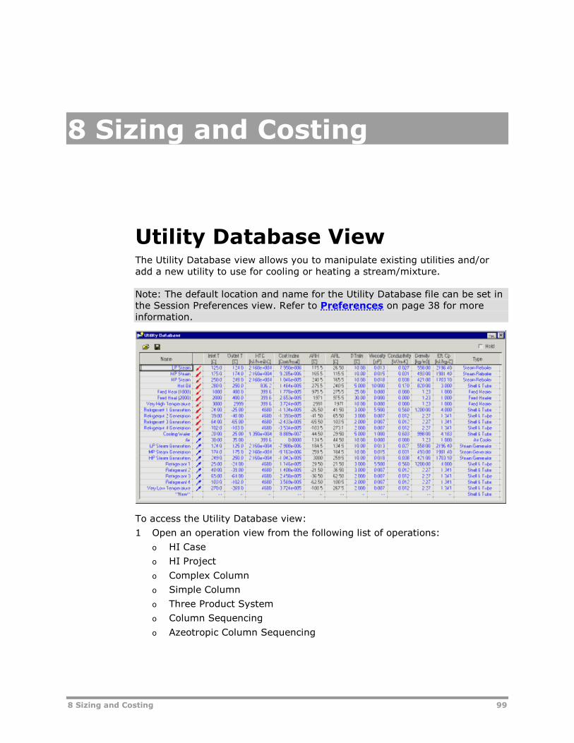
8 Sizing and Costing 99
8 Sizing and Costing
Utility Database ViewThe Utility Database view allows you to manipulate existing utilities and/oradd a new utility to use for cooling or heating a stream/mixture.
Note: The default location and name for the Utility Database file can be set inthe Session Preferences view. Refer to Preferences on page 38 for moreinformation.
To access the Utility Database view:
1 Open an operation view from the following list of operations:
o HI Case
o HI Project
o Complex Column
o Simple Column
o Three Product System
o Column Sequencing
o Azeotropic Column Sequencing
100 8 Sizing and Costing
Note: When accessing the Utility Database view from the HI Case or HIProject operation, you will see an extra button called Select Utility besidethe Save Default Utilities to File icon
2 Click the Options tab or page.
3 Click the Utility Database button.The Utility Database view will appear.
The following table lists and describes the objects available on the UtilityDatabase view:
Object Icon Description
Open Saved DefaultUtilities File icon
Allows you to open a utility database file. The file can be theprogram's default database file or a user defined utility databasefile.
Save Default Utilities toFile icon
Allows you to save the current settings in the Utility Databaseview as a file.
Select Utility button Allows you to add the selected utility to the heat exchangernetwork.
The Select Utility button is only available when accessing theUtility Database view from the HI Case or HI Project operation.
Name column Allows you to specify or edit the name of the utility.
Heating or Cooling icon Displays an icon to indicate whether the utility is used forheating or cooling.
HOT. A hot utility stream is cooled down in the heat exchangenetwork. The inlet temperature of a hot process stream is higherthan the outlet temperature.
COLD. A cold utility stream is heated up in the heat exchangenetwork. The inlet temperature of a cold process stream is lowerthan the outlet temperature.
Inlet T column Allows you to manipulate the temperature of the utility enteringthe heat exchanger.
Outlet T column Allows you to manipulate the temperature of the utility exitingthe heat exchanger.
HTC column Allows you to manipulate the heat transfer coefficient of theutility.
Cost Index column Allows you to manipulate the cost per energy/duty of the utility.
ARH column Displays the calculated Application Range High temperaturevalue.
ARL column Displays the calculated Application Range Low temperaturevalue.
DTmin column Allows you to specify or manipulate the minimum temperaturedifference of the utility.
Hold checkbox Allows you to toggle between calculating or not calculating theoperating cost.
When the Hold checkbox is checked, the program will hold onto/hide the information in the Utility Database view duringcalculation. When the checkbox is unchecked, the program willcalculate the operating cost using the current information in theUtility Database view.

8 Sizing and Costing 101
Adding a New UtilityTo add a new utility type to the database:
1 Open the Utility Database view by clicking the Utility Database button.
2 Click on the cell containing **New** in the Name column.
3 Enter the name of the new utility.
4 Click in the Inlet T cell and enter the temperature of the utility going intothe heat exchanger.
5 Click in the Outlet T cell and enter the temperature of the utility exitingthe heat exchanger.An icon to indicating whether the utility is used for heating or cooling willappear in the icon cell automatically.
6 Click in the HTC cell and enter the value for the heat transfer coefficient ofthe utility.
7 Click in the Cost Index cell and enter the value for the cost/duty of theutility.
8 Click in the DTmin cell and enter the value for the minimum temperaturedifference of the utility.
Deleting a UtilityTo delete a utility:
1 Ensure the current operation is not using the utility you want to delete.
2 Open the Utility Database view by clicking the Utility Database button.
3 In the Name column, click on the name of the utility you want to delete.
4 Press delete.
Note: The program will not prompt you to confirm deletion of a utility, so bevery careful when deleting a utility.
Saving the Utility DatabaseThe program allows you to save a utility database as a (*.hud) file.
To save the current utility database:
1 Open the Utility Database view by clicking the Utility Database button.
2 Modify the utility information to suit your simulation case.
3 Click the Save Default Utilities to File icon .
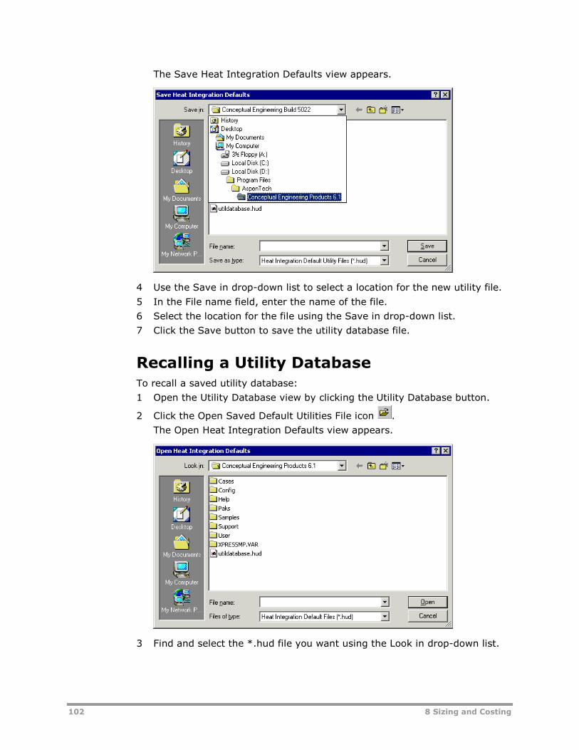
102 8 Sizing and Costing
The Save Heat Integration Defaults view appears.
4 Use the Save in drop-down list to select a location for the new utility file.
5 In the File name field, enter the name of the file.
6 Select the location for the file using the Save in drop-down list.
7 Click the Save button to save the utility database file.
Recalling a Utility DatabaseTo recall a saved utility database:
1 Open the Utility Database view by clicking the Utility Database button.
2 Click the Open Saved Default Utilities File icon .
The Open Heat Integration Defaults view appears.
3 Find and select the *.hud file you want using the Look in drop-down list.

8 Sizing and Costing 103
4 Click the Open button.The Utility Database view reappears displaying the selected utilitydatabase information.

104 8 Sizing and Costing
9 References 105
9 References
Agrawal, R. & Fidkowski, Z., "Simplified Thermally Coupled Arrangements for Ternary distillation", paper 221c inAnnual AIChE conference, Dallas, TX, 1999.
Agrawal, R. & Fidkowski, Z., "Preliminary Screening of Column Configurations for Ternary Distillation", Paper 1dpresented at Spring AIChE Meeting, New Orleans, LA, March 11-15, 2002.
Ahmad, S. & Linnhoff, B., Overall Cost Targets for Heat Exchanger Networks, IChemE Annual Research Meeting,Bath, UK, 1984.
Ahmad, S. & Linnhoff, B., Supertargetting: Different Process Structures for Different Economics, ASME J. EnergyResources Technology, 3, 131-136, 1989.
Ahmad, S. & Smith, R., Targets and Design for Minimum Number of Shells in Heat Exchanger Networks, Chem.Engng. Res. Dev., 67, 481-494, 1989.
Ahmad, S., Linnhoff, B., & Smith, R., Cost Optimal Heat Exchanger Networks-2. Targets and Design for DetailedCapital Cost Models, Comp. Chem. Engng., 14(7), 751-767, 1990.
Andersen, H.W., Laroche, Lionel, & Morari, Manfred, Effect of design on the operation of homogenous azeotropicdistillation. CCE 19, 105, 1994.
Anderson, Nancy J. & Doherty, Michael F., An approximate model for binary azeotropic distillation design. CES39(1), 11-19, 1984.
Anderson, T.F., Abrams, D.J. & E.A. Green II, Evaluation of Parameters for Nonlinear Thermodynamic Models,AIChE J. Vol 24; No. 1, 1978.
Apelblat, Alexander & Wisniak, Jaime, A simple method for evaluating the Wilson constant. IECR 28, 324, 1989.
Asante, N.D.K. & Zhu, X.X., An Automated and Interactive Approach for Heat Exchanger Network Retrofit, TransIChemE, 75(A), 349-360, 1997.
Bauer, M.H. & Stichlmair, Johann, Synthesis and optimization of distillation sequences for the separation ofazeotropic mixtures. CCE 19 Supl., S15, 1995.
Bausa, J., Watzdorf, R.V., Marquardt, W., "Shortcut Methods for Nonideal Multicomponent Distillation: 1. SimpleColumns", AIChE J., 44 (10), 1998.
Bekiaris, Nikolaos, Meski, George A., Radu, Cristian M., & Morari, Manfred, Multiple steady states in homogeneousazeotropic distillation. IECR 32, 2023, 1993.
Bekiaris, Nikolaos, Meski, George A., Radu, Cristian M., & Morari, Manfred, Design and control of homogeneousazeotropic distillation columns. CCE 18 Suppl., S15, 1994.
Benedict, Manson & Rubin, Louis C., Extractive and azeotropic distillation. I. Theoretical aspects. TAICHE 41, 353,1945.
Benedict, Manson, Johnson, C.A., Solomon, Ernest, & Rubin, Louis C., Extractive and azeotropic distillation. II.Separation of toluene from paraffins by azeotropic distillation with methanol. TAICHE 41, 371, 1945.
Biegler, L.T., Grossmann, I.E., & Westerberg, A.W., Systematic Methods of Chemical Process Design, Prantice Hall,New Jersey, USA, 1997.
Boland, D. & Linnhoff, B., The Preliminary Design of Networks for Heat Exchange by Systematic Methods, The.Chem. Engr., April, 9-15, 1979.
Bossen, Bjarne S., Jorgensen, Sten Bay, & Gani, Rafiqul, Simulation, design and analysis of azeotropic distillationoperations. IECR 32, 620, 1993.
Briones, V. & Kokossis, A., Targeted Transhipment Model for Heat Exchanger Network Synthesis, Paper presentedat IChemE Annl. Res. Mtg., 1995.
Cerda, J., Westerburg, A.W., Mason, D., & Linnhoff, B., Minimum Utility Usage in Heat Exchanger NetworkSynthesis. A Transportation Problem, Chem. Eng. Sci., 38(3), 373-387, 1983.

106 9 References
Cerda, J. & Westerburg, A.W., Synthesizing Heat Exchanger Networks having Restricted Stream/Stream Matchesusing Transportation problem Formulations, Chem. Eng. Sci., 38(10), 1723-1740, 1983.
Cerda, J., Galli, M.R., Camussi, N., & Isla, M. A., Synthesis of Flexible Heat Exchanger Networks-I. ConvexNetworks, Comp. Chem. Engng., 14, 197, 1990.
Chemical Engineering, Vol. 17, No. 12, p. 1141-1155, 1993.
Ciric, A.R. & Floudas, C.A., Heat Exchanger Network Synthesis without Decomposition, Comp. Chem. Engng.,15(6), 385-396, 1991.
Colberg, R.D. & Morari, M., Area and Capital Cost Targets for Heat Exchanger Network Synthesis with ConstrainedMatches and Unequal Heat Transfer Coefficients, Comp. Chem. Engng., 14(1), 1-22, 1990.
Corripio, A.B., Chrien, K.S., Evans, L.B., "Estimate Costs of Heat Exchangers and Storage Tanks via Correlations,"Chem. Eng., January 25, 125-127, 1982.
Daichendt, M.M. & Grossmann, I.E., Preliminary Screening procedure for the MINLP Synthesis of Process Systems -II. Heat Exchanger Networks, Comp. Chem. Engng., 18(8), 679-709, 1994.
Diwekar, Urmila, An efficient design method for binary, azeotropic batch distillation columns. AICHE 37, 1571,1991.
Doherty, Michael F. & Perkins, J.D., Properties of liquid-vapour composition surfaces at azeotropic points. CES 32,1112, 1977.
Doherty, Michael F. & Perkins, J.D., On the Dynamics of Distillation Processes, CES 33, 281-301, 1978.
Doherty, Michael F., The presynthesis problem for homogeneous azeotropic distillation has a unique explicitsolution. CES 40, 1885, 1985.
Doherty, Michael F. & Caldarola, Glenn A., Design and synthesis of homogeneous azeotropic distillation. 3. Thesequencing of columns for azeotropic and extractive distillations. IECF 24, 474, 1985.
Doherty, Michael F. & Malone, M.F., Short Course on Distillation Design, Course Notes.
Doherty, M.F. & Malone, M.F., Conceptual Design of Distillation systems, McGraw-Hill, New York, 2001.
Douglas, J.M., Conceptual Design of Chemical Processes, McGraw Hill Book Company, New York, USA, 1988.
Duran, M.A. & Grossmann, I.E., Simultaneous Optimization and Heat Integration of Chemical Processes, AIChE J.,32(1), 123-138, 1986.
Dussel, Ralf & Stichlmair, Johann, Separation of azeotropic mixtures by batch distillation using entrainers. CCE 19Supl., S113, 1995.
Edgar, T.F. & Himmelblau, D.M., Optimization of Chemical Processes, McGraw Hill, Inc. 1986.
Fidkowski, Z. & Krolikowski, L., "Thermally Coupled System of Distillation Columns: Optimisation Procedure," AIChEJ., 32, 537-546, 1986.
Fidkowski, Z. & Krolikowski, L., "Minimum Energy Requirements of Thermally Coupled Distillation Systems," AIChEJ., 33, 643-653, 1987.
Fidkowski, Z.T., Malone, M.F., & Doherty, Michael F., Nonideal multicomponent distillation: Use of bifurcationtheory for design. AICHE 37, 1761-1779, 1991.
Fidkowski, Z.T., Malone, Michael F., & Doherty, Michael F., Computing azeotropes in multicomponent mixtures. CCE17, 1141, 1993a.
Fidkowski, Z.T., Doherty, Michael F., & Malone, Michael F. Feasibility of separations for distillation of nonidealternary mixtures. AICHE 39, 1303, 1993b.
Fien, Gert-Jan A.F. & Liu, Y.A., Heuristic synthesis and shortcut design of separation processes using residue curvemaps: a review. IECR 33, 2505, 1994.
Fisher, Wayne R., Doherty, Michael F., Douglas, James M., Shortcut calculation of optimal recovery fractions fordistillation columns. iecpdd 24, 955, 1985.
Floudas, C.A., Ciric A.R., & Grossmann, I.E., Automatic Synthesis of Optimal Heat Exchanger Network Synthesis,AIChE Journal, 32(2), 276-290, 1986.
Floudas, C.A. & Ciric A.R., Strategies for Overcoming Uncertainties in Heat Exchanger Network Synthesis, Comp.Chem. Engng., 13(10), 1133-1152, 1989.
Floudas, C.A., Nonlinear and Mixed-Integer Optimization: Fundamentals and Applications, Oxford University Press,Oxford, 1995.
Flower, J. A. & Linnhoff B., A Thermodynamic-Combinatorial Approach to the Design of Optimum Heat ExchangerNetworks, AIChE J., 26(1), 1-9, 1980.

9 References 107
Foucher, Etienne R., Doherty, Michael F., Malone, Michael F., Automatic screening of entrainers for homogeneousazeotropic distillation. IECR 30, 760, 1991.
Glanz, S. & Stichlmair, Johann, Energetic optimization of distillations in hybrids processes. CCE 19 Supl., S51,1995.
Gmehling, J. & Onken, U., Vapor-Liquid Equilibrium Data Collection - Aqueous-Organic Systems, DECHEMAChemistry Data Series Vol.I, Part 1, 1977.
Gundersen, T., Duvold, S., & Ahmady, A. H., An Extended Vertical MILP Model for Heat Exchanger NetworkSynthesis, Comp. Chem. Engng., 20, S97-S102, 1996.
Gundersen, T., Traedal, P., & Ahmady, A. H., Improved Sequential strategy for the Synthesis of Near-Optimal HeatExchanger Networks, Comp. Chem. Engng., 21, S59-S64, 1997.
Gundersen, T. & Naess, L., The Synthesis of Cost Optimal Heat Exchanger Networks: An Industrial Review of theState of the Art, Comp. Chem. Engng., 12(6), 503-530, 1988.
Gundersen, T. & Grossmann, I.E., Improved Optimisation Strategies for Automated Heat Exchanger NetworksSynthesis through Physical Insights, Comp. Chem. Engng., 14(9), 925-944, 1990.
Guttinger, Thomas E., Dorn, Cornelius, & Morari, Manfred, Experimental study of multiple steady states inhomogeneous azeotropic distillation. IECR 36(3), 794-802, 1997.
Hall, S.G., Ahmad, S., & Smith, R., Capital Cost Targets for Heat Exchanger Network Comprising Mixed Materials ofConstruction, Pressure Ratings and Exchanger Types, Comp. Chem. Engng., 14(3), 319-335, 1990.
Hohmann, E. C., Optimal Networks for Heat Exchanger, Ph. D. Thesis, University of Southern California, USA,1971.
Holland, C.D., Gallun, S.E., Lockett, M.J., Modeling azeotropic and extractive distillations. CE Mar 23, 185, 1981.
Hunek, J., Gal, S., Posel, F., Glavic, P., Separation of an azeotropic mixture by reverse extractive distillation. AICHE35, 1207, 1989.
Jezowski, J., A Simple Synthesis Method for Heat Exchanger Networks with Minimum Number of Matches, Comp.Chem. Engng., 45(7), 1928-1932, 1990.
Jezowski, J., The Pinch Design Method for Tasks with Multiple Pinches, Comp. Chem. Engng., 16(2), 129-133,1992a.
Jezowski, J., SYNHEN - Microcomputer Directed Package of Programs for Heat Exchanger Network Synthesis,Comp. Chem. Engng., 16(7), 691-706, 1992b.
Julka,Vivek & Doherty, Michael F., Geometric nonlinear analysis of multicomponent nonideal distillation: A simplecomputer-aided design procedure, Chem. Eng. Sci., 48(8), 1367-1391, 1993.
Kemp, I. C., Some Aspects of The Practical Application of Pinch Technology Methods, Trans IChemE Part A, 75,471, 1991.
Kienle, A., Gilles, E.D., Marquardt, W., Computing multiple steady states in homogeneous azeotropic distillationprocesses. CCE 18 Suppl., S37, 1994.
King, C.J., Separation Processes, 2 nd Ed., McGraw Hill Inc, 1980.
Kister, H.Z. Distillation Design, McGraw Hill Inc 1992.
Knapp, Jeffrey P. & Doherty, Michael F., Thermal integration of homogeneous azeotropic distillation sequences.AICHE 36, 969, 1990.
Knapp, Jeffrey P. & Doherty, Michael F., A new pressure-swing-distillation process for separating homogeneousazeotropic mixtures. IECR 31, 346, 1992.
Knapp, Jeffrey P. & Doherty, Michael F., Minimum entrainer flows for extractive distillation: A bifurcation theoreticapproach. AICHE 40, 243, 1994.
Knight, Jennifer R. & Doherty, Michael F., Design and synthesis of homogeneous azeotropic distillation. 5. Columnswith nonnegligible heat effects. IECF 25, 279, 1986.
Knight, Jennifer R. & Doherty, Michael F., Optimal design and synthesis of homogeneous azeotropic distillationsequences. IECR 28, 564, 1989.
Koehler, J.W., Aguirre, P., Blass, E., Minimum reflux calculations for nonideal mixtures using the reversibledistillation model. CES 46, 3021, 1991.
Kondratev, A.A., Serafinov, L.A., Akhmadeev, M.G., Calculation of azeotropic and extractive rectification on anelectronic computer. TFCE 13, 125, 1979.
Kotjabasakis, E. & Linnhoff, B., Sensitivity Tables for the Design of Flexible processes (1) - How Much Contingencyin Heat Exchanger Networks is Cost-Effective, Chem. Eng. Res. Dev, May, 64, 197-211, 1986.
108 9 References
Kurum, S. & Fonyo, Z., Comparative study of recovering acetic acid with energy integrated schemes. ATE 16(6),487, 1996.
Laroche, Lionel., Bekiaris, Nikolaos., Andersen, Henrik W., Morari, Manfred., The curious behaviour ofhomogeneous azeotropic distillation - implications for entrainer selection. AICHE 38, 1309, 1992.
Laroche, Lionel., Bekiaris, Nikolaos., Andersen, Henrik W., Morari, Manfred., Homogeneous azeotropic distillation:Separability and flowsheet synthesis. IECR 31, 2190, 1992.
Laroche, Lionel., Bekiaris, Nikolaos., Andersen, Henrik W., Morari, Manfred., Homogeneous azeotropic distillation:Comparing entrainers. CJCE 69, 1302, 1991.
Lestak, F., Smith, R., Dhole, V.R., "Heat Transfer across the wall of the Dividing Wall Columns" Trans IChemE, 72A,639-644, 1994.
Levy, Sanford G. & Doherty, Michael F., Design and synthesis of homogeneous azeotropic distillation. 4. Minimumreflux calculations for multiple-feed columns. IECF 25, 269, 1986.
Levy, Sanford G., Van Dongen, David B., Doherty, Michael F., Design and synthesis of homogeneous azeotropicdistillation. 2. Minimum reflux calculations for nonideal and azeotropic columns. IECF 24, 463., 1985.
Linnhoff, B. & Flower, J. A., Synthesis of Heat Exchanger Networks - I. Systematic Generation of Energy OptimalNetworks, AIChE Journal, 24(4), 633-642, 1978a.
Linnhoff, B. & Flower, J. A., Synthesis of Heat Exchanger Networks - II. Evolutionary Generation of Networks withVarious Criteria of Optimality, AIChE Journal, 24(4), 642-654, 1978b.
Linnhoff, B., Townsend, D.W., Boland, D., Hewitt, G.F., Thomas, B.E.A., Guy, A.R., Marsland, R.H., A User Guideon Process Integration for the Efficient use of Energy, IChemE England, 1982.
Linnhoff, B., New Concepts in Thermodynamics for Better Chemical Process Design, Chem. Eng. Res. Des., 61,July, 207-223, 1983.
Linnhoff, B. & Hindmarsh E., The Pinch Design Method for Heat Exchanger Networks, Chem. Eng. Sci., 38(5), 745-763, 1983.
Linnhoff, B., "The Process/Utility Interface", Second International Meeting, "Rational Use of Energy", Liege,Belguim, 1986.
Linnhoff, B., Kotjabasakis, E., & Smith, R., Flexible Heat Exchanger Network Design: Problem Definition and OneMethod of Approach, Paper 79d, AIChE Annual meeting, Washington DC, Nov 27-Dec 2, USA, 1988.
Linnhoff, B., Pinch Technology for the Synthesis of Optimal Heat and Power Systems, Transactions of ASME,Journal of Energy Resources Technology, 111(3), 137-147, 1989.
Linnhoff, B. & Ahmad, S., Supertargeting: Optimum Synthesis of Energy Management Systems, ASME J. EnergyResources Tech., 111, 121-130, 1989.
Linnhoff, B. & Ahmad, S., Cost Optimal Heat Exchanger Networks-I. Minimum Energy and Capital using SimpleModels for Capital Cost, Comp. Chem Engng., 14(7), 729-750, 1990.
Linnhoff, B., "Pinch Analysis: A State-of-the-Art Overview," Trans IChemE, Part A, 71, 503-522, 1993.
Matsuyama, Hisayoshi, Restrictions on patterns of residue curves around heterogeneous azeotropes. JCEJ 11, 427,1978.
Mekiffer, Olaf & Hartmann, Klaus, Definition and computation of distillation boundaries - A new approach.ICHEMESS 128, A91, 1992.
Michelsen, M.L., "The isothermal flash problem. I. Stability Analysis." Fluid Phase Equilibria., 9, p. 1, 1982.
Mulet, A., Corripio, A.B., Evans, L.B., "Estimate Costs of Pressure Vessels via Correlations", Chem. Eng., October 5,145-150, 1981a.
Mulet, A., Corripio, A.B., Evans, L.B., "Estimate Costs of Distillation and Absorption Towers via Correlations",Chem. Eng., December 28, 77-82, 1981b.
Nishida, N., Stephanopoulos, G., & Westerberg, A. W., A Review of Process Synthesis, AIChE Journal, 27, 321-351,1981.
O'Young, L. & Linnhoff, B., Degree of Freedom Analysis and a Systematic Procedure for the Design and Evolution ofConstrained Heat Exchanger Networks, AIChE Spring Meeitng, April, Houston, 1989.
Papalexandri, K.P. & Pistikopoulos, E.N., Synthesis of Cost Optimal and Controllable Heat Exchanger Networks,Trans. IChemE. Chem. Eng. Res. Dev., Part A, 350-356, 1994.
Papoulias, S.A. & Grossmann, I.E., A Structural Optimisation Approach in Process Synthesis - II Heat RecoveryNetworks, Comp. Chem. Engng, 7(6), 707-721, 1983.
9 References 109
Parker, S. J., Supertargeting for multiple utilities, Ph.d. Thesis, University of Manchester Institute of Science andTechnology, Manchester, UK, 1989.
Perry, R.H. & D.W. Green. Perry's Chemical Engineers' Handbook (Seventh Edition), McGraw-Hill, 1997.
Petlyuk, F.B., Thermodynamically reversible fractionantion process of multicomponent azeotropic mixtures. TFCE,270, 1978.
Petlyuk, F.B., Structure of concentration space and synthesis of schemes for separating azeotropic mixtures. TFCE13, 683, 1979.
Petlyuk, F.B. & Danilov, R. Yu, Calculations of distillation trajectories at minimum reflux for ternary azeotropicmixtures. TFCE 32(6), 548-559, 1998.
Petlyuk, F.B., Kievskii, V.Ya., Serafinov, L.A., The determination of the composition of products from therectification of polyazeotropic mixtures. TFCE 13, 551, 1979.
Petlyuk, F.B., Platonov, V.M., Slavinskii, D.M., "Thermodynamically optimal method for separating multicomponentmixtures," Int Chem Eng., 5(3), 555-561, 1965.
Petlyuk, F.B., Serafinov, L.A., Avet'yan, V.S., Vinogrodova, E.I., Trajectories of reversible rectification when one ofthe components completely dissapears in each section. TFCE 15(3), 185-192, 1981.
Petlyuk, F.B., Serafinov, L.A., Avet'yan, V.S., Vinogrodova, E.I., Theoretical investigation of the structure of pencilsof trajectories for reversible fractionation with stripping of a component on each section. TFCE 19(3), 185-192,1985.
Petlyuk, F.B., Tsaranova, D.A., Isaev, B.A., Serafinov, L.A., Preliminary synthesis and evaluation of possibleseparation schemes for azeotropic mixtures. TFCE 19(4), 341-350, 1985.
Petlyuk, F.B., Vinogrodova, E.I., Serafinov, L.A., Possible compositionas of fractionation products from ternaryazeotropic mixtures with minimum reflux. TFCE 18(2), 87-93, 1984.
Pham, H.N. & Doherty, M.F., Design and Synthesis of Heterogeneous Azeotropic Distillations - III. ColumnSequences, CES 45, 1990.
Press, W.H., Flannery, B.P., Teukolsky, S.A., Vetterling, W.T., Numerical Recipes - the Art of Scientific Computing,Cambridge University Press, 1986.
Prokopakis, G.J. & Seider, Warren D., Feasible specifications in azeotropic distillation. AICHE 29, 49, 1983.
Quessada, I. & Grossmann, I.E., Global Optimization Algorithm for Heat Exchanger Networks, Ind. Eng. Chem.Res., 32, 487-499, 1993.
Reid, J.C., Prausnitz, J.M., Poling, B.E., The properties of Gases and Liquids, McGraw-Hill Inc., 1987.
Rev, E., Mizsey, P., Fonyo, Z., Framework for designing feasible schemes of multicomponent azeotropic distillation.CCE 18 Suppl., S43, 1994.
Rev, Endre., Crossing of valleys, ridges and simple boundaries by distillation in homogeneous ternary mixtures.IECR 31, 893, 1992.
Rev, Endre., Reactive distillation and kinetic azeotropy. IECR 33, 2174. 1994.
Rodera, H. & Shethna H.K., A Systematic Approach for the Optimal Operation and Maintenance of Heat ExchangerNetworks, Computer Aided Chemical Engineering, 10, 745-750, 2002.
Rooks, R.E., Julka, V., Doherty, M.F., & Malone, M.F., Structure of Distillation Regions for MulticomponentAzeotropic Mixtures, AIChE Journal, Vol. 44, No. 6, p. 1382-1391, 1998.
Saboo, A.K. & Morari, M., Resilience Analysis of Heat Exchanger Networks -I. Temperature Dependent HeatCapacities, Comp. Chem. Engng, 11(4), 399-408, 1987.
Saboo, A.K. & Morari, M., Resilience Analysis of Heat Exchanger Networks -II. Stream Splits and FlowrateConstraints, Comp. Chem. Engng, 11(5), 457-468, 1987.
Safrit, Boyd T., Westerberg, Arthur W., Diwekar, Urmila., Wahnschafft, Olivier M., Extending continuousconventional and extractive distillation feasibiity insights to batch distillation. IECR 34, 3257, 1995.
Schembecker, Gerhard & Simmrock, Karl Hans., Azeopert: A heuristic-numeric system for the prediction ofazeotrope formation. CCE 19 Supl., S253, 1995.
Seider, W. D., Seader, J. D., & Lewin D. R., Process Design Principles: Synthesis, Design and Evaluation, JohnWiley and Sons, USA, 1998.
Senos Matias, Teresa R., Fraga, E.S., Ponton, Jack W., Nonideal distillation in automated synthesis. CCE 19 Supl.,S57, 1995.
Shah, P.B. Ph.D. thesis, Conceptual Programming : A new approach for the optimisation, analysis and noveldevelopment of simple and complex separation systems, UMIST, U.K., 1999.
110 9 References
Shah, Piyush B. & Kokossis, Antonis C., New Synthesis Framework for the Optimization of Comples DistillationSystems, AIChE Journal, Vol. 48, No. 3, March 2002.
Shenoy, U.V., Heat Exchanger Network Synthesis: Process Optimization by Energy and Resource Analysis, GulfPublishing Company, Houston, USA, 1995.
Shenoy, U.V., Multiple Utilities Targeting for Heat Exchanger Network Synthesis, Trans. IChemE, 76, 259-272,1998.
Shenoy, U.V., Sinha, A., & Bandyopadhyay, S., "Multiple utilities targeting for heat exchanger networks", Trans.IChemE. Chem. Eng. Res. Des., 76, 259-272, 1998.
Shethna, H.K., Jezowski, J., & Castillo, F.J.L., Identifying Near Independent Subsystems for the Design of HeatExchanger Networks, AIChE Annual meeting, Florida, USA, 1998.
Shethna, H.K., Jezowski, J., & Castillo, F.J.L., A New Methodology for Simultaneous Optimization of Capital andOperating Cost Targets in Heat Exchanger Network Design, Applied Thermal Engineering, 20, 1577-1587, 2000.
Shethna, H.K., Jezowski, J., & Castillo, F.J.L., "Targets in heat exchanger networks using optimization methods",Recent Developments in Optimization and Optimal Control in Chemical Engineering, chapter 16,http://www.researchsignpost.com/coming_titles/sb137.asp, October, 2002.
Simmrock, K.H., Fried, A., Welker, R., Expert system for the design of separation sequences for close-boiling andazeotropic mixtures. ICE 33, 577, 1993.
Smith, R., Chemical Process Design, McGraw Hill Book Company, New York, USA, 1995.
Stephan,K. & Hidwein, H. Recommended Data of Selected Compounds and Binary Mixtures, DECHEMA., 1987.
Stichlmair, Johann., Fair, James R., Bravo, Jose L., Separation of azeotropic mixtures via enhanced distillation. CEPJan, 63, 1989.
Stichlmair, Johann & Herguijuela, Juan R., Separation regions and processes of zeotropic and azeotropic ternarydistillation. AICHE 38, 1523, 1992a.
Stichlmair, Johann & Herguijuela, Juan Ramon., Distillation processes for the separation of ternary azeotropicmixtures. ICHEMESS 128, A309, 1992b.
Su, J.L. & Motard, R. L., Evolutionary Synthesis of Heat-Exchanger Networks, Comp. Chem. Engng., 18(2), 67-80,1984.
Towsend, D. W. & Linnhoff, B., Designing Total Energy Systems by Systematic Methods, The Chem. Engr, March,91-97, 1982.
Towsend, D. W. & Linnhoff, B., Heat and Power Networks in Process Design, Part I: Criteria for Placement of HeatEngines and Heat Pumps in Process Networks, AIChE J, 29(5), 742-748, 1983.
Towsend, D. W. & Linnhoff, B., Surface Area Targets for Heat Exchanger Networks, IChemE Annual ResearchMeeting, Bath, UK, 1984.
Triantafyllou, C. & Smith, R., "The Design and Optimisation of Fully Thermally Coupled Distillation Columns," TransIChemE., 70, 118-131, 1992.
Trivedi, K.K., Roach, J.R., & O'Neil, B.K., Shell Targeting in Heat Exchanger Networks, AIChE J, 33(12), 2087-2090,1987.
Trivedi, K.K., O'Neil, B.K., & Roach, J.R., Synthesis of Heat Exchangers Networks with Designer ImposedConstraints, Chem. Engng Comm, 69, 149-168, 1988.
Umeda, T., Harada, T., & Shiroko, K., A thermodynamic Approach to the Synthesis of Heat Integration Systems inChemical Processes, Comput. Chem, Engng., 3, 273, 1979.
Underwood, A.J.V., "Fractional distillation of multicomponent mixtures" Chem. Eng. Prog., 44, 603-614, 1948
Van Dongen, David B. & Doherty, Michael F., Design and synthesis of homogeneous azeotropic distillation. 1.Problem formulation for a single column. IECF 24, 454, 1985.
Van Dongen, David B. & Doherty, Michael F., On the Dynamics of Distillation Processes - V, CES 39, 1984.
Wahnschafft, Olivier M., Koehler, J.W., Blass, E., Westerberg, Arthur W., The product composition regions of single-feed azeotropic distillation columns. IECR 31, 2345, 1992.
Wahnschafft, Olivier M., Koehler, J.W., Westerberg, Arthur W., Homogeneous azeotropic distillation: Analysis ofseparation feasibility and consequences for entrainer selection and column design. CCE 18 Suppl., S31, 1994.
Wahnschafft, Olivier M., Le Rudulier, Jean P., Blania, P., Westerberg, Arthur W., Split: II. Automated synthesis ofhybrid liquid separation systems. CCE 16 Suppl., S305, 1992.
Wahnschafft, Olivier M., Le Rudulier, Jean P., Westerberg, Arthur W., A problem decomposition approach for thesynthesis of complex separation processes with recycles. IECR 32, 1121, 1993.

9 References 111
Wahnschafft, Olivier M. & Westerberg, Arthur W., The product composition regions of azeotropic distillationcolumns. 2. Separability in two-feed columns and entrainer selection. IECR 32, 1108, 1993.
Wasylkiewicz, Stanislaw K. & Castillo, Francisco J.L., Solvent recovery by distillation, Paper233u, AIChE AnnualMeeting, Los Angeles, 2000.
Wasylkiewicz, Stanislaw K. & Castillo, Francisco J.L., Automatic syntheisis of complex separation sequences withrecycles. Escape 11, 2001.
Wasylkiewicz, S.K., Doherty, Michael F., Malone, Michael F., Computing All Hemogeneous and HeterogeneousAzeotropes in Multicomponent Mixtures. Industrial & Engineering Chemistry Reseach 38 (12), 4901-4912, 1999.
Wasylkiewicz, S.K., Kobylka, Leo C., Castillo, Francisco J.L., Optimal design of complex azeotropic distillationcolumns. Chemical Engineering Journal 79, 219-227, 2000a.
Wasylkiewicz, S.K., Kobylka, L.C., Castillo, F.J.L., Pressure Sensitivity Analysis of Azeotropes in Synthesis ofDistillation Column Sequences. Hungarian Journal of Industrial Chemistry Veszprem 28, 41-45, 2000b.
Wasylkiewicz, S.K., Kobylka, L.C., Satyro, Marco A., Designing Azeotropic Distillation Columns. ChemicalEngineering Journal, August, 80-85, 1999.
Watson, Stuart., Joulia, Xavier., Machietto, S., Le Lann, Jean-Marc., Vayrette, Gilles., Letourneau, Jean-Jacques.,Azeotropic batch distillation: New problems and some solutions. CCE 19 Supl., S589, 1995.
Westerberg, A. W., Synthesis in Engineering Design, Comp. Chem. Engng., 13(4/5), 365-376, 1989.
Widagdo, Soemantri & Seider, Warren D., Azeotropic distillation. AICHE 42, 96, 1996.
Wood, R.M., Wilcox, R.J., Grossmann, I.E., A Note on the Minimum Number of Units for Heat Exchanger NetworkSynthesis, Chem. Eng. Comm, 39, 371, 1985.
Yamakita, Yukishige., Shiozaki, Jun'Ichi., Matsuyama, Hisayoshi., Consistency test for ternary azeotropic data byuse of simple distillation. JCEJ 16(2), 145-146, 1983.
Yee, T.F., Grossmann, I.E., & Kravanja, Z., Simultaneous Optimisation Models for Heat Integration - I. Area andEnergy Targeting and Modeling of Multi-Stream Exchangers, Comp. Chem. Engng., 14(10), 1151-1164, 1990.
Yee, T.F. & Grossmann, I.E., Simultaneous Optimisation Models for Heat Integration - II. Heat Exchanger NetworkSynthesis, Comp. Chem. Engng., 14(10), 1165-1184, 1990.
Zharov, W.T. & Serafimov, L.A., Physicochemical Fundamentals of Distillations and Rectification, Khimiya,Leningrad, 1975.
Zhu, X.X., O'Neil, B.K., Roach, J.R., & Wood, R.M., A New Method for Heat Exchanger Network Synthesis usingArea Targeting Procedures, Comp. Chem. Engng., 19(2), 197-222, 1995.
Zhu, X.X., Automated Design Method for Heat Exchanger Network using Block Decomposition and Heuristic Rules,Comp. Chem. Engng., 21, 1997.

112 9 References