6

EUROPEAN ECONOMY

Economic and Financial Affairs

ISSN 2443-8022 (online)

EUROPEAN ECONOMY

Assessing House Prices: Insights from “Houselev”, a Dataset of Price Level Estimates

Jean-Charles Bricongne, Alessandro Turrini and Peter Pontuch

DISCUSSION PAPER 101 | JULY 2019

European Economy Discussion Papers are written by the staff of the European Commission’s Directorate-General for Economic and Financial Affairs, or by experts working in association with them, to inform discussion on economic policy and to stimulate debate. The views expressed in this document are solely those of the author(s) and do not necessarily represent the official views of the European Commission or the Banque de France. The data on house price levels presented in this paper are to be considered as estimates, and have not been subject to a process of statistical validation. Authorised for publication by Mary Veronica Tovšak Pleterski, Director for Investment, Growth and Structural Reforms.

LEGAL NOTICE Neither the European Commission nor any person acting on behalf of the European Commission is responsible for the use that might be made of the information contained in this publication. This paper exists in English only and can be downloaded from https://ec.europa.eu/info/publications/economic-and-financial-affairs-publications_en. Luxembourg: Publications Office of the European Union, 2019 PDF ISBN 978-92-79-77438-6 ISSN 2443-8022 doi:10.2765/807 KC-BD-18-028-EN-N

© European Union, 2019 Non-commercial reproduction is authorised provided the source is acknowledged. For any use or reproduction of material that is not under the EU copyright, permission must be sought directly from the copyright holders.

European Commission Directorate-General for Economic and Financial Affairs

Assessing House Prices: Insights from "Houselev", a Dataset of Price Level Estimates Jean-Charles Bricongne, Alessandro Turrini and Peter Pontuch Abstract House price assessments relying on price indexes only have a number of limitations, especially if the available time series are short and series averages cannot be taken as reliable benchmarks. To address this issue, the present paper computes house prices in levels for 40 countries: all the EU countries and a number of other advanced and emerging economies. The baseline methodology makes use of information on the total value of dwellings in national accounts statistics and on total floor areas of existing dwelling stocks from census statistics. This top-down methodology simply consists of estimating the average house price per square metre dividing the total value of dwellings for the total floor area. For some countries, the information to carry out the baseline method is not available. In such cases, price level estimates are based on property advertisements on realtors' websites. A correction factor is applied to address the upward bias of prices asked by sellers as compared with transaction prices and improve cross-country comparability. House price level estimates make it possible to compute price to income (PTI) ratios yielding a clear interpretation: the average number of annual incomes needed to buy dwellings with a floor area of 100 m2. Using a signalling approach aimed at identifying PTI threshold that maximises the signal power in predicting downward price adjustments, it is found that a PTI close to 10 works as an across-the board rule of thumb for identifying potentially overvalued house prices. Moreover, when price levels are used in regression-based models to estimate fundamentals-based house price benchmarks, they allow us to exploit the cross-section variation in the data thereby providing additional insights compared with analogous benchmarks based on indexes. JEL Classification: E01, R30. Keywords: house prices in levels, national non-financial assets, value of the dwelling stock. Acknowledgements: We thank for useful comments and discussions experts in DG ECFIN of the European Commission, Eurostat, IMF, Eurostat, OECD, national EU central banks and academia, in particular Mary Veronica Tovsak Pleterski, Stefan Zeugner, Jürg Bärlocher, Prakash Loungani, Denis Camilleri, Christophe André, Anne Laferrère, Lise Patureau, Anne Epaulard, Frédérique Savignac, Joyce Sultan-Parraud, Rui Evangelista, Aldis Rausis, Rita Petersone, Marc Ferring, Jana Supe, Gregg Patrick Cvetan Kyulanov Duncan Van Limbergen, Karl Pichelmann and participants to workshops at the European Commission, ECB, Autorité de Contrôle Prudentiel et de Résolution (ACPR), Banque de France, and Paris Dauphine University. We are deeply grateful to Alexandre Godard for his key contribution. Contact: Jean-Charles Bricongne is affiliated to the Banque de France, Tours University, the Laboratoire d'Économie d'Orléans (LEO) and LIEPP and is the corresponding author (jean-charles.bricongne@banque-france.fr). This paper was prepared while Jean-Charles Bricongne was a national expert at the European Commission.

EUROPEAN ECONOMY Discussion Paper 101

CONTENTS

3

1. Introduction 5

2. Computing house prices in levels 7

2.1. Subsection 7

2.2. Baseline top-down estimates: average price per square metre from national accounts and

censuses 8

2.3. Fall-back method: property advertisements from real estate agents' websites 10

2.4. Cross-country comparability and caveats 11

3. Results 12

4. Assessing house prices usind data in levels 17

4.1. Price to income ratios 17

4.2. What price income ratio signals forthcoming price corrections? 18

4.3. Regression-based benchmarks:does it matter estimating them from price indexes or levels? 21

5. Concluding remarks 25

References 27

A1. Baseline method: average price per square metre from national accounts and censuses 29

A2. Conversion factors for floor areas 35

A3. Fall back method: price estimates from property advertisements on real estate agents' website 37

A4. Comparison of price level estimates from alternative methods and sources 39

A5. Definition of statistical concepts 41

LIST OF TABLES 3.1. Price level estimates: results from the baseline method 13

3.2. Price level estimates: results from the baseline method and from the fall-back method, price

per square metre in euro, year 2016. 14

4.2.1. Signalling: possible cases 19

4

4.2.2. Threshold, signal power and other relevant statistics for price to income 20

4.3.1. Estimating house price determinants from price levels and price indexes 23

A1.1. Total value of dwelling assets: sources and valuation method 30

A1.2. Sources used for floor areas and corresponding definitions 32

A1.3. Households' dwelling assets compared to total sectors' (%) 34

A2.1. Comparison of useful floor areas from Tabula (April 2015, multiplying conditioned floor area

by 1/1.4) and from Eurostat (EU-SILC survey, 2012) 36

A3.1. Coverage, sources, and results 37

A4.1. Price level estimates in euro per sqm from different methods and sources, 2016 39

A5.1. Price level estimates (€/m2) 42

A5.2. Price level estimates, purchasing power parity (national currency divided by PPP index

using implied conversion rate compared to the US (US: PPP=1) 43

A5.3. Price level estimates (national currency/m2) 44

A5.4. House price to income ratio estimates (number of yearly incomes to purchase 100 square

metres) 45

LIST OF GRAPHS 3.1. Prices level estimates in euro per sqm; baseline and unadjusted fall-back method, log scale,

2016 15

3.2. Price level estimates in HouseLev: prices per sqm in 2016, in € and in PPP (purchasing power

parity, PPP=1 for the US) 16

4.1.1. Price-to-income ratios (number of yearly incomes required to purchase a 100 m2 dwelling),

2016. 18

4.3.1. Comparison between observed and estimated house prices in PPP levels from HouseLev

and in PPP indexes 24

A4.1. Price level estimates in euro per sqm (in log) from different methods and sources, 2016 40

5

1. INTRODUCTION

Assessing house price developments has become an integral component of macro-financial surveillance. Accordingly, the framework for macroeconomic surveillance in the EU was enriched in 2011 to include a procedure to prevent and correct macroeconomic imbalances (the Macroeconomic Imbalance Procedure, MIP) which also has among its aims also the identification of potential risks linked to house price developments.

The housing sector is not only an important component of the transmission channels between the credit and the business cycle and may act as a propagation mechanism for shocks (e.g. Kiyotaki and Moore, 1997), but it can also play a key role in the origin of financial crises. Housing markets can be subject to bubbles, with house prices developments becoming disconnected from the fundamental drivers of housing demand and supply, and driven by expectations that are self-fulfilling up to the point when events occur that lead agents to suddenly revise their expectations and behaviour (e.g., Case and Shiller, 1989; 2003). The bursting of housing bubbles can be associated with sharp and major corrections of prices, leading to mortgage distress and deterioration in the quality of banking sector balance sheets. Banking sector bankruptcies are generally followed by deep and long recessions, and the weakening of banks' balance sheets may imply subdued credit growth and very protracted slumps in economic activity.(1)

The analysis of house prices from a macroeconomic perspective normally makes use of house price indexes only. While the analysis of index numbers makes it possible to assess price dynamics for a single economy, cross-country comparisons can be problematic. Such a drawback implies a substantial limitation in the use that can be made of house price data, the information that can be extracted and the conclusions that can be drawn.

Despite house price indexes only allow measuring changes in the underlying variable (a direct comparison of levels is impossible because values in base years differ across countries), these data are often used to compare the housing market situation of different countries and make indirect inference on levels by means of measures of "valuation gaps", i.e., percentage differences between actual and benchmark house price indexes, with benchmarks obtained from price-to-income or price-to-rental ratios, or from prediction using regressions capturing relevant economic fundamentals that explain house prices (among recent cross-country work see e.g., Girouard et al., 2006; Gros, 2008; Gattini and Hiebert, 2010); Dokko et al., 2011; Agnello and Schuknecht, 2011; Philiponnet and Turrini, 2017; Igan and Loungani, 2012; Knoll et al., 2017).

However, the use of valuation gaps built from house price indexes has however a number of limitations. First, in the presence of short time series valuation gaps may have limited reliability. Price-to-income and price-to-rent ratios are supposed to remain stable over the long-term, to ensure, respectively, the affordability of housing, and the absence of relevant arbitrage opportunities between renting and owning a house. The percentage difference of these ratios from their long-term country-specific average are therefore used as valuation gaps, and when compared across countries, could provide information on cross-country differences in house price misalignments. Benchmarks built as long-term averages of price-to-income or price-to-rent ratios build on the assumption that such ratios are broadly stationary and mean reverting over a sufficiently long time span. However, if the available time span for house price index time series is short, these benchmarks may have limited representativeness. Second, there could be serious issues of cross-country comparability if time series length varies largely across countries because this affects the representativeness of long-term (1) In the same vein, in a period of loose monetary conditions, booms in real estate lending and house prices' bubbles

are more likely to happen and heighten the risk of financial crises (Jorda et al. (2015)).

6

averages used as benchmarks and their comparability. A similar reasoning applies to regressions based benchmarks estimated at country level.

It must be added that in cross-country comparisons, information on levels matters because of two main reasons. First, levels make it possible to check in the cross-section the relation between house prices and fundamentals. Second, levels make it possible to gauge the extent to which arbitrage limit large discrepancies in house price valuations across different locations, since differences in the cost of housing services are taken into account both by households and firms in their location decisions.(2)

Motivated by the limitations of house price indexes in performing cross-country comparisons, the aim of this paper is to build a database of estimates of house price data in levels for a number of advanced and middle-income economies according to harmonised criteria, and to assess their properties and the analytical insights provided as compared with those yielded by standard house price indexes. With a view to having country coverage providing insights into multi-country surveillance, all countries in the European Union are included in the database, as well as most OECD countries and a number of non-EU emerging economies (Australia, Canada, Hong Kong, Iceland, Japan, New Zealand, Norway, Russia, Korea, Switzerland, Turkey and US).

A total of 40 countries are included in this database of house price level estimates, dubbed as HouseLev. Years of reference depend on data availability and differ across countries, with the earliest and the most recent years being, respectively, 2001 and 2016, and 80% of countries having observations for years between 2009 and 2014. On the basis of existing house price index numbers, entire series which are cross-country comparable are subsequently constructed and analysed.

Unlike existing work aimed at building house price data in levels (e.g., Dujardin et al., 2015), this paper uses a baseline top-down methodology which simply consists of estimating the average house price per square metre dividing the total value of dwellings for the total floor area. Hence, this method builds price level data on the basis of the prices recorded in actual transactions rather than on the basis of prices asked by owners and reported by realtors, which limits the risk of overvaluation. The sources used for the total value of dwellings are generally national accounts or more directly transaction data; the sources used for the total floor area are generally census data. In some cases, what is available is individual transaction data rather than information on the aggregate value of dwellings. In such cases, estimates of average price levels have been constructed.

With a view to ensure sufficient country coverage, in the cases where the baseline estimation method cannot be implemented due to missing data, estimates are obtained using a fall-back methodology based on property advertisements made public on the websites of real estate agents and constructing price averages at sub-regional level subsequently turned into country-level averages. By estimating price levels using both the baseline and the fall-back methodology for a number of countries it is possible to compute the median level of upward bias arising from the use of property advertisements rather than transactions and use this as a correction factor to improve comparability of price level data obtained with the two methods. A number of robustness checks of the estimated price are performed to assess how the results would be affected by using alternative data sources and valuation methods, notably available estimates of price level data obtained by means of survey data.

We show that the availability of a multi-country dataset of house price in levels makes it possible to gain insights into the assessment of housing market conditions. Price-to-income ratios with a clear (2) See, e.g., Borck et al. (2010) for a theoretical framework. As shown in Alun (1993) for the UK case, active non-

job movers and retirees are influenced in their destination choices by regional house prices. Location decisions in turn have implications for the housing market, with house prices increasing in the long-run by 0.6% in response to a 1% increase in economic activity (Adams and Füss, 2010).

7

interpretation have been constructed and used to identify rule of thumb thresholds that maximise the signal ratio for the risk of sudden downward correction in house prices. The paper also shows that the conclusions about possible overvaluation using data in levels are not always closely aligned with those obtained by relying on valuation gaps constructed using house price indexes.

The remainder of the paper is organised as follows. The next section presents the methodology followed for the estimation of house price levels. Section 3 presents the results. Section 4 presents the implications for the assessment of house price levels. Section 5 concludes.

2. COMPUTING HOUSE PRICES IN LEVELS

2.1. INTRODUCTION

House prices in levels have been so far estimated using alternative methods, each presenting a number of drawbacks. Ideally, estimates based on individual real estate price data should make use of transaction prices. However, such information is seldom available and, if available, is not always representative of house price levels at the national level. As a fall-back approach, data on property advertisements published by real estate agents have been used (e.g., Dujardin et al., 2015, or Kholodilin and Ulbricht, 2015). The drawback with this approach is that it leads to some degree of upward bias as compared with prices resulting from actual transactions, and that such bias may not be equally strong in different countries. Another alternative is to draw on surveys, such as the Eurosystem HFCS survey, where individuals are directly asked about the value of the properties they occupy.(3) The problem related to this approach is that the information stems from households' subjective assessment of the value of owned or occupied dwellings; an assessment that may not necessarily reflect current housing market conditions.

This paper takes a straightforward approach to the estimation of house prices in levels as the main method used. The baseline estimate of the average price of dwellings per square metre consists of the ratio of the aggregate value of dwelling assets (including underlying land) held by the total economy, to the estimated total floor area of dwellings. The source of the needed information are generally national accounts and censuses.

As information on housing stock value and floor area is not available for all EU countries and for a small number of non-EU countries included in the 40 countries sample considered, a fall-back method is also employed, based on prices asked by sellers published on realtors' websites. Although prices from property advertisements contain an upward bias as compared with prices of actual transactions, this method is expected to be superior to the only alternative, namely relying on available surveys, because surveys hardly reflects faithfully current market valuations.(4)

(3) See box "Dwelling Stock in the euro area - new data from the Eurosystem Household Finance and Consumption

Survey", pp. 51-55, in the July 2013 ECB Monthly Bulletin: https://www.ecb.europa.eu/pub/pdf/mobu/mb201307en.pdf ).

(4) The HFCS covers euro-area countries plus a few others. The questions relate to wealth, including housing assets, and surface of main dwelling. The calculation can only be made with owner-occupiers. There may thus be a bias when their proportion is low and when the value of their assets is not representative for the whole population. Besides, a corrective factor is included in the sample to correct for possible mis-representation of wealthiest households, with methods that may vary from country to country. Surveys other than the HFCS are available, but their coverage is generally less complete, using for example information from banks, meaning that only transactions made with credit are included. An exception is the survey "Real Estate Agencies", performed by the NSI of Estonia, which provides a good national coverage.

8

2.2. BASELINE TOP-DOWN ESTIMATES: AVERAGE PRICE PER SQUARE METRE FROM NATIONAL ACCOUNTS AND CENSUSES

The average price per square metre p is obtained as:

𝑝𝑝 = 𝑃𝑃𝐹𝐹

= ∑ 𝑓𝑓𝑖𝑖∗𝑝𝑝𝑖𝑖𝑛𝑛𝑖𝑖=1∑ 𝑓𝑓𝑖𝑖 𝑛𝑛𝑖𝑖=1

, (1)

Where P is the total value of dwellings, which is obtained as the aggregation of the market price per square metre 𝑝𝑝𝑖𝑖 for each dwelling i times the floor area of dwelling 𝑓𝑓𝑖𝑖, while F is the total floor area in the economy, obtained from the aggregation of the equivalent useful floor area of each dwelling.

P is available from national accounts for most European countries. National account-based data for P in the present paper are provided from OECD whenever available; as an alternative, the source is national statistical institutes. For the countries for which national account-based information is not available, data on P have been estimated in ad-hoc studies by central banks or national statistical institutes or calculated using transaction data.(5) The baseline method has been used for most EU countries and more than 80% of the countries in the sample.

The valuation of dwellings is based on market prices derived most of the time from official sources (such as the land registry when updated with market prices) or from professional bodies (typically surveys with realtors). When surveys are used in national accounts, their scope and coverage are usually substantially higher than most alternative sources aimed at estimating house prices, such as the HFCS.

The data used in the present paper for F are from Eurostat for EU countries whenever available, or, alternatively, either from national censuses or, from an ad-hoc survey on housing conditions. In both cases, the definition of floor area is harmonised, and corresponding to the notion of useful floor area (see Annex 5 for definitions).(6) For countries outside Europe for which the concept of floor area is a different one, corrective conversion factors are applied to ensure homogeneity with the useful floor area concept (see Annex 1 for values of floor areas and Annex 2 for conversion factors).(7)

For some countries the value of dwellings and associated land is available at the level of the total economy. However, for the majority of countries, national accounts report both the value of dwellings and that of the associated land for the household sector only, while for the rest of the economy the value of land is not reported. To make it possible cross-country comparability in the value of p, whenever for one country the value of land for the rest of the economy is not reported, it (5) However, survey data, mainly the HFCS survey from the Eurosystem, is used, as well country-specific surveys

and ad-hoc studies to countercheck results and assess robustness with respect to alternative methods. Sources are the OECD, for the few countries that send these data to this institution, otherwise statistical institutes, central banks or other sources (usually working papers from these latter two institutions that perform a punctual assessment of housing assets). When available, the figures obtained from these sources are compared with the ones displayed in the WidWorld database (Facundo Alvaredo, Anthony B. Atkinson, Thomas Piketty, Emmanuel Saez, and Gabriel Zucman, The World Wealth and Income Database, http://www.wid.world/#Database) which is an international network of over ninety researchers that aims at covering wealth and income data for a number of developed or emerging countries. The results are most of the time consistent.

(6) For EU countries, irrespective of the source used, to ensure harmonised figures corrective factors are applied to be consistent with harmonised Eurostat figures (see Annex 2).

(7) The conversion factors are those used in the TABULA project ("Typology Approach for Building Stock Energy Assessment", TABULA Calculation Method – Energy Use for Heating and Domestic Hot Water- Reference Calculation and Adaptation to the Typical Level of Measured Consumption, see page 28:http://episcope.eu/fileadmin/tabula/public/docs/report/TABULA_CommonCalculationMethod.pdf ).

9

is estimated using the assumption that the value of dwellings and that of the associated land are in the same proportion in the household and the non-household sector. Usually, this hypothesis appears reasonable as households hold the vast majority of dwelling assets (usually more than 85%, see Annex 1, Table A1.3 ).

For Luxemburg and Malta, the total value of dwellings is not directly available from national accounts and has been estimated on the basis of official transaction data and censuses.(8) For France and Ireland, transaction data have been used as an additional source and are consistent with the results from housing assets. Czechia, Hungary, Hong Kong and New Zealand also display direct estimates derived from transactions data.

The baseline estimation approach has a number of advantages. First, the price level estimate is based on a large sample, thus overcoming possible sample biases of estimates based on surveys. Second, the average prices per square metre reflect market transactions rather than prices asked by sellers, the latter being likely biased upward (though the bias remains limited as shown in Table 3.2). Third, the aggregation of prices into a single indicator is obtained on the basis of the number of existing dwellings, thus overcoming the limitation of estimates based on sale offers, which reflect housing market turnover which is normally higher in large urban areas.

2.3. FALL-BACK METHOD: PROPERTY ADVERTISEMENTS FROM REAL ESTATE AGENTS' WEBSITES

For a number of countries in the sample the baseline method could not be implemented because of lack of available data. This is the case for Bulgaria, Estonia, Croatia, Cyprus, Latvia, Romania and Turkey. Calculations based on property advertisements from realtors' websites have therefore been carried out for these countries. Calculations using the fall-back method have been performed also for a number of countries for which estimates based on the baseline approach are available with a view to assess the extent of the upward bias associated with the fall-back methodology and apply a correction factor for such bias. These countries are Ireland, Greece, Lithuania, Luxemburg, the Netherlands, Austria, Poland, Portugal, Slovenia, Slovakia, Finland, Sweden, Switzerland and Iceland. Results derived more directly from real estate agents are also available for Belgium, Germany, Spain, France, Italy (see Dujardin et al., 2015), jointly with the baseline method.

The price estimate used for the fall-back method follows a two-step approach. First, the average price per square metre 𝑝𝑝𝑔𝑔 across a number of dwellings i is computed for a given geochartical location g,

(8) The algorithm employed is described in equations (2) and (3).

10

𝑝𝑝𝑔𝑔 =∑𝑓𝑓𝑖𝑖∈𝑔𝑔∗𝑝𝑝𝑖𝑖∈𝑔𝑔∑𝑓𝑓𝑖𝑖∈𝑔𝑔

, (2)

where 𝑓𝑓𝑖𝑖 is the area of the dwellings and 𝑝𝑝𝑖𝑖 their price reported on websites from real estate agents. Second, an overall national-level price is computed from the average price of dwellings in each geochartical location

𝑝𝑝 =∑ 𝑓𝑓𝑔𝑔∗𝑝𝑝𝑔𝑔𝐺𝐺𝑔𝑔=1

∑ 𝑓𝑓𝑔𝑔 𝐺𝐺𝑔𝑔=1

, (3)

where the weights 𝑓𝑓𝑔𝑔 represent the total floor area of dwellings in each geochartical location as reported in most recent available census data.(9)

Data from realtors' website have been collected via web scrapping algorithms for what concerns both price and floor area.(10) In order to ensure that the data collected are sufficiently representative, following the rule of thumb in estimations of house price levels from transaction data (for example for France or Ireland), the number of observations collected for each country should correspond ideally to around 1% of the total stock of dwellings present in the country or at least of few tenths of percent. The degree of geographical disaggregation at which price levels 𝑝𝑝𝑔𝑔 are computed differs across countries and depends on the level of disaggregation at which census data on floor area are available. For all the countries analysed, disaggregation is at regional level as a minimum, and where possible at sub-regional level, i.e., at the level of counties or main metropolitan areas.(11) We checked that the information collected does not over-represent prime dwellings, and that the information on surfaces provided is consistent with the concept of useful floor area based on law or common practice. It is also checked that average and median floor areas are consistent with aggregate results from Eurostat. Details of estimates from sale offer from realtors' websites are reported in Table A3.1 in Annex 3.

(9) In calculating average prices by area (municipality, department, region) prices are added up and divided by the

sum of floor areas, as opposed to arithmetic averaging to limit the weight given to small surfaces.

(10) The data so obtained have been cleaned from duplications and outliers. Typically, surface areas under 5m2 or above 2000m2 have been deleted, and also prices in levels which were too low or too high. Observations which had in common the same location, the same price and the same surface, being potential duplications of the same good, have also been deleted. Keeping them in an alternative approach would induce a limited difference though.

(11) To ensure a homogenous representation of all geographical locations for which average prices are computed, it is made sure that a minimum number of prices and floor areas are collected for each location (in no case, even at the smallest locations, not inferior to 5).

11

2.4. CROSS-COUNTRY COMPARABILITY AND CAVEATS

The presence of two alternative methodologies for the computation of house price levels raises the issue of cross-country comparability within the HouseLev database. Such comparability is imperfect in light of the expected upward bias associated with prices posted by sellers as opposed to transaction data. Comparability is therefore improved by scaling down price level estimates obtained with the fall-back method based on property advertisements by a factor representing an estimate of the upward bias associated with this methods as compared with baseline method based on transaction data. We can compute such upward bias by carrying out estimation of price levels with both methods for a number of countries. The cross-country median of the computed bias (equal to 7%, see Table 3.2), is used as correction factor.

One limitation of the price level estimates in HouseLev is that price levels are not adjusted for quality differences across countries. Ideally, the comparison across countries should be limited to dwellings of similar quality, as house quality can differ across countries and such differences contribute explaining price differences. Such a limitation is however common to methodologies to estimate house price levels.(12) A further limitation is that the absence of the value of land for the non-household sector could raise an issue of comparability across countries. The issue appears nonetheless of limited relevance, as dwellings held by sectors different from households are a minority (only two countries out of the 26 for which this information is available in Annex 1 have a fraction of dwelling assets held by households that is well below 80%) and price levels obtained by alternative methods and sources are very strongly correlated with those computed with the baseline method.

Finally, figures of average floor area that are used for the estimates of F cover in general occupied dwellings only. If unoccupied dwellings (second homes) are of a smaller surface area compared with those that are occupied, a downward bias may arise as the total value of dwellings covers also unoccupied ones. When information is available on the average difference in floor area for occupied and unoccupied dwellings the indication is that such difference is quite small, which suggests that, if bias is present, it is likely to be of a limited magnitude. (13)

(12) A further apparent limitation is that dwellings may not be of domestic ownership, knowing that in national

accounts, the criterion for recording an entity is the one of residence, not the one of nationality. Hence, by dividing dwelling assets by total floor area, including the one held by non-residents, there may be a discrepancy between the perimeter of numerator and denominator. However, the treatment of non-financial assets in national accounts is such that dwellings located on a given territory and held by non-residents are considered as the granting of a service of housing by a (fictive) residential unit. This treatment is consistent with ESA2010, which states in its Part7.06: "The rest of the world balance sheet is compiled in the same manner as the balance sheets of the resident institutional sectors and subsectors. It consists entirely of positions in financial assets and liabilities of non-residents vis-à-vis residents […]". Hence, total floor area includes all dwellings inside the country, whatever the owner.

(13) In the case of Italy, for example, the difference of average floor area covering all dwellings or only occupied ones is only a few percent (see Cannari and Faiella (2008)). When an information is available that enables to have a figure for all dwellings and not only occupied ones (IT or AT), it is taken into account.

12

3. RESULTS

The price levels obtained from the application of the baseline method are reported in Table 3.1, which also reports information on the year of reference, the total value of dwellings and their surface. Using the level calculated for a given year, time series of price data in levels can be constructed using the available price indexes (the sources used being Eurostat). As a complement to further extend the time dimension, OECD and BIS data have also been used.(14)

Table 3.1 reports all price level estimates in euro obtained using both the baseline method and the fall-back method for the same year, namely 2016. It turns out that when both prices obtained with the baseline and with the fall-back methodology are available for the same country, discrepancies between the two estimates are usually moderate despite the expected upward bias of estimates based on sale offers. In no case, percentage differences exceed 12% (see Graph 3.2).

The comparison of price level estimates obtained with the different approaches, baseline vs. fall-back, is further illustrated in Graph 3.1, that reports price level estimates in log scale. This finding suggests that, although cross-country comparisons within the HouseLev database need to take into account heterogeneous estimation approaches, comparability issues remain relatively limited.

(14) Since indexes control for quality changes, time series obtained starting from a level in a given year will show

levels with a quality corresponding to the one of the basis year, which may be different between countries.

13

Table 3.1: Price level estimates: results from the baseline method

(1)“NSI” stands for “national statistical institute”. (a) The figure for total value of dwellings relates to holdings by households. When the holdings are those of households, they are corrected to have the corresponding figure for the whole economy; (b) In the case of IE, the total value of dwelling is based on estimates from Cussen and Phelan (2011); (c) The average price of dwellings for ES is directly available from “Ministerio de Fomento”; (d) For IT and AT, the surface of all dwellings including unoccupied ones has been used and NO includes a correction for secondary dwellings; (e) For LT, prices for dwellings are directly obtained from State Enterprise Centre of Registers and total assets are recalculated on this basis. They are based on Sabaliauskas (2012); (g): In the case of Hong Kong, the result from the Hong Kong Monetary Authority (2001) for the private residential sector is consistent with a more recent alternative source (average transaction price from NSI), which is the one used.(f) The figure is obtained multiplying 128,710 dwellings (reported by Registers Iceland https://www.skra.is/library/Samnyttar-skrar-/Fyrirtaeki-stofnanir/Fasteignamat-2017/Fasteignamat%202017%20FRTKL.pdf)), by the average useful floor area calculated from census data 2011 (132.9 m2), supposing the average floor area did not change between 2011 and 2016 (a likely assumption, being the average floor area from the fall-back method in October 2017 equal to 134 m2).

Source: See Table A1.1 for the sources and valuation methods used for the total value of dwelling assets. To calculate the total floor area, the number of dwellings of related year has been multiplied by the closest estimate of average surface area from census or from an ad-hoc 2012 HC020 Eurostat module on housing conditions. See Annex 1 and Table A1.2 for the sources used for total floor areas.

Total value of dwelling assets, in (billion national currency) Equivalent useful floor area (million m2) Price level estimate

Prices levels obtained from data on transactions (national currency)

(1) (2) (3)=(1/)/(2) (4)

BE 2011 1178.9 608.5 1937.2

CZ 2011 6105 371 16455.517149.8 (NSI/Ministry of Regional

Development)

DK 2011 4536.1 341.1 13298.8

DE 2011 6267.3 3894.6 1609.2

IE 2006 509.1 (a) (b) 120.3 4231.1 4246.7 (own calculation)

EL 2001 572.4 (a) 462.1 1251.4

ES 2012 2447.8 1517.7 (c)

FR 2012 8104.2 3109.9 2605.9 2564.2 (own calculation)

IT 2011 6244.8 2996.7 (d) 2083.9

LT 2011 42.2 87.8 481.2 (e)

LU 2016 4371.3 (own calculation)

HU 2011 155269.3 (NSI)

MT 2012 1017.3 (own calculation)

NL 2011 1796.4 815.6 2202.6

AT 2011 754.8 401.8 (d) 1878.5

PL 2012 2951 1022.7 2885.6

PT 20111111.7 (own calculations based on NSI

data)

SI 2014 75.8 69.4 1092

SK 2011 110.5 174.4 633.5

FI 2012 401.7 254.3 1579.7 1556.5 (Tax Administration)

SE 2013 7687.8 444.8 17282

UK 2011 4281 2521.2 1698

AU 2006 3501.7 780.7 4485.2

CA 2011 4096.7 1550.7 2641.8

HK 1997 4125.5 (g) 30.9 133511.3 139084.6 (NSI)

IS 2016 4188.9 17.1 (f) 244703.6

JP 2013 988231.2 5638.5 175263.4

NZ 2010 602 155.5 3871.4 3669.6 (Real Estate Institute)

NO 2011 5215.3 (d) 281.6 18518.1

RU 2012 115204.7 2631.4 43781.5

KO 2010 2765008.8 995.6 2777268

CH 2013 2484.1 (a), OECD 477.3 5204.8

US 2009 22764.2 17672.6 1288.1

Country Year

EU countries

Non-EU Countries

14

Table 3.2: Price level estimates: results from the baseline method and from the fall-back method, price per square metre in euro, year 2016.

(1)"NSI" stands for national statistical institute. Bold values are the ones retained for HouseLev. Figures are converted in euros for 2016 and the surface of census is for main dwellings only. Unless otherwise stated, calculations are performed harmonising for floor area to be consistent with the concept of useful floor area. (a): for Cyprus, the median value has been retained instead of the average due to possible overrepresentation of premium goods, at least in Limassol district. (b) Data are from Observatoire de l'Habitat, LISER. (c) For HK, the transaction price by class of saleable area from the NSI, combined with corresponding stock of dwellings has been retained instead of the one from housing assets because the latter is based on a 1997 figure. The two estimates are quite close though (discrepancy around 4%). (d) For Russia, the main figure comes from ROSTAT (2014) and WidWorld database and is consistent with an alternative source, Tsigel'Nik (2013), harmonising for floor area. (e) For HU and MT, the figures come from calculations based on transactions. (f.i.) For information, the figures based on realtors’, from Dujardin et al. (2015), updated with Eurostat indexes. (g) Combining information from EA countries. An estimate of 1932.7 is provided in Balabanova and van der Helm (2015). (2) Results for the euro area can be obtained using two different sources, either combining results from individual euro area Member States or using the results from Balabanova and van der Helm (2015). The two methods give very close results (1966.7 and 1932.7€/m2 respectively) and confirm the consistency of national figures. Source: See Table A1.1 for method and sources regarding prices computed according to the baseline method. See Annex 3 and Table A3.5 for methods and sources regarding prices computed from property ads on real estate websites. Data are extrapolated to obtain the series on the basis of house price indexes from Eurostat complemented with OECD and BIS.

BE 2079.6 2195.3 (f.i.)

BG 306.8 286.7

CZ 685

DK 2101.1

DE 1965.2 2111.5 (f.i.)

EE 965.9 902.7

IE 3001.1 2845.7 0.95 2659.5

EL 1218.4 1360.4 1.12 1271.4

ES 1499.4 1643.2 (f.i.)

FR 2503.5 2504.5 (f.i.)

HR 1195.4 1117.2

IT 1763.8 1983.5 (f.i.)

CY 1769.2 (a) 1653.5

LV 694 648.6

LT 565 615.1 1.09 574.9

LU 4371.3 4828.9 (b) 1.1 4513

HU 628.2 (e)

MT 1159.2 (e)

NL 2164 2354.7 1.09 2200.7

AT 2498.5 2805.5 1.12 2622

PL 653.3 716.8 1.1 669.9

PT 1166.5 1226.1 1.05 1145.9

RO 541.9 506.4

SI 1136.6 1061.4 0.93 992

SK 709.1 744.9 1.05 696.2

FI 1602 1674 1.04 1564.5

SE 2432 2541.3 1.04 2375

UK 2500.8

EA-19 1966.7 (g)

AU 5351.5

CA 2442.1

CH 5190 5775.6 1.11 5397.8

HK 29836.3 (c)

IS 2148.6 1945.3 0.91 1818

JP 1510

KR 2438.5

NO 2640.7

NZ 3977.1

RU 686.7 (d)

TR 890.1 831.9

US 1474

EU countries

Non-EU countries

Baseline price level estimate: national accounts and census (1)

Discrepancy (2)/(1)Fall-back price level estimate property ads

from real estate agents' websites (2)

Fall back price level estimate correcting for the median discrepancy between (2)

and (1)

15

Furthermore, comparing price level estimates obtained with the two methods with further available estimates from surveys, it appears that: (i) figures from surveys do not present a specific bias with respect to the baseline approach; (ii) the average difference in absolute value between prices from surveys and figures obtained with the baseline method (12.3%) is higher than the average difference between prices obtained with the baseline and the fall-back approach (equal to 7.6%, see Graph A4.1 in Annex 4).

Although the upward bias present in estimates obtained from the fall-back method using information from property advertisements appears rather limited, to limit cross-country comparability issues, the prices obtained by means of the fall-back approach based on property advertisements and included in the HouseLev database are scaled down by a factor equal to the median percentage difference of house price levels obtained with the baseline and the fall-back method (equal to 7%). The estimates reviewed and used in HouseLev and in the subsequent analysis are treated with this correction.

Graph 3.1: Prices level estimates in euro per sqm; baseline and unadjusted fall-back method, log scale, 2016

(1)Prices are in euro and in logarithm. A difference of 0.1 point between two sources means a difference by 10%. HK is not represented, because it would be out of scale and has only one source anyway. Realtors’ data for BE, DE, ES, FR and IT are from Dujardin et al. (2015) and for UK and CA are directly from realtors and are represented in yellow.

Source: See Table 3.2.

16

Graph 3.2: Price level estimates in HouseLev: prices per sqm in 2016, in € and in PPP (purchasing power parity, PPP=1 for the US)

(1)Countries are ranked by increasing order with respect to price in euro. Hong-Kong is not reported on the Graph because its price level would be out of scale.

Source: See Table 3.2.

Cross-country comparisons of house price levels including the baseline and the adjusted fall-back method are reported in Graph 3.2. Values are reported both in euro and in PPPs converted into current euro, for 2016.

The house price levels reported in Graph 3.1 are interpreted as the average of house dwellings price per square metre in different countries at the same point in time. House price differences across countries appear to broadly reflect differences in per-capita income. Differences range from values around 300 €/m2 in Bulgaria up to more than 5000 €/m2 in Australia in 2016. A number of Eastern European countries display house price levels at the bottom of the cross-country ranking, while particularly high prices are recorded in Hong-Kong (which is not reported in the Graph being an outlier with prices above 30000 €/m2), Luxembourg, Switzerland and New Zealand. Rankings are not much altered when using PPP converted data.

17

4. ASSESSING HOUSE PRICES USIND DATA IN LEVELS

4.1. PRICE TO INCOME RATIOS

A prima-facie assessment of house prices is to relate them to households' income, with a view to comparing housing affordability across countries. Unlike house price indexes, which do not allow cross-country comparisons in price-to-income (PTI) ratios, but only comparisons of deviations from country-specific benchmarks (generally long-term averages), price level data allow for direct comparisons.

We compute PTI data from HouseLev as the ratio between the monetary value of 100 square metre house dwellings and yearly disposable income of households. The ratio so obtained can be interpreted as the number of years of income needed to buy a 100 square metres dwelling. These PTI ratios thus make it possible to define benchmarks in time series and also across countries, as shown in the following sections.

To calculate the PTI ratio, the concept of income used is per-capita gross disposable income of households (see definitions in Annex 5). This measure is preferred to GDP per capita because the proportion of GDP that is converted into household’s incomes may fluctuate, especially for small open economies.

The results are displayed in Graph 4.2.1. A number of remarks are as follows.

First, PTIs exhibit quite a wide variation across the countries included in the sample, with the number of years of income to buy a 100 square metre house ranging from below 4 years for the US up to around 20 years for Russia.

Second, despite such variation between maximum and minimum PTI ratios, for a majority of countries the PTI ratio is not far from the median value, which is close to 10; a majority of countries have PTI ratios between 8 and 12.

Third, PTIs display only a weak relation with income per capita, despite housing being generally considered a superior good, with prices reacting more than proportionally to income. This suggests that in the cross section there are other relevant factors that contribute to differences in PTI.

Fourth, PTI cross-country differences obtained from data in levels generally appear to be related to differences in PTI deviations from country-specific averages from price index data, but with exceptions. For instance, high PTI deviations that are generally found for Sweden and the UK (e.g., Philiponnet and Turrini, 2017) do not correspond to particularly high PTI ratios obtained from level data. Comparatively high PTI results are instead obtained for countries like Ireland or Croatia for which recent valuation gaps based on price to income obtained from price indexes are moderate of negative.

18

4.2. WHAT PRICE INCOME RATIO SIGNALS FORTHCOMING PRICE CORRECTIONS?

Prices in levels allow cross-country comparisons and permit to check which countries are at higher risk of being concerned by affordability constraints and downward corrections. But what is the level of house prices above which major downward corrections become likely? To answer this question, thresholds for the price to income ratios are estimated using a signalling approach. The aim of the analysis is to identify a threshold value for the PTI ratio above which price corrections become likely.

For a given value of this threshold, four cases may occur at each point in time (Table 4.2.1): (i) a false alert– the variable is above the threshold but no "crisis" occurs; (ii) a true positive signal is issued – the breach of the threshold is accompanied by a crisis; (iii) a true negative signal – the variable remains within the threshold and no crisis occurs; and (iv) a crisis is missed – the variables stays within the threshold but a crisis occurs. For a given indicator, each possible threshold is therefore associated with a number of false alarm (FA), when positive signals are issued although no crisis has occurred ("type I" error) and a number of missed crises (MC), when no signals were issued but a crisis has occurred ("type II" error).

Graph 4.1.1: Price-to-income ratios (number of yearly incomes required to purchase a 100 m2 dwelling), 2016.

(1)Hong-Kong is not reported on the Graph because its PTI would be out of scale. The median value is signalled in red and is the one of Poland. The reference value of 10 years of income for PTI (see part 4.2) is signalled in red and with dashed line. Source: See Table 3.2.

19

Table 4.2.1: Signalling: possible cases

The optimal threshold is the one that maximises the signal power, i.e., that minimises the sum of the shares of missed crises and false alerts (MC/CE+FA/NCE, where CE stands for the total number of crises episodes and NCE for the total number of non-crisis episodes).

For the present exercise, the crisis indicator is defined as a cumulative fall of at least 5% (with a possible exception for one year) in house prices. Only "crisis starts" are analysed, so that the sample excludes observations where prices drop by more than 5% for subsequent years. The comparison is made with "tranquil times", i.e., years where house prices do not fall, so that observations with price drops between 0 and 5% are also excluded from the sample.

The threshold is computed on the basis of the maximum PTI observed over the three years preceding the crisis.

The signal power of house prices in levels is compared with the one obtained using information available from price index data. In this latter case, since indexes are not comparable across countries, the ratio between PTI and the country-specific mean PTI is computed. We calculate the average from the start until the current year, to get "real-time" averages.

The findings, reported in Table 4, support the view PTI ratios computed directly from price levels make it possible to have a better gauge of affordability constraints that could contribute to severe house price corrections.

The threshold identified on the basis of PTI computed from levels is close to 10. In other words, when purchasing a 100 square metre large house requires more than 10 years of income, there is a significantly increased risk of a substantial downward correction in house prices in the subsequent three years. The signal power associated with PTI ratios estimated from levels is always between 0.40 and 0.45. This means that a PTI above threshold correctly predicts a crisis in at least 40% of cases. Still, the maximum PTI over three years has a percentage of missed crises between 0.25 and 0.3, which means that crises may take place even if the threshold is not broken. For instance, this would typically be the case of the United States during the subprime crisis, in which the adjustment originated in a given segment that spread over the whole country through the financial sector, without the PTI issuing a signal. Conversely, there may also be some false alerts (between 27% and 34% of cases), corresponding to countries that can afford higher PTI ratios, for example because financial conditions can alleviate, at least temporarily, the burden for households.

The signal power associated to price indexes is comparable to that obtained from PTI computed from price levels when considering the whole period, but decreases markedly when the period is truncated by five or ten years, in absolute and even more in relative terms (lower panel in Table 4.2.2). In other words, the signalling power of PTI ratios in levels is high whatever the length of available period: even a few points enable to qualify the situation of a country in terms of potential overvaluation, whereas indicators based on indexes need longer periods to get good results.

No crisis episodes (NCE) Crisis episodes (CE)Crisis signal False alert (FA) True positive signal

No crisis signal True negative signal Missed crisis (MC)

20

Table 4.2.2: Threshold, signal power and other relevant statistics for price to income

(1)Crisis periods are defined by a cumulated fall of prices of at least 5%. The price-to-income indicator taken as the maximum value over the three preceding years. "Threshold": the threshold that maximises signal power over the sample. "Signal power": 1 minus the sum of "false alert" and "missed" shares. "% false alerts": the frequency of no-crisis episodes that have been wrongly signalled as crisis. "% missed": the frequency of crisis episodes that have not been signalled by the respective indicator. "# crisis years": number of observations in the sample with a cumulated fall of house prices (with a possible exception for one year) of at least 5%; falls that do not correspond to this condition corresponding to intermediate situations between crisis and no crisis episodes are excluded from the sample. "Size of the sample" denotes the number of observations with and without a crisis. The computation of standard errors for thresholds is based on 1000 random draws with each case omitting 20% of the countries in the sample. "2SD lower bound" and "2SD upper bound" denote the threshold is two times the standard deviation of the threshold over these 1000 random draws. Data for HK, RU and KR have been excluded from the calculation because of the frequent presence of outliers. HR has also been excluded due to the existence of a very strongly segmented housing market between the coastal part and the rest of the country. Indeed, the coastal part being heavily invested by non-residents, using the national income to calculate price-to-income ratios leads to a biased result. "PTI in level": maximum PTI in level over the previous three years. "PTI/real time mean PTI": maximum ratio over the previous three years between the current PTI and the mean PTI calculated from the start of the period until the current year. Source: HouseLev (see Table 3.2) and Eurostat, OECD, BIS.Own calculations.

% False alerts% Missed

crises

(type 1 error) (type 2 error)

(1) (2) (3) (4) (5) (6) (7) (8)

PTI in level 9.77 0.4 0.34 0.27 34 683 8.79 10.74

PTI/real time mean PTI

1.06 0.39 0.46 0.15 34 698 1.03 1.09

PTI in level 10.02 0.43 0.27 0.3 27 541 8.67 11.37

PTI /real time mean PTI

1.04 0.29 0.53 0.19 27 556 1.01 1.07

PTI in level 9.75 0.45 0.3 0.25 16 411 8.48 11.02

PTI /real time mean PTI

0.98 0.24 0.76 0 16 426 0.94 1.02

Full sample

PTI from level data

PTI from index data

Sample excluding first five years for each country

Size of the sample

2SD lowerbound

Threshold Signal power # Crisisyears2SD

upperbound

PTI from index data

Sample excluding first ten years for each country

PTI from level data

PTI from index data

PTI from level data

21

4.3. REGRESSION-BASED BENCHMARKS: DOES IT MATTER ESTIMATING THEM FROM PRICE INDEXES OR LEVELS?

Price-to-income ratios make it possible to assess house prices primarily in terms of affordability. However, a number of additional fundamental factors can justify cross-country divergences in price to income ratios. It has become therefore customary to estimate house price benchmarks on the basis of predictions from multivariate regressions that make it possible to control for interest rates, population growth, supply factors etc. These benchmarks are often used to provide a gauge of the extent of overvaluation or undervaluation of house prices as compared with what would be predicted on the basis of economic fundamentals.

The question we want to address in this section is the following: would standard regression-based house price benchmarks estimated from house price levels differ from those estimated from house price indexes? The question is a relevant one, since when price indexes are used to estimate benchmarks in panel data, cross sectional variations are to be controlled for by means of the use of country-specific fixed effects that absorb level difference in indexes, while full cross-sectional variation can be used in estimating benchmarks from levels. In other words, price level data make it possible to use variation in levels across countries to estimate price level determinants, which is not possible with price indexes, which could have implications for the estimation of house price benchmarks.

To this end, determinants of house prices are estimated on a panel of EU countries using alternatively house price levels and indexes, and benchmarks are obtained for the two cases and compared with actual house price data to compute valuation gaps. Restricting to EU countries allows to obtain a sample less affected by missing data. The house price model estimated is a parsimonious one, and the specification and estimation method borrows from Philiponnet and Turrini (2017). The dependent variable are real house prices, deflated by the price of private consumption (as in Philiponnet and Turrini (2017). This indicator, taken from national accounts in Eurostat, is available for all countries with a sufficiently long time history). The explanatory variables, mostly taken from national accounts, using European Commission, ECB and OECD sources, are as follows:

Population (LPOP): Demographic developments are expected to exert a strong long-term impact on housing demand by affecting the number of households. Agnello and Schnukecht (2011) point out that due to supply constraints, a rise in the population can have an inflationary impact on the housing market. Due to data availability constraints, the number of households is actually proxied by the actual population. While Eurostat compiles data on the size and number of households in European countries, this data is only available from 2005 onwards. Due to the trend reduction in the size of households, using total population could imply some bias.

Real disposable income per capita (RINC): As discussed in the previous section, the affordability of housing is one of the key factors to assess developments in house prices. The higher the disposable income of households, the more likely they can dedicate a part of income to purchase a house. A positive elasticity is expected between house prices and income, with the value depending on the specification of the regression equation and the statistical formulation of the relevant variables. In a review of empirical literature, Girouard et al. (2006) find that for OECD countries, the elasticity is positive with most studies finding a value between 1 and 2. For the euro area aggregate, Annett (2005) finds an elasticity of about 0.6. This is much lower than the values in Gattini and Hiebert (2010) and Ott (2014), which find an elasticity of 3.1 and 1.9 respectively.

Long-term interest rates (RLTR) also are expected to have an impact on the ability of households to obtain mortgages as the higher is the cost of credit, the less affordable are house purchases for households. Moreover, higher interest rates also decrease the present value of future (imputed) rents,

22

thus reducing the gain expected by households from investing in a house. Altogether, interest rates can be expected to have a negative impact on housing prices. This is indeed the conclusions of the empirical studies reviewed by Girouard et al. (2006), although the magnitude of the impact is found to vary across studies.(15)

Housing investment (RHI): The impact of housing investment by households on housing prices can be ambiguous. As notably mentioned in Iacoviello (2004), housing investment is linked to the demand for new houses, notably by first-time buyers. Insofar as it is related to higher demand for housing, housing investment can thus be expected to have a positive relation with prices. In addition, part of the investment by households consists of renovation works which can be expected to improve the quality of housing and then prices. At the same time, the construction of new dwellings, which is the most important part in the household investment, increases the available stock of housing. This contributes to easing possible supply constraints, with a negative impact on house price. Consistently, using dwelling stocks, Ott (2014) finds a negative elasticity of house prices to supply of -2.6. Meanwhile, estimating the elasticity of real house prices to housing investment, Gattini and Hiebert (2010) find a negative elasticity of -2.2 suggesting that supply factors are predominant. The present analysis uses data on housing investment as data on stock are available for few countries only.

The following regression is implemented, with the index i corresponding to countries and t to years:

𝑅𝑅𝑅𝑅𝑅𝑅𝑡𝑡𝑖𝑖 = 𝛼𝛼𝑖𝑖 + 𝑏𝑏𝑙𝑙𝑝𝑝𝑙𝑙𝑝𝑝.𝐿𝐿𝑅𝑅𝐿𝐿𝑅𝑅𝑡𝑡𝑖𝑖 + 𝑏𝑏𝑟𝑟𝑖𝑖𝑟𝑟𝑟𝑟 .𝑅𝑅𝑅𝑅𝑅𝑅𝑅𝑅𝑡𝑡𝑖𝑖 + 𝑏𝑏𝑟𝑟ℎ𝑖𝑖 .𝑅𝑅𝑅𝑅𝑅𝑅𝑡𝑡𝑖𝑖 + 𝑏𝑏𝑟𝑟𝑙𝑙𝑡𝑡𝑟𝑟 .𝑅𝑅𝐿𝐿𝑅𝑅𝑅𝑅𝑡𝑡𝑖𝑖 + 𝐹𝐹𝐹𝐹𝑡𝑡 + 𝜂𝜂𝑡𝑡𝑖𝑖

The same equation is estimated using price levels and price indexes as alternative measures of the real house price 𝑅𝑅𝑅𝑅𝑅𝑅𝑡𝑡𝑖𝑖, the only difference being that, while in the case of price indexes country fixed effects 𝛼𝛼𝑖𝑖 are to be included, this is not the case when price levels are used. Time fixed effects are used in one of the two specifications to control for events such as global shocks for example. Moreover, to keep the advantage of having comparable levels across countries, the deflator used is based on purchasing power parity indexes (see Annex 5 for definitions) instead of the deflator based on the price of private consumption as in Philiponnet and Turrini (2017), except for interest rates, which are deflated using inflation rates form HICP of CPI data. This correction enables to measure all monetary variables in the same unit and also to adjust for price level differentials.

Regressions are performed using dynamic ordinary least squares (DOLS) as introduced in Stock and Watson (1993), to improve the efficiency of the OLS estimator in the case of non-stationary variables. Namely, explanatory variables are introduced in differences, with several leads and lags.

(15) For instance, while Gattini and Hiebert (2010), which use a mixture of short and long term rates, find that a 1 pp

increase in interest rates decreases house prices by 7%, Annett (2005) estimates an impact between 1 and 2% and Ott (2014) of only 0.4%. Due to high collinearity between short and long-term interest rates, only this latter is retained in the specifications.

23

Table 4.3.1: Estimating house price determinants from price levels and price indexes

(1)Estimation method: Dynamic OLS (DOLS). Regressions have been performed by excluding IE, EL, ES and SE from the estimation panel because of poolability issues. MT does not have a harmonised concept of disposable income for households and the series of housing investment is not available for HR. Log of house prices, whether in index or in levels, disposable income and housing investment are calculated using purchasing power parity (PPP), mixing data in national currencies and PPP series from IMF WEO (US=1). The use of PPP enables to get comparable results across columns and is a source of difference with Philiponnet and Turrini (2017), who uses the deflator of private consumption. House price in index PPP has been calculated taking a value of 100 for house price in 2015, combined with PPP. Standard errors are reported in parentheses. ***, ** and *: significance at the 1%, 5% and 10% levels respectively. (2) Availability of series is quite different depending on countries, time series being relatively shorter for Central and Eastern European Countries (CEECs). The panel is thus unbalanced. Yet, constraining the panel to be balanced would align periods to the shortest one, namely Poland and Romania for which only the last ten years are available. The period would be focused exclusively on the crisis period, giving important weight to time fixed effects, in the context of a quite global adjustment in the housing market (with a few exceptions though). On this issue, it can be underlined that when the first ten years are deleted, which amounts to minimising or cancelling the influence of CEECs with short periods, the signalling approach indicates a still high signal power for prices in levels compared to indexes.

Source: HouseLev (see Table 3.2) and Eurostat, OECD, BIS, DG ECFIN AMECO Database, IMF WEO Database. Own calculations

Estimation results are displayed in Table 4.3.1. It appears that the results obtained using price levels as dependent variables display all coefficients as significant and with the expected sign, while this is not the case when the dependent variable builds on house price indexes. Using price levels, the impact of housing investment is found negative. This is consistent with the strand of literature that insists on the effects of the ease of supply constraints. Conversely, a positive sign for housing investment is obtained using price index data as dependent variable. Comparing with other findings in the literature, the magnitude of the semi-elasticity of long-term interest rates is somewhat smaller than the one found by Gattini and Hiebert (2010) (impact of 3.2% for a variation of 1pp, to be compared with 7%). The elasticity of income, around 0.97, is in the lower range found by Girouard et al. (2006) (between 1 and 2) and a little higher than the one from Annett (2005) for the euro area (about 0.6). The coefficient of population is positive and significant at the 1% level, but quite low in magnitude though. Finally, it appears that the inclusion of time effects (columns (2) and (4)) alters the significance of coefficients of main variables.(16)

(16) To compare results with the ones from Philiponnet and Turrini (2017), the baseline specifications, used for

computing house price benchmarks, are those excluding time effects.

Dependent variableExplanatory variables

(1) (2) (3) (4)Real disposable income (log) 0,965*** 0.754*** 0.277** -0,2

(0,085) -0.101 -0.11 -0.172Real housing investment (log) -0.113*** -0.024 0.687*** 0.681***

(0,042) -0.049 -0.087 -0.093Total population (log) 0.144*** 0.078* 2.99*** 2.812***

(0,044) -0.048 -0.55 -0.563Real long-term interest rate -0.032*** -0.004 0,003 0.012***

(0,004) -0.006 -0.004 -0.005

Time fixed effects No Yes No YesCountry fixed effects No No Yes YesNb of cross-sections 22 22 22 22Nb of observations 325 325 325 325R2 0.867 0.892 0,994 0,973Root mean squared error 0.076 0.072 0,042 0,038

Log price levels Log price indexes

24

The valuation gaps obtained from the difference between actual log price data and the benchmarks from specifications (1) and (3) from Table 4.3.1 above are displayed in Graph 4.3.1.

Graph 4.3.1: Comparison between observed and estimated house prices in PPP levels from HouseLev and in PPP indexes

(1)PPP House prices using house prices in national currencies and PPP series from IMF WEO (US=1). The estimates used for prices in levels are based on regressions without time or country fixed effects whereas estimates for indexes include country fixed effects, as in Philiponnet and Turrini (2017). In this second case, since country fixed effects coefficients have not been calculated for EL, ES, IE and SE, corresponding curves are not available. For HR and MT, some explanatory variables are not available and curves are thus not represented.

Source: HouseLev (see Table 3.2) and Eurostat, OECD, BIS, DG ECFIN AMECO Database, IMF WEO Database. Own calculations

It appears that the valuation gaps obtained from levels and indexes co-move quite closely but the dynamics are not always aligned. In the case of Cyprus, Bulgaria, the Netherlands, Slovenia or the UK for example, overvaluation before the onset of the financial crisis was signalled by price levels but not by indexes. More generally, over the whole period, times of overvaluation identified by regression-based approach (see Graph 4) are consistent with signals when PTI exceeds the threshold of 10. Overall, the valuation gaps obtained from level data appear somehow better able to predict subsequent downward corrections, thereby confirming the findings from the signalling approach using PTI ratios in the previous section. The two valuation gaps, the one obtained from levels vs. that obtained from indexes, in some cases display persistent differences in levels, e.g., in the case of Cyprus, Czechia, France, Latvia, Luxemburg, Romania.

25

5. CONCLUDING REMARKS

This paper presents a new database of estimates of house price levels that cover all EU countries, most OECD countries and a number of non-OECD emerging economies.

The baseline method to obtain price level estimates is new compared to that found in existing studies. Rather than relying on house prices quoted by sellers in realtors' websites (as, e.g., in Dujardin et al., 2015), the estimate is based on available data from national accounts and censuses that allow to compute house price levels as the ratio between the total value of dwellings and the total useful floor area.

The method based on house price offers by sellers on real estate agents' websites is also used as a fall-back for a minority of countries as available sources do not permit to perform the baseline method. The computation of both price level estimates using both the baseline and the fall-back method permits to gauge the upward bias associated with the latter method (which is nonetheless quite limited), and to apply a correction factor to take into account for such a bias and improve cross-country comparability.

Time series for house price level estimates are obtained on the basis of house price indexes. The HouseLev database incorporates information on house price levels in common currency for 40 countries going back to 1970 at the earliest.

Results indicate that house price levels display a considerable variation across countries, with countries characterised by higher per-capita income normally displaying higher price levels. Price-to-income (PTI) data estimated from price levels have a clear interpretation: they indicate the number of yearly incomes necessary to purchase dwellings of a size of 100 square metres. Cross-country comparisons show a great deal of variation, but about 75% of the countries display PTI values between 8 and 12, in general not far from the median value of about 10 years. Moreover, the ranking in PTI obtained from levels is not always coinciding with those obtained from price-to-income differences from country averages obtained from index data.

PTI data from levels appear better suited as a prima-facie gauge of house-price overvaluation as compared with equivalent indicators obtained from price index data. In particular, the need to compare price to income indexes to country specific averages affect the signal power of such an indicator in signalling forthcoming downward corrections in house prices. Thresholds obtained from PTI data estimated from levels make it possible to obtain a signal power which is at least as high as that obtained from metrics built from price indexes irrespective of sample size. Interestingly enough, the PTI threshold that maximises signal power in predicting price corrections is close the cross-country median value of the PIT, i.e., 10 years of yearly income. It is also checked that standard regression-based benchmarks for house prices yield different signals regarding misalignments with respect to economic fundamentals when estimated from house price data in levels as compared with the equivalent estimated from house price indexes because the former permit to exploit also the cross-country information of panel data. The signalling approach and regression-based benchmarks yield broadly consistent signals.

Overall, the availability of cross-country consistent price level estimates appears to improve the basis for macro-surveillance on the housing-related matters and to construct a wide range of useful indicators notably in the implementation of fiscal and macro-prudential policies aimed at addressing potentially harmful house price dynamics.

26

Further work should aim at enlarging the information basis for the construction of the estimates, and ensuring high quality and full comparability. Work should also aim at estimating price levels at sub-national level on a comparable basis.

27

REFERENCES

Adams Z. and R. Füss (2010), Macroeconomic determinants of international housing markets, Journal of Housing Economics, 19, 38-50.

Agnello L. and L. Schuknecht (2011), Booms and busts in housing markets: Determinants and implications, Journal of Housing Economics 20, 171-190.

Alun T. (1993), The influence of wages and house prices on British interregional migration decisions, Applied Economics, 25, 1261-1268.

Alvadero F., A.B. Atkinson, T. Piketty T., E. Saez and G. Zucman, The World Wealth and Income Database. http://wid.world/#Database.

Annett, A. (2005), House prices and monetary policy in the euro area, in Euro area policies: Selected issues, IMF Country report, IMF, Washington DC.

Balabanova Z. and R. van der Helm (2015), Enhancing euro area capital stock estimates, IFC Working Papers, Irvin Fisher Committee on Central Bank Statistics, No.13, March.

Borck R., M. Pflüger and M. Wrede (2010), A simple theory of industry location and residence choice, Journal of Economic Geography, 10, 913-940.

Cannari L. and I. Faiella (2008), House prices and housing wealth in Italy, from household wealth in Italy, Banca d'Italia.

Case K. and R. Shiller (2003), Is there a bubble in the housing market?, Brookings Papers on Economic Activity, 2, 299-362.

Case K. and R. R. Shiller (1989), The efficiency of the market for single-family homes, American Economic Review, 79, 125-137.

Cussen M. and G. Phelan (2011), The rise and fall of sectoral net wealth in Ireland, Quarterly Bulletin of the Central Bank of Ireland, 03, July.

Deutsche Bank Research (2017), Housing policy in Germany – Changing direction, Germany Monitor, August.

Dokko J., B.M. Doyle, M. T. Kiley, J. Kim, S. Sherlund, J. Sim, and S. Van Den Heuvel (2011), Monetary policy and the global housing bubble, Economic Policy, 26, 237-287.

Dujardin M., A. Kelber and A. Lalliard (2015), Overvaluation in the housing market and returns on residential real estate in the euro area: insights from data in euro per square metre, Banque de France, Quarterly Selection of Articles, Issue 37, 49-63.

ECB (2013), Dwelling stock in the euro area - New data from the Eurosystem Household Finance and Consumption Survey, Monthly Bulletin, July, 51-55.

ESRB (2015), Report on Residential Real Estate and Financial Stability in the EU, December.

European Commission (2016), Econmomic Forecast – Winter, Box I.4: Assessment of the housing markets outlook: new insights from house prices in levels, Institutional Paper No. 20.

Eurostat (2013), Handbook on Residential Property Prices Indices (RPPIs), Methodologies & Working papers. Eurostat.

Gattini, L. and P. Hiebert (2010), Forecasting and assessing euro area house prices through the lens of key fundamentals, ECB Working Papers Series No. 1249.

Girouard, N., M. Kennedy, P. van den Noord and C. André (2006), Recent house price developments: the role of fundamentals, OECD Economics Department Working Papers No. 475.

28

Gojević M., J. Jalava, I. Šutalo, and M. Suur-Kujala (2006), Flows and stocks of fixed residential capital: The Croatian experience, Paper prepared for the 29th General Conference of The International Association for Research in Income and Wealth, Joensuu, Finland, August 20-26.

Gros, D. (2008), Transatlantic differences in real estate bubbles?, Intereconomics: Review of European Economic Policy, 43, 66-67.

Gulde A. M. and M. Schulze-Ghattas (1993), Purchasing power parity based weights for the WEO, Staff Studies for the World Economic Outlook, pp. 106-123, IMF, December.

Hong Kong Monetary Authority (2001), The property market and the macro-economy, Quarterly Bulletin, 05.

Housing Europe (2015), The State of Housing in the EU, May.

Iacoviello, M. (2004), Consumption, house prices, and collateral constraints: a structural econometric analysis, Journal of Housing Economics 13, 304-320.

Igan D. and P. Loungani (2012), Global housing cycles, IMF Working Paper, No. 12/217.

Jordà O., Schularick M. and Taylor A. M. (2015), Betting the house, Journal of International Economics, v96, 2-18.

Kholodilin K. A. and D. Ulbricht (2015), Urban house prices: A tale of 48 cities, Economics: The Open-Access, Open-Assessment E-Journal, 9, 1-43.

Kiyotaki N. and J. Moore (1997), Credit cycles, Journal of Political Economy, 105, 211-248.

Knoll K., M. Schularick, and T. Steger (2017), No price like home: Global house prices, 1870-2012, American Economic Review, 107, 331-353.

Novokmet F., T. Piketty, and G. Zucman (2017), From soviets to oligarchs: Inequality and property in Russia 1905-2016, Appendix, WID.world Working Paper Series No. 2017/10.

Olesen J. O. and E. H. Pedersen (2006), An inventory of housing wealth, Danmarks Nationalbank Working Paper, No. 37

Ott, H (2014), Will euro area house prices sharply decrease?, Economic Modelling 42, 116-127.

Philiponnet N. and A. Turrini (2017), Assessing house price developments in the EU, European Economy, Discussion Paper No. 48.

ROSSTAT, Federal Service of State Statistics (2014), Methodological approaches to the evaluation of housing services produced and consumed by the owners of housing, in the system of national accounts, May.

Sabaliauskas K. (2012), Housing and Property Market in Lithuania, FIG Working Week, May.

Stock J. and Watson M. (1993), A simple estimator of cointegrating vectors in higher order integrated systems, Econometrica 61, 783-820.

Tsigel'Nik A. (2013), Statistics of Market Value of Housing, VoprosyStatistiki, 2013, No. 7.

29

ANNEX 1 Baseline method: average price per square metre from national accounts and censuses Table A1.1 describes sources used to obtain information on the total value of dwelling assets and the valuation method adopted. Information on dwelling assets at market value (usually based on transactions) is taken from OECD or from national sources (usually the NSI or the Central Bank or from specific one-off studies). Information from WidWorld database is also used for robustness checks, or in few cases as the main source when some detailed compilations have been performed, not elsewhere available. For some countries, individual transactions data have been used (IE, FR, MT), calculating averages at sub-national level, and then a weighted national average, using weights in stocks.

Table A1.2 describes the sources of information for total floor areas. Depending on countries, different sources may be used to get a harmonised value for floor area:

For most EU countries Eurostat gives an average figure of useful floor area in census source for 2011 and/or in a survey on housing conditions (EU-SILC, HC020 module) performed in 2012.

If Eurostat data are not available, national censuses are used, corrected by a conversion factor if necessary to have a comparable concept of floor area to the concept of useful floor area used by Eurostat (see Annex 2).

Alternatively, heated areas may be used (usually available from ministries for equipment or energy or assimilated), using also a conversion factor.

For non-EU countries, censuses or alternative official or private sources are used, still using conversion factors if needed.

For some countries both the value of dwellings and associated land is available at the level of the total economy. However, for a majority of countries, national accounts report the value of land is for the non-household sector is not reported. To permit cross-country comparability, whenever for one country the value of land for the rest of the economy is not reported, it is estimated on the assumption that the value of dwellings and that of the associated land are in the same proportion in the household and the non-household sector. As show in the Table A1.3 households hold the vast majority of dwelling assets (usually more than 85%).

30

Table A1.1: Total value of dwelling assets: sources and valuation method

(Continued on the next page)

Country Sectors covered Source Method of valuation used (including land if not specified)

BE All sectorsRegistering by notaries, SPF Finances and the Direction générale Statistique etInformation économique (DGSIE)

Value of transactions (keeping only significant values)

CZ All sectors Czech Office of Surveying, Mapping and Cadastre Value of transactions for buildings and statistical survey for land

DK

1/ All sectors and households in

Olesen and Pedersen (2006) and

2/ households in Statistics Denmark

Two sources: 1/ housing stock statistics supplemented with data from theAssociation of Danish Mortgage Banks' real-property price statistics coveringtraded prices per m2 for one-family dwellings, freehold flats and holidaydwellings, 2/ Statistics Denmark Register with Official Real Estate Valuations,the Building and Real Estate Register, the Business Register and Register forPersonal Data

Value of transactions in both cases

DE HouseholdsBundesbank and NSI (Destatis), using a panel of experts for land prices("Gutachterausschuss")

Dwellings excluding land valued at replacement costs and underlyinvalued at transaction prices

IE

All sectors (main source) /

Households (alternative source)

1/ Transactions from NSI (main source) and 2/ Housing assets from Cussenand Phelan (2011) (alternative source)

1/ Value of transactions (main source) and 2/ calculation of housingvalues based on the ESRI/Permanent TSB house price index (altesource)

EL Households Bank of Greece (November 2002 Monetary Policy Report)

Housing stock uses estimates from the NSSG (National Statistical SerGreece) "Population-buildings" 1991 census, combined with new bpermits and NSSG data on extensions, legalisations and demolitibuildings. House prices are calculated by Bank of Greece for wider Atheand other urban areas, based on Property SA and local branches of BGreece, respectively. Prices in semi-urban and rural areas use theHousehold Survey.

ES HouseholdsMinistry of Development: appraisal values from Professional Association ofValuation Companies (ATASA). Source replaced in 2015 by the NSI

Survey

FR All sectors1/ "Enquête Logement" from the NSI (INSEE) and 2/ transactions fromnotaries database

Survey for total dwelling assets, including land for the "Enquête Logeand 2/ market value for notaries database.

IT All sectorsIstat / Observatory of the Real Estate Market (OMI, Directorate of theRevenue Agency)

Value of transactions

LT All sectors State Enterprise Centre of Registers Value of transactions and market valuation

LU All sectorsAcquisition price for dwellings (apartments) by STATEC and the Observatoirede l'Habitat

Value of transactions of apartments, based on the data fro"Administration de l'Enregistrement et des Domaines", completed by Ca and Topography Administrations data

HU All sectorsNSI, based on stamp duty receipts, provided by the Hungarian Tax andFinancial Control Administration

Value of transactions

MT All sectors Transactions from the national statistical office (Inland Revenue Department) Value of transactions

NL All sectors Tax registers Value of transactions

AT Households NSI Value of transactions and cadastral data

EU countries

31

Table (continued)

(1)The method of valuation used has been reported only for countries for which the information related to the value of the dwelling and underlying land is available. Over the whole sample of 40 countries, 7 countries are not covered with non-financial assets or transaction data sources due to data which are not available or not market-valued: BG, EE, HR, CY, LV, RO and TR.

Source: See table above.

PL All sectorsCentral Bank (using NSI and PONT Info Nieruchomości containing data onoffer home prices)

Transaction prices in main cities and replacement prices in remaining partPoland

PT All sectors Transactions from NSI Value of transactions

SI All sectors Cadastre Market value, using land cadastre and cadastre of buildings

SK Households NSI (supplied to OECD) Market value

FI All sectors Statistics Finland, Cadastre and National Land Use Survey Value of transactions

SE All sectors NSI (Statistics Sweden) Value of transactions

UK All sectorsNSI. Initial stock from Land Registry updated with the Department of theEnvironment, Transport and the Regions Mixed Adjusted Price Index (basedon a 5% survey of all lenders)

Value of transactions

AU All sectorsAustralian Bureau of Statistics sectoral balance sheets & Australian Bureau ofStatistics total value of the dwelling stock

Value of transactions

CA

All sectors for residential buildings,

mixed with total housing assets of

households

Survey on Financial security and real estate assessment data, compiled inStatistics Canada balance sheets

Survey giving market values

CH

All sectors for Wüest Partner AG and

households for the Swiss National Bank

Wüest Partner AG and Swiss National Bank Value of transactions

IS All sectors Registers IcelandMarket value using notarized purchase agreements (shttps://www.skra.is/english/business/real-properties/property-valuation/)

HK All sectors NSITransaction price by class of saleable area, combined with correspondistock of dwellings

JP All sectors Basic Survey on Land Market value

KR All sectors NSIMarket value (stock of land available separately using a direct valuatimethod)

Norway Central Bank, using a cadastral database

(consistent with the Income and Property Distribution Survey also fromStatistics Norway),

NZAll private non-farm residential dwellings

Quotable Value Limited (State Owned Enterprise) and Reserve Bank of NewZealand

Value of transactions

RUHouseholds and

public sectorROSSTAT (2014) for privately held dwellings & WidWorld for privately andpublicly held dwellings. Results consistent with Tsigel'Nik (2013)

Market value (see ROSSTAT (2014) and Novokmet et al. (2017), and aTsigel'Nik (2013))

US All sectors Bureau of Economic Analysis (BEA, used by WidWorld Database) Market value

Non-EU countries

NO All sectors Value of transactions

32

Table A1.2: Sources used for floor areas and corresponding definitions

(Continued on the next page)

Useful floor area estimate, m2. Source indicated in parentheses: Census, Eurostat (2011) / ad-hoc 2012 Eurostat module on housing

conditions HC020

(1) (2) (3) (4)

BE 124.3 (HC020) 119 (2011) Realtor: Century 21 Living floor area

BG 73 (HC020) 73.1 (2012) NSI Useful floor space

CZ 78 (HC020) 65.3 for living area and 86.7 for total floor area Census Living floor area & total floo

DK 115.6 (HC020) 111.3 (2012) NSI Living floor area

DE 94.3 (HC020) 89.2 (2006) NSI Living floor area

EE 70.6 (census); 66.7 (HC020)71.5 (2011, own calculations from ranges for

occupied conventional dwellings)NSI Useful floor area

IE 80.8 (HC020) 112.5 (2012)Energy use (SEAI, sustainable energy authority of Ireland)

Heated floor area

EL 90.6 (census); 88.6 (HC020)90.8 (occupied conventional dwellings) / 84.3 (all conventional dwellings, including unoccupied) in

2011Census Useful floor area

ES 97.1 (census); 99.1 (HC020)92.8 (2011) for main dwellings, calculated with the

distribution of dwellings by useful floor areaCensus Useful floor area

FR 93.7 (HC020) 95 (occupied dwelling, 2012)NSI (survey on income and life

conditions)Living floor area

HR 81.6 (HC020) 80.9 Census

IT 100.2 (census); 93.7 (HC020)100.2 (2011, occupied dwellings); 96 for occupied dwellings and 92 for all dwellings (Census, 2001,

quoted in Cannari and Faiella (2008))Census Useful floor area

CY 141.4 (HC020)147.9 (2011, Census) / 148.8 (own calculations using

ranges)Census Useful floor area

LV 62.5 (HC020)

LT 63.2 (HC020) 63.1 (2011) Census

LU 122.7 (census); 131.1 (HC020) 129.9 (2011) Census Living floor area

HU 77.4 (HC020)

MT Non reported due to missing values 137.7 (HFCS first wave, 2010) and 142.7 (2012,

weighted median using transactions from NSI and number of rooms as weights)

HFCS and NSI Not defined for HFCS

NL 112.4 (census); 106.7 (HC020) 120 (2011) NSI Useful floor area

AT 94.1 (census); 99.7 (HC020)99 for main residences (housing conditions) and 89.8 for all dwellings / 93.4 for main residence

(stock of dwellings) in 2011Census Useful floor area

PL 77.5 (census); 75.2 (HC020) 72.8 (2012) NSI Useful floor area

PT 104.7 (census); 106.4 (HC020) 109 (2011, continent) NSI Useful floor area

RO 49.1 (census); 44.6 (HC020) 47.1 (2011, all dwellings, including unoccupied) Census Useful floor area

SI 82 (census); 80.3 (HC020) 80 (2011)

Census + other sources (NSI, "Households and Housings in the

Republic of Slovenia" & data collected with regular statistical

surveys)

Useful floor area

SK 87.4 (HC020) 90.3 (2011, occupied dwellings) Census

FI 88.6 (HC020) 79.8 (2011) and 79.9 (2012)NSI (Dwellings and Housing

Conditions)

SE 96 (census); 103.2 (HC020) 92 (2013) NSI Useful floor area

CountryEstimate alternative to (1), (for comparison or as

main source if Eurostat source is missing)Alternative data source used in

(2)National definition of floor

for alternative source

EU countries

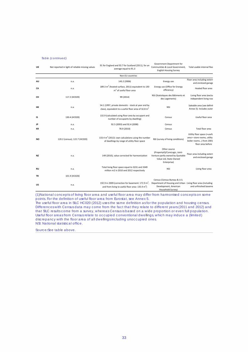
33

Table (continued)

(1)National concepts of living floor area and useful floor area may differ from harmonised concepts on some points. For the definition of useful floor area from Eurostat, see Annex 5. The useful floor area in SILC HC020 (2012) uses the same definition as for the population and housing census. Differences with Census data may come from the fact that they relate to different years (2011 and 2012) and that SILC results come from a survey, whereas Census is based on a wide proportion or even full population. Useful floor areas from Census relate to occupied conventional dwellings, which may induce a (limited) discrepancy with the floor area of all dwellings including unoccupied ones. NSI: National statistical office.

Source:See table above.

UK Not reported in light of reliable missing values91 for England and 93.7 for Scotland (2011), for an

average equal to 91.3

Government Department for Communities & Local Government,

English Housing SurveyTotal usable internal floo

AU n.a. 143.2 (2006) Energy useFloor area including extern

and enclosed garage

CA n.a.189.3 m2 (heated surface, 2011) equivalent to 130

m2 of useful floor areaEnergy use (Office for Energy

efficiency)Heated floor area

CH 117.2 (HC020) 99 (2014)NSI (Statistiques des Bâtiments et

des Logements)Living floor area (exclud independent living room

HK n.a.54.1 (1997, private domestic - stock at year end by class), equivalent to a useful floor area of 32.8 m2 NSI

Saleable area (see definit Annex 5): includes outer

IS 130.4 (HC020)132.9 (calculated using floor area by occupant and

number of occupants by dwelling)Census Useful floor area

JP n.a. 92.5 (2003) and 92.4 (2008) Census

KR n.a. 78.9 (2010) Census Total floor area

NO 120.2 (census); 122.7 (HC020) 133.4 m2 (2012): own calculations using the number of dwellings by range of utility floor space

NSI (survey of living conditions)

Utility floor space (=usefu area + store rooms, utility boiler rooms…) from 2001

floor area before

NZ n.a. 149 (2010), value corrected for harmonization

Other source (PropertyIQ/CoreLogic, Joint-

Venture partly owned by Quotable Value Ltd, State-Owned

Enterprise)

Floor area including extern and enclosed garage

RU n.a.Total living floor space equal to 3231 and 3349

million m2 in 2010 and 2012 respectivelyNSI Living floor area

TR 101.9 (HC020)

US n.a.192.9 in 2009 (correction for basement: 172.9 m2,

and from living to useful floor area: 135.9 m2)

Census (Census Bureau & U.S. Department of Housing and Urban

Development, American Household Survey)

Living floor area (including and unfinished baseme

Non-EU countries

34

Table A1.3: Households' dwelling assets compared to total sectors' (%)

(1)Some countries of the sample are not covered in this table: BG, IE, ES, HR, CY, MT, RO, IS, NO, CH, TR, HK, NZ and RU. Averages and medians are calculated over the whole available period, for some countries since 1970 (not displayed in this table).

Source: OECD, own calculations, for countries for which information is available.

BE CZ DK DE EE EL FR IT LV LT LU HU NL AT PL PT SI SK FI SE UK AU CA JP KR US

1995 96.4 73 69.3 82.2 98.6 81.5 89.4 85.5 97.2 94.7 72.3 83.2 52 90.8 84.4 59.5 94.5 85.9 84.9 95.1 96.5

1996 96.3 73.6 69.8 82.5 98.7 81.1 89.4 84.6 97.1 95.1 72.8 83.1 51.4 90.8 83.8 61.4 94.5 86.2 85.3 95 96.5

1997 96.3 74.2 69.9 82.7 98.7 80.7 89.5 84.7 97 95.2 73.5 83.2 50.9 90.8 83.9 62.7 91.5 94.8 86.5 85.4 95 96.6

1998 96.4 74.6 70 83 98.8 80.3 89.5 84.8 97 95.4 74.1 83.3 49.8 90.8 84.2 63.2 92.1 94.8 86.8 85.5 94.9 96.6

1999 96.3 75.5 70.1 83.3 98.9 80.3 89.6 85 97 95.4 74.8 83.4 49.1 90.9 84.6 61.8 93 95.1 87.1 85.7 94.9 96.7

2000 96.1 77.6 70 83.6 94.7 98.9 80.5 89.6 85.2 97 96.2 95.7 75.4 83.6 48.8 90.8 85 81.5 63.4 93.4 95.2 87.4 85.9 94.9 96.7

2001 95.8 78.2 69.9 83.8 94.6 99 80.7 89.7 85.4 97 96.2 95.9 75.9 83.8 49.6 90.7 85.2 81.7 62.2 93.3 95.3 87.6 86.1 94.8 96.7

2002 95.5 79.2 69.8 84.1 94.5 99 80.9 89.7 85.5 97 96.4 96 76.2 84 49.9 90.6 85.8 82 63.2 93.8 95.4 87.8 86.2 94.8 96.8

2003 95.3 79.4 69.8 84.4 94.3 99 81.2 89.7 85.7 97 96.4 96.1 76.8 84.1 49.6 90.6 85.9 82.3 63.4 93.9 95.6 88.2 86.4 94.8 96.8

2004 95 80.2 69.4 84.7 94.3 99.1 81.5 89.6 86.1 97.1 96.5 96.3 77.4 84.2 84.4 90.6 86.4 82.7 65.8 94 95.7 88.5 86.4 94.8 96.8

2005 94.9 80.8 69.1 84.9 94.1 99.1 81.7 89.6 86.6 97.1 96.6 96.3 78 84.4 86 90.6 86.6 83.1 64.5 93.8 95.7 88.8 86.4 94.9 96.9

2006 94.7 81.1 69.1 85.2 94.3 99.2 81.9 89.6 86.7 97.1 96.8 96.4 78.5 84.5 89.1 90.6 86.8 83.5 64.3 94.4 95.7 89 86.4 94.8 96.9

2007 94.5 79.5 68.9 85.4 94.5 99.2 82 89.6 86.7 97 97 96.5 79.1 84.6 89.1 90.5 86.9 83.9 64 94.5 95.8 89.2 86.3 94.9 96.9

2008 94.3 79.2 68.8 85.6 94.7 99.3 82.2 89.7 86.8 97 97.2 96.5 79.5 84.7 88.8 90.4 87 84.3 64.3 94 95.8 89.5 86.3 94.9 96.9

2009 94.1 81.5 67.5 85.7 95 99.2 82.3 89.9 86.8 97 97.3 96.6 79.6 84.8 88.1 90.3 87.1 84.6 63.7 94.5 95.7 89.9 86.3 94.8 96.9

2010 93.9 82.9 66.6 85.9 95.2 99.2 82.2 90.2 86.8 97 97 96.7 79.6 84.9 89.7 90.2 87.3 84.8 62.6 94.8 95.7 90.1 86.3 94.7 96.9

2011 93.6 83.2 66.9 86.1 95.5 99.3 82.1 90.6 86.9 97 97 96.7 79.5 85 90.6 90.1 87.5 85 62.4 95 95.8 90.3 86.4 94.6 96.9

2012 93.4 84 66.7 86.2 95.6 99.3 82.1 90.8 86.8 97.1 97 96.7 79.4 85.1 90.7 91.8 89.9 87.7 85.1 61.6 95 95.8 90.3 86.5 94.6 96.9

2013 93 84.4 66.7 86.4 99.3 82.1 91.1 86.7 97.1 96.9 96.8 79.2 85.1 91.5 91.9 89.7 87.5 85.3 60.9 95.1 95.8 90.4 86.6 94.5 96.9

2014 92.8 84.9 67 86.5 82.1 91.2 96.9 79.1 85.2 87.3 85.5 95.4 95.9 86.5 94.4 96.9

2015 85.1 85.3 85.6 94.4

Average 94.9 79.6 68.8 84.6 94.7 99 81.5 89.9 86 97.1 96.8 96.1 77 84.2 70.5 91.9 90.5 86 83.8 62.9 94 95.4 88.4 86.1 94.8 96.8

Median 95 79.5 69.2 84.8 94.6 99.1 81.6 89.6 86.1 97 96.9 96.3 77.7 84.4 84.4 91.9 90.6 86.5 84.1 63.2 94 95.7 88.5 86.3 94.8 96.9

35

ANNEX 2 Conversion factors for floor areas For countries outside Europe, national sources for floor areas are used usually based on a concept of floor area that differs from the one of useful floor area used by Eurostat. Therefore, some corrective factors based on the TABULA project have been applied. This project, co-funded by the Intelligent Energy Europe (IEE) Programme of the European Union, has developed residential building typologies for energy purposes, incidentally defining some conversions between different concepts of floor areas.(17)

Based on these conversion factors, coefficients are applied to convert different notions of floor area into them into the corresponding concept of conditioned floor area:

• External dimensions (including walls) should be multiplied by 0.85.

• Conditioned living area should be multiplied by 1.1.

• Conditioned useful floor area should be multiplied by 1.4.

Equalling these expressions, different concepts of floor areas are in turn converted into useful floor areas based on the following conversion factors:

• External dimensions (including walls) should be multiplied by 0.85/1.4 (=0.607).

• Conditioned floor area should be multiplied by 1/1.4 (=0.714).

• Conditioned living area should be multiplied by 1.1/1.4 (=0.786).

To confirm the magnitude of these conversion factors, useful floor areas obtained with the conversion of conditioned floor areas by country from Tabula are compared with the results of Eurostat (EU-SILC survey), for two types of dwellings (see Table A2.1). (18) Single-family houses from Tabula are compared with detached houses from Eurostat and terraced houses are compared with semi-detached houses.

(17) See "Typology Approach for Building Stock Energy Assessment", TABULA Calculation Method – Energy Use

for Heating and Domestic Hot Water- Reference Calculation and Adaptation to the Typical Level of Measured Consumption, page 28.

(18) See Table 4 from : EPISCOPE Project Team (2015), Evaluation of the TABULA Database, Comparison of Typical Buildings and Heat Supply Systems from 20 European Countries, December.

36

Table A2.1: Comparison of useful floor areas from Tabula (April 2015, multiplying conditioned floor area by

1/1.4) and from Eurostat (EU-SILC survey, 2012)

(1)Units: number of square metres of useful floor area for (a), (b), (c) and (d). The 20 countries covered by Tabula are BE, BG, CZ, DK, DE, IE, EL, ES, FR, IT, CY, HU, NL, AT, PL, SI, SE, UK and RS (Serbia). EU countries not covered by Tabula are thus: EE, HR, LV, LT, LU, MT, PT, RO and SK, whose limited weights should make the perimeter of Tabula for 20 countries comparable with the one of EU28 and, conversely, NO and RS are covered by Tabula and are not in EU28. Inertia of average surfaces should also make the figures comparable for 2012 and April 2015.

Source: TABULA/EPISCOPE, Eurostat, own calculations

TABULA single family house

(a)

EU-SILC detached house (b)

(a)/(b)TABULA terraced house (c)

EU-SILC semi-detached house (d)

(c)/(d)

EU28 (Eurostat) & 20 countries (TABULA)

110.71 119.1 0.93 127.14 110.7 1.15

Median over all countries 0.9 0.93Average over all countries 0.94 1.15

37

ANNEX 3 Fall back method: price estimates from property advertisements on real estate agents' website

Table A3.1: Coverage, sources, and results

(Continued on the next page)

Country Period

Sample size (total number of dwellings in the country in

parenthesis: source Eurostat for EU countries, 2011 by default)

CoverageWeights / stratification used for

calculationsResults Remarks

BG Oct-17 2744 (3882810)All but one regions (Yambol, thefifth least constructed one in termsof floor area) are covered

Useful floor areas by region,supplied by NSI

Excluding regions for which less than 10 observations are recorded, a figure of 670.3 BGN/m2 is found

(equivalent to 580.6 in 2012).

Concentrating on flats in districtcentres, which would give aperimeter comparable with theone of the NSI ("market prices ofdwellings") gives 959.6(equivalent to 831.1 in 2012, closeto the NSI figure (881.4 BGN/m2))

EE Oct-17 14535 (649746) All regions are coveredSquare metres by region, puttingapart the capital

The weighted average gives 1046.5 €/m2 in October 2017. Results are close using median

values. Weighted median surfaces are consistent with NSI figures for

2011 (72.7 m2 and 70.6 m2

respectively).

IE 2011 11374 (1649408 dwellings in 2011) All counties are covered Number of rooms by county

1768.8 €/m2 (average) and 1721.2 €/m2 (median) without correcting

for floor area. 2462.8 €/m2

(average) and 2396.5 €/m2

(median) correcting for floor area.

Transaction data from NSI. Floorareas correspond to heated floorarea, not to useful floor area.

IE Oct-17 7683 (1697665 dwellings in 2016) All counties are covered Number of rooms by county

2383.3 €/m2 (average) and 2389.2 €/m2 (median) without correcting

for floor area. 3318.3 €/m2

(average) and 3326.5 €/m2

(median) correcting for floor area.

Floor areas usually used in Irelandcorrespond to heated floor area,not to useful floor area.

EL Nov-17 133324 (6371901) 308 municipalities are coveredover 325 (coverage in terms ofdwellings: 99.5%)

Square metres by region 1350.1 €/m2

FR 2012 290174 (27095096)All regions are covered exceptCorsica (representing around 0.8%of dwellings)

Square metres by region2529 €/m2 (average) and 2398.4

€/m2 (median)Transaction data from notaries-INSEE BIEN / PERVAL

HR Feb-14 149000 (1730000) All counties are covered Floor areas of census by county 1205.7 €/m2

CY Oct-17 6249 (431049) All districts are coveredFloor area of occupied dwellings,for rural and urban areas of eachdistrict

The weighted average gives 2411.1 €/m2 and the weighted

median 1857 €/m2 (the discrepancy between the two

figures signalling a potential over-representation of prime goods)

The median value is retained, dueto the potential over-representation of prime goods

38

Source: Real estate web sites (BG: mirela.bg; EE: kinnisvaraportaal-kv-ee.postimees.ee; IE: myhome.ie; EL: en.tospitimou.gr and xe.gr; HR: dogma-nekretnine.com, realestatecroatia.com; CY: aloizou.com.cy and incyprusproperty.com; LV: ee24.com; LT: alio.lt; AT: immobilien.net; PL: domy.pl, oferty.praca.gov.pl and otodom.pl; PT: casa.sapo.pt and idealista.pt; RO: homezz.ro and magazinuldecase.ro; SI: nepremicnine.si21.com; SK: reality.sk; IS: fasteignir.visir.is; CH: homegate.ch; TR: hurriyetemlak.com), own calculations, Eurostat, national censuses for non-EU countries.

SI Oct-17 4024 (534462)All statistical regions and mainmunicipalities are covered

Number of square metres bymunicipality and statistical regions 1193.1 €/m2 (average)

SK Jul-16 25714 (1941176) All regions are coveredNumber of square metres byregion 752.4 €/m2 (average)

Results are different from the onepublished by the central bankbecause this uses transactions asweights. Using the same weights,the two sources would beconsistent.

CH Oct-17 15171 (4300000) All cantons are coveredFloor areas of cantons, puttingapart Geneva and Basel

7608 CHF/m2 (average) and 6833.6 CHF/m2 (median)

IS Oct-172549 (126211 dwellings from

Census 2011)Cities covered represent 96.2% ofdwellings

Floor area by city 289327.1 ISK/m2 (average)

TR Oct-1751018 (19454000 main dwellings

in 2011)

All provinces are covered. Insideprovinces, only 4 cities are notcovered, representing 324000dwellings

Number of rooms by province (26provinces)

2696.3 LT/m2 (average) and 2306.2 LT/m2 (median)

The median value, consistent withthe perimeter from the CentralBank (CBRT) is 12% above

Table (continued)

LV Jul-16 12971 (1018532)

All regions are covered.Stratification has been made with8 groups: the capital (Riga),Jurmala (3rd city of the countryand main city on the coast),Liepaja (other big city on thecoast), big cities except theprevious ones, intermediary cities,big regions, intermediary regionsand small regions.

Number of houses and flats for allareas except Riga and surfaces byquarters of Riga

Mean price: 703.9 €/m2

Prices may be overestimatedcompared to transaction values,due to high unoccupied rates.Besides, stratification may need tobe refined using floor areasinstead of number of dwellings

LT Oct-17 18370 (1374233) All municipalities are coveredNumber of square metres by

municipality682.5 €/m2 (average) and 635.4

€/m2 (median)

MT 2012 3493 (223850)

All regions are covered. Insideregions, only the municipality ofFontana (613 dwellings in 2011)did not register any transaction

Number of rooms by region

1017.3€/m2 for the mean and 949.4€/m2 for the median (for flats

only: 1161.8€/m2 for the mean and 1094.6€/m2 for the median)

Data come from NSI, registeringtransactions and not from realtors.Surfaces for houses may,sometimes, be wrongly filled andinclude external surface

AT Jul-16 25175 (4441408)

All regions are covered. Offersrepresent between 0.14%(Vorarlberg) and 0.98% (Wien) ofthe stock of dwellings, for anaverage of 0.57%

Floor area by region and, forVienna, by area

2828.7 €/m2 (average) and 3125.3€/m2 (median)

PL Jul-16 361345 (12965598)

All regions are covered and maincities are considered separately.The number of offers byregion/city ranges from 761 up to75795, with a median valuearound 4200.

Number of dwellings by region andmain cities

3215.2 PLN/m2 (average) and3715.1 PLN/m2 (median)

Comparisons with transactionsprices, weighted with the share ofhousing in the market stock, fromPolish Central Bank, for Warsaw,the 6 following main cities and the10 following other main cities, giveclose results (these 17 citiesrepresent around 25% of totalstock of dwellings)

PT Oct-17 69776 (5690222 in 2016) All municipalities are coveredNumber of useful square metresby municipality 1385.7 €/m2 (average)

Floor areas may correspond togross or useful floor areas, whichcounterbalances the positive biasof realtors offers compared totransaction price to surface

RO Oct-17 54214 (8722398)All municipalities and towns arecovered

Number of square metres bymunicipality or town

566.9 €/m2 (average) and 610.9 €/m2 (median)

39

ANNEX 4 Comparison of price level estimates from alternative methods and sources Table A4.1: Price level estimates in euro per sqm from different methods and sources, 2016

(1)"NSI" stands for national statistical institute. Figures are converted in euros for 2016 and the surface of census is for main dwellings only. Unless stated, calculations are performed harmonising for floor area to be consistent with the concept of useful floor area. See Tables A1.1, A1.2, A1.5 for sources and methods.

Source: See table 3.1 and references found in the table above (column 3)

CountryBaseline method

Fall back method Surveys

BE 2079.6 2195.3 (source: Dujardin et al. (2015)) 2171.6 (HFCS, 2nd wave)

BG 306.8 (439.3 for flats in district centres)491.8 (NSI, average “market price of dwellings” (flats) in districtcentres)

CZ 685DK 2101.1 2126.5 (Danish Mortgage Banks data)DE 1965.2 2111.5 (source: Dujardin et al. (2015)) 2295.9 (HFCS, 1st wave)

EE 965.91123.4 (NSI, based on the survey “Real Estate Agencies”, harmonizingfor floor area) and 1378.4 (HFCS, 2nd wave)

IE 3001.1 2845.7 3730 (HFCS, 2nd wave)EL 1218.4 1360.4 938.5 (HFCS, 2nd wave)

ES 1499.4 1643.2 (source: Dujardin et al. (2015))1499.4 (Ministry of development, based on appraisals, ProfessionalAssociation of Valuation Companies (ATASA))

FR 2503.5 2504.5 (source: Dujardin et al. (2015)) 2255.1 (HFCS, 1st wave) and 2935.4 (HFCS, 2nd wave)HR 1195.4 1484.7 (NSI: new dwellings sold)

IT 1763.8 1983.5 (source: Dujardin et al. (2015))

1608.1 and 1511.6 (source: Cannari and Faiella (2008), using theSurvey of Household Income and Wealth, the Osservatorio MercatoImmobiliare dell’Agenzia del Territorio and Il ConsulenteImmobiliare); 1907.4 (HFCS, 1st wave) and 2117.1 (HFCS, 2nd wave)

CY 1769.2 1592 (HFCS, 1st wave) and 1573.4 (HFCS, 2nd wave)LV 694 543.5 (HFCS, 2nd wave)LT 565 615.1

LU 4371.3 4828.9 5535.1 and 5554.4 (HFCS, 1st and 2 waves, harmonizing for floor area)

HU 628.2 652.5 (HFCS, 2nd wave)MT 1159.2 1321.8 (HFCS, 2nd wave)NL 2164 2354.7AT 2498.5 2805.5 3530.6 (HFCS, 2nd wave)

PL 653.3 716.8889.9 (NSI, new residential buildings, harmonizing for floor area) and1085.4 (HFCS, 2nd wave)

PT 1166.5 1226.11160.4 (NSI, Survey Inquérito à Avaliação Bancária na Habitação) and1226.6 (HFCS, 2nd wave)

RO 541.9SI 1136.6 1061.4SK 709.1 744.9 805 and 771.9 (HFCS, 1st and 2nd waves)FI 1602 1674 1601.6 (HFCS, 1st wave) and 1810.8 (HFCS, 2nd wave)

SE 2432 2541.32489.1 (average purchase price for one and two-dwellings buildings,source: NSI)

UK 2500.82538.8 (Halifax-financed transactions, existing

homes)

IS 2148.6 1945.3

NO 2640.72925.7 (NSI: freeholders, using average price per m2 for detachedhouses, row houses and multi-dwellings, weighting by stocks of floorareas)

CH 5190 5775.6 (harmonizing for floor area)

TR 890.1 (median: 793.8)696.8 (Central Bank: stratified median price using the appraisal valueof houses from approval of individual loans)

AU 5351.5

CA 2442.12678.8 (Canadian Real Estate Association, sale

prices)2552.2 (National Household Survey, harmonizing for floor area)

HK 29836.3JP 1510NZ 3977.1RU 686.7KR 2438.5

US 14741467.4 (Census, new single-family houses sold, harmonizing for floorarea)

EU countries

Non EU countries

40

Graph A4.1: Price level estimates in euro per sqm (in log) from different methods and sources, 2016

(1)Prices are in euros and in logarithm. A difference by 0.1 point between two sources means a difference by 10%. HK is not represented, because it would be out of scale and has only one source anyway. BG displays an important discrepancy between realtors and survey data because the latter covers only flats in district centres: comparing the two sources in this latter perimeter would lead to a much reduced discrepancy, around 6%. Realtors data for BE, DE, ES, FR and IT are from Dujardin et al. (2015) and for UK and CA are directly from realtors and are represented in yellow.

Source: See Table A.4.1.

ANNEX 5 Definition of statistical concepts

41

Conditioned floor area: floor area based on internal dimensions, measured to the inside surface of external walls. It is generally equal with the heated area or with the air-conditioned area, dependent of which is the bigger one.

Gross disposable income per capita: Calculated as the ratio between gross disposable income of households and non-profit institutions serving households (NPISHs) and total population. Source: national accounts.

Living floor space: The living floor area is obtained by adding to the surface of living rooms (kitchens above 4m2, dining rooms, livings, bedrooms…) the floor area of kitchens smaller than 4m2, bathrooms, toilets, corridors and halls, covered terraces and swimming pools inside dwellings. The floor area is measured inside outer walls, excluding cellars and attics. This definition may vary marginally for non-EU Countries.

Purchasing Power Parity (PPP): Expressed in national currency per current international dollar. The source is World Economic Outlook (WEO, IMF), using primary source information from: OECD, the World Bank, and the Penn World Tables(19).

Saleable area (in the case of Hong-Kong): floor area exclusively allocated to the unit including balconies, verandas, utility platforms and other similar features but excluding common areas such as stairs, lift shafts, pipe ducts, lobbies and communal toilets. It is measured to the exterior face of the external walls and walls onto common parts or the centre of party walls.

Useful floor space: according to Eurostat, useful floor space is defined as the floor space measured inside the outer walls excluding non-habitable cellars and attics and, in multi-dwelling buildings, all common spaces; or the total floor space of rooms falling under the concept of 'room'. A 'room' is defined as a space in a housing unit enclosed by walls reaching from the floor to the ceiling or roof, of a size large enough to hold a bed for an adult (4 square metres at least) and at least 2 metres high over the major area of the ceiling. The useful floor area in SILC HC020 (2012) uses the same definition as for census.

(19) For further information see Box A2 in the April 2004 World Economic Outlook, Box 1.2 in the September 2003 WEO for a

discussion on the measurement of global growth and Box A.1 in the May 2000 WEO for a summary of the revised PPP-based weights, and Annex IV of the May 1993 WEO. See also Anne Marie Gulde A.-M. and Schulze-Ghattas M. (1993), Purchasing Power Parity Based Weights for the WEO, in Staff Studies for the World Economic Outlook (Washington: IMF), pp. 106-123, December.

42

Table A5.1: Price level estimates (€/m2)

Source: See Table 3.2 for level estimates and Eurostat, BIS and OECD for house price indices series and exchange rates.

BE BG CZ DK DE EE IE EL ES FR HR IT CY LV LT LU HU MT NL AT PL PT RO SI SK FI SE UK IS NO CH TR AU CA HK JP NZ RU KR US

1980 426,6 404,6 857,0 460,8 214,2 559,3 454,0 430,1 497,1 303,2 501,7 358,4 311,6 978,3 331,6 602,4 316,1

1981 399,4 382,9 961,8 562,1 217,9 594,4 567,8 442,6 465,2 370,1 481,4 367,3 368,2 1278,2 747,1 460,4 744,5 307,6 400,5

1982 354,4 366,2 1032,5 597,3 195,5 596,9 623,3 393,7 436,8 405,5 409,2 354,9 371,3 1356,0 754,3 469,4 842,2 402,1 464,1

1983 342,8 441,2 1054,7 611,6 218,6 592,8 649,7 389,8 445,5 521,9 438,9 417,3 424,5 1511,1 854,9 574,3 1045,8 463,7 563,9

1984 360,5 521,5 1043,8 650,2 248,3 622,4 667,7 423,4 445,6 606,8 467,9 426,8 479,7 1566,6 1021,9 628,7 1162,6 443,6 686,5

1985 366,5 612,7 1055,0 658,8 245,9 655,0 626,3 448,2 456,7 608,8 460,9 459,9 553,8 1641,6 742,8 499,7 1190,0 425,6 576,2

1986 396,1 692,7 1112,8 632,5 274,3 668,5 663,5 515,3 502,2 594,9 455,7 443,4 617,7 1844,6 642,1 488,0 1272,2 409,4 510,3

1987 422,2 634,7 1111,9 615,7 379,4 704,9 667,0 557,3 532,1 661,7 493,7 538,8 646,6 2052,8 606,1 493,3 1477,5 492,0 446,1

1988 451,8 635,1 1121,5 670,2 501,8 768,5 748,3 638,9 549,9 465,7 940,7 614,0 738,4 709,2 2231,9 977,1 703,4 1690,3 590,9 522,3

1989 526,3 642,4 1188,5 732,9 627,2 883,2 889,9 782,5 601,8 527,5 1159,0 706,3 769,7 646,2 2404,1 1103,7 801,2 1552,4 580,3 538,7

1990 587,7 594,0 1270,8 835,6 727,8 956,9 1028,2 901,5 609,1 594,2 1074,1 762,6 797,9 589,6 2537,7 960,3 682,9 1639,5 531,4 487,7

1991 616,4 598,2 1332,3 860,9 838,0 1006,1 1189,5 979,5 627,5 720,8 823,3 839,7 777,4 553,7 2390,7 987,9 727,0 1887,2 485,2 502,6

1992 686,2 616,0 1461,9 904,6 773,2 1024,2 1179,6 1127,5 710,1 820,2 598,7 662,7 669,7 502,7 2357,1 1005,2 753,3 2012,7 515,1 570,5

1993 720,7 611,8 1548,1 867,6 671,9 1023,4 1156,7 1109,4 779,7 749,2 535,1 542,1 696,0 507,2 2384,9 1102,9 797,5 2333,3 631,8 634,2

1994 788,9 693,3 1637,8 904,1 663,5 1021,8 1092,4 1161,7 870,6 770,9 628,5 574,2 685,4 578,8 2440,7 1185,5 707,7 2317,5 746,8 594,6

1995 834,5 765,1 1680,9 931,2 697,3 1033,8 1055,9 1178,9 928,3 780,2 617,6 607,6 641,1 621,7 2501,9 1077,7 650,8 2063,0 779,9 570,9

1996 822,7 829,6 1605,1 1113,0 690,3 1023,5 1193,3 1213,1 992,5 795,1 640,3 617,5 763,7 698,8 2119,6 1218,8 678,7 1882,5 977,2 616,4

1997 828,7 90,9 915,3 1552,9 1232,6 867,6 687,8 1011,0 1215,9 1236,2 1089,1 798,8 730,8 650,5 918,7 777,1 2155,3 1179,6 754,4 1884,2 968,3 933,1 719,5

1998 890,7 104,5 1008,1 1555,0 1499,8 939,0 724,1 1040,7 1219,0 1293,9 1221,3 841,3 811,1 655,6 967,8 789,7 2133,5 1127,4 652,5 2004,1 816,2 1130,2 713,9

1999 954,0 105,4 1076,9 1556,6 1822,3 1020,7 799,2 1111,3 1231,8 211,4 1377,1 1420,4 916,9 883,6 794,5 1217,7 963,9 2134,1 1489,2 828,9 10923,7 2509,6 951,5 1376,4 879,8

2000 1005,8 104,6 247,2 1143,9 1563,8 2198,5 1093,9 867,8 1209,5 736,9 1280,0 213,8 206,0 1477,0 374,3 1679,0 1389,5 987,9 934,2 856,8 1394,0 999,7 1096,0 2249,8 1483,2 904,2 10524,0 2320,6 868,2 1354,2 1013,8

2001 1054,2 105,4 296,8 1215,2 1565,3 2530,0 1251,4 952,6 1303,7 773,9 1354,5 222,1 245,1 1685,3 418,5 1839,4 1400,1 1041,7 919,4 878,1 1545,9 912,2 1213,1 2332,1 1601,1 939,4 9760,0 2056,6 880,2 1426,4 1144,5

2002 1121,3 95,6 338,4 1260,3 1543,6 2642,5 1424,7 1099,2 1417,7 802,9 1515,8 1376,4 295,3 264,1 1827,5 450,1 1956,2 1409,1 1047,6 977,7 949,3 1679,3 1036,5 1392,0 2377,0 1770,5 863,4 7290,2 1805,0 1029,9 258,8 1553,7 1029,7

2003 1199,5 106,6 363,2 1297,4 1549,7 3021,2 1501,6 1288,1 1586,2 810,5 1609,0 1362,2 330,3 289,8 2032,5 507,6 2004,3 1412,6 1059,2 743,3 1039,0 1019,6 1794,4 1098,6 1223,7 2247,2 2308,0 953,6 5353,1 1559,7 1278,9 287,4 1398,8 920,6

2004 1303,6 157,1 388,0 1414,8 1526,3 383,2 3358,6 1536,4 1508,0 1826,7 897,6 1708,2 1519,9 327,0 313,2 2316,6 589,6 2084,4 1386,1 1066,3 804,7 1122,6 1122,6 2006,4 1302,7 1377,3 2351,7 2359,8 1020,5 6280,4 1416,3 1524,6 359,5 1504,5 934,3

2005 1468,8 214,5 413,9 1658,8 1544,3 508,5 3683,4 1703,8 1712,3 2106,7 1038,5 1838,5 1633,4 406,3 393,6 2580,9 642,3 2183,7 1455,1 1090,8 921,7 344,1 1214,1 1182,9 2306,0 1895,0 1537,9 2419,3 2604,4 1318,1 8574,5 1354,6 1907,6 494,2 1809,9 1191,5

2006 1612,0 246,1 470,2 2059,2 1538,8 760,2 4231,0 1929,3 1941,9 2362,0 1226,3 1944,0 1812,2 629,6 505,2 2868,3 770,0 2277,0 1515,2 1113,0 1076,1 441,8 1298,7 1381,3 2537,9 1772,5 1694,8 2486,0 2687,2 1322,4 7717,2 1163,3 1944,2 716,2 1867,1 1130,3

2007 1737,6 317,3 579,2 2113,8 1505,4 918,1 4546,9 2044,1 2132,4 2498,3 1377,7 2041,0 2000,6 859,0 638,2 3068,7 669,2 931,7 2387,2 1585,9 1128,3 1330,3 584,2 1375,3 1488,4 2554,2 1965,0 1974,8 2555,8 2958,5 1560,2 7688,9 1095,8 2122,5 997,1 1825,4 1011,5

2008 1814,2 396,5 647,6 2006,6 1525,8 829,8 4231,3 2078,5 2101,8 2518,7 1412,8 2094,9 2113,5 853,9 695,5 3171,4 651,8 1034,9 2439,6 1601,8 768,8 1171,0 914,9 1423,5 767,9 1386,2 1306,8 1877,9 1128,5 1594,6 2955,7 2541,8 1398,6 9528,9 1442,3 1595,6 1081,2 1464,6 983,4

2009 1805,7 315,6 632,0 1768,4 1538,8 521,1 3420,9 2001,2 1963,0 2362,8 1352,3 2084,6 1974,8 534,6 487,3 3134,7 609,1 990,1 2330,9 1665,3 756,2 1160,2 662,1 1288,6 670,0 1406,1 1426,8 1835,1 962,9 1909,0 2972,0 3349,5 1527,7 9257,0 1287,0 1917,7 1028,2 1630,2 894,1

2010 1862,4 283,5 655,9 1815,1 1555,4 550,6 2959,2 1908,1 1928,3 2476,3 1252,5 2067,9 1861,7 475,9 451,3 3304,6 578,4 1000,8 2290,6 1768,0 751,6 1169,1 608,5 1290,3 643,2 1494,8 1762,1 2001,8 1092,0 2198,1 3623,8 796,3 4558,5 1889,2 12389,1 1600,1 2250,8 1177,5 1852,7 935,1

2011 1937,2 267,9 638,1 1788,9 1609,2 597,4 2453,7 1803,8 1781,0 2620,0 1229,0 2083,9 1831,9 533,0 481,2 3426,2 493,6 987,2 2245,4 1878,5 670,7 1111,7 526,0 1325,3 633,5 1542,4 1817,0 2032,8 1106,3 2388,2 3964,9 723,8 4605,1 1999,1 15443,3 1736,3 2341,9 911,3 1943,8 925,5

2012 1980,6 262,8 644,7 1734,2 1664,8 640,9 2123,6 1593,5 1517,7 2605,9 1206,5 2025,2 1776,0 550,2 480,0 3570,1 511,5 1017,3 2094,5 2015,9 708,3 1033,1 485,7 1233,9 616,4 1579,7 1909,1 2089,0 1106,4 2690,9 4186,4 821,7 4594,2 2107,8 17196,1 1517,8 2558,4 1085,6 2097,1 934,4

2013 2003,9 257,0 591,2 1802,3 1716,7 709,1 2150,2 1420,6 1379,3 2555,6 1148,4 1909,6 1703,3 583,6 485,9 3747,9 490,5 1013,1 1968,9 2120,2 664,2 1013,7 481,6 1169,2 622,0 1597,9 1950,8 2097,4 1253,6 2459,6 4239,8 722,3 4037,5 1935,9 19324,3 1211,1 2670,7 1002,7 2010,5 958,2

2014 1992,7 260,7 598,9 1873,8 1770,5 806,4 2505,7 1314,5 1383,6 2515,7 1125,7 1826,1 1673,2 618,6 517,1 3912,4 481,1 1039,0 1984,9 2194,6 652,0 1056,7 470,5 1092,0 630,7 1592,3 2012,7 2425,1 1396,4 2336,9 4446,1 847,4 4579,4 2126,3 23256,2 1225,6 3071,0 636,8 2236,4 1144,5

2015 2026,1 267,9 639,0 1999,6 1853,9 861,7 2792,8 1248,9 1433,1 2478,5 1095,9 1778,1 1649,0 597,8 536,0 4123,5 543,3 1099,3 2055,6 2302,1 663,4 1089,0 479,5 1100,8 664,6 1592,3 2327,2 2726,9 1650,0 2334,6 5062,5 865,1 4970,0 2084,8 29986,0 1390,7 3347,0 578,0 2378,2 1345,6

2016 2079,6 286,7 685,0 2101,1 1965,2 902,7 3001,1 1218,4 1499,4 2503,5 1117,2 1763,8 1653,5 648,6 565,0 4371,3 628,2 1159,2 2164,0 2498,5 653,3 1166,5 506,4 1136,6 709,1 1602,0 2432,0 2500,8 2148,6 2640,7 5190,0 831,9 5351,5 2442,1 29836,3 1510,0 3977,1 686,7 2438,5 1474,0

2017 2156,0 311,6 809,4 2190,8 2043,0 952,3 3328,4 1206,2 1592,2 2585,6 1178,6 1756,7 1690,6 705,9 615,3 4617,5 680,7 1215,7 2338,5 2630,4 716,4 1274,3 523,3 1228,1 750,9 1625,2 2511,0 2526,0 2446,5 2559,7 4855,7 749,4 5514,9 2582,9 30381,4 1416,0 613,3 2448,3 1382,3

43

Table A5.2: Price level estimates, purchasing power parity (national currency divided by PPP index using implied conversion rate compared to the US (US: PPP=1)

Source: See Table 3.2 for level estimates and Eurostat, BIS and OECD for house price indices series and exchange

BE BG CZ DK DE EE IE EL ES FR HR IT CY LV LT LU HU MT NL AT PL PT RO SI SK FI SE UK IS NO CH TR AU CA HK JP NZ RU KR US

1980 518.514 469.044 1233.96 740.908 401.216 645.907 797.237 536.161 607.717 342.591 430.485 378.479 405.691 1227.39 678.787 462.172 4070.58 664.644 392.161 1340.86 413.96

1981 510.334 441.482 1383.25 832.225 395.942 701.603 982.675 561.965 566.917 384.736 452.558 389.699 432.452 1399.91 775.35 524.877 4926.78 783.362 466.573 1351.62 434.617

1982 485.019 415.998 1416.85 809.704 382.792 702.397 990.213 576.656 508.437 444.475 446.139 392.318 454.067 1454.73 761.21 483.905 4126.06 881.699 584.317 1421.07 449.117

1983 469.709 489.21 1430.54 816.927 422.817 700.165 965.135 558.892 526.544 516.452 423.42 432.164 471.572 1535.83 769.312 502.263 3503.95 951.676 613.572 1669.46 466.52

1984 470.744 551.734 1419.58 822.205 427.308 702.99 927.128 575.838 533.812 552.167 416.967 464.836 524.611 1619.75 839.047 499.881 3158.06 1002.53 665.941 1874.22 486.704

1985 471.064 638.982 1419.33 806.077 446.317 710.744 892.394 626.278 542.131 564.747 420.093 493.867 621.105 1714.46 906.37 525.902 3420.6 1046.65 678.809 1989.98 511.583

1986 489.617 711.56 1406.18 796.728 475.854 722.323 870.965 711.649 578.952 572.244 430.657 547.6 835.451 1799.63 931.836 605.463 3775.39 1078.27 671.605 2076.31 546.267

1987 525.206 645.05 1404.5 784.717 637.305 774.498 891.446 787.605 623.882 627.41 475.661 622.586 858.171 1927.83 943.287 687.904 4396.86 1190.39 692.838 2036.31 581.405

1988 574.794 649.566 1456.5 852.588 782.676 859.962 976.387 917.742 677.473 1035.97 813.277 545.084 776.189 878.889 2231.4 1096.28 800.32 5065.48 1295.97 733.705 2275.45 612.471

1989 649.118 638.297 1526.03 911.723 937.478 969.653 1126.79 1097.16 740.578 1148.86 970.03 622.924 894.701 808.94 2525.73 1320.98 896.852 5900.4 1421.35 773.307 2543.06 644.777

1990 723.915 596.542 1654.33 1069.15 1048.18 1064.97 1283.94 1267.07 770.931 1228.61 904.047 660.232 848.014 749.579 2498.42 1325.51 874.502 6336.32 1632.14 821.594 2806.67 664.829

1991 758.249 608.314 1557.95 1109.55 1155.86 1128.6 1429.16 1388.95 792.608 1367.42 792.031 672.989 810.372 710.955 2408.76 1384.78 914.371 8182.61 1708.79 825.575 2923.02 673.909

1992 799.354 602.081 1588.84 1124.63 1092.04 1105.23 1608.43 1509.43 856.905 1442.9 666.383 616.313 772.517 694.934 2307.5 1420.64 946.064 10623.5 1653.02 834.995 2593.53 690.819

1993 829.208 606.925 1636.93 1115.49 1055.53 1097.52 1660.87 1438.88 934.29 1418.92 610.78 547.884 757.259 701.981 2188.02 1475.45 976.937 10931.5 1610.78 870.988 2413.73 707.545

1994 882.352 685.092 1706.43 1176.22 1047.45 1108.58 1616.8 1445.8 1029.46 1387.14 649.333 570.51 785.292 812.708 2205.78 1540.83 1016.79 12971.5 1602.51 1002.68 2243.27 731.341

1995 904.548 742.993 1733.53 1208.07 1069.77 1108.04 1564.39 1446.12 1075.36 1363.22 612.857 562.63 787.223 864 2149.31 1548.01 967.048 11873.7 1618.47 1097.28 2138.7 750.3

1996 936.835 820.854 1732.62 1326.63 1072.59 1122.69 1580.91 1524.58 1198.45 1375.63 659.369 571.672 798.678 919.787 2070.99 1559.25 967.603 12441.2 1625.68 1207.06 2103.62 772.4

1997 967.055 562.908 912.881 1726.24 1487.92 1298.18 1082.8 1127.33 1621.68 1637.34 1329.54 1395.91 771.421 610.376 876.365 1018.8 2041.5 1631.02 997.414 16694.8 1622.2 1296.38 2117 794.449

1998 1021.45 491.333 993.298 1716.32 1747.97 1426.22 1117.39 1152.44 1597.66 1720.61 1460.94 1421.18 833.624 670.415 975.378 1152.29 2047.83 1753.72 996.989 11966.1 1612.84 1274.1 1857.19 832.906

1999 1104.15 469.432 1058.74 1735.29 2068.42 1522.08 1220.21 1247.26 1614.42 613.285 1765.57 1701.04 1520.52 912.789 737.559 1089.26 1218.88 2074.73 1893.34 1021.01 10817.4 1607.28 1314.61 1883.85 883.872

2000 1166.8 444.617 621.609 1119.47 1795.38 2389.64 1695.99 1308.85 1366.68 1689.11 1682.04 541.196 559.366 1805.67 672.91 1984.69 1606.4 1619.52 971.092 826.112 1253.62 861.881 1251.72 2090.83 2009.2 1043.54 10262.1 1604.21 1308.86 1940.8 943.303

2001 1225.82 430.134 663.671 1182.23 1817.96 2643.64 1916.39 1413.37 1476.44 1688.09 1768.32 542.672 646.119 2098.72 736.059 2133.86 1624.28 1682.88 946.84 889.684 1375.24 859.242 1346.42 2136.04 2208.08 1099.24 9383.51 1585.99 1305.78 1990.69 1008.65

2002 1300.78 383.745 738.993 1215.09 1796.94 2674.61 2142.48 1590.77 1598.31 1747.79 1943.34 2170.53 770.058 691.198 2273.06 817.918 2222.9 1642.31 1649.74 1012.07 946.012 1585.45 867.194 1460.18 2171.25 2586.83 1191.8 8767.63 1546.98 1449.71 1393.45 2287.49 1079.85

2003 1393.12 426.33 820.853 1260.01 1816.75 3006.18 2227.83 1829.7 1790.34 1768.8 2039.26 2122.42 916.173 778.941 2509.23 945.202 2274.97 1655.99 1644.78 1189.85 1094.8 1010.26 1830.24 984.957 1471.9 2219.99 3013.07 1275.24 8375.03 1504.54 1746.67 1531.7 2460.38 1162.67

2004 1524.71 610.756 815.356 1381.56 1810.59 939.228 3416.66 2272.78 2117.91 2082.85 1945.7 2167.76 2335.2 906.951 842.052 2852.94 1117.01 2398.65 1642.28 1660.93 1298.62 1208.35 1130.54 2050.15 1092.21 1574.25 2357.7 3186.39 1373.15 11309.1 1467.78 2027.52 1673.65 2471.52 1272.57

2005 1736.12 808.725 853.833 1629.59 1883.31 1213.63 3762.39 2542.91 2381.53 2432.71 2161.25 2366.19 2481.43 1042.82 1022.31 3151.28 1214.23 2542.15 1734.38 1696.45 1510.11 817.83 1335.66 1269.66 2303.67 1425.96 1617.49 2503.21 3195.25 1482.89 13789.5 1456.31 2339.76 1786.57 2551.44 1405.62

2006 1919.05 896.483 941.062 2041.43 1930.68 1716.08 4321.8 2870.99 2678.5 2752.93 2522.03 2527.91 2771.4 1483.67 1266.14 3370.51 1461.02 2666.32 1827.78 1731 1778.6 956.457 1459.17 1445.12 2484.26 1584.28 1742.35 2684.68 3354.68 1664.54 14398.1 1469.32 2604.14 2369.21 2809.36 1488.54

2007 2083.48 1068.17 1113.81 2100.94 1907.96 1908.71 4702.07 3019.32 2921.06 2915.21 2786.82 2661.08 3045.01 1729.98 1512.26 3648.88 1478.96 1764.52 2808.49 1919.98 1749.27 2166.69 1252.47 1543.49 1622.72 2734.49 1705.78 1953.96 2847.92 3645.32 1844.73 16005.1 1504.34 2841.52 3087.64 3098.01 1489.01

2008 2175.32 1258.88 1255.88 1950.77 1951.12 1636.61 4501.41 2999.35 2875.31 2925.27 2765.92 2717.15 3135.8 1596.54 1531.99 3700.57 1470.36 1941.63 2856.72 1939.21 1832.11 1818.27 2451.91 2263.08 1465.49 1540.27 1618.57 2588.52 1651.45 1784.82 2957.66 3631.62 1907.97 18761.8 1559.37 2665.74 3319.7 3285.57 1368.64

2009 2165.11 969.078 1185.64 1720.94 1950.26 1029.82 3861.02 2834.62 2700.11 2763.46 2576.13 2672.58 2951.94 1116.96 1120.32 3636.53 1349.34 1823.48 2739.01 1994.4 1729.24 1795.95 1810.66 1997.87 1303.55 1545.21 1640.46 2341.6 1363.23 1933.22 2979.19 3794.73 1911.53 19093.3 1489.14 2619.03 3260.4 3225.64 1288.1

2010 2219.83 871.886 1196.12 1734.88 1976.41 1083.95 3493.76 2718.05 2678.19 2899.62 2422.66 2675.16 2762.21 1013.43 1025.73 3742.44 1302.88 1796.79 2701.18 2125 1656.92 1821.05 1637.25 2044.81 1258.66 1657.24 1775.63 2464.98 1268.58 1998.48 3088.74 1770.1 4070.7 2049.51 23982.9 1558.6 2628.24 3130.57 3234.57 1249.46

2011 2308.94 793.888 1221.82 1729.59 2065.73 1139.99 2967.02 2602.87 2526.2 3100.62 2436.4 2713.41 2721.96 1073.82 1059.86 3781.7 1255.72 1769.14 2698.77 2263.25 1640.14 1770.26 1408.22 2120.45 1247.12 1700.6 1835.99 2432.67 1315.65 2063.76 3344.74 1791.72 3877.58 2125.34 28418.3 1619.11 2637.76 2194.3 3408.87 1197.49

2012 2357.81 781.088 1208.45 1674.11 2148.15 1206.91 2561.66 2350.26 2190.04 3105.96 2404.63 2647.35 2638.9 1088.03 1048.14 3914.61 1191.2 1819.86 2529.58 2423 1574.25 1682.58 1301.3 1999.86 1218.17 1722.68 1872.01 2449.43 1386.93 2171.49 3576.68 1858.89 3959.44 2242.07 31667 1646.85 2821.23 2357.52 3478.11 1232.88

2013 2399.83 781.786 1210.62 1751.83 2209.43 1310.76 2609.41 2178.88 2013.52 3071.62 2328.75 2506.1 2600.39 1160.27 1065.55 4104.98 1145.81 1805.92 2383.65 2548.34 1525.24 1640.32 1275.73 1894.95 1243.95 1727.41 1985.52 2505.21 1463.09 2238.49 3741.77 1963.53 4236.13 2299.76 37138.9 1706.56 3028.82 2359.45 3466.4 1321.47

2014 2412.49 802.942 1231.99 1831.55 2278.62 1496.12 3108.77 2093.1 2061.93 3060.44 2331.7 2415.45 2639.19 1232.37 1141.47 4289.89 1175.56 1842.12 2441.49 2634.55 1560.09 1729.51 1250.99 1787.26 1284.62 1723.25 2172.26 2706.21 1551.63 2332.99 3939.61 2088.62 4683.34 2417.28 38961.8 1733.95 3208.47 2263.49 3562.56 1389.51

2015 2452.96 816.309 1279.61 1966.57 2358.67 1595.8 3262.58 2030.74 2145.43 3015.21 2289.62 2355.06 2659.69 1202.9 1193.78 4511.49 1318.91 1925.23 2534.7 2730.82 1589.18 1764.94 1267.22 1804.63 1370.26 1708.45 2433.82 2888.04 1601.01 2574.83 4108.8 2243.32 5206.64 2595.88 43894.8 1757.41 3618.05 2144.93 3615.63 1464.97

2016 2508.61 865.525 1372.25 2085.82 2497.02 1665.44 3547.41 2023.97 2268.31 3071.83 2341.38 2348.67 2723.98 1318.29 1261.06 4906.09 1500.07 2023.07 2688.17 2967.28 1632.5 1884.49 1332.5 1869.41 1489.71 1728.15 2635.46 3067.5 1743.02 2822.15 4251.39 2357.88 5500.74 2873.05 42148.8 1814.36 4076.08 1992.4 3655.08 1553.75

2017 2600.75 946.42 1539.79 2183.13 2612.55 1722.07 4019.83 2027.21 2427.17 3203.94 2444.51 2364.38 2831.76 1417.42 1340.61 5241.2 1598.7 2114.31 2930.45 3131.38 1692.45 2068.68 1370.23 2016.55 1584.18 1768.49 2796.78 3206.27 2110.61 2918.63 4397.98 2389.33 5864.99 3204.94 48647.6 1899.14 1852.3 3656.14 1657.75

44

Table A5.3: Price level estimates (national currency/m2)

Source: See Table 3.2 for level estimates and Eurostat, BIS and OECD for house price indices series and exchange rates.

BE BG CZ DK DE EE IE EL ES FR HR IT CY LV LT LU HU MT NL AT PL PT RO SI SK FI SE UK IS NO CH TR AU CA HK JP NZ RU KR US

1980 437.1 3190.9 1124.1 403.8 133.6 506.4 285.4 440.7 629.6 256.6 2876.1 196.8 2108.0 2264.5 624.5 517.2 16945.8 159909.4 328.6 635659.8 414.0

1981 413.4 3040.5 1202.0 490.2 138.2 562.0 382.3 458.0 566.4 294.3 2890.5 208.1 2319.7 2494.6 718.7 592.6 20761.5 177422.1 405.0 683261.8 434.6

1982 398.2 2971.5 1214.2 525.5 142.8 593.5 426.8 442.3 503.9 348.9 2897.7 213.0 2534.6 2618.5 744.5 559.9 17969.0 191309.3 531.7 720206.0 449.1

1983 391.7 3609.9 1217.4 566.1 170.4 623.8 460.4 445.4 512.9 421.9 2908.5 238.1 2708.7 2726.1 787.0 591.7 15347.3 200529.5 584.7 853417.0 466.5

1984 399.7 4166.1 1191.0 590.3 183.3 648.2 472.8 469.3 509.3 472.7 2980.5 260.3 3090.5 2879.9 877.6 588.4 14643.9 207011.2 659.9 966159.4 486.7

1985 405.6 4875.4 1178.0 597.3 201.7 669.5 481.9 496.0 510.1 493.0 3095.7 283.0 3729.7 3020.9 967.1 620.0 16199.9 212058.4 753.5 1033727.0 511.6

1986 424.5 5445.6 1181.2 614.3 232.7 700.7 495.6 552.2 534.4 513.3 3304.4 321.4 4890.7 3201.5 1034.3 721.1 18182.3 217599.0 830.8 1109653.0 546.3

1987 451.7 5042.4 1171.4 608.2 320.6 750.5 524.2 596.2 559.6 572.2 3729.2 375.4 5252.9 3418.0 1094.2 837.2 22424.0 233876.9 972.7 1113705.0 581.4

1988 488.0 5099.7 1191.4 662.5 400.7 831.6 591.7 690.1 585.3 398.8 771.0 4405.9 478.9 5450.9 3929.5 1340.8 983.6 27156.0 247546.7 1099.8 1287847.0 612.5

1989 555.6 5063.0 1230.0 715.7 494.1 931.8 697.5 826.2 624.3 471.0 943.8 5233.8 571.7 5100.4 4430.1 1672.4 1111.2 34275.5 266846.0 1168.5 1469138.0 644.8

1990 614.6 4682.3 1326.8 814.7 571.3 1013.8 817.9 942.7 636.8 541.8 892.3 5853.0 564.8 4730.6 4419.7 1698.0 1080.0 38176.4 303188.7 1233.2 1721656.0 664.8

1991 640.7 4743.0 1386.6 837.7 653.1 1066.5 947.5 1018.1 653.1 646.8 768.3 6256.1 556.7 4438.5 4345.4 1742.0 1127.4 52074.2 316195.4 1203.7 1899849.0 673.9

1992 683.4 4666.1 1461.7 853.6 644.3 1041.1 1088.9 1123.0 707.8 727.2 637.7 5665.8 534.6 4214.8 4155.8 1768.7 1157.0 72643.6 304042.9 1212.4 1775733.0 690.8

1993 719.8 4621.1 1532.2 871.2 641.8 1026.2 1141.0 1107.9 766.1 736.4 581.5 5039.4 525.5 4254.0 3940.6 1814.8 1182.1 79308.4 291033.8 1262.1 1714272.0 707.5

1994 765.9 5187.5 1595.5 912.7 646.3 1024.3 1126.9 1127.7 843.1 753.2 616.2 5269.8 539.5 4814.5 3937.3 1879.8 1222.2 97973.9 284258.7 1433.8 1686399.0 731.3

1995 800.5 5581.4 1619.1 970.1 668.6 1015.0 1135.7 1130.9 888.2 764.8 593.9 5284.2 543.2 5167.6 3784.9 1902.5 1165.3 91486.7 279724.6 1568.0 1684254.0 750.3

1996 817.9 6177.7 1597.5 1053.3 681.1 1023.9 1179.4 1205.9 983.9 777.2 626.4 5327.4 563.1 5632.8 3584.9 1917.9 1165.0 99679.2 274564.5 1729.7 1696167.0 772.4

1997 837.5 179.6 6890.4 1569.1 1208.2 794.5 691.9 1019.1 1219.5 1249.3 1100.9 805.4 735.9 5680.2 612.6 6305.3 3460.3 1994.7 1193.9 139084.6 270721.6 1834.4 1746431.0 794.4

1998 890.7 204.4 7509.3 1555.0 1499.8 908.5 724.1 1040.7 1219.0 1293.9 1221.3 841.3 811.1 6220.1 682.8 7005.9 3430.1 2141.3 1178.4 99821.1 266150.5 1802.8 1585630.0 832.9

1999 954.0 206.1 8015.7 1556.6 1822.3 989.4 799.2 1111.3 1231.8 245.9 1377.1 1420.4 916.9 883.6 6803.2 757.0 7785.0 3425.4 2296.6 1210.9 85241.2 257814.8 1841.8 1565381.0 883.9

2000 1005.8 204.5 8664.6 8537.1 1563.8 2198.5 1093.9 867.8 1209.5 5585.9 1280.0 175.3 222.1 1477.0 355.3 1679.1 1389.5 987.9 934.2 7566.4 870.0 78775.9 9023.7 3426.9 2487.4 1262.7 76381.0 248116.2 1833.7 1593967.0 943.3

2001 1054.2 205.2 9486.5 9037.0 1565.3 2530.0 1251.4 952.6 1303.7 5687.2 1354.5 175.8 250.0 1685.3 389.4 1839.4 1400.1 1041.7 919.4 8167.3 940.7 83448.7 9645.8 3458.2 2766.7 1322.4 67073.3 237183.0 1867.3 1656859.0 1008.6

2002 1121.3 186.9 10686.6 9362.3 1543.6 2642.5 1424.7 1099.2 1417.7 6001.9 1515.8 1347.9 258.0 264.0 1827.5 438.4 1956.2 1409.1 1047.6 977.7 8689.1 1092.4 87833.8 10127.8 3452.3 3285.3 1429.0 59619.9 224528.3 2057.1 8674.2 1932486.0 1079.8

2003 1199.5 208.5 11772.7 9659.2 1549.7 3021.2 1501.6 1288.1 1586.2 6196.1 1609.0 1364.7 316.1 289.8 2032.5 510.4 2004.3 1412.6 1059.2 734.1 1039.0 9258.0 1264.7 98284.9 10295.9 3500.9 3877.8 1548.1 52486.3 210636.8 2461.1 10620.8 2107107.0 1162.7

2004 1303.6 307.2 11821.0 10524.7 1526.3 383.2 3358.6 1536.4 1508.0 1826.7 6880.0 1708.2 1506.2 324.7 313.2 2316.6 596.5 2084.4 1386.1 1066.3 805.1 1122.6 10126.3 1414.6 108904.6 11344.0 3628.5 4120.0 1675.2 66497.7 197790.9 2877.0 13585.0 2121471.0 1272.6

2005 1468.8 419.7 12002.3 12375.1 1544.3 508.5 3683.4 1703.8 1712.3 2106.7 7655.1 1838.5 1600.5 402.5 393.6 2580.9 642.3 2183.7 1455.1 1090.8 921.2 432.6 1214.1 11105.7 1580.3 141310.1 12280.0 3762.3 4195.4 1809.1 78434.5 188155.4 3294.4 16761.6 2143692.0 1405.6

2006 1612.0 481.4 12922.7 15353.6 1538.8 760.2 4231.0 1929.3 1941.9 2362.0 9013.7 1944.0 1790.3 624.6 505.2 2868.3 770.0 2277.0 1515.2 1113.0 1076.1 505.0 1298.7 12487.3 1704.2 165077.5 13961.4 3994.8 4485.2 2020.8 79031.3 182549.6 3640.6 24836.4 2286823.0 1488.5

2007 1737.6 620.6 15422.9 15765.5 1505.4 918.1 4546.9 2044.1 2132.4 2498.3 10099.4 2041.0 2000.6 851.1 638.2 3068.7 169792.0 931.7 2387.2 1585.9 1128.3 1330.3 651.3 1375.3 14052.7 1873.1 180584.3 15715.7 4229.2 4957.6 2254.3 88268.2 180728.0 4037.8 35881.4 2515305.0 1489.0

2008 1814.2 775.5 17405.2 14950.7 1525.8 829.8 4231.3 2078.5 2101.9 2518.7 10391.6 2094.9 2113.5 860.5 695.5 3171.4 173826.1 1034.9 2439.6 1601.8 3193.4 1171.0 3680.3 1423.5 767.9 1386.2 14204.6 1788.7 191812.1 15547.6 4389.2 5153.3 2377.3 102777.0 181933.1 3860.0 44633.4 2693623.0 1368.6

2009 1805.7 617.3 16731.8 13160.0 1538.8 521.1 3420.9 2001.2 1963.0 2362.8 9871.7 2084.6 1974.8 539.5 487.3 3134.7 164710.8 990.1 2330.9 1665.3 3104.0 1160.2 2804.7 1288.6 670.0 1406.1 14628.0 1629.8 173204.0 15844.6 4409.2 5361.9 2311.0 103409.3 171375.6 3797.6 44370.8 2717531.0 1288.1

2010 1862.4 554.5 16438.2 13528.6 1555.4 550.6 2959.2 1908.1 1928.3 2476.3 9247.3 2067.9 1861.7 480.4 451.3 3304.6 160779.7 1000.8 2290.6 1768.0 2987.4 1169.1 2593.4 1290.3 643.2 1494.8 15797.8 1723.0 167945.6 17144.9 4531.2 1648.0 5988.0 2516.8 128668.2 173846.3 3871.4 48063.6 2777268.0 1249.5

2011 1937.2 524.0 16455.5 13298.8 1609.2 597.4 2453.7 1803.8 1781.0 2620.0 9263.2 2083.9 1831.9 530.5 481.2 3426.2 155269.3 987.2 2245.4 1878.5 2990.0 1111.7 2274.3 1325.3 633.5 1542.4 16193.5 1698.0 175722.4 18518.1 4819.8 1768.4 5859.0 2641.8 155220.6 173979.5 3919.7 38062.4 2913175.0 1197.5

2012 1980.6 514.0 16213.8 12939.2 1664.8 640.9 2123.6 1593.5 1517.7 2605.9 9118.4 2025.2 1776.0 546.2 480.0 3570.1 149518.6 1017.3 2094.5 2015.9 2885.6 1033.1 2158.9 1233.9 616.4 1579.7 16383.8 1704.8 187865.5 19773.6 5053.9 1935.1 5840.2 2769.0 175846.9 172436.3 4104.9 43781.5 2949035.0 1232.9

2013 2003.9 502.7 16213.8 13443.6 1716.7 709.1 2150.2 1420.6 1379.3 2555.6 8758.4 1909.6 1703.3 583.6 485.9 3747.9 145690.5 1013.1 1968.9 2120.2 2759.2 1013.7 2153.4 1169.2 622.0 1597.9 17282.0 1748.6 198691.1 20569.4 5204.8 2138.3 6227.1 2840.2 206640.9 175263.4 4476.6 45447.7 2917080.0 1321.5

2014 1992.7 509.9 16610.9 13950.9 1770.5 806.4 2505.7 1314.5 1383.6 2515.7 8620.3 1826.1 1673.2 618.6 517.1 3912.4 151801.7 1039.0 1984.9 2194.6 2786.3 1056.7 2109.2 1092.0 630.7 1592.3 18905.2 1888.9 215427.9 21129.9 5346.1 2399.8 6790.8 2990.2 219004.0 177990.3 4767.8 46062.0 2962827.0 1389.5

2015 2026.1 524.1 17267.1 14922.4 1853.9 861.7 2792.8 1248.9 1433.1 2478.5 8370.9 1778.1 1649.0 597.8 536.0 4123.5 171663.1 1099.3 2055.6 2302.1 2828.7 1089.0 2169.5 1100.8 664.6 1592.3 21386.0 2001.4 233185.0 22419.0 5485.3 2748.1 7403.8 3151.4 253009.5 182283.8 5329.4 46628.6 3045938.0 1465.0

2016 2079.6 560.9 18510.3 15620.7 1965.2 902.7 3001.1 1218.4 1499.4 2503.5 8445.4 1763.8 1653.5 648.6 565.0 4371.3 194631.7 1159.2 2164.0 2498.5 2881.4 1166.5 2298.6 1136.6 709.1 1602.0 23231.6 2141.1 255967.1 23993.9 5573.6 3084.1 7811.1 3464.9 243914.8 186329.4 6028.5 44153.6 3095328.0 1553.8

2017 2156.0 609.5 20668.7 16310.1 2043.0 952.3 3328.4 1206.2 1592.2 2585.6 8768.5 1756.7 1690.6 705.9 615.3 4617.5 211231.5 1215.7 2338.5 2630.4 2992.2 1274.3 2437.6 1228.1 750.9 1625.2 24717.9 2241.2 305938.7 25187.8 5682.2 3407.2 8463.2 3884.4 284734.3 191175.1 42556.5 3132854.0 1657.8

45

Table A5.4: House price to income ratio estimates (number of yearly incomes to purchase 100 square metres)

Source: See Table 3.2 for level estimates and Eurostat, BIS and OECD for house price indices series and exchange rates.

BE BG CZ DK DE EE IE EL ES FR HR IT CY LV LT LU HU MT NL AT PL PT RO SI SK FI SE UK IS NO CH TR AU CA HK JP NZ RU KR US

1980 9,1 10,1 6,6 9,7 6,3 7,6 5,4 8,5 10,8 87,7 4,5

1981 6,1 8,8 10,9 6,4 8,3 6,5 7,2 5,1 8,7 6,5 11,3 76,0 4,3

1982 5,2 8,2 10,3 5,4 7,1 6,8 6,7 5,1 8,3 5,7 11,6 71,4 4,2

1983 6,0 7,9 9,4 5,0 7,1 7,3 6,1 4,9 8,0 5,7 11,7 74,4 4,1

1984 6,4 7,7 8,5 4,7 6,8 7,5 5,7 5,1 8,4 5,3 11,6 73,7 3,9

1985 4,7 7,2 7,5 7,7 4,7 6,5 7,2 5,4 5,8 8,5 5,2 11,4 70,8 3,9

1986 4,7 7,6 7,5 7,4 4,9 6,6 7,1 5,4 7,0 8,6 5,8 11,4 65,7 3,9

1987 4,9 6,8 7,7 7,2 5,1 6,9 7,3 5,6 8,0 7,0 8,4 6,4 12,0 56,7 4,0

1988 5,2 6,5 8,1 7,4 5,3 7,1 9,2 6,3 9,2 6,8 9,2 7,0 12,0 56,5 3,9

1989 5,4 6,1 8,5 8,0 5,6 7,1 10,0 6,9 9,9 6,0 10,5 7,3 12,1 56,7 3,9

1990 5,6 5,5 8,7 8,6 6,1 6,7 8,8 6,9 8,7 5,3 15,2 10,3 6,9 12,9 56,0 3,8

1991 5,5 5,3 10,4 8,8 9,1 6,2 6,8 7,1 6,4 7,9 4,6 14,1 10,4 7,1 12,6 50,3 3,7

1992 5,6 5,1 10,2 8,3 9,9 6,7 7,0 5,9 5,5 7,0 4,2 13,0 10,3 7,1 11,7 41,7 3,6

1993 5,7 5,0 10,4 8,0 10,3 6,3 7,6 5,5 4,9 6,5 4,0 12,0 10,3 7,1 11,1 36,2 3,6

1994 5,9 5,5 10,5 7,9 9,7 6,1 8,0 6,0 5,1 6,4 4,4 11,8 10,2 7,3 10,7 31,0 3,6

1995 5,8 5,4 10,3 8,7 7,6 8,8 6,0 7,6 11,7 5,4 5,0 5,4 4,5 10,4 9,9 6,8 10,4 27,2 3,6

1996 5,9 5,9 10,0 8,5 7,5 8,7 6,3 8,1 11,4 5,6 5,0 5,3 4,7 9,7 9,5 6,8 10,2 24,2 3,5

1997 5,9 12,1 6,5 9,7 10,0 8,2 7,3 8,8 6,3 8,6 11,2 6,2 5,3 5,4 5,0 9,3 9,6 6,7 118,6 9,8 23,3 3,5

1998 6,1 11,3 6,9 9,5 10,5 8,2 7,2 8,7 6,3 9,1 10,8 6,5 5,6 5,9 5,1 8,9 10,0 6,4 88,1 9,6 10,5 20,5 3,5

1999 6,4 10,5 7,4 9,2 15,1 10,9 8,2 7,5 8,6 10,1 6,2 10,1 11,0 6,7 5,8 6,3 5,5 8,7 10,3 6,3 77,2 9,4 10,1 19,5 3,5

2000 6,4 9,5 6,6 7,7 9,1 16,5 11,7 8,2 7,8 20,0 8,5 9,6 8,4 6,0 7,6 11,4 8,2 11,3 6,7 6,1 6,7 6,9 6,0 8,3 10,3 6,2 68,0 9,2 10,3 18,8 3,6

2001 6,4 8,9 6,7 7,7 8,7 16,8 12,7 8,4 8,0 18,3 8,6 9,0 9,0 6,9 8,1 11,4 8,1 11,3 6,3 6,1 7,0 6,8 6,3 8,2 10,8 6,2 60,0 9,1 10,0 18,5 3,7

2002 6,8 6,8 7,3 7,6 8,6 16,6 13,5 9,3 8,5 17,8 9,3 12,7 11,5 8,9 7,2 8,6 11,9 8,1 10,9 6,5 6,2 7,9 6,6 6,1 8,3 12,5 6,5 55,5 8,6 10,8 96,0 20,3 3,8

2003 7,2 7,2 7,7 7,6 8,4 17,9 13,0 10,4 9,3 17,3 9,6 12,0 12,0 9,0 7,9 9,5 12,1 7,8 10,9 9,2 6,6 6,5 8,9 6,9 5,8 8,4 13,8 6,9 49,4 8,2 12,0 83,8 20,8 3,9

2004 7,7 9,6 7,3 8,0 8,1 10,1 18,8 12,4 11,6 10,3 18,0 9,9 12,0 10,5 8,2 8,2 10,8 12,5 7,5 10,4 9,4 6,8 7,0 9,6 7,0 6,1 8,6 13,8 7,2 60,4 7,7 13,3 69,2 19,6 4,1

2005 8,4 11,6 7,1 9,1 8,1 11,6 19,3 13,5 12,6 11,7 19,1 10,4 11,7 10,5 9,3 8,7 11,0 13,1 7,4 10,2 10,1 7,7 7,2 7,4 10,3 8,4 6,1 8,7 13,5 7,5 67,8 7,3 14,7 57,4 18,9 4,3

2006 8,8 11,6 7,1 10,8 7,8 14,8 21,1 14,1 13,8 12,6 21,2 10,7 12,3 12,7 10,2 9,6 12,6 13,1 7,4 10,1 11,2 8,3 7,4 7,9 10,7 8,7 7,3 8,9 13,4 7,9 63,4 7,1 15,2 48,9 19,3 4,3

2007 9,1 13,1 8,0 11,0 7,5 14,8 21,5 14,0 14,8 12,7 22,4 10,9 13,0 13,9 11,8 9,7 11,8 14,3 13,2 7,4 9,8 12,8 9,6 7,4 8,4 11,3 8,1 7,7 9,1 13,7 8,5 64,5 7,0 15,8 40,5 20,4 4,2

2008 9,1 13,4 8,5 10,2 7,4 11,8 19,3 13,5 14,1 12,5 21,3 11,0 12,6 11,8 10,7 9,9 11,7 14,9 13,2 7,3 15,3 9,8 23,8 12,6 10,3 7,1 8,0 10,5 7,6 7,2 9,3 13,3 8,5 71,4 7,1 15,0 34,1 20,6 3,7

2009 8,9 10,3 8,0 8,8 7,5 8,1 17,0 12,8 13,0 11,8 19,9 11,3 12,4 8,9 8,0 10,5 11,1 14,2 12,7 7,6 13,7 9,7 18,4 11,5 8,9 7,1 8,0 9,4 7,2 7,0 9,3 13,5 8,2 76,1 6,8 14,2 32,0 20,1 3,5

2010 9,2 9,1 7,8 8,6 7,4 8,6 16,1 13,3 13,0 12,1 18,5 11,3 11,7 8,5 7,2 10,6 10,6 13,4 12,5 8,0 12,7 9,5 16,3 11,4 8,4 7,3 8,4 9,9 7,8 7,4 9,5 15,0 14,4 8,6 89,8 6,8 13,9 28,5 19,5 3,4

2011 9,5 8,0 7,8 8,2 7,4 8,6 13,4 13,7 12,0 12,6 18,0 11,1 11,5 9,1 7,1 10,5 9,5 12,7 12,0 8,3 12,1 9,4 14,1 11,6 8,1 7,2 8,3 9,7 7,5 7,6 10,0 13,6 13,5 8,8 99,6 6,9 13,4 25,7 19,5 3,1

2012 9,6 7,8 7,6 7,9 7,5 8,7 11,2 13,2 10,6 12,5 17,6 11,2 11,5 8,7 6,8 10,8 8,9 12,5 11,2 8,6 11,2 9,0 13,1 11,1 7,7 7,2 8,1 9,3 7,4 7,8 10,3 13,5 13,3 9,0 109,7 6,8 13,9 23,4 19,1 3,1

2013 9,7 7,4 7,6 8,1 7,6 8,9 11,4 12,7 9,7 12,3 16,8 10,5 11,7 8,8 6,5 11,2 8,3 11,7 10,5 9,1 10,5 8,8 9,6 10,5 7,7 7,1 8,4 9,3 7,4 7,8 10,5 12,9 13,7 8,9 122,8 6,9 14,8 23,7 18,1 3,3

2014 9,6 7,5 7,6 8,2 7,7 9,6 13,3 11,9 9,6 12,0 16,5 10,0 12,1 9,0 6,7 11,5 8,2 10,8 10,4 9,3 10,3 9,2 8,7 9,6 7,6 7,1 8,9 9,8 7,6 7,7 10,7 12,9 14,6 9,2 123,6 7,0 15,6 23,0 17,6 3,3

2015 9,7 7,4 7,5 8,5 7,9 9,8 14,3 11,8 9,7 11,8 15,4 9,6 12,1 8,3 6,7 12,0 9,1 10,5 10,6 9,7 10,2 9,1 8,2 9,6 7,7 7,0 9,8 9,9 7,5 7,7 11,2 13,3 15,7 9,4 136,1 7,1 17,2 22,2 17,4 3,4

2016 9,8 7,5 7,8 8,7 8,2 9,8 14,9 11,6 9,9 11,7 15,4 9,4 11,8 8,3 6,6 12,7 9,8 10,3 10,9 10,2 9,9 9,4 8,2 9,5 8,0 6,9 10,5 10,5 7,4 8,1 11,1 13,5 16,3 10,0 125,2 7,1 18,8 20,4 17,0 3,5

2017 10,0 7,8 8,3 8,9 8,3 9,6 16,1 11,3 10,3 11,9 9,1 11,6 8,2 6,6 13,0 9,8 10,2 11,4 10,6 9,8 9,8 7,8 10,0 8,1 6,9 10,8 10,9 8,4 8,2 11,3 13,0 7,2 18,7 3,7

EUROPEAN ECONOMY DISCUSSION PAPERS European Economy Discussion Papers can be accessed and downloaded free of charge from the following address: https://ec.europa.eu/info/publications/economic-and-financial-affairs-publications_en?field_eurovoc_taxonomy_target_id_selective=All&field_core_nal_countries_tid_selective=All&field_core_date_published_value[value][year]=All&field_core_tags_tid_i18n=22617. Titles published before July 2015 under the Economic Papers series can be accessed and downloaded free of charge from: http://ec.europa.eu/economy_finance/publications/economic_paper/index_en.htm.

GETTING IN TOUCH WITH THE EU In person All over the European Union there are hundreds of Europe Direct Information Centres. You can find the address of the centre nearest you at: http://europa.eu/contact. On the phone or by e-mail Europe Direct is a service that answers your questions about the European Union. You can contact this service:

• by freephone: 00 800 6 7 8 9 10 11 (certain operators may charge for these calls),

• at the following standard number: +32 22999696 or • by electronic mail via: http://europa.eu/contact.

FINDING INFORMATION ABOUT THE EU Online Information about the European Union in all the official languages of the EU is available on the Europa website at: http://europa.eu. EU Publications You can download or order free and priced EU publications from EU Bookshop at: http://publications.europa.eu/bookshop. Multiple copies of free publications may be obtained by contacting Europe Direct or your local information centre (see http://europa.eu/contact). EU law and related documents For access to legal information from the EU, including all EU law since 1951 in all the official language versions, go to EUR-Lex at: http://eur-lex.europa.eu. Open data from the EU The EU Open Data Portal (http://data.europa.eu/euodp/en/data) provides access to datasets from the EU. Data can be downloaded and reused for free, both for commercial and non-commercial purposes.