assessing the economic and environmental …newer lighting technologies, such as light-emitting...
TRANSCRIPT

ASSESSING THE ECONOMIC AND ENVIRONMENTAL IMPACTS ASSOCIATED WITH CURRENTLY AVAILABLE
STREET LIGHTING TECHNOLOGIES
THESIS
Carlos J. Colon Jr, 1st Lieutenant, USAF
AFIT/GEM/ENV/10-M01
DEPARTMENT OF THE AIR FORCE AIR UNIVERSITY
AIR FORCE INSTITUTE OF TECHNOLOGY
Wright-Patterson Air Force Base, Ohio
APPROVED FOR PUBLIC RELEASE; DISTRIBUTION UNLIMITED

The views expressed in this thesis are those of the author and do not reflect the official policy or position of the United States Air Force, Department of Defense, or the United States Government.

AFIT/GEM/ENV/10-M01 ASSESSING THE ECONOMIC AND ENVIRONMENTAL IMPACTS ASSOCIATED
WITH CURRENTLY AVAILABLE STREET LIGHTING TECHNOLOGIES
THESIS
Presented to the Faculty
Department of Systems and Engineering Management
Graduate School of Engineering and Management
Air Force Institute of Technology
Air University
Air Education and Training Command
In Partial Fulfillment of the Requirements for the
Degree of Master of Science in Engineering Management
Carlos J. Colon Jr, BS
1st Lieutenant, USAF
March 2010
APPROVED FOR PUBLIC RELEASE; DISTRIBUTION UNLIMITED.

iii
AFIT/GEM/ENV/10-M01
ASSESSING THE ECONOMIC AND ENVIRONMETAL IMPACTS ASSOCIATED
WITH CURRENTLY AVAILABLE STREET LIGHTING TECHNOLOGIES
Carlos J. Colon Jr, BS 1st Lieutenant, USAF
Approved:
- SIGNED - 24 Mar 10 __________________________________
Alfred E. Thal Jr. (Chairman) Date
- SIGNED - 24 Mar 10 __________________________________ Captain Bryan J. Cooper (Member) Date
- SIGNED - 24 Mar 10 __________________________________
Major Peter P. Feng (Member) Date
- SIGNED - 24 Mar 10 __________________________________ Captain Ryan A. Kristof (Member) Date

iv
AFIT/GEM/ENV/10-M01
Abstract
Rising global energy demand and natural disasters continuously threaten energy
supplies and prices. As a result, the U.S. government has mandated all government
agencies to reduce energy consumption in order to minimize dependence on foreign
energy supply and reduce costs. Concern over carbon emissions and environmental
impacts has also been expressed in these mandates. One solution may be to invest in
newer lighting technologies, such as light-emitting diode (LED) and electrodeless
induction, in order to reduce the energy consumption, environmental impact, and costs
required for both exterior roadway and parking lot lighting applications. This research
compared these lighting technologies with high-pressure sodium (HPS) lighting
technology at 56 Air Force installations to assess the economic and environmental
consequences associated with each technology over the product life-cycle. This study
utilized Building Life-Cycle Cost 5 and Economic Input-Output Life Cycle Assessment
software packages to perform the analysis. Both the LED and electrodeless induction
technologies showed moderate economic savings and less environmental impact when
compared to HPS technology. The overall economic life-cycle costs for LED and
induction lighting were 21% and 23% less, respectively, than HPS lighting.
Environmental life-cycle assessment showed reductions of 55% and 45% for LED and
induction technologies, respectively, compared to HPS lighting.

v
AFIT/GEM/ENV/10-M01
Dedication
To my family and friends

vi
AFIT/GEM/ENV/10-M01
Acknowledgements
I would like to express my sincere appreciation to my thesis committee members
for not allowing me to go too far astray during my research efforts. I would like to thank
Dr. Al Thal for being my thesis advisor and for providing guidance through my research
efforts. I would like to thank Major Peter Feng, Captain Bryan Cooper, and Capt Ryan
Kristof for their expertise and commitment to this research topic. I would like to thank
Mr. Wayne “Fox” Theirault for supplying me with the information necessary to perform
this research effort. Finally, I would like to thank my wife and two daughters for their
never ending support of my work. Many hours have been spent away from them in
pursuit of this document, and without their love and support the completion of this
research effort and my graduate degree would not have been possible.
Carlos J. Colon Jr.

vii
Table of Contents
Abstract .......................................................................................................................... iv Dedication ........................................................................................................................v Acknowledgements ........................................................................................................ vi List of Figures ..................................................................................................................x List of Tables .................................................................................................................. xi
I. Introduction ..................................................................................................................... 1
Background ......................................................................................................................1 Lighting Technology Overview .......................................................................................3
LED Street Lamp Technology ......................................................................................4 Electrodeless Induction Lighting ..................................................................................4
Problem Statement ...........................................................................................................5 Research Objectives .........................................................................................................5 Methodology ....................................................................................................................6 Assumptions/Limitations .................................................................................................7 Implications ......................................................................................................................8 Preview .............................................................................................................................8
II. Literature Review ......................................................................................................... 10
Energy Policy .................................................................................................................10 Electrical Energy Production .........................................................................................12 Environmental Issues .....................................................................................................14
Greenhouse Gases.......................................................................................................15 Mercury ......................................................................................................................16 Light Pollution ............................................................................................................17 Power Production .......................................................................................................19 Street Lighting ............................................................................................................20
Environmental Policy .....................................................................................................21 The Importance of Street Lighting .................................................................................24 Lighting Characteristics .................................................................................................25 Types of Street Lighting .................................................................................................26
High Pressure Sodium ................................................................................................26 Electrodeless Induction ...............................................................................................31 Light-Emitting Diode .................................................................................................33
Lighting Regulations and Standards ..............................................................................40 Special Criteria for LED Fixtures ..................................................................................43 Lighting Case Studies.....................................................................................................43
San Diego LED Assessment .......................................................................................44 Oakland LED Assessment ..........................................................................................46 DOE CALiPER Program ............................................................................................47 Groton Induction Study ..............................................................................................49 Life-cycle Comparison: Compact Fluorescent and Incandescent Bulbs ...................49

viii
Summary ........................................................................................................................50
III. Methodology ............................................................................................................... 51
Life-Cycle Analysis ........................................................................................................51 Life-Cycle Cost Analysis ...............................................................................................52 Requirements for BLCC5 ...............................................................................................54
Design Life .................................................................................................................54 Energy Use Calculations ............................................................................................56 Fixture and Fixture Installation Costs ........................................................................57 Maintenance Cost Calculations ..................................................................................57
Financial Calculations ....................................................................................................58 Economic Input-Output Life-Cycle Assessment ............................................................60 Using the EIO-LCA model ............................................................................................62 Inputs for the EIO-LCA Software ..................................................................................63
Manufacturing Phase ..................................................................................................64 Use Phase ....................................................................................................................65 Disposal Phase ............................................................................................................65
Summary ........................................................................................................................66
IV. Results and Analysis ................................................................................................... 67
Economic Impact ............................................................................................................67 Savings-to-Investment Ratio Results..........................................................................68 Adjusted Internal Rate of Return Results ...................................................................70 Simple Payback Period Results ..................................................................................72 Discounted Payback Period Results ...........................................................................74
Emissions Results ...........................................................................................................76 Life-Cycle Costs including Carbon Dioxide Emissions Costs .......................................84 Life-Cycle Cost Sensitivity Analysis Results ................................................................87
Equipment Service Life Sensitivity Results ...............................................................87 Fixture Cost Sensitivity Analysis ...............................................................................90 Power Consumption Sensitivity Analysis ..................................................................93 Carbon Dioxide Emissions Cost Sensitivity Analysis ................................................97
Environmental Analysis ...............................................................................................101 Manufacturing Phase Emissions Results ..................................................................101 Use Phase Emissions Results ...................................................................................105 Disposal Phase Emissions Results ............................................................................106 Total Combined Emissions .......................................................................................108
V. Discussion .................................................................................................................. 110
Summary ......................................................................................................................110 Conclusions ..................................................................................................................110 Limitations and Future Research ..................................................................................113 Recommendations ........................................................................................................114

ix
Appendix A. Air Force Data Call Information ...........................................................116 Bibliography .................................................................................................................117

x
List of Figures
1. Fiscal Year 2007 Facility Energy Costs....................................................................... 2 2. Electricity Flow, Quadrillion BTUs ........................................................................... 12 3. Anthropogenic Carbon Emissions 1800 - 2004 ......................................................... 16 4. General Lighting Issues associated with Street lighting ............................................ 18 5. States adopting Light Pollution Legislation ............................................................... 21 6. High-Pressure Sodium Bulb Components ................................................................. 28 7. High Pressure Sodium Construction .......................................................................... 30 8. Induction Light ........................................................................................................... 32 9. P-N Junction of a Light-Emitting Diode .................................................................... 34 10. Methods for Making White LEDs ............................................................................. 35 11. Relative Flux Vs LED Die Junction Temperature ..................................................... 38 12. Increase in Lighting Efficiency from 1920 - 2020 ..................................................... 39 13. Light Output versus Cost ........................................................................................... 39 14. Stages of a product life-cycle ..................................................................................... 51 15. Life-cycle Carbon Dioxide Emissions ....................................................................... 77 16. Present Value Savings Compared with HPS ............................................................. 82 17. Present Value Savings with Carbon Tax ................................................................... 86 18. Equipment Service Life Sensitivity with Low Utility Rate (Hill AFB) .................... 88 19. Equipment Service Life Sensitivity with Low Labor Rate (Kirtland AFB) .............. 89 20. Equipment Service Life Sensitivity with High Utility and Labor Rate (Clear AFS) 89 21. Fixture Cost Sensitivity with Low Utility Rate (Hill AFB) ....................................... 91 22. Fixture Cost Sensitivity with Low Labor Rate (Kirtland AFB) ................................ 92 23. Fixture Cost Sensitivity with High Utility and Labor Rate (Clear AFS) ................... 92 24. Power Consumption Sensitivity with Low Utility Rate (Hill AFB) .......................... 94 25. Power Consumption Sensitivity with Low Labor Rate (Kirtland AFB) .................... 95 26. Power Consumption Sensitivity with High Utility and Labor Rate (Clear AFS) ...... 95 27. Carbon Emission Offset Cost Sensitivity with Low Utility Rate (Hill AFB) ........... 97 28. Carbon Emission Offset Cost Sensitivity with Low Labor Rate (Kirtland AFB) ..... 98 29. Carbon Emission Offset Cost Sensitivity with High Utility and Labor Rate (Clear
AFS) .......................................................................................................................... 98 30. Carbon Emission Offset Cost Sensitivity for Low CO2 Emission Location (Mt
Home AFB) ................................................................................................................99 31. Carbon Emission Offset Cost Sensitivity for High CO2 Emission Location
(Bolling AFB) .............................................................................................................99 32. Manufacturing Phase Emissions .............................................................................. 104 33. Use Phase Emissions................................................................................................ 106 34. Disposal Phase Emissions ........................................................................................ 107 35. Life-Cycle Emissions for each Lighting Technology .............................................. 109

xi
List of Tables
1. Emissions from Conventional Power Plants and Combined Heat-and-Power Plants ..........................................................................................................................19
2. IESNA RP-8-00 Recommended Illuminance for Intersections ................................. 42 3. IESNA RP-8-00 Guidance for Roadway and Pedestrian/Area Classification for
Determining Intersection Illumination Levels .......................................................... 42 4. LED vs. HPS Power Usage and Energy Savings ....................................................... 45 5. Phase II and III Power and Energy Savings ............................................................... 47 6. DOE CALiPER Study Results ................................................................................... 48 7. Equipment Service Life before Bulb or Fixture Replacement ................................... 54 8. Technology Comparison Table .................................................................................. 57 9. EIO-LCA Input Data .................................................................................................. 63 10. Savings-to-Investment Ratio Compared with Similar HPS Fixture .......................... 69 11. Savings-to-Investment Summary ............................................................................... 69 12. Adjusted Internal Rate of Return ............................................................................... 71 13. Adjusted Internal Rate of Return Results Summary .................................................. 71 14. Simple Payback Period Results per Location ............................................................ 73 15. Simple Payback Results Summary ............................................................................ 73 16. Discounted Payback Period Results per Location ..................................................... 75 17. Discounted Payback Period Results Summary .......................................................... 75 18. CO2 Emissions Data by Location Singe Fixture ........................................................ 78 19. Annual Carbon Tax per Fixture ................................................................................. 80 20. Present Value Cost for Single Fixture ....................................................................... 81 21. Present Value Cost Results Summary........................................................................ 81 22. Present Value Savings for all fixtures ........................................................................ 83 23. Present Value Cost with $25 Carbon Tax .................................................................. 85 24. Present Value Cost with $25 Carbon Tax Results Summary .................................... 85 25. Values used for Fixture Cost Sensitivity Analysis .................................................... 91 26. Nominal Values for Power Sensitivity Analysis ....................................................... 94 27. HPS Manufacturing Phase Emissions Data $1M .................................................... 101 28. Induction Manufacturing Phase Emissions Data $1M ............................................. 102 29. LED Manufacturing Phase Emissions Data $1M .................................................... 102 30. Manufacturing Phase Emissions .............................................................................. 103 31. Total Air Force Life-Cycle Carbon Dioxide Emissions per Location ..................... 105 32. Global Warming Potential for $1M Waste Disposal ............................................... 107 33. Disposal Phase Emissions Calculation .................................................................... 107 34. Total GWP for Lighting Technologies .................................................................... 108 35. Lighting Technology Recommendation .................................................................. 115

1
ASSESSING THE ECONOMIC AND ENVIRONMETAL IMPACTS ASSOCIATED
WITH CURRENTLY AVAILABLE STREET LIGHTING TECHNOLOGIES
I. Introduction
Today’s energy markets are unstable due to high global demand and natural
disasters, which combine to threaten energy supplies and prices. The rate at which the
world is consuming energy overall is on the rise; in the United States (U.S.), the demand
has long been greater than production capacity. Renewable resources may help alleviate
energy concerns; however, the current renewable energy infrastructure is not strong or
robust enough to meet the energy demands needed to sustain current needs. In response,
the U.S. government has mandated that all government agencies reduce their energy
consumption to minimize dependence on foreign energy supplies and decrease
environmental pollution. One way to minimize energy usage is to invest in new
technologies for exterior lighting, such as roadways and parking lots. Upgrading the
street lighting infrastructure would not only improve energy efficiency, but it could also
reduce costs over time and improve driver and pedestrian visibility.
Background
There are many areas within the lighting industry for potential energy savings;
however, this research specifically targets outdoor street lighting for roadways and
parking lots on Air Force installations. According to the Air Force Civil Engineering
Support Agency (AFCESA), the Air Force spent over $1.06 billion dollars in facility

2
energy in FY 2007, with $707 million being spent on electricity alone (Department of
Defense, 2007). Figure 1 shows how facility energy in the Air Force was distributed in
FY 2007. With over 79,000 street lights identified across the Air Force, a reduction in
power consumption for street lighting could lead to a significant cost savings.
Figure 1. Fiscal Year 2007 Facility Energy Costs ($000) (Department of Defense, 2007)
Street lighting is mostly used as a deterrent to crime and for increasing night time
visibility of both automobile drivers and pedestrians. Lighting can come from a number
of sources; however, most roadway and parking lot lighting comes from overhead shoe
box or cobra head fixtures 30 feet above the pavement surface. The most common
technologies used for the lighting of roadways and parking lots are High Pressure Sodium
(HPS) lamps and Metal Halide (MH) lamps. Both of these technologies provide
sufficient lighting for their assigned task by focusing their lighting downward onto the
road surface and allowing light to spill over sidewalks and in between the other light

3
posts in a parking lot or along the roadway. These technologies have been in use for a
long time and are popular due to their efficiency compared to older lighting technologies,
such as mercury vapor fixtures.
With a focus on more energy-efficient infrastructure, newer lighting technologies
have emerged on the market. Two of these technologies are light-emitting diodes (LEDs)
and electrodeless induction lighting. These technologies claim to last longer and reduce
energy consumption by up to 60%, which would create a significant savings to both the
Air Force and the American taxpayer. These fixtures also have reduced mercury content
which reduces hazardous waste disposal fees. However, there is some reluctance to
introduce these new types of technologies as they require a complete replacement of
current lighting fixtures at a significant initial cost. There has also been a reluctance to
pursue these technologies because there have not been enough studies and tests
performed to determine the viability and the accuracy of manufacturers’ claims.
However, with rising energy prices and a call for all government organizations to reduce
energy consumption, these lighting technologies need to be explored in more detail.
Lighting Technology Overview
The high pressure sodium (HPS) and metal halide (MH) fixtures currently being
used by the Air Force have been around since the 1970s. These technologies, considered
energy efficient at the time, are antiquated compared with the technological
advancements in electronics over the past three decades. There are newer technologies
that may be able to perform the essential tasks of street lighting while being more energy
efficient. These newer technologies also come with significant maintenance reductions

4
and increased flexibility for the user. The following sections thus provide a quick
synopsis of the LED and electrodeless induction technologies.
LED Street Lamp Technology
LED street lamps are the most modern technology on the market. LEDs are an
electronic light source which produce light when excited by an electrical voltage. These
voltages must be carefully regulated for the lamps to work properly. This technology is
popular for its high energy efficiency, maintainability, and flexibility. The more recent
LED models can produce over 100 lumens of light per watt and are expected to work at
greater than 70% of their initial light output past 50,000 hours; under certain conditions,
they may last up to 117,000 hours (BetaLED, 2009). These lighting fixtures are also
vibration and impact resistant as a result of their solid-state construction, making them
more resistant to damage from outdoor elements. These fixtures are also capable of
being turned on and off instantaneously without delay, a capability not available with
current light fixtures. Finally, LED fixtures are a point-source lighting technology, which
allows greater control of the light being distributed.
Electrodeless Induction Lighting
Electrodeless induction lamps are similar to indoor fluorescent lighting. They use
electromagnetic fields instead of electrodes to create light. Because electrodes are the
point of failure in most conventional lighting technologies, their life span is limited to the
durability of the wire or filament being used. Electrodeless lamps, as a result, have a
much longer extended lamp life than standard street lamps. These lamps have been rated
to last up to 100,000 hours (US Lighting Tech, 2009). These lamps can also use high

5
efficiency light-generating substances that would normally react with electrodes in
standard lamps (Rea, 2000). These lamps also have a very high lumen-per-watt
efficiency that rivals the HPS fixture while providing a whiter light.
Problem Statement
The Air Force, through government legislation, has been forced to reduce energy
consumption by 3% each year through the end of FY 2015 relative to the FY 2003
baseline while reducing environmental pollution (Bush, 2007). The Air Force must
comply with these energy reduction requirements. There needs to be a concrete study
that compares current outdoor lighting fixtures with newer technologies from both an
economical and environmental standpoint. Most studies only focus on power
consumption or environmental pollution resulting from that power consumption, but no
studies have been conducted to determine the environmental impact of newer
technologies. There are many reports that claim one technology is better than another for
various reasons, yet it is difficult to determine truth versus bias as most of these studies
come from the manufacturers themselves. Therefore, a study using data from a non-
biased source would help not only the Air Force decide which technology to use but
could also provide insight to other local municipalities and government branches across
the United States.
Research Objectives
The main objective of this research was to conduct a study comparing HPS, LED,
and electrodeless induction street lighting fixtures and determine which technology is not
only the most economically advantageous but also the most environmentally friendly.

6
The baseline used for comparison was the HPS lighting currently used by the Air Force.
To address this objective, the following investigative questions were posed.
1. Do new lighting technologies offer enough of an economic and environmental benefit for the Air Force to change its current outdoor lighting technology?
2. How does energy use between lighting technologies compare?
3. What would be the economic and environmental impact Air Force wide if a new lighting technology were implemented?
4. How significant would the addition of a carbon emission offset cost be on the economic viability of different lighting technologies?
Methodology
This research effort implemented a two-part methodology based on the estimated
energy use of different lighting technologies along with actual utility and labor rates for
56 Air Force bases around the world. The methodologies of Economic Input-Output
Life-Cycle Assessment (EIO-LCA) and Life-Cycle Cost Analysis (LCCA) were used to
analyze the data. The EIO-LCA methodology allows for a life-cycle assessment through
all phases of product life, from raw material extraction required to make the product to its
disposal, by analyzing the interaction between economic sectors. This tool was used to
measure the environmental impacts associated with the life-cycle of each product. The
assessment was performed using the EIO-LCA online tool available through Carnegie-
Mellon University. The LCCA focuses on economic analysis tools such as net present
worth to determine the costs associated with each technology over a set period of time.
The Department of Energy’s Building Life-Cycle Cost 5 (BLCC5) software was used to
perform the LCCA. BLCC5 also provided environmental data that was used to determine

7
the environmental impact of these technologies throughout their use phase, thereby
contributing to the EIO-LCA methodology.
Assumptions/Limitations
Several assumptions were required for this comparison to be feasible and sensible.
One primary assumption was that all newer technology street lamps were designed as a
direct replacement for the current HPS fixtures. As a direct replacement, the LED and
electrodeless induction technologies would provide approximately the same level of
lighting service as the HPS technology while requiring no additional modifications to the
current infrastructure for their operation. Any additional hardware, such as surge
protection or additional wiring, is assumed to have been included with the purchase of the
fixture and any additional time required for installation has already been factored into the
labor hours. Another assumption was that all the lighting technologies in this study
would perform similarly at all Air Force bases and provide approximately the same level
of lighting service currently being experienced. Due to the different line voltages used
for roadway and parking lot lighting across the Air Force, the assumption of similar
performance across varying infrastructure layouts and geographical locations is important
for this study to be relevant. A third assumption was the durability of each of these
lighting technologies. There were no definitive studies to show whether these lighting
technologies were capable of lasting their claimed maximum service life. Therefore,
reduced service lives were assumed for each technology to simulate more real-world
scenarios. The data collected was for outdoor roadway and parking lot lighting only.
Although the same technologies can be used for interior lighting, the differences in

8
environment between indoor and outdoor lighting are significant enough that this analysis
would not be generalizable to interior lighting.
Implications
This study provides the data and analysis necessary to evaluate whether changing
street lighting technologies is a worthwhile investment, not only economically but
environmentally as well. The adoption of newer technologies could save the Air Force
millions of dollars each year in both energy and environmental costs while freeing up
resources to invest in other infrastructure upgrades. This study can also assist other
municipalities and government agencies in determining which type of lighting system
makes the most economic and environmental sense.
Preview
This work consists of four additional chapters including the literature review,
methodology, results and analysis, and discussion. The literature review explains the
basics behind street lighting, the different types of lighting technologies, how they work,
how they affect the environment, and how they meet current lighting requirements along
with their advantages and disadvantages. The methodology chapter explains how the
study was conducted with a detailed explanation of both methodologies and why they are
relevant to this study. How the data was applied to these methodologies will also be
explained. The results and analysis chapter covers the results from the study to include
their sensitivity to changes in costs associated with power production, carbon emissions
offset costs, fixture costs, and service life. Environmental costs and impacts were also
calculated and discussed with regards to the different lighting technologies. The

9
discussion chapter reviews the findings of this study and recommends the course of
action that should be taken by the Air Force along with areas for future research.

10
II. Literature Review
The intent of this chapter is to present the context from which street lighting will
be discussed and understood. It starts with a discussion of U.S. energy policy and
electrical power production. Next, environmental issues are discussed along with how
U.S. environmental policy attempts to address these issues. A more in-depth description
of streetlight components and construction for high pressure sodium (HPS), electrodeless
induction, and light-emitting diode (LED) street lighting technologies will be used to
compare the differences between the technologies and build a strong foundation for this
study. The current requirements for outdoor lighting will be discussed, along with
developing guidance as a result of these new technologies. Finally, some lighting case
studies are discussed to further establish a sound foundation regarding lighting
technologies.
Energy Policy
The U.S. government has been actively seeking ways to reduce energy
consumption since the energy crisis of the 1970s. Lighting is one avenue by which
energy savings can be realized. According to the Department of Energy’s (DOE) Office
of Energy Efficiency and Renewable Energy (EERE), lighting in the United States is
projected to consume nearly 10 quadrillion British Thermal Units (BTUs) of primary
energy by 2012 (Navigant Consulting Inc., 2006). In 2007, President George W. Bush
signed Executive Order (EO) 13423, “Strengthening Federal Environmental, Energy and
Transportation Management.” Section 2 of EO 13423 outlines the goals for all

11
government agencies, requiring improvement in energy efficiency and a reduction of
greenhouse gas (GHG) emissions for all federal agencies through the reduction of energy
intensity by 3 percent annually or 30 percent by FY 2015 using FY 2003 as the baseline.
Section 3 establishes agency objectives and targets through collection, analysis, and
reporting of information to measure performance and accountability in congruence with
the executive order (Bush, 2007).
Later in 2007, President Bush signed into law the Energy Independence and
Security Act (EISA). According to Congressman Nick Rahall (2007), the stated purpose
of this act is “to move the United States toward greater energy independence and
security, to increase the production of clean renewable fuels, to protect consumers, to
increase the efficiency of products, buildings, and vehicles, to promote research on and
deploy greenhouse gas capture and storage options, and to improve the energy
performance of the Federal Government, and for other purposes.” This act revises
lighting and energy saving standards, requiring 25% greater efficiency for light bulbs by
2014 and 200% greater efficiency by 2020 (Bush, 2007). All federal buildings are
required to use Energy Star products and all new and renovated federal buildings must
reduce fossil fuel use by 55% by 2010 and 80% by 2020, with all new federal buildings
being “carbon-neutral” by 2030. With current energy legislation and the continuing
emphasis on reducing dependence on foreign energy, finding ways of reducing energy
usage in compliance with these government mandates without adverse affects will be an
important challenge over the next decade.

12
Electrical Energy Production
With energy policy defined, a brief overview of electricity production and how it
is priced is appropriate. The volatility of electricity supplies can have a significant effect
on its cost. Having an understanding of how most electricity is produced helps
understand where vulnerabilities can occur, as these factors affect the long-term cost
benefits and environmental impacts associated with each lighting technology. Long-term
forecasting of costs can be extremely difficult; however, an understanding of these cost
factors ensures these values are as unbiased and accurate as possible. One way to
understand energy is to examine how it is produced. Therefore, Figure 2 identifies all of
the energy sources used in the U.S. to produce electricity.
Figure 2. Electricity Flow, Quadrillion BTUs (EIA, 2008)
13
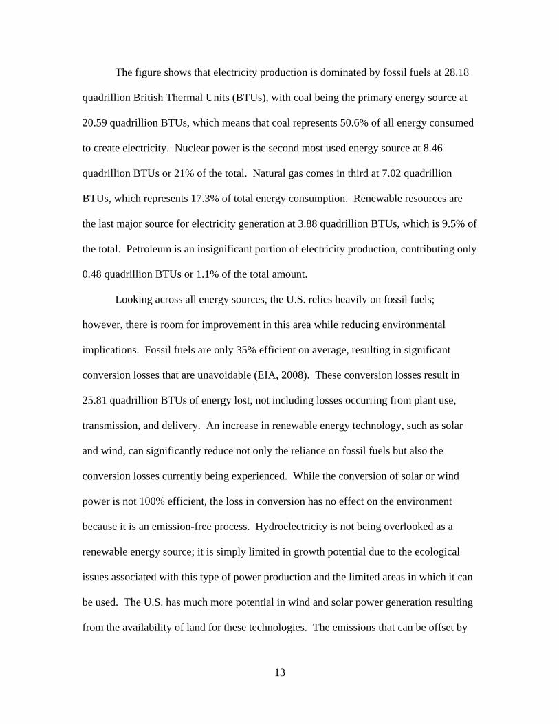
The figure shows that electricity production is dominated by fossil fuels at 28.18
quadrillion British Thermal Units (BTUs), with coal being the primary energy source at
20.59 quadrillion BTUs, which means that coal represents 50.6% of all energy consumed
to create electricity. Nuclear power is the second most used energy source at 8.46
quadrillion BTUs or 21% of the total. Natural gas comes in third at 7.02 quadrillion
BTUs, which represents 17.3% of total energy consumption. Renewable resources are
the last major source for electricity generation at 3.88 quadrillion BTUs, which is 9.5% of
the total. Petroleum is an insignificant portion of electricity production, contributing only
0.48 quadrillion BTUs or 1.1% of the total amount.
Looking across all energy sources, the U.S. relies heavily on fossil fuels;
however, there is room for improvement in this area while reducing environmental
implications. Fossil fuels are only 35% efficient on average, resulting in significant
conversion losses that are unavoidable (EIA, 2008). These conversion losses result in
25.81 quadrillion BTUs of energy lost, not including losses occurring from plant use,
transmission, and delivery. An increase in renewable energy technology, such as solar
and wind, can significantly reduce not only the reliance on fossil fuels but also the
conversion losses currently being experienced. While the conversion of solar or wind
power is not 100% efficient, the loss in conversion has no effect on the environment
because it is an emission-free process. Hydroelectricity is not being overlooked as a
renewable energy source; it is simply limited in growth potential due to the ecological
issues associated with this type of power production and the limited areas in which it can
be used. The U.S. has much more potential in wind and solar power generation resulting
from the availability of land for these technologies. The emissions that can be offset by

14
the use of renewable energy are huge; however, it is often difficult getting renewable
resources approved from an economic standpoint as their payback periods are not always
the most desirable.
Because power production plants lack the flexibility to change energy sources,
any fluctuation in the price of the natural resources required to produce electricity will
directly affect the end-user. Also, certain regions of the U.S. use different primary
energy sources for electricity production, creating a greater cost sensitivity towards the
dominant primary energy sources in that area. For example, an increase in the cost of
coal extraction would create a more significant end-user price increase in Pennsylvania
because of the higher percentage of coal-fired electricity production there compared to
Nevada which uses mostly hydroelectric power. These price concerns are typically of
much more concern to the end-user than are the environmental impacts.
Environmental Issues
Although energy use is necessary for our current standard of living and provides
many benefits, there are issues of environmental waste and pollution that need to be
addressed. This section will discuss some of the environmental issues caused by energy
use and describe a few of the harmful pollutants that exist in both power production and
street lighting. Light pollution associated with current street lighting designs will also be
discussed.

15
Greenhouse Gases
According to the Intergovernmental Panel on Climate Change (IPCC), greenhouse
gases (GHG) are “those gaseous constituents of the atmosphere, both natural and
anthropogenic, that absorb and emit radiation at specific wavelengths within the spectrum
of thermal infrared radiation emitted by the Earth’s surface, the atmosphere itself, and by
clouds” (IPCC, 2007). The IPCC recognizes gases such as carbon dioxide (CO2), nitrous
oxide (NO2), methane (CH4) and ozone (O3) as primary greenhouse gases. Greenhouse
gases are necessary for maintaining the earth’s temperature by trapping the heat from the
sun’s rays. The trapping of heat allows the earth to maintain a warmer temperature,
allowing ecosystems and life to survive. However, if the concentration of greenhouse
gases becomes too great, the earth’s temperature may begin to rise and thereby disrupt
current ecosystems. According to the National Oceanic and Atmospheric Administration
(NOAA) and the National Aeronautics and Space Administration (NASA), the earth's
average surface temperature has increased by about 1.2 to 1.4ºF in the last 100 years,
with the eight warmest years on record (since 1850) having occurred since 1998 (EPA,
2009). As shown in Figure 3, there has been an increase in anthropogenic activity over
the past 200 years, which scientists believe has attributed to the phenomenon known as
global climate change (EPA, 2009).

16
Figure 3. Anthropogenic Carbon Emissions 1800 - 2004 (Thorpe, 2008)
Mercury
Mercury (Hg) is “a naturally occurring element that is found in air, water and soil.
It exists in several forms: elemental or metallic mercury, inorganic mercury compounds,
and organic mercury compounds” (EPA, 2009). Mercury is an odorless, tasteless
substance that can be difficult to detect, so special care needs to be taken to minimize
exposure and contamination. Although it is a natural element found in the environment,
human activities such as mining and manufacturing have increased the amount of
mercury being distributed throughout the environment. The effects of mercury on
humans and the environment can be drastic. Mercury exposure at high levels can harm

17
the brain, heart, kidneys, lungs, and immune system of people of all ages, while high
level exposure to animals can cause death, reduced reproduction, slower growth and
development, and abnormal behavior (EPA, 2009). These effects vary depending on the
type of mercury present; however, all forms of mercury are considered toxic and should
therefore be handled and disposed of properly. In 1979, the U.S. Food and Drug
Administration (FDA) ruled that bottled water could contain no more than 2 parts per
billion (ppb) or about .000002 grams of mercury per liter of water for safe consumption
(Divison of Environmental and Occupational Health, 1998).
Light Pollution
Dust, water vapor, and other particles reflect and scatter light that is emitted into
the atmosphere, resulting in the sky glow found over most urban areas (Rea, 2000). Light
pollution is an unwanted consequence of outdoor lighting. Figure 4 illustrates various
types of light pollution and how they occur. Glare is a condition caused by stray light
scattered within the eye, which reduces the contrast of the retinal image (Rea, 2000).
Glare occurs when there is high contrast between the light and the environment or a non-
uniform distribution of luminance in the field of view. Direct glare is caused by light
aimed directly at the eye, whereas reflected glare is the result of light bouncing off of a
surface and toward the eye. Glare can be very distracting to drivers and can cause
temporary loss of vision as a result.
Light trespass occurs when light is unintentionally cast where it is not wanted
(Rensselaer Polytechnic Institute, 2007). Most cases of light trespass involve streetlights
that unintentionally illuminate windows and indoor areas of homes and businesses that

18
did not request it. This is usually caused by poor aiming of the light fixture or lack of
shielding on the light fixture itself. Sky glow is the illumination of the sky by both
natural and man-made lighting. Examples of naturally occurring sky glow come from the
moon, stars, and zodiacal light (Rensselaer Polytechnic Institute, 2007). Outdoor lighting
adds to sky glow when light is emitted directly upward by luminaires or reflected from
the ground, especially when moisture is present on the ground (Rensselaer Polytechnic
Institute, 2007). Sky glow makes it difficult for astronomers and others interested in
viewing the night sky to see stars and planets clearly. While sky glow may not have a
direct environmental effect, it shows that areas may be overlit, causing wasted light to
escape into the atmosphere.
Figure 4. General Lighting Issues Associated with Street Lighting (Rensselaer Polytechnic Institute, 2007)

19
Power Production
Most environmental waste associated with power production is in the form of air
pollutants, such as carbon dioxide (CO2), sulfur dioxide (SO2), and nitrogen oxides
(NOx). The Energy Information Administration (EIA) has tracked the amount of air
pollution associated with power production, as shown in Table 1. As the table shows, the
amounts of SO2 and NOX have steadily declined over the years, while the amount of CO2
has increased. This is of concern to most environmentalists, as CO2 is a major
contributor to global climate change.
Table 1. Emissions from Conventional Power Plants and Combined Heat-and-Power Plants (EIA, 2009)
Another air pollutant associated with power production is mercury. In 1999, the
EPA estimated that approximately 75 tons of mercury were found in the coal being
delivered to power plants each year and about two thirds of this mercury (50 tons) was
emitted into the air (EPA, 2009). Coal-burning power plants are thus the largest human
sources of mercury emissions in the United States, accounting for over 40 percent of all
domestic human-caused mercury emissions (EPA, 2009). These airborne mercury

20
emissions circulate around the environment and eventually settle on land and in
waterways, creating higher levels of mercury exposure than would normally be present.
The EPA has instituted regulations such as the Clean Air Mercury rule to reduce mercury
emissions and the environmental effects associated with power production.
Street Lighting
Energy is required for the production, use, and disposal of street lights, with the
bulk of the energy use being in the use phase. The amount of energy used by a street
light is directly related to the type and power rating of the street light. The higher the
amount of power consumed by street lighting, the more power that needs to be produced
by the power plants, which in turn produce the emissions discussed earlier. Electrodeless
induction and HPS street lighting technologies use mercury to aid in the lighting process.
Mercury is typically contained within the bulb during use; however, when the light bulbs
reach the end of their life, special care must be taken with disposal. The amount of
mercury contained within the bulbs can vary from 1mg to 15mg (Harder, 2007). As a
result, the EPA classified all hazardous waste lamps as universal waste in 40 CFR Part
273, requiring specialized disposal to minimize the opportunities for environmental
damage as a result from mercury contamination.
Light pollution is a major issue concerning street lighting. Issues such as glare,
light trespass, and sky glow have gotten the attention of many states. As a result, some
states have adopted legislation controlling light pollution, with other states pending
legislation (Rensselaer Polytechnic Institute, 2007). Figure 5 shows which states have
adopted or are pending statewide legislation. According to IESNA, the methods to best

21
control light pollution are to limit flux above the horizontal plane, minimize non-target
illumination, and turn off lighting during times of low use (Rea, 2000).
Figure 5. States adopting Light Pollution Legislation (Rensselaer Polytechnic Institute, 2007)
Environmental Policy
As a result of these and many other environmental issues, environmental policy
has become an important aspect of U.S. legislation. Since the 1970s, there have been
significant achievements in environmental regulation regarding air quality, water quality,
and hazardous waste. The Clean Air Act of 1970, which was amended in 1990, called for
air pollution prevention and reduction, emissions standards for all vehicles, acid rain
reduction, and ozone layer protection (EPA, 2009). President Bush also pushed for better
environmental stewardship through Executive Order 13423, calling for the use of
sustainable environmental practices through the acquisition of environmentally

22
preferable, energy-efficient products while reducing the quantity of toxic and hazardous
chemicals and materials acquired, used, or disposed of by the government (Bush, 2007).
Global climate change has also been a topic of concern and legislative debate as it
is most commonly associated with anthropogenic activity via carbon emission.
Discussion over this topic resulted in the creation of the Kyoto Protocol in 1997. The
Kyoto Protocol is an international agreement linked to the United Nations Framework
Convention on Climate Change (UNFCC) and designed to combat global climate change.
This environmental treaty attempts to “stabilize greenhouse gas concentrations in the
atmosphere at a level that would prevent dangerous anthropogenic interference with the
climate system” by setting binding targets for reducing greenhouse gas emissions in
industrialized countries (UNFCC, 2009). The protocol was initially adopted on 11
December 1997 in Kyoto, Japan, but was not entered into force until 16 February 2005.
As of December 2009, 187 countries have signed and ratified the Kyoto Protocol;
however, the United States is not one of them. The U.S. has signed the protocol but is
unwilling to ratify the treaty, with reasons ranging from lack of representation from
developing countries (CNN, 1997) to the exemption of China (Bush, 2001). Because the
U.S. has not ratified the Kyoto Protocol, they are not required to abide by it, which has
concerned advocates of global climate change.
In an effort to create awareness for global climate change, twelve states and
several U.S. cities, along with other activist groups, brought a lawsuit against the EPA in
an effort to force the agency to regulate carbon dioxide and other greenhouse gases as
pollutants in the court case Massachusetts vs. the EPA (Massachusetts vs Environmental
Protection Agency, 2007). In the case, the plaintiff claimed that global climate change

23
resulted in significant damage, creating land loss and endangering public health and
welfare. The Supreme Court directed the EPA to explain its position as to why carbon
emissions are not currently regulated. In a 5-4 ruling, the court decided that greenhouse
gases were air pollutants based upon the definitions stated in the Clean Air Act. The
ruling suggests that the EPA should regulate CO2 emission, but is not required to do so,
given the uncertainties surrounding global climate change.
The latest effort in environmental policy comes from the Lieberman-Warner
Climate Security Act of 2008. This bill would require the administrator of the EPA to
establish a federal greenhouse gas (GHG) registry for which companies must report fossil
fuel and GHG activity (U.S. Senate, 2009). The administrator would also need to
establish a GHG emission allowance transfer system (also known as cap and trade).
Under the cap and trade system, companies can produce emissions up to their allowance
without penalty; however, if more emissions production is required, those companies
must purchase excess emissions from companies who have produced fewer emissions
than they are allowed. While this legislation did not pass, it is clearly visible that steps
are being made to try and control GHG emissions on an industrial scale.
The U.S. government and other activist groups continue to work on solutions for
promoting environmentally friendly behaviors and practices. With a continued focus on
the reduction of greenhouse gas emissions and fossil fuel usage, while promoting an
increase in renewable energy sources, it is clear that the U.S. government is, at the very
least, considering the environmental effects associated with current energy consumption.
However, the government must also be careful of other consequences relating to these
emission measurements, such as the cost to the end-user. Instituting a cap and trade

24
program, or a carbon tax (paying a certain amount for each metric ton of carbon
produced), could have a significant cost impact on both businesses and end-consumers.
The Importance of Street Lighting
“The purposes of street illumination are: first to reveal, and second to embellish.
Protection against the hazard of criminal violence and collision; security in avoiding
obstacles and inequalities in roadway; facility in finding one’s way about, all require that
the light which is provided shall reveal what it is important to see on or about the street.
No system of street lighting is effective which fails to achieve this purpose” (Millar,
1924). In the Air Force, the primary purpose of outdoor lighting is to provide lighting for
exterior facilities, which require some degree of lighting during times of reduced
visibility for safety or for observation (Department of the Air Force, 1996). Aspects such
as security and safety are of significant importance to the government, especially for the
protection of military and intelligence assets (humans, equipment, information,
communication, and financial assets). “Darkness induces a sense of insecurity because it
cuts down visibility and recognition at a distance. Dark or dimly lit streets create a
limitless source of blind spots, shadows, and potential places of entrapment” (Painter,
1996). It is thus important that exterior lighting be improved, as “improved lighting is an
immediate means of cost effectively creating a sense of public safety, enhancing the
quality of the built environment and increasing the number of people on the streets after
dark” (Painter, 1996). Painter and Farrington (2001) show the cost-benefit of improved
street lighting based on crime reduction. The study found that for crimes such as
burglary, vandalism, vehicle crime, cycle theft, rob/snatch, assault, and threat/pest, there

25
was a significant decrease in crime after improved lighting had been introduced, resulting
in a savings of £558,415 over the course of one year (Painter & Farrington, 2001).
While the elimination of blind spots and dark spots is important when evaluating
street lights, there are also other factors that contribute to the effectiveness of street
lighting. “Effectiveness in a street lighting system, like personal charm, is recognized
when encountered, but it is difficult to define. The effectiveness of the lighting system
depends upon the right combination of several qualities, some of which are perhaps
intangible” (Millar, 1924). Factors such as location of the lamps, mounting height,
characteristics of lighting, and illumination affect the ability of street lamps to perform
effectively and efficiently. With the importance of street lighting defined, the next
section describes some of lighting characteristics that need to be understood when
comparing lighting technologies.
Lighting Characteristics
Before lighting technologies can be compared, a few terms regarding lighting
characteristics need to be defined in order for the comparisons to make sense. The Color
Rendering Index (CRI) is understood to be a measure of how well light sources render
the colors of objects, materials, and skin tones. The CRI is measured by comparing the
appearance of eight color samples under the light in question and a reference light source.
The average measured differences are subtracted from 100 to get the CRI (EERE, 2008).
A CRI of 100 suggests that the colors rendered under that particular light source are the
same as the color rendering properties of daylight. The CRI is a good measure for
showing how well colors are perceived by the human eye, which can help with the

26
identification of objects under artificial light. Having a lighting system with a high CRI
is useful in areas that require faster reaction times or better recognition of objects and
people, such as security checkpoints. Color temperature is a description of the color
reproduced by the light source, typically classified in degrees Kelvin (K). Lights with
color temperatures above 5000K have a blue-white color, while lights with a color
temperature below 3000K are more yellowish-red in appearance.
Efficacy refers to the amount of light produced by a light source as a ratio to the
power needed to produce that light (EERE, 2009). This term is typically defined as
lumens per watt. This is different from illuminance, which is the total amount of light
over a given area and is typically expressed in foot-candles or lux (lumens per square
meter). Vertical illuminance is the amount of light density measured on a vertical plane,
while horizontal illuminance is the amount of light density measured on the horizontal
plane.
Types of Street Lighting
This section will discuss both current and emergent technologies in the street
lighting industry. The history of each lighting application will be explained, along with
its construction, how it works, and its perceived benefits and drawbacks.
High Pressure Sodium
High pressure sodium lamps have been around since the 1970s. They are
considered part of the high-intensity discharge (HID) family of lights. This means that
the lamp produces light by using an electrical arc discharge contained inside an arc tube
inside a bulb. The arc tubes typically contain tungsten electrodes that terminate the arc

27
discharge at each end of the arc tube. There are typically starting gases (e.g., neon,
xenon, argon) inside the arc tube that ionize easily at low pressure and normal ambient
temperatures. The arc tube is contained inside a glass outer bulb built to protect the arc
tube and internal electrical connections from the elements. The outer glass bulb can be
coated with a diffusing material to reduce or increase the source brightness of the lamp.
The gas in between the inner and outer bulb is typically a low pressure gas or vacuum.
These lamps are known for emitting UV energy that is typically captured by the outer
bulb; however, if the outer bulb were to break, the UV energy emitted can produce skin
reddening or eye damage (Rea, 2000).
Light in a HPS bulb is produced by electric current passing through sodium vapor.
The arc tubes are made out of polycrystalline alumina to prevent sodium attack at high
temperatures. The arc tube also contains both xenon as a starting gas and a small
quantity of sodium-mercury amalgam, which is in liquid form at startup and partially
vaporized as the bulb reaches operating temperature. The mercury acts as a buffer gas to
raise the gas pressure and operating voltage of the lamp. The amount of mercury in the
bulb varies depending on the rated power of the bulb and can range from 0 to 50mg
depending on manufacturer and type (Keith, 2003) with an average of 15mg being the
standard for 250-watt bulbs (Harder, 2007). The outer glass prevents chemical attack of
the electrodes and also maintains arc tube temperature by isolating the metal from
ambient temperature effects. These lamps can operate in any position or orientation
without any significant effects on light output. A picture of a HPS bulb detailing its
construction can be seen in Figure 6.

28
Figure 6. High-Pressure Sodium Bulb Components (Rea, 2000)
High-pressure sodium lamps radiate light across the visible spectrum. Their
ability to transmit light depends on the internal pressurization of the bulb. The higher the
sodium pressure, the higher the color temperature and color rendering index; however,
bulb life is shortened as a result. White high-pressure sodium lamps have been
developed with color temperatures between 2700K and 2800K and a CRI between 20 and
70. The efficacy of HPS ranges between 45 and 150 lumens per watt depending on the
lamp wattage and desired CRI. Rated lamp life is typically defined as the time after
which 50% of a large group of lamps are still in operation. The life of an HPS lamp is
limited by a slow rise in operating voltage that occurs over the life of the lamp due to the
buildup of impurities on the electrodes. One sign of HPS reaching the end of its life is a
constant “cycling,” where the lamp turns itself on and off because it can no longer
29
maintain the voltage needed for proper operation. The typical rated life for an HPS bulb
is between 12,000 and 24,000 hours (approximately 3-6 years).
An HPS fixture is typically made up of 3 parts: the bulb, the ballast, and the
fixture. Figure 7 shows the basic workings of this type of lighting system. Because of
the size of HPS bulbs, no starting electrode is included in the bulb. Also, HID lamps
have negative volt-ampere characteristics which create a requirement for a current-
limiting device, usually in the form of a ballast or transformer, to be provided to prevent
excessive lamp and line currents necessary for stable operation. For these lamps to turn
on, a high-voltage, high-frequency pulse must be provided by an ignitor (typically built
into the ballast) to excite the starting gas in the tube. As the gases warm up, the amalgam
is slowly vaporized while the voltage continues to rise until the light has reached its
operating temperature, changing color and lighting intensity as it arrives to this point.
This process can take up to 10 minutes on initial startup. Restrike times are typically less
than a minute with the bulb taking 3 to 4 minutes to warm up (Rea, 2000).
Advantages
When compared with other HID lighting technologies, such as metal halide (MH),
HPS offers significant advantages. HPS lighting has a longer bulb life, averaging
between 12,000 to 24,000 hours versus 10,000 to 15,000 hours for MH bulbs (Harder,
2007). HPS also produces approximately 42 percent more lumens per watt (W) while
reducing sky glow. HPS lights are very good at providing adequate light because they
are available in power ranges from 100W all the way up to 1000W for special
applications.

30
Figure 7. High Pressure Sodium Construction (Wikipedia, 2009)
Disadvantages
HPS lighting is most notable for its orange glow, which does not render colors
very well, hence a lower CRI. HPS lights also require very high initial input power to
start the arc in the bulb, resulting in significant energy use. At the end of their life, HPS
bulbs begin to flicker and cycle, causing inconsistent light output. HPS fixtures, while
designed to meet IESNA lighting standard distribution types, cause significant light
pollution due to their use of a drop lens to project light from the fixture.
High Pressure Sodium Lighting Summary
HPS lighting is the lighting of choice for most cities, municipalities, and military
installations (Department of the Air Force, 1996). While they may require constant
maintenance and require high amounts of power to operate, they are reliable under most
weather and temperature conditions. They are about 50% efficient when converting

31
energy into light, and they are also readily available. The technology has been around for
quite some time and most people have grown accustomed to the orange glow they emit.
Electrodeless Induction
Although electrodeless lamps are a relatively new lighting technology for street
lighting, the principles behind the technology date to the 1890s when Nikolas Tesla
demonstrated the transfer of power to electrodeless incandescent and fluorescent bulbs
(Roberts, 2009). Tesla was granted patent 454,622 to cover an early form of induction
lamp. Electrodeless lighting is a special form of fluorescent lighting in which an
electromagnetic (EM) field, instead of an electric current through electrodes, is used to
excite the gas in a bulb. There are two types of electrodeless bulbs according to how they
produce EM fields. These categories are inductive discharge and microwave discharge.
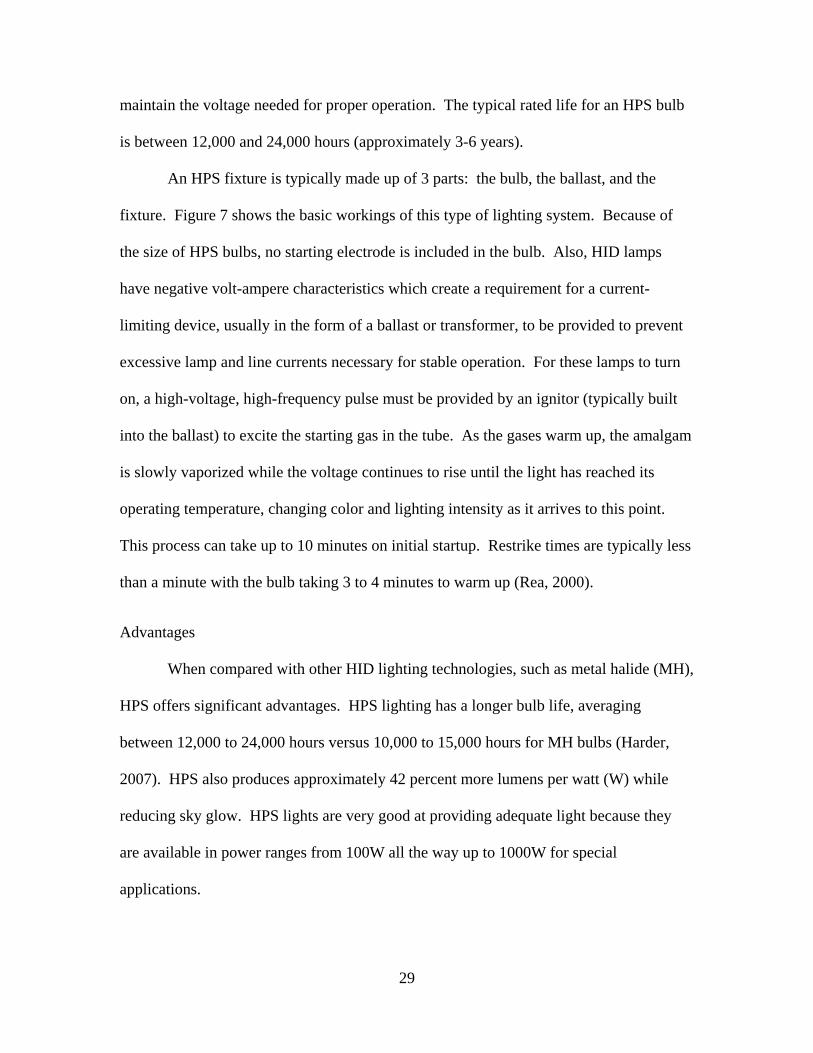
Induction lamps operate using the same principles as conventional fluorescent
lamps, which is through the excitement of phosphors found in those lamps. Figure 8
shows a diagram of an induction lamp. The operation of the lamp operates in the
following manner (in coordination with the numbers in Figure 8) (Rea, 2000).
1. The radio frequency power supply sends an electric current to an induction coil (a wire wrapped around a plastic or metal core).
2. The current passing through the induction coil generates an EM field.
3. The EM field excites the mercury in the gas fill, causing the mercury to emit ultraviolet (UV) energy.
4. The UV energy strikes and excites the phosphor coating on the inside of the glass
bulb, producing light.
32
Figure 8. Induction Light (Rea, 2000)
Advantages
Because induction lamps do not require electrodes, higher efficiency gases can be
used that would normally deteriorate the electrodes. These gases assist the induction bulb
to last longer, anywhere from 65,000 up to 100,000 hours (Roberts, 2009; Cornerstone
Energy Solutions Inc., 2009). These special gases also help increase the efficacy of the
fixtures, ranging anywhere from 40 to 87 lumens per watt (Cornerstone Energy Solutions
Inc., 2009). The correlated color temperatures for induction are in the range of 2700K to
4000K and their CRI is typically greater than 80 (Lai & Lai, 2004). Induction lamps are
also an “instant on” technology, meaning that they light instantaneously with restrike
times under 1 second. These lamps can also perform hot restrikes, meaning the bulb does
not need to cool before the light can cycle back on, unlike HID technologies.

33
Disadvantages
One of the main disadvantages of induction lighting is the upfront cost. They are
2 to 5 times more expensive than a standard HPS fixture. Another disadvantage is the
mercury present in the fixture. While induction lamps contain only 5mg of mercury,
which is less than HPS, it is still a hazardous substance that requires special attention
when being disposed of. Another disadvantage is the fragility of the bulb due to its glass
construction. There have also been some claims that the frequency generators have had
issues with 480V lines. Induction lamps also require the use of drop lenses to increase
their effectiveness, which helps them contribute to various forms of light pollution
(Cornerstone Energy Solutions Inc., 2009).
Electrodeless Induction Lighting Summary
While induction lamps have a higher upfront cost when compared to other
lighting technologies, their equipment service life and low maintenance intervals make
them very attractive for long-term projects. These bulbs operate similarly to the HPS
technology, allowing adopters upgrading from HPS fixtures to be more easily familiar
with their operation and components.
Light-Emitting Diode
Light-emitting diodes (LEDs) are the latest technology to appear in the street
lighting industry. A light-emitting diode is an electronic component that allows current
to flow in one direction and create light as the current passes, given a set threshold
voltage is met. The LED is a chip made up of two semiconductor materials layered on a
substrate injected with impurities to create a p-n junction. Figure 9 displays a p-n

34
junction and how the electrons move between that junction inside the LED. Current
flows easily from the p-type side, known as the anode, to the n-type side, known as the
cathode; however, current cannot easily flow in the other direction. When electrons meet
holes in the junction, energy is released as a photon. The color of the light emitted
depends on the band gap energy of the materials that form the junction.
Figure 9. P-N Junction of a Light-Emitting Diode (Wikipedia, 2009)
Unlike most other lighting technologies, LEDs emit light by electronic excitation
(electroluminescence) rather than heat generation (incandescence). The LED was
invented in the 1920s by Russian Oleg Losev; however, it was not until 1962 when the
first practical visible-spectrum LED was invented at General Electric’s Advanced
Semiconductor Laboratory (Navigant Consulting Inc., Radcliffe Advisors Inc., and SSLS
Inc., 2009). The first LEDs were red in color, but over time green and blue LEDs were
created using different material compounds. In order for LEDs to appear white, either a

35
combination of the red, green, and blue LEDs should be made or a yellow phosphor
coating can be placed on a blue LED. Figure 10 shows how these two processes work to
produce white light.
Figure 10. Methods for Making White LEDs
The LED was originally used as an indicator light for items such as radios and
computers. The creation of white LEDs has paved the way for them to be used in
numerous applications, such as televisions, cellular phones, and automotive lighting.
LED fixtures for street and parking lot lighting package a number of LED chips onto a
coated printed circuit board and enclose them in a housing suitable for the outdoor
environment. The LED fixture requires no ballast or capacitors like the other lighting
technologies; however, it does require a power supply to convert alternating current (AC)
line voltage into low voltage direct current (DC). The power supply can either be housed
in the enclosure or mounted on the printed circuit board along with the LEDs (San Diego
Regional Energy Office, 2003).
Advantages
Unlike conventional HID lighting, an LED is not a one-bulb fixture. An LED
fixture contains many smaller LEDs, classifying this technology as a point-source

36
technology. Because the individual LEDs in the fixture can be directed toward a specific
location, this allows flexibility in the design and greater optical control. Conventional
HID fixture optical losses range from 40% to 50%, meaning that only half of the source
light is directed in the desired direction. LEDs fixtures can be 80 to 90% efficient in their
light transmission, allowing them to use less power to transmit the same amount of light
(San Diego Regional Energy Office, 2003). LED lighting fixtures can also be designed
to reduce backlight and uplight while increasing the uniformity of light distribution
across the target area. Better surface illuminance uniformity and higher levels of vertical
illuminance are possible with LEDs and close-coupled optics compared to HID
luminaires (EERE, 2008)
LEDs are also a solid-state technology, giving them increased durability and
ruggedness against the elements. Because there are no moving parts or gases in the light
itself, it is capable of avoiding premature failure due to direct impact or moisture
(Cornerstone Energy Solutions Inc., 2009). LEDs require low direct current voltage and
low power to operate, which results in reduced energy use. Depending on the
application, they can demonstrate anywhere from 50% to 90% in energy savings (San
Diego Regional Energy Office, 2003). Their usable life ranges anywhere from 50,000 to
100,000 hours, depending on input current and thermal design (San Diego Regional
Energy Office, 2003). The usable life of an LED fixture is determined to be when the
light output of the fixture falls below 70% of its initial lumen output (Rea, 2000).

37
Disadvantages
Although LEDs have many advantages, there are a few significant disadvantages.
Because of the construction of LEDs, they are very susceptible to high p-n junction
temperatures, causing premature failure of the device if it gets too hot. Because most
outdoor LED luminaires are high-power devices (>350 milliamperes), it is especially
important to keep both junction temperatures and ambient fixture temperatures low to
ensure that light production is not significantly affected. Most LED specifications show
performance at an ambient temperature of 25°C; however, higher temperatures can
significantly affect the relative flux of the colors used in LED lighting, as shown in
Figure 11. To keep temperatures down, heat sinks and other cooling technologies need to
be properly designed and applied in order to keep the LED luminaires from overheating.
Another issue concerning LEDs is maintaining the consistency of white light.
The two methods shown in Figure 10 each have their flaws. The pc-LED has issues due
to natural variations in LED wavelength or in the phosphors themselves. The light is also
then susceptible to variations in LED optical power, peak emission wavelength,
temperature, and optical characteristics (Navigant Consulting Inc. et al, 2009). The
phosphors applied to the LED also lower its efficiency. When using color-mixing LEDs,
there can be issues with the blending of the colors, especially with the green LEDs due to
the absence of efficient emitters. This can significantly limit efficacy. There is also
increased complexity when blending the colors, potentially requiring multi-die mounting
and sophisticated optics. Color control feedback circuitry to address the different
degradation and thermal characteristics may also be required (Navigant Consulting Inc. et
al, 2009). Issues with power supplies, heat, and lightning protection have made

38
consumers leery of their ability to hold up to the elements. Additionally, because LEDs
are an electroluminescent light source with a significantly different luminaire
construction compared to HPS and induction, current lighting regulations and testing
practices are unable to properly test the LED technology.
Figure 11. Relative Flux Vs LED Die Junction Temperature (Cooper, 2007)
Special Considerations
The steady improvement of LEDs makes them a very attractive technology. As
Figure 12 shows, LEDs have the best growth potential out of all the lighting technologies
currently on the market. Figure 13 illustrates the difference between the price and lumen
output of LEDs since 1965 with projections pertaining to lumen efficiency out to year
2020; this shows the rapid pace of improvement for LED technology.
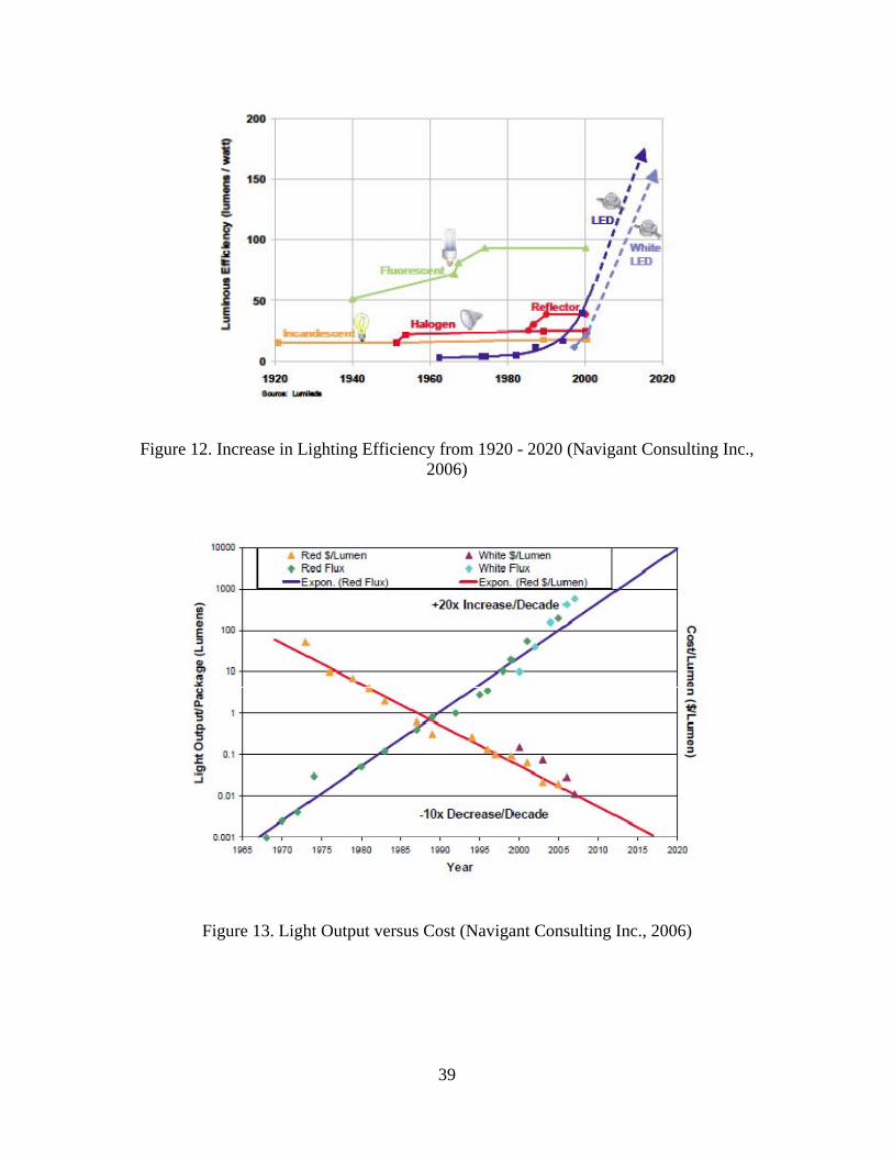
39
Figure 12. Increase in Lighting Efficiency from 1920 - 2020 (Navigant Consulting Inc., 2006)
Figure 13. Light Output versus Cost (Navigant Consulting Inc., 2006)
40
Light-Emitting Diode Lighting Summary
Solid-state lighting (SSL) is the newest technology on the market right now. With
more than $37 million being spent on the research, development, and manufacturing by
the Department of Energy (DOE), SSL certainly seems to be the technology of the future
(EERE News, 2010). Although SSL lighting has great potential, LEDs have been mostly
used on a trial basis because the technology has yet to prove itself.
Lighting Regulations and Standards
While the illumination of streets is a standard practice across the United States
and many other countries around the world, lighting standards and regulations vary. In
the United States, most areas follow IESNA standards in conjunction with other
organizations such as the American National Standards Institute (ANSI), Underwriters
Laboratories (UL), the National Electrical Manufacturers Association (NEMA), and the
National Institute of Standards and Technology (NIST). While these standards have been
developed by experts, the end user determines whether a deviation from these lighting
standards is required. For instance, the Air Force has developed its own set of standards.
All Air Force installations are required to abide by Unified Facilities Criteria
(UFC) 3-530-01, Design: Interior and Exterior Lighting and Controls. This UFC is the
main document applicable to both indoor and outdoor lighting. While this UFC refers
extensively to the IESNA handbook, there are areas where the UFC supersedes the
standards specified in the handbook. This UFC defines the critical design criteria for
exterior lighting associated with parking lots and roadways as direct glare, light pollution,
reflected glare, vertical illuminance, small target visibility, and target horizontal

41
illuminance (Department of the Air Force, 2006). Some of these design criteria have
already been discussed in earlier sections. The other design criteria will be explained
below along with the three methods for testing the effectiveness of street lighting systems
and fixtures.
Illuminance is the simplest method for determining lighting needs. This method
simply measures the amount of light produced on a given surface and measures it in foot-
candles or lux. Tables 2 and 3 show the recommended amounts of illuminance based on
the type of pavement (Table 2) and traffic (Table 3) present for each area. The problem
with this method is that it only looks at incident light and does not take into account the
light reflected off of the surface. This method is not recommended according to UFC 3-
530-01 because it usually produces poor small target visibility results, which can have a
significant impact on peripheral vision and object recognition.
The luminance method simulates driver visibility by assessing the quantity and
quality of light reflected by the pavement surface to the motorist’s eye from contributing
luminaires (Bureau of Design and Environment Manual, 2002). Although more complex,
this method accounts for glare potential and other indirect lighting circumstances, thereby
creating a better sense of how well a certain lighting system design will perform. This
method is recommended as an excellent alternative to illuminance as it provides a more
“real world” experience. The small target visibility (STV) method is similar to the
luminance method but with an additional test for identifying targets across the ground.
This collective visibility of the targets is calculated and expressed as a weighted average.
This method is preferred because it has a high emphasis on security and peripheral vision
(Department of the Air Force, 2006).

42
Table 2. IESNA RP-8-00 Recommended Illuminance for Intersections (Rea, 2000)
Table 3. IESNA RP-8-00 Guidance for Roadway and Pedestrian/Area Classification for Determining Intersection Illumination Levels (Rea, 2000)

43
Special Criteria for LED Fixtures
Because LEDs are such a radical departure from standard lighting technologies,
separate standards have been and are being developed. Some of the currently available
standards are ANSI C78.377-2008: Specifications for the Chromaticity of Solid-State
Lighting Products, IES LM-79-2008: Approved Method for the Electrical and
Photometric Testing of Solid State Lighting Devices, IES LM-80-2008: Approved Method
for Measuring Lumen Depreciation of LED Light Sources, and IES RP-16: Addendum a,
Nomenclature and Definitions for Illuminating Engineering. Other standards are also in
development, such as NEMA SSL-1: Driver Performance Standard, NEMA LSD-49:
Solid-State Lighting – Best Practices for Dimming, UL 8750, LED Safety, TM-21,
Method for Estimation of LED Life, and LM-XX1, Approved Method for the
Measurement of High Power LEDs. UFC 3-530-01 does not currently permit the
installation of LED luminaires for parking lot and roadway lighting; however, LED
technology is allowed for use as interior exit signage. The Air Force is creating
Engineering Technical Letter (ETL) 10-02 that plans to address LED fixture design and
installation criteria for exterior lighting applications.
Lighting Case Studies
With the emergence of induction and LED technologies in street lighting, there
have been a multitude of pilot studies performed in different areas, using collaborations
between local utilities, federal agencies, lighting manufacturers, and power companies.
These studies test whether LED and/or electrodeless induction technologies truly offer an
advantage over the HPS and metal halide fixtures currently in use. Energy savings and
upfront costs were used in most studies to determine the economic feasibility of

44
switching technologies. Only one of these studies looked at the environmental impact
associated with differing lighting technologies.
San Diego LED Assessment
In August 2003, Tetra Tech EM, Inc., prepared a study for the San Diego
Regional Energy Office (SDREO) that performed a technology assessment for LED
street and parking lot lighting applications. The study was conducted under the
SDREO’s Public Agency Energy Partnership Program in partnership with the City of
Chula Vista. The applicability, commercial availability, energy savings, and cost were
assessed using data provided by product manufacturers, interviews with manufacturers
and the users’ community, and other reports and information from the lighting industry.
Qualitative data were generated during field inspections of Chula Vista’s street and
parking lot lights and the limited number of LED parking lot lights.
The study compared and contrasted LED fixtures from three different companies.
Fluorescent lighting technology using T-5 fluorescent lights was also mentioned in the
study as another alternative, but the main focus of the study was on LED lighting.
Factors such as luminaire power, lumen output, efficacy, operating temperature,
warranty, and cost were included in the study, although only manufacturer’s data was
used in the analysis, no actual measurement. The study also performed a utility rate
analysis. Because the street lights are not metered, the annual cost for each lighting
fixture was estimated. An economic assessment was performed comparing a 100W HPS
fixture to the different LED fixtures using estimated energy savings and maintenance cost

45
savings based on the manufacturer data they were given. The results are outlined in
Table 4.
Table 4. LED vs. HPS Power Usage and Energy Savings (San Diego Regional Energy Office, 2003)
These results show that the LED fixtures were between 58% and 81% more
efficient than HPS fixtures. The simple payback period ranged from 9.2 to 20.1 years for
the various LED products when replacing a 100W HPS fixture; it ranged from 6.7 to 14.3
years when 150W HPS fixtures were replaced. A comparison was also made using a
53W T-5 fluorescent lighting fixture. The estimated energy savings were approximately
59%, with an annual $41 energy cost savings when compared with a 100W HPS lamp.
The simple payback was estimated at 4.9 years, suggesting that at the time of the study,
fluorescent lighting would be more cost effective than using LED lighting. This
conclusion was attributed to the high initial costs associated with LED technology and
suggests that continued price reductions would make LED lighting more cost competitive
with other technologies.

46
Oakland LED Assessment
A demonstration assessment of LEDs was performed in Oakland, CA, in
November 2008 by the DOE and Pacific Gas & Electric (DOE and PG&E, 2008) as a
follow-up to a previous street lighting assessment (Phase II report) that compared LED
luminaires to a base case of HPS luminaires. The study replaced some of the LED
luminaires used in the Phase II study with newer LED luminaires by the same
manufacturer. The performance of all three alternatives (HPS, LED Phase II, LED Phase
III) was then compared based on lighting performance, electrical power measurements,
and economic analysis. The Phase III LED luminaires drew approximately 58W, 20
watts less than the Phase II LED luminaires and 63W less than the HPS luminaires.
The results of the electrical measurements can be seen in Table 5. These savings
were calculated using an estimated 4,100 annual hours of operation. Despite the decrease
in average power for the Phase III luminaires, they provided illumination roughly
equivalent to the Phase II LED luminaires and were sufficient to meet the City of
Oakland’s requirements in all but the largest pole spacing scenarios. They were also
similar in minimum illuminance and maximum-to-minimum uniformity ratios. The
simple payback period for the Phase III luminaires ranged from 5 to 14 years, depending
on the maintenance and replacement scenario, where the range was 12 to 24 years for the
Phase II luminaires under the same maintenance and replacement scenarios. In essence,
the study showed that LED technology continues to improve at a rapid pace, making it
more economically justifiable, as was suggested by the SDREO study 5 years earlier.

47
Table 5. Phase II and III Power and Energy Savings (DOE and PG&E, 2008)
DOE CALiPER Program
The DOE Commercially Available LED Product Evaluation and Reporting
(CALiPER) program supports the testing of a wide array of Solid State Lighting (SSL)
products available for general illumination. This program independently tests and
provides unbiased information on the performance of commercially available SSL
products. The results from CALiPER tests provide guidance for DOE planning for SSL
research and development, support DOE GATEWAY demonstrations (under which the
Oakland study is classified), product performance information, and guide the
development of standardized test procedures and measurements (Department of Energy,
2009). All luminaires are tested by one of several prequalified lighting testing
laboratories that assist the program. The tests check lighting performance, thermal
performance, and electrical power measurement.
The CALiPER test involved the measurement of five LED street lights, two
induction street lights, and one HPS street light as a benchmark. This test was conducted
from September 2008 to January 2009. Table 6 displays the summarized testing results,
showing that SSL street lights can vary significantly in power consumption, efficacy,
lumen output, and color temperature. Power factor and CRI are pretty consistent

48
throughout the range. HPS technology shows a lower CRI with significantly higher
lumen output at significantly higher power consumption. The efficacy for HPS was
above the SSL average for this test, while power factor was significantly lower than all
the other technologies involved. The induction street lights showed a higher CRI and
lumen output compared to the average SSL street light, while its power consumption and
power factor were close to the averages of the SSL. It should be noted that the induction
lamps were highly sensitive to thermal conditions, which resulted in the ranges shown.
This test proves that not all LED street lamps are alike and that testing should be an
integral step of any procurement process.
Table 6. DOE CALiPER Study Results (DOE, 2009)

49
Groton Induction Study
Morante (2008) conducted a study for Groton Utilities in Groton, CT, testing the
theory that tuning lower power lights to the mesopic (combination of photopic and
scotopic vision in low light) needs of drivers and pedestrians would make a noticeable
improvement. For the study, 100W HPS fixtures were replaced with 55W induction
fixtures and ceramic metal halide fixtures. A survey was handed out to collect
perceptions of the lighting change. An economic analysis was also performed to
determine if either technology could cost effectively replace the existing HPS lighting.
The study found that drivers and pedestrians perceived they could see better and felt safer
with light sources tuned toward the needs of mesopic vision. The economic analyses
showed a simple payback for the induction lamp of 7.1 years for new installations and
13.9 years when retrofitting an existing HPS installation. Energy efficiency and power
data were estimated using manufacturer data for the economic analysis.
Life-cycle Comparison: Compact Fluorescent and Incandescent Bulbs
So far, all of the studies mentioned have only addressed the financial and energy
savings associated with the use of different lighting technologies without mentioning any
of the environmental impacts that may result from the change in technology. Soneji
(2008) compared the life-cycle energy usage between compact fluorescent (CFL) and
incandescent light bulbs. The study used the Process-Sum and Economic Input-Output
Life-cycle Assessment (EIO-LCA) methods. The results of the study found that although
manufacturing energy use for CFLs was higher, lower energy consumption in the use
phase provides a significant savings over incandescent light bulbs over the life-cycle.

50
The study also noted that mercury use in CFLs (5mg per bulb) is offset by the reduction
in power usage compared to incandescent lighting. While this study did not compare
outdoor lighting technologies, it does show how EIO-LCA can be used to measure the
environmental impacts associated with the use of different lighting technologies.
Summary
With an understanding of the policy, regulations, and technologies surrounding
street lighting, it is clear that additional studies are necessary to determine the long-term
feasibility and practicality for implementing new street lighting technologies from both
an economic and environmental perspective. The case studies discussed substantiate the
use of both life-cycle cost analysis and economic input-output life cycle assessment
methodologies, as these tools were used successfully in their respective studies to show
both the economic and environmental effects associated with different lighting
technologies.
The next chapter will cover the methodologies used in this study. It builds on the
studies mentioned in this chapter and addresses how both the economic and
environmental aspects of the study were handled. It also shows how both methodologies
were used together to create an understanding of the primary and secondary effects
associated with the life-cycle process of street lighting.
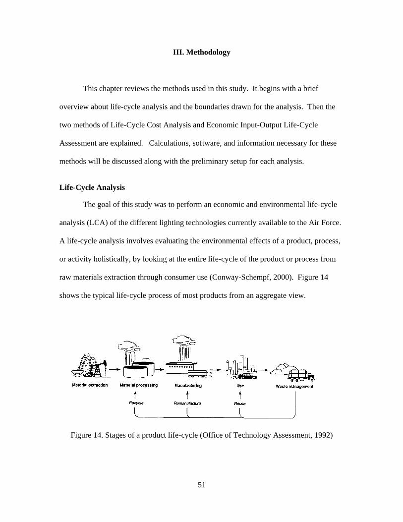
51
III. Methodology
This chapter reviews the methods used in this study. It begins with a brief
overview about life-cycle analysis and the boundaries drawn for the analysis. Then the
two methods of Life-Cycle Cost Analysis and Economic Input-Output Life-Cycle
Assessment are explained. Calculations, software, and information necessary for these
methods will be discussed along with the preliminary setup for each analysis.
Life-Cycle Analysis
The goal of this study was to perform an economic and environmental life-cycle
analysis (LCA) of the different lighting technologies currently available to the Air Force.
A life-cycle analysis involves evaluating the environmental effects of a product, process,
or activity holistically, by looking at the entire life-cycle of the product or process from
raw materials extraction through consumer use (Conway-Schempf, 2000). Figure 14
shows the typical life-cycle process of most products from an aggregate view.
Figure 14. Stages of a product life-cycle (Office of Technology Assessment, 1992)

52
The product life-cycle typically has five stages. The first stage involves
extracting raw materials from the natural earth, such as iron ore, oil, wood, sand, and
water. The next stage is processing those raw materials into finished materials, such as
oil into plastic and iron ore into steel. The third stage is to turn those materials into a
final product. This stage encompasses both turning materials into parts and assembling
those parts into a final product. The fourth stage is the use stage, where the product is
used for its intended purpose. The final stage is the disposal or end-of-life stage, where
the product is discarded to a landfill or recycled for reuse. Street lighting fixtures have a
similar life-cycle process, which enables the use of LCA as a feasible process by which to
analyze the data. This study used two different types of LCA to create the holistic picture
necessary for a true understanding of the economic and environmental impacts associated
with the different lighting technologies. For this study, the economic life-cycle analysis
will focus only on the use phase, while the environmental life-cycle analysis will
concentrate on the manufacturing, use, and waste management phases of the product life-
cycle.
Life-Cycle Cost Analysis
The National Energy Conservation Policy Act (42 U.S.C. 8254) established the
protocol for all federal agencies to use life-cycle cost methods and procedures for
investment evaluations. Practical and effective present value (PV) methods should be
used for estimating and comparing life-cycle costs for federal buildings, using the sum of
all capital and operating expenses associated with the energy system of the building
involved over the expected life of such system or during a period of 40 years, whichever

53
is shorter, and using average fuel costs and the current discount rate (42 USC 8254,
1978). In response to this act, the Federal Energy Management Program (FEMP) under
the DOE partnered with the National Institute of Standards and Technology (NIST) to
create the Life-Cycle Cost Analysis (LCCA) model, which is an economic method of
project evaluation in which all costs arising from owning, operating, maintaining, and
ultimately disposing of a project are considered to be potentially important to that
decision (Fuller & Petersen, 1996). This model includes the calculation and comparison
of facility energy projects by tracking the savings-to-investment ratio (SIR), adjusted
internal rate of return (AIRR), simple payback period (SPP), and discounted payback
period (DPP). The combination of these measures facilitates the direct comparison of
two or more projects to determine which project is the most cost-effective solution.
While this method was originally designed for measuring the differences in
energy use and long-term costs between different projects relating to a building, it can
easily be applied to street lighting alternatives since the criteria used to evaluate street
lights is virtually the same as those criteria needed for evaluating other facility-related
energy projects. To reduce errors in calculation and streamline the use of LCCA, FEMP
and NIST created the Building Life-Cycle Cost 5 (BLCC5) software. It is currently the
only software recommended for use by the Air Force in calculating life-cycle costing
associated with energy projects and is required under 10 CFR 436 subpart A.

54
Requirements for BLCC5
The BLCC5 software requires some assumptions about design life, installation
and acquisition costs, energy use, and maintenance costs of each lighting technology.
Therefore, the following assumptions were the basis for this analysis and were the values
input into the BLCC5 software.
Design Life
To ensure this study accurately depicted a real-world scenario, a design life for
the lighting technology was based on the long-term effects of using the lighting
technologies during their use phase. The design life consisted of both an equipment
service life and comprehensive design life. The comprehensive design life and
equipment service life was used to calculate the life-cycle cost using BLCC5 software.
Equipment Design Life
An important aspect of LCA is the estimated design life of the equipment being
used. The equipment design life was determined by the average service life between
manufacturers of the same lighting technology. This eliminates any low or high design
life estimates associated with a certain technology that could skew the analysis, as most
manufacturers claim different design lives for their products based on their design goals.
The estimated service lives for each technology are listed in Table 7.
Table 7. Equipment Service Life before Bulb or Fixture Replacement
Lighting Technology Service Life
HPS 17,000
LED 50,000
Induction 88,000

55
The Illuminating Engineering Society of North America (IESNA) recommends
standards for all types of lighting. The service life for a light is determined by the length
of time the light is expected to last until it is no longer bright enough to provide sufficient
illumination. In the case of HPS and electrodeless induction, the fixture has reached the
end of its service life when it is estimated that half of the fixtures of that type will fail.
LED standards are slightly different due to the difference in technology. LED fixtures
are deemed to have reached the end of their service life when they have reached 70% of
their initial lumen output. Given these service lives, the study assumed the fixtures
would last to their service lives with no additional maintenance or replacement necessary.
Comprehensive Design Life
For this study, a comprehensive design life of 20 years was chosen. Although
design lives of 25 years are mandated through Executive Order 13123, the continued
advancements in lighting technology would render the findings of this study obsolete. A
25-year study period would also create a need to calculate salvage values for the newer
technologies, as they would still have a significant service life associated with them. The
20-year study period allows for all the technologies to be used for their respective
minimum service lives, providing a more realistic picture of the long-term costs and
benefits associated with street lighting. Making the study any shorter would deprive
future savings associated with any of these technologies. Lengthening the study period
would be unrealistic as newer, more efficient technologies are likely to exist in the future,
rendering current technologies obsolete.

56
Energy Use Calculations
The importance of energy use calculations was critical to this study, as energy use
is the driver for most of the energy policy currently in existence. Street lights run only on
electricity, making these calculations simple and straightforward. The power
consumption for each type of fixture was calculated as a whole, meaning the individual
sections of the lighting fixture (power supply, light, ballast, etc.) were not calculated
individually. The energy use for all three lighting technologies was estimated by using
manufacturers’ specifications and confirming this data with the DOE CALiPER test
results. The DOE CALiPER test showed that HPS technology ran about 17% above the
nominal wattage rating, which is acceptable for ballast power consumption and losses.
Both LED and induction technologies used less wattage than they were rated for;
however, for this study, it was assumed that they would run at their nominal power rating
to ensure a fair and unbiased study. The induction technology runs at a slightly higher
wattage due to the required input power specified by the manufacturer. The nominal and
estimated values used in this study can be seen in Table 8. Along with these power
calculations, the number of hours the fixture is in use is also important. Based upon the
average hours of darkness on earth, street lighting is necessary 50% of the time.
Therefore, the calculation for hours of energy used per year is: 12
365.25 4383 / .

57
Table 8. Technology Comparison Table
Expected Life
(years)Fixture Cost
Bulb Cost
Annual Consumption (KWH/year)
Labor Hours per
Replacement
Replacements over Study
PeriodRated Estimated
High Pressure Sodium 250 293 4 - $72 1284 1.0 4Light Emitting Diode 131 131 11 $472 - 574 2.0 2Induction 150 160 20 $600 - 701 2.0 1
Lighting TechnologyPower (W)
Fixture and Fixture Installation Costs
The fixture costs for this study came from an Air Force study conducted at
Peterson AFB that compared the lighting performance of four LED and one induction
fixture. Fixture installation costs were estimated based on labor hours and the labor rates
for each location in this study. The amount of time required for the installation of each
lighting technology was assumed to be two hours per fixture based on lighting
changeover activities at other Air Force bases for LED and HPS technologies. It was also
assumed that it will take the same amount of time at each location as each fixture was
assumed to be a direct replacement for the current HPS technology. Because HPS is the
incumbent technology, there is no fixture cost associated. There is a maintenance cost
associated with HPS that will be discussed in the maintenance section of this paper. The
labor rates at each location were identified in an Air Force data call, and are displayed in
Appendix A.
Maintenance Cost Calculations
Another key component to understanding the true cost differences between
lighting technologies is the required maintenance and associated costs. This allows for a
broader picture which includes both the present costs to operate and the future costs to

58
maintain lighting technologies. Maintenance costs were calculated based on the
equipment service life of the fixtures. For the HPS technology, the equipment service life
dictates that the bulbs be replaced every 4 years. The cost associated with bulb
replacement is $72 for the bulb plus 1 hour of labor at the location labor rate. Full fixture
replacement for the LED technology was required in year 11 of this study, while no
replacement is necessary for the electrodeless induction technology as its equipment
service life was equal to the comprehensive design life of the study. It is possible to
replace individual components in an LED fixture; however, finding replacement parts 11
years later may become difficult and it was assumed to be more cost effective to just
replace the entire fixture.
Financial Calculations
The Federal Energy Management Program (FEMP), which is a part of the Energy
Efficiency and Renewable Energy (EERE) branch of the Department of Energy (DOE),
mandates the use of certain financial measures, which includes the savings-to-investment
ratio, adjusted internal rate of return, simple payback period, and the discounted payback
period.
Saving-to-Investment Ratio (SIR)
SIR is a measure of the economic performance of a project that expresses the
relationship between savings and investment cost (in present value) as a ratio (Fuller &
Petersen, 1996). This is similar to the cost/benefit ratio and is used to rank different
alternatives amongst each other based on cost and benefits comparison over time. A SIR
of 1.0 means the amount invested is equivalent to the amount saved. The higher the SIR,

59
the more financially beneficial it is to invest in the alternative. The equation for SIR is
shown below (Fuller & Petersen, 1996).
∆ ∆ ∆ &∆ ∆ ∆
1
Where SIR = Ratio of operational savings to investment-related additional costs,
computed for the alternative relative to the base case ∆E = Savings in energy costs attributable to the alternative ∆W = Savings in water costs attributable to the alternative ∆OM&R = Difference in operation, maintenance, and repair costs ∆I = Additional initial investment cost required for the alternative relative to
the base case ∆Repl = Difference in capital replacement costs ∆Res = Difference in residual value
Adjusted Internal Rate of Return (AIRR)
AIRR is a measure of the annual percentage yield from a project investment over
the study period as a relative measure of cost effectiveness (Fuller & Petersen, 1996).
The AIRR is compared to a minimum acceptable rate of return (MARR) generally equal
to the current discount rate being applied. In order for a project to be economically
advantageous, the AIRR must be greater than the MARR. The equation for AIRR is
shown below (Fuller & Petersen, 1996).
1 1 (2)
Where AIRR = Adjusted internal rate of return r = Reinvestment percentage rate SIR = Savings to Investment Ratio N = Number of years in study period
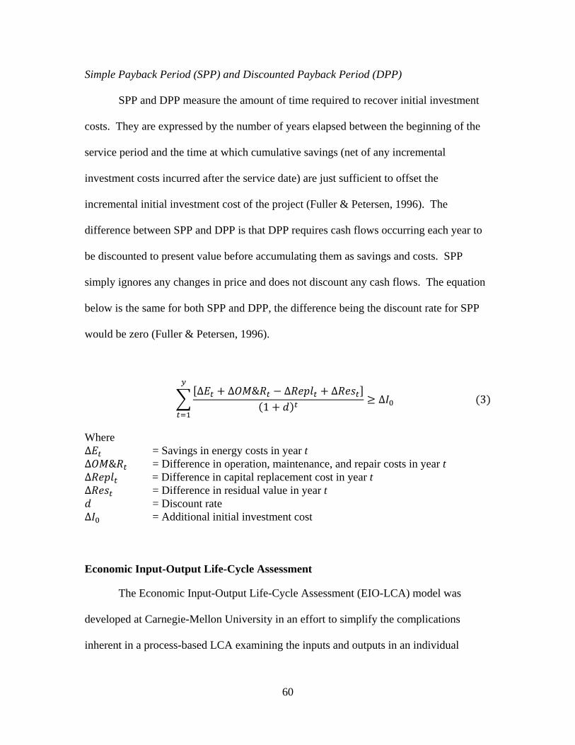
60
Simple Payback Period (SPP) and Discounted Payback Period (DPP)
SPP and DPP measure the amount of time required to recover initial investment
costs. They are expressed by the number of years elapsed between the beginning of the
service period and the time at which cumulative savings (net of any incremental
investment costs incurred after the service date) are just sufficient to offset the
incremental initial investment cost of the project (Fuller & Petersen, 1996). The
difference between SPP and DPP is that DPP requires cash flows occurring each year to
be discounted to present value before accumulating them as savings and costs. SPP
simply ignores any changes in price and does not discount any cash flows. The equation
below is the same for both SPP and DPP, the difference being the discount rate for SPP
would be zero (Fuller & Petersen, 1996).
∆ ∆ & ∆ ∆1
∆ 3
Where ∆ = Savings in energy costs in year t ∆ & = Difference in operation, maintenance, and repair costs in year t ∆ = Difference in capital replacement cost in year t ∆ = Difference in residual value in year t
= Discount rate ∆ = Additional initial investment cost
Economic Input-Output Life-Cycle Assessment
The Economic Input-Output Life-Cycle Assessment (EIO-LCA) model was
developed at Carnegie-Mellon University in an effort to simplify the complications
inherent in a process-based LCA examining the inputs and outputs in an individual

61
product’s life-cycle. Process-based LCA is very accurate for simple products like paper
drinking cups; however, it becomes much more difficult when multiple items are
combined to make one product, as in the case of street lamps. Finding the information
necessary for this type of LCA is nearly impossible and creates boundary issues for the
study. Therefore, the EIO-LCA model uses economic input-output matrices and industry
sector level environmental and nonrenewable resource consumption data to assess the
economy-wide environmental impacts of products and processes (Hendrickson, Horvath,
Joshi, Klausner, Lave, & McMichael, 1997). The Economic Input-Output (EIO) model
uses mathematical formulas to represent the monetary transactions between industry
sectors associated with a product’s life-cycle, from the acquisition of raw materials to
create the product to the end-of-life disposal of that product. EIO models indicate what
goods or services (or output of an industry) are consumed by other industries (or used as
input) (Carnegie-Mellon University, 2008).
EIO models identify the direct, indirect, and total effects of changes to the
economy. Direct effects are the first-tier transactions between a sector and the sectors
that provide its direct output. For example, the power production sector would be
directly affected by coal mining, as coal is a primary source for power production.
Indirect effects are the second-tier, third-tier, etc., transactions among all sectors as a
result of the first-tier transactions. Total effects are the sum of direct and indirect effects
(Carnegie-Mellon University, 2008). Utilizing an input-output approach to conduct
LCA, EIO-LCA utilizes sectors classified by the North American Industry Classification
System (NAICS) in conjunction with economic data tables derived from the Bureau of
Economic Analysis (BEA) and publicly available environmental data from the EPA and

62
the Department of Energy (DOE) (Huang & Matthews, 2008). The environmental data
linked to these tables provides data about the pollutants resulting from the economic
activity associated with each sector involved in the life-cycle of a given product. The
pollutants tracked are measured in metric tons and consist of the following: methane
(CH4), carbon dioxide (CO2), nitrous oxide (N2O), and chlorofluorocarbons (CFC). The
combination of these pollutants creates an overall global warming potential (GWP) which
was used to determine the overall environmental impact associated with the life-cycle of
each lighting technology.
In order to streamline the use of EIO-LCA, Carnegie-Mellon University’s Green
Design Institute has created an online tool to determine the effect of changing the output
of a single sector through multiple models based on different years. This tool facilitates
the use of models for analysis and allows for customized models to be developed for
custom and hybrid products. A custom model was used to analyze how the difference in
materials between the lighting technologies affects environmental impact over the
material processing, manufacturing, and disposal phases.
Using the EIO-LCA model
EIO-LCA was used in this study to assess the environmental impacts associated
with the material processing, manufacturing, and disposal phases of the different lighting
technologies. The lighting technologies were compared by analyzing the differences
between them, as there are many similarities throughout the product life of the lighting
technologies. These differences were input into the EIO-LCA model and the levels of
change between environmental and economic impacts were compared. Because of the

63
complexity associated with this model, every change in input can have a significant effect
on the level and types of impact across all tiers and sectors. In order to minimize the
number of affects possible across the 490 sectors associated with EIO-LCA, only the top
10 were analyzed for comparing direct and indirect emissions. This reduced the number
of variables in the matrix calculation and allowed for a more streamlined analysis.
Inputs for the EIO-LCA Software
In order for the EIO-LCA software to calculate an accurate output, it was
important to determine which NAICS sectors were going to be used as inputs for this
study. Based on the findings in the literature review, the sectors shown in Table 9 were
the corresponding inputs for each phase of the life-cycle associated with each lighting
technology.
Table 9. EIO-LCA Input Data
Fixture Type Manufacturing Phase Use Phase Disposal PhaseHPS Electric Lamp Bulb and Part
Manufacturing (100%)BLCC Emissions CO2
Waste Management and Remediation
Cost = $54 per bulb Hazardous Disposal Cost = $1.50 per bulbEOL Fixture Disposal = $2.50 per fixture
LED Lighting Fixture Manufacturing (20%)
BLCC Emissions CO2
Waste Management and Remediation
Semiconductor and Related Device Manufacturing (80%)
Fixture Disposal Cost Year 11 = $1 per fixture
Cost = $354 per fixture EOL Fixture Disposal = $1 per fixtureHPS Fixture Disposal = $2.50 per fixture
Induction Lighting Fixture Manufacturing (100%)
BLCC Emissions CO2
Waste Management and Remediation
Cost = $499 per fixture EOL Fixture Disposal Cost = $1 per fixtureEOL Hazardous Disposal Cost = $1.50 per fixtureHPS Fixture Disposal = $2.50 per fixture
*EOL - End of Life

64
Manufacturing Phase
Based on the information obtained during the literature review, the following
assumptions were made about each lighting technology. For HPS, the only sector to
include in the manufacturing phase was the Electric Lamp Bulb and Part Manufacturing
sector because this study only looked at replacing the light bulbs at their replacement
interval. The electrodeless induction fixtures are essentially the equivalent of fluorescent
lamps, so the Lighting Fixture Manufacturing sector was used. Because this lighting
fixture will last the duration of the study, they only needed to be manufactured once. For
LED fixtures, a combination of the Semiconductor and Related Device Manufacturing
sector was used at 80% and the Lighting Fixture Manufacturing sector was used at 20%.
This breakdown was used because the majority of an LED fixture (LEDs, power supply,
circuit board) is recognized in the semiconductor sector. However, other aspects, such as
the fixture housing and wiring, are highlighted under the lighting fixture sector. These
percentages are an approximation, as the content of the different LED fixtures on the
market may vary. Because of the equipment service life associated with the LED
technology, they were manufactured twice for this study.
The costs associated with each of these technologies were assumed to have a 25%
profit already built into the cost of each bulb or fixture. This additional profit was
removed for this analysis to allow a more realistic estimate of the actual cost required to
produce each of these lighting technologies. The GWP emissions and fixture costs for
each technology multiplied by the total number of fixtures in use by the Air Force will
result in the total GWP emissions for this phase. The total number of fixtures at each
location can be found in Appendix A.

65
Use Phase
The use phase was calculated using the BLCC5 emissions output data. The data
provided by the BLCC5 software provides a more accurate estimation of CO2 emissions
output for each individual location than EIO-LCA can provide. The variance in CO2
between states is significant enough to warrant a more detailed analysis than EIO-LCA
can provide. These CO2 emissions combined with the total number of fixtures will
produce the GWP for this phase.
Disposal Phase
The Waste and Remediation Services sector was used to calculate the disposal
costs for all three technologies. HPS bulbs require disposal every four years and incur an
additional cost associated with the disposal of mercury inside the bulbs. The HPS fixture
also incurs a fixture disposal cost at the end of the study, as it is assumed the fixture will
require replacement at that time. Both LED and electrodeless induction include the cost
for the disposal of the original HPS fixtures, as these disposal costs help increase the
accuracy of the study. Because the equipment service life for LED does not reach the
end of the study period, disposal costs were calculated for fixture disposal at the 11 year
point and at the end of the study. The electrodeless induction fixtures have an equipment
service life that takes them through the end of the study, so only one disposal fee related
to these fixtures is necessary. An additional cost was levied on the electrodeless
induction fixture for hazardous waste disposal as a result of the mercury used in the
induction bulb. The average disposal fee for an HID light source due to its classification
as hazardous waste is $2.50/lamp (EHSO, 2010). This disposal fee was split to segregate

66
fixture disposal cost and hazardous material cost. This additional cost was included in
the Waste and Remediation Services sector during the analysis. The GWP emissions for
fixture and bulb disposal combined with the total number of fixtures will produce the
GWP results for this phase of the analysis.
Summary
This chapter has detailed the methodology used in this study. Using both LCCA
and EIO-LCA allowed for a more thorough analysis than using either one as the sole
method for this study. The analysis provided by the BLCC5 software allowed for a
clearer analysis of the advantages/disadvantages associated with each technology over the
long-term for the use phase both economically and environmentally. The environmental
results from the BLCC5 along with the results from the EIO-LCA model helped analyze
the environmental costs and energy usage associated with each lighting technology from
the manufacturing phase of product life through to the disposal phase. This helped
identify any tradeoffs associated with the lighting technologies between the energy
savings and environmental emissions.

67
IV. Results and Analysis
This chapter details the results of this study to compare high pressure sodium
(HPS), electrodeless induction, and light-emitting diode (LED) street lighting
technologies. The first section of the chapter analyzes the data used in the study along
with relevant operation and installation costs. The second section focuses on the
economic impacts associated with the technologies. Life-cycle costs for each technology
will also be determined, to include the use of sensitivity analysis to examine the effects of
equipment design life, fixture prices, power consumption, and carbon emission offset
expenses. The third section of the chapter focuses on the environmental impacts
associated with each technology. The economic input-output life-cycle assessment (EIO-
LCA) tool will be used to analyze the environmental impacts associated with each
technology as they relate to the overall economy. This study covers 56 independent
locations covering 30 states, 4 countries, and the District of Columbia.
Economic Impact
Using the information given in earlier chapters, an economic analysis was
performed to determine which lighting technology provided the best cost-benefit over the
study period. The economic measures used for comparison included the savings-to-
investment ratio, adjusted internal rate of return, simple payback period, and the
discounted payback period. These values were calculated by comparing HPS fixtures to
LED and electrodeless induction fixtures of equivalent performance. The intention of
this analysis was to determine whether the newer technologies with their higher upfront

68
costs and lower power usage were economically viable. These comparisons were made
without the use of tax incentives or emissions penalties, as policies relating to these
aspects can change over time. Emissions penalties are discussed later in this chapter.
Savings-to-Investment Ratio Results
The savings to investment ratio calculates how much money can be saved
compared to the amount invested. An SIR of 1.0 means that the money invested is equal
to the money saved. The Air Force has mandated a minimum SIR of 1.25 for energy
projects. Table 10 shows the results from calculating the savings-to-investment ratio for
each of the newer lighting technologies compared with its HPS equivalent fixture at each
location. Table 11 displays the summary results for the entire study. The SIR
comparison shows that both LED and induction technologies will have a decent return on
investment when used to replace HPS lighting. There are seven locations at which LED
technology and three locations at which induction technology would have an SIR under
1.0, suggesting these locations would lose money when investing in the newer
technology. On the other hand, there are 10 locations at which LED technology and 12
locations at which induction technology would have an SIR greater than 2.0, suggesting
that investing in the newer technologies at these locations would provide significant cost
savings over HPS technology. With LED having an SIR so close to the Air Force
requirement of 1.25 along with the 0.58 standard deviation, LED would be a difficult
technology to suggest based on this measure. Induction is a more viable alternative for
replacement, as its SIR is 0.19 higher while its standard deviation only increased by 0.06.

69
Table 10. Savings-to-Investment Ratio Compared with Similar HPS Fixture
Base Name LED IND Base Name LED INDALTUS AFB 1.22 1.34 KIRTLAND AFB 1.41 1.52ANDREWS AFB 1.69 1.86 KUNSAN AB 1.38 1.51BARKSDALE AFB 1.05 1.14 LACKLAND AFB 1.24 1.42BEALE AFB 1.09 1.27 LANGLEY AFB 1.24 1.42BOLLING AFB 2.00 2.19 LAUGHLIN AFB 1.88 2.07BUCKLEY AFB 1.24 1.41 LOS ANGELES AFS 1.69 1.90CANNON AFB 1.16 1.32 LUKE AFB 1.26 1.26CAPE CANAVERAL 1.49 1.68 MALMSTROM AFB 1.34 1.52CHARLESTON AFB 1.13 1.28 MCCHORD AFB 0.90 1.08CLEAR AFS 3.31 3.70 MCCONNELL AFB 1.14 1.29DAVIS MONTHAN AFB 1.24 1.41 MCGUIRE AFB 2.04 2.26DYESS AFB 1.39 1.55 MINOT AFB 0.94 1.13EARECKSON 2.76 3.12 MISAWA AB 1.75 1.91EDWARDS AFB 2.06 2.31 MOODY AFB 1.23 1.42EGLIN AFB 1.73 1.93 MT HOME AFB 0.83 0.99EIELSON AFB 2.21 2.48 NELLIS AFB 1.23 1.43ELLSWORTH AFB 0.92 1.06 OFFUTT AFB 0.84 0.98ELMENDORF AFB 1.11 1.31 ROBINS AFB 1.15 1.31FAIRCHILD AFB 0.85 1.00 SCHRIEVER AFB 1.26 1.45GOODFELLOW AFB 1.07 1.19 SCOTT AFB 1.08 1.23GRAND FORKS AFB 1.04 1.23 SEYMOUR JOHNSON AFB 1.29 1.49HANSCOM AFB 2.07 2.32 SHEPPARD AFB 1.59 1.76HICKAM AFB 2.62 2.91 THULE AB 3.07 3.41HILL AFB 0.74 0.89 TRAVIS AFB 1.04 1.24HOLLOMAN AFB 1.32 1.50 USAF ACADEMY 1.01 1.16HURLBURT FLD 1.49 1.73 VANDENBERG AFB 1.35 1.51KEESLER AFB 1.33 1.49 WHITEMAN AFB 1.05 1.24KING SALMON 2.97 3.35 YOKOTA AB 1.84 2.03
Table 11. Savings-to-Investment Summary
Fixture Type Low High Average Std Deviation Met AF RequirementLED 0.74 3.31 1.47 0.58 29Induction 0.89 3.70 1.66 0.64 42

70
Adjusted Internal Rate of Return Results
The adjusted internal rate of return is the overall rate of return on the investment
to include installation, operations, maintenance, and disposal costs associated with each
lighting technology. This minimum allowable rate of return (MARR) must exceed 7% in
order to cover the cost of capital used according to the Office of Management and Budget
(OMB, 1992). Other entities and organizations may require a different discount rate
depending on the funding source, but the Air Force is bound to the OMB rate. Table 12
shows the results from the AIRR analysis per location while Table 13 summarizes the
results. The AIRR analysis is not supportive of these new technologies. Only 15
locations for LED and 17 locations for induction meet or exceed the MARR for this
study. Both technologies have an average AIRR below the minimum required, although
induction does have a slight edge over LED in this measure.

71
Table 12. Adjusted Internal Rate of Return
Base Name LED IND Base Name LED INDALTUS AFB 5.26% 5.77% KIRTLAND AFB 6.02% 6.44%ANDREWS AFB 6.99% 7.51% KUNSAN AB 5.93% 6.40%BARKSDALE AFB 4.47% 4.90% LACKLAND AFB 5.37% 6.08%BEALE AFB 4.66% 5.48% LANGLEY AFB 5.37% 6.09%BOLLING AFB 7.91% 8.41% LAUGHLIN AFB 7.59% 8.10%BUCKLEY AFB 5.38% 6.06% LOS ANGELES AFS 7.00% 7.63%CANNON AFB 5.02% 5.68% LUKE AFB 5.44% 5.44%CAPE CANAVERAL 6.33% 6.99% MALMSTROM AFB 5.78% 6.43%CHARLESTON AFB 4.88% 5.55% MCCHORD AFB 3.67% 4.63%CLEAR AFS 10.66% 11.29% MCCONNELL AFB 4.91% 5.58%DAVIS MONTHAN AFB 5.34% 6.04% MCGUIRE AFB 8.02% 8.58%DYESS AFB 5.97% 6.56% MINOT AFB 3.93% 4.87%EARECKSON 9.67% 10.34% MISAWA AB 7.19% 7.66%EDWARDS AFB 8.08% 8.69% MOODY AFB 5.31% 6.09%EGLIN AFB 7.13% 7.73% MT HOME AFB 3.25% 4.16%EIELSON AFB 8.46% 9.07% NELLIS AFB 5.30% 6.11%ELLSWORTH AFB 3.82% 4.56% OFFUTT AFB 3.34% 4.14%ELMENDORF AFB 4.77% 5.67% ROBINS AFB 4.99% 5.36%FAIRCHILD AFB 3.37% 4.25% SCHRIEVER AFB 5.44% 6.21%GOODFELLOW AFB 4.59% 5.13% SCOTT AFB 4.63% 5.32%GRAND FORKS AFB 4.44% 5.34% SEYMOUR JOHNSON AFB 5.58% 6.34%HANSCOM AFB 8.09% 8.72% SHEPPARD AFB 6.68% 7.23%HICKAM AFB 9.38% 9.95% THULE AB 10.24% 10.84%HILL AFB 2.70% 3.61% TRAVIS AFB 4.43% 5.34%HOLLOMAN AFB 5.69% 6.36% USAF ACADEMY 4.28% 5.00%HURLBURT FLD 6.35% 7.13% VANDENBERG AFB 5.80% 6.41%KEESLER AFB 5.74% 6.35% WHITEMAN AFB 4.49% 5.38%KING SALMON 10.07% 10.74% YOKOTA AB 7.46% 1.99%
Table 13. Adjusted Internal Rate of Return Results Summary
Fixture Type Low High Average Std Deviation Met AF RequirementLED 2.70% 10.66% 5.94% 1.85% 15Induction 1.99% 11.29% 6.50% 1.88% 17

72
Simple Payback Period Results
The simple payback period is another measure of a project’s financial feasibility
and is commonly used in government estimates. It represents the number of years, based
on operating cost savings, required to pay back the initial investment amount associated
with the project. Table 14 shows the results of the simple payback analysis per location
with Table 15 displaying the summarized results. The Air Force recommends a simple
payback period that is under 10 years for energy projects. Using this Air Force criterion,
52 locations for LED and 29 locations for induction are able to meet the goal. Looking at
the average and standard deviation values for each technology, LED has the advantage as
its average is lower than the minimum SPP required and the first standard deviation is
still within the allowable payback period. The average for the induction technology is 10
years, putting it right on the line of financial feasibility.
This analysis also shows that some bases can payback the financial investment in
these new technologies relatively quickly. The shortest payback period for LED is 3
years, which occurs at three locations; however, 4 years is the earliest payback period for
induction, which occurs at only one location. There is also one instance in which the
payback period for LED technology is not realized in the lifetime of the study. Draft
ETL 10-02 suggests reducing the SPP for LED lighting to 5 years in order to coincide
with the typical warranty period offered by manufacturers for this technology. If the SPP
is reduced to 5 years, only 12 locations would reach the required SPP for implementation.

73
Table 14. Simple Payback Period Results per Location (Years)
Base Name LED IND Base Name LED INDALTUS AFB 8 11 KIRTLAND AFB 7 10ANDREWS AFB 6 9 KUNSAN AB 7 10BARKSDALE AFB 9 13 LACKLAND AFB 8 11BEALE AFB 8 12 LANGLEY AFB 8 11BOLLING AFB 5 7 LAUGHLIN AFB 5 8BUCKLEY AFB 7 11 LOS ANGELES AFS 6 8CANNON AFB 8 11 LUKE AFB 12 12CAPE CANAVERAL 6 9 MALMSTROM AFB 7 10CHARLESTON AFB 8 12 MCCHORD AFB 10 13CLEAR AFS 3 4 MCCONNELL AFB 8 12DAVIS MONTHAN AFB 7 11 MCGUIRE AFB 5 7DYESS AFB 7 10 MINOT AFB 10 13EARECKSON 4 5 MISAWA AB 6 8EDWARDS AFB 5 7 MOODY AFB 8 11EGLIN AFB 6 8 MT HOME AFB 11 15EIELSON AFB 4 6 NELLIS AFB 7 10ELLSWORTH AFB 10 14 OFFUTT AFB 11 15ELMENDORF AFB 8 11 ROBINS AFB 8 11FAIRCHILD AFB 10 14 SCHRIEVER AFB 7 10GOODFELLOW AFB 9 13 SCOTT AFB 9 12GRAND FORKS AFB 9 12 SEYMOUR JOHNSON AFB 7 10HANSCOM AFB 5 7 SHEPPARD AFB 6 9HICKAM AFB 4 6 THULE AB 3 5HILL AFB - 16 TRAVIS AFB 9 12HOLLOMAN AFB 7 10 USAF ACADEMY 9 13HURLBURT FLD 6 9 VANDENBERG AFB 7 10KEESLER AFB 7 10 WHITEMAN AFB 9 12KING SALMON 3 5 YOKOTA AB 5 8
Table 15. Simple Payback Results Summary
Fixture Type Low High Average Std Deviation Met AF RequirementLED 3 >20 7 3 52Induction 4 16 10 3 29

74
Discounted Payback Period Results
This discounted payback period is similar to SPP with the exception that the time
value of money is taken into account, which is important when comparing items with
larger initial costs and lower operating costs over time. The results for the DPP analysis
at each location are shown in Table 16 with the summarized results shown in Table 17.
The results for DPP show slightly longer payback periods than those seen in SPP, which
is to be expected. With the time value of money accounted for, there are seven locations
for LED and three locations for induction that show no payback over the study period.
The shortest payback period is 3 years for one location using the LED technology, while
the shortest payback period for induction has increased to 5 years, which occurs at three
locations are capable of reaching. The averages for each technology have increased by 2
and 3 years for LED and induction lighting, respectively.

75
Table 16. Discounted Payback Period Results per Location (Years)
Base Name LED IND Base Name LED INDALTUS AFB 9 14 KIRTLAND AFB 7 12ANDREWS AFB 6 10 KUNSAN AB 8 13BARKSDALE AFB 10 18 LACKLAND AFB 9 13BEALE AFB 10 15 LANGLEY AFB 9 13BOLLING AFB 5 9 LAUGHLIN AFB 6 9BUCKLEY AFB 8 13 LOS ANGELES AFS 6 10CANNON AFB 9 15 LUKE AFB 15 15CAPE CANAVERAL 7 11 MALMSTROM AFB 8 12CHARLESTON AFB 10 15 MCCHORD AFB - 19CLEAR AFS 3 5 MCCONNELL AFB 10 15DAVIS MONTHAN AFB 9 13 MCGUIRE AFB 6 8DYESS AFB 8 12 MINOT AFB - 18EARECKSON 4 6 MISAWA AB 6 10EDWARDS AFB 5 8 MOODY AFB 9 13EGLIN AFB 6 10 MT HOME AFB - -EIELSON AFB 5 7 NELLIS AFB 9 13ELLSWORTH AFB - 19 OFFUTT AFB - -ELMENDORF AFB 10 15 ROBINS AFB 9 15FAIRCHILD AFB - 20 SCHRIEVER AFB 8 13GOODFELLOW AFB 10 17 SCOTT AFB 10 16GRAND FORKS AFB 11 16 SEYMOUR JOHNSON AFB 8 13HANSCOM AFB 5 8 SHEPPARD AFB 7 11HICKAM AFB 4 6 THULE AB 4 5HILL AFB - - TRAVIS AFB 10 16HOLLOMAN AFB 8 13 USAF ACADEMY 11 17HURLBURT FLD 7 11 VANDENBERG AFB 8 12KEESLER AFB 8 13 WHITEMAN AFB 10 16KING SALMON 4 5 YOKOTA AB 6 9
Table 17. Discounted Payback Period Results Summary
Fixture Type Low High Average Std DeviationLED 3 >20 9 5Induction 5 >20 13 4
76
Emissions Results
Although the BLCC5 software is mostly used for cost analysis, it is also capable
of calculating the carbon dioxide (CO2), sulfur dioxide (SO2), and nitrous oxide (NOX).
Because it was assumed that each lighting technology would perform similarly at each
base, the differences in output for these greenhouse gases was based on each state or
country in which the military base is located. Each state or country has a slightly
different way of producing power, resulting in differing greenhouse gas emissions. For
this portion of the analysis, only CO2 output was recorded, as this is what was used to
calculate the carbon tax at each location. The results are shown graphically by state or
country in Figure 15 and by base in Table 18. These results show a significant carbon
footprint for the HPS technology in comparison with LED and induction technologies.
LED technology produces 55% less emissions while the induction technology produces
45% less emissions compared to HPS. States such as Idaho and California produce the
least amount of emissions at just fewer than 700kg of CO2 per year for a single HPS
fixture while North Dakota and the District of Columbia are the highest CO2 emitters at
around 1500kg of CO2 per year for the same fixture.
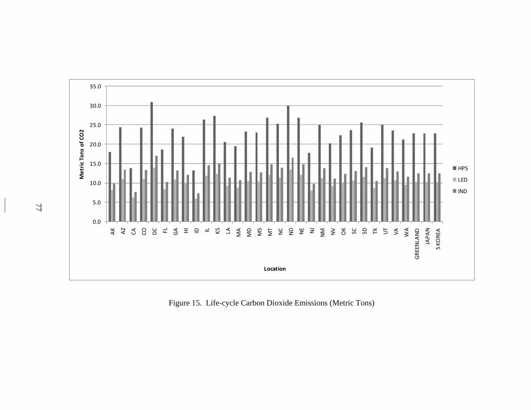
77
Figure 15. Life-cycle Carbon Dioxide Emissions (Metric Tons)
0.0
5.0
10.0
15.0
20.0
25.0
30.0
35.0
AK
AZ
CA
CO
DC FL GA HI
ID IL KS
LA MA
MD
MS
MT
NC
ND NE NJ
NM NV
OK
SC SD TX UT
VA
WA
GREENLA
ND
JAPAN
S KOREA
Metric Tons of C
O2
Location
HPS
LED
IND

78
Table 18. CO2 Emissions Data by Location Singe Fixture (Metric Tons)
Base Name Annual Life-Cycle Annual Life-Cycle Annual Life-CycleALTUS AFB 1.1 22.3 0.5 10.1 0.6 12.3ANDREWS AFB 1.2 23.3 0.5 10.5 0.6 12.8BARKSDALE AFB 1.0 20.6 0.5 9.3 0.6 11.3BEALE AFB 0.7 13.8 0.3 6.2 0.4 7.6BOLLING AFB 1.5 30.9 0.7 13.9 0.9 17.0BUCKLEY AFB 1.2 24.3 0.5 10.9 0.7 13.4CANNON AFB 1.3 25.0 0.6 11.3 0.7 13.8CAPE CANAVERAL 0.9 18.6 0.4 8.4 0.5 10.2CHARLESTON AFB 1.2 23.7 0.5 10.7 0.7 13.0CLEAR AFS 0.9 18.0 0.4 8.1 0.5 9.9DAVIS MONTHAN AFB 1.2 24.4 0.5 11.0 0.7 13.4DYESS AFB 1.0 19.1 0.4 8.6 0.5 10.5EARECKSON 0.9 18.0 0.4 8.1 0.5 9.9EDWARDS AFB 0.7 13.8 0.3 6.2 0.4 7.6EGLIN AFB 0.9 18.6 0.4 8.4 0.5 10.3EIELSON AFB 0.9 18.0 0.4 8.1 0.5 9.9ELLSWORTH AFB 1.3 25.6 0.6 11.5 0.7 14.1ELMENDORF AFB 0.9 18.0 0.4 8.1 0.5 9.9FAIRCHILD AFB 1.1 21.2 0.5 9.5 0.6 11.6GOODFELLOW AFB 1.0 19.1 0.4 8.6 0.5 10.5GRAND FORKS AFB 1.5 30.0 0.7 13.5 0.8 16.5HANSCOM AFB 1.0 19.5 0.4 8.8 0.5 10.7HICKAM AFB 1.1 21.9 0.5 9.8 0.6 12.0HILL AFB 1.3 25.0 0.6 11.3 0.7 13.8HOLLOMAN AFB 1.3 25.1 0.6 11.3 0.7 13.8HURLBURT FLD 0.9 18.6 0.4 8.4 0.5 10.3KEESLER AFB 1.2 23.1 0.5 10.4 0.6 12.7KING SALMON 0.9 18.0 0.4 8.1 0.5 9.9KIRTLAND AFB 1.3 25.1 0.6 11.3 0.7 13.8KUNSAN AB 1.1 22.7 0.5 10.2 0.6 12.5LACKLAND AFB 1.0 19.2 0.4 8.6 0.5 10.5LANGLEY AFB 1.2 23.6 0.5 10.6 0.6 13.0LAUGHLIN AFB 1.0 19.2 0.4 8.6 0.5 10.5LOS ANGELES AFS 0.7 13.8 0.3 6.2 0.4 7.6LUKE AFB 1.2 24.4 0.5 11.0 0.7 13.4MALMSTROM AFB 1.3 26.8 0.6 12.1 0.7 14.8MCCHORD AFB 1.1 21.1 0.5 9.5 0.6 11.6MCCONNELL AFB 1.4 27.3 0.6 12.3 0.8 15.0MCGUIRE AFB 0.9 17.7 0.4 8.0 0.5 9.7MINOT AFB 1.5 30.0 0.7 13.5 0.8 16.5MISAWA AB 1.1 22.7 0.5 10.2 0.6 12.5MOODY AFB 1.2 24.0 0.5 10.8 0.7 13.2MT HOME AFB 0.7 13.2 0.3 5.9 0.4 7.2NELLIS AFB 1.0 20.2 0.5 9.1 0.6 11.1OFFUTT AFB 1.3 26.9 0.6 12.1 0.7 14.8ROBINS AFB 1.2 24.0 0.5 10.8 0.7 13.2SCHRIEVER AFB 1.2 24.3 0.5 10.9 0.7 13.4SCOTT AFB 1.3 26.4 0.6 11.9 0.7 14.5SEYMOUR JOHNSON AFB 1.3 25.3 0.6 11.4 0.7 13.9SHEPPARD AFB 1.0 19.2 0.4 8.6 0.5 10.5THULE AB 1.1 22.7 0.5 10.2 0.6 12.5TRAVIS AFB 0.7 13.8 0.3 6.2 0.4 7.6USAF ACADEMY 1.2 24.3 0.5 10.9 0.7 13.4VANDENBERG AFB 0.7 13.8 0.3 6.2 0.4 7.6WHITEMAN AFB 1.4 27.3 0.6 12.3 0.8 15.0YOKOTA AB 1.1 22.7 0.5 10.2 0.6 12.5
INDLEDHPS
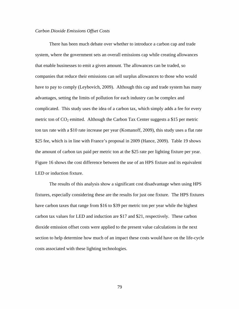
79
Carbon Dioxide Emissions Offset Costs
There has been much debate over whether to introduce a carbon cap and trade
system, where the government sets an overall emissions cap while creating allowances
that enable businesses to emit a given amount. The allowances can be traded, so
companies that reduce their emissions can sell surplus allowances to those who would
have to pay to comply (Leybovich, 2009). Although this cap and trade system has many
advantages, setting the limits of pollution for each industry can be complex and
complicated. This study uses the idea of a carbon tax, which simply adds a fee for every
metric ton of CO2 emitted. Although the Carbon Tax Center suggests a $15 per metric
ton tax rate with a $10 rate increase per year (Komanoff, 2009), this study uses a flat rate
$25 fee, which is in line with France’s proposal in 2009 (Hance, 2009). Table 19 shows
the amount of carbon tax paid per metric ton at the $25 rate per lighting fixture per year.
Figure 16 shows the cost difference between the use of an HPS fixture and its equivalent
LED or induction fixture.
The results of this analysis show a significant cost disadvantage when using HPS
fixtures, especially considering these are the results for just one fixture. The HPS fixtures
have carbon taxes that range from $16 to $39 per metric ton per year while the highest
carbon tax values for LED and induction are $17 and $21, respectively. These carbon
dioxide emission offset costs were applied to the present value calculations in the next
section to help determine how much of an impact these costs would have on the life-cycle
costs associated with these lighting technologies.

80
Table 19. Annual Carbon Tax per Fixture
Base Name HPS LED IND Base Name HPS LED INDALTUS AFB $28 $13 $15 KIRTLAND AFB $31 $14 $17ANDREWS AFB $29 $13 $16 KUNSAN AB $28 $13 $16BARKSDALE AFB $26 $12 $14 LACKLAND AFB $24 $11 $13BEALE AFB $17 $8 $9 LANGLEY AFB $29 $13 $16BOLLING AFB $39 $17 $21 LAUGHLIN AFB $24 $11 $13BUCKLEY AFB $30 $14 $17 LOS ANGELES AFS $17 $8 $9CANNON AFB $31 $14 $17 LUKE AFB $30 $14 $17CAPE CANAVERAL $23 $10 $13 MALMSTROM AFB $34 $15 $18CHARLESTON AFB $30 $13 $16 MCCHORD AFB $26 $12 $15CLEAR AFS $22 $10 $12 MCCONNELL AFB $34 $15 $19DAVIS MONTHAN AFB $30 $14 $17 MCGUIRE AFB $22 $10 $12DYESS AFB $24 $11 $13 MINOT AFB $37 $17 $21EARECKSON $22 $10 $12 MISAWA AB $28 $13 $16EDWARDS AFB $17 $8 $9 MOODY AFB $30 $13 $16EGLIN AFB $23 $10 $13 MT HOME AFB $16 $7 $9EIELSON AFB $22 $10 $12 NELLIS AFB $25 $11 $14ELLSWORTH AFB $32 $14 $18 OFFUTT AFB $34 $15 $18ELMENDORF AFB $22 $10 $12 ROBINS AFB $30 $13 $16FAIRCHILD AFB $26 $12 $15 SCHRIEVER AFB $30 $14 $17GOODFELLOW AFB $24 $11 $13 SCOTT AFB $33 $15 $18GRAND FORKS AFB $37 $17 $21 SEYMOUR JOHNSON AFB $32 $14 $17HANSCOM AFB $24 $11 $13 SHEPPARD AFB $24 $11 $13HICKAM AFB $27 $12 $15 THULE AB $28 $13 $16HILL AFB $31 $14 $17 TRAVIS AFB $17 $8 $9HOLLOMAN AFB $31 $14 $17 USAF ACADEMY $30 $14 $17HURLBURT FLD $23 $10 $13 VANDENBERG AFB $17 $8 $9KEESLER AFB $29 $13 $16 WHITEMAN AFB $34 $15 $19KING SALMON $22 $10 $12 YOKOTA AB $28 $13 $16
Life-Cycle Cost Results
Another important aspect of this study was to examine the life-cycle cost
associated with each of these lighting technologies. Present value analysis accounts for
the total life-cycle costs incurred for the installation, operation, and maintenance of each
lighting fixture type over the 20-year service period. Table 20 shows the present value
for a single lighting fixture at each location. Table 21 summarizes the results and Figure
16 graphically expresses the cost savings, comparing HPS technology to LED and

81
induction technology. The PV calculations show a cost savings of 21% and 23% for
LED and induction technologies, respectively, when compared to HPS. LED has the best
PV savings at 15 locations in this study, with 7 locations showing a negative savings;
induction technology has the best PV for 38 locations, with only 3 locations showing a
negative savings. HPS shows a cost advantage over the other technologies at 3 locations.
Table 20. Present Value Cost for Single Fixture
Base Name HPS LED IND Base Name HPS LED IND
ALTUS AFB $1,746 $1,549 $1,500 KIRTLAND AFB $1,940 $1,587 $1,575ANDREWS AFB $2,640 $1,978 $1,992 KUNSAN AB $2,040 $1,676 $1,647BARKSDALE AFB $1,463 $1,418 $1,355 LACKLAND AFB $1,849 $1,608 $1,523BEALE AFB $1,710 $1,619 $1,492 LANGLEY AFB $1,855 $1,613 $1,526BOLLING AFB $3,097 $2,145 $2,205 LAUGHLIN AFB $2,895 $2,055 $2,095BUCKLEY AFB $1,829 $1,591 $1,513 LOS ANGELES AFS $2,688 $1,978 $1,970CANNON AFB $1,653 $1,499 $1,417 LUKE AFB $1,559 $1,457 $1,365CAPE CANAVERAL $2,304 $1,815 $1,771 MALMSTROM AFB $1,998 $1,665 $1,604CHARLESTON AFB $1,602 $1,476 $1,389 MCCHORD AFB $1,269 $1,377 $1,206CLEAR AFS $6,083 $3,553 $3,833 MCCONNELL AFB $1,613 $1,482 $1,395DAVIS MONTHAN AFB $1,821 $1,589 $1,507 MCGUIRE AFB $3,269 $2,240 $2,299DYESS AFB $2,047 $1,675 $1,631 MINOT AFB $1,359 $1,420 $1,254EARECKSON $5,104 $3,136 $3,310 MISAWA AB $2,604 $1,911 $1,936EDWARDS AFB $3,215 $2,165 $2,207 MOODY AFB $1,864 $1,630 $1,530EGLIN AFB $2,709 $1,989 $1,992 MT HOME AFB $1,106 $1,280 $1,117EIELSON AFB $3,718 $2,463 $2,542 NELLIS AFB $1,884 $1,649 $1,542ELLSWORTH AFB $1,238 $1,311 $1,190 OFFUTT AFB $1,101 $1,252 $1,115ELMENDORF AFB $1,694 $1,579 $1,436 ROBINS AFB $1,650 $1,501 $1,415FAIRCHILD AFB $1,135 $1,288 $1,133 SCHRIEVER AFB $1,919 $1,654 $1,560GOODFELLOW AFB $1,427 $1,364 $1,295 SCOTT AFB $1,511 $1,436 $1,339GRAND FORKS AFB $1,547 $1,506 $1,357 SEYMOUR JOHNSON AFB $1,984 $1,684 $1,596HANSCOM AFB $3,443 $2,341 $2,393 SHEPPARD AFB $2,390 $1,829 $1,819HICKAM AFB $4,469 $2,798 $2,952 THULE AB $5,460 $3,259 $3,493HILL AFB $941 $1,192 $1,028 TRAVIS AFB $1,549 $1,508 $1,357HOLLOMAN AFB $1,968 $1,655 $1,588 USAF ACADEMY $1,390 $1,382 $1,273HURLBURT FLD $2,438 $1,909 $1,843 VANDENBERG AFB $1,973 $1,642 $1,591KEESLER AFB $1,946 $1,630 $1,576 WHITEMAN AFB $1,560 $1,508 $1,364KING SALMON $5,504 $3,304 $3,516 YOKOTA AB $2,844 $2,037 $2,067
Table 21. Present Value Cost Results Summary
Fixture Type Low High Average Std Deviation Avg Savings
HPS $941 $6,083 $2,279 $1,154 -
LED $1,192 $3,553 $1,801 $529 $478
IND $1,028 $3,833 $1,760 $628 $519

82
Figure 16. Present Value Savings Compared with HPS
‐$250
$0
$250
$500
$750
$1,000
$1,250
$1,500
$1,750
$2,000
$2,250
$2,500
$2,750
ALTUS AFB
ANDREW
S AFB
BARKSD
ALE AFB
BEA
LE AFB
BOLLING AFB
BUCKLEY AFB
CANNON AFB
CAPE CANAVERAL
CHARLESTON AFB
CLEAR AFS
DAVIS M
ONTH
AN AFB
DYESS AFB
EARECKSO
N
EDWARDS AFB
EGLIN AFB
EIELSO
N AFB
ELLSWORTH
AFB
ELMEN
DORF AFB
FAIRCHILD AFB
GOODFELLOW AFB
GRAND FORKS AFB
HANSCOM AFB
HICKAM AFB
HILL AFB
HOLLOMAN AFB
HURLBURT FLD
KEESLER
AFB
KING SALM
ON
KIRTLAND AFB
KUNSA
N AB
LACKLA
ND AFB
LANGLEY AFB
LAUGHLIN AFB
LOS ANGELES AFS
LUKE AFB
MALM
STROM AFB
MCCHORD AFB
MCCONNELL AFB
MCGUIRE AFB
MINOT AFB
MISAWA AB
MOODY AFB
MT HOME AFB
NELLIS AFB
OFFUTT AFB
ROBINS AFB
SCHRIEVER
AFB
SCOTT AFB
SEYM
OUR JOHNSO
N AFB
SHEPPARD AFB
THULE AB
TRAVIS AFB
USA
F ACADEM
Y
VANDEN
BERG A
FB
WHITEM
AN AFB
YOKOTA
AB
Presen
t Value
Location
LED
IND
GreaterSavings

83
Using this PV data, the approximate savings can be calculated by multiplying the
single fixture PV by the number of fixtures located at each location. Table 22 shows the total
cost savings for LED and induction technology compared to HPS. The total savings for
using LED is approximately $10.9 million over the life-cycle, whereas induction would save
almost $12.6 million over the life-cycle. Converting these life-cycle savings to an annual
cost, the Air Force would save approximately $820 thousand and $940 thousand annually for
the implementation of LED and induction technology, respectively.
Table 22. Present Value Savings for all fixtures
Base Name LED IND Base Name LED INDALTUS AFB $208,229 $260,022 KIRTLAND AFB $143,318 $148,190ANDREWS AFB $1,026,762 $1,005,048 KUNSAN AB $91,000 $98,250BARKSDALE AFB $6,660 $15,984 LACKLAND AFB $383,913 $519,318BEALE AFB $142,961 $342,478 LANGLEY AFB $97,526 $132,587BOLLING AFB $225,624 $211,404 LAUGHLIN AFB $974,400 $928,000BUCKLEY AFB $102,102 $135,564 LOS ANGELES AFS $156,910 $158,678CANNON AFB $113,344 $173,696 LUKE AFB $98,328 $187,016CAPE CANAVERAL $97,800 $106,600 MALMSTROM AFB $373,959 $442,462CHARLESTON AFB $23,436 $39,618 MCCHORD AFB -$71,712 $41,832CLEAR AFS $75,900 $67,500 MCCONNELL AFB $28,427 $47,306DAVIS MONTHAN AFB $91,872 $124,344 MCGUIRE AFB $427,035 $402,550DYESS AFB $186,000 $208,000 MINOT AFB -$7,625 $13,125EARECKSON $177,120 $161,460 MISAWA AB $248,094 $239,144EDWARDS AFB $456,750 $438,480 MOODY AFB $61,542 $87,842EGLIN AFB $180,000 $179,250 MT HOME AFB -$52,200 -$3,300EIELSON AFB $1,316,495 $1,233,624 NELLIS AFB $67,445 $98,154ELLSWORTH AFB -$17,447 $11,472 OFFUTT AFB -$69,913 -$6,482ELMENDORF AFB $105,225 $236,070 ROBINS AFB $89,400 $141,000FAIRCHILD AFB -$88,128 $1,152 SCHRIEVER AFB $90,100 $122,060GOODFELLOW AFB $5,733 $12,012 SCOTT AFB $38,325 $87,892GRAND FORKS AFB $12,956 $60,040 SEYMOUR JOHNSON AFB $162,600 $210,296HANSCOM AFB $287,622 $274,050 SHEPPARD AFB $336,600 $342,600HICKAM AFB $574,824 $521,848 THULE AB $261,919 $234,073HILL AFB -$163,150 -$56,550 TRAVIS AFB $21,279 $99,648HOLLOMAN AFB $82,006 $99,560 USAF ACADEMY $488 $7,137HURLBURT FLD $509,427 $572,985 VANDENBERG AFB $516,029 $595,538KEESLER AFB $317,264 $371,480 WHITEMAN AFB $6,552 $24,696KING SALMON $330,000 $298,200 YOKOTA AB $68,595 $66,045

84
Life-Cycle Costs including Carbon Dioxide Emissions Costs
Using the annual carbon tax values calculated in Table 19, the life-cycle costs for
these technologies at each location were recalculated. The results for each location are
shown in Table 23 with the summarized results in Table 24. Figure 17 displays the PV
differential savings comparing HPS with LED and induction technologies. The results from
this analysis shift the PV for both of the newer technologies even greater in their favor. The
HPS technology saw a $400 increase for its average in the study while LED and induction
technologies saw an increase of approximately $200 in the same category.
The average savings also increased from $478 to $703 for LED technology while the
average savings for induction went from $519 to $703. Also, LED is now the best value at
20 locations, whereas induction is the best value at 36 locations. When the carbon tax was
not present, HPS was the best value at three locations; however, the addition of the carbon
tax gave induction the advantage at these locations. The carbon tax also gave LED an
advantage at five locations where induction previously had the cost advantage. It is also
worth noting that the standard deviation for each technology went down after the addition of
the carbon tax, suggesting that charging for emissions output provides a normalizing affect
on the data.

85
Table 23. Present Value Cost with $25 Carbon Tax
Base Name HPS LED IND Base Name HPS LED IND
ALTUS AFB $2,187 $1,753 $1,736 KIRTLAND AFB $2,395 $1,792 $1,824ANDREWS AFB $3,097 $2,182 $2,244 KUNSAN AB $2,477 $1,878 $1,897BARKSDALE AFB $1,872 $1,607 $1,575 LACKLAND AFB $2,226 $1,781 $1,728BEALE AFB $1,959 $1,736 $1,624 LANGLEY AFB $2,311 $1,818 $1,778BOLLING AFB $3,711 $2,412 $2,535 LAUGHLIN AFB $3,273 $2,228 $2,299BUCKLEY AFB $2,269 $1,796 $1,762 LOS ANGELES AFS $2,917 $2,095 $2,102CANNON AFB $2,108 $1,705 $1,666 LUKE AFB $1,808 $1,575 $1,497CAPE CANAVERAL $2,666 $1,973 $1,975 MALMSTROM AFB $2,496 $1,884 $1,868CHARLESTON AFB $2,074 $1,681 $1,641 MCCHORD AFB $1,650 $1,552 $1,425CLEAR AFS $6,405 $3,699 $4,009 MCCONNELL AFB $2,154 $1,720 $1,697DAVIS MONTHAN AFB $2,261 $1,794 $1,756 MCGUIRE AFB $3,627 $2,403 $2,494DYESS AFB $2,424 $1,848 $1,836 MINOT AFB $1,947 $1,690 $1,588EARECKSON $5,427 $3,282 $3,486 MISAWA AB $3,041 $2,114 $2,186EDWARDS AFB $3,464 $2,282 $2,339 MOODY AFB $2,336 $1,834 $1,782EGLIN AFB $3,071 $2,147 $2,197 MT HOME AFB $1,340 $1,382 $1,249EIELSON AFB $4,055 $2,610 $2,733 NELLIS AFB $2,251 $1,810 $1,747ELLSWORTH AFB $1,746 $1,533 $1,476 OFFUTT AFB $1,641 $1,490 $1,401ELMENDORF AFB $2,017 $1,726 $1,612 ROBINS AFB $2,122 $1,706 $1,667FAIRCHILD AFB $1,516 $1,464 $1,352 SCHRIEVER AFB $2,359 $1,859 $1,810GOODFELLOW AFB $1,804 $1,538 $1,499 SCOTT AFB $2,036 $1,674 $1,625GRAND FORKS AFB $2,135 $1,776 $1,690 SEYMOUR JOHNSON AFB $2,488 $1,904 $1,864HANSCOM AFB $3,834 $2,520 $2,605 SHEPPARD AFB $2,768 $2,002 $2,024HICKAM AFB $4,864 $2,974 $3,172 THULE AB $5,897 $3,461 $3,743HILL AFB $1,396 $1,397 $1,277 TRAVIS AFB $1,798 $1,625 $1,489HOLLOMAN AFB $2,422 $1,860 $1,837 USAF ACADEMY $1,830 $1,587 $1,522HURLBURT FLD $2,800 $2,066 $2,047 VANDENBERG AFB $2,222 $1,760 $1,723KEESLER AFB $2,402 $1,835 $1,828 WHITEMAN AFB $2,100 $1,746 $1,666KING SALMON $5,826 $3,451 $3,692 YOKOTA AB $3,281 $2,240 $2,316
Table 24. Present Value Cost with $25 Carbon Tax Results Summary
Fixture Type Low High Average Std Deviation Avg Savings
HPS $1,340 $6,405 $2,689 $1,134 -
LED $1,382 $3,699 $1,987 $520 $703
IND $1,249 $4,009 $1,986 $618 $703

86
Figure 17. Present Value Savings with Carbon Tax
‐$200
$0
$200
$400
$600
$800
$1,000
$1,200
$1,400
$1,600
$1,800
$2,000
$2,200
$2,400
$2,600
$2,800
ALTUS AFB
ANDREW
S AFB
BARKSD
ALE AFB
BEA
LE AFB
BOLLING AFB
BUCKLEY AFB
CANNON AFB
CAPE CANAVERAL
CHARLESTON AFB
CLEAR AFS
DAVIS M
ONTH
AN AFB
DYESS AFB
EARECKSO
N
EDWARDS AFB
EGLIN AFB
EIELSO
N AFB
ELLSWORTH
AFB
ELMEN
DORF AFB
FAIRCHILD AFB
GOODFELLOW AFB
GRAND FORKS AFB
HANSCOM AFB
HICKAM AFB
HILL AFB
HOLLOMAN AFB
HURLBURT FLD
KEESLER
AFB
KING SALM
ON
KIRTLAND AFB
KUNSA
N AB
LACKLA
ND AFB
LANGLEY AFB
LAUGHLIN AFB
LOS ANGELES AFS
LUKE AFB
MALM
STROM AFB
MCCHORD AFB
MCCONNELL AFB
MCGUIRE AFB
MINOT AFB
MISAWA AB
MOODY AFB
MT HOME AFB
NELLIS AFB
OFFUTT AFB
ROBINS AFB
SCHRIEVER
AFB
SCOTT AFB
SEYM
OUR JOHNSO
N AFB
SHEPPARD AFB
THULE AB
TRAVIS AFB
USA
F ACADEM
Y
VANDEN
BERG A
FB
WHITEM
AN AFB
YOKOTA
AB
Presen
t Value
Location
LED
INDGreaterSavings

87
Life-Cycle Cost Sensitivity Analysis Results
Life-cycle cost is one of the better tools for measuring project feasibility and
comparison; however, it can be impacted by several factors. It is important to investigate
these factors in order to have a full understanding of how sensitive this analysis was to
changes in the values of these factors. The factors that were investigated are equipment
service life, fixture cost, power consumption, and carbon tax rates. Each of these factors was
studied separately and the results can be found in the following sections.
All 56 locations in this study were analyzed, but five locations were chosen for
additional discussion. The locations were selected based on their utility costs, labor costs,
and carbon dioxide emission rates. Locations representing both the upper and lower limits of
each of these factors were chosen for this analysis. Hill AFB had the lowest utility rate in
this study, Kirtland AFB had the lowest labor rate, and Mt Home AFB had the lowest carbon
dioxide emissions offset rate. Clear AFS had one of the higher labor rates and utility rates,
while Bolling AFB had the highest carbon dioxide emissions offset rate. All bases were not
used in all sensitivity analyses, as some bases had similar utility and labor rates. The
sensitivity analysis was calculated using the BLCC5 software used in the previous section.
Equipment Service Life Sensitivity Results
There has been much discussion as to how long these newer lighting technologies
will actually last. Possible problems with the high-frequency generators in the induction
fixtures and power supply issues with the LED fixtures may cause these lighting technologies
to fail prematurely. Understanding how premature failure could affect the life-cycle cost is
important, as the likelihood of these lighting technologies not lasting their claimed service

88
life is well within reason. To conduct this analysis, the PV cost was calculated for each new
lighting technology with equipment service lives of 5, 10, and 20 years. No salvage values
were attributed to fixtures whose equipment service life went beyond the 20-year study
period. A study of less than 5 years would be unnecessary, as both induction and LED
fixtures have minimum 5-year warranties. The results for three different scenarios are shown
in Figures 18 through 20.
Figure 18. Equipment Service Life Sensitivity with Low Utility Rate (Hill AFB)
$0
$500
$1,000
$1,500
$2,000
$2,500
$3,000
0 5 10 15 20 25
Presen
t Value
Cost
Equipment Service Life (years)
HPS
LED
IND

89
Figure 19. Equipment Service Life Sensitivity with Low Labor Rate (Kirtland AFB)
Figure 20. Equipment Service Life Sensitivity with High Utility and Labor Rate (Clear AFS)
$0
$500
$1,000
$1,500
$2,000
$2,500
$3,000
$3,500
0 5 10 15 20 25
Presen
t Value
Cost
Equipment Service Life (years)
HPS
LED
IND
$0
$1,000
$2,000
$3,000
$4,000
$5,000
$6,000
$7,000
0 5 10 15 20 25
Presen
t Value
Cost
Equipment Service Life (years)
HPS
LED
IND

90
The results show that the longer the equipment service life, the lower the PV cost for
the newer technologies. LED has a better PV cost than induction at the shorter service life
intervals. As the service life increases, induction begins to close the gap with LED; however,
a breakeven point is not realized in this analysis. The low utility rate location shows a
negative savings for both technologies until the 20-year service life is reached; at that point,
only LED surpasses HPS as the most cost-effective. The low labor rate location shows both
LED and induction to be less cost-effective than HPS at the 5-year service life. LED
becomes more cost-effective at the 10-year service life, and induction does not surpass HPS
until the 20-year service life. The high utility and labor rate location shows payback for both
technologies at the 5-year service period.
Fixture Cost Sensitivity Analysis
The continuous improvements for both LED and induction technologies has increased
production efficiency and reduced production costs, which are usually reflected in lower
retail fixture costs. However, increases in raw material prices or supply shortages can
adversely affect the cost of these lighting technologies. Understanding the sensitivity of
fixture cost fluctuations can help determine the overall economic viability and flexibility
these new technologies offer. To perform this analysis, the fixture costs for the induction and
LED lighting technologies were changed between +10% and -50% of the current cost and the
range of present value costs were calculated as shown in Table 25. Figures 21 through 23
show the outputs associated with these price variations.

91
Table 25. Values used for Fixture Cost Sensitivity Analysis
Fixture Type 10% 0% -10% -20% -30% -40% -50%LED $519 $472 $425 $378 $330 $283 $236IND $732 $665 $599 $532 $466 $399 $333
Figure 21. Fixture Cost Sensitivity with Low Utility Rate (Hill AFB)
$0
$200
$400
$600
$800
$1,000
$1,200
$1,400
10% 0% ‐10% ‐20% ‐30% ‐40% ‐50%
Presen
t Value
Cost
Percent Change in Fixture Cost
HPS
LED
IND
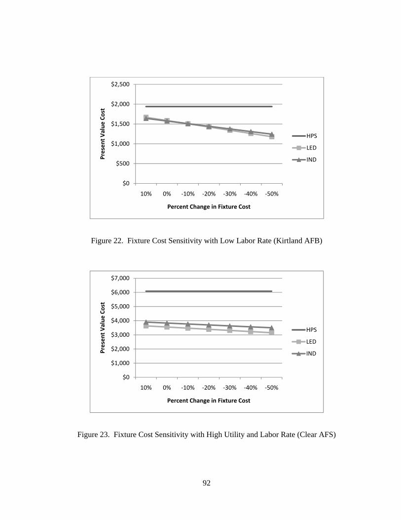
92
Figure 22. Fixture Cost Sensitivity with Low Labor Rate (Kirtland AFB)
Figure 23. Fixture Cost Sensitivity with High Utility and Labor Rate (Clear AFS)
$0
$500
$1,000
$1,500
$2,000
$2,500
10% 0% ‐10% ‐20% ‐30% ‐40% ‐50%
Presen
t Value
Cost
Percent Change in Fixture Cost
HPS
LED
IND
$0
$1,000
$2,000
$3,000
$4,000
$5,000
$6,000
$7,000
10% 0% ‐10% ‐20% ‐30% ‐40% ‐50%
Presen
t Value
Cost
Percent Change in Fixture Cost
HPS
LED
IND

93
These results show that given certain price points, the economic viability of a certain
lighting technology will change compared with other lighting technologies. The low utility
rate location shows that induction lighting will be more cost effective than HPS if the fixture
price drops by 15% or more; similarly, the LED fixture price will need to drop by 30% or
more before it is more cost effective than HPS. Both the low labor rate location and high
utility and labor rate location show both LED and induction technologies being more cost-
effective than HPS for the complete range of price variations. These locations also show that
at a certain percentage, LED will become more cost-effective than induction. The low labor
rate location illustrates this behavior the best; although induction is initially the most cost
effective technology, the LED technology becomes more cost-effective when the fixture cost
drops by 20% or more.
Power Consumption Sensitivity Analysis
Because the power consumption was estimated, this could call into question the
ability of these lighting technologies to perform similarly, as each Air Force base is slightly
different. Therefore, this sensitivity analysis varies the amount of power consumed by each
fixture in the study from -30% to +30% from the nominal values and calculates the
associated present value costs. The nominal values used for all technologies were based on
the nominal rating for the lamps themselves; no line losses or input requirements were
considered. Table 26 displays the values used for this analysis with Figures 24 through 26
displaying the results of this analysis.

94
Table 26. Nominal Values for Power Sensitivity Analysis
Percentage250W HPS
250W LED 250W Ind
-30% 163 92 109-20% 192 105 122-10% 221 118 1350% 250 131 15010% 279 144 16520% 308 157 18030% 337 170 195
Figure 24. Power Consumption Sensitivity with Low Utility Rate (Hill AFB)
$0
$200
$400
$600
$800
$1,000
$1,200
$1,400
‐30% ‐20% ‐10% 0% 10% 20% 30%
Presen
t Value
Cost
Percent Change in Power Consumption
HPS
LED
IND
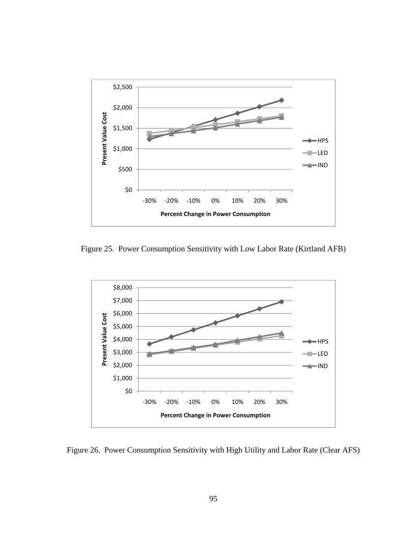
95
Figure 25. Power Consumption Sensitivity with Low Labor Rate (Kirtland AFB)
Figure 26. Power Consumption Sensitivity with High Utility and Labor Rate (Clear AFS)
$0
$500
$1,000
$1,500
$2,000
$2,500
‐30% ‐20% ‐10% 0% 10% 20% 30%
Presen
t Value
Cost
Percent Change in Power Consumption
HPS
LED
IND
$0
$1,000
$2,000
$3,000
$4,000
$5,000
$6,000
$7,000
$8,000
‐30% ‐20% ‐10% 0% 10% 20% 30%
Presen
t Value
Cost
Percent Change in Power Consumption
HPS
LED
IND

96
This analysis shows a linear rise in present value costsfor each technology as the
power consumption increases. The slope of each plot is directly related to power
consumption; therefore, HPS has the steepest rise in cost while LED has the flattest cost
increase. It should be noted that a power consumption lower than the nominal rate used in
this analysis for the HPS technology is highly unlikely; however, it has been graphed in order
to show present value trends and also to represent what type of affect a lower power HPS
fixture would have on this study. The same case can be made for LED and induction
technologies as well, although the DOE CALiPER test showed both technologies operating
below their rated power (DOE, 2009).
The low utility rate location shows that HPS remains more cost-effective than the
LED and induction technologies throughout the range of power consumption values. The
low labor rate location shows a close grouping of all three technologies as power
consumption values decrease; however, as power consumption increases, HPS becomes the
least cost-effective of the three technologies. At 30% above nominal, LED and induction
technologies have a similar PV cost. The high utility and labor rate location shows both
induction and LED having an advantage over HPS throughout the range of power
consumption values. HPS is only competitive if the power consumption decreased by 30%
and both the induction and LED increased at least 10% ; however, such a scenario is highly
unlikely.

97
Carbon Dioxide Emissions Cost Sensitivity Analysis
The previous section showed the PV results after incorporating a $25 carbon emission
offset cost with each lighting technology. While these costs are currently not being
implemented, better understanding the affect of a carbon emission offset cost can help
forecast how significant the introduction of this cost will be. This sensitivity analysis varies
the carbon emission offset costs from $0 to $100 per metric ton of CO2. Figures 27 through
31 are a graphical presentation of the present values associated with the differing carbon
emission offset costs.
Figure 27. Carbon Emission Offset Cost Sensitivity with Low Utility Rate (Hill AFB)
$0
$500
$1,000
$1,500
$2,000
$2,500
$3,000
$0 $20 $40 $60 $80 $100 $120
Presen
t Value
Cost
Carbon Tax Cost per Metric Ton CO2
HPS
LED
IND

98
Figure 28. Carbon Emission Offset Cost Sensitivity with Low Labor Rate (Kirtland AFB)
Figure 29. Carbon Emission Offset Cost Sensitivity with High Utility and Labor Rate (Clear AFS)
$0
$500
$1,000
$1,500
$2,000
$2,500
$3,000
$3,500
$4,000
$0 $20 $40 $60 $80 $100 $120
Presen
t Value
Cost
Carbon Tax per Metric Ton CO2
HPS
LED
IND
$0
$1,000
$2,000
$3,000
$4,000
$5,000
$6,000
$7,000
$8,000
$0 $20 $40 $60 $80 $100 $120
Presen
t Value
Cost
Carbon Tax Cost Per Metric Ton CO2
HPS
LED
IND

99
Figure 30. Carbon Emission Offset Cost Sensitivity for Low CO2 Emission Location (Mt Home AFB)
Figure 31. Carbon Emission Offset Cost Sensitivity for High CO2 Emission Location (Bolling AFB)
$0
$500
$1,000
$1,500
$2,000
$2,500
$0 $20 $40 $60 $80 $100 $120
Presen
t Value
Cost
Carbon Tax Cost per Metric Ton CO2
HPS
LED
IND
$0
$1,000
$2,000
$3,000
$4,000
$5,000
$6,000
$0 $20 $40 $60 $80 $100 $120
Presen
t Value
Cost
Carbon Tax per Metric Ton CO2
HPS
LED
IND

100
The results of this analysis show the sensitivity of HPS technology to the carbon
emission offset cost compared with LED and induction technology. The low utility rate
location shows an almost 200% increase in PV costs when the $100 per metric ton CO2
carbon tax is added to HPS compared to no carbon tax. The affects on LED and induction
are not as dramatic as those for HPS; however, the increase for both technologies is
approximately 100% when compared to the $0 carbon tax value. The graph also shows the
induction and LED lines converging as the carbon tax rises, with LED becoming more cost-
effective when the tax exceeds $100 per metric ton CO2.
The low labor rate location shows both LED and induction starting at approximately
the same point; as the carbon tax increases though, the LED technology becomes slightly
more cost-effective. The high utility and labor rate location shows LED and induction
almost parallel to each other as the carbon tax amount rises, with LED being the most cost
effective. Both LED and induction technologies are clearly more cost effective than HPS
throughout the range of emissions values.
For the low CO2 emissions location, induction and HPS have similar PV costs with
LED being less cost-effective. As the carbon tax increases to about $30 per metric ton CO2,
HPS becomes less cost-effective compared to the LED technology. As the carbon tax
surpasses $100, the LED and induction plots begin to converge; however, induction remains
the most cost-effective. The results for the high CO2 emissions rate location are very similar
to those of the low labor rate location, with a 44% increase in PV costs for HPS, 38%
increase for induction, and 34% increase for LED over the range of carbon tax values.
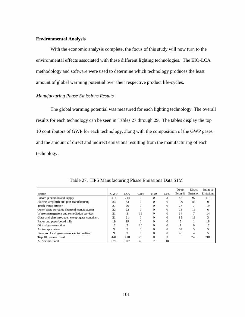
101
Environmental Analysis
With the economic analysis complete, the focus of this study will now turn to the
environmental effects associated with these different lighting technologies. The EIO-LCA
methodology and software were used to determine which technology produces the least
amount of global warming potential over their respective product life-cycles.
Manufacturing Phase Emissions Results
The global warming potential was measured for each lighting technology. The overall
results for each technology can be seen in Tables 27 through 29. The tables display the top
10 contributors of GWP for each technology, along with the composition of the GWP gases
and the amount of direct and indirect emissions resulting from the manufacturing of each
technology.
Table 27. HPS Manufacturing Phase Emissions Data $1M
Sector GWP CO2 CH4 N20 CFCDirect
Econ %Direct
EmissionIndirect
Emissions
Power generation and supply 216 214 0 0 3 45 97 119Electric lamp bulb and part manufacturing 83 83 0 0 0 100 83 0Truck transportation 27 26 0 0 0 27 7 19Other basic inorganic chemical manufacturing 22 22 0 0 0 73 16 6Waste management and remediation services 21 3 18 0 0 34 7 14Glass and glass products, except glass containers 21 21 0 0 0 85 18 3Paper and paperboard mills 19 19 0 0 0 5 1 18Oil and gas extraction 12 2 10 0 0 1 0 12Air transportation 9 9 0 0 0 52 5 5State and local government electric utilities 9 9 0 0 0 46 4 5Top 10 Sectors Total 441 410 28 0 3 240 201All Sectors Total 576 507 45 7 18

102
Table 28. Induction Manufacturing Phase Emissions Data $1M
Sector GWP CO2 CH4 N20 CFCDirect
Econ %Direct
EmissionsIndirect
Emissions
Power generation and supply 188 186 0 0 2 23 43 145Iron and steel mills 64 64 0 0 0 50 32 32Lighting fixture manufacturing 47 47 0 0 0 100 47 0Truck transportation 47 46 0 1 0 42 20 27Primary aluminum production 32 11 0 0 21 4 1 30Waste management and remediation services 25 4 21 0 0 27 7 18Paper and paperboard mills 17 17 0 0 0 10 2 15Oil and gas extraction 12 2 10 0 0 0 0 12Coal mining 12 1 11 0 0 1 0 12Air transportation 11 11 0 0 0 46 5 6Top 10 Sectors Total 454 388 42 1 23 156 297All Sectors Total 624 530 51 7 35
Table 29. LED Manufacturing Phase Emissions Data $1M
Sector GWP CO2 CH4 N20 CFCDirect
Econ %Direct
EmissionIndirect
Emissions
Power generation and supply 141 139 0 0 2 42 59 82Semiconductors and related device manufacturing 80 9 0 0 71 87 70 10Industrial gas manufacturing 53 15 0 0 38 73 39 14Iron and steel mills 19 19 0 0 0 32 6 13Truck transportation 18 18 0 0 0 32 6 12Other basic inorganic chemical manufacturing 17 17 0 0 0 68 11 5Waste management and remediation services 16 3 14 0 0 39 6 10Primary nonferrous metal, except copper and aluminum 10 1 0 0 10 67 7 3Lighting fixture manufacturing 9 9 0 0 0 33 3 6Primary aluminum production 9 3 0 0 6 15 1 7Top 10 Sectors Total 372 232 14 0 126 208 164All Sectors Total 482 320 31 5 126
These values were calculated using an economic input of $1 million for each lighting
technology to ensure a fair comparison was performed between manufacturing processes.
After analyzing the data, the lowest GWP per $1 million between the three lighting
technologies is LED manufacturing. At 482 metric tons of CO2 equivalence, LED
manufacturing not only has the lowest GWP, but it is also responsible for the smallest
amount of indirect emissions, suggesting most of the emissions being produced from the
manufacturing of LEDs is directly attributed to the production of LEDs and not lost in
residual sectors surrounding the LEDs. Induction lighting manufacturing had the worst

103
environmental impact of the three options, producing 624 metric tons of CO2 equivalent
emissions for every $1 million of production.
Comparing these technologies on an equal scale allows for a direct comparison of
manufacturing processes. While the environmental impact from manufacturing each
technology is important, the three technologies do not have the same cost factors associated
with them. The costs associated with each lighting technology affects how many fixtures can
be produced for a given cost. Table 30 shows the total environmental impact given the costs
for each technology and the Air Force requirements for those technologies. Figure 32 is the
graphical representation of Table 30.
Table 30. Manufacturing Phase Emissions
Fixture Type Fixture Cost Replacement# of
FixturesTotal Cost
($M)GWP per
$1M Total GWP
HPS $54 4 28910 $6.24 576 3600LED $354 2 28910 $20.47 482 9900IND $499 1 28910 $14.43 624 9000

104
Figure 32. Manufacturing Phase Emissions
These results show that the manufacturing of HPS bulbs has a much lower
environmental impact compared to either of the new technologies over the study period.
This can be attributed directly to the low cost of the bulbs. Even if they need to be replaced
every 4 years, the replacement cost is approximately one-seventh the cost of the other
technologies, allowing more bulbs to be produced for less money and fewer emissions. The
LED technology, despite having the most emissions-efficient manufacturing process,
produced the highest GWP in this phase. This is the direct result of the equipment service
0
2000
4000
6000
8000
10000
12000
HPS LED IND
Globa
l Warming Po
tential in Metric To
n CO
2 Eq
uivalent

105
life, which requires twice the number of fixtures to be made compared to the induction
technology.
Use Phase Emissions Results
The use phase emissions were calculated using the BLCC5 software during the
economic analysis. Table 31 displays the results of the emissions calculations and Figure 33
represents them graphically. The results show the LED and induction technologies have a
significant advantage in life-cycle emissions over HPS, producing 55% and 45% fewer
emissions than HPS, respectively.
Table 31. Total Air Force Life-Cycle Carbon Dioxide Emissions per Location (Metric Tons)
Base Name HPS LED IND Base Name HPS LED IND
ALTUS AFB 23613 10626 12987 KIRTLAND AFB 10174 4578 5596ANDREWS AFB 36138 16262 19876 KUNSAN AB 5685 2558 3127BARKSDALE AFB 3052 1373 1678 LACKLAND AFB 30522 13735 16787BEALE AFB 21680 9756 11924 LANGLEY AFB 9495 4273 5222BOLLING AFB 7333 3300 4033 LAUGHLIN AFB 22226 10002 12224BUCKLEY AFB 10425 4691 5734 LOS ANGELES AFS 3050 1372 1677CANNON AFB 18429 8293 10136 LUKE AFB 23502 10576 12926CAPE CANAVERAL 3724 1676 2048 MALMSTROM AFB 30141 13564 16578CHARLESTON AFB 4404 1982 2422 MCCHORD AFB 14037 6317 7720CLEAR AFS 539 242 296 MCCONNELL AFB 5924 2666 3258DAVIS MONTHAN AFB 9654 4345 5310 MCGUIRE AFB 7346 3305 4040DYESS AFB 9570 4307 5264 MINOT AFB 3745 1685 2060EARECKSON 1616 727 889 MISAWA AB 8141 3663 4478EDWARDS AFB 6003 2701 3302 MOODY AFB 6307 2838 3469EGLIN AFB 4660 2097 2563 MT HOME AFB 3954 1779 2175EIELSON AFB 18840 8478 10362 NELLIS AFB 5792 2606 3185ELLSWORTH AFB 6128 2758 3370 OFFUTT AFB 12445 5600 6845ELMENDORF AFB 16433 7395 9038 ROBINS AFB 14388 6475 7913FAIRCHILD AFB 12188 5485 6703 SCHRIEVER AFB 8262 3718 4544GOODFELLOW AFB 1742 784 958 SCOTT AFB 13480 6066 7414GRAND FORKS AFB 9467 4260 5207 SEYMOUR JOHNSON AFB 13713 6171 7542HANSCOM AFB 5095 2293 2802 SHEPPARD AFB 11496 5173 6323HICKAM AFB 7527 3387 4140 THULE AB 2706 1218 1488HILL AFB 16276 7324 8952 TRAVIS AFB 7162 3223 3939HOLLOMAN AFB 6566 2955 3611 USAF ACADEMY 1482 667 815HURLBURT FLD 17950 8078 9873 VANDENBERG AFB 21514 9681 11833KEESLER AFB 23152 10419 12734 WHITEMAN AFB 3440 1548 1892KING SALMON 2694 1212 1482 YOKOTA AB 1933 870 1063
Total 607,000 275,000 335,000

106
Figure 33. Use Phase Emissions
Disposal Phase Emissions Results
The disposal phase uses the Waste Management and Remediation Services sector for
calculating the total GWP associated with the disposal of these lighting technologies. Table
32 shows the results for $1 million worth of waste disposal and Table 33 calculates the GWP
for each lighting technology, the results of which are shown graphically in Figure 34.
0
100,000
200,000
300,000
400,000
500,000
600,000
700,000
HPS LED IND
CO2 in M
etric To
ns

107
Table 32. Global Warming Potential for $1M Waste Disposal
Sector GWP CO2 CH4 N20 CFCDirect
Econ %Direct
EmissionsIndirect
Emissions
Waste management and remediation services 6800 1075 5717 8 0 98 6678 122Power generation and supply 249 246 0 0 3 66 164 85Oil and gas extraction 42 7 35 0 0 4 2 40Petroleum refineries 36 36 0 0 0 70 25 11Truck transportation 31 31 0 0 0 57 18 14Pipeline transportation 19 9 10 0 0 9 2 17Industrial gas manufacturing 15 4 0 0 11 70 10 4Air transportation 11 11 0 0 0 61 7 4State and local government electric utilities 10 10 0 0 0 64 6 4Natural gas distribution 8 2 6 0 0 71 6 2Top 10 Sectors Total 7220 1431 5768 9 14 6916 304All Sectors Total 7310 1500 5780 17 15
Table 33. Disposal Phase Emissions Calculation
Fixture TypeBulb Disposal
Cost
Fixture Disposal
CostBulb
DisposalFixture
Disposals # of Fixtures Total CostGWP per
$1MBulb Disposal
GWP
Fixture Disposal
GWPInitial HPS Disposal
Total GWP
HPS $1.50 $1.00 4 1 28910 $173,460 7310 1300 500 - 1800LED - $1.00 - 2 28910 $57,820 7310 - 400 500 900IND $1.50 $1.00 - 1 28910 $72,275 7310 - 500 500 1000
Figure 34. Disposal Phase Emissions
0
200
400
600
800
1,000
1,200
1,400
1,600
1,800
2,000
HPS LED IND
Globa
l Warming Po
tential in Metric
Tons CO2 Eq
uivalent

108
These results show that the HPS technology has the highest GWP in this phase,
producing 50% more emissions than LED and 45% more emissions than induction; however,
compared to the other two phases, the differences between the three technologies are very
small. Despite having to dispose of the LED fixtures twice and the induction fixtures once,
the LED technology proved to be the most environmentally friendly.
Total Combined Emissions
The total combined emission output for all three phases was calculated for each
technology. The total results are displayed in Table 34 with the distribution for each phase
represented graphically in Figure 35. The use phase for these lighting technologies is by far
the most significant in this study, producing 96%, 97%, and 99% of all the emissions for
LED, induction, and HPS technologies, respectively. Overall, the LED technology produced
the least amount of emissions by roughly 60,000 metric tons of CO2 equivalence when
compared with induction technology. HPS technology was by far the highest producer of
emissions, producing over 600,000 metric tons of CO2 equivalent emissions. When
comparing LED and induction technologies to HPS, they were 54% and 44% more
environmentally friendly than HPS, respectively.
Table 34. Total GWP for Lighting Technologies
Manufacturing Use DisposalHPS 3,600 607,000 1,800 612,400 LED 9,900 275,000 900 285,800 IND 9,000 335,000 1,000 345,000
Total GWPFixture TypePhase

109
Figure 35. Life-Cycle Emissions for each Lighting Technology
0
100,000
200,000
300,000
400,000
500,000
600,000
700,000
HPS LED IND
Globa
l Warming Po
tential in Metric To
ns
of CO2 Eq
uivalent

110
V. Discussion
Summary
This research effort sought to find answers to several questions regarding the
economic and environmental costs of changing roadway and parking lot street lighting
technology across the Air Force. Issues such as installation costs, maintenance costs,
operating costs, energy use, carbon dioxide emissions, and overall life-cycle costs were
explored in this study. The literature review established a need for the research to be
conducted based on government policy and a lack of available studies on both the economic
and environmental aspects of street lighting. The methodology explained how the Building
Life Cycle Cost 5 (BLCC5) and Economic Input-Output Life Cycle Assessment (EIO-LCA)
software were applied to complete this study. The results section detailed the economic and
environmental findings in this study and modeled the sensitivity of certain cost factors for
each lighting technology.
Conclusions
This study provided an in-depth analysis on 56 Air Force installations around the
world with regard to the economic and environmental impacts associated with three different
street lighting technologies. There is significant variability between the electricity and labor
costs on military installations as opposed to the local area, so these results are not necessarily
applicable to the local areas surrounding these installations.
The high-pressure sodium (HPS) technology is on average more costly to operate
than either induction or light-emitting diode (LED) technologies. The calculations for energy

111
use in this study showed a significant difference between the three technologies. Comparing
250W HPS fixtures to induction and LED fixtures of equivalent performance, the induction
fixture consumes 40% less energy while an LED fixture consumes 48% less energy. These
energy savings became more pronounced and resulted in greater financial savings as utility
rates increased.
This study utilized several financial measures to assess the value of LED and
induction lighting. The savings-to-investment ratio (SIR) was used to determine the ratio
between money saved versus money spent. The results showed an average SIR of 1.47 for
the LED technology and 1.66 for the induction technology. These results suggest an
economic advantage when investing in newer technologies, as the energy savings outweigh
the upfront costs associated with these newer technologies.
The discounted payback period (DPP) determines the length of time it takes for the
initial investment in either the LED or induction technology to be recouped when taking into
account the time value of money. The results showed an average of 7 years for the LED
technology and 10 years for the induction technology. Since both technologies have a
significantly high cost of entry, the energy savings were not as large as expected, although
the payback period for many locations still met the Air Force requirement of 10 years or less.
The DPP was most negatively affected at locations where utility costs were low. These low
utility costs give HPS a financial advantage over the newer technologies, as some locations
did not reach payback within the study period with the newer technologies.
The life-cycle costs were also evaluated through the use of present value calculations.
These PV calculations showed an advantage for both induction and LED technologies,

112
averaging a 23% and 21% savings over the HPS technology, respectively. On a per fixture
basis, the LED technology averaged a $478 benefit over HPS while the induction technology
averaged a $519 benefit. These savings may not seem all that significant on a fixture for
fixture basis over a 20-year period; however, when the amount of fixtures utilized by the Air
Force is taken into account, these savings are attractive. The total 250W fixture count for all
the Air Force bases in this study is 28,910 fixtures. The resulting savings for using the LED
technology would be just under $11 million for LED and just over $12.5 million for the
induction technology.
Studying the life-cycle environmental impact associated with these technologies
through the manufacturing, use, and disposal phases was also a key component of this study.
Through the use of EIO-LCA, it was determined that LEDs had the largest global warming
potential in the manufacturing phase. During the use phase, the emissions were significantly
higher for the HPS technology than they were for either induction or LED technology. The
HPS emissions were about double those of LED and induction. The use phase was also the
most significant phase of the three phases, producing between 96% and 99% of all the
emissions in the product life-cycle for each technology. The disposal phase displayed a
relatively small GWP for all three technologies, with HPS contributing the most GWP in this
phase. Across the three phases, it is clear that HPS is the higher emitter of pollutants when
compared to both LED and induction. The difference between LED and induction emissions
is relatively small when looking at the big picture.
Overall, the study showed that both LED and induction technologies are worthy
investments when compared with HPS. LED and induction technologies are both more

113
economically viable and more environmentally friendly. The only situations under which
economic viability comes into question are when utility rates are extremely low. The low
utility rates offset the economic disadvantages associated with the high power consumption
of HPS fixtures, making the introduction of newer technologies less likely with their
prolonged DPP and negligible SIR in these locations. However, from an environmental
standpoint, there is no doubt that HPS fixtures are creating a more significant carbon
footprint than the other two technologies, indirectly contributing to environmental issues
such as air pollution and mercury contamination.
Limitations and Future Research
Although this study addresses some of the shortcomings of other studies, there are
still areas that can be improved or expanded upon. Four major areas could be further
developed to refine the results obtained in this study.
1. The results used in this analysis were estimated values inferred from manufacturer
data and DOE test data. Collecting actual usage data from more Air Force
installations and other case studies using the same fixtures would allow for a more
accurate depiction of how these newer technologies will perform under real-world
conditions. Although the power consumption data used for this study was consistent
with what was found in other studies using similar technologies, it is difficult to
determine whether these particular results represent actual performance.
2. Investigating level of service issues surrounding parking lot and roadway lighting
could yield some interesting results. This study assumed the entire lighting
infrastructure was necessary, suggesting each fixture identified in the study would be

114
used and that the same amount of lighting intensity would be needed. What would
the impact be if every third street lamp along a roadway were eliminated? What if
150W HPS fixtures were used in place of 250W fixtures? Would this change in
wattage be a more cost-effective measure than changing to a newer technology?
3. This study assumed all the lighting technologies would be running at 100% of their
lighting output. With both LED and induction technologies having dimming
capabilities, future research could look into the cost-effectiveness of certain types of
controls, such as proximity and ambient lighting sensors, which reduce power usage
in situations where the lights are not needed.
4. Although economic and environmental factors were researched in this study, a
combination of these factors could be used to address the element of social cost.
Social costs are costs associated with the emissions of GWP. These costs take into
account environmental remediation and health costs associated with variable levels of
GWP emissions. Combining the life-cycle costs for street lighting with the cost of
life-cycle emissions produced by each lighting technology could show a true overall
cost to the government for implementing different lighting technologies.
Recommendations
The Air Force would benefit greatly from both LED and induction lighting
technologies. This study shows that energy and maintenance dollars can be saved by moving
away from HPS technology and adopting either of these newer technologies. However,
before these technologies are adopted on a wide scale at each installation, there should be
pilot tests performed at each base to ensure that the lights are providing the energy and

115
maintenance savings that are expected. One factor to take into account prior to
implementation is the electric utility rate. Table 35 shows the most cost-effective technology
based on the utility rates found in this study. These rates suggest that HPS is only viable
where utility rates are very low, whereas induction lighting is good for places with middle-
of-the-road utility rates. Induction is a good choice in this range because of its long service
life and lower power consumption when compared to HPS. LEDs benefit from higher utility
rates because they are efficient enough to make up for the cost difference and only need to be
replaced every 11 years when compared to the HPS technology. As energy markets fluctuate
and utility costs begin to rise, it becomes less likely that bases with extremely low utility
rates will be able to maintain them, thereby giving these newer lighting technologies a
chance to make a difference both economically and environmentally.
Table 35. Lighting Technology Recommendation
Utility Rate Most Cost-Effectivex < $0.032 HPS
$0.033< x < $0.09 Inductionx > $0.10 LED
While both the induction and LED technologies show great promise, there are still
longevity and compatibility issues associated with each of these technologies. Each base
should take into account its own infrastructure and lighting needs prior to making any
lighting changes. With solid research, pilot, and implementation programs, the introduction
of these new technologies could be a huge success for both the Air Force and the U.S.
government.

116
Appendix A. Air Force Data Call Information
Base Name Location Command Shop RateUtility Rate
(kwh) 250W Fixtures
ALTUS AFB OK AETC $31.58 0.070 1057ANDREWS AFB MD OTHER $45.93 0.112 1551BARKSDALE AFB LA ACC $69.18 0.050 148BEALE AFB CA ACC $74.45 0.066 1571BOLLING AFB DC OTHER $42.00 0.132 237BUCKLEY AFB CO AFSPC $48.79 0.073 429CANNON AFB NM AFSOC $42.00 0.065 736CAPE CANAVERAL FL AFSPC $56.57 0.090 200CHARLESTON AFB SC AMC $42.00 0.058 186CLEAR AFS AK AFSPC $83.86 0.292 30DAVIS MONTHAN AFB AZ ACC $50.87 0.072 396DYESS AFB TX ACC $42.00 0.080 500EARECKSON AK PACAF $90.00 0.24 90EDWARDS AFB CA AFMC $52.00 0.140 435EGLIN AFB FL AFMC $51.56 0.111 250EIELSON AFB AK PACAF $65.57 0.17 1049ELLSWORTH AFB SD ACC $39.76 0.040 239ELMENDORF AFB AK PACAF $77.74 0.06 915FAIRCHILD AFB WA AMC $54.13 0.035 576GOODFELLOW AFB TX AETC $22.25 0.053 91GRAND FORKS AFB ND AMC $73.00 0.049 316HANSCOM AFB MA AFMC $65.26 0.140 261HICKAM AFB HI PACAF $65.00 0.21 344HILL AFB UT AFMC $47.75 0.026 650HOLLOMAN AFB NM ACC $50.50 0.080 262HURLBURT FLD FL AFSOC $76.00 0.093 963KEESLER AFB MS AETC $42.00 0.075 1004KING SALMON AK PACAF $90.00 0.26 150KIRTLAND AFB NM AFMC $18.30 0.085 406KUNSAN AB S KOREA PACAF $44.09 0.08 250LACKLAND AFB TX AETC $53.80 0.068 1593LANGLEY AFB VA ACC $55.36 0.068 403LAUGHLIN AFB TX AETC $42.00 0.122 1160LOS ANGELES AFS CA AFSPC $56.57 0.116 221LUKE AFB AZ AETC $42.00 0.060 964MALMSTROM AFB MT AFSPC $48.58 0.082 1123MCCHORD AFB WA AMC $69.81 0.039 664MCCONNELL AFB KS AMC $42.00 0.058 217MCGUIRE AFB NJ AMC $52.37 0.134 415MINOT AFB ND ACC $72.00 0.040 125MISAWA AB JAPAN PACAF $34.42 0.11 358MOODY AFB GA ACC $63.16 0.067 263MT HOME AFB ID ACC $56.48 0.033 300NELLIS AFB NV ACC $68.26 0.072 287OFFUTT AFB NE ACC $41.42 0.033 463ROBINS AFB GA AFMC $43.90 0.060 600SCHRIEVER AFB CO AFSPC $62.52 0.075 340SCOTT AFB IL AMC $42.00 0.053 511SEYMOUR JOHNSON AFB NC ACC $62.93 0.073 542SHEPPARD AFB TX AETC $42.00 0.097 600THULE AB GREENLAND AFSPC $75.00 0.245 119TRAVIS AFB CA AMC $74.11 0.053 519USAF ACADEMY CO OTHER $42.00 0.052 61VANDENBERG AFB CA AFSPC $42.00 0.082 1559WHITEMAN AFB KS ACC $71.11 0.050 126YOKOTA AB JAPAN PACAF $44.98 0.12 85

117
Bibliography
BetaLED. (2009, May). Retrieved September 23, 2009, from BetaLED: www.Betaled.com
Bureau of Design and Environment Manual. (2002, December). Retrieved January 20, 2010, from Illinois Department of Transportation: http://www.dot.il.gov/desenv/BDE%20Manual/BDE/pdf/chap56.pdf
Bush, G. W. (2007). Energy Independence and Security Act of 2007. Washington, D.C.: U.S. Government Printing Office.
Bush, G. W. (2007). Executive Order 13423. Washington D.C.: U.S. Government Printing Office.
Bush, G. W. (2001, 06 11). President Bush Discusses Global Climate Change. Retrieved September 24, 2009, from Whitehouse.gov: http://georgewbush-whitehouse.archives.gov/news/releases/2001/06/20010611-2.html
Carnegie-Mellon University. (2008, October 3). Approaches to Life Cycle Assessment. Retrieved October 30, 2009, from Green Design Institute: www.eiolca.net
Carnegie-Mellon University Green Design Institute. (2009) Economic Input-Output Life Cycle Assessment (EIO-LCA), US 1997 Industry Benchmark model [Internet], Available from:<http://www.eiolca.net> Accessed 21 December, 2009.
CNN. (1997, December 11). Clinton Hails Global Warming Pact. Retrieved September 28, 2009, from CNN.com: http://www.cnn.com/ALLPOLITICS/1997/12/11/kyoto/
Conway-Schempf, N. (2000). Case Stuudy: Economic Input-Output Life Cycle Assessment of Asphalt versus Steel Reinforced Concrete for Pavement Construction. Pittsburgh, Pennsylvania: Carnegie Mellon University.
Cooper, J. (2007, August). Driving LED lamps - some simple design rules. LEDs Magazine .
Cornerstone Energy Solutions Inc. (2009). White Paper: Induction Lamps vs LED Lamps. Cornerstone Energy Solutions Inc.
118
Department of Defense. (2007). Annual Energy Management Report. Washington, D.C.: Department of Defense.
Department of Energy. (2009, August 4). About the CALiPER Program. Retrieved September 8, 2009, from Department of Energy - Energy Efficiency and Renewable Energy: http://www1.eere.energy.gov/buildings/ssl/about_caliper.html
Department of the Air Force. (2006). Design: Interior and Exterior Lighting. UFC 3-530-01. Washington: HQ USAF.
Department of the Air Force. (2006, August 22). Design: Interior and Exterior Lighting Controls. UFC 3-530-01 . Washington: HQ USAF.
Department of the Air Force. (1996, November 29). Facilities Engineering Electrical Exterior Facilities. AFJMAN 32-1082 . Washington: HQ USAF.
Divison of Environmental and Occupational Health. (1998, August). Facts - Mercury in Drinking Water. Retrieved January 5, 2010, from NJ State Website: http://www.state.nj.us/health/eoh/hhazweb/mercury.pdf
DOE and PG&E. (2008). Demonstration Assessment of Light Emitting Diode Street Lighting, Phase III. Oakland, CA: Department of Energy and Pacific Gas and Electric Co.
DOE. (2009). CALiPER Summary Report. Retrieved July 30, 2009, from Energy Efficiency and Renewable Energy: http://apps1.eere.energy.gov/buildings/publications/pdfs/ssl/caliper_round_7_summary_final.pdf
EERE. (2008, December 08). Light Distribution and Glare. Retrieved September 03, 2009, from Department of Energy - Energy Efficiency and Renewable Energy: hht://www1.eere.energy.gov/buildings/ssl/outdoor_glare.html
EERE. (2008, November 11). Measuring Color Rendering Index. Retrieved October 22, 2009, from Department of Energy's Energy Efficiency and Renewable Energy: http://www1.eere.energy.gov/buildings/ssl/measuring_cri.html

119
EERE News. (2010, January 15). Secretary Chu Announces More than $37 Million for Next Generation Lighting. Retrieved January 19, 2010, from U.S. Department of Energy - Energy Efficiency and Renewable Energy: http://apps1.eere.energy.gov/news/daily.cfm/hp_news_id=228?print
EERE. (2009, October 19). Overview of Luminaire Efficacy. Retrieved December 23, 2009, from Energy Efficiency and Renewable Energy: http://www1.eere.energy.gov/buildings/ssl/luminaire_overview.html
EERE. (2009, November 18). Standards Development for Solid-State Lighting. Retrieved January 6, 2010, from Department of Energy - Energy Efficiency & Renewable Energy: http://www1.eere.energy.gov/buildings/ssl/standards.html
EHSO. (2010, February 4). Flourescent Lights and Lighting Disposal & Recycling Page. Retrieved February 4, 2010, from Environment, Health, and Safety Online: http://www.ehso.com/fluoresc.php#merc
EIA. (2008). Annual Energy Review 2008. Washington, D.C.: Energy Information Administration.
EIA. (2009, January 21). Emissions from Energy Consumption. Retrieved January 9, 2010, from Energy Information Administration: http://www.eia.doe.gov/cneaf/electricity/epa/epat5p1.html
EPA. (2009, May 12). Clean Air Act. Retrieved August 11, 2009, from United States Environmental Protection Agency: http://www.epa.gov/air/caa/
EPA. (2009, October 26). Climate Change. Retrieved January 4, 2010, from Environmental Protection Agency: http://www.epa.gov/climatechange/basicinfo.html
EPA. (2009, November 17). Controllling Power Plant Emissions. Retrieved January 14, 2010, from Environmental Protection Agency: http://www.epa.gov/hg/control_emissions/index.htm
EPA. (2009, October 19). Mercury - Basic Information. Retrieved January 2, 2010, from Environmental Protection Agency: http://www.epa.gov/hg/about.htm

120
Fuller, S. K., & Petersen, S. R. (1996). NIST Handbook 135: Life-Cycle Costing Manual for the Federal Energy Management Program. Gaithersburg, MD: U.S. Department of Energy.
Hance, J. (2009, September 10). France announces carbon tax. Retrieved 23 December, 2009, from Mongabay: http://news.mongabay.com/2009/0910-hance_france_tax.html
Harder. (2007, January). White Paper: Metal Halide vs High Pressure Sodium. Retrieved August 4, 2009, from Darkskysociety.org: http://www.darkskysociety.org/handouts/white_paper--mh_vs_hps.pdf
Hendrickson, C. T., Horvath, A., Joshi, S., Klausner, M., Lave, L. B., & McMichael, F. C. (1997). Comparing Two Life Cycle Assessment Approaches: A Process Model vs Economic Input-Output-Based Assessment. International Symposium on Electronics and the Environment, (pp. 176-181). San Francisco, CA.
Huang, A. Y., & Matthews, H. S. (2008). Seeking Opportunities to Reduce Life Cycle Impacts of Consumer Goods- An Economy-Wide Assessment. 2008 IEEE International Symposium on Electronics and the Environment, (pp. 1-6). San Francisco, CA.
IPCC. (2007). IPCC AR4 Synthesis Report. Valencia, Spain: Intergovernmental Panel on Climate Change.
Keith, D. M. (2003, April 6). Mercury Content of HID Lamps. Retrieved Aug 8, 2009, from Alliance for Lighting Information: http://resodance.com/ali/mercinfo.html
Komanoff, C. (2009, March 6). New Larson Bill Raises the Bar for Congressional Climate Action. Retrieved January 23, 2010, from Carbon Tax Center.org: http://www.carbontax.org/blogarchives/2009/03/06/new-larson-bill-raises-the-bar-for-congressional-climate-action/
Lai, D., & Lai, J. (2004, September). Renewed interest in induction lamp technology. Retrieved November 23, 2009, from 1st Source Lighting: http://www.1stsourcelight.com/downloads/art-renew-ind.pdf
121
Leybovich, I. (2009, March 17). Carbon Tax vs. Cap and Trade. Retrieved January 21, 2010, from ThomasNet News: http://news.thomasnet.com/IMT/archives/2009/03/carbon-tax-versus-cap-and-trade-system-debate-heats-up.html
Massachusetts vs Environmental Protection Agency, 549 US 497 (United States Supreme Court April 2, 2007).
Millar, P. S. (1924). Some Notes on Street Lighting. Annual Convention of American Institute of Electrical Engineers (pp. 990-999). Edgewater Beach, Chicago: American Institute of Electrical Engineers.
Morante, P. (2008). Mesopic street lighting demonsration and evaluation. Troy, New York: Rennselaer Polytechnic Institute.
Navigant Consulting Inc. (2006). Energy Savings Potential of Solid State Lighting in General Illumination Applications. Washington, D.C.: Department of Energy.
Navigant Consulting Inc., Radcliffe Advisors Inc., and SSLS Inc. (2009). Multi-Year Program Plan FY09-FY15: Solid-State Lighting Research and Development. Washington, D.C.: Department of Energy.
Office of Technology Assessment. (1992). Green Products by Design: Choices for a Cleaner Environment. Washington, D.C.: U.S. Congress.
OMB. (1992, October 29). Office of Management and Budget Circular No. A-94. Retrieved October 2, 2009, from Office of Management and Budget: http://www.whitehouse.gov/omb/circulars/a094/a094.html
Painter, K. A. (1996). The influence of street lighting improvements on crime, fear, and pedestrian street use, after dark. Landscape and Urban PLanning , 35, 193-201.
Painter, K. A., & Farrington, D. P. (2001). The financial benefits of improved street lighting, based on crime reduction. Lighting Research and Technology , 33 (1), 3-12.
Rahall, N. J. (2007, January 12). H.R.6 THOMAS. Retrieved August 12, 2009, from The Library of Congress: http://thomas.loc.gov/cgi-bin/bdquery/z?d110:h6:

122
Rea, M. S. (2000). The IESNA lighting handbook: Reference and application, Ninth Edition. New York, NY: Illuminating Engineering Society of North America.
Rensselaer Polytechnic Institute. (2007, February). Lighting Answers. Retrieved October 23, 2009, from Lighting Research Center: http://www.lrc.rpi.edu/programs/nlpip/lightinganswers/lightpollution/lightTrespass.asp
Roberts, L. M. (2009, October 17). How Induction Lamps Work. Retrieved November 2, 2009, from Knol.google.com: http://knol.google.com/k/how-induction-lamps-work#
San Diego Regional Energy Office. (2003). Technology Assessment of Light Emitting Diodes for Street and Parking Lot Lighting Applications. San Diego, CA: San Diego Regional Energy Office.
Soneji, H. (2008). Life Cycle Energy Comparison of Compact Fluorescent and Incandescent Light Bulbs. Sustainability Science Paper, Lund University, LUMES.
Thorpe, M. (2008, March 2007). About CDIAC. Retrieved December 20, 2009, from Carbon Dioxide Informaion Analysis Center: http://cdiac.ornl.gov/aboutcdiac.html
U.S. Senate. (2009, December 20). S.3036 - Lieberman-Warner Climate Security Act of 2008. Retrieved December 28, 2009, from OpenCongress.org: http://www.opencongress.org/bill/110-s3036/show
UNFCC. (2009, November 30). Kyoto Protocol. Retrieved September 24, 2009, from United Nations Framework Convention on Climate Change: http://unfccc.int/kyoto_protocol/items/2830.php
US Lighting Tech. (2009, June). Retrieved September 23, 2009, from US Lighting Tech.
Wikipedia. (2009, August 2). Light-Emitting Diode. Retrieved October 8, 2009, from Wikipedia: http://en.wikipedia.org/wiki/LED
Wikipedia. (2009, June 11). Sodium Vapor Lamp. Retrieved August 23, 2009, from Wikipedia: http://en.wikipedia.org/wiki/Sodium-vapor_lamp

123
REPORT DOCUMENTATION PAGE Form Approved OMB No. 074-0188
The public reporting burden for this collection of information is estimated to average 1 hour per response, including the time for reviewing instructions, searching existing data sources, ga thering and maintaining the d ata needed, and completing and reviewing the collection of information. Send comments regarding this burden estimate or any other aspect of the collection of info rmation, including suggestions for reducing this burden to Departme nt of Defense, W ashington Headquarters Services, Directorat e for Information Operations and Reports (0704-0188), 1215 Jefferson Davis Highway, Suite 1204, Arlin gton , VA 22202-4302. Respondents should be aware that notwithstanding an y other provision of law, no p erso n shall be subje ct to an pen alty for failing to comply with a collection of information if it d oes not display a currently valid OMB control number.
PLEASE DO NOT RETURN YOUR FORM TO THE ABOVE ADDR ESS. 1. REPORT DATE (DD-MM-YYYY) 25-03-2010
2. REPORT TYPE Master’s Thesis
3. DATES COVERED (From – To) Sept 2009 – February 2010
4. TITLE AND SUBTITLE Assessing the Economic and Environmental Impacts associated with Current Street Lighting Technologies
5a. CONTRACT NUMBER
5b. GRANT NUMBER
5c. PROGRAM ELEMENT NUMBER
6. AUTHOR(S) Colon, Carlos J. 1st Lieutenant
5d. PROJECT NUMBER
5e. TASK NUMBER
5f. WORK UNIT NUMBER
7. PERFORMING ORGANIZATION NAMES(S) AND ADDRESS(S) Air Force Institute of Technology Graduate School of Engineering and Management (AFIT/EN) 2950 Hobson Way WPAFB OH 45433-7765
8. PERFORMING ORGANIZATION REPORT NUMBER
AFIT/GEM/ENV/10-M01
9. SPONSORING/MONITORING AGENCY NAME(S) AND ADDRESS(ES) Intentionally Left Blank
10. SPONSOR/MONITOR’S ACRONYM(S)
11. SPONSOR/MONITOR’S REPORT NUMBER(S)
12. DISTRIBUTION/AVAILABILITY STATEMENT Unclassified Unlimited 13. SUPPLEMENTARY NOTES 14. ABSTRACT
Rising global energy demand and natural disasters continuously threaten energy supplies and prices. As a result, the U.S. government has mandated all government agencies to reduce energy consumption in order to minimize dependence on foreign energy supply and reduce costs. Concern over carbon emissions and environmental impacts has also been expressed in these mandates. One solution may be to invest in newer lighting technologies, such as light-emitting diode (LED) and electrodeless induction, in order to reduce the energy consumption, environmental impact, and costs required for both exterior roadway and parking lot lighting applications. This research compared these lighting technologies with high-pressure sodium (HPS) lighting technology at 56 Air Force installations to assess the economic and environmental consequences associated with each technology over the product life-cycle. This study utilized Building Life-Cycle Cost 5 and Economic Input-Output Life Cycle Assessment software packages to perform the analysis. Both the LED and electrodeless induction technologies showed moderate economic savings and less environmental impact when compared to HPS technology. The overall economic life-cycle costs for LED and induction lighting were 21% and 23% less, respectively, than HPS lighting. Environmental life-cycle assessment showed reductions of 55% and 45% for LED and induction technologies, respectively, compared to HPS lighting.
15. SUBJECT TERMS
16. SECURITY CLASSIFICATION OF: 17. LIMITATION OF ABSTRACT UU
18. NUMBER OF PAGES 145
19a. NAME OF RESPONSIBLE PERSON Dr. Alfred Thal AFIT/ENV
a. REPORT
b. ABSTRACT
c. THIS PAGE
19b. TELEPHONE NUMBER (Include area code)
Standard Form 298 (Rev. 8-98)Prescribed by ANSI Std. Z39-18
Form Approved OMB No. 074-0188