assessing the reliability of studies on the value added...
TRANSCRIPT

LUND UNIVERSITY
PO Box 117221 00 Lund+46 46-222 00 00
Assessing the Reliability of Studies on the Value Added Distribution in globallyfragmented Production Processes based on Input-Output Models
Baumert, Nicolai
Unpublished: 2016-07-11
Document VersionOther version
Link to publication
Citation for published version (APA):Baumert, N. (2016). Assessing the Reliability of Studies on the Value Added Distribution in globally fragmentedProduction Processes based on Input-Output Models
General rightsCopyright and moral rights for the publications made accessible in the public portal are retained by the authorsand/or other copyright owners and it is a condition of accessing publications that users recognise and abide by thelegal requirements associated with these rights.
• Users may download and print one copy of any publication from the public portal for the purpose of privatestudy or research. • You may not further distribute the material or use it for any profit-making activity or commercial gain • You may freely distribute the URL identifying the publication in the public portal

Take down policyIf you believe that this document breaches copyright please contact us providing details, and we will removeaccess to the work immediately and investigate your claim.
Download date: 30. Jun. 2018

ASSESSING THE RELIABILITY OF STUDIES ON THE VALUE
ADDED DISTRIBUTION IN GLOBALLY FRAGMENTED
PRODUCTION PROCESSES BASED ON INPUT-OUTPUT MODELS
MASTER THESIS PRESENTED AS PART OF THE REQUIREMENTS TO ATTAIN THE
ACADEMIC DEGREE MASTER OF SCIENCE
UNIVERSITY OF GRONINGEN – FACULTY OF ECONOMICS AND BUSINESS
SUPERVISOR: DR. BART LOS
CO-ASSESSOR: DR. GAAITZEN J. DE VRIES
STUDENT NAME: NICOLAI BAUMERT
STUDENT NUMBER: S2884372
E-MAIL: [email protected]
DATE: JUNE 14, 2016

Nicolai Baumert – S2884372
I
ABSTRACT
Input-output analyses have gained relevance in studies examining the value added
distribution along globally fragmented value chains. However, their reliability to reflect
true value added contributions has been challenged by biases identified by Nomaler &
Verspagen (2014). In order to extend their analysis with an empirical component, we
construct hypothetical input-output tables representing global scenarios based on
national data. By simulating value added measurements by Los et al. (2015), we identify
the distortions empirically but argue that their small magnitude does not justify
questioning recent studies of value added distribution within global value chains.
Keywords: Input-Output Analysis, Production Fragmentation, Value Added, Value
Chains, Aggregation Bias, Hypothetical Input-Output Analysis

Nicolai Baumert – S2884372
II
TABLE OF CONTENT
ABSTRACT .............................................................................................................................................................. I
TABLE OF CONTENT ........................................................................................................................................... II
LIST OF ABBREVIATIONS .................................................................................................................................. III
LIST OF TABLES ................................................................................................................................................. IV
LIST OF FIGURES .................................................................................................................................................. V
1. INTRODUCTION ........................................................................................................................................... 1
2. LITERATURE REVIEW ................................................................................................................................ 4
2.1. GLOBAL PRODUCTION FRAGMENTATION ....................................................................................... 4
2.2. INTRODUCTION TO INPUT-OUTPUT ANALYSIS ............................................................................. 6
2.3. PRACTICAL USE OF INPUT-OUTPUT TABLES IN VALUE CHAIN ANALYSIS ............................ 10
2.4. RELEVANT PRIOR STUDIES ............................................................................................................ 12
2.5. RESEARCH GAP ................................................................................................................................ 16
3. THE BIASES IDENTIFIED BY NOMALER & VERSPAGEN (2014) ..................................................... 17
4. DATA AND METHODOLOGY .................................................................................................................... 23
4.1. CONVERSION TO GLOBAL INPUT-OUTPUT TABLES ................................................................... 24
4.2. CREATION OF DIFFERENT GLOBAL SCENARIOS ......................................................................... 26
5. DATA ANALYSIS AND SIMULATIONS ..................................................................................................... 30
5.1 ANALYSIS OF THE CREATED DATA ................................................................................................. 30
5.2. SIMULATIONS OF MEASUREMENTS OF THE VALUE ADDED DISTRIBUTION .......................... 36
6. RESULTS .................................................................................................................................................... 38
7. CONCLUDING REMARKS .......................................................................................................................... 43
7.1. MAIN FINDINGS ............................................................................................................................... 43
7.2. LIMITATIONS AND FUTURE RESEARCH SUGGESTIONS .............................................................. 44
REFERENCES ....................................................................................................................................................... VI
APPENDIX ............................................................................................................................................................ IX

Nicolai Baumert – S2884372
III
LIST OF ABBREVIATIONS
EU EUROPEAN UNION
FD FINAL DEMAND
GVC GLOBAL VALUE CHAIN
IO INPUT-OUTPUT
IS IMPORT SHARE
NAFTA NORTH AMERICAN FREE TRADE ORGANISATION
NAICS NORTH AMERICAN INDUSTRY CLASSIFICATION SYSTEM
NIOT NATIONAL INPUT-OUTPUT TABLE
N&V NOMALER & VERSPAGEN
OECD ORGANISATION FOR ECONOMIC CO-OPERATION AND DEVELOPMENT
PP PERCENTAGE POINT
US UNITED STATES (OF AMERICA)
VA VALUE ADDED
VC VALUE CHAIN
VAX VALUE ADDED-TO-GROSS OUTPUT
WIOD WORLD INPUT-OUTPUT DATABASE
WTO WORLD TRADE ORGANIZATION

Nicolai Baumert – S2884372
IV
LIST OF TABLES
TABLE 1: STRUCTURE OF A NATIONAL INPUT-OUTPUT TABLE ....................................................... 8
TABLE 2: STRUCTURE OF A GLOBAL INPUT-OUTPUT TABLE ............................................................ 9
TABLE 3: TRANSLATION OF LINEAR VC INTO NATIONAL INPUT-OUTPUT TABLE ....................... 10
TABLE 4: TRANSLATION OF LINEAR TRANSPORT EQUIPMENT VALUE CHAIN INTO AN INPUT-
OUTPUT TABLE ................................................................................................................................ 19
TABLE 5: INPUT-OUTPUT TABLE INCLUDING TWO VALUE CHAINS .............................................. 19
TABLE 6: AGGREGATED IO TABLE INCLUDING TWO VALUE CHAINS ............................................ 20
TABLE 7: EXEMPLARY STRUCTURE OF GLOBAL IO TABLE WITH 3 COUNTRIES OF EACH 15
INDUSTRIES ...................................................................................................................................... 28
TABLE 8: GLOBAL IO TABLE WITH 3 COUNTRIES AND AN IMPORT SHARE OF 0.2 ...................... 29
TABLE 9: MEAN DIAGONAL VALUES OF LEONTIEF INVERSE ACROSS AGGREGATION LEVELS ..... 32
TABLE 10: MEAN DIFFERENCE OF VA COEFFICIENTS INCL. INDIRECT CONTRIBUTIONS AND
DIRECT VA COEFFICIENTS ............................................................................................................... 35
TABLE 11: EX POST SUMMATION OF VA ACCORDING TO NAICS .................................................. 37
TABLE 12: DEVIATION OF TRUE FVASS AND FVASS FROM 15-INDUSTRY TABLES (10
COUNTRIES)(IN PP) ......................................................................................................................... 39
TABLE 13: DEVIATION OF TRUE FVASS AND FVASS FROM 71-INDUSTRY TABLES (10
COUNTRIES)(IN PP) ......................................................................................................................... 41
TABLE 14: DEVIATION OF TRUE FVASS AND THEIR VALUES FROM 71 X 71 TABLES FOR
MANUFACTURES BRANCHES (10 COUNTRIES) (IN PP) .................................................................. 42
TABLE 15: DEVIATION OF TRUE FVASS AND THEIR VALUES FROM AGGREGATED 15-INDUSTRY
TABLES FOR 5 COUNTRY CASE (IN PP) ............................................................................................ IX

Nicolai Baumert – S2884372
V
LIST OF FIGURES
FIGURE 1: EXEMPLARY PRODUCTION OF A CAR ................................................................................ 1
FIGURE 2: GLOBAL VALUE CHAIN OF A PORSCHE CAYENNE (IN 2005) .......................................... 5
FIGURE 3: GENERAL MODEL OF LINEAR VALUE CHAIN .................................................................... 6
FIGURE 4: GLOBAL VALUE CHAIN INCOME OF COUNTRY 2 ........................................................... 14
FIGURE 5: DIAGONAL LEONTIEF INVERSE MATRIX VALUES (10 COUNTRIES, IS 0.2) ACROSS
AGGREGATION LEVELS..................................................................................................................... 31
FIGURE 6: VA COEFFICIENTS INCLUDING INDIRECT CONTRIBUTIONS VERSUS DIRECT VA
COEFFICIENTS (IS=0.2) .................................................................................................................. 33
FIGURE 7: VA COEFFICIENTS INCLUDING INDIRECT CONTRIBUTIONS VERSUS DIRECT VA
COEFFICIENTS (IS=0.2) .................................................................................................................. 34
FIGURE 8: VA COEFFICIENTS INCLUDING INDIRECT CONTRIBUTIONS VERSUS DIRECT VA
COEFFICIENTS (IS=0.2) .................................................................................................................. 34
Nicolai Baumert – S2884372
1
1. INTRODUCTION
Production processes have become more and more global in recent years. Therefore,
labelling certain products as ‘German’, ‘Dutch’ or the like largely masks the underlying
complexity of interrelated industries and countries involved in the production. The
extent to which productions are split up within a specific region or across these could
embody significant implications for policy-making. For instance, creating incentives to
attract (labour-intensive) industries to the domestic economy or promoting trade-
agreements with important partner countries are just two of many inferences that may
be drawn from findings about segregated productions. Moreover, this emphasises the
relevance of our study which will focus on the adequateness of recent methods to
examine the global segmentation of production processes.
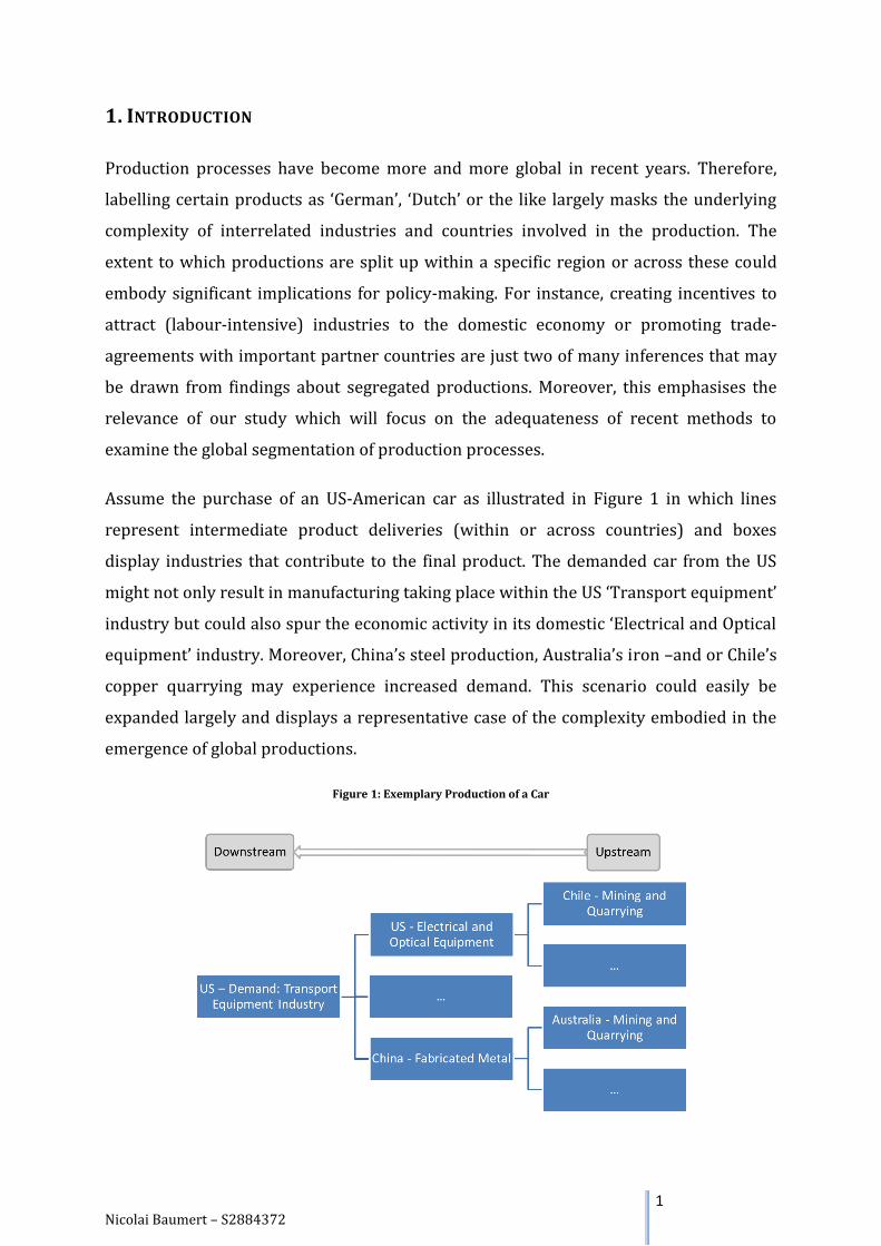
Assume the purchase of an US-American car as illustrated in Figure 1 in which lines
represent intermediate product deliveries (within or across countries) and boxes
display industries that contribute to the final product. The demanded car from the US
might not only result in manufacturing taking place within the US ‘Transport equipment’
industry but could also spur the economic activity in its domestic ‘Electrical and Optical
equipment’ industry. Moreover, China’s steel production, Australia’s iron –and or Chile’s
copper quarrying may experience increased demand. This scenario could easily be
expanded largely and displays a representative case of the complexity embodied in the
emergence of global productions.
Figure 1: Exemplary Production of a Car

Nicolai Baumert – S2884372
2
It also introduces the term fragmentation as the production is split up into different
parts realized by various industries and countries. Therefore, fragmentation is defined
as the disintegration of production structures across and within national boundaries
(López-Gonzalez, 2012). To entitle the emergence of scenarios similar to Figure 1,
Gereffi (1989) stated that: ‘The Global Factory is on the rise’1 describing the variety of
countries involved in the production of single products and therefore combined under
one figurative (factory) roof. Few scholars would disagree with this metaphorical
assertion since shrinking transaction costs of trade have certainly contributed to more
interdependent global markets with extensive cross-country trade.
In this paper, we will therefore assess the reliability of recent studies which examine the
extent to which the involved countries in globally fragmented production processes
contribute to the final product value (e.g. Los et al, 2015). This will be relevant as we
already established that policy-makers are well-advised to consider trends in global
production fragmentations in their decisions.
The extensive international fragmentation of production has been observed in several
case studies decomposing production processes into multiple global production stages
such as Dedrick et al. (2009) and Dudenhöffer (2005). Moreover, this calls for measures
which could expand the phenomenon to a macroeconomic perspective. However,
traditional concepts of national competitiveness based on comparisons of gross export
statistics are not suitable to account for emerging global intermediate good trade
anymore (Koopman, 2014). These always capture the full border-crossing product value
instead of the actual contribution of the exporting country and inflate trade statistics
relative to the final good value2. Thus, Timmer et al. (2013) propose a different
definition of competitiveness as the ‘ability to perform activities meeting the test of
international competition and generate increased income and employment’.
Furthermore, the value added (VA) – defined as the contribution of an industry to the
overall value of a product – and its fragmentation is misrepresented for the most part
when consulting gross export figures (and ratios).
1 Grunwald & Flamm (1985) and Buckley & Ghauri (2004) offered related but different term interpretations
2 In Figure 1, this would imply that the entire product value of China’s ‘Fabricated Metals’ delivery to the US-American
car production is measured. This not only includes actual Chinese contributions but also Australia’s ‘Mining and Quarrying’ deliveries at an earlier production stage.

Nicolai Baumert – S2884372
3
Therefore, many studies that examine global production fragmentation are increasingly
based on the concept of input-output (IO) analysis. By explicitly distinguishing between
inter-industry deliveries of intermediate goods (in the so-called intermediate matrix)
and the supply of finished goods to a final demand (FD) category (in the FD matrix), IO
analysis is able to identify each industry’s contributed VA for the related production
stage. Consequently, it traces the factor inputs needed in order to produce a final good
and comprehensively computes the overall VA by involved industries embodied in an
industry’s output (Timmer et al., 2014). In addition, matrix algebra allows the analyses
to capture direct but also indirect VA requirements arising for the respective industries3.
Due to improved data availability, IO analysis nowadays allows for conclusions about
complex international production networks. All the more important, this paper will
attempt to judge the reliability of global fragmentation studies employing these IO
concepts (e.g. Los et al., 2015) by analysing potential biases embodied in these papers.
This necessary research area remained rather unexplored until now4 and is where this
paper fills in by testing for the magnitude of potential biases found by Nomaler &
Verspagen (2014) (N&V). These may distort IO analyses about global production
fragmentation which are based on the aggregation of multiple different individual
production processes within industries at different stages of the overall production. In
turn, the aggregation comes up since – other than in the aforementioned case studies by
Dedrick et al. (2009) or Dudenhöffer (2005) – broader macroeconomic studies tend to
pool multiple different final products together.
Our analytical approach employs simulation results that are – different from N&V’s
(2014) analysis – based on empirical data for various industrial aggregation levels. We
thereby examine the empirical scope of the biases with the research question:
Do the biases identified by Nomaler & Verspagen (2014) significantly distort the empirical
findings of studies examining the value added distribution in globally fragmented
production processes if input-output analysis is employed?
3 This would for instance imply that Figure 1’s ‘Mining industry’ of Chile also requires ‘Electrical and optical
equipment’ from the US for the quarrying. The production of a car in the US would not only rely on ‘Electrical and optical equipment’s direct VA but also on the value that it supplies to ‘Mining’ in Chile at an earlier stage 4 A mentionable contribution in this field is Baldwin & López-Gonzales (2015) focusing on data constrains and
insufficient consideration of firm heterogeneity.

Nicolai Baumert – S2884372
4
The remainder of this paper is organised as follows: Chapter 2 provides the reader with
a brief overview of the emergence of IO analysis in general, the basic concept underlying
it, most important literature contributions studying global fragmentation of production
and its recent criticism. Chapter 3 presents the investigated biases in more detail before
Chapter 4 focuses on the employed data and its processing. Subsequently, Chapter 5
analyses the data and presents the simulation approach. Chapter 6 documents and
illustrates the empirical results. Moreover, it indicates the implications of the findings
for recent indicators measuring the value added distribution in globally fragmented
production processes. Then, Chapter 7 concludes the paper by summarizing the results
and identifying limitations of the paper as well as suggestions for future research.
2. LITERATURE REVIEW
Decreasing costs for communication as well as the coordination of trade have led to
enormous international fragmentation of economic activity. Consequently, production
largely shifted from the national towards the international scope. Thus, value chains –
the whole range of economic activities required to complete a final good – have become
increasingly global (Gereffi, 1999).
2.1. GLOBAL PRODUCTION FRAGMENTATION
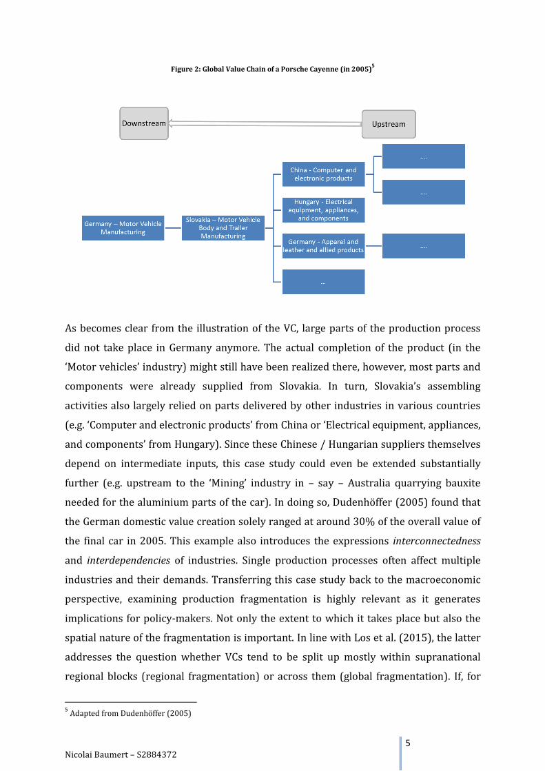
By illustrating this claim based on an exemplary product, Dudenhöffer (2005)‘s much-
cited study of the global value chain (VC) of the luxurious German car ‘Porsche Cayenne’
has received much attention. Within the study, the author identified the VA which was
actually generated within Porsche’s domestic market (i.e. Germany) in 2005. The
Porsche Cayenne completed (and sold) in Germany was examined with regards to the
suppliers of the finalising firm (i.e. Porsche). These, however, in turn relied on other –
more upstream – component delivering companies themselves. Part of the related VC is
depicted in Figure 2.
Nicolai Baumert – S2884372
5
Figure 2: Global Value Chain of a Porsche Cayenne (in 2005)5
As becomes clear from the illustration of the VC, large parts of the production process
did not take place in Germany anymore. The actual completion of the product (in the
‘Motor vehicles’ industry) might still have been realized there, however, most parts and
components were already supplied from Slovakia. In turn, Slovakia’s assembling
activities also largely relied on parts delivered by other industries in various countries
(e.g. ‘Computer and electronic products’ from China or ‘Electrical equipment, appliances,
and components’ from Hungary). Since these Chinese / Hungarian suppliers themselves
depend on intermediate inputs, this case study could even be extended substantially
further (e.g. upstream to the ‘Mining’ industry in – say – Australia quarrying bauxite
needed for the aluminium parts of the car). In doing so, Dudenhöffer (2005) found that
the German domestic value creation solely ranged at around 30% of the overall value of
the final car in 2005. This example also introduces the expressions interconnectedness
and interdependencies of industries. Single production processes often affect multiple
industries and their demands. Transferring this case study back to the macroeconomic
perspective, examining production fragmentation is highly relevant as it generates
implications for policy-makers. Not only the extent to which it takes place but also the
spatial nature of the fragmentation is important. In line with Los et al. (2015), the latter
addresses the question whether VCs tend to be split up mostly within supranational
regional blocks (regional fragmentation) or across them (global fragmentation). If, for
5 Adapted from Dudenhöffer (2005)

Nicolai Baumert – S2884372
6
instance, Los et al. (2015) detect the global fragmentation of VCs to grow distinctly more
rapid than the regional fragmentation, the consequences for policy-makers might clearly
diverge. Sticking with the example, strong regional fragmentation could call for regional
trade agreements whereas more intense growth of global fragmentation might require
multiregional trade policies. Due to the necessity to study these phenomena, IO analysis
has evolved to an important tool for economic analysis. Broadly considered as an
adequate approach to reflect complex international interconnectedness which enables
the derivation of policy implications, IO analysis’ increasing usage obviously depends on
its reliability. This fuels the topicality of this paper as we will empirically test the
significance of potential distortions in the methodology of IO concepts used to examine
the VA distribution within globally fragmented VCs.
2.2. INTRODUCTION TO INPUT-OUTPUT ANALYSIS
VCs are often illustrated as a linear sequence which starts off with the chronologically
first involved industry (the most upstream industry in the production of a final good).
From there onwards, the product value is complemented by the second (more
downstream) industry and so forth until the final product is ultimately consumed. A
simple example of such a VC is shown in Figure 36.
Figure 3: General Model of linear Value Chain
6 Akin to Timmer et al. (2013). Unlike in the figures before boxes represent either industries or FD categories.
Industry 2, 4 and 6 will be added at a later stage when introducing multiple VCs.

Nicolai Baumert – S2884372
7
Figure 3’s can be interpreted as follows. Three different industries across different
countries represent the VC which generates the final product consumed by FD. Industry
1 forms the most upstream value adding stage in the VC which delivers its intermediate
good valued at 5 $ to industry 3. In turn, industry 3 contributes an additional 10 $ worth
of product value to the good which sums up to 15 $ of total product value. The same
logic applies for the final 10 $ of VA contributed by the most downstream industry 5
amounting to 25 $ of total product value. Here, the product is finalised before being
ultimately consumed by the FD category. As observable, the product value within this VC
gradually increases as value is added to the product at every VC stage. Consequently, the
final product value amounts to the sum of all VA contributions. A VC as in Figure 3 is
referred to as linear since the output of each VC stage is fully delivered to the ensuing
stage and only one sequential path of deliveries is possible (i.e. from Industry 1 to 3 to 5
before the completed product is consumed by the FD).
Several studies examining production fragmentation have been realized in recent years.
Apart from the aforementioned study by Dudenhöffer (2005), for instance, Dedrick et al.
(2009) employed the iPod as an exemplary product to describe the extensive global
production fragmentation of modern VCs. Nevertheless, these microeconomic literature
contributions examining production fragmentation were only based on specific product
case studies (i.e. the Porsche Cayenne or the iPod). Consequently, broader measures
which allowed for generalizations about the fragmentation of VCs on a national, regional
and global scale were needed to be able to derive policy implications which would
address the related overall economy trends. Moreover, the aforementioned surge of
global VCs also challenged the suitability of traditional economic indicators based on
gross exports to adequately reflect the contributions of the involved industries and
countries to the production processes. Building on earlier pioneer work by Hummels et
al. (2001), contributions by Koopman et al. (2014) and Wang et al (2014) documented
the so-called ‘double-counting’ problem causing gross exports to inadequately account
for intermediate trade. This issue is relevant for our paper since it forms a major part of
the reasons why IO models have increasingly become popular for global production
fragmentation studies. This emphasises the importance of our study which examines the
suitability of IO models to analyse the distribution of VA in fragmented VCs.
To illustrate the principles of ‘double-counting’ with the help of Figure 3, suppose that
Industry 1 and 3 as well as the consumption by the FD are located in a given country A

Nicolai Baumert – S2884372
8
whereas Industry 5 is situated in country B. Consequently, the VA contributed to the VC
by country A amounts to 15$ while country B only adds 10$ to the final product value.
However, this set-up yields significant differences between the actual VA generated
within the countries and their gross exports as indicated in trade statistics. Although
country A contributes more value to the production process, its gross exports (15 $) are
lower than country B’s (25 $). Therefore, not only does both countries’ total sum of gross
export value (40 $) exceed the final product value of the consumed good but the
difference between gross exports and VA within a country is also mostly not
proportionate. In other words, even if a country contributes significantly more to a
global VC than another one, its gross export value might be drastically below its trade
partner depending on the realized VC stages and their order. Consequently, the
meaningfulness of gross trade statistics to adequately represent competitiveness has
decreased largely with intensified fragmentation. This links the ‘double-counting’ to our
study. Since IO analysis is able to avoid the illustrated problem while accounting for
inter-industry and global interconnectedness, it has recently gained more attention by
numerous economic scholars. Moreover, its improved data availability facilitated the use
and allows for generalisations about fragmentation instead of limiting insights to case
studies like the ones by Dudenhöffer (2005) and Dedrick et al. (2009). Therefore, it will
be important to judge the reliability of IO concepts to reflect production fragmentation.
In principle, the concept underlying the usage of IO data for economic analyses is rather
straight-forward. The data comprised by national input-output tables (NIOTs) is
typically gathered by the country’s statistical institutions on a regular (mostly yearly)
basis (Timmer et al., 2015). The structure of a NIOT is illustrated in Table 17.
Table 1: Structure of a National Input-Output Table
Within this framework, the broad distinction is between an industry’s supply (rows) and
an industry’s use as well as final consumption (as columns) of the delivered goods.
7 Adapted from Timmer et al. (2015)
Industry 1 Industry 2 … Industry S Final Use 1 … Final Use K
Industry 1
Industry 2
…
Industry S
Total
Output
Co
un
try
N -
Sup
ply
Value Added
Gross Output
Country N - Intermediate Uses Country N - Final Use

Nicolai Baumert – S2884372
9
Hence, columns depict the required intermediate good deliveries for the production by
one respective industry (e.g. coal mining) or the supply of completed products for the
consumption by one final use category (e.g. private household consumption). These
columns are displayed as vertically (intermediate matrix) and horizontally striped (FD
matrix) respectively. Moreover, each industry’s particular VA for the regarded
timeframe (mostly one year) is added below its intermediate good consumption in the
VA row vector which sums up to the overall gross output of the respective industry. On
the other hand, the rows of the NIOT generally indicate the value of the deliveries and
output generated by the related industries. More specifically, in a NIOT with s = 1,…, S
industries the intermediate matrix Z contains S x S cells with intermediate deliveries.
Each respective cell zi j therefore describes how much product value industry i delivers
to industry j. On the other hand, the final demand matrix F consists of S x K cells where k
= 1, …, K denotes the number of FD categories . Furthermore, the VA vector w’ (where a
prime denotes a transposed vector) contains all 1 x S value added elements wj’ where j
refers to the value generating industry. The summation of each row therefore yields the
related industry’s gross output embodied in the S x 1 vector x and its counterpart x’
(Dietzenbacher et al., 2013). Extending this structure to an international dimension,
global input-output tables yield a scheme following the logic illustrated in Table 28. This
expanded framework lists the deliveries (incl. imports) of intermediate inputs and final
goods from all countries in the table’s rows. Similarly, industries and FD categories are
include all country-industry (e.g. Transport equipment in Germany) or country-FD
category (e.g. Dutch Personal consumption expenditure) combinations.
Table 2: Structure of a global Input-Output Table
8 Adapted from Timmer et al. (2015)
Industry 1 … Industry S … … Industry 1 … Industry S FU 1 … FU K … … FU 1 … FU K
Industry 1
…
Industry S
…
…
Industry 1
…
Industry S
Total
Output
Co
un
try
N
- Su
pp
ly
Value Added
Gross Output
Country N - Uses Country N - FU…Country 1 - Uses
Co
un
try
1
- Su
pp
ly…
Country 1 - Final Use (FU) …

Nicolai Baumert – S2884372
10
Consequently, the deliveries to a country’s industry or FD category are shown in the
vertically (country-industry) and horizontally striped (country-FD category) columns.
Since the IO data availability is mostly limited to developed countries, the remainder is
summed to a ‘Rest-of-World’ category (as country N). Assuming n = 1,…, N countries, this
results in the extension of the intermediate matrix Z to its new dimensions of SN x SN
cells whereas the FD matrix F now contains SN x NK elements. Similarly, w’ is expanded
to 1 x SN cells and x now contains SN x 1 elements (Los et al., 2015).
2.3. PRACTICAL USE OF INPUT-OUTPUT TABLES IN VALUE CHAIN ANALYSIS
In order to establish an understanding of the logic underlying the use of IO tables, Table
3 translates the linear VC given in Figure 3 into a NIOT.
Table 3: Translation of linear VC into National Input-Output Table
In line with the earlier and more general descriptions of IO tables in Table 1 and 2, this
table can be interpreted as follows. Since the rows and columns of the square (6-by-6
industries) matrix denoted with ‘Intermediate Uses’ show the deliveries from the row
industry to the column industry which contains the respective cell, it is clearly
observable that Industry 1 (first row) delivers 5 $ to industry 3 (third column). Since
this forms the first delivery of the VC, the VA by industry 1 equals the value of the
delivery (5 $). A similar logic applies to the delivery of 15 $ in product value from
industry 3 (third row) to industry 5 (fifth column). However, as industry 1 had already
contributed a VA of 5 $ in VC stage 1, the added value by industry 3 only amounts to 10 $
(15 $ product value minus 5 $ intermediate good demand). Finally, industry 5 delivers
the finished product to the Final Use category which also marks the stage in which the
Intermediate matrix and thereby the VC is left. Since the previous product value already
summed up to 15 $ whereas industry 5 delivers 25 $ to the FD, the last VA contribution
by industry 5 can be computed as 10 $. In this simple example (which will later be
Country N -Final Use
Industry 1 Industry 2 Industry 3 Industry 4 Industry 5 Industry 6 Final Use
Industry 1 0 0 5 0 0 0 0 5
Industry 2 0 0 0 0 0 0 0 0
Industry 3 0 0 0 0 15 0 0 15
Industry 4 0 0 0 0 0 0 0 0
Industry 5 0 0 0 0 0 0 25 25
Industry 6 0 0 0 0 0 0 0 0
5 0 10 0 10 0
5 0 15 0 25 0
Total
Output
Co
un
try
N -
Su
pp
ly
Value Added
Gross Output
Country N - Intermediate Uses

Nicolai Baumert – S2884372
11
expanded), industry 2, 4 and 6 do not take part in the VC. Following from the double-
entry bookkeeping principle is the IO tables’ characteristic of each industry’s gross
output being equal to the sum of all demands (as intermediate or final good) served by
the same industry. With this in mind, the introduction of coefficients is in order. These do
not form part of the general IO table but can be derived from it and are indispensable for
the calculations at a later stage. For instance, the elements ai j of the input coefficient
matrix A with the dimensions SN x SN describe how much output a given industry i (as
the row of the intermediate matrix) directly delivers to industry j (as the column of the
intermediate matrix) in order to produce one additional unit of output in industry j. For
a35, industry 3’s deliveries to industry 5, this would yield 0.6 using
ai j = zi j / xj . (1)
A similar logic applies to the derivation of the VA coefficient vector p’ with its elements
pj. These coefficients are understood as the shares of a (column) industry’s VA in the
output value of one unit generated in that industry. In other words, a VA coefficient
indicates how much VA a given industry j directly generates in order to produce one unit
of its output. For instance, p5 yields 0.4 when employing
pj = wj / xj (2)
Moreover, simple matrix algebra enables IO analysis to account for direct and also
indirect product requirements (recall Figure 6) drawing on the so-called Leontief inverse
matrix M. Consequently, its elements mi j embody the required production levels of each
separate industry i necessary to generate one unit of (additional) FD for industry j.
Therefore, a single element of the inverse matrix is interpreted as the extra output
necessary from industry i to produce one unit of output in industry j. The derivation of
the matrix is slightly more complicated although the intuition behind it is rather
straight-forward as well. Recall that the input coefficient matrix A incorporates elements
indicating the output of an industry i directly necessary to produce a unit of output in
industry j. Based thereupon, we multiply A with the final demand vector fi which
includes one unit of demand in industry i and zeros for all remaining elements. In
mathematical terms this yields Afi which equals the direct production requirements of
all industries to generate fi. However, in order to produce Afi, additional output is

Nicolai Baumert – S2884372
12
required once more equalling Afi * A = A2 * fi and so forth. Finally, the sum of this
geometric series yields the general form of the Leontief inverse given by
M = (I - A) -1 (3)
where I denotes the identity matrix with ones on the diagonal and zeros elsewhere.
Consequently, multiplying with M accounts for not only the direct output requirements
(as in A) but also the indirect output necessities. This also enables the calculation of the
gross output vector x (SN x 1) from the FD vector f (SN x 1) using
x = Mf (4)
which allows for the more thorough examination of scenarios like in Figure 1. Provided
this structure and sufficient data availability, IO models can be an important tool used to
examine demand-driven interdependencies of industries on a national as well as on a
regional or global scale. Moreover, the problem of ‘double-counting’ as introduced above
is avoided since the focal point of the analysis is the VA rather than the gross exports.
This has led to increased prominence of the models in economic analyses. Therefore, the
aim of our paper to evaluate the reliability of findings about the VA distribution in the
course of global production fragmentation based on IO analysis is of high importance.
2.4. RELEVANT PRIOR STUDIES
Before, however, we will briefly introduce recent studies including measurements of
(national) competitiveness, vertical specialisation and regional fragmentation9. These
will be relevant as they not only help to distinguish which of the IO-based concepts are
subject to criticism but also since they build up on each other, subsequently leading
towards this paper’s subject of investigation: the potential distortion of global
production fragmentation studies quantifying the VA distribution. Three similar yet
different approaches of studying global VCs can be distinguished.
First, Hummels et al. (2001) developed the concept of vertical specialisation. Thus, the
degree of vertical specialisation was defined as the share of imported inputs embodied
9 Vertical specialisation is defined below; exemplary contributions studying its concept include Hummels et al. (2001)
and Amador & Cabral (2009). Regional fragmentation receives attention in e.g López-Gonzales (2012), Baldwin & López‐Gonzalez (2015), and Los et al. (2015) as well as implicitly in Johnson & Noguera (2012b)

Nicolai Baumert – S2884372
13
in the total exports to the directly subsequent countries10. Consequently, the focus of
their study was shifted from traditional trade in final products towards modern trade in
intermediate goods to account for the increased fragmentation of production processes.
Thereby, Hummels et al. not only considered direct imports embodied in the exports of a
given country but also its indirectly imported goods which are contributed to the
country’s exports. The study finds that vertical specialisation grew by 28 percent up to
21 percent between 1970 and 1990 for ten member countries of the Organisation for
Economic Co-Operation and Development (OECD) and four emerging countries. Limited
to NIOTs, the model did not account for ‘back-and-forth trade’ where exports of a
country eventually get imported again. Only deliveries directly received from or
supplied to foreign countries were regarded. However, the study already emphasised
the recently increased extent of production fragmentation while relying on IO models.
A decade later, Johnson & Noguera (2012a) introduced the value-added-to-gross export
ratio (VAX ratio). The VAX ratio is defined as the VA of a country that is eventually
consumed as part of FDs in all foreign countries as a ratio of total export value. Thereby,
Hummels et al.’s focus on the importing country was shifted towards the country in
which the final demand for a product is located. Referring back to Figure 3 and assuming
all trade to be international, Hummels et al.’s approach would aim to quantify industry
3’s import share embodied in its exports to industry 5. In contrast, the VAX ratio would
intent to compute how much VA generated in industry 3 would ultimately be consumed
elsewhere. Among their findings, Johnson & Noguera (2012a) concluded that VAX ratios
vary largely across countries and industries and that the differences between VA and
gross trade are strong (VAX ratio mostly far below 1). Again, these findings shed light on
the importance of fragmentation studies that this paper will test for their reliability.
Third and last, Timmer et al. (2013) established the ‘Global Value Chain (GVC)
approach’. As the term implies, the focal point of this concept is rather one specific
global VC and, therefore, the last value adding country before consumption (country-of-
completion). The location of the FD is irrelevant. Timmer et al. (2013) therewith also
developed to the indicator ‘GVC income’ which is represented in Figure 411.
10
Thereby, Feenstra & Hanson (1999) is extended where offshoring as the share of imported intermediates inputs in total intermediates inputs is measured 11
Adapted from Los (2016)

Nicolai Baumert – S2884372
14
Figure 4: Global Value Chain Income of Country 2
The GVC income describes the VA that a country (here Country 2) contributes to the
final output of one specific VC (completed in Country 3). Therefore, all output by
Country 3 (in black) – to serve FDs in Country 3 and 5 – is considered for this concept.
However, only parts of Country 2’s output are incorporated in Country 3’s output since
Country 2 serves other FDs, as well. Consequently, to calculate Country 2’s GVC income
for Country 3’s output, only the VA which Country 2 contributes to Country 3 is
considered. For instance, Timmer et al. (2013) decompose the output of final goods from
the German ‘Transport equipment’ industry into the GVC income shares of the domestic
country and foreign contributions by dividing the respective VA by the overall FD of
‘Transport equipment’. Consequently, the GVC income regards one specific VC and
examines the involved countries’ contribution to it. Based on this approach, Los et al.
(2015) distinguish between the domestic, regional and global VA and thereby dived
even further into the GVC and its spatial characteristics. They challenged Baldwin &
López-Gonzales’ (2015) hypothesis that VC trade is still regional and mostly takes place
within trade blocks (e.g. the European Union (EU) or the North American Free Trade
Organisation (NAFTA)). However, Baldwin & López-Gonzales’ (2015) arguments were
based on a gross exports perspective. As shown by Los et al. (2015), employing VA
instead of gross exports yields different results (recall Chapter 2.2.). Los et al. (2015)
forms a major part of this study as it focuses on specific VCs and the examination of their
characteristics in terms of the VA distribution. Since this paper seeks to quantify the
extent to which such studies may be biased we will refer back to it at a later stage and
attempt to quantify its potential distortion. More specifically and in line with Timmer et
al.’s (2013) measurement, Los et al. (2015) decompose the value of final products –

Nicolai Baumert – S2884372
15
defined by the last contributing country in a VC (i.e. the country-of-completion) – into
the value contributed by all involved countries, respectively. Consequently, they first
sum all FDs for a product i in a country n over its various final use categories (e.g.
household expenditure or government consumption). This summation arises from the
multiplication of the FD matrix F with a summation vector e (consisting of ones) and is
thereby realized for all industries domestically and abroad. It yields a SN x 1 vector f
which displays all total FDs for each product i. These elements shall be decomposed into
all industries’ respective (direct and indirect) VA distribution. In order to do so, the VA
coefficients need to be enriched by their indirect components. Therefore, a matrix p
containing the VA coefficients pj on the diagonal and zeros elsewhere is created. When
this matrix p is subsequently multiplied with the Leontief inverse matrix M as in
equation (1), its VA coefficient elements are increased by their indirect contribution
share (through element-wise multiplication with the M’s diagonal values). Therefore, by
employing the M’s capability to account for indirect industry contributions we ensure
that all embodied VA requirements are considered in the subsequent computation of VA
distributions. As Los et al. (2015) aim to compute how much VA of the FD for one VC is
attributable to each industry (domestic or foreign) separately, pM is multiplied by a SN x
1 vector fi only containing the FD element for product i and zeros elsewhere. This yields
v = pM fi (5)
where v is a SN x 1 vector in which each cell indicates the VA contribution to the final
value of product i directly and indirectly incorporated by the respective industry. A
summation of this vector would logically amount to product i’s overall value of FDs.
Following this, the summation of all VA elements vi which are generated outside of the
country-of-completion of the product i are considered as foreign VA. Dividing this
foreign contribution by the overall final product demand for product i therefore yields
the foreign value added share (FVAS) as the VA contributions generated outside of the
country-of-completion as a share of the industry’s final output. Thereby, it is
distinguished from the domestic value added share complementing the FVAS to 1. This
indicator’s distortion will be examined by realising simulations at a later stage.
Subsequently, Los et al. (2015) are able to disaggregate the FVAS further by
differentiating between regional and global FVASs. They argue that although regional
fragmentation is still dominant, the global fragmentation share grew substantially faster

Nicolai Baumert – S2884372
16
recently. This development of a new ‘Factory World’12 has only briefly been suspended
during the financial crisis of 2008 and regained strength afterwards again. Despite the
fact that we will naturally not be able to test the distortion of regional compared to
global foreign value added shares within the scope of this paper since we are limited to
national data, the principles underlying the biases also apply for these more specific
spatial dimensions of value added shares.
2.5. RESEARCH GAP
The aforementioned studies were largely enabled and facilitated by the improved
availability of global IO data (e.g. the OECD – World Trade Organisation (WTO) Trade in
Value Added Database13 or the World Input-Output Database (WIOD))14. Therefore and
as elaborated upon above, IO analysis has become an important tool to examine global
production fragmentation. Consequently, it is important to be able to judge the
reliability of the model’s findings regarding the VA distribution in global production
fragmentation studies which will form the focal point of this paper. Only if it is possible
to verify the reliability of the model or at least quantify potential biases in these studies,
will results and the subsequent interpretations of them be generalizable.
In order to challenge the meaningfulness of IO analyses investigating the VA
distributions within VCs, N&V (2014) use the study by Los et al. (2015) as an initial
point to examine potential biases in the employed model. They analyse the IO model
theoretically and run simulations identifying biases which are based on the fact that IO
analysis assumes that each industry only produces one good whereas in reality this
clearly does not hold. If multiple VCs are aggregated and thereby result in the
occurrence of one single industry at multiple stages within one VC, the degree to which
its contributions are up or downstream might differ largely. This may distort the validity
of findings derived from IO analysis attempting to measure the industries’ VA
contribution to single VCs significantly. According to N&V (2014), the VA generated by
the final industry may be overstated which would result in an overestimated VA
contribution by the respective country-of-completion. Nevertheless, they also consider
scenarios in which the contribution of the final industries will be underestimated if
these add a large amount of VA to the VC. 12
A term akin to the aforementioned ’Global Factory’ allegory by Gereffi (1989) 13
OECD-WTO (2012) 14
Timmer et al. (2015)

Nicolai Baumert – S2884372
17
However, so far no empirical quantification of the distortions that the VA distribution is
subject to has been done. This is where our paper fills in to close the research gap. In
order to do so, this study will simulate concepts introduced by Los et al. (2015) with
actual empirical data. As we will obtain and employ the same dataset on various
aggregation levels and since N&V’s (2014) biases are also based on aggregation,
differing results of our simulations will yield inferences on the extent to which global
fragmentation studies’ findings about VA distributions along the VC are distorted.
3. THE BIASES IDENTIFIED BY NOMALER & VERSPAGEN (2014)
At this stage and before diving into the explanations of the specific biases by N&V
(2014), it is worth to briefly outline the structure of the remainder of this paper. First,
the biases which have been identified by N&V (2014) based on the aggregation of
multiple individual VCs to a limited number of indicated sets of these in IO databases
will be explained and illustrated in more detail. Second, US-American data about inter-
industry deliveries as well as FD categories within the country is gathered on which the
subsequent simulations will be based. Since the tables rely on the same data but contain
information for three different aggregation levels (hence: differing numbers of listed
industries) per year, comparisons of the simulation results across this data will shed
light on the extent to which aggregation leads to distortion. Consequently, we will
convert the data into IO tables like illustrated in Table 3 and compare the results for
indicators that measure the VA distribution across the various aggregation levels.
Moreover, the emerging NIOTs will be transformed into hypothetical global IO tables
since we are interested in the magnitude to which international VCs might be distorted.
Multiple scenarios with an adjustable number of countries as well as different degrees of
international trade will be developed to enable generalisations about the extent of the
biases under various circumstances (i.e. high or low internationalisation; many or few
countries). Although these global tables will be hypothetical, they are assumed to
describe realistic VCs quite accurately since the data that is being employed is based on
empirical data which distinguishes it from the VCs that were used by N&V (2014) to
identify the biases. This will enable us to expand the distortions’ examination
empirically. Third, these different scenarios – with varying number of countries and
degrees of international trade – are used to simulate a recent measurement of the VA

Nicolai Baumert – S2884372
18
distribution in the course of global production fragmentation (i.e. the FVAS, recall
Chapter 2.4.). The results of these simulations can then be compared across the different
obtained aggregation levels. As explained in more detail in this chapter, N&V’s (2014)
errors are based on the aggregation of single VCs into a limited number of bundled VCs.
Therefore, the discrepancy of the results for the VA distribution in globally fragmented
productions between the aggregation levels indicates the level of distortion which may
be caused by these errors. Thus, it will be possible to quantify the extent to which N&V’s
(2014) biases distort studies on VA distribution using IO analysis. Forth, the
discrepancies across the results derived from the tables which differ in their aggregation
extent will be analysed and interpreted. Consequently, the reliability of IO models for
global fragmentation studies and their findings with regards to the distribution of VA
will be assessed based on the simulation results.
With that in mind, it is crucial to establish a clear and comprehensive understanding of
the nature of N&V’s (2014) criticism in more depth. Only if the underlying concepts of
the errors are grasped, they can be related to the suitability of IO models for studies
examining the international segmentation of VCs. When using IO analysis to examine
global production fragmentation, the aggregation of all VCs that an industry (e.g.
‘Manufacturing’) adds value to, might not represent the individual contributions (e.g. to
‘Machinery Manufacturing’ or to ‘Electronic Product Manufacturing’) accurately. For
instance, the results for the FVAS (Los et al., 2015), might misrepresent the real VA
contributed to single VCs. Recall Table 3 as our example of a linear VC translated into an
IO table. Moreover, we transfer the example to a more illustrative case assuming that
industry 1 constitutes ‘Copper mining’, industry 3 represents ‘Electronical components’
and industry 5 shows ‘Transport equipment’. ‘Personal consumption expenditures’ is the
only FD category and the VC’s final product may be a car. Intermediate deliveries from
the ‘Copper mining’ industry (e.g. used to produce wires or cables) are required to
produce the car’s automobile radio in the ‘Electronic components’ industry before the
‘Transport equipment’ industry implements this radio to finish off the final car and
deliver it to the FD. Therefore, it is the only industry supplying goods to the FD. Figure
615 translates the case into an IO following the logic introduced in Chapter 2.3.
15
Adapted from Timmer et al. (2015)

Nicolai Baumert – S2884372
19
Table 4: Translation of linear Transport Equipment Value Chain into an Input-Output Table
Now, suppose that another production process takes place within the same economy.
Within this second VC, industry 2 represents ‘Lithium mining’, industry 4 constitutes
‘Electrical parts’ and industry 6 indicates ‘Telecommunication equipment’. The final
product – a mobile phone which needs inputs from the ‘Lithium mining’ industry before
‘Electrical parts’ manufactures a battery for the phone – is completed in
‘Telecommunication equipment’. Then, we translate the VC in which only
‘Telecommunication equipment’ supplies the FD, into the previous Table 4 and therewith
combine it with the first VC. This yields our new combined Table 516.
Table 5: Input-Output Table including two Value Chains
As observable in the table, all individual VC contributions (e.g. ‘Copper mining’ supplying
5 $ to ‘Electronic components’) as well as the respective VA coefficients (e.g. p4 = 0.5) are
clearly observable from the table (recall equation (2)). Now, by using matrix algebra we
16
Adapted from Timmer et al. (2013)
Final Use
Copper
mining
Industry
2
Electronic
components Industry 4
Transport
Equipment Industry 6
Personal
consumption
expenditures
Copper mining 0 0 5 0 0 0 0 5
Industry 2 0 0 0 0 0 0 0 0
Electronic
components 0 0 0 0 15 0 0 15
Industry 4 0 0 0 0 0 0 0 0
Transport
Equipment 0 0 0 0 0 0 25 25
Industry 6 0 0 0 0 0 0 0 0
5 0 10 0 10 0
5 0 15 0 25 0
Total
Output
Co
un
try
N -
Su
pp
ly
Value Added
Gross Output
Country N - Intermediate Uses
Final Use
Copper
mining
Lithium
mining
Electronic
components
Electrical
parts
Transport
Equipment
Tele-
communication
equipment
Personal
consumption
expenditures
Copper mining 0 0 5 0 0 0 0 5
Lithium mining 0 0 0 10 0 0 0 10Electronic
components 0 0 0 0 15 0 0 15
Electrical parts 0 0 0 0 0 20 0 20
Transport
Equipment 0 0 0 0 0 0 25 25
Tele-
communication
equipment 0 0 0 0 0 0 25 25
5 10 10 10 10 5
5 10 15 20 25 25
Country N - Intermediate Uses
Total
Output
Co
un
try
N -
Su
pp
ly
Value Added
Gross Output

Nicolai Baumert – S2884372
20
will be able to compute each industry’s VA contribution to a given VC. For exemplary
purposes, we will only regard the final demand f5 of 25 $for the ‘Transport Equipment’
industry. The remaining cells of the 6 x 1 vector contain zero-values. Using equation (3)
and (4) we can now generate the output level only associated to the FD for cars. To
generate the new VA levels necessary to serve the FD, we employ equation (5) yielding a
6 x 1 vector v with the VA levels of all respective industries. Since the industries are not
interrelated at the disaggregated level, the computations yield the indicated VA (i.e. 5, 10
and 10 $) for industry 1, 3 and 5 from Table 5. Consequently, the IO-based VA
calculation reflects the actual contributions of each industry to the VC of ‘Transport
equipment’. As mentioned before, however, N&V (2014) base their critic on the
aggregation of multiple individual VCs into an aggregated set of VCs industry. Hence,
suppose that the ‘Electronic components’ industry is bundled together with the
‘Electrical parts’ industry to a new overarching industry called ‘Electrical and electronic
components’. The emerging IO table now looks slightly different as shown in Table 6.
Table 6: Aggregated IO Table including two Value Chains17
This leads to the fact that individual VC contributions of the former industries ‘Electronic
components’ and ‘Electrical parts’ are no longer observable. Consequently, again
employing equation (2) now yields a VA coefficient p3 for both included industries in
‘Electrical and electronic components and parts’ at 0.57 compared to 0.5 for ‘Electrical
parts’ and 0.67 for ‘Electronic components’ before.
The difference is due to the fact that less value had already been added to the first VC (5
$) prior to ‘Electronic component’s contribution to it when compared to the second VC
17
Adapted from Timmer et al. (2013)
Final Use
Copper
mining
Lithium
mining
Electrical and
electronic
components
Transport
Equipment
Tele-
communication
equipment
Personal
consumption
expenditures
Copper mining 0 0 5 0 0 0 15
Lithium mining 0 0 10 0 0 0 10
Electrical and
electronic
components 0 0 0 15 20 0 35
Transport
Equipment 0 0 0 0 0 25 25Telecommunication
equipment 0 0 0 0 0 25 25
5 10 20 10 5
5 10 35 25 25
Country N - Intermediate Uses
Total
Output
Co
un
try
N -
Su
pp
ly
Value Added
Gross Output

Nicolai Baumert – S2884372
21
in which the product value prior to the ‘Electrical parts’ contribution was already higher
(10 $). Value that is added when the relative product value is already higher is termed as
more downstream whereas the contribution at a stage when the product value is still
relatively low is considered more upstream in the VC. Thus, comparing the aggregated
VA coefficients with the disaggregated ones, it becomes clear that the VA coefficients of
the more downstream contribution (i.e. Electrical parts’) is overestimated (0.57 versus
0.5) whereas the more upstream value addition (i.e. Electronic components’) is
underestimated (0.57 versus 0.667). On first sight, this does seem like a major problem.
However, when using the same logic applied earlier to calculate the VA levels of all
industries using equation (5), the different VA coefficients matter significantly. Again,
using the exemplary ‘Transport equipment´ VC and its final demand f4 of 25 $, the
computed VA contribution of the ‘Electronic and electrical components’ industry shrinks
to 8.6 $ compared to the actual VA of 10 $18. Duplicating the calculations for f5 of the
‘Telecommunication’ VC amounts to an actual VA by the aggregated ‘Electronic and
electrical components’ industry of 10 $ while the calculation with IO models yields a VA
of 11.4 $. The difference between the two computations is based on the fact that the
contribution to the first individual VC takes place further upstream while for the second
single VC value is added further downstream. Based on this, N&V (2014) claim that the
final industries’ VA contribution in aggregated studies based on IO tables might be
overestimated whereas more upstream industries would consequently be
underestimated. However, N&V (2014) also consider potential scenarios in which the
industry of the final production stage (industry-of-completion) contributes a relatively
high amount of VA to the product. This would consequently result in an understatement
of the last VA contribution at the final VC stage due to the fact that the last industry’s VA
contribution would incorporate a particularly high VA coefficient which would be
underestimated by the aggregated average VA coefficient. N&V (2014) refer to this
problem as the fixed VA to output bias which is caused by the equalisation of VA
coefficients. Logically and as shown above, it arises as soon as an industry appears
multiple times at different stages of VCs.
This also applies to scenarios with so-called production cycle where a given industry j’s
production makes use of intermediate goods which indirectly embody the products of
18
Note that due to the realized aggregation process ‘Transport equipment’ now forms the forth industry in the IO table. The same applies for ‘Telecommunication equipment’ which becomes the fifth industry through aggregation.
Nicolai Baumert – S2884372
22
industry j itself. When aggregating multiple individual VCs, these production cycles
might arise even if the single VCs which the industry contributes to do not exhibit these
cycles. Referring back to the two previously examined VCs an example for a production
cycle would occur when assuming that the ‘Copper mining’ industry also requires
‘Electrical parts’ for the quarrying. The disaggregated individual VC of ‘Transport
equipment’ would still not embody any production cycles whereas combining ‘Electronic
components’ and ‘Electrical parts’ results in the multi-occurrence of the aggregated
industry in the VC and, hence, in a production cycle. According to the aforementioned
elaboration on the distortion caused by industries that contribute VA at different stages
(i.e. more upstream versus further downstream value addition) of VCs, this will
significantly distort the VA coefficients representing the second cause of distortion as
claimed by N&V (2014). Consequently, product cycles that result from aggregation
follow the same distorting logic as the examples before. Since the VA coefficients of
individual contributions to VCs differ in reality but are bundled within one aggregating
industry including a fixed VA coefficient, a misrepresentation of the individual
contribution to VCs arises. This distortion will be positive for early stages in the VC (with
high VA coefficients) and negative for later stages (with low VA coefficients).
In order to substantiate the concepts underlying the presented biases, N&V (2014) first
theoretically analyse and illustrate the logic by introducing a simple three-industry
model with two different short VCs that are aggregated within one IO table similar to the
procedure employed for Table 6. Then, N&V (2014) use simulations to construct and
account for longer VCs including many more industries. Nevertheless, the industry’s
order of appearance and their VA contribution as well as the length, structure and shape
of the VCs that N&V (2014) construct are largely based on randomisations. Employing
these simulations, they find that the aggregation of individual VCs will likely cause an
overstatement of the final industries within a VC whereas more upstream industries’
contribution will be underestimated. However, N&V (2014) have not identified
empirical evidence for the magnitude of the biases by means of VCs that reflect actual
production processes. This is where our paper fills in by regarding realistic national data
which is extended to a global scenario and compared across aggregation levels. This will
shed light on the distortion of VA distribution results caused by the aggregation of single
VCs as we will be able to relax N&V’s (2014) aforementioned assumptions. The realized
comparisons across aggregation levels will consequently enable quantifications of the

Nicolai Baumert – S2884372
23
misrepresentation’s extent. Having established a clear understanding of the biases that
N&V (2014) claim to be significant, the upcoming chapter illustrates the empirical data
and methodology which is used to fill the theoretical concept of N&V (2014) with life.
4. DATA AND METHODOLOGY
After having established a deeper understanding of the regarded aggregation biases, it
must now be ensured that the data which is employed to analyse the research question
is consistent and suitable for the purpose it serves. Since the reliability of IO models
used in global production fragmentation measures is tested, it is necessary to create
tables that follow the general principles of such models (as introduced in Chapter 2.3.).
Moreover, the tables need to reflect a global scenario with multiple countries and
adjustable degree of international trade to allow for generalisations on differences in the
biases’ magnitude with increasing global production fragmentation. The construction of
IO tables will be realized in two ensuing subsections. First, the conversion of the national
into a hypothetical global IO table will follow. Second, the creation of different scenarios
with multiple countries and varying import shares which are still based on the obtained
global IO tables will be made comprehensible. This will ultimately enable us to compare
results for fragmentation measurements of the VA contribution across the different
aggregation levels and thereby generate an indication of the magnitude of the examined
biases based on these aggregations. For the creation of suitable IO tables, US-American
IO data for the year 2007 is employed. This can be gathered for three different
aggregation levels and contains data based on the producer value which is transformed
into consistent NIOTs by using a standard procedure as shown in Horowitz & Planting
(2006) as well as Guo el al. (2002) 19. No more recent years containing data for all three
different aggregation levels was made available yet. This yields three different NIOTs for
the US with 15-by-15, 71-by-71 and 389-by-389 industries containing the same
underlying data.
The only data issue that was addressed more specifically while constructing IO tables
from the US-American data was the allocation of ‘Used and Second-hand goods’ and
‘Non-comparable imports’ to the 389-industry IO table which needed to manually be
assigned to the intermediate matrix Z and the FD matrix F to maintain the IO table’s
balance (recall Chapter 2.2.). We proportionately allocated the values to the
19
The producer values are the prices that domestic producers receive for their output (Dietzenbacher et al., 2013).

Nicolai Baumert – S2884372
24
intermediate matrix based on the total intermediate deliveries and subtracted the same
values from the identical subindustries’ FD supply. This simple method might have led
to the allocation of intermediate inputs to subindustries where these do not belong in
reality. A more complex method of distributing these specific intermediate inputs in line
with the 71-industry table and then allocating them within each of these branches
proportionately would have yielded better results but is beyond the scope of our paper.
We will once more address this data issue in the limitations.
4.1. CONVERSION TO GLOBAL INPUT-OUTPUT TABLES
As stated in Chapter 2.5., the availability of global IO tables has recently improved
drastically. Consequently, using another database (e.g. the WIOD or the OECD – WTO
Trade in Value Added Database) for this study instead of creating hypothetical tables
based on one country would seem natural. Nevertheless, these would also need to be
modified to simulate different extents of fragmentation and adjust the number of
involved countries manually. Most importantly, however, the distinctly different extents
of VC aggregation provided by the US-American IO data allow for comparisons across
the aggregation levels in order to identify the magnitude of the presented biases.
Before doing so, it is necessary to convert the US-American IO tables into hypothetical
multi-country tables that encompass all global production to be able to study the global
fragmentation of production processes. This calls for one assumption as well as one
crucial modification of the data. First, the data which has been used to create the NIOTs
(on all three aggregation levels) is naturally limited to the US. If, subsequently, global
tables are derived from it, these will also only employ US technology in the production
patterns of the respective industries. In other words, we suppose that the US-American
production technologies form the global standard for all countries. Consequently, it is
assumed that the necessary inputs for all VCs are alike also on a global scale. However,
as the US constitute the largest economy of the world and since it is rather the
methodology of IO models in global production fragmentation studies that is put to a
test, this assumption is not expected to have major consequences on our computations
of VA contributions. Moreover, it allows us to benefit from the empirical order of the
industries’ occurrence in VCs whereas N&V’s (2014) VCs depend on randomisations.
Second, supposing the national production and demand of the US to be the only global
production, imports and exports need to be neglected. A global IO table does by

Nicolai Baumert – S2884372
25
definition not allow for trade with countries which are not incorporated in the table
itself as all existing production must be internalised. However, NIOTs typically indicate a
FD category denoted as exports. Moreover, imports are also listed in such a national
table. Therefore, we need to set both respective columns of the matrix F to zero. This is
achieved by simply cancelling out these columns from the NIOTs20. Nevertheless, when
altering the FD for certain industries, it does not suffice to simply change the total
output of the producing industry accordingly. Direct as well as indirect contributions by
all industries need to be considered to arrive at the new global IO tables. In order to
develop a new intermediate matrix Z from the multiplication of the input coefficient
matrix A with the new output vector x, we must first calculate the new x in line with
equation (4). The therefor necessary FD vector f now includes the sums of all supplied
FD categories (without imports and exports) per industry. For instance, all FDs for the
‘Construction’ industry –irrespective if they are consumed by the government,
households or elsewhere – are summed. This enables us to compute the new output
level x by using equation (4). Since the production technologies and thereby the input
coefficient matrix A remain alike with changing gross output, the allocation of
intermediate deliveries follows the exact same proportions which were observed for the
(old) output level (including imports and exports). We therefore use the equation
Z = Ax (6)
to generate a new intermediate matrix21. Finally, the VA levels need to be adjusted
following the change in FD to ultimately convert the NIOT into a global one. The
procedure is similar to the calculation of new levels of intermediate deliveries. Instead of
the input coefficient matrix, however, the VA coefficient vector is multiplied with the
new vector of global output levels as in the equation
w = px . (7)
Let us summarize the implemented modifications of the NIOT to create a hypothetical
global table. First, the imports and exports have been set to zero since no trade
imbalances are allowed for in a global table. Second, a new output level has been
calculated which disregards imports and exports. Third, the intermediate deliveries as
20
Since the US has a trade deficit with imports > exports cancelling out both categories will actually increase the overall FD level in the IO tables. 21
Please note that equations (6) and (7) resemble equation (1) and (2). Only the element’s order has changed.

Nicolai Baumert – S2884372
26
well as the VA levels have been adjusted proportionally in accordance to the previously
calculated coefficients. This yields a hypothetical global IO table which embodies all
global production but is limited to a single country. Subsequently, it will now be
necessary to introduce additional countries as well as international trade to our table
which will be elaborated on in the following subsection.
4.2. CREATION OF DIFFERENT GLOBAL SCENARIOS
In order to simulate studies of global production fragmentation within multiple set-ups
of varying country numbers and differing extents of international trade, this subsection
will briefly explain the adjustable construction of these scenarios. Their development
will be important as they will allow for general inferences regarding the extent to which
the identified biases may differ in their magnitude across these global set-ups. The
various scenarios will be based on the hypothetical global IO tables that we have created
earlier in this chapter as explained in more detail below. However, at this point it is
worth reemphasising that the comparisons of the scenarios only yield meaningful
results when assuming that the most disaggregated IO table represents all individual
VCs which is why it will be used as a benchmark for the other, more aggregated tables.
Since this paper largely rests upon the simulations by N&V (2014), it is important to
underline the differences in our VC constructions from their approach. First, as briefly
indicated in Chapter 3, the structure, length and composition of the VCs in this paper do
not rely on randomisations. On the contrary, using empirical data from the US – albeit
gathered on a national level – will help to effectively stick to the fixed VC structure which
is indirectly embodied in the information of the input coefficient matrix A. Consequently,
product cycles will already be included in the tables which we create from the US-IO
tables. Furthermore, the shape of N&V’s (2014) constructed VCs also largely differs from
reality. While N&V (2014) assume all VCs to be in the form of a ‘snake’ with final
products arising from numerous sequential production stages, Baldwin & Venables
(2013) acknowledge that many real global VCs might rather incorporate the form of a
‘spider’. This would mean that many intermediate inputs from various industries are
eventually merged and assembled. A prominent example for such a VC is Dedrick et al.’s
(2009) previously mentioned case study examining the iPod which is assembled in
China but relies on intermediate goods such as hard drives from Japan and memories
from South Korea. These intermediates, in turn, are subject to multiple preceding

Nicolai Baumert – S2884372
27
production stages themselves, however, making actual VCs a combination of ‘snake’ and
‘spider’ shapes with high complexity and variability. This is not accounted for in the
simulations implemented by N&V (2014) but underlies our tables’ intermediate
matrices. Moreover, in contrast to N&V (2014), we do not need to manually define so-
called primary sectors which do not use intermediate inputs and therefore form the most
upstream industries in N&V’s (2014) simulations as these also naturally derive from the
underlying VC structure embodied in the input coefficient matrix. The same applies for
the order appearance of the remaining, non-primary industries which is completely
random in N&V’s (2014) simulations. In reality, however, it can be expected that
numerous industries are most likely to be found either at a rather upstream (e.g.
Mining) or downstream (e.g. Education) stage. This is accounted for by relying on an
empirically observed input coefficient matrix as realised within our IO table
construction. Second, in contrast to N&V (2014) we will not need to specify the various
VA levels which are generated at each stage by introducing industry, stage or chain-
specific determinants for the contributions. This is due to the fact that we rely on values
based on national observations which we assume to reflect individual VCs. The same
applies for the respective output levels of the VCs which also follow from the obtained
national data. Third, since we will compare the results of our simulations with regards to
the VA distribution within global VCs across aggregation levels, the constructed IO tables
with multiple countries and certain degrees of internationalisation will, naturally, need
to be created on such different levels. No comparison across aggregation extents was
realized in N&V (2014). With that in mind, we now explain the scenarios which we will
use to represent a global network of VCs. Then, we will show how the global IO table we
constructed previously can be expanded to account for these requirements.
The global IO tables which are created in this section will include two major variables.
Not only will the number of global countries N be adjustable but we will also be able to
alter the import share (IS) as a measure of internationalisation. However, the
simulations will be limited to scenarios with equal country size as well as uniform
tradability of all goods. Consequently, all countries’ respective national and international
intermediate deliveries as well as their FD supplies will be alike across all countries.
Moreover, no distinction is made across industries that may exhibit higher (e.g.
manufacturing) or lower tradability (e.g. most services) in reality.

Nicolai Baumert – S2884372
28
As all countries need to embody the same number of industries, SN industries and an
overall intermediate matrix Z with SN x SN elements will emerge in each global scenario
assuming n = 1,…, N countries and s = 1,…, S industries. This matrix can be subdivided
into the contained matrices defined as Znn which represent blocks of deliveries from a
given country n to a receiving country and in turn contains S x S elements. Clearly, the
diagonal matrices (e.g. Z11, Z22 etc.) reflect domestic deliveries within a country.
Similarly, the number of FD categories sums up to KN where k = 1,…, K denotes the
number of FD categories per country. Over all countries, SN x KN elements will be
displayed. Following the same logic as applied for the subdivided intermediate matrices,
the FD matrix F may also be split up into submatrices Fnn containing the supply of goods
by country n to a recipient country with S x K elements for each block and F11, F22 etc.
representing domestic final good deliveries. Moreover, the VA row vector w’ yields the
dimensions 1 x SN and the output vector x consists of SN x 1 elements. Each VA (wn’) and
output block vector (xn) – with the subscript indicating the generating country – also
embodies 1 x S and S x 1 elements (one per industry), respectively. Insofar, the structure
clearly follows the model established in Table 2. For instance, consider the scenario of
three countries with each 15 industries and four FD categories. Using the structure
depicted in Figure 2 and the aforementioned components yields the following Table 722.
Table 7: Exemplary Structure of Global IO Table with 3 Countries of each 15 Industries
Consequently, in the specific scenario the IO table consists of 45 industries, VA cells and
total output elements (vertical and horizontal). Furthermore, 12 final use categories are
obtained. The derivation of the total values in each specific block of the global IO table is
subject to the IS and yields the following pattern. Assuming the IS at 0.2 (yielding a 22
Adapted from Dietzenbacher et al. (2013)
Industry 1 … Industry 15 … … Ind. 1 … Ind. 15 Final Use (FU) 1 … FU 4 … … FU 1 … FU 4
Industry 1
…
Industry 15
…
…
Industry 1
…
Industry 15
Total
Output
Co
un
try
3
Value Added
Total Output
Country 4 Country 3Country 2Country 1
Co
un
try
1C
ou
ntr
y 2
Country 1 Country 2
Z11
Z21
Z31
F12
F32
Z12
Z32
Z22
Z13
Z23
Z33
x1 x2 x3
x1
x2
x3
F33
F23
F23
w1 w2 w3
F11
F31
F21 F22

Nicolai Baumert – S2884372
29
domestic share of 0.8 as the complement to one) and that Country 1’s overall
intermediate demand amounts to 100 $, 80 $ (0.8 * 100 $) will be delivered among the
domestic industries within the country whereas the remaining 20 $ are imported in
equal shares from Country 2 and 3 (10$ each). Referring back to Table 7 this would
mean that the total values of the matrix Z11 amount to 80$ whereas Z21 and Z21 each
display total intermediate deliveries of 10 $. Similarly, country 1’s intermediate
deliveries to other countries (in Z12 and Z13) each show the total value of 10 $ as well. In
line with this, the supplies of FDs which are represented in the submatrices Fnn can be
distinguished between domestic (diagonal) FD blocks and imported FD supplies in the
remaining (off-diagonal) blocks. Consequently, supposing the same IS as before and
assuming each country’s FD to amount up to 100 $, again, 0.8 * 100 $ of FD in Country 1
are supplied by domestic industries while the remainder is split up equally among the
imports from the other two countries’ industries (each 10$). The overall FD supplies
from Country 1, 2 and 3 to serve the FDs of Country 1 therefore amount to F11 = 80 $ and
F21 = F31 = 10. The supplies of FD from Country 1’s industries follow the same logic as
explained for the intermediate blocks. Moreover, the total value of the output block
vectors xn but also the total value of the VA block vectors wn are equal across countries
and can simply be computed by dividing the overall output or VA level in the original IO
table by the number of countries N. Assuming the total output in the original (one-
country) table to be at 600 $ and the overall VA in the table to amount up to 300 $, all xn
blocks would contain 200 $ while all wn blocks would consist of 100$ each, based on our
assumptions. This explanation of the derivation of the elements in a global IO table with
multiple countries and a certain degree of internationalisation allows us to fill the
general table presented before with life which yields Table 8.
Table 8: Global IO Table with 3 Countries and an Import Share of 0.2
Industry 1 … Industry 15 … … Ind. 1 … Ind. 15 Final Use (FU) 1 … FU 4 … … FU 1 … FU 4
Industry 1
…
Industry 15
…
…
Industry 1
…
Industry 15
Import Share
0.2
Total
Output
Co
un
try
3
Value Added
Total Output
Country 3 Country 3Country 2Country 1
Co
un
try
1C
ou
ntr
y 2
Country 1 Country 2
80
10
10
10
10
10
10
80
10
10
80
200 200 200
200
200
200
80
10
10
100 100 100
80
10
10 80

Nicolai Baumert – S2884372
30
By implementing these principles in the construction of global IO tables based on our
national data, all parts of a consistent global economy scenario can be obtained. This
allows us to construct any hypothetical global scenario in terms of country number and
IS from our formerly national data by creating IO tables as displayed in Table 8.
Consequently, we are enabled to realise simulations examining the VA distribution
within globally fragmented production processes while relying on realistic VC structures
(assuming that the most disaggregated tables reflect individual VCs) which are
maintained in the global tables.
5. DATA ANALYSIS AND SIMULATIONS
The preceding Chapter 4 has extensively elaborated on the construction of IO tables
enabling the realisation of international fragmentation studies. However, their
suitability to create results that allow for inferences regarding the VA distribution in
global VCs is yet to be attested. Consequently, the subsequent chapter will emphasise
why the previously created tables are practical in order to run the simulations which are
featured afterwards in Chapter 5.2.
5.1 ANALYSIS OF THE CREATED DATA
The core of our simulations aiming to quantify N&V’s (2014) biases lies in the basic
assumption that the results of global fragmentation studies obtained from the most
disaggregated 389-industry global IO table which we have created reflect the true VA
distribution in individual VCs. Therefore, it is crucial to establish if this assumption is
reasonable or to which extent it may be violated.
Since N&V (2014) argue that the aggregation of individual VCs to aggregated sets of
these leads to production cycles, this chapter briefly examines the scope with which our
three IO tables are subject to these cycles. As the diagonal values of M (i.e. m11, m22 etc.)
indicate how much extra output is directly and indirectly required from a given industry
i to produce one unit of output in the same industry, all deviations of these values above
1 clearly emerge from the existence of production cycles. Consequently, to examine the
reliance of our IO tables on such cycles, Figure 5 plots the diagonal values of the Leontief
inverse M minus 1 across our different aggregation levels against their frequency of
occurrence (in percent). This is realised for a 10-country scenario with an IS of 0.2.
However, it is worth stressing that not all of these production cycles are actually caused

Nicolai Baumert – S2884372
31
by aggregation but could also arise from the multi-occurrence of one industry within
one individual VC. Transferring this case to its implications for the VA coefficients, we
acknowledge that these would not be biased and instead be well-represented with the
mean of the different value contribution’s coefficients. Consequently, since not all values
above 1 are attributable to production cycles across single VCs, the presented
histograms in Figure 5 can only be understood as an indication of the extent to which
the biases may distort the respective aggregation table’s results.
Figure 5: Diagonal Leontief Inverse Matrix Values (10 Countries, IS 0.2) across Aggregation Levels
Figure 5 is clearly in line with the expectations by illustrating that the most aggregated
industry table seems to display most production cycles when compared to the other two
IO tables since it exhibits fewer values close to zero. Moreover, while the more
disaggregated 71 x 71 industry table displays more low values but still seems to embody
some industries with diagonal M values that are significantly different from zero, the
most disaggregated 389 x 389 industry table clearly includes mostly low values and only
few exceptions of industries that significantly depend on production cycles. This
impression is verified by the mean values of the diagonal M values indicating 0.10 for
the most aggregated, 0.07 for the 71 x 71 industry case and 0.04 for the most
disaggregated case since they show that the average dependence of included industries
decreases with rising disaggregation. Moreover, Table 9 shows that this gradual incline
of diagonal M values with increasing disaggregation is also consistent across other

Nicolai Baumert – S2884372
32
hypothetical global set-ups by documenting the respective mean diagonal values of the
Leontief inverse in scenarios with either a different country number or IS.
Table 9: Mean Diagonal Values of Leontief Inverse across Aggregation Levels
The generated scenarios which underlie Figure 5 as well as Table 9 assume that all
countries are of equal size and subject to the same input coefficient matrix A within the
IO tables. Therefore, each of the diagonal blocks in the Leontief inverse matrix (including
its diagonal values) is alike across all countries. Therefore, the number of different
values on the diagonal of M can only equal the number of industries per country at most.
We purposely focus on the analysis and simulation results in a hypothetical global IO
set-up with an IS of 0.2 since this value seems most adequate to represent many current
production processes in reality. Therefore, this scenario can be considered to be
empirically most relevant when considering that large countries like the US (0.17), China
(0.19) or India (0.26) exhibit similar overall economy ISs in reality. As mentioned
before, no distinction between ISs within our hypothetical global set-up (e.g. smaller ISs
for service industries) will be realised in this paper. Moreover, no ISs above 0.5 will be
shown since these would represent an anti-home bias (with foreign deliveries being
more likely used as intermediate and final goods than domestic ones) which is far from
reality when limiting the analysis to equal size countries.
Diving into Table 9 in more depth, it appears as if the occurrence of production cycles
within the aggregation levels decreases (slightly) with increasing number of countries
and shrinks significantly with the extent to which the contained countries engage in
foreign trade. The only small differences between the results for varying country
numbers is accounted for by the limited VC lengths resulting in an also limited potential
global fragmentation of these. Again, these production cycles can only offer an indication
of the extent to which the hypothetical country scenarios are exposed to the biases by
Scenario 15 71 389
N =3, IS =0.2 0.010 0.073 0.037
N =10, IS =0.2 0.098 0.072 0.037
N =30, IS =0.2 0.098 0.072 0.036
N =10, IS =0.3 0.083 0.061 0.032
N =10, IS =0.4 0.069 0.051 0.027
Aggregation Level (S )

Nicolai Baumert – S2884372
33
N&V (2014). An industry that adds value at multiple stages within one individual VC will
not suffer from the aggregation bias and therefore indicate an adequate VA coefficient.
In order to transfer this analysis to our main subject of interest, the VA within individual
VCs and their potential distortion, we will now quantify to what extent the industries’
respective VA is subject to production cycles. Therefore, Figure 6 plots the diagonal
values of the matrix p (ergo the direct VA coefficients pj) on the x-axis against the same
elements which are pre-multiplied with the Leontief inverse M and therefore include
indirect contributions by the respective industry (y-axis). The comparisons of the
diagonal values of the pM matrix with the ones of p therefore shed light on the
importance of production cycles in the value adding process. This is again realized for an
international case with 10 involved countries and an IS of 0.2. As seen in Table 9, adding
additional countries will not change the values significantly due to the limited length of
VCs. We replicate the same operation for all aggregation levels. As the values on the
vertical axis will account for the indirect VA contributions of an industry to produce one
unit of its output, all these values will be at least as large as their direct VA coefficient
counterparts on the horizontal axis. No observed values in the generated graphs will
therefore be displayed below the 45 degrees line which is added for the sake of clarity.
Figure 6: VA Coefficients including indirect Contributions versus Direct VA Coefficients (IS=0.2)

Nicolai Baumert – S2884372
34
Figure 7: VA Coefficients including indirect Contributions versus Direct VA Coefficients (IS=0.2)
Figure 8: VA Coefficients including indirect Contributions versus Direct VA Coefficients (IS=0.2)
Similar to the analysis of the diagonal values of the Leontief inverse, Figures 6 to 8 are
also limited to an amount of observed values that equals the respective number of
industries per country S for each aggregation level. This is due to the fact that all
countries are equal in size and therefore exhibit the same diagonal values on the
Leontief inverse as well as identical VA coefficients. However, the observed values in the
three graphs combined with the respective mean differences between the diagonal
values of pM and p (i.e. the quantified deviation from the 45 degrees line in the plots) in

Nicolai Baumert – S2884372
35
Table 1023 suffice to derive multiple generalisations. These reconfirm prior findings
from Figure 5.
Table 10: Mean Difference of VA Coefficients incl. indirect Contributions and direct VA Coefficients
First, since all deviations from the 45 degrees line in the graphs can be understood as
the VA coefficients which are subject to production cycles, it becomes clear that the
industries in the more aggregated tables show significantly more reliance on their own
VA contribution than observable in the 389 x 389 industry table. Second, it is obvious
that an increased production fragmentation represented by a raised IS leads to a
decreasing reliance on indirect VA contribution. Furthermore, adding additional
countries to the scenarios has a limited but lowering effect on the extent to which VA is
subject to production cycles. The limited magnitude with which additional countries
decrease the occurrence of production cycles is due to the rather short length of VCs.
At this point we note again that the deviations from the 45 degrees line which are
displayed for the most disaggregated table only indicate the extent to which our basic
assumption could be violated. Nevertheless and to sum up both previous analyses, the
(mean) values of the 389 x 389 IO table that are found both for the diagonal of the
Leontief inverse as well as for the deviation between pM and p are indeed very small
when compared to the other two aggregation levels. This finding is complemented by
the fact that product cycles are not subject to the examined biases when they arise from
the occurrence of an industry multiple times within a single VC. Consequently, this
indicates that most production cycles that are caused by the bundling of VCs do not
affect the VA coefficients within our most disaggregated table. Therefore, we suppose
that our basic assumption is reasonable and that we may, subsequently, use the 389 x
23
Note that dividing the diagonal values of pM by the direct VA coefficients as in p and subsequently subtracting 1 to compute the mean proportional differences between the coefficients would yield the same results as in Table 9 since only the diagonal elements of the M matrix would arise from the calculation.
Scenario 15 71 389
N =3, IS =0.2 0.049 0.030 0.014
N =10, IS =0.2 0.048 0.030 0.014
N =30, IS =0.2 0.048 0.030 0.014
N =10, IS =0.3 0.041 0.026 0.012
N =10, IS =0.4 0.034 0.021 0.010
Aggregation Level (S )

Nicolai Baumert – S2884372
36
389-industry table as the benchmark representing the true VA distribution when
employed for upcoming simulations and the comparisons with its more aggregated
counterparts. This forms the quintessence of this subchapter. We conclude that the IO
analysis based on our most disaggregated tables does not incorporate any major
production cycles arising from aggregation. Therefore, we may refer to this analysis as a
true reflection of the VA distribution which is suitable to identify the influence of N&V’s
(2014) biases as the deviation from the 389-industry table with individual VCs.
5.2. SIMULATIONS OF MEASUREMENTS OF THE VALUE ADDED DISTRIBUTION
After having established an understanding of our basic assumption that the most
disaggregated IO table does not include merged VCs, we may now use the hypothetical
global tables to simulate measures of the VA distribution across multi-country and IS
scenarios for the three available aggregation levels. Therefore, we apply the method of
calculating the foreign VA and its share overall final product output by Los et al. (2015)
which was previously introduced to our hypothetical global IO tables in Chapter 2.4..
Recall that the foreign VA is defined as the summation of all industries’ VA contributions
which are generated outside of the country-of-completion of a given product.
All simulations are realized with gradually increasing ISs from 0.1 to 0.5 in five steps of
increases by 0.1 for each (multi-country) scenario and all listed industries in our IO
tables separately. The number of simulations per global IO table therefore amounts to 5
* SN. Nevertheless, as the foreign and the domestic VA which are contributed to a final
product complement each other to the products overall FD value, it suffices to calculate
an industry’s domestic VA and subtract it from the total FD for the respective product to
generate the foreign VA for each industry and IS in the regarded multi-country scenario.
These simulations are realized at the most disaggregated industry level that is available
for each table in order to benefit from the 389 x 389-IO table’s characteristic to
represent the true VA distribution. However, at different aggregation levels, the tables’
comparisons will not enable meaningful results. Therefore, we need to apply the same
industry classification as in our most aggregated 15 x 15 industry table for the results of
the remaining two IO tables to enable comparisons at an aggregation level available for
all tables. This is ensured by allocating VA and FDs from branches and subindustries into
the overarching industry listed in the most aggregated tables with only 15 industries. No
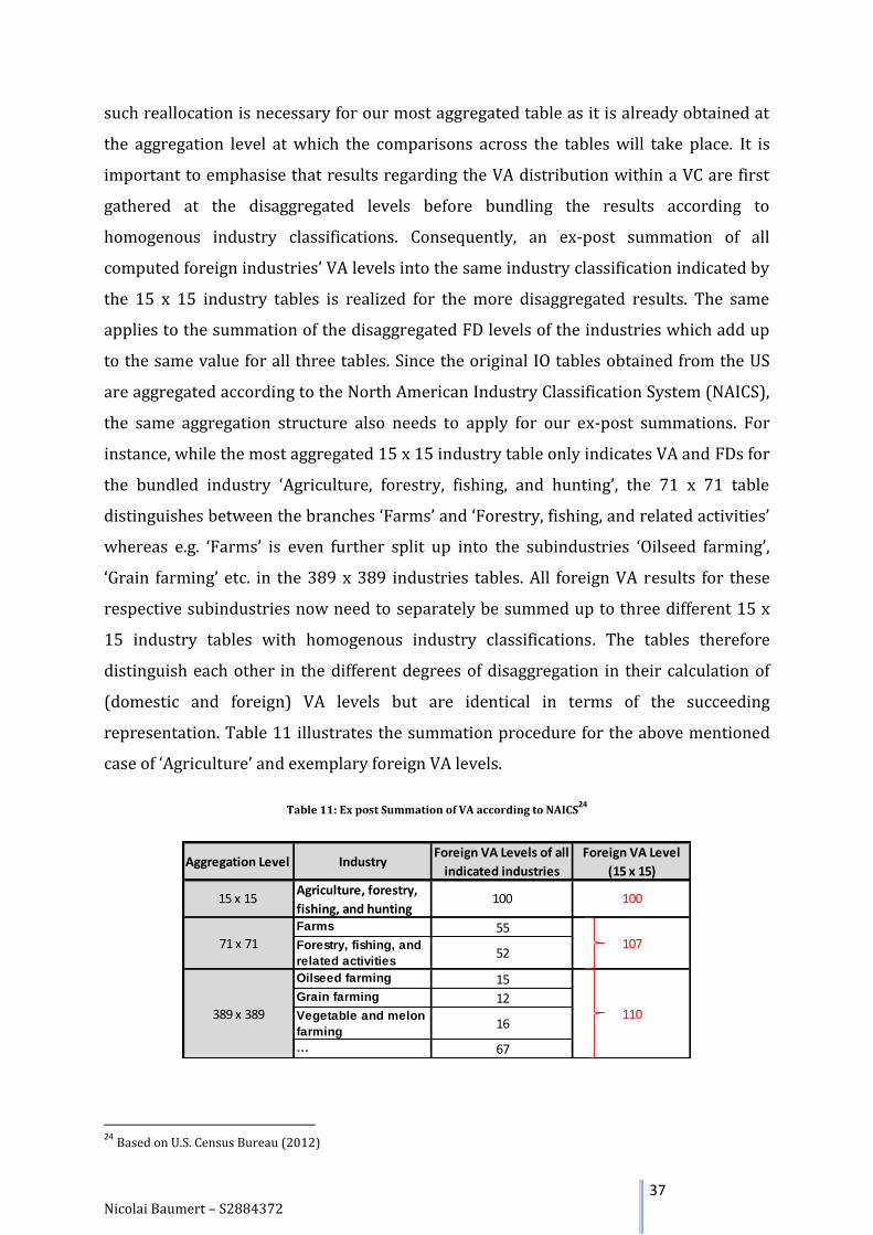
Nicolai Baumert – S2884372
37
such reallocation is necessary for our most aggregated table as it is already obtained at
the aggregation level at which the comparisons across the tables will take place. It is
important to emphasise that results regarding the VA distribution within a VC are first
gathered at the disaggregated levels before bundling the results according to
homogenous industry classifications. Consequently, an ex-post summation of all
computed foreign industries’ VA levels into the same industry classification indicated by
the 15 x 15 industry tables is realized for the more disaggregated results. The same
applies to the summation of the disaggregated FD levels of the industries which add up
to the same value for all three tables. Since the original IO tables obtained from the US
are aggregated according to the North American Industry Classification System (NAICS),
the same aggregation structure also needs to apply for our ex-post summations. For
instance, while the most aggregated 15 x 15 industry table only indicates VA and FDs for
the bundled industry ‘Agriculture, forestry, fishing, and hunting’, the 71 x 71 table
distinguishes between the branches ‘Farms’ and ‘Forestry, fishing, and related activities’
whereas e.g. ‘Farms’ is even further split up into the subindustries ‘Oilseed farming’,
‘Grain farming’ etc. in the 389 x 389 industries tables. All foreign VA results for these
respective subindustries now need to separately be summed up to three different 15 x
15 industry tables with homogenous industry classifications. The tables therefore
distinguish each other in the different degrees of disaggregation in their calculation of
(domestic and foreign) VA levels but are identical in terms of the succeeding
representation. Table 11 illustrates the summation procedure for the above mentioned
case of ‘Agriculture’ and exemplary foreign VA levels.
Table 11: Ex post Summation of VA according to NAICS24
24
Based on U.S. Census Bureau (2012)
Aggregation Level IndustryForeign VA Levels of all
indicated industries
Foreign VA Level
(15 x 15)
Farms 55Forestry, fishing, and
related activities52
Oilseed farming 15Grain farming 12Vegetable and melon
farming16
… 67
100
107
389 x 389 110
15 x 15 Agriculture, forestry,
fishing, and hunting100
71 x 71

Nicolai Baumert – S2884372
38
Obviously, the same industrial classification applies to the summation of FDs which is
not illustrated separately. Only when proceeding accordingly for all industries will it be
possible to compare the VA results derived from different extents of aggregation on an
equal, more aggregated industry level. From this reallocation of VA levels we
subsequently obtain the FVAS for each of the 15 industries in a specifiable scenario with
regards to the IS and the country number IS for each level of initial disaggregation
computed in line with equation (2). Let us recall that we aim to derive the extent to
which N&V’s (2014) biases distort the VA distribution. Since these biases are based on
the aggregation of VCs into bundled sets of these, the deviation from our disaggregated
table (containing the true VA distribution) is attributable to the distortion of the FVASs.
6. RESULTS
In order to visualise the differences in the results for FVASs across our IO tables based
on different extents of aggregation, we display tables in which the respective FVASs are
subtracted from each other. The first represented scenario in Table 12 shows a set-up
with 10 countries and the variations between the FVASs of the most aggregated 15-
industry IO table and the respective true shares derived from our 389 x 389 industry IO
table. Therefore, it indicates the magnitude of the distortion from the empirical
equivalent of Table 5 without any merged VCs25. The interpretation of the included
values within the table follows the ensuing principles. Since we display the results
arising when the simulated FVAS of the aggregated IO table is subtracted from the one in
the table containing the true VA distribution, negative values indicate that the FVAS is
misrepresented as too high (overstated) in our aggregated tables. In turn, this means
that the DVAS will be indicated as too (understated) low compared to its actual share.
Similarly, positive values express that DVASs for industries that relate to these values
are overestimated by our IO analysis whereas the FVASs would be underestimated.
25
Please note that the displayed values refer to percentage points (pp) as the absolute difference between the respective FVASs from the IO tables at different aggregation levels.

Nicolai Baumert – S2884372
39
Table 12: Deviation of true FVASs and FVASs from 15-industry Tables (10 Countries)(in pp)
The results for the 10-country case show mixed evidence of over- and understated
foreign industries’ VA contributions. More specifically, 6 of the 15 industries’ FVASs that
are compared across aggregation levels are overestimated in the case of an IS of 0.2. This
holds to a special degree for ‘Agriculture’, ‘Mining’ and ‘Finance’ (although, again, the
latter will most likely incorporate a lower IS in reality) for which the FVASs are
overstated by 3.1 up to 5.1 percentage points. Furthermore, the remaining industries
which exhibit an understatement of the FVAS due to bundling of VCs do not deviate
significantly across aggregation levels. An exception worth mentioning may be ‘Other
Services’ showing a FVAS which is underestimated by 1.9 percentage points when
derived from an aggregated table. Moreover, we find that rising internationalisation – in
the form of rising ISs – mostly raises the aggregated results’ exposure to the biases.
Despite these heterogeneous results across industries, the findings are in line with the
concepts developed by N&V (2014). For instance, agricultural production generally
forms a part of VCs which is very upstream and exhibits a high VA coefficient. Therefore,
when regarding ‘Agriculture’ as the industry delivering a final product, its VA that is
contributed at a downstream stage is mostly relatively limited. Consequently, the last
(domestic) industry would incorporate a particularly high VA coefficient which N&V
(2014) expect to be underestimated in such a scenario. The same principle applies for
‘Mining’ as well as for ‘Finance’ and subsequently results in an underestimated DVAS for
the respective country-of-completion. In contrast, most personal service industries show
positive values in Table 12 representing an overstated VA contribution of the domestic
country for an empirically relevant range of ISs. Since these industries contribute to
production processes relatively further downstream in most cases, a low VA coefficient
leads to the overestimation of the DVAS as also proclaimed by N&V (2014).
10 Countries
comparing
15x15 and
389x389
industries
Agri-
culture,
forestry,
fishing,
and
hunting
Mining Utilities Construc-
tion
Manu-
facturing
Whole-
sale
trade
Retail
trade
Transport
and ware-
housing
Infor-
mation
Finance,
insurance,
real estate,
rental, and
leasing
Profes-
sional &
business
services
Education,
health
care, and
social
assistance
Arts,
enter-
tainment
etc.
Other
services,
except
govern-
ment
Govern-
ment
IS 0.10 -2.80 -1.66 -0.05 0.24 0.18 0.19 0.38 0.52 -0.12 -1.63 -0.03 0.26 0.50 1.13 0.10
IS 0.20 -5.05 -3.09 -0.08 0.34 0.07 0.29 0.58 1.00 -0.24 -3.16 -0.13 0.39 0.73 1.89 0.14
IS 0.30 -6.86 -4.32 -0.10 0.36 -0.19 0.32 0.66 1.43 -0.35 -4.60 -0.28 0.43 0.78 2.40 0.15
IS 0.40 -8.35 -5.40 -0.11 0.34 -0.51 0.32 0.66 1.79 -0.45 -5.96 -0.44 0.42 0.72 2.74 0.13
IS 0.50 -9.57 -6.36 -0.13 0.30 -0.85 0.28 0.59 2.07 -0.53 -7.24 -0.63 0.37 0.59 2.93 0.10
Nicolai Baumert – S2884372
40
In order to verify if this explanation is consistent, we employ an indicator by Fally
(2012) computing the average number of VC stages between a good’s generation and the
consumption by the FD in our most disaggregated IO table as a measure of
upstreamness. Thereby we aim to confirm that e.g. most agricultural branches show a
high degree of upstreamness while personal services are mostly situated further
downstream within VCs. In line with Fally (2012), we use the equation
d = (I – B)-1e (8)
in which the elements bi j denote the ration between an industry i’s gross output and the
intermediate deliveries from industry i to j. Furthermore, d represents a SN x 1 vector
indicating the average VC stages until final consumption of the respective product. As
assumed, the mean VC length of subindustries differs largely across the aggregated
industries and amounts to 2.84 for ‘Agriculture’, yields 2.19 for ‘Manufacturing’ and
shows 1.05 for ‘Education’. This confirms our expectations and is in accordance with the
explanation of the heterogeneous directions of the FVASs distortion across industries.
Moreover, it emphasises another feature of our analysis compared to N&V’s (2014)
method since our simulations draw on empirically derived VC lengths whereas N&V
(2014) construct VCs with an average length of four which seems longer than in reality
according to the computation of Fally’s (2012) upstreamness indicator.
Considering the magnitude to which FVASs are also distorted in other empirically
relevant global set-ups with different country numbers shows only little difference to
the values indicated in the 10-country case26. This could be expected since Table 9 and
10 already established that the occurrence of production cycles only differs slightly in
multi-country scenarios which is due to the limited length and therefore bounded
potential fragmentation of VCs.
Expanding our analysis by considering the distortion of the 71-industry case as
displayed in Table 13 yields mostly similar results compared to the biases in the VA
distribution based on the 15-industry table. It is worth mentioning, however, that the
mean distortion of the FVASs in the less aggregated table (0.57 percentage points for IS
of 0.2) is significantly smaller when compared to the 15-industry case (1.14 percentage
26
The simulation results displaying the magnitude of the discussed biases in a scenario with 5 countries can be found in Appendix’ Table 15 which follows the same interpretive logic than Table 12.
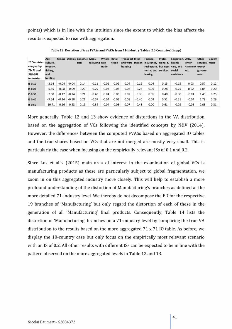
Nicolai Baumert – S2884372
41
points) which is in line with the intuition since the extent to which the bias affects the
results is expected to rise with aggregation.
Table 13: Deviation of true FVASs and FVASs from 71-industry Tables (10 Countries)(in pp)
More generally, Table 12 and 13 show evidence of distortions in the VA distribution
based on the aggregation of VCs following the identified concepts by N&V (2014).
However, the differences between the computed FVASs based on aggregated IO tables
and the true shares based on VCs that are not merged are mostly very small. This is
particularly the case when focusing on the empirically relevant ISs of 0.1 and 0.2.
Since Los et al.’s (2015) main area of interest in the examination of global VCs is
manufacturing products as these are particularly subject to global fragmentation, we
zoom in on this aggregated industry more closely. This will help to establish a more
profound understanding of the distortion of Manufacturing’s branches as defined at the
more detailed 71-industry level. We thereby do not decompose the FD for the respective
19 branches of ‘Manufacturing’ but only regard the distortion of each of these in the
generation of all ‘Manufacturing’ final products. Consequently, Table 14 lists the
distortion of ‘Manufacturing’ branches on a 71-industry level by comparing the true VA
distribution to the results based on the more aggregated 71 x 71 IO table. As before, we
display the 10-country case but only focus on the empirically most relevant scenario
with an IS of 0.2. All other results with different ISs can be expected to be in line with the
pattern observed on the more aggregated levels in Table 12 and 13.
10 Countries
comparing
71x71 and
389x389
industries
Agri-
culture,
forestry,
fishing,
and
hunting
Mining Utilities Construc-
tion
Manu-
facturing
Whole-
sale
trade
Retail
trade
Transport
and ware-
housing
Infor-
mation
Finance,
insurance,
real estate,
rental, and
leasing
Profes-
sional &
business
services
Education,
health
care, and
social
assistance
Arts,
enter-
tainment
etc.
Other
services,
except
govern-
ment
Govern-
ment
IS 0.10 -3.14 -0.04 -0.04 0.14 -0.11 -0.02 -0.02 0.04 -0.16 0.04 0.15 -0.15 0.03 0.57 0.12
IS 0.20 -5.65 -0.08 -0.09 0.20 -0.29 -0.03 -0.03 0.06 -0.27 0.05 0.28 -0.25 0.02 1.05 0.20
IS 0.30 -7.68 -0.12 -0.14 0.21 -0.48 -0.04 -0.03 0.07 -0.35 0.05 0.40 -0.30 -0.01 1.45 0.25
IS 0.40 -9.34 -0.14 -0.18 0.21 -0.67 -0.04 -0.03 0.08 -0.40 0.03 0.51 -0.31 -0.04 1.79 0.29
IS 0.50 -10.71 -0.16 -0.23 0.19 -0.84 -0.04 -0.03 0.07 -0.43 0.00 0.61 -0.29 -0.08 2.08 0.31

Nicolai Baumert – S2884372
42
10
countries
com-
paring 71
and 389
industries
Wood
pro-
ducts
Non-
metallic
mineral
pro-
ducts
Primary
metals
Fabri-
cated
metal
pro-
ducts
Machi-
nery
Com-
puter
and
elec-
tronics
Elec-
trical
equip-
ment
etc.
Motor
vehicles,
bodies
and
trailers
Other
trans-
port
equip-
ment
Furni-
ture
and
related
pro-
ducts
Miscel-
laneous
manu-
facturing
Food and
beverage
and
tobacco
products
Textile
mills
etc.
Apparel
and
leather
Paper
pro-
ducts
Printing
and
related
support
activi-
ties
Petro-
leum
and
coal
Che-
mical
pro-
ducts
Plastic
and
rubber
IS 0.20 -0.29 -2.19 -18.75 -1.53 -0.52 1.25 0.42 0.99 1.02 0.43 1.94 -0.66 1.21 0.57 -1.21 0.36 0.17 -7.19 2.00
Table 14: Deviation of true FVASs and their Values from 71 x 71 Tables for Manufactures branches (10 Countries) (in pp)
Table 14 generally exhibits rather small deviations between the true VA distribution and
the more aggregated classification but also shows two exceptions. With an
underestimation of the domestic VA by 18.8 and 7.2 percentage points, respectively, the
branches ‘Primary metals’ and ‘Chemical Products’ clearly diverge largely from their
actual VA contribution when regarding ‘Manufacturing’ as the industry-of-completion.
The reasoning is similar to the previous elaboration on the results for the 15-industry
aggregation level (e.g. for Agriculture). Again, the cause for the relatively large distortion
is found in the very strong upstreamness27 of most ‘Primary metals’ and ‘Chemical
Products’ subindustries which results in a high VA coefficient and the understatement of
the respective branch’s VA contribution in line with N&V (2014).
Despite the fact that results regarding the generated VA of these branches may
potentially be biased and require caution as they distort studies regarding the FVASs of
final manufacturing products as examined in Los et al. (2015), we must also note that
the contribution of these (especially of the most distorted branch ‘Primary metals’) as a
share of the overall final output of ‘Manufacturing’ is rather limited28.
Therefore, although we find selected industrial branches that show a larger distortion
based on their high upstreamness, their relative importance for indicators as introduced
in Los et al. (2015) seems rather limited. Since the same applied for the distortion of the
VA distribution found for the most aggregated 15-industry case, we can summarise the
results by stating that the biases identified by N&V (2014) can also be detected in an
empirical analysis. Their magnitude and direction vary largely depending on the
upstreamness of the respective sector’s subindustries but is mostly found to be of minor
relative importance. Referring back to the research question that formed the outline for
this paper, we do not find that the biases in the IO concepts significantly distort findings
of studies which examine the VA distribution in globally fragmented VCs.
27
The previously introduced upstreamness indicator by Fally (2012) yields average values of 3.76 for ‘Primary metals’ and 2.98 for ‘Chemical Products’ within the computed vector d. 28
The final output of ‘Primary metals’ forms 2.6 percent of final ‘Manufacturing’ output while the final output of ‘Chemical products’ amounts to 7.2 percent thereof.

Nicolai Baumert – S2884372
43
7. CONCLUDING REMARKS
This paper addressed the reliability of findings regarding the VA distribution in global
production fragmentation studies which employ IO analysis. N&V (2014) identified
biases that arise from the aggregation of VCs into sets of these. Following from
simulations based on VCs that are largely constructed by randomisations, they argue
that the VA contribution of the industry-of-completion will be understated if this
industry mostly appears at upstream production stages in VCs. In turn, the VA of
industries which generally contribute to VCs at a downstream stage will be
overestimated. We extend N&V’s (2014) analysis by employing empirical data on
different levels of aggregation to examine the biases’ magnitude for realistic production
processes. Thereby, we are guided by the following research question:
Do the biases identified by Nomaler & Verspagen (2014) significantly distort the empirical
findings of studies examining the value added distribution in globally fragmented
production processes if input-output analysis is employed?
Other than N&V (2014), we are able to base our simulations of IO measurements for VA
distribution on empirically observed VCs as well as their underlying characteristics and
succeed in quantifying the empirical extent to which these distributions are biased. We
conclude by presenting our main outcome, clarifying the limitations of our analysis and
suggesting future research in line with our study.
7.1. MAIN FINDINGS
The major contribution of this paper is the fact that it extends N&V’s (2014) analysis of
aggregation biases by an empirical component. Based on national IO data that we
transformed into hypothetical global set-ups, we constructed several scenarios with
regards to the number of countries and the degree to which these engage in
international trade. Moreover, we improved N&V’s (2014) analysis by relying on
realistic VCs. We find that the length of VCs is generally shorter than assumed by N&V
(2014) and that their constructed ‘snake’-shaped VCs do not match the empirical
pattern. Moreover and other than N&V (2014), the order and upstreamness of
industries’ appearances as well as their VA contribution within VCs is naturally derived
from actual production processes. These improvements allow for a more profound
analysis of the distortion’s empirical relevance.

Nicolai Baumert – S2884372
44
Despite these differences in the approaches our results are largely in line with the
analysis of N&V (2014) as we find that the empirical direction and extent of the
distortions of indicators like the domestic value added share by Los et al. (2015) depend
on the general upstreamness of the regarded industry. Thus, examining the VA
contribution for VCs whose industry-of-completion generally appears far upstream in
VCs (e.g. agriculture, mining or finance) will cause an overstatement of the FVAS. In
contrast, analysing VCs whose industry-of-completion mostly contributes to VCs at
production stages that are close to the consumption of the good (e.g. personal services
like education or entertainment) may result in an overstatement of the domestic
contribution share. A similar pattern also holds when regarding the distortion of
branches of the ‘Manufacturing’ industry more specifically which are generally most
exposed to global production fragmentation.
The distortions of the FVASs are most pronounced in scenarios of high international
trade but hardly differ with the number of countries. The latter is due to the fact that we
find the average number of VC stages before the final product’s consumption to be
rather limited which decreases the potential for its fragmentation. In terms of the
magnitude of the biases, our results differ from those obtained by N&V (2014). For
empirically relevant degrees of ISs, our comparisons between the true VA distribution
and the results for the analysis based on the most aggregated industry classification
yield an overstatement of the FVASs by 5 percentage points at most whereas N&V
(2014) expect the bias to be far more influential. The distortion of most industries’ VA
contributions ranges between plus and minus 1 percentage points which is only
surpassed by the industries which show the most distinct general pattern of up- (e.g.
Agriculture and Mining) or downstreamness (e.g. Other Services). Comparing across
different degrees of the bundling of VCs, we find that the mean distortions indeed
increase with aggregation (from the 71 to a 15-industry level) in line with the nature of
the biases but do not change their magnitude drastically.
7.2. LIMITATIONS AND FUTURE RESEARCH SUGGESTIONS
Although we employed empirical data for our analysis, it stills builds upon several
assumptions and limitations which restrict the scope of our paper but could potentially
be relaxed in more extensive studies. First, we purely based our evaluations on US-
American IO data. Consequently, the underlying VC structures are exclusively subject to
Nicolai Baumert – S2884372
45
the domestic production technology and do not reflect global diversity in international
production processes. This does not allow for differences in the extent to which the
distortions affect the VA distribution in production processes across countries of equal
size. For instance, differences in the industries general up- and downstreamness across
countries may increase or decrease the distortion’s extent in line with our explanations
of the biases’ principles. Second, the regarded global scenarios are limited to countries of
the same economy size as well as equal ISs. This assumption clearly does not hold in
reality where countries’ economic dimensions and their exposure to international trade
largely vary. Differences in the magnitude of the distortions could for instance arise
when comparing small and larger economies. More specifically, smaller countries may
be particularly exposed to the biases due to a mostly high degree of internationalisation.
Third, we focused on the extent of distortions based on one single year’s observations.
No dynamic component is incorporated in our analysis although it may be meaningful to
examine the empirical magnitude of the identified biases when comparing multiple
years and their industries’ respective FVASs. N&V (2014) assume changes in the FVASs
to be understated whereas our results rather suggest the opposite. We call for an
empirical verification of this conjecture. Lastly, this study assumes equal degrees of
tradability across industries which is far from reality where personal service industries
mostly exhibit significantly smaller import shares than other sectors (e.g.
manufacturing). Accounting for this would not only change the results for the VA
distribution of industries whose IS would be altered but the interdependences among
industries would likely also cause differences for the remaining sectors. For instance,
since service industries mostly appear further downstream in VCs, decreases in the
tradability of their goods may contribute to an overstatement of the domestic VA shares.
As far as future research and extensions of our approach are concerned, we encountered
a data issue when allocating specific intermediate inputs to our most disaggregated IO
table. Our rather simple method to solve the problem by assigning the related values to
the intermediate and FD matrix in proportion to the total intermediate deliveries could
be improved upon in later studies. Moreover, it may be meaningful to alter the applied
aggregation levels in line with industrial classifications of major databases (e.g. 35
industries in the WIOD) to enable the examination of the distortions’ magnitude at
aggregation levels that are more commonly used for economic studies based on IO
analysis. In line with the limitations, our assumptions of homogeneous country size as

Nicolai Baumert – S2884372
46
well as ISs across sectors also clearly do not hold in reality and could be relaxed (e.g. by
assuming no tradability of service industries) as part of future research. Furthermore, it
may be worthwhile to extend the scope of the distortions’ analysis to the influence on
other IO-based indicators focusing on VA and its global trade (e.g. Johnson & Noguera,
2012a). These may also be affected by the regarded biases although the extent of the
distortion is likely to be highest when investigating specific VCs as part of the GVC
approach as e.g. in Los et al. (2015). Lastly, examining the magnitude to which the
identified distortions affect the results about changes in the VA distribution between
two points in time might shed even more light on the distortion’s dynamic nature.
Nicolai Baumert – S2884372
VI
REFERENCES
Amador, J., & Cabral, S. (2009). Vertical specialization across the world: A relative
measure. The North American Journal of Economics and Finance, 20(3), 267-280.
Baldwin, R., & Lopez‐Gonzalez, J. (2015). Supply‐chain Trade: A Portrait of Global
Patterns and Several Testable Hypotheses. The World Economy, 38(11), 1682-1721.
Baldwin, R., & Venables, A. J. (2013). Spiders and snakes: offshoring and agglomeration
in the global economy. Journal of International Economics, 90(2), 245-254.
Buckley, P. J., & Ghauri, P. N. (2004). Globalisation, economic geography and the strategy
of multinational enterprises. Journal of International Business Studies, 35(2), 81-98.
Dedrick, J., Kraemer, K. L., & Linden, G. (2010). Who profits from innovation in global
value chains? A study of the iPod and notebook PCs. Industrial and Corporate Change,
19(1), 81-116.
Dietzenbacher, E., Los, B., Stehrer, R., Timmer, M., & De Vries, G. (2013). The construction
of world input–output tables in the WIOD project. Economic Systems Research, 25(1), 71-
98.
Dudenhöffer, F. (2005). Wie viel Deutschland steckt im Porsche?. ifo Schnelldienst,
58(24), 03-05.
Fally, T. (2012). Production staging: measurement and facts. Boulder, Colorado,
University of Colorado Boulder, May.
Feenstra, R. C., & Hanson, G. H. (1999). The impact of outsourcing and high-technology
capital on wages: estimates for the United States, 1979-1990. Quarterly Journal of
Economics, 907-940.

Nicolai Baumert – S2884372
VII
Gereffi, G. (1989). Development strategies and the global factory. The Annals of the
American Academy of Political and Social Science, 92-104.
Grunwald, J., & Flamm, K. (1985). The global factory: Foreign assembly in international
trade. The International Executive, 27(3), 19-20.
Guo, J., Lawson, A. M., & Planting, M. A. (2002). From Make-Use to Symmetric IO Tables:
An Assessment of Alternative Technology Assumptions (No. 0021). Bureau of Economic
Analysis.
Horowitz, K. J., & Planting, M. A. (2006). Concepts and methods of the input-output
accounts (No. 0066). Bureau of Economic Analysis.
Hummels, D., Ishii, J., & Yi, K. M. (2001). The nature and growth of vertical specialization
in world trade. Journal of international Economics, 54(1), 75-96.
Johnson, R. C., & Noguera, G. (2012a). Accounting for intermediates: Production sharing
and trade in value added. Journal of International Economics, 86(2), 224-236.
—— (2012b). Fragmentation and Trade in Value Added over Four Decades. NBER
Working Paper Series, 18186.
Koopman, R., Wang, Z., & Wei, S. J. (2014). Tracing Value-Added and Double Counting in
Gross Exports. American Economic Review, 104(2), 459-94.
López González, J. (2012). Vertical specialisation and new regionalism.
Department of Economics, University of Sussex, No. 0212.
Los, B., Timmer, M. P., & Vries, G. J. (2015). How global are global value chains? A new
approach to measure international fragmentation. Journal of Regional Science, 55(1), 66-
92.

Nicolai Baumert – S2884372
VIII
Los, B. (2016). The Growing Importance of Input-Output Analysis for our Understanding
of International Trade. In T. ten Raa (Ed.), Elgar Handbook of Input-Output Analysis.
Cheltenham: Edward Elgar, forthcoming.
Nomaler, Ö., & Verspagen, B. (2014). Analysing global value chains using input-output
economics: Proceed with care. UNU-MERIT Working Papers, 70.
OECD–WTO. (2012) Measuring Trade in Value-Added: An OECD-WTO Joint Initiative.
Retrieved on 15 February 2016 from http://www.oecd.org/sti/
industryandglobalisation/measuringtradeinvalue-addedanoecd-wtojointinitiative.htm.
Timmer, M. P., Los, B., Stehrer, R., & De Vries, G. J. (2013). Fragmentation, incomes and
jobs: an analysis of European competitiveness. Economic Policy, 28(76), 613-661.
Timmer, M. P., Erumban, A. A., Los, B., Stehrer, R., & de Vries, G. J. (2014). Slicing up
global value chains. The Journal of Economic Perspectives, 28(2), 99-118.
Timmer, M. P., Dietzenbacher, E., Los, B., Stehrer, R., & Vries, G. J. (2015). An illustrated
user guide to the world input–output database: the case of global automotive
production. Review of International Economics, 23(3), 575-605
U.S. Census Bureau (2012). North American Industry Classification System. Retrieved on
25 May 2016 from http://www.census.gov/eos/www/naics
Wang, Z., Wei, S. J., & Zhu, K. (2014). Gross trade accounting: A transparent method to
discover global value chain-related information behind official trade data: Part 2. Vox EU,
16.

Nicolai Baumert – S2884372
IX
APPENDIX
Table 15: Deviation of true FVASs and their Values from aggregated 15-industry Tables for 5 Country case (in pp)
5 Countries
comparing
15x15 and
389x389
industries
Agri-
culture,
forestry,
fishing,
and
hunting
Mining Utilities Construc-
tion
Manu-
facturing
Whole-
sale
trade
Retail
trade
Transport
and ware-
housing
Infor-
mation
Finance,
insurance,
real estate,
rental, and
leasing
Profes-
sional &
business
services
Education,
health
care, and
social
assistance
Arts,
enter-
tainment
etc.
Other
services,
except
govern-
ment
Govern-
ment
IS 0.10 -2.76 -1.65 -0.05 0.23 0.16 0.19 0.37 0.52 -0.12 -1.62 -0.04 0.25 0.48 1.10 0.10
IS 0.20 -4.92 -3.03 -0.08 0.31 0.01 0.27 0.54 0.99 -0.24 -3.14 -0.15 0.36 0.67 1.81 0.13
IS 0.30 -6.63 -4.21 -0.09 0.32 -0.27 0.29 0.60 1.40 -0.34 -4.55 -0.30 0.38 0.68 2.26 0.13
IS 0.40 -7.99 -5.24 -0.11 0.28 -0.60 0.27 0.56 1.73 -0.44 -5.87 -0.47 0.35 0.59 2.53 0.10
IS 0.50 -9.09 -6.14 -0.13 0.24 -0.94 0.22 0.47 1.97 -0.51 -7.11 -0.66 0.29 0.43 2.67 0.06