assessing the risk of violating stream water quality
TRANSCRIPT
1988
ASSESSING THE RISK OF VIOLATING STREAM WATER QUALITY STANDARDS
Wade E. Hathhorn Yeou-Koung Tung
Journal Article WWRC-88-12
In
Journal of Environmental Management
Volume 26
1988
Wade E. Hathhorn Department of Civil Engineering
Yeou-Koung Tung Wyoming Water Research Center and Department of Statistics
University of Wyoming Laramie, Wyoming

- Journal of Environmental Management (1 988) 26, 32 1-338
Assessing the Risk of Violating Stream Water Quality Standards
Wade E. Hathhornt and Yeou-Koung Tungt
?Department of Civil Engineering, $ Wyoming Water Research Center and Department of Statistics, University of Wyoming, Laramie, Wyoming 82071, U.S.A.
Received 12 May 1986
For many years, managing agencies have enacted and enforced water quality standards based on a deterministic evaluation of the stream environments under their control. Given the random nature of the processes occurring within a stream system, the deterministic approach to water quality regulation is subject to obvious shortcomings. In an attempt to improve water quality regulation, a method is presented for quantifying the joint risk associated with dissolved oxygen deficits exceeding a specified standard and the length of such violations within a stream environment. Techniques are employed utilizing the Streeter-Phelps equation in conjunction with Monte Carlo simulation. In addition, flexibility is provided in the formulation by allowing several probability distributions to be assigned to each parameter in the model. A sensitivity analysis is also performed on the joint risk for the various probability distributions and statistical properties assumed for each parameter. Implied in the methods and results presented is the development of improved water quality standards incorporating the inherent stochastic nature of stream environments.
Keywords: dissolved oxygen, biochemical oxygen demand, S treeter-Phelps equation, Monte Carlo simulation, risk assessment, probability distributions, uncertainty, water quality standards.
1. Introduction
Although technology has greatly improved our ability to treat industrial and municipal wastes, it is still a common practice to discharge allowable quantities of pollution from these effluents into various watercourses. This practice is based on the principle that the receiving waters possess a natural ability to assimilate a specific quantity of pollutant. Given these conditions, the allowable waste concentrations and natural biota coexist within the dynamic environment of the stream system. Consequently, water quality officials have been given the arduous task of determining the socioeconomic tradeoffs between allowable waste load allocations and maintaining desired levels of aquatic life within the stream environment. In answer to these problems, water quality agencies have enacted regulations allowing the continuation of waste discharge to streams subject to a variety of water quality standards.
32 1
0301-4797/88/040321+ 18 $03.00/0 0 1988 Academic Press Limited

,
322 Stream water quality stamlards
In contrast to the fact that each stream is highly variable by nature, the basis for the development of water quality standards continues to be a deterministic evaluation of the stream environment. As a result, many of the present water quality standards neglect the inherent stochastic nature of the system (i.e. rivers and streams) which they are supposed to protect. Several authors, noting the shortcomings associated with present water quality standards, have criticized the ability of deterministic standards to provide adequate protection of the stream environment (Loucks and Lynn, 1966; Adams and Gemmel, 1975; Burn and McBean, 1985). Knowing the reality of the inherent random nature of these systems, deterministic standards should be amended to account for the stochastic processes present in the stream environment. In addition, most of the current standards do not differentiate between the various levels of exceedance or the lengths of violation in the stream system. Given the deterministic structure of present water quality regulations, it is implied that all water quality violations are considered equal, regardless of the effects on the stream environment. Presently, no emphasis is placed on the relative severity of the individual violations. For example, a small exceedance, resulting in minor damage, is treated in the same manner as a large exceedance, possibly resulting in significant damage. Both conditions are simply defined as “violations”, thus neglecting the relative effects created by the specific violation conditions.
In an attempt to incorporate the random nature of the stream environment and the level of severity for various violation conditions into the water quality decision-making process, it is the objective of this paper to present a methodology for evaluating the joint risk associated with a maximum dissolved oxygen deficit (beyond a specified standard) and the length of such violation within any given stream system. This study utilizes the simplified Streeter-Phelps equation and Monte Carlo simulation techniques to evaluate the risk, based on several assumptions for the probability distributions assigned to each parameter in the model formulation. In addition, a sensitivity analysis is performed to evaluate the effects of changes in the statistical characteristics of the model parameters on the risk. By evaluating the risks associated with water quality violatiohs, it is believed a more realistic decision can be made between the economic and environmental questions facing water quality management agencies in the future.
2. Water quality model
Within an aquatic environment, dissolved oxygen is present in conjunction with a certain quantity of waste. A common measure of the amount of waste present and relative aquatic health in a stream system is the biochemical oxygen demand (BOD) and concentration of dissolved oxygen (DO), respectively. Through the processes of biode- gradation and re-aeration, the stream exhibits a natural ability to assimilate a given quantity of BOD. The biological processes result in DO deficits which are replenished by the natural re-aeration of the stream. Several mathematical models have been developed to describe the physical, biological processes occurring within the stream environment. The most common expression is known as the Streeter-Phelps equations (Streeter and Phelps, 1925). In differential form, the equation is given as:
dD/dt = K , L - K2D. (1)
The solution to equation (l), replacing t by X / U , is:

W. E. Hathhorn and Yeou-Koung Tung 323
where KI is the deoxygenation coefficient, K, is the re-aeration coefficient, X is the distance downstream from the source of BOD, U is the average stream velocity, D(X) is the DO deficit concentration at a downstream distance X , Do is the initial DO deficit (at distance X=O), and Lo is the initial in-stream BOD concentration.
The concentration of DO at any downstream location is given as:
C(X) = c, - D ( X ) (3)
in which C, is the saturated DO concentration. The downstream location, Xc, where the maximum DO deficit occurs can be found by:
The point Xc will herein be referred to as the “critical location”. The associated maximum DO deficit is determined by:
Additionally, several assumptions should be noted in the development of the Streeter-Phelps equation: (a) steady, uniform flow; (b) DO deficits predicted by equation (2) are one-dimensional (functions only of the position downstream from a discharge point); and (c) rates of biodegradation and re-aeration, expressed by K, and K2, are described by first-order kinetics. A typical DO profile for a single reach is shown in Figure 1.
Figure 1. Typical dissolved oxygen sag curve.
Equation (2) describes the response of DO in a single reach of stream as a result of the addition of a “point-source” loading of waste at the upstream end of the reach. This equation can be used to determine the DO concentration in several successive reaches by applying the deficit at the downstream end of one reach as the initial deficit of the succeeding reach. Thus, equation (2) can be applied iteratively to determine the DO profile of an entire stream system (Liebman and Lynn, 1966).

Stream water quality standards 324
Since its conception, the Streeter-Phelps equation has been modified to account for discrepancies between analytical estimations, given by equation (2), and actual data collected in the field. These discrepancies have arisen as a result of the exclusion of a number of oxygen sources and sinks in the original equation. For example, the processes of sedimentation, benthic demand, photosynthesis, and algal respiration have been included to improve model predictability (Dobbins, 1964; Hornberger, 1980; Krenkel and Novotny, 1980). Modifications can be made by simply adding terms to equation (2) to account for these factors. However, in order to simplify the algebraic manipulations, the original Skeeter-Phelps equation is utilized in this study. It is simply the authors’ intention at this point to note the improvements made to the original equation by various other researchers, though by no means do the citations presented represent, in entirety, the wealth of information on this subject.
3. Uncertainty in the water quality model
The uncertainty associated with equation (2), for predicting DO level in stream systems, can be divided into three categories: inherent, parameter, and model uncertainties. Inherent uncertainties are the result of the natural randomness exhibited by the physical, biological processes described by equation (2). This inherent uncertainty is the product of temporal and spatial variations, for example, in streamflow, effluent waste concentra- tion, temperature, and in-stream biological composition (Churchill et al., 1962; Bansal, 1973; Wright and McDonnell, 1979). In addition, the absence of unlimited data describing the characteristics of the stream system results in insufficient information to estimate the parameters of the model with absolute certainty. The combined effects of inherent randomness and imperfect data collection result in parameter uncertainty in the model formulation.
As previously mentioned, several researchers have modified the original Streeter- Phelps equation to account for discrepancies between DO deficits predicted by the model and collected field data. Such discrepancies were the result of the original model’s exclusion of a number of oxygen sources and sinks. The inability of the model to predict accurately the DO deficits is known as model uncertainty. To account for this inadequacy, additional terms may be added to the model formulation to include the effects of the various oxygen sources and sinks. Alteratively, adjustment of the model may be accomplished by multiplying the original equation by a “model correction factor”. This correction factor would simply be determined from an analysis of the differences between the predicted and field data collected. The model correction factor can also be treated as a random variable in the model formulation. Although this approach is not used in this study, it is again simply the authors’ intention to point out deficiencies in the original model formulation [refer to equation (2)].
Given the fact that inherent, model, and parameter uncertainties exist, the stochastic nature of the stream system must be included in the model formulation if accurate DO predictability is to be attained. The general approach for describing these uncertainties has been to assign appropriate statistical properties, probability distributions, and correlations to each of the parameters in equation (2).
3.1. SELECTION OF STATISTICAL PROPERTIES FOR THE MODEL PARAMETERS
The selection of statistical properties include the appropriate determination of the mean, standard deviation, and possibly other higher moments for each of the model para-

W. E. Hathhorn and Yeou-Koung Tung 325
meters. In order to quantify the statistical properties accurately, existing physical, chemical, and biological data are analyzed according to standard statistical procedures. Data used in the analysis should be obtained from the specific site under investigation in order to preserve the uniqueness associated with various stream environments. Once the analysis has been performed, the resulting statistical properties become eligible for model applications.
3.2. SELECTION OF PROBABILITY DISTRIBUTIONS FOR THE MODEL PARAMETERS
Though several probability distributions are possible, the most common assumption is that each of the parameters in equation (2) follow a normal distribution (Kothandara- mann and Ewing, 1969; Burges and Lettenmaier, 1975; Esen and Rathbun, 1976). However, some investigators have utilized a variety of distributions to describe the random behavior of the parameters in equation (2) (Kothandaramann, 1970; Brutsaert, 1975). Clearly, a universal agreement as to the type of distribution to use for each parameter does not exist. Given the uniqueness of each site under investigation, there is no reason to expect all the parameters to follow a given distribution for every location. Thus, it would seem reasonable to develop a procedure that will allow the model to be flexible with regard to the selection of the probability distribution for each parameter. Following this approach, each parameter in the model of this study can by assigned one of five probability distributions: normal, log-normal, beta, gamma, and Weibull. By analyzing the recorded data describing the random nature of the stream environment for each site, an appropriate probability distribution can be selected for each parameter in the model.
3.3. CORRELATION BETWEEN MODEL. PARAMETERS
With exception to K2 and U , the model parameters in equation (2) are considered to be independent. There has been extensive research in the development of mathematical functions directly relating the re-aeration rate, K,, to the physical characteristics of the stream such as average velocity, U (Bansal, 1973). These research results demonstrate clearly that a positive correlation exists between the model parameters K2 and U. Hence, procedures are provided in the model formulation of this study which allow for the inclusion of such a correlation.
Additionally, some investigators have proposed a positive correlation between K , and K2 (Esen and Rathbun, 1976; Padgett, 1978). Though statistical analysis of a given data set may reveal a correlation between these parameters, it is the opinion of the authors of this study that the significance of this determination has no meaningful physical representation in the model formulation. The authors’ reasonings are based on the fact that K2 is solely a function of the physical characteristics of the stream, while Kl is characterized by the biological composition of the waste discharge and stream environment. It is assumed that these processes act independently within the stream system. Consequently, the authors feel that the correlation between K, and K2 is spurious and, as such, it is not considered in this study.
4. Measurement of water quality conditions
Presently, water quality standards are developed on the basis of maximum contaminant levels or minimum required concentrations, both of which are never to be violated. The

326 Stream water quality standards ,
concept of a deterministic basis is plausible and feasible, if the system has very little or no uncertainty involved. However, as previously mentioned, it seems unreasonable to continue the enforcement of water quality requirements that neglect the probability of violating these standards when the system involves many elements subject to significant uncertainty. Hence, in order to improve the basis for regulatory standards in the stochastic environment of the stream system, a measure of the probability associated with the violation of water quality regulations should be developed.
As it has been in the past, the most commonly used measure to indicate water quality conditions in a stream system is the extent to which BOD and/or DO concentrations exceed current water quality standards. The severity of these violations are related to the tolerance level of the stream’s biota to a given pollution concentration and length of stream (or time) the system is subjected to such Conditions. For example, the stream system may not be able to tolerate relatively large DO deficits for short lengths of violation or, conversely, small DO deficits for much longer violation distances. In actuality, a tradeoff exists between the allowable level of DO deficit and length of stream subject to these violation conditions. Thus, in order to provide a more complete analysis of the stream environment under violation conditions, both the DO deficit and the length of violation should be considered.
The measure adopted in this study to indicate the water quality condition of a stochastic stream system is the joint probability of simultaneously violating a specified DO concentration and tolerable length of violation. Both maximum and average DO violation conditions, in conjunction with actual violation distance, are considered as follows :
or
Risk = Pr(b’ 2 D1ol and XD 2 Xt0J
in which Pr( ) is the probability, 06, and B‘ are the maximum and average DO deficits exceeding water quality standards, respectively, XD is the actual length of violation, and DI,l and Xto, are the specified tolerances for DO deficit beyond the standard, and the length of violation in the stream system, respectively (refer to Figure 2).
From this information, water quality management agencies could introduce regula- tory measures that limit the maximum probability of violating the minimum dissolved oxygen standards. For example, an amended DO standard might read as follows: “the maximum probability of violating a minimum DO concentration by 1 mg/l or less for a distance of 2 miles shall not exceed 0.05”. Once the allowable risk level associated with various violation conditions is quantified, water quality officials can proceed with the determination of allowable waste load allocations for the various users of the stream environment.
5. Quantification of the risk of violation
5.1. DETERMINING THE DO DEFICIT AND LENGTH OF VIOLATION
In reference to Figure 2, the length of violation is defined as the distance within the stream system where the DO profile is below a specified minimum concentration. A

W. E. Hathhorn and Ymu-Koung Tung 327
C 0 .- t
? I-
@ C
0
I I I
xc Xe Downstream distance
Figure 2. Diagram of violation conditions.
o i ;iY
standard minimum DO concentration of 4.0 mg/l was used throughout this study. Because of the non-linearity presented in equation (2), an analytical solution to determine the length of violation is infeasible. To circumvent this problem, the Newton- Raphson numerical approximation technique was employed to solve the beginning and ending points of violation. By taking the difference between these two end points, the length of violation was determined.
The maximum DO deficit was calculated using equation (5). The corresponding maximum level exceeding a specified concentration was defined as the maximum DO deficit beyond such a standard. In addition, the average DO deficit (within the length of violation) was calculated by integrating equation (2) over the length of violation. Then, dividing this expression by the same length to obtain:
where X,, and Xe are the beginning and end points of violation, respectively, XD is the length of violation (XD = Xc - X,,).
5.2. MONTE CARLO SIMULATION
Monte Carlo simulation can be simply described as a sampling method used to approximate, through simulation, the solution of non-linear formulation which would otherwise be extremely tedious to solve by direct analytical methods. The foundation for such an application lies in the large number of trials or iterations that are performed on the proposed model. By performing these iterations, a sufficiently large sample size can be generated, from which a relatively accurate solution to the model can be predicted.
Monte Carlo simulation techniques have found many applications in the modeling of

328 Stream water quality standards ,
stochastic processes. The essence of the technique is to develop a model that satisfactor- ily represents the random process to be analyzed. Then, through the use of a digital computer and random number generator, a large number of iterations are performed on the model formulation. During these iterations, input data are generated randomly according to selected probability distributions for each parameter in the model. Once the iterations are complete, the generated isolation set can be analyzed entirely to determine its stochastic properties or the individual values may be used in further analysis (Brutsaert, 1975). The application of Monte Carlo simulation in quantifying the violation risk will be shown in succeeding sections.
5.3. QUANTIFYING THE RISK ASSOCIATED WITH VARIOUS VIOLATION CONDITIONS
As previously noted, the joint risk is defined as the probability of occurrence for a given pair of violation conditions (i.e. a maximum or average exceeding DO deficit and length of violiation). Again, direct analytical methods were infeasible as solution techniques to quantify these risks, so Monte Carlo simulation techniques were applied.
Various pairs of violation conditions were generated using equations (2), (4), (5) and (7). In order to describe the random characteristics of the input data, each parameter in the water quality model was assigned one of the five probability distributions utilized in this study (normal, log-normal, gamma, beta, and Weibull), along with their associated statistical properties. Through the use of Monte Carlo simulation and Newton- Raphson’s numerical technique, N pairs of violation conditions were generated for various DO deficits and lengths of violation. The risk was then calculated by simply computing the ratio of the number of simulation pairs that jointly exceeded a specified deficit and length of violation, n, to the total sample size, N , generated:
n N + 1 * risk=-
In order to choose an appropriate sample size, it was found that the joint probability of violating a specified pair of maximum deficit and length of violation differed only slightly for various sample sizes, N , between 500 and 2000. Thus, an intermediate number of N=999 was adopted as the satisfactory sample size in this study.
When applying Monte Carlo simulation to equations (2) and (3), it is possible to generate negative DO concentrations. Though the number of occurrences of such unrealistic values is low, methods should be included in the simulation procedures which constrain the DO concentrations to be greater than or equal to zero (Hornberger, 1980). In the methods utilized in this study, negative DO concentrations generated by simulation are simply ignored and replaced by another iteration until N (= 999) realistic conditions are established.
6. Example of application
To illustrate the approach, an example has been formulated using hypothetical data for each parameter in equation (2). The selection of the mean of the water quality model parameters was based on a general stream classification described as “low velocity” (Fair et al., 1968; Chadderton et al., 1982). In addition, the standard deviations for each of the model parameters were selected in accordance with the data presented by Chadderton et al. (1982). To complete the data set, a correlation coefficient, between K2

W. E. Hathhorn and Yeou-Koung Tung 329
and U, of 0.8 was adopted on the basis of the experimental data tabulated in the article by Isaacs et al. (1969). It should be noted that, when the correlation between K, and U is specified, a bivariate normal or log-normal distribution is used. A summary of the model input data for the parameters of this study is given in Table 1.
The joint probability of violation was evaluated for a combination of 15 maximum DO deficits, beyond the standard of 4.0 mg/l (ranging from 0.0 to 1.5 mgjl) and 15 lengths of violation (ranging from 0.0 to 30.0 miles). The resulting 225 pairs of violation conditions were used to construct a contour map of the joint risk associated with the given combinations of maximum DO deficits and length of violation (see Figure 3 as an example). In order to illustrate the sensitivity of the risk to varying statistical characteris- tics, the procedure was iterated by assigning a variety of probability distributions to each of the parameters in the model. Finally, the entire process was repeated to develop risk contour maps based on various combinations of average exceeding deficits and lengths of violation.
TABLE 1 . Summary of data for model parameters
Standard Parameter Units Mean deviation Remarks
7. Discussion of results
Figures 3-9 illustrate the contours of risk associated with the various assumptions for the probability distributions assigned to each parameter in equation (2) and the correlation between K2 and U. Each Figure is documented with a heading providing information about the type of distribution, mean, standard deviation, and correlation coefficient @) assumed for the parameters in the risk assessment. Several combinations were explored for the various types of distribution utilized in this study. However, for the purpose of illustrating the general results, only a sample of the contour maps are presented in this paper. In order to analyze the results of this study, the discussion will focus on the sensitivity of the risk to variations, with respect to the following factors: (a) the probability distribution assigned to the model parameters; (b) the correlation between K2 and U; and (c) the statistical properties assigned to each parameter. In the following discussion, Figure 3 will be used as a basis for the comparison of other figures given the number of previous studies which have utilized the assumptions of normal distribution and independency for all the model parameters. Though the sensitivity of DO response to changes in water quality parameters has been investigated by many researchers (Burges and Lettenmaier, 1975; Esen and Rathbun, 1976; Hornberger, 1980; Chadderton et al., 1982), this study provides an attempt to evaluate the effects of the uncertainty of model parameters on the risk of violating water quality standards.
7.1. SENSITIVITY OF THE RISK TO VARIATIONS IN PROBABILITY DISTRIBUTIONS
Initially, it is obvious from visual inspection of the Figures presented that the type of
330 Stream water quality standards
K; : normal (0.35,O.IO) Lo : normal (18-0, 1-00) K, : normal (0*70,0.20) Do : normal ( 1-00, Ox)) U : normal (10.0,3001 p (K2,U) : 0.00
i 1.50 I I I I I 0 E 1 9
1.25 0 +
'D
1.00 aJ n C
0 * 0.75 e L
C aJ
5 0.50
I 1
1- 0.0 6 --\
5 10 15 20 1 25 1 30
Violation distance, miles
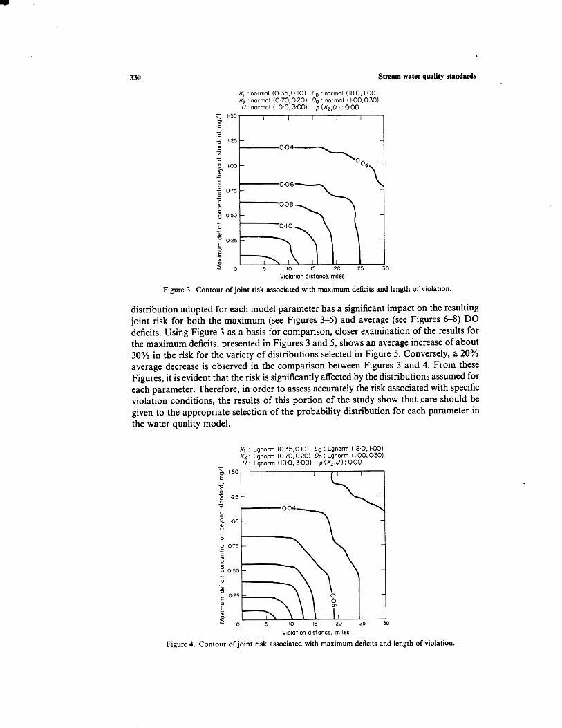
Figure 3. Contour of joint risk associated with maximum deficits and length of violation.
distribution adopted for each model parameter has a significant impact on the resulting joint risk for both the maximum (see Figures 3-5) and average (see Figures 6-8) DO deficits. Using Figure 3 as a basis for comparison, closer examination of the results for the maximum deficits, presented in Figures 3 and 5, shows an average increase of about 30% in the risk for the variety of distributions selected in Figure 5 . Conversely, a 20% average decrease is observed in the comparison between Figures 3 and 4. From these Figures, it is evident that the risk is significantly affected by the distributions assumed for each parameter. Therefore, in order to assess accurately the risk associated with specific violation conditions, the results of this portion of the study show that .care should be given to the appropriate selection of the probability distribution for each parameter in the water quality model.
K~ : Lgnorm (0.35,O.IO) Lo : Lgnarm (18.0,1~001 KZ : Lgnorm (0.70,0.20) Do : Lgnorm (1-00,0.30) U : Lgnorm (10.0,300) p ( K2,U) : 0.00
C .- + 2 0.75 t
W
C
2 0.50 c - * W 'D
0.25 5 E ._ X
f o I
10 15 20 25 5 1 30
10 15 20 25 5 Violation distance, miles
Figure 4. Contour of joint risk associated with maximum deficits and length of violation.

W. E. Hathhorn and Yeou-Koung Tung
KI : Normal (0.35,O.IO) Lo : Weibul (18.0, 1.00) K, : Lgnorm (0.70,0-20) Do : Beta (1.00,0.30) U : Gamma (10.0,300) p (Kz,U):O.OO
331
10 15 20 25 30 Violation distance, miles
Figure 5. Contour of joint risk associated with maximum deficits and length of violation.
A comparison of the risk contour maps for the average deficits (Figures 6-8) with those of the maximum deficits (Figures 3-5) shows an overall reduction in the risk associated with the average violation conditions. Intuitively, this result would be expected as the average DO deficit beyond the specified standard over the length of violation is lower than that of the maximum deficit. In addition, a comparison of the results from the average deficit conditions reveals the same general trends as those presented for the maximum deficits, thus reconfirming the sensitivity of the risk of violating water quality standards to the type of distribution assumed for each parameter in the water quality model.
Ki : Normal (0-35,O.IO) Lo : Normal (18.0, 1.00) K2 : Normal (0.70,0-20) DO : Normal ( 1.00, 0.30) U:Narmal (10.0, 3.00) p (K2,U) :0.00
1.25
U 5 1-00 a D C 0 + 0.75 2 c C V
0.50
0 5 10 15 20 25 30 Violation distance, miles
Figure 6. Contour of joint risk associated with average deficits and length of violation.
332 . Stream water quality standards
K, : Lqnorm (0.35,O-IO) Lo : Lgnorm ( 18.0, 1.00) K2 : Lqnorm (0.70,0-20) Do : Lgnorm (1.00,0~30) U : Lqnorm (100,300) p ( K2,U 1 : 0-00
c 0 + 0.75 e
9 0.50
c C 0
+ - u Y-
% 0.25
I 5 10 15 20 25 30 Violation dlstance, miles
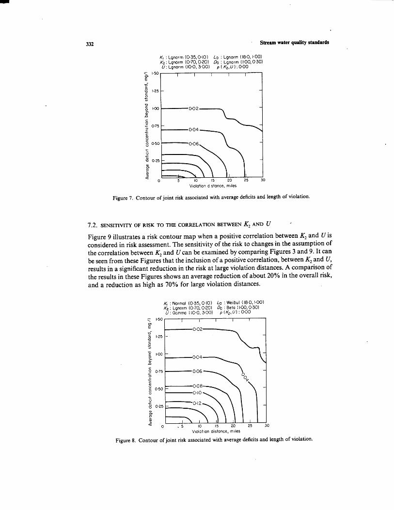
Figure 7. Contour of joint risk associated with average deficits and length of violation.
7.2. SENSITIVITY OF RISK TO THE CORRELATION BETWEEN K2 AND U Figure 9 illustrates a risk contour map when a positive correlation between K2 and U is considered in risk assessment. The sensitivity of the risk to changes in the assumption of the correlation between K2 and U can be examined by comparing Figures 3 and 9. It can be seen from these Figures that the inclusion of a positive correlation, between K2 and U, results in a significant reduction in the risk at large violation distances. A comparison of the results in these Figures shows an average reduction of about 20% in the overall risk, and a reduction as high as 70% for large violation distances.
/
Ki : Normal (0.35,O.IO) K2 : Lgnorm (0.70,O.ZO) U : Gamma ( 10.0,300)
Lo : Weibul (18-0, 1-00) Do : Beta ( 1.00,0.30)
p (Kz, U 1 : 000
c 0 0-75 & z f c 0)
2 0-50 V + - 0 'c 8 0.25
-
-
-
I 10 15 20 25 30 . 5 Violation distance, miles
Figure 8. Contour of joint risk associated with average deficits and length of violation.
W. E. Hathhorn and Yeou-Koung Tung 333
KI : Normal (0-35,O.IO) KZ : Normal (0-70,0.20) U : Normal (10.0, 300)
Lo : Normal (18.0,I.OO) Do : Normal (1.00,0.30)
p (K2,U) :0.80 -
e 1.25
0 c
C 0 $ 0-75 c
0)
c 2 0.50 + - U 'c
0.25 f
2 0
E X
c ? 0 ru
8 I, N
5 10 15 2 0 25 30 Violation distance, miles
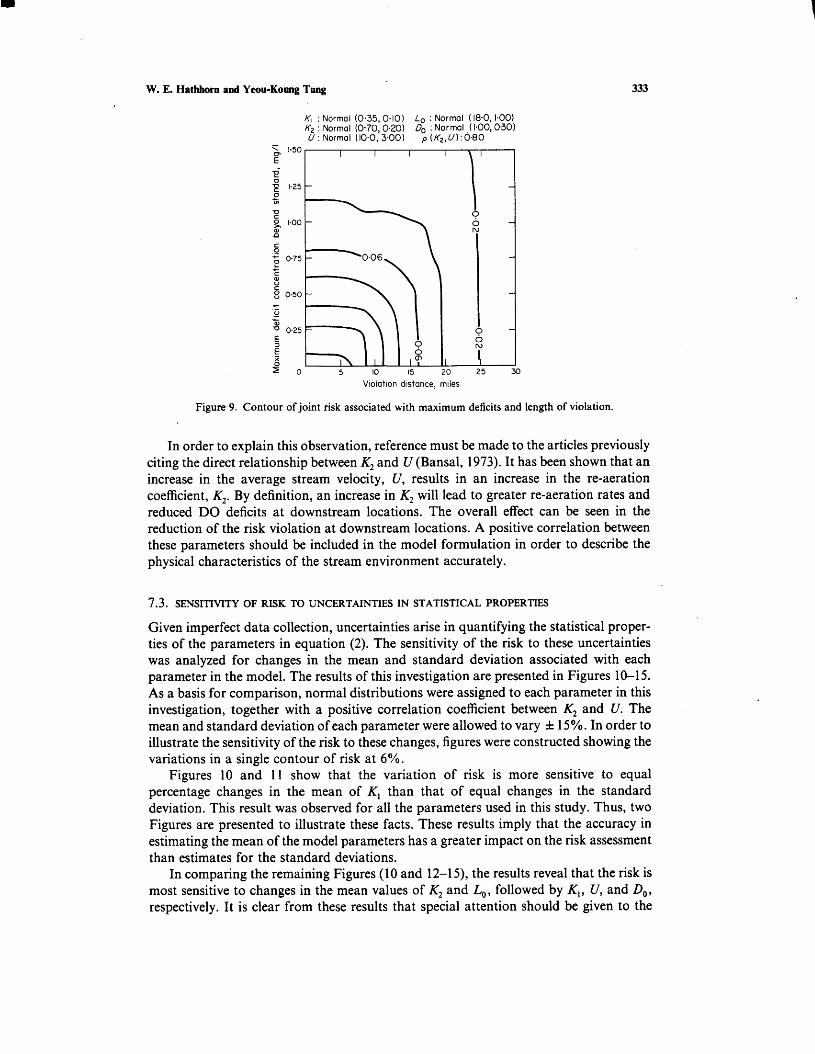
Figure 9. Contour of joint risk associated with maximum deficits and length of violation.
In order to explain this observation, reference must be made to the articles previously citing the direct relationship between K2 and U (Bansal, 1973). It has been shown that an increase in the average stream velocity, U, results in an increase in the re-aeration coefficient, K2. By definition, an increase in K2 will lead to greater re-aeration rates and reduced DO deficits at downstream locations. The overall effect can be seen in the reduction of the risk violation at downstream locations. A positive correlation between these parameters should be included in the model formulation in order to describe the physical characteristics of the stream environment accurately.
7.3. SENSITIVITY OF RISK TO UNCERTAINTIES IN STATISTICAL PROPERTIES
Given imperfect data collection, uncertainties arise in quantifying the statistical proper- ties of the parameters in equation (2). The sensitivity of the risk to these uncertainties was analyzed for changes in the mean and standard deviation associated with each parameter in the model. The results of this investigation are presented in Figures 1&15. As a basis for comparison, normal distributions were assigned to each parameter in this investigation, together with a positive correlation coefficient between K2 and U. The mean and standard deviation of each parameter were allowed to vary f 15%. In order to illustrate the sensitivity of the risk to these changes, figures were constructed showing the variations in a single contour of risk at 6%.
Figures 10 and 11 show that the variation of risk is more sensitive to equal percentage changes in the mean of K, than that of equal changes in the standard deviation. This result was observed for all the parameters used in this study. Thus, two Figures are presented to illustrate these facts. These results imply that the accuracy in estimating the mean of the model parameters has a greater impact on the risk assessment than estimates for the standard deviations.
In comparing the remaining Figures (10 and 12-1 5) , the results reveal that the risk is most sensitive to changes in the mean values of K2 and Lo, followed by K , , U, and Do, respectively. It is clear from these results that special attention should be given to the

334 Stream water quality standards
K, : Normol ( ,040) Lo : Normal ( I8-0,l.OO) Kz : Normal (0.70, Ox)) 0, : Normal ( 1~00,0~30) U : Normal (10-0, 300) p ( Kz.U 1 : 0-80 -
d -
-
-
- c 0*85K,
0.25 - .- c
E -
.-
5 I0 15 I 20 I 25 I 30 2 0
Violation distance, miles
Figure 10. Sensitivity of 6% risk with respect to the mean of K,.
Violation distance, miles
Figure 1 I . Sensitivity of 6% risk with respect to the standard deviation of K,.
determination of the mean values for K,, K,, and Lo, if accurate DO predictability is to be attained. It is evident from this portion of the study that proper selection of the statistical properties is crucial in order to quantify accurately the risk associated with the various violation conditions.

W. E. Hathhorn and Yeou-Koung Tung 335
I 1 I I
1.25 -
coo -
F
a
c .- c
'O 0.25-
.- I I I I
5 I0 I5 20 25 Vidation distance, miles
Figure 12. Sensitivity of 6% risk with respect to the mean of K2.
4 : Normal (0.3!5,0-10) Lo : Normal (18.0, 1.00) K2 : Normal (0*70,020) 4 : Normal (190,0*30) U : Normal ( , p ( K2,U):O-80
n
023 - E .- i
I I 1 I 1 5 10 I5 20 25
Violation distance, miles
Figure 13. Sensitivity of 6% risk with respect to the mean of U.
8. Summary and implications
This paper has presented a methodology for assessing the joint risk associated with maximum and average DO deficits exceeding specified standards and the length of such violations in stream systems receiving waste effluents. Moreover, this method allows this risk to be calculated on the basis of several assumptions about the type of probability distributions assigned to each parameter in the Streeter-Phelps equation. The flexibility provided by this type of model formulation permits a unique analysis of each site under investigation.

336
E" f 2- 1-25 0 c
1 1.00 2
Stream water quality staodards
I I I I I
- -
- -
c
8 c 0.50 - +. .c
.-
.Y
U 0 2 5 -
Figure 14. Sensitivity of 6% risk with respect to the mean of Lo.
-
-
-
Violation distance, + miles
&-- Figure 15. Sensitivity of 6% risk with respect to the mean of Do.
The results of this study show that the evaluation of the joint risk is highly sensitive to the type of distribution assumed for each parameter in the water quality model. In addition, a sensitivity analysis revealed that prediction of these risks is greatly influenced by variations in the mean values of each parameter in the model, especially K, , K2, and Lo. It is clear from the results of this study that an accurate assessment of the risk associated with various water quality violation conditions is based on the proper

I W. E. Hathhorn and Yeou-Koung Tung 337
evaluation of the statistical properties and type of distribution assumed for each parameter in the model.
In conclusion, water quality regulations have failed to include the inherent stochastic nature of the stream environment under their control. Unrealistic standards which are based on a deterministic evaluation of the stream environment have been enacted and remain enforced. Implied in the method and results presented in this study is the development of improved water quality regulations incorporating the risks associated with various DO violations. It is believed that the quantification of these risks will aid the decision-making processes employed by water quality management agencies and promote further investigations into the development of more realistic water quality standards incorporating the natural random behavior of aquatic environments.
The authors wish to express their gratitude to the Wyoming Research Center for the support of the study. Thanks are extended to Mrs Ruth Daniels for her preparation of the manuscript.
References Adams, B. J. and Gemmel, R. S. (1975). Mean estimate deficiencies in water quality studies. Journal of the
Bansal, Mahendra K. (1973). Atmospheric reaeration in natural streams. Water Research 7 , 769-782. Brutsaert, Willem F. (1975). Water quality modeling by Monte Carlo simulation. Water Research Bulletin 11,
Burges, S . J. and Lettenmaier, D. P. (1975). Probablistic methods in stream quality management. Water Research Bulletin 11, I 15- 130.
Burn, D. H. and McBean, E. A. (1985). Optimization modeling of water quality in an uncertain environment. Water Resources Research 21, 934-940.
Chadderton, R. A., Miller, A. C. and McDonnell, A. J. (1982). Uncertainty analysis of dissolved oxygen model. Journal of the Environmental Engineering Division, American Society of Civil Engineers 108(EE5),
Churchill, M. A., Elmore, H. L. and Buckingham, R. A. (1962). The prediction of stream reaeration rates. Journal of rhe Sanitation Engineering Division, American Society of Civil Engineers 88(SA4), 1-46.
Dobbins, W. E. (1964). BOD and oxygen relationships in streams. Journal of the Sanitation Engineering Division, American Society of Civil Engineers 90(SA4), 53-78.
Esen, I. 1. and Rathbun, R. E. (1976). A stochastic model for predicting the probability distribution of the dissolved-oxygen deficit in streams. USGS Professional Paper 913, U.S. Government Printing Office, Washington, D.C.
Fair, G. M., Geyer, J. C. and Okun, D. A. (1968). Water and Wastewater Engineering, Vol. 2, pp. 33-22 to 33- 29. New York: John Wiley and Sons.
Hornberger, G. M. (1980). Uncertainty in dissolved oxygen prediction due to variability in algal photosynthe- sis. Water Research 14, 355-361.
Isaacs, W, P., Chulavachana, P. and Bogart, R. (1969). An experimental study of the effect of channel surface roughness on the reaeration rate coefficient. Proceedings, 24th Industrial Wuste Conference, 6-8 May, pp. 1464-1476.
Krenkel, P. A. and Novotny, V. (1980). Water Quality Management, pp. 359-425. New York: Academic Press. Kothandaramann, V. (1970). Probabilistic variations in ultimate first stage BOD. Journal of the Sanitation
Engineering Division, American Society of Civil Engineers %(SA l), 27-34. Kothandaramann, V. and Ewing, B. B. ( 1969). A probabilistic analysis of dissolved oxygen-biochemical
oxygen demand relationship in streams. Journal of the Water Pollution Control Federation 41(2), R73-R90. Liebman, J. C. and Lynn, W. R. (1966). The optimal allocation of stream dissolved oxygen. Water Resources
Research 2, 58 1-59 1. Loucks, D. P. and Lynn, W. R. (1966). Probabilistic models for predicting stream quality. Water Resources
Research 2, 593-605. Padgett, W. J. (1978). A stream-pollution model with random deoxygenation and reaeration coefficients.
Mathematics in Bioscience 42, 137-148. Streeter, H. W. and Phelps, E. B. (1925). A study of the pollution and natural purification of the Ohio River.
Public Health Bulletin 146, US. Public Health Services, Washington, D.C. Wright, R. M. and McDonnell, A. J. (1979). Instream deoxygenation rate prediction. Journal of the
Environmental Engineering Division, American Society of Civil Engineers 105(EE2), 323-335.
Hydruulics Division, American Society Civil Engineers 101, 989-1 002.
229-236.
1003- 10 12.

338
Appendix. Nomenclature
Stream water quality standards
saturated concentration of dissolved oxygen, mg/l dissolved oxygen concentration, mg/l dissolved oxygen deficit at any location, mg/l initial in-stream dissolved oxygen deficit, mg/l maximum dissolved oxygen deficit, mg/l deoxygenation rate coefficient (base e), days' I
re-aeration rate coefficient (base e), days-' initial in-stream biochemical oxygen demand, mg/l average stream velocity, mileslday distance downstream from source of pollution, miles distance downstream to point of maximum deficit, miles length of violation, miles downstream location where violation begins, miles downstream location where violation ends, miles specified tolerance for length of violation, miles specified tolerance for dissolved oxygen deficit beyond water quality standard,
maximum dissolved oxygen deficit beyond a specified standard, mg/l average dissolved oxygen deficit beyond a specified standard, mg/l
mg/l