I

Assessing vertical water flux between groundwater and surface

water at the River Tame Hyporheic Zone SWITCH Test Site

using temperature time series

Martin Brian Hendrie

School of Geography, Earth and Environmental Sciences

University of Birmingham

Submitted September 2009

Submitted in partial fulfilment of the requirements for an MSc. in Hydrogeology

II

ABSTRACT

Implementation of recent legislation coupled with the potential attenuation of contaminants in

the groundwater-surface water exchange zone has sparked a global push to further our

understanding of the complex geochemical, biological and hydrological processes occurring

within the hyporheic corridor. Temperature time series analysis has been used increasingly to

characterise water movement between rivers and groundwater. In this study temperature time

series data collected from a multilevel temperature probe installed at the SWITCH

(Sustainable Water Management Improves Tomorrow’s Cities Health) Hyporheic Zone (HZ)

test site, Birmingham, has been used to examine the vertical movement of water between the

River Tame and the underlying hyporheic sediments. A method of temperature time series

analysis was developed using a thermal analogue of the Ogata-Banks solution (1961) to the

one dimensional advection dispersion equation for solute transport. Visual Basic (VB)

language was used to write a simple program which solves the modified Ogata-Banks

solution and uses superposition of step functions to simulate temperature signatures at

selected depths. Vertical flux estimates obtained from this method were comparable to

average flux values obtained from numerical modelling of the riverbed using the software

package VS2DI, and Darcy based flux estimates. It is proposed that this semi-analytical

method provides a simple and easy to apply method of temperature time series analysis,

providing averaged estimates of vertical flux and thermal properties.

III

ACKNOWLEDGEMENTS

I would like to thank Mr Michael Riley for his help in the creation of this project and his

guidance from conception through to completion.

I would also like to extend my most sincere gratitude to Dr. Mark Cuthbert for his support in

getting this project underway, carrying out field work, provision of the SWITCH temperature

and hydraulic data used in this study, and for his original idea, guidance, and critical analysis

in the modification of the Ogata-Banks (1961) analytical solution for use in the thermal

realm.

Furthermore, I would like to thank Simon Shepherd for helping during , and for providing

data from his MSc. project for use here.

IV

CONTENTS 1 INTRODUCTION............................................................................................................ 1

1.1 Research Context......................................................................................................... 1

1.2 Previous Studies .......................................................................................................... 2

1.3 The SWITCH project .................................................................................................. 4

1.4 Aims and Objectives of the Present Study .................................................................. 5

1.5 Study Approach ........................................................................................................... 5

2 FIELD SITE ..................................................................................................................... 7

2.1 Site Location ............................................................................................................... 7

2.2 Geological and Hydrogeological Setting .................................................................... 8

2.3 The Hyporheic Zone Test Site .................................................................................... 9

3 DATA .............................................................................................................................. 12

3.1 Temperature Measurement and Collection ............................................................... 12

3.2 Temperature Data ................................................................................................... 13

3.3 Head Data................................................................................................................. 16

4 ANALYTICAL MODELLING .................................................................................... 17

4.1 Introduction ............................................................................................................... 17

4.2 Ogata-Banks Solution (1961) and Thermal Analogue .............................................. 17

4.3 Implementing the Ogata-Banks analytical model ..................................................... 22

4.4 Calibration Method ................................................................................................... 28

4.4.1 Stable periods ..................................................................................................... 28

4.4.2 Storm episodes and pumping test ...................................................................... 29

4.5 Results ....................................................................................................................... 30

4.5.1 Modelled flux during periods of stable river level ............................................. 30

4.5.2 Modelled flux during storm episodes ................................................................ 31

4.5.3 Modelled flux during and after pumping test .................................................... 32

4.6 Sensitivity Analysis .................................................................................................. 34

5 NUMERICAL MODELLING ...................................................................................... 36

5.1 Introduction ............................................................................................................... 36

5.2 Conceptualisation and Construction.......................................................................... 37

5.3 Results ....................................................................................................................... 39

6 HYDRAULIC DATA..................................................................................................... 40

6.1 Data Collection .......................................................................................................... 40

6.2 Freeze Coring........................................................................................................... 40

6.2.1 Introduction ...................................................................................................... 40

6.2.2 Methodology ..................................................................................................... 41

6.2.3 Results ............................................................................................................... 41

6.3 Vertical Flux Derived from Hydraulic Data ............................................................. 42

7 DISCUSSION ................................................................................................................. 44

7.1 Model Results ........................................................................................................... 44

7.1.1 Comparison of derived vertical flux values ....................................................... 44

7.1.2 Temporal variability of flux ............................................................................... 45

7.1.3 Thermal properties and flux ............................................................................... 45

7.2 Model Evaluation ................................................................................................... 48

8 SUMMARY AND CONCLUSION .............................................................................. 50

REFERENCES ....................................................................................................................... 52

APPENDIX A ......................................................................................................................... 56

LIST OF ELECTRONIC APPENDICES ........................................................................... 57

V

LIST OF FIGURES

Figure 1: Map of Birmingham, showing the location of the Hyporheic Zone (HZ)

test site on the unconfined aquifer of Triassic Sandstone. (From Durand et al.,

2008) ............................................................................................................................ 7

Figure 2: A satellite photograph (obtained from Google Earth) of a section of the

River Tame showing the HZ test site (boxed area). (Modified from Cuthbert

et al., In Press) ............................................................................................................. 8

Figure 3: Geology of the Birmingham area showing the Hyporheic Zone (HZ) test

site. (From Durand et al., 2008) ................................................................................... 9

Figure 4: Schematic diagram of the monitoring network and sample sites at the HZ

test site (Modified from Cuthbert et al., In Press) .................................................... 11

Figure 5: Temperature time series data August 2008 to January 2009.. .............................. 14

Figure 6: Temperature time series data February 2009 to June 2009 ................................... 15

Figure 7: Time series for head in the River Tame at the HZ test site for the August

2008 to June 2009 .................................................................................................... 16

Figure 8: Example of graphical output from modified Ogata-Banks model ........................ 24

Figure 9: Graph of squared residuals from model run for period 21/05/09 to 05/06/09. ..... 34

Figure 10: Sensitivity analysis for period 14/09/08 to 17/09/08............................................34

Figure 11: Sensitivity analysis for period 18/09/08 to 21/0...................................................35

Figure 12: Image showing freeze core FC8, shortly after extraction ................................... 42

LIST OF TABLES

Table 1: Input parameters for the modified Ogata-Banks VB program. .............................. 27

Table 2: Period of stable river level and/or temperature used for calibration of the

modified Ogata-Banks program ................................................................................. 28

Table 3: Periods used to assess the effect of storm events and borehole pumping on

thermal profile and vertical flux direction ................................................................. 29

Table 4: Calibrated flux and thermal parameter values for the modelled stable periods ...... 30

Table 5: Calibrated flux and thermal parameter values for the modelled storm events ....... 31

Table 6: Calibrated flux and thermal parameter values for the period before and after

pumping of the extraction borehole at the HZ test stopped. ...................................... 32

Table 7: Vertical flux estimates from numerical modelling using VS2DI. .......................... 39

Table 8: Estimated flux values derived from Darcy based calculations.. ............................. 43

Table 9: Thermal properties of common sediments from Lal (2005) ................................... 46

Table 10: Log and data taken of freeze core FC8. (Modified from Shepherd, 2009) ........... 56

1

1 INTRODUCTION

1.1 Research Context

Over the last few decades the interaction of river and aquifer systems has become an

increasingly studied element of hydrogeology (Winter et al., 1998; Brunke & Gonser, 1997;

Woessner, 2000; Sophocleous, 2002; Smith et al., 2008). One of the main drivers for this

upturn in research has resulted from a need to understand the processes that occur in and

around the surface-subsurface exchange zone which surround rivers and streams in order to

better equip ourselves to deal with recent legislation (European Commission, 2000; EA,

2002). Further interest has also grown through an ever increasing need to improve the quality

of our surface and subsurface waters and the ability of the hyporheic zone to act as a natural

attenuation zone or barrier to protect groundwater or surface water from the migration of

contaminants (Durand et al., 2008). The potential attenuation capacity within the hyporheic

zone stems from the enhanced biological and geochemical conditions that are fostered by the

blending of surface and subsurface flow. However, the complex interplay of hydraulic,

geochemical, and biological processes at various scales makes delineating and characterising

the hyporheic corridor extremely difficult (Brunke & Gonser, 1997; Woessner, 2000; Conant

Jr., 2004; Poole et al., 2008).

In an attempt to understand hyporheic processes, it is paramount to accurately

describe and characterise the nature of flow within the subsurface sediments. Forming part of

the surge in hyporheic research, temperature propagation within hyporheic sediments has

been found to be useful in characterising the movement of water and chemicals in the

subsurface. As a result, the use of temperature time series data to investigate the interaction

of surface and ground waters has grown significantly in recent times (Lapham, 1989;

2

Silliman & Booth, 1993; Constantz & Stonestrom, 2003; Conant Jr., 2004; Keery et al.,

2007; Scmidt et al., 2007; Essaid et al., 2008).

1.2 Previous Studies

The connection between the propagation of heat and water movement through

sediments has been studied for the last century. Bouyoucos (1915) looked at the thermal

migration of moisture from regions of high temperature to regions of low temperature and

reported that there is an optimum moisture content for the maximum movement of water

under a fixed temperature gradient. Suzuki (1960) presented a method for estimating the rate

of water movement through soil based on a formula relating water propagation rate to the

subsurface temperature profile.

Stallman (1963) provided equations for the coupled flow of heat and groundwater,

suggesting groundwater velocity in the vertical plain may be estimated using temperature

profiles from within the subsurface. A solution to these equations was provided by

Bredehoeft & Papadopolus (1965) who produced a set of type curves to calculate ground

water velocity from subsurface temperature profiles, in a one-dimensional, vertical, steady

flow system. Stallman (1965) also provided an analytical solution to the flow problem

presented in Suzuki (1960) based on a sinusoidal temperature fluctuation of constant

amplitude at the surface and constant and uniform percolation rate normal to land surface

through a homogeneous medium.

In a more recent publication, Silliman & Booth (1993) were able to use temperature

time series to locate areas of surface water inflow and groundwater outflow in a stream in

northern Indiana. Based on this study, Silliman et al. (1995) used an extension of the solution

provided by Stallman (1965) to estimate downward flux in sediments within an order of

magnitude.

3

An empirical relationship was developed by Conant Jr. (2004) to compare

temperature data measured below a streambed with hydraulic data obtained from

minipiezometers, which related thermal and hydraulic data, allowing the computation of flux

rates using only temperature data.

Hatch et al. (2006) presented a method of calculating seepage rates within a

streambed using phase shift and amplitude attenuation of oscillating streambed temperature

signals. Using calculations based on equations developed by Stallman (1965), they were able

to compute estimates of vertical water flux which varied over time, providing validation by

comparison with numerical simulations. In a related approach, Keery et al. (2007) proposed a

method of determining groundwater flux by utilising Dynamic Harmonic Regression signal

processing techniques to extract the diurnal component of a temperature time series, and

combining this with an analytically extended version of the Stallman (1965) solution to the

one-dimensional heat flow equation, producing a time series of seepage fluxes. In this

research, flux values derived from the analytical method were compared with flux estimates

taken from field measurements and yielded promising results.

Schmidt et al. (2007) presented another method of calculating groundwater discharge

over the reach and sub-reach scales using the analytical solution of the one dimensional

steady-state heat-diffusion-advection equation provided by Turcotte & Schubert (1982). Their

analytical model results were compared to observed temperature data and numerical model

results, showing that with only limited input of thermal parameters and temperature data, it is

possible to deliver reasonable estimates of flux within riverbed sediments.

The publications discussed above generally use temperature time series analysis to

derive information about flux direction or magnitude. However, there are numerous methods

which can be applied to utilise heat as a tracer to estimate flux within hyporheic sediments. A

summary of examples of the application of the heat tracer method is provided by Constantz &

4

Stonestrom (2003), with a more recent update in applications and developments provided by

Constantz (2008).

1.3 The SWITCH project

The University of Birmingham has been carrying out research to improve understanding and

characterise the behaviour of surface and subsurface water interactions within the urban

hyporheic zone. As part of the EC Framework 6 SWITCH (Sustainable Water

(management) Improves Tomorrows’ Cities’ Health) research programme, the University

of Birmingham has designed and implemented a monitoring network on a 200m reach of the

River Tame, Birmingham. The city of Birmingham itself has been designated a

‘Demonstration City’ as part the international SWITCH programme. The site, referred to as

the Hyporheic Zone (HZ) test site, has been subject to a number of sampling campaigns in

addition to extensive monitoring to investigate the dynamic interactions of groundwater and

surface water in an urban environment as well as to assess the chemical attenuation capacity

of the hyporheic zone (Durand et al., 2008). Full details of the SWITCH project in

Birmingham as well as the development and design of the HZ test site can be found in

Durand et al. (2008) and Cuthbert et al. (In Press). The basis for the current study was borne

from a gap in understanding and analysis of temperature propagation through the hyporheic

sediments beneath the River Tame at the SWITCH HZ test site. All temperature time series

and hydraulic data used in this project were provided by Dr. Mark Cuthbert of the University

of Birmingham, and are summarised in Cuthbert et al. (In Press). Data was collected both

before and during the course of this study as part of the ongoing monitoring at the SWITCH

HZ test site.

5

1.4 Aims and Objectives of the Present Study

This main aim of this project was to assess the vertical flux within streambed sediments of

the hyporheic zone at the SWITCH HZ test site, Birmingham, using temperature time series

analysis. Key objectives to achieving this were to:

• Examine the nature of thermal flux through the riverbed sediments

• Assess the magnitude, direction and variation of water flux in the riverbed over time

using temperature time series analysis and thermal modelling

• Compare flux estimates derived from temperature time series analysis with flux

calculations derived from other methods

• Assess the impact of high flow events and pump tests on the temperature profile

within the riverbed

• Ascertain the usefulness of temperature time series analysis in delineating water flux

at the SWITCH site

• Determine what other information may be derived from temperature time series

analysis at the SWITCH site

1.5 Study Approach

In order to achieve the objectives set out in Section 1.4, a number of activities were

undertaken. These activities were subject to review as the project developed with more

promising aspects of the project being pursued. The activities included:

• Examination of relevant published literature on using heat as a tracer in hyporheic

sediments

• Assimilation of the required data for the present study from the extensive dataset

gathered from the ongoing SWITCH research project

6

• Analysis of data gathered to assess the nature of temperature oscillation at the surface

and propagation within the hyporheic sediments

• One dimensional analytical modelling using river temperature time series as a top

boundary to examine:

– variation in vertical flux over time

– influence of high flow events e.g. storm events

– effects of borehole pumping on flux

• Development of a numerical model to compare and contrast with analytical model

results

• Comparison of modelled flux estimates with Darcy based values obtained using

hydraulic data from the SWITCH HZ test site

7

2 FIELD SITE

2.1 Site Location

The River Tame, a tributary to the River Trent, is located to the south of the Trent Catchment,

flowing eastwards through north Birmingham and continuing through the West Midlands

conurbation before joining the River Trent. The HZ test site is situated on a 200m reach of

the River Tame, approximately 10 km north of the University of Birmingham, where the river

flows through an industrial estate to the north of Birmingham City Centre, near Witton

(Figures 1 & 2). The boxed ‘study area’ in Figure 1 denotes an area which has been

extensively researched by the University of Birmingham over the last few years as part of the

SWITCH research project and other research activities (Ellis et al., 2007; Ellis & Rivett,

2007; Rivett et al., 2008; Durand et al., 2008; Cuthbert et al., In Press).

Figure 1: Map of Birmingham, showing

the location of the Hyporheic Zone (HZ)

test site on the unconfined aquifer of

Triassic Sandstone. The boxed region

shown is the study area researched by

Ellis & Rivett (2007), with transects P5,

P7 and P8 being used in previous

research. (From Durand et al., 2008)

P5

P8

P7

HZ Test Site

P5

P8

P7

P5

P8

P7

HZ Test Site

8

Figure 2: A satellite photograph (obtained from Google Earth) of a section of the River Tame showing the HZ

test site (boxed area). (Modified from Cuthbert et al., In Press)

2.2 Geological and Hydrogeological Setting

The River Tame flows eastward over coal measures to the north west of Birmingham City

Centre, then over Triassic Sandstones, which form an unconfined aquifer beneath the city,

and subsequently over Mercia Mudstones which are confining to the east of central

Birmingham. The transition between the Triassic Sandstones and Mercia Mudstones is

marked by the Birmingham Fault, which runs south west to north east (Figure 3). The HZ test

site is located on the Triassic Sandstones and is underlain by around 7m of river terrace

alluvial deposits. Underlying this is approximately 100m of fine to medium grained,

horizontally bedded Kidderminster Formation Sandstone (Durand et al., 2008). The alluvial

deposits are typically wide varying in nature with sands, gravels, silts, clays and organic

material juxtaposed, giving a highly heterogeneous near channel and subsurface environment.

Within the HZ test site the River Tame is predominantly under gaining conditions with

outflow from the underlying unconfined sandstone aquifer (Ellis et al., 2007).

9

Figure 3: Geology of the Birmingham area showing the Hyporheic Zone (HZ) test site. (From Durand et al.,

2008)

The river itself has been substantially modified, and is almost completely straight along the

length of the HZ test site (Figure 2), with made ground lining the river as it flows south east

through the industrial estate.

2.3 The Hyporheic Zone Test Site

An extensive array of piezometers, multilevel samplers and automatic pressure transducers

has been installed as part of the monitoring network at the HZ test site (Figure 4). In addition

an extraction borehole has been drilled on the north east side of the river, 5m from the

riverbank and to a depth of approximately 14 m below the river level, as part of the SWITCH

research project. The data used in this study was taken from: a multilevel temperature probe

(P+005-1T), installed downstream of the borehole; piezometers; two divers which recorded

head data, one located approximately 30m upstream and one located approximately 30m

10

downstream of the extraction borehole; a diver located in the extraction borehole which

recorded head and temperature data during ambient conditions and pumping tests. It should

be noted that a long term pump test was carried out at the SWITCH HZ test site which started

on the 18th of December 2008 and continued until 29th May 2009, during which the borehole

was pumped continuously at approximately 135-140 l/min (Cuthbert, M., personal

communication, 2009). The full monitoring network and location of samples taken is shown

in Figure 4. A thorough description and explanation of the monitoring network at the HZ test

site is given in Durand et al. (2008) and a report of data collected thus far from the site is

given by Cuthbert et al. (In Press). An explanation of the method of installation, fabrication

and construction of the multilevel samplers and piezometers is provided by Rivett et al.

(2008).

11

Figure 4: Schematic diagram of the monitoring network and sample sites at the HZ test site. Naming

convention: P is for point; + or – indicate location upstream or downstream of the extraction borehole

respectively; 3 digits represent distance of cross-section from borehole in metres, followed by hyphen; 1 digit

represents order in the considered cross-section, 1 being closest to the riverbank on which the borehole is

located; 1 letter represents type of measurement: multilevel (m), simple piezometer (s), pressure transducer (p),

temperature device (T); any supplementary data e.g. replacement installation (-bis), -short or –long. ‘BedEC’

represents an electrical conductivity probe installation, with a digit representing the order of installation. ‘FC’

represents the location of an extracted freeze core sample with a digit representing the order of sampling. ‘U/S’

and ‘D/S’ are shorthand for upstream and downstream respectively. (Modified from Cuthbert et al., In Press)

D/S River Diver

U/S River Diver

BedEC1

BedEC1

BedEC3

BedEC2

FC4

FC5

FC2

FC3

FC9

FC6

FC8

FC1

FC7

12

3 DATA

3.1 Temperature Measurement and Collection

The multilevel temperature probe was installed at the HZ test site by the University of

Birmingham as part of the SWITCH project. It is located approximately 5m downstream of

the extraction borehole and is compiled of a vertical array of 4 thermistors which were

positioned at depths of 0.09m, 0.185m, 0.285m and 0.395m within the streambed. The

thermistors were connected to a Hobo datalogger which was set to record temperature

measurements at each depth at 5 minute intervals, with the ability to log up to 44000

measurements. The datalogger was placed into a protective OtterBox™ which could be safely

submerged in the river and secured via a stainless steel rope tether attached to a stainless steel

rod, which was driven into the riverbed (Cuthbert et al., In Press). The logger operates by

recording changes in voltage measured by the thermistors at each level within the streambed.

The thermistors were calibrated at the University of Birmingham before being installed at the

HZ test site. The divers located upstream (U/S) and downstream (D/S) of the extraction

borehole, recorded river water temperature, also at 5 minute intervals.

Calculated temperature data already available from previous research was provided by

Mark Cuthbert, while raw data recorded during the course of this project was downloaded to

a laptop during field work at the HZ test site and exported in CSV (comma-separated values)

file format. The raw voltage data from the datalogger was then imported into a simple

spreadsheet in order to apply a linear conversion calculation to produce the observed

temperature time series. These conversion calculations were carried out according to the

same procedure applied to produce the already available temperature data.

13

3.2 Temperature Data

The data collected ranges from August 2008 to June 2009. The time series is not completely

continuous and breaks in the data set can be seen due to various circumstances such as logger

malfunction, or simply poor weather making retrieving the data impossible. Figures 5 and 6

below show the temperature time series data collated for this study. A copy of the

temperature time series data used for this study is given in Electronic Appendix A

14

Figure 5: Temperature time series data August 2008 to January 2009. Time series includes river temperature

from river divers and temperature signal from the 4 depths monitored by the multilevel temperature probe

installed at the HZ test site. Nb. no data was available for November 2008.

Tem

pera

ture

(oC

)

Date

15

Figure 6: Temperature time series data February 2009 to June 2009. Time series includes river temperature

from river divers and temperature signal from the 4 depths monitored by the multilevel temperature probe

installed at the HZ test site.

Tem

pera

ture

(oC

)

Date

16

3.3 Head Data

Time series of river level data was available via the river divers installed upstream and

downstream of the extraction borehole and is shown in Figure 7. The datum for the site the

cover plate for the extraction borehole and its elevation estimated at 96m AOD (Cuthbert et

al., In Press). A copy of the river head time series data used for this study is given in

Electronic Appendix A.

Figure 7: Time series for head in the River Tame at the HZ test site for the August 2008 to June 2009

Head

in

Riv

er

(mA

D)

Date

17

4 ANALYTICAL MODELLING

4.1 Introduction

Analytical solutions have been used in many studies and in many formats to estimate the

vertical flux in hyporheic sediments. The decision to use analytical modelling was based on

the uncertainty of thermal and hydraulic parameters for the HZ test site. This would also

cultivate a broader understanding of the thermal behaviour of the system.

As discussed in Section 1.2, the Stallman (1965) solution for one-dimensional heat

transfer through a homogeneous medium at constant flux and sinusoidal surface temperature

oscillation has been used in numerous studies to analyse temperature time series data. The

solution provided by Stallman (1965) allows the calculation of a vertical flux based on

sinusoidal temperature oscillation at the surface or top boundary. However, this assumption

of a sinusoidal oscillation of temperature does not accurately reflect real temperature time

series data. Moreover method described by Hatch et al., (2006) and Keery at al., (2007)

require some form of pre-processing of the data to delineate phase shifts or extract diurnal

temperature signals from the observed time series. In order to more accurately analyse

temperature time series data directly using observed river temperature data in an analytical

model, a different solution had to be sought from the Stallman (1965) methods described in

Section 1.2. A method was required to analytically model temperature propagation within the

riverbed using time-varying surface temperatures as a top boundary condition. Thus, a

solution was sought to analyse the temperature time series data ‘as given’.

4.2 Ogata-Banks Solution (1961) and Thermal Analogue

The one-dimensional form of the solute transport equation (Equation 1) describes changes in

concentration of non-reactive dissolved contaminants in a saturated homogeneous and

18

isotropic medium under steady state and uniform flow conditions at time, t and distance l,

from a source (Hiscock, 2004):

l

Cv

l

CD

t

Cll

2

2

(1)

Where: C is concentration

t is time

Dl is the hydrodynamic dispersion coefficient in the longitudinal direction

l is distance from source

lv is velocity of groundwater which is positive in the longitudinal direction

Ogata and Banks (1961) provided an analytical solution to the one dimensional

advection-dispersion equation above:

tD

tvlerfc

D

lv

tD

tvlerfc

C

C

l

l

l

l

l

l

2exp

22

1

0

(2)

where: t is time

l is distance from source

C0 is the constant concentration at the source

C is the concentration at time t, and distance l from source

Dl is the dispersion coefficient in the l direction

erfc is the complementary error function

lv is the groundwater velocity in the l direction

19

This solution was designed to look at contaminant concentration down gradient from

a constant source at a distance, x, and a time, t. This solution is a step function requiring an

input of concentration and has the following boundary conditions:

C(l, 0) = 0 l ≥ 0

C(0, t) = 0 l ≥ 0

C(∞, t) = 0 l ≥ 0

Temperature propagation through sediments is generally dominated by heat transport

via advection (heat transported by moving water) and conduction through the solid, fluid and

gas phase of the sediment. Following from this, it is possible to describe one-dimensional

heat transfer through a vertical column of saturated sediment with constant flux using an

equation analogous to Equation 1 (Keery et al., 2007):

z

T

c

cq

z

T

c

k

t

T wwe

2

2

(3)

where: T is temperature

t is time

z is depth

q is flux (positive in z direction)

ke is the effective thermal conductivity of the saturated material

ρ is density of the saturated material

c is specific heat of saturated material

20

ρw is the density of water

cw is the specific heat of water

By using the Ogata-Banks (1961) solution, concentration profiles within a saturated

medium can be calculated. Analogously, thermal profiles can be computed by using a thermal

analogue of Ogata-Banks (1961) solution. To achieve this, the solute transport terms of the

Ogata-Banks (1961) solution (Equation 2) are substituted for their thermal counterparts i.e.

the corresponding terms in equations 1 and 3:

tc

k

tc

cqz

erfc

c

k

zc

cq

tc

k

tc

cqz

erfcT

T

e

w

e

w

e

w

2

exp

22

1

www

0 (4)

where the respective terms are the same as that described for Equation 3 and erfc is the

complementary error function. Substituting the equations for bulk volumetric heat capacity of

the saturated sediment (VHC):

cVHC (5)

volumetric heat capacity of water (VHCw):

www cVHC (6)

and thermal diffusivity (α):

c

ke

(7)

into Equation 4:

21

t

tVHC

VHCqz

erfc

zVHC

VHCq

t

tVHC

VHCqz

erfcT

Twww

2exp

22

1

0

(8)

As can be seen from Equation 8, the solute transport terms in the Ogata-Banks (1961)

solution of the advection-dispersion equation are replaced by their respective thermal

analogues: velocity is replaced by flux multiplied by the ratio of volumetric heat capacity of

water to the bulk volumetric heat capacity of the saturated sediment with the water flux in the

vertical (z) direction, and the hydrodynamic dispersion coefficient is replaced by thermal

diffusivity.

Referred to as the ‘modified Ogata-Banks solution’ hereafter, this produces a one

dimensional step function for heat flow through a homogeneous system which can be used to

make a semi-analytical model for conduction and advection of heat using superposition of

step functions to calculate the vertical flux through a medium. The principle of superposition

can be applied simply by adding surface temperature changes (i.e. changes in river

temperature) to an initial temperature condition at depth z, with each individual surface

temperature variation being input into Equation 8 (or Equation 4) above. The fluctuations in

surface temperature mark time steps in the model, which form a time and temperature

varying top boundary condition for the solution. The output from modified Ogata-Banks

solution after each surface temperature fluctuation (or time step) is added in a stepwise

fashion to the set initial temperature condition at depth z, resulting in a given temperature at

time t and depth z. Therefore, it is possible to calculate the temperature at a given depth and

time providing values are input for the required thermal and physical variables, appropriate

initial conditions can be set, and the oscillation of surface temperature is known. This semi-

analytical method requires a time series of surface temperature for the top boundary condition

22

at z = 0, which can differ at the start of each individual step. Using this step function allows

variation in amplitude of temperature oscillations over time, thus providing a direct method

of analysing a time-variant real system.

4.3 Implementing the Ogata-Banks analytical model

A method utilising the modified Ogata-Banks solution was designed and written using Visual

Basic (VB) language. The design had to allow the input of the required parameters and the

computation of a temperature time series at a specified depth using a semi-analytical

approach. The program was required to calculate the temperature profile using the modified

Ogata-Banks solution over a set period of time which would then allow thermal parameters

and flux to be calibrated against observed data. Once calibrated the model would provide

average flux values and thermal parameters over a selected period of time. Prior to VB

programming, the method of superposition described in the previous section was tested in a

spreadsheet format simply by adding up successive rows to a set initial condition within the

spreadsheet. This allowed the method to be tested and calculations to be checked before

programming began.

Initially the program was written to investigate temperature at a single depth but was

modified during initial calibration to allow up to four depths to be modelled on a single run. It

was deemed sufficient to have a maximum of four depths as the data used in this study was

taken from a multilevel probed which recorded temperature at four different depths. The

program can, however, be easily adapted to look at more or less depths. This allowed

increased efficiency in calibration by providing simulated temperature profiles at multiple

depths.

The physical parameter inputs required by the program are simply the same as those

required by the modified Ogata-Banks solution, although the model requires the input of 4

23

values of depth (z1, z2, z3, z4) in metres. Other inputs required include: a time series of surface

temperature data in oC (as a top boundary condition); initial temperature condition at each

depth of investigation in oC ; the observed temperature time series for each depth of

investigation in oC (to allow a residual error statistics to be calculated and graphical

comparison between model simulations and the observed data); the run time for the model in

days (equal to the length of time of the observed temperature time series data); the size of

each time step in minutes (in this study time steps of 5 minutes were used to mirror the

intervals of the observed temperature time series).

Once the required inputs are set and a model run is initiated, the model first calculates

the size of data array required for the whole simulation using the input run time. The model

then computes the change in surface temperature at each time step. This change in surface

temperature is used in the modified Ogata-Banks solution to calculate the change in

temperature at each depth for the first time step, with these values being added to the initial

temperature condition for that depth. This creates a new temperature for each depth after the

first time step which is stored by the model for output at the end of the model run. For the

next time step the model calculates a new temperature change at each depth for the end of

that time step using the change in surface temperature during that time step. This is then

added to the new temperature calculated for the first time step, which is again stored for

output. This process is continued for all subsequent time steps until the model has completed

the run. Residual errors and squared residual errors for each depth are then calculated for

each time step using the simulated data and observed data input by the user. From this the

program calculates mean square error (MSE) and the root mean square error (RMSE) of the

residuals for each considered depth, as well as average MSE and RMSE values over all

depths for the entire model run.

24

The program outputs a number of different values in numerical and graphical format

to ease calibration of the model. Simulated temperature values calculated by the model at

each depth are output numerically and are also displayed in a graphical format alongside the

observed temperature time series at the surface and at each depth of investigation (Figure 8),

providing a visual comparison by which to calibrate the model. In addition, the program

numerically outputs residual error and squared residual error statistics for each time step and

each depth. A graphical output of the squared residual error for each depth is also provided

for the entire model run, again to assist in assessing the ‘goodness of fit’ of the model during

each simulation. Values for MSE and RMSE for each considered depth are also output, with

average MSE and RMSE values over all depths being output at the end of each model run.

Figure 8: Example of graphical output from modified Ogata-Banks model (for period 19/09/08 to 21/09/08)

showing surface temperature and simulated vs. observed temperature profiles. Depths: z1 = 0.09m, z1 =

0.185m, z1 = 0.285m, z1 = 0.395m

25

As shown in Equation 8, the modified Ogata-Banks solution only requires bulk

thermal properties for saturated sediment. As a result it is possible to use this model simply

by inputting thermal properties for bulk saturated sediment (as well as thermal properties for

water). However, the option to compute a weighted arithmetic mean values for bulk density,

bulk specific heat and bulk thermal conductivity was created, using the following standard

equations:

(9)

(10)

(11)

where: ρ is the bulk density of the saturated sediment

ρr is the density of the solid sediment

ρw is the density of water

ρa is the density of air or gas phase

c is the bulk specific heat of saturated sediment

cr is the specific heat of the solid sediment

cw is the specific heat of water

ca is the specific heat of air or gas phase

k is the bulk thermal conductivity of the saturated sediment

kr is the thermal conductivity of the solid sediment

kw is the thermal conductivity of water

effaeffwr nnnn 1

effaeffwr nncncncc 1

effaeffwr nnknknkk 1

26

ka is the thermal conductivity of air or gas phase

This option allowed values to be input for total porosity, effective porosity, density of

solids and liquids, specific heat of solids and liquids and thermal conductivity of solids and

liquids. This would allow either bulk estimates of thermal parameters for the sediment to be

used or allow the input of defined thermal properties of different materials to be input, as well

as porosity values in order to calculate the bulk properties. The option of adding in the

required parameters to compute the effects of a gas phase were also available by changing the

effective porosity of in the model. Although this option was simple to implement into the

workings of the model, the thermal parameters and porosity values of the sediments under

investigation were not known and as a result estimates of bulk properties of saturated

sediments were use for calculation. The required and optional input parameters for the

modified Ogata-Banks program developed for this study are given in Table 1.

This semi-analytical model is inherently flawed by the stepwise approach to

calculating temperatures at depth by its inability to input a smooth time series of surface

temperature, but providing the measurements are taken at high frequency the superposition of

step functions approach can provide a realistic solution. Obviously the higher the frequency

of measurement the more realistic the temperature profile input into the model and the greater

the accuracy of the output. In this case measurements were recorded at five minute intervals

which dictated the size of the time steps used in the model and was deemed sufficient for the

purpose of this study. It should also be noted that the version of the modified Ogata-Banks

program used here was developed specifically for this study but can be adapted easily for

other similar studies using temperature time series data. A working version of the modified

Ogata-Banks model is given in Electronic Appendix B.

27

Input Parameter Symbol Units Value if

constant Comment

Bulk Porosity n - - Optional

Effective Porosity neff - - Optional

Density of Rock ρr kg m-3 - Optional

Density of Water ρw kg m-3 999.2* Required

Density of Air/Gas ρa kg m-3 - Optional

Bulk density of material Ρ kg m-3 -

Required (could be input manually or

computed via weighted arithmetic mean

using other optional parameters)

Specific Heat of Rock cr J kg-1 K-1 - Optional

Specific Heat of Water cw J kg-1 K-1 4186* Required

Specific Heat of Air/Gas ca J kg-1 K-1 - Optional

Bulk Specific Heat of

material C J kg-1 K-1 -

Required parameter (could be input

manually or computed via weighted

arithmetic mean using other optional

parameters)

Thermal Conductivity of

Rock kr W m-1 K-1 - Optional

Thermal Conductivity of

Water kw W m-1 K-1 0.58* Required

Thermal Conductivity of

Air/Gas ka W m-1 K-1 - Optional

Bulk Thermal

Conductivity of material K W m-1 K-1 -

Required parameter (could be input

manually or computed via weighted

arithmetic mean using other optional

parameters)

Time Step Δt minutes 5 Required

Observation Depth

up to 4 depths) zi m

0.09,

0.185,

0.285,

0.395

Required

Initial Temperature (each

observation depth) T0

oC

Variable,

dependent

on dataset

Required

Surface temperature Ti oC

Variable,

dependent

on dataset

Required

Run Time - days

Variable,

dependent

on dataset

Required

Table 1: Input parameters for the modified Ogata-Banks VB program. *Values are for water at 15oC from Lal

(2005)

28

4.4 Calibration Method

4.4.1 Stable periods

As there was a large dataset available for this study and average flux over a period was being

calculated, only time periods of stable weather conditions were used for calibration, referred

to as ‘stable periods’ hereafter. This allowed calibration of thermal parameters and flux

values which could then be used to examine flux variation during storm events or pump tests.

Ten periods of stable water level were selected from the dataset to calibrate from with a

subset of three of these being used in the first instance as they also showed steady oscillation

of surface temperature. The stable periods are shown in Table 2.

Period Comment

24/08/08 – 30/08/08 stable water level

14/09/08 – 17/09/08 stable water level and steady temperature fluctuation

18/09/08 – 21/09/08 stable water level and steady temperature fluctuation

11/10/10 – 15/10/08 stable water level and steady temperature fluctuation

25/12/08 – 30/12/08 stable water level

01/01/09 – 07/01/09 stable water level

09/01/09 – 11/01/09 stable water level

21/02/09 – 28/02/09 stable water level

29/03/09 – 07/04/09 stable water level

19/04/09 – 24/04/09 stable water level

Table 2: Period of stable river level and/or temperature used for calibration of the modified Ogata-Banks

program

Manual calibration of the modified Ogata-Banks model using these datasets was

carried out using the numerical output of error statistic and the graphical output of the

simulated data to test goodness of fit with the observed data. Calibration was performed using

the bulk density, bulk thermal conductivity and bulk volumetric heat capacity, with q = 0.

The aim was to minimise the RMSE error between the modelled temperatures and observed

temperature, and accurately simulate the observed temperature profile at each depth. After

calibrating to find the best average volumetric heat capacity and thermal conductivity only,

29

flux was introduced to attempt to improve the calibration. Thus, for each period a calibrated

set of parameters was established as well as a best fit flux q.

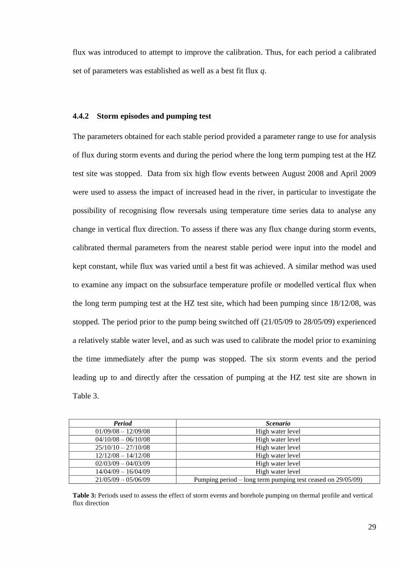
4.4.2 Storm episodes and pumping test

The parameters obtained for each stable period provided a parameter range to use for analysis

of flux during storm events and during the period where the long term pumping test at the HZ

test site was stopped. Data from six high flow events between August 2008 and April 2009

were used to assess the impact of increased head in the river, in particular to investigate the

possibility of recognising flow reversals using temperature time series data to analyse any

change in vertical flux direction. To assess if there was any flux change during storm events,

calibrated thermal parameters from the nearest stable period were input into the model and

kept constant, while flux was varied until a best fit was achieved. A similar method was used

to examine any impact on the subsurface temperature profile or modelled vertical flux when

the long term pumping test at the HZ test site, which had been pumping since 18/12/08, was

stopped. The period prior to the pump being switched off (21/05/09 to 28/05/09) experienced

a relatively stable water level, and as such was used to calibrate the model prior to examining

the time immediately after the pump was stopped. The six storm events and the period

leading up to and directly after the cessation of pumping at the HZ test site are shown in

Table 3.

Period Scenario

01/09/08 – 12/09/08 High water level

04/10/08 – 06/10/08 High water level

25/10/10 – 27/10/08 High water level

12/12/08 – 14/12/08 High water level

02/03/09 – 04/03/09 High water level

14/04/09 – 16/04/09 High water level

21/05/09 – 05/06/09 Pumping period – long term pumping test ceased on 29/05/09)

Table 3: Periods used to assess the effect of storm events and borehole pumping on thermal profile and vertical

flux direction

30

4.5 Results

4.5.1 Modelled flux during periods of stable river level

The calibrated thermal parameters and modelled vertical flux values for the selected stable

periods using the modified Ogata-Banks solution are shown in Table 4.

Period

Bulk

Volumetric

Heat Capacity

x106

(J m-3

K -1

)

Thermal

Conductivity

(W m-1

K -1

)

Thermal

Diffusivity

x10-6

(m2s

-1)

Vertical Flux

positive in

downward

direction x10-6

(ms-1

)

Average

RMSE from

Ogata-Banks

Model

24/08/08 – 30/08/08 2.25 4 1.78 -3.6 0.185

14/09/08 – 17/09/08 1.82 3 1.65 0.2 0.079

18/09/08 – 21/09/08 1.63 3 1.85 -2.1 0.107

11/10/08 – 15/10/08 1.75 2.5 1.43 -0.4 0.070

25/12/08 – 30/12/08 1.65 2.5 1.52 -0.5 0.128

01/01/09 – 07/01/09 1.26 1.6 1.27 0.6 0.133

09/01/09 – 11/01/09 2.3 1.9 0.83 -1.2 0.066

21/02/09 – 28/02/09 1.6 2.5 1.56 -0.4 0.056

29/03/09 – 07/04/09 1.6 2.3 1.44 -0.8 0.137

19/04/09 – 24/04/09 1.5 2.3 1.53 -1.1 0.172

Table 4: Calibrated flux and thermal parameter values for the modelled stable periods

During the calibration process there were several unusual or anomalous profiles at

certain depths which showed a considerable increase in residual error in comparison to other

depth profiles during that period. In these instances calibration was based on fitting a

simulated thermal profile to those depths which showed comparable behaviour. For several

periods (18/09/08 to 21/09/08, 09/01/09 to 11/01/09 and 21/05/09 to 24/05/09) the

temperature profile for 0.185m depth displayed noticeably larger than average residuals when

compared to the residual errors for other depths during these periods.

31

4.5.2 Modelled flux during storm episodes

The results from the modified Ogata-Banks model when used to analyse flux variation during

periods of increased flow are shown in Table 5.

Period

Approx.

Increase

in River

Head

(m)

Bulk

Volumetric

Heat

Capacity

x106

(J m-3

K -1

)

Thermal

Conductivity

(W m-1

K -1

)

Thermal

Diffusivity

x10-6

(m2s

-1)

Vertical

Flux

positive in

downward

direction

x10-6

(ms-1

)

Average

RMSE

from

Ogata-

Banks

Model

01/09/08 – 12/09/08 1.4 2.25 4 1.78 1.1 0.133

04/10/08 – 06/10/08 1.5 1.75 2.5 1.43 1.5 0.563

25/10/10 – 27/10/08 0.7 1.75 2.5 1.43 0.5 0.320

12/12/08 – 14/12/08 1.25 1.65 2.5 1.51 1.9 0.376

02/03/09 – 04/03/09 0.6 1.6 2.5 1.56 2.8 0.327

14/04/09 – 16/04/09 0.6 1.5 2.3 1.53 1.8 0.313

Table 5: Calibrated flux and thermal parameter values for the modelled storm flow periods

32

As can be seen from the modelled values of flux during high flow events, there is a

consistent indication that vertical flux direction is reversed. Downwards flux values seen in

Table 5 indicate substantial inflow to the hyporheic sediments but the residual errors from the

model during such storm episodes are also relatively high in comparison to those residuals

from modelled stable periods. These high residuals hint at something further with regards to

the system during flow reversals resulting from increased river levels, which cannot be

simulated by using such a simplified model. In particular, the period from 4/10/08 to

06/10/08 saw one of the highest increases in river level, an increase of approximately 1.5m.

Although the model indicates a change in flow, the residual errors in this model run were

substantially higher than the average errors, indicating that there is a limit within this model

for quantifying the impact of storm episodes and that the observed data is perhaps showing a

lateral component of flux and/or the thermal properties are being influence by flow reversal.

4.5.3 Modelled flux during and after pumping test

Calibrated thermal parameters and modelled flux values before and after the pumping test

was stopped using the modified Ogata-Banks solution are shown in Table 6.

Period

Bulk

Volumetric

Heat Capacity

x106

(J m-3

K -1

)

Thermal

Conductivity

(W m-1

K -1

)

Thermal

Diffusivity

x10-6

(m2s

-1)

Vertical Flux

positive in

downward

direction x10-6

(ms-1

)

Average

RMSE from

Ogata-Banks

Model

21/05/09 – 24/05/09 1.33 2.2 1.65 -0.26 0.131

25/05/28 – 28/05/09 1.65 2.5 1.52 -0.5 0.299

29/05/09* – 31/05/09 1.49 2.5 1.68 -0.8 0.208

01/06/09 – 05/06/09 1.49 2.5 1.68 -1.4 0.236

Table 6: Calibrated flux and thermal parameter values for the period before and after pumping of the extraction

borehole at the HZ test stopped. *indicates day when pump was stopped

33

The modelled flux values for the two modelled periods prior to pumping are relatively

similar. They indicate a small upward flux from the hyporheic sediments. However, after the

pump is switched off there is a steady but clear increase in vertical flux. Figure 9 shows a

graph of the squared residual errors for this entire period, showing the temperature profile

before and after pumping, using average thermal parameters and flux values for the two

modelled periods leading up to the pump being switched off. It can be seen from this that

when the pump is switched off on the 29/05/08, a definite increase in residual error in the

model starting on 29/05/08 and gradually increasing over the subsequent few days. The

model residuals from the two deepest levels of the temperature probe (0.285m and 0.395m)

show a continual increase in upwards flux over the days immediately after the pumping test, a

response which is not mirrored as strongly in the upper two temperature profiles (0.09m and

0.185m), although an increase in upwards flux relative to the period before pumping stopped

was estimated for all depths. The issues experienced in fitting thermal profiles at 0.09m and

0.185m with those observed at 0.285m and 0.395m might be as a result of the pumping test

being stopped, but the more evidence would be required to support this conclusion.

Furthermore, during the period modelled between 25/12/08 and 30/12/08, shortly after the

pump test was initiated, the residuals for depths of 0.185m, 0.285m and 0.395m showed a

better fit when the flux was decreased, with the uppermost profile, 0.09m, having a better fit

with a higher flux. The nature of this change in temperature profile and the flux estimates

derived from modelling seem to indicate that the deeper sediments are hydraulically

connected to the extraction borehole. It can also be argued that this is a sign of the hyporheic

outflow from the riverbed sediments being subdued at depth by the pumping of the extraction

borehole.

34

Figure 9: Graph of squared residuals from model run for period 21/05/09 to 05/06/09. Nb. Pump is switched off

on 29/05/09

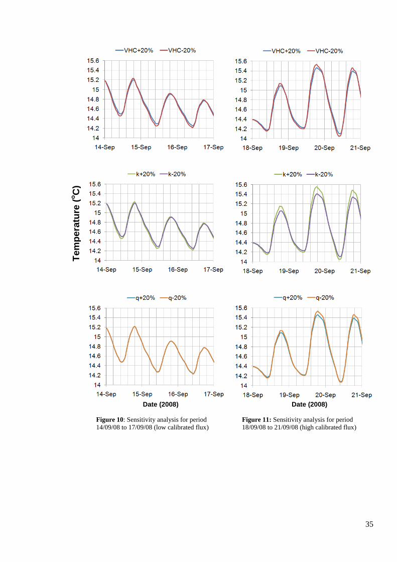
4.6 Sensitivity Analysis

Sensitivity analysis was carried out on the modified Ogata-Banks model by increasing and

decreasing each input parameter by 20%. Figures 10 and 11 show the relative sensitivity of

the model output to changes in magnitude of different parameters for periods where a low

vertical flux was estimated and a period where high vertical flux was estimated. Sensitivity

analysis was carried out on several modelled periods and indicated greatest sensitivity to

variations in thermal conductivity. Sensitivity analysis also highlighted the relationship

between uncertainty and the magnitude of estimated flux. In the case of lower fluxes the

sensitivity of the model to changes in thermal parameters and flux is noticeably reduced

relative to the sensitivity for higher fluxes. The implications of this are that for modelled flux

values which are relatively low, the uncertainty in the estimates for flux and thermal

properties is greatly increased. This is discussed further in Chapter 7.

Sq

ua

red

Res

idu

al

Date (2009)

35

Figure 10: Sensitivity analysis for period Figure 11: Sensitivity analysis for period

14/09/08 to 17/09/08 (low calibrated flux) 18/09/08 to 21/09/08 (high calibrated flux)

Tem

pera

ture

(oC

)

Date (2008) Date (2008)

36

5 NUMERICAL MODELLING

5.1 Introduction

In order to validate the modified Ogata-Banks semi-analytical model and assess its

applicability a numerical modelling exercise was undertaken. This involved conceptualising

and constructing a numerically based model using the data available from various

installations at the SWITCH test site. This approach would be used to examine selected

periods to serve as a validation for the flux estimates obtained for the same period using the

modified Ogata-Banks solution. The software chosen for numerical modelling was the United

States Geological Survey (USGS) variably saturated two-dimensional water and heat flow

program VS2DH (Healy & Ronan, 1996) which is combined with the graphical user interface

VS2DI* (Hsieh et al., 1999). This software package (herein referred to as VS2DI) can be used

to simulate flow, solute transport and heat transport in porous media with variable saturation.

The software setup involves: a graphical based pre-processor to construct the model domain

and input various required parameters; two numerical models available to solve for water,

solute and heat transport; and a postprocessor which provides visualisation of the results via a

simple animation using outputs at selected time steps (Healy, 2008). The model solves the

Richards equation (Richards, 1931) for flow and the advection-dispersion equation for solute

or heat transport using the finite-difference method. There are many software packages which

can be used for temperature time series analysis and thermal propagation through saturated

sediments. The VS2DI model was chosen for this study because it offered an easy to use

interface for model construction and did not demand extraneous volumes of information on

thermal and hydraulic properties. This package has been used in numerous studies looking at

* The VS2DI package which includes all the software described in Section 5.1 is publically available and can be

downloaded for free from the USGS website (http://www.usgs.gov)

37

heat flow in riverbed sediments and unconfined aquifers over the last two decades (see

Constantz & Stonestrom, 2003; Constantz, 2008; Healy, 2008) and as a tool for evaluating

analytical methods of calculating groundwater flux (Schmidt et al., 2008), adding weight to

its applicability here.

5.2 Conceptualisation and Construction

The conceptualised system which was used to construct the numerical model was simplified

to great extents in order to maintain the assumptions which govern the semi-analytical

modified Ogata-Banks solution. The system was assumed to be one-dimensional,

homogeneous and isotropic with constant and uniform thermal and hydraulic properties

during each model run. In order to validate the Ogata-Banks model the calibrated thermal

parameters used for the numerical model were kept the same as the calibrated values obtained

from the Ogata-Banks model for each given period. A range of hydraulic conductivity values

were used for the purposes of numerical modelling as there is large uncertainty in the

hydraulic conductivity of the sediments under investigation. The range used, 0.24 md-1

to

3.23 md-1

was given by Shepherd (2009) based on constant head permeameter tests

conducted on repacked sediments samples from the HZ test site (discussed further in Chapter

6). Other parameters which were required were taken from inbuilt generic values given as an

option by VS2DI when defining textural class and transport parameters. As the numerical

model was to calculate flux based on input head data and other input hydraulic parameters,

one of the main assumptions of the semi-analytical model, constant flux, could not hold.

However, the maximum and minimum flux values calculated by the numerical model over

the simulated time periods were acquired from the model output file and are given.

The dimensions of the model domain were defined based on the available data

hydraulic data from the SWITCH test site. The domain was constructed to simulate a one

38

dimensional vertical column through the subsurface. Time varying head and temperature data

was available for the river via the U/S and D/S divers, which were imported to form the top

boundary of the model. The VS2DI package allows the import of a time series of data for

head and/or temperature which allocates each imported value(s) to a user defined number of

recharge periods. This allowed the creation of a topmost boundary with variable head and

temperature. The bottom boundary was defined based on data which had been collected from

the borehole diver, which showed a near constant head and temperature throughout the year.

This boundary was set at 12m below the top boundary, using the diver position within the

borehole as an approximate guide, and the temperature and head data from the borehole diver

was imported in a similar fashion to the top boundary. No flow boundary conditions were

applied to each side of the model domain to maintain the one-dimensionality of the model.

The initial temperature conditions at each investigated depth were input in accordance

to those used in the modified Ogata-Banks model. Observation points were placed to match

the four depths of the observed riverbed temperature. The observation points facilitated the

output of temperature values for each time step at the designated depth, which could be

plotted against observed data for that depth after each model run using a simple spreadsheet.

Each recharge period was set at five minutes to match the frequency of the observed data,

except the first recharge period which was set to last 4 hours. This allowed the model to reach

a steady state of initial conditions before to reduce transient effects during the simulation.

The domain grid was defined to allow only vertical movement of water. Horizontally,

the mesh design allowed only one cell to cover the width of the domain. In the vertical

direction the grid design formed the finest mesh at the top of the model domain, which

became progressively coarser towards the bottom. The grid size for the zone under

investigation was set at 0.02m, to a depth 0.46m, which then coarsened downwards to 1m for

the lowermost 10m of the domain. The grid mesh size and time steps used for each recharge

39

period were well within the limits set by the Peclet and Courant numbers calculated for this

model. Furthermore, VS2DI allows the user to select from four options to specify the

relationship between pressure head and relative hydraulic conductivity (Healy & Ronan,

1996). In this study the preselected van Genuchten function was used to represent hydraulic

characteristic functions. Outputs selected for each model run included velocity, fluid balance

and energy balance.

5.3 Results

Output from the VS2DI model is provided at each time step, resulting in modelled values for

flux being output every five minutes. In order to provide a comparison to the modified Ogata-

Banks model, the range of vertical flux is given from the numerical model output for each

run. These flux estimates shown in Table 7, along with mass balances errors for fluid and

energy (heat). No head or temperature borehole data was available prior to 08/01/09 and as a

result the numerical modelling focussed on periods where there was enough data to define the

lower boundary condition over time.

Period

Ogata-Banks

Vertical Flux

positive in

downward

direction x10-6

(ms-1

)

VS2DI Vertical Flux positive

in upward direction x10-6

(ms-

1)

Total Mass Balance

Error from VS2DI

Simulation

For K =

0.24md-1

For K =

3.23md-1

Average

Fluid Error

(%)

Average

Energy

Error (%)

09/01/09 – 11/01/09 -1.2 0.31 – 0.39 4.22 – 5.30 0.00 6.55

21/02/09 – 28/02/09 -0.4 0.22 – 0.56 2.34 – 7.60 0.00 1.88

21/05/09 – 28/05/09 -0.26 to -0.5 0.26 – 0.42 3.37 - 5.75 0.00 0.48

Table 7: Vertical flux estimates from numerical modelling using VS2DI. Hydraulic conductivity values based

on estimates provided in Shepherd (2009)

40

6 HYDRAULIC DATA

6.1 Data Collection

Several hydraulic tests have been carried out at the site as part previous studies and the

ongoing SWITCH research. Data from manual head tests carried out between October 2007

and July 2008 were made available as a caparison tool for the flux measurements derived

from the models created during this study. The collection of this data is documented in

Cuthbert et al. (In Press). The closest available hydraulic data was taken from piezometer

installation P+005-1m, located approximately 0.5m upstream of the multilevel temperature

probe. This piezometer is installed to a depth of 49 cm into the riverbed. As the multilevel

temperature probe only monitors to a depth of 0.395m, the hydraulic calculations from

piezometer P+005-1m includes a 0.105m region not monitored by the temperature probe but

allowed a vertical gradient to be calculated over the entire depth interval it covers.

6.2 Freeze Coring

6.2.1 Introduction

In order to calculate flux manually based on Darcy’s Law using head data, hydraulic

conductivity values for the location around the temperature probe were required. As part of

this and other studies at the SWITCH HZ test site (Shepherd, 2009; Cuthbert et al., In Press)

a campaign of sediment coring was undertaken with the aim of achieving intact samples of

the upper region of the riverbed for analysis. During this sampling campaign, a core was

purposefully extracted from close to the multilevel temperature probe to gain an accurate

description of the sediment in that region of the riverbed. Through simple sediment analysis

41

these would allow estimates of hydraulic conductivity to be calculated. Field work was

carried out by Mark Cuthbert, Richard Johnson, Simon Shepherd and the author.

6.2.2 Methodology

The method of sediment coring was taken from (Stocker & Dudley Williams, 1972). This

method involved driving a hollow metal stake into the river bed and pouring liquid nitrogen

into the hollow stake, freezing the sediment onto the stake. The depth to which core could be

sampled were limited by the length of the metal stake and the water level in the river. Thus

sampling was undertaken after at least three days of little or no rainfall to ensure the river

level was low enough to work in safely and to retrieve adequate core lengths. Cores were

taken from 9 separate locations within the HZ test zone as indicated in Figure 4. The cores

were logged on site and samples taken for laboratory analysis. For the present study the

information from only one core (Freeze Core FC8) was used to provide estimates of

hydraulic conductivity and as a guide to the likely lithological properties in the substratum.

Freeze core FC 8 was taken as close to the multilevel temperature probe as possible, without

disturbing installation.

6.2.3 Results

The extracted core is shown in Figure 12. Sediment analysis by Shepherd (2009) provided

values for hydraulic conductivity at different depths which were used for manual flux

calculation and for numerical modelling, as stated in Section 5.2. A lithological description of

core FC8 is given in Appendix A. Full details of the method used and results obtained from

sediment analysis for all freeze cores extracted at the HZ test site can be found in Shepherd

(2009) and Cuthbert et al. (In Press).

42

Figure 12: Image showing freeze core FC8, shortly after

extraction, highlighting the sedimentary textures present in the

riverbed near temperature probe P+005-1T

6.3 Vertical Flux Derived from Hydraulic Data

A differential head was calculated using the difference between the water level in piezometer

P+005-1m and the water level of the river. A gradient was then calculated by dividing the

differential head by the depth from riverbed surface to the middle of the piezometer (Durand

et al., 2008). As the hydraulic gradient was measured at several times from October 2007 to

July 2008 by Durand et al. (2008), the maximum (0.19) and minimum (0.09) gradients will

be used for calculation. Hydraulic gradients were used to estimate vertical flux based on

Darcy’s Law. Hydraulic conductivity estimates for various depths (Shepherd, 2009) and

calculated flux values are shown in Table 8. These estimates were based on constant head

permeameter test on repacked sediment samples from various lithologically distinct layers in

core FC8, giving a range of values for hydraulic conductivity. . It should be noted that the

range given by Shepherd (2009) for this sediment core is in broad agreement with the values

obtained by slug test for the HZ test site by Durand et al. (2008) during initial research in

autumn 2007.

43

Depth (m) Hydraulic Conductivity (md-1) Calculated Vertical Flux range (ms-1)

0 - 0.15 Unknown Unknown

0.15 – 0.17 1.47 1.53E-06 – 3.23E-06

0.17 – 0.25 1.47 1.53E-06 – 3.23E-06

0.25 – 0.39 0.24 2.5E-07 – 5.28E-07

0.39 – 0.46 1.51 1.57E-06 – 3.32E-06

0.46 – 0.51 2.41 2.51E-06 – 5.30E-06

0.51 - 0.56 2.35 2.45E-06 – 5.17E-06

0.56 – 0.61 3.23 3.36E-06 – 710E-06

Table 8: Estimated flux values derived from Darcy based calculations. Nb. hydraulic gradients were measured

manually from 23/10/07 to 04/07/08 at piezometer P+005-1m. Range of measured vertical hydraulic gradient is

0.09 – 0.19.

44

7 DISCUSSION

7.1 Model Results

7.1.1 Comparison of derived vertical flux values

The present study aimed to provide estimates of water flux by applying temperature time

series analysis using data from the HZ test site on the River Tame, Birmingham. The semi-

analytical model created in this study was able to provide estimates of average flux over a

given time period based on direct comparison of observed and simulated data. Vertical flux

derived from the modified Ogata-Banks solution are within an order of magnitude range

compared to numerically derived values for the same periods of time, i.e. using identical

thermal parameters, initial conditions and surface temperature oscillations. For the period

between 21/05/09 and 28/05/09 the Ogata-Banks derived flux is at the lower end of the

numerically modelled range.

Estimates of vertical flux values from the modified Ogata-Banks solution also lie

within the range calculated from hydraulic gradients measured at the site. The role of

hydraulic conductivity is important when considering the results from the numerical model

and Darcian based equations. At higher flow rates hydraulic conductivity has a larger impact

on calculated flux than thermal parameters, with thermal properties becoming more important

for simulating flux at period of lower flow (Constantz & Stonestrom, 2003). The uncertainty

of hydraulic parameters for the SWITCH site has been discussed by several authors (Durand

et al., 2008; Shepherd, 2009; Cuthbert et al., In Press) and it is for this reason that a range of

hydraulic conductivity values were used in the numerical model and hydraulic calculations.

Although not providing complete validation for the modified Ogata-Banks method, the

45

similarity in flux ranges developed from all three sources of flux estimation do provide

encouragement for its use.

7.1.2 Temporal variability of flux

Analysis of the derived flux estimates indicates a general lowering of flux during the winter

months but this could a result of the relative stability of the river level during winter or may

be due to the effects of the long term pumping test which began in December 2008. The latter

suggestion is given support by the increase in flux values obtained from the days immediately

after the pump was switched off, suggesting that the flux rate was dampened by the ongoing

pumping at site, although this remains inconclusive. Modelled flux values from immediately

after the test do suggest that the thermal profile within the subsurface was altered by the

pumping test, although quantifying this effect would require a more complex analysis of the

system, and would likely profit from temperature time series data from other areas within this

reach.

7.1.3 Thermal properties and flux

Estimated values for heat capacity and thermal conductivity for the most part fall within the

range given by Lal (2005) and shown in Table 9. In analysing the calibrated thermal values

from the modified Ogata-Banks method a general decrease in volumetric heat capacity was

seen except for an anomalous value during the period from 09/01/09 to 11/01/09. A less

obvious decline in thermal diffusivity could be argued but given the uncertainties in the input

parameters this remains unconvincing. This is not mirrored in any obvious way by the

vertical flux values obtained from the modified Ogata-Banks solution with variable vertical

flux estimates being calculated throughout the year. The temporal heterogeneity of river bed

sediments is not as well documented as the spatial heterogeneity but studies have shown

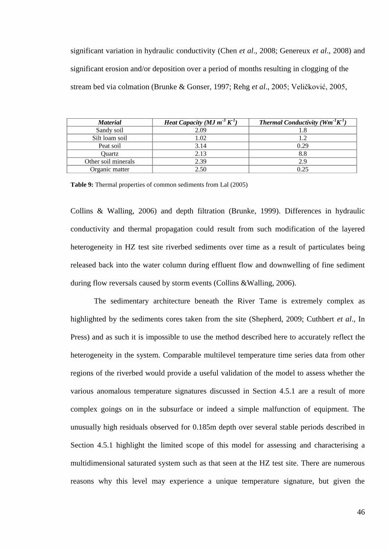
46

significant variation in hydraulic conductivity (Chen et al., 2008; Genereux et al., 2008) and

significant erosion and/or deposition over a period of months resulting in clogging of the

stream bed via colmation (Brunke & Gonser, 1997; Rehg et al., 2005; Veličković, 2005,

Table 9: Thermal properties of common sediments from Lal (2005)

Collins & Walling, 2006) and depth filtration (Brunke, 1999). Differences in hydraulic

conductivity and thermal propagation could result from such modification of the layered

heterogeneity in HZ test site riverbed sediments over time as a result of particulates being

released back into the water column during effluent flow and downwelling of fine sediment

during flow reversals caused by storm events (Collins &Walling, 2006).

The sedimentary architecture beneath the River Tame is extremely complex as

highlighted by the sediments cores taken from the site (Shepherd, 2009; Cuthbert et al., In

Press) and as such it is impossible to use the method described here to accurately reflect the

heterogeneity in the system. Comparable multilevel temperature time series data from other

regions of the riverbed would provide a useful validation of the model to assess whether the

various anomalous temperature signatures discussed in Section 4.5.1 are a result of more

complex goings on in the subsurface or indeed a simple malfunction of equipment. The

unusually high residuals observed for 0.185m depth over several stable periods described in

Section 4.5.1 highlight the limited scope of this model for assessing and characterising a

multidimensional saturated system such as that seen at the HZ test site. There are numerous

reasons why this level may experience a unique temperature signature, but given the

Material Heat Capacity (MJ m-3

K-1

) Thermal Conductivity (Wm-1

K-1

)

Sandy soil 2.09 1.8

Silt loam soil 1.02 1.2

Peat soil 3.14 0.29

Quartz 2.13 8.8

Other soil minerals 2.39 2.9

Organic matter 2.50 0.25

47

lithological description given by Shepherd (2009) is possible that the clay content of this

layer is exerting a noticeable effect on the average thermal properties of the sediment column.

However, it could also be explained by a simple thermistor malfunction.

The average results presented here over the entire 0.395m of investigation seem to

indicate certain influences at different depths which can ultimately not be accounted for by a

simple change in flux magnitude or thermal properties. The role of gas storage within the

sediments may also contribute to the variance in thermal parameters over time. Cuthbert et al.

(In Press) report significant volumes of gas stored within the riverbed, which seem to be

ubiquitous at the HZ Test site. Preliminary analysis suggests that the build up of gas within

the sediments may be attributed to denitrification within the hyporheic sediments, but work

on this began during the latter stages of this project and hence could not be incorporated into

this study. Although the effect of gas on thermal parameters is not considered here, if the

production of gas at the HZ test site is indeed significant and variable over time, then this

may also influence the subsurface thermal properties and may also aid in the explanation of

unusual thermal signature at different depths and different times.

Flux estimates using the modified Ogata-Banks method give confidence to identifying

flow reversals during high water levels events using temperature time series. In all modelled

storm scenarios the calibrated flux direction simulated influent conditions, contrasting to the

dominantly effluent conditions of the calibrated stable periods. This reach of the River Tame

is described as being generally effluent under ambient conditions (Durand et al., 2008). The

results from analytical modelling here support this description, at least for the section of the

streambed around the installed multilevel temperature probe.

48

7.2 Model Evaluation

The modified Ogata-Banks program written for this study has a number of simple advantages

in analysing temperature time series. Firstly, it is possible to gain an insight into the thermal

properties of the media and derive estimates of vertical flux without requiring excessive

information in regard to thermal and hydraulic properties. No hydraulic gradient or

conductivity data is required to utilise this method. As discussed in Constantz & Stonestrom

(2003) the greatest uncertainty when modelling seepage through sediments tends to come

from hydraulic parameters, which can vary over several orders of magnitude for a single

textural class. Thermal parameters however have a much smaller range when it comes to

sediment class and are almost independent of texture (Constantz & Stonestrom, 2003).

This method provides an easy to use analysis of vertical flux and thermal properties using

temperature time series data directly without the need for any pre-processing or complex

numerical computation.

Disadvantages of the model are generally linked to the simplified assumptions of

isotropy, homogeneous properties and average flux which govern the operation of the

modified Ogata-Banks solution. In particular, yielding of an averaged constant flux value

over a set time interval presents a distinct limit to the use of the modified Ogata-Banks

method, making this approach unsuitable for high resolution flux estimation. Other semi-

analytical methods are available which utilise the Stallman (1965) solution and can output a

time series of flux.

Methods such as that developed by Keery et al. (2007), can provide more detailed

information about flux change over time but these can require data to be processed before

being analysed with the analytical solution. The stepwise, modified Ogata-Banks approach

described here can be applied quickly to observed temperature time series and provide useful

information regarding the averaged flux and thermal behaviour of a saturated medium.

49

Moreover, during periods of low flow e.g. 14/09/08 to 18/09/08, the model uncertainty

increases considerably, resulting in questionable estimates for thermal parameters, flux

direction and magnitude. Stallman (1965) estimated that his solution would be useful for

calculating fluxes to a lower limit of around 2.3 x10-7

ms-1

using standard thermal properties

for porous sediments. Similarly, there is a lower threshold for calculating a flux value using

the modified Ogata-Banks Solution which would be on a comparable scale to the limit

suggested by Stallman (1965) based on sensitivity analysis (Section 4.6). In cases where

derived flux values were in the region of 3x10-7

ms-1

or lower, the sensitivity of the model to

incremental variation of thermal parameters and/or flux was relatively low, and as such the

estimates are delivered within an increased uncertainty.

For the purposes of this project, trial and error seemed an appropriate method from

which to calibrate the analytical model given the simplicity of the model setup. During early

calibration efforts a best fit simulated thermal profile for each depth was attempted but

proved excessively time consuming. In addition, the large dataset which was made available

for analysis meant that calibration of every time period would be impossible given the time

constraints of this project. In hindsight the development of an optimization code for use in

calibration may have been beneficial. It is important to note, however, that optimisation based

on residual error within the model may not have yielded the best simulated thermal profile

and any optimisation routines implemented would have to be subjected to manual visual

analysis to insure the best fit of observed and modelled thermal signatures.

The application of this model is best suited for broad spectrum analysis of average

flux and thermal properties, providing a quick and easy to execute method of temperature

time series analysis. More precise analysis would require the use of additional methods

which are likely to involve more complex implementation.

50

8 SUMMARY AND CONCLUSION

In recent times efforts to understand the interactions between rivers and groundwater have

been increased substantially. The international SWITCH (Sustainable Water (management)

Improves Tomorrows’ Cities’ Health) project is part of this global push to characterise the

exchange of surface and subsurface waters along river corridors. In collaboration with the

Environment Agency for England and Wales, the University of Birmingham has devised and

implemented a dense monitoring network, termed the Hyporheic Zone (HZ) test site, on a

reach of the River Tame, Birmingham, for the express purpose of achieving a greater

understanding of the nature of the hyporheic zone. As part of the River Tame SWITCH

project, high resolution temperature time series data has been collected from a multi-level

temperature probe for a period between August 2008 and June 2009.

In this separate study, temperature time series analysis using data from the SWITCH

site was used to derive estimates for flux and thermal properties of the hyporheic sediments at

the SWITCH HZ test site. Conventional methods of flux calculation based on Darcy’s Law

can be difficult to implement in such environments and a method was developed to directly

utilise the raw observed temperature time series data to provide estimate of thermal flux. The

semi-analytical method is based on a thermal analogue of the step function solution

developed by Ogata & Banks (1961) for the one dimensional advection-dispersion equation

used in solute transport calculations. This method employs a modified version of the Ogata-

Banks solution, with substitution of solute transport properties for equivalent thermal

properties. The principle of superposition is used in conjunction with the modified Ogata-

Banks step function to simulate the temperature profiles at depth within a column of saturated

sediment. A program written in Visual Basic (VB) language was used to solve the modified

Ogata-Banks equation. By varying the inputs for the program and calibrating using the

51

graphical output and residual error statistics it is possible to derive an estimate of vertical

flux, and other thermal properties.

The application of this method to the HZ test site temperature time series data yielded

flux estimates within an order of magnitude range of estimates derived from Darcian based

flux calculations based on manual piezometer data gathered by the University of Birmingham

during fieldwork at the HZ test site. To further test the validity of the modified Ogata-Banks

solution for estimating vertical flux, a one dimensional numerical model was constructed

using the USGS software package VS2DI which is capable of modelling flow solute and

energy transport in variably saturated media. Estimated thermal parameters derived from the

modified Ogata-Banks model were input into the numerical model along with data from

borehole and river divers installed at the HZ test site and run over three identical periods

which had been modelled using the semi-analytical method. The estimates of flux from the

modified Ogata-Banks model fell within the range computed by the numerical model.

Results from the modified Ogata-Banks model indicate consistent upwards flux of

varying magnitude during periods of stable river level. Flow reversals are also indicated by

vertical flux estimates derived from periods of increased river head. It has also been shown

that the influence of borehole testing can seen in the subsurface temperature profile, but the

exact magnitude of this influence is inconclusive.

The method developed here can be easily and directly applied to temperature time

series data and provides useful averaged estimates of vertical flux and thermal parameters.

Although not suitable for complex and high resolution time series analysis, the application of

this method can provide useful information regarding water movement and temperature

propagation within a saturated medium without the need to define uncertain hydraulic

parameters or perform complex pre-processing of data.

52

REFERENCES

Bouyoucos, G., 1915. Effects of temperature on some of the most important physical process

in soils, Mich. Coll. Agric. Tech. Bull., 24, 1 – 63.

Bredehoeft, J.D.,& Papadopolus, I.S., 1965. Rates of vertical groundwater movement

estimated from the Earth’s thermal profile. Water Resources Research 1 (2), 325–328.

Brunke, M., 1999. Colmation and depth filtration within streambeds. Retention of particles in

hyporheic interstices. International Review of Hydrobiology, 84, 99-117.

Brunke, M., & Gonser, T., 1997. Ecological significance of exchange processes between

rivers and groundwater. Freshwater Biology, 37, 1-33.

Chen, X., Burback, M., & Cheng, C., 2008. Electrical and hydraulic vertical variability in

channel sediments and its effects on streamflow depletion due to groundwater

extraction. Journal of Hydrology, 352, 250– 266.

Conant Jr., B., 2004. Delineating and quantifying ground water discharge zones using

streambed temperatures. Ground Water, 42 (2), 243–257.

Constantz, J., & Stonestrom, D.A., 2003. Heat as a tracer of water movement near streams,

In: Stonestrom, D.A., Constantz, J. (Eds.), Heat as a Tool for Studying the Movement

of Ground Water Near Streams, US Geological Survey Circular 1260. US Geological

Survey, Reston, VA, pp. 1–6.

Constantz, J., 2008. Heat as a tracer to determine streambed water exchanges, Water

Resources Researc,,44, Article Number: W00D10

Cuthbert, M., Aller, M.F., Durand, V., Greswell, R.B., Mackay, R., & Rivett, M.O., In Press.

River Tame Hyporheic Zone SWITCH Test Site – Interim Data Report, Environment

Agency, UK

Durand, V., Rivett, M.O., Mackay, R., Aller, M.F. & Greswell, R.B., 2008. Development

of the Hyporheic Zone Test Site and Experimental Design. SWITCH progress report

.

E.A., Environment Agency, 2002. The Water Framework Directive: Guiding principles on

the technical requirements, Environment Agency, UK.

Ellis, P.A., Mackay, R., & Rivett, M.O., 2007. Quantifying urban river-aquifer fluid

exchange processes: A multi-scale problem. Journal of Contaminant Hydrology, 91,

58-80.

Ellis, P.A., & Rivett, M.O.,2007. Assessing the impact of VOC-contaminated

groundwater on surface water at the city scale. Journal of Contaminant Hydrology,

91, 107-127.

53

Essaid, H.I., Zamora, C.M., McCarthy, K.A., Vogel, J.R., & Wilson, J.T., 2008. Using heat to

characterize streambed water flux variability in four stream reaches, Journal of

Environmental Quality, 37, 1010-1023

European Commission, 2000. Directive 2000/60/EC of the European Parliament and of the

Council establishing a framework for Community action in the field of water policy.

Official Journal of the European Community L327, 1–72.

Genereux, D.P., Leahy, S., Mitasova, H., Kennedy, C.D., & Corbett, D.R., 2008. Spatial and

temporal variability of streambed hydraulic conductivity in West Bear Creek, North

Carolina, USA. Journal of Hydrology, 358, 332– 353.

Hatch, C.E., Fisher, A.T., Revenaugh, J.S., Constantz, J., & Ruehl, C., 2006. Quantifying

surface water–groundwater interactions using time series analysis of streambed t

hermal records: method development. Water Resources Research, 42 (10), W10410.

Healy, R.W., & Ronan, A.D. 1996. Documentation of the Computer Program VS2DH for

Simulation of Energy Transport in Variably Saturated Porous Media – Modification

of the US Geological Survey’s Computer Program VS2DT. Reston, Virginia, USGS.

US Geological Survey Water-Resources Investigation Report 96-4230.

Healy, R.W., 2008. Simulating water, solute and heat transport in the subsurface with the

VS2DI software package, Vadose Zone Journal, 7 (2), 632–639

Hiscock, K., 2004. Hydrogeology Principles and Practice, Wiley-Blackwell, 408 pages

Hsieh, P.A., W. Wingle, & R.W. Healy. 1999. VS2DI: A graphical software package

for simulating fluid flow and solute or energy transport in variably saturated porous

media. Water-Resour. Invest. Rep. 99-4130. USGS, Reston, VA.

Keery, J., Binley, A., Crook, N., Jonathan W.N. Smith, & J.W.N., 2007. Temporal and spatial

variability of groundwater–surface water fluxes: Development and application of an

analytical method using temperature time series, Journal of Hydrology, 336, 1– 16

Lapham, W.W., 1989. Use of temperature profiles beneath streams to determine rates of

vertical ground-water flow and vertical hydraulic conductivity. US Geological Survey

Water Supply Paper 2337, US Geological Survey, Denver, CO, 35pp.

Lal, R.(Ed), 2005. Encyclopedia of Soil Science, Volume 1, Marcel Dekker Ltd.

Ogata, A. & Banks, R.B., 1961. A solution of the differential equation of longitudinal

dispersion in porous media. U.S. Geol. Surv. Prof. Papers, 411-A.

Poole, G.C., O’Daniel, S.J., Jones, K.L., Woessner, W.W., Bernhardt, E.S., Helton, A.M.,

Stanford, J.A., Boer, B.R., and Beechie, T.J., 2008. Hydrologic spiralling: the role of

multiple interactive flow paths in stream ecosystems. River Research and

Applications, 24, 1018-1031

Rehg, K.J., Packman, A.I., & Ren, J., 2005. Effects of suspended sediment characteristics and

bed sediment transport on stream- bed clogging. Hydrological Processes, 19, 413–

427.

54

Richards, L.A. 1931. Capillary conduction of liquids through porous mediums. Physics, 1,

318–333.

Rivett, M.O, Ellis, P., Greswell, R.B., Ward, R.S., Roche, R.S, Cleverly, M., Walker, C.,

Conran, D., Fitzgerald, P.J., Willcox, T., & Dowle, J., 2008. Cost-effective mini

drive-point piezometers and multilevel samplers for monitoring the hyporheic zone,

Quarterly Journal of Engineering Geology & Hydrogeology, 41 (1), 49-60.

Scmidt, C., Conant Jr., B., Bayer-Raich, M., & Schirmer, M., 2007. Evaluation and field-

scale application of an analytical method to quantify groundwater discharge using

mapped streambed temperatures, Journal of Hydrology, 347, 292-307.

Shepherd, S., 2009. Hydraulic controls on water quality variations: The River Tame

Hyporheic zone SWITCH urban test site, MSc. Thesis, School of Geography, Earth &

Environmental Sciences, University of Birmingham, UK.

Silliman SE, & Booth DF, 1993. Analysis of time-series measurements of sediment

temperature for identification of gaining vs. losing portions of Juday Creek, Indiana.

Journal of Hydrology. 146, 131-148

Silliman, S. E., Ramirez, J.,& McCabe, R.L., 1995. Quantifying downflow through creek

sediments using temperature time series: one-dimensional solution incorporating

measured surface temperature, Journal of Hydrology 167, 99-119

Smith, J.W.N., Bonell, M., & Gibert, J., 2008. Groundwater-surface water interactions,

nutrient fluxes and ecological response in river corridors: Translating science into

effective environmental management. Hydrological Processes, 22, 151-157.

Sophocleous, M., 2002. Interactions between ground and surface water: the state of the

science. Hydrogeology Journal, 10, 52–67.

Stallman, R.W., 1965. Steady one-dimensional fluid flow in a semiinfinite porous medium

with sinusoidal surface temperature. Journal of Geophysical Research, 70 (12), 2821–

2827.

Stocker Z.S.J. & Dudley Williams, D. 1972. A Freezing Core Method for Describing the

Vertical Distribution of Sediments in a Streambed. Limnology and Oceanography, 17

(1) , pp. 136-138.

Suzuki, S., 1960. Percolation measurements based on heat flow through soil with special

reference to paddy fields. Journal of Geophysical Research, 65 (9): 2883-2885.

Turcotte, D.L., & Schubert, G., 1982. Geodynamics: Applications of Continuum Physics to

Geological Problems. John Wiley & Sons, New York

Veličković, B., 2005. Colmation as one of the processes in interaction between groundwater

and surface water. Architecture and Civil Engineering, 3, (2), 165 – 172.

55

Winter, T.C., Harvey, J.W., Franke,O.L., & Alley W.M., 1998. Ground water and surface

water – a single resource. US Geological Survey Circular 1139

Woessner, W.W., 2000. Stream and fluvial plain groundwater interactions: rescaling

hydrogeologic thought. Ground Water 38 (3), 423–429.

56

APPENDIX A

Freeze Core FC8

Sample date: 26/06/09

Core collected by M. Cuthbert, M.B. Hendrie, S. Shepherd

Logged by S. Shepherd

Location: 35cm toward borehole side bank from piezometer P+005-1p (box1)

Depth (m) Description Hydraulic Conductivity (md-1

)

0 - 0.15 sediment lost during extraction unknown

0.15 – 0.17 Dark brown organic soil; angular and

rounded pebbles (0.3 – 1cm) 1.47

0.17 – 0.25 Grey brown clayey sand; pebbles, sub-

rounded (0.3 – 1cm) 1.47

0.25 – 0.39 Grey brown clayey sand; pebbles and

cobbles, sub-rounded (0.3 –7cm) 0.24

0.39 – 0.61

Orange-brown sand, uniform, fine to

medium grained, abundant quartz, some

mica 1.51 - 3.23

Table 10: Log and data taken of freeze core FC8. Hydraulic conductivity values were derived from a constant

head permeameter teat on repacked sediments samples. (Modified from Shepherd, 2009)

57

LIST OF ELECTRONIC APPENDICES

Electronic Appendix A (on CD-ROM)

A copy of the data collated for the purposes of this studied is provided

Electronic Appendix B (on CD-ROM)

A version of the modified Ogata-Banks model developed and used in this study is provided,

with instructions for use.