ASSESSMENT AND MITIGATION OF LIQUEFACTION HAZARDS TO

BRIDGE APPROACH EMBANKMENTS IN OREGON

Final Report

SPR 361

by

Dr. Stephen E. Dickenson Associate Professor

and Nason J. McCullough

Mark G. Barkau Bryan J. Wavra

Graduate Research Assistants Dept. of Civil Construction and Environmental Engineering

Oregon State University Corvallis, OR 97331

for

Oregon Department of Transportation Research Group

200 Hawthorne Ave. SE Salem, OR 97301-5192

and

Federal Highway Administration

Washington, D.C. 20590

November 2002

Technical Report Documentation Page 1. Report No.

FHWA-OR-RD-03-04

2. Government Accession No.

3. Recipient’s Catalog No.

5. Report Date November 2002

4. Title and Subtitle

Assessment and Mitigation of Liquefaction Hazards to Bridge Approach Embankments in Oregon 6. Performing Organization Code

7. Author(s) Stephen E. Dickenson, Nason J. McCullough, Mark G. Barkau, and Bryan J. Wavra

8. Performing Organization Report No. 10. Work Unit No. (TRAIS)

9. Performing Organization Name and Address

Oregon State University Department of Civil, Construction, and Environmental Engineering 202 Apperson Hall Corvallis, Oregon 97331

Contract or Grant No. K5010A

SPR 361 13. Type of Report and Period Covered Final Report 1994- 2001

12. Sponsoring Agency Name and Address

Oregon Department of Transportation Research Group and Federal Highway Administration 200 Hawthorne Ave SE Washington, D.C. 20590 Salem, Oregon 97301-5192 14. Sponsoring Agency Code 15. Supplementary Notes 16. Abstract

The seismic performance of bridge structures and appurtenant components (i.e., approach spans, abutments and foundations) has been well documented following recent earthquakes worldwide. This experience demonstrates that bridges are highly vulnerable to earthquake-induced damages and loss of serviceability. These damages are commonly due to soil liquefaction and the associated impact of ground failures on abutments and pile foundations.

Current design methods for evaluating permanent, seismically-induced deformations of earth structures are based on rigid body, limit equilibrium and “sliding-block” procedures that are poorly suited for modeling soil liquefaction and establishing the pattern of embankment-abutment-foundation deformations. Recent advances in the seismic design of bridges have addressed some of the limitations of the current design procedures; however practice-oriented methods for estimating permanent deformations at sites that contain liquefiable soils and/or where soil improvement strategies have been employed to mitigate liquefaction hazards are still at an early stage of development. In Oregon, the evaluation of soil liquefaction and abutment performance are complicated by the rather unique seismo-tectonic setting and the prevalence of silty soils along the primary transportation corridors in the Portland/Willamette Valley region and along the Columbia River.

This study has focused on numerical dynamic, effective stress modeling to determine the seismic performance of sloping abutments and the effectiveness of soil improvement for reducing permanent ground deformations. Recommendations are provided for evaluating the dynamic behavior of regional silty soils, the application of soil improvement at bridge sites, and comparisons have been made between the deformations computed using the advanced numerical model and the rigid-block methods used in practice. The results have been presented in the form of design charts, where possible, that can be readily used by design engineers in preliminary design and incorporated into the ODOT Liquefaction Mitigation Policy. This study has demonstrated the utility, and limitations, of soil improvement solely by densification techniques. In some cases soil densification techniques for mitigating seismic hazards may not be adequate in limiting deformations to allowable limits, indicating that other methods of soil improvement (e.g., cementation, stone columns, drainage) or structural improvements may also be required.

17. Key Words liquefaction, bridge abutment, ground failure, soil improvement, seismic design

18. Distribution Statement Copies available from NTIS.

19. Security Classif. (of this report) Unclassified

20. Security Classif. (of this page) Unclassified

20. No. of Pages

22. Price

Technical Report Form DOT F 1700.7 (8-72) Reproduction of completed page authorized

i

ACKNOWLEDGMENTS

The authors would like to express their sincere gratitude to those individuals who provided valuable assistance throughout the duration of this investigation. Significant contributions were made during several key stages of the project.

The silt liquefaction studies reported herein are based in large part on the collection of data contained in numerous personal and proprietary files. This portion of the report has been enhanced by the significant contributions of regional data provided by Mr. Jason Brown of GeoEngineers (formerly Graduate Research Assistant at OSU), Mr. Andrew Vessely of Cornforth Consultants, and Dr. Michael Riemer of the Department of Civil and Environmental Engineering at the University of California, Berkeley. We are grateful to Dr. Wolfgang Roth of URS Corporation (Dames & Moore) and Mr. Douglas Schwarm of GeoEngineers for their assistance with the numerical modeling and for providing valuable insights on the pore pressure generation routines.

Reference material was provided from the personal files of several individuals. We are indebted to the following people: Yumei Wang of the Oregon Department of Geology and Mineral Industries, Mr. Ian Austin of URS Corporation (Dames & Moore) for sharing photographs from Kobe, Japan, and Professor Masanori Hamada of Waseda University, Tokyo, Japan for providing a copy of his outstanding report on liquefaction and ground displacements resulting from the 1995 Kobe Earthquake.

Project guidance and peer review was provided by the Technical Advisory Committee (TAC), which was convened by the Oregon Department of Transportation (ODOT). Active committee members included: Messrs. Jan Six and Dave Vournas (Geo-Hydro Section), Mr. Bruce Johnson of the Federal Highway Administration, and Ms. Elizabeth Hunt of the Research Group at ODOT. These TAC members provided reference material, ODOT bridge foundation plans and geotechnical reports, and thoughtful advice throughout the project. The TAC was assisted in the review of the final project report by Ms. Sarah Skeen of the Federal Highway Administration. This assistance is greatly appreciated. Finally, we are especially grateful to Ms. Elizabeth Hunt for her valuable assistance with the administration of the research project and organization of the TAC.

iii

DISCLAIMER

This document is disseminated under the sponsorship of the Oregon Department of Transportation and the United States Department of Transportation in the interest of information exchange. The State of Oregon and the United States Government assume no liability of its contents or use thereof.

The contents of this report reflect the views of the author(s) who are solely responsible for the facts and accuracy of the data presented herein. The contents do not necessarily reflect the official policies of the Oregon Department of Transportation or the United States Department of Transportation. The State of Oregon and the United States Government do not endorse products of manufacturers. Trademarks or manufacturers’ names appear herein only because they are considered essential to the object of this document.

This report does not constitute a standard, specification, or regulation.

iv

ASSESSMENT AND MITIGATION OF LIQUEFACTION HAZARDS TO BRIDGE APPROACH EMBANKMENTS IN OREGON

TABLE OF CONTENTS

1.0 INTRODUCTION................................................................................................................. 1 1.1 BACKGROUND.................................................................................................................. 1 1.2 STATEMENT OF OBJECTIVES AND SCOPE OF WORK ......................................................... 3

1.2.1 Objectives.................................................................................................................... 3 1.2.2 Scope of Work ............................................................................................................. 5 1.2.3 Report Organization ................................................................................................... 6

2.0 OVERVIEW OF LIQUEFACTION-INDUCED DAMAGE TO BRIDGE APPROACH EMBANKMENTS AND FOUNDATIONS ............................................ 9

2.1 INTRODUCTION ................................................................................................................ 9 2.2 LIQUEFACTION-INDUCED BRIDGE DAMAGE .................................................................. 10 2.3 OVERVIEW OF HISTORIC DAMAGE TO BRIDGE FOUNDATIONS ....................................... 12

2.3.1 1964 Alaska Earthquake ........................................................................................... 12 2.3.2 1964 Niigata Earthquake.......................................................................................... 19 2.3.3 1989 Loma Prieta Earthquake.................................................................................. 23 2.3.4 1991 Costa Rica Earthquake .................................................................................... 28 2.3.5 1995 Hyogo-Ken-Nanbu (Kobe) Earthquake ........................................................... 30

2.4 CONCLUSIONS................................................................................................................ 37

3.0 EVALUATION OF LIQUEFACTION SUSCEPTIBILITY: IN SITU AND LABORATORY PROCEDURES ................................................................................. 39

3.1 LIQUEFACTION HAZARD EVALUATION .......................................................................... 39 3.2 PRELIMINARY SITE INVESTIGATION ............................................................................... 41

3.2.1 Potentially Liquefiable Soil Types ............................................................................ 41 3.2.2 Saturation Requirement ............................................................................................ 44 3.2.3 Geometry of Potentially Liquefiable Deposits.......................................................... 44

3.3 QUANTITATIVE EVALUATION OF LIQUEFACTION RESISTANCE: OVERVIEW OF EXISTING PROCEDURES .......................................................................................... 45

3.3.1 Empirical Methods.................................................................................................... 45 3.3.2 Analytical / Physical Modeling Methods and Approaches ....................................... 45 3.3.3 Approximate Methods ............................................................................................... 46

3.4 LIQUEFACTION RESISTANCE: EMPIRICAL METHODS BASED ON IN SITU PENETRATION RESISTANCE .................................................................................... 49

3.4.1 Earthquake-Induced Cyclic Stress Ratios................................................................. 50 3.4.2 In Situ Liquefaction Resistance – The Cyclic Resistance Ratio................................ 53 3.4.3 Factor of Safety and Degree of Cyclic Pore Pressure Generation .......................... 72

4.0 POST-LIQUEFACTION SOIL BEHAVIOR .................................................................. 75 4.1 INTRODUCTION .............................................................................................................. 75 4.2 POST-CYCLIC STRENGTH OF SANDS AND SILTS ............................................................. 75

v

4.2.1 Partial Excess Pore Pressure Generation (1.0 < FSL <1.4) .................................... 76 4.2.2 Full Liquefaction (FSL < 1) ...................................................................................... 76

4.3 INTRODUCTION TO MODES OF FAILURE ......................................................................... 82 4.3.1 Global Instability and Flow Failures ....................................................................... 82 4.3.2 Localized Liquefaction Hazard and Lateral Spreading ........................................... 83 4.3.3 Excessive Deformation of Retaining Structures and Abutments............................... 84

4.4 EMPIRICAL METHODS FOR ESTIMATING LATERAL SPREAD DISPLACEMENT.................. 85 4.4.1 The Liquefaction Severity Index................................................................................ 85 4.4.2 Lateral Ground Displacement from Regression Analysis ........................................ 87 4.4.3 EPOLLS Model for Lateral Spread Displacement ................................................... 89

4.5 ANALYTICAL METHODS FOR ESTIMATING LATERAL SPREAD DISPLACEMENT .............. 89 4.5.1 Newmark Sliding Block Model.................................................................................. 89 4.5.2 Advanced Numerical Modeling of Slopes ................................................................. 94

4.6 EVALUATION OF GROUND SETTLEMENTS FOLLOWING CYCLIC LOADING ..................... 95 4.7 LATERAL SPREADING AND PILE FOUNDATION RESPONSE: DESIGN CONSIDERATIONS .. 98

4.7.1 Pile Failure Modes ................................................................................................... 99

5.0 MITIGATION OF LIQUEFACTION HAZARDS ....................................................... 101 5.1 INTRODUCTION ............................................................................................................ 101 5.2 TECHNIQUES FOR MITIGATING LIQUEFACTION HAZARDS............................................ 101 5.3 DESIGN OF SOIL MITIGATION....................................................................................... 104 5.4 DESIGN FOR THE AREA OF SOIL MITIGATION............................................................... 105

6.0 NUMERICAL MODELING............................................................................................ 109 6.1 CONSTITUTIVE SOIL MODEL ........................................................................................ 110 6.2 PORE PRESSURE GENERATION ..................................................................................... 111 6.3 GENERAL MODELING PARAMETERS............................................................................. 112

6.3.1 Modeling of Soil Elements ...................................................................................... 112 6.3.2 Modeling of the Earthquake Motion ....................................................................... 113 6.3.3 Modeling of the Water ............................................................................................ 114 6.3.4 Boundary Conditions .............................................................................................. 114

6.4 VALIDATION OF NUMERICAL MODEL .......................................................................... 114

7.0 DEFORMATION ANALYSIS OF EMBANKMENTS................................................. 117 7.1 INTRODUCTION ............................................................................................................ 117 7.2 ANALYSIS METHODS FOR ESTIMATING DISPLACEMENTS............................................. 118

7.2.1 Introduction............................................................................................................. 118 7.2.2 Pseudostatic Methods of Analysis for Competent Soils.......................................... 118 7.2.3 Analysis of the “Post-Earthquake” Factor of Safety for Slopes............................. 119 7.2.4 Limited Deformation Analysis ................................................................................ 120 7.2.5 Advanced Numerical Modeling............................................................................... 124

7.3 PARAMETRIC STUDY.................................................................................................... 125 7.3.1 Embankment Geometry........................................................................................... 127 7.3.2 Material Properties................................................................................................. 127 7.3.3 Ground Motions ...................................................................................................... 127

7.4 RESULTS OF PARAMETRIC STUDY................................................................................ 128 7.5 CONCLUSIONS.............................................................................................................. 136

vi

8.0 HAZARD EVALUATION AND DEVELOPMENT OF MITIGATION STRATEGIES – EXAMPLE PROBLEM.................................................................. 139

8.1 INTRODUCTION ............................................................................................................ 139 8.1.1 Geotechnical Site Characterization........................................................................ 140 8.1.2 Analyses of Seepage and Static Stability of Riverfront Slopes ............................... 143 8.1.3 Liquefaction Hazard Analyses ................................................................................ 143 8.1.4 Seismic Performance Evaluation............................................................................ 143

8.2 REGIONAL NATURAL HAZARDS................................................................................... 144 8.2.1 Flood Hazard .......................................................................................................... 144 8.2.2 Seismic Hazard ....................................................................................................... 145

8.3 GEOTECHNICAL FIELD INVESTIGATION........................................................................ 149 8.3.1 Subsurface Conditions ............................................................................................ 149

8.4 GROUND SHAKING EVALUATION ................................................................................. 149 8.4.1 Summary of Recent Seismic Hazard Investigations................................................ 151 8.4.2 Subduction Zone Bedrock Motions ......................................................................... 152 8.4.3 Crustal Bedrock Ground Motions........................................................................... 155

8.5 DYNAMIC SOIL RESPONSE ANALYSES ......................................................................... 155 8.5.1 Dynamic Response Analysis Method, SHAKE91.................................................... 157 8.5.2 Results of the Dynamic Soil Response Analysis...................................................... 160

8.6 LIQUEFACTION ANALYSIS............................................................................................ 163 8.6.1 Determination of the Cyclic Stress Ratio................................................................ 163 8.6.2 Determination of the Cyclic Resistance Ratio ........................................................ 163

8.7 EVALUATION OF INITIATION OF LIQUEFACTION........................................................... 168 8.8 DETERMINATION OF CYCLIC SHEAR STRENGTH .......................................................... 168

8.8.1 Partial Excess Pore Pressure Generation (1.0 < FSL <1.4) .................................. 168 8.8.2 Liquefied State (FSL < 1) ........................................................................................ 171

8.9 DEFORMATION ANALYSES........................................................................................... 172 8.9.1 Newmark Sliding Block Analyses............................................................................ 173 8.9.2 Simplified Chart-Based Displacement Estimates ................................................... 176 8.9.3 Numerical Dynamic Analysis.................................................................................. 177 8.9.4 Comparison of the Methods .................................................................................... 181 8.9.5 Application of Soil Improvement ............................................................................ 183

8.10 SUMMARY AND CONCLUSIONS..................................................................................... 186 8.11 LIMITATIONS AND RECOMMENDATIONS FOR FUTURE WORK....................................... 187

9.0 SUMMARY AND CONCLUSIONS ............................................................................... 189 9.1 RECOMMENDATIONS PERTINENTS TO LIQUEFACTION HAZARD EVALUATIONS

IN OREGON ........................................................................................................... 190 9.2 GENERAL RECOMMENDATIONS FOR FUTURE WORK.................................................... 191

10.0 REFERENCES.................................................................................................................. 193

vii

LIST OF TABLES

Table 3.1: Estimated Susceptibility of Sedimentary Deposits to Liquefaction during Strong Seismic Shaking....................................................................................................................................43

Table 3.2: Criteria Used in Compiling Liquefaction Susceptibility Map for the San Fernando Valley, California ..............................................................................................................................................44

Table 3.3: A Microzonation Procedure Based on Topography ............................................................................44 Table 3.4: Advantages and Disadvantages of the SPT and CPT for the Assessment of Liquefaction

Resistance..............................................................................................................................................49 Table 3.5: Proposed Simplified Site Classification System ...................................................................................52 Table 3.6: Boundaries of Soil Behavior Type.........................................................................................................62 Table 3.7: Values of CSR Correction Factor, c) ....................................................................................................66 Table 3.8: Influence of OCR on the Cyclic Stress Ratio Required to Cause Liquefaction and Large

Strains in Silt Specimens......................................................................................................................69 Table 4.1: Recommended Fines Correction for Estimation of Residual Undrained Strength...........................80 Table 4.2: Recommended Fines Correction for Estimation of Residual Undrained Strength...........................81 Table 4.3: Ranges of Input Values for Independent Variables for Which Predicted Results are

Verified by Case History Observations ..............................................................................................88 Table 5.1: Liquefaction Remediation Measures ..................................................................................................102 Table 6.1: Comparison of FLAC and Finite Element Numerical Programs .....................................................110 Table 7.1: Material Properties Used in Parametric Study..................................................................................125 Table 7.2: Earthquake Motions Used in the Parametric Study..........................................................................128 Table 7.4: Summary of FLAC Displacements......................................................................................................132 Table 8.1: Critical Flood Elevations for the Columbia River Near the Portland International Airport ........144 Table 8.2: Conversion Table for Various Data ....................................................................................................145 Table 8.3: Comparison of Recommended PGA Values for the Site ...................................................................151 Table 8.4: Attenuation Relationship Input Parameters with the Resulting PGArock Values............................153 Table 8.5: Selected Acceleration Time Histories..................................................................................................154 Table 8.6: Summary of PGA values ......................................................................................................................163 Table 8.7: Cyclic Resistance Ratio (CRR) from Lab Test Data for Normally Consolidated, Silty Soils ........165 Table 8.8: Magnitude Scaling Factors, MSF ........................................................................................................166 Table 8.9: Fines Content Values Estimated for Residual Undrained Shear Strength Analyses......................172 Table 8.10: Peak Horizontal Acceleration Values for the Scenario Earthquakes.............................................175 Table 8.11: Critical Acceleration (ay) Values for Residual Strength Conditions ..............................................175 Table 8.12: Deformation Results from Newmark Analyses Using Residual Strength Values .........................176 Table 8.13: Deformation Results from the Makdisi-Seed Method Using Residual Strength Values ..............176 Table 8.14: Deformation Results from the Bracketed Intensity Method Using Residual Strength Values ....177 Table 8.15: Deformation Results from the Parametric Study Outlined in Chapter 7. .....................................177 Table 8.16: Soil Properties Used in the Numerical Model. .................................................................................178 Table 8.17: Deformation Results from Numerical Model Analyses with River Elev. at 2.1 m (7 ft) ...............180 Table 8.18: Deformation Results from Numerical Model Analyses with River Elev. at 8.8 m (29 ft) .............180 Table 8.19: Deformation Results from Numerical Model Analyses with River Elevation at the Crest ..........181 Table 8.20: Riverward Deformation Results Comparison for the Earthquake Magnitude 8.5 Analyses.......182 Table 8.21: Comparison of Predicted Maximum Levee Displacements With and Without Soil

Improvement at the 100 yr flood stage. ............................................................................................186

viii

LIST OF FIGURES

Figure 1.1: ODOT’s Liquefaction Mitigation Procedure..............................................................................................4 Figure 2.1: Salinas River Bridge Damage ..................................................................................................................11 Figure 2.2: Area of Damage of 1964 Alaska Earthquake ...........................................................................................13 Figure 2.3: Bridge 596, Resurrection River. Centerline Section Looking Upstream (Natural Scale) .......................13 Figure 2.4: Bridge 598, Resurrection River. Centerline Section Looking Upstream (Natural Scale) .......................14 Figure 2.5: Bridge 596................................................................................................................................................14 Figure 2.6: Bridge 605, Snow River 3. Centerline Section Looking Downstream (Natural Scale)............................15 Figure 2.7: Bridge 605, Snow River 3. Post-earthquake View, Looking Downstream. .............................................15 Figure 2.8: Bridge 605A, Snow River 3. During Construction. Looking East from Midspan....................................16 Figure 2.9: Bridge 605A. Lateral Elevation of Pier 6 as Constructed at Time of Earthquake....................................16 Figure 2.10(a): Collapsed Bent and Deck of Copper River 5 Bridge 334, Mile 35.0, Copper River Highway..........17 Figure 2.10(b): Post-earthquake Settlement at Copper River Bridge 334 ..................................................................17 Figure 2.11: Correlation between Foundation Displacements Sustained and Foundation Support Conditions at

Bridges on the Seward, Sterling and Copper River Highways ...........................................................18 Figure 2.12: Showa Bridge .........................................................................................................................................19 Figure 2.13: Permanent Ground Displacements in the Upstream Area of the Shinano River ....................................20 Figure 2.14: Damage to Yachiyo Bridge 5, 6 .............................................................................................................21 Figure 2.15: Damage to the Yachiyo Bridge ..............................................................................................................22 Figure 2.16: Damage to the NHK Building ................................................................................................................22 Figure 2.17: Observed Pile Deformation and Soil Conditions at NFCH Building .....................................................23 Figure 2.18: Damage to the Moss Landing Research Facility due to Settlement and Lateral Spreading ...................24 Figure 2.19: Damage from the 1906 San Francisco Earthquake near Monterey Bay.................................................25 Figure 2.20: South Terminal Pier of Bridge over Salinas River 6.4 km South of Salinas ..........................................25 Figure 2.21: Liquefaction-induced Lateral Spreading Beneath the Salinas River Highway Bridge...........................26 Figure 2.22: Ground Deformations Next to Railroad Bridge Pier ..............................................................................27 Figure 2.23: Excessive Settlement of Approach Fill ..................................................................................................27 Figure 2.24: Sand Boils at the Oakland-San Francisco Bay Bridge Approach Fill ....................................................28 Figure 2.25: Rio Vizcaya Bridge, Pile Failures (North Abutment) ............................................................................29 Figure 2.26: Damage due to Liquefaction at Rio Banano Bridge...............................................................................30 Figure 2.27: Damage to Pile Structure at Marine Facility ..........................................................................................31 Figure 2.28: Dai-ni Maya Ohashi Bridge ...................................................................................................................32 Figure 2.29: Maya Ohashi Bridge...............................................................................................................................32 Figure 2.30: Damage to Rokko Ohashi Bridge...........................................................................................................33 Figure 2.31: Displacements to Bridge Foundations at Rokko Ohashi Bridge ............................................................33 Figure 2.32: Kobe Ohashi Bridge Damage.................................................................................................................34 Figure 2.33: Foundation Damage at Kobe Ohashi Bridge..........................................................................................34 Figure 2.34: Nadahama Ohashi Bridge Lateral Spreading of 3 to 4 m.......................................................................35 Figure 2.35: Liquefaction Damage Adjacent to the Nadahama Ohashi Bridge..........................................................35 Figure 2.36: Damage to Structures near the Nadahama Ohashi Bridge......................................................................36 Figure 2.37: Damage to Pile Foundations near the Nadahama Ohashi Bridge...........................................................36 Figure 3.1: Range of rd Values for Different Soil Profiles..........................................................................................51 Figure 3.2: Peak Ground Surface Acceleration versus Peak Bedrock Acceleration for Defined Soil Classes ...........51 Figure 3.3: Empirical Relationship between the Cyclic Stress Ratio Initiating Liquefaction and (N1)60 Values for

Silty Sands in M 7.5 Earthquakes .......................................................................................................54 Figure 3.4: Magnitude Scaling Factors Derived by Various Investigators .................................................................56 Figure 3.5: Minimum Values for Kσ Recommended for Clean Sands, Silty Sands and Gravels................................57 Figure 3.6: Correction Factors K

� for Static Shear Ratios � .....................................................................................58

Figure 3.7: Flowchart Illustrating the Application of the Integrated CPT Method of Evaluating Cyclic Resistance Ratio (CRR) in Sandy Soils ................................................................................................................59

Figure 3.8: Normalized CPT Soil Behavior Type Chart.............................................................................................61 Figure 3.9: CPT-Based Curves for Various Values of Soil Behavior Index, Ic ..........................................................63

ix

Figure 3.10: Recommended Cyclic Resistance Ratio (CRR) for Clean Sands Under Level Ground Conditions Based on CPT .....................................................................................................................................64

Figure 3.11: Cyclic Resistance Curves for Silty Soils from Various Sites in the Pacific Northwest..........................68 Figure 3.12: Influence of Overconsolidation Ratio on the Cyclic Resistance of a Marine Sand................................70 Figure 3.13: Influence of Fines Content and Overconsolidation Ratio on the Cyclic Resistance of Sands and Silts .71 Figure 3.14: Effects of Plasticity Index on Cyclic Strength of Silty Soils..................................................................71 Figure 3.15: Variation of Equivalent Uniform Loading Cycles with Earthquake Magnitude ....................................72 Figure 3.16: Relationship Between Residual Excess Pore Pressure and Factor of Safety Against

Liquefaction (FSL) for Level Ground Sites.........................................................................................73 Figure 4.1: Normalized Residual Strength Plotted against Plasticity Index ...............................................................77 Figure 4.2: Charts Relating (a) Normalized Standard Penetration Resistance (N1)60; and (b) Residual

Shear Strength Sr to Vertical Effective Overburden Pressure σ′vo, for Saturated Non-gravelly Silt-Sand Deposits that have Experienced Large Deformations...................................79

Figure 4.3: Undrained Critical Strength Ratio Versus Equivalent Clean Sand Blow Count ......................................80 Figure 4.4: Relationship Between Residual Strength and Corrected SPT Resistance ................................................81 Figure 4.5: (a) Relationship between Thickness of Liquefiable Layer and Thickness of Overlying Layer

at Sites for which Surface Manifestation of Liquefaction has been Observed, and (b) Guides to Evaluation of Respective Layer Thicknesses................................................................84

Figure 4.6: Variation of LSI with Distance and Earthquake Magnitude ....................................................................86 Figure 4.7: Comparison of Computed Lateral Spread Displacements with Observed Displacements .......................88 Figure 4.8: Overview of EPOLLS Model for Predicting Average Horizontal Displacement in Meters ....................90 Figure 4.9: Elements of Sliding Block Analysis ........................................................................................................91 Figure 4.10: Model of Hypothetical Slope. ................................................................................................................92 Figure 4.11: Empirical Relationships between Permanent Displacement of Sliding Block and Ratios of

Accelerations ......................................................................................................................................93 Figure 4.12: Post Volumetric Shear Strain for Clean Sands.......................................................................................96 Figure 4.13(a): Factor of Safety versus Volumetric Strain for Undisturbed Silt Specimens ......................................97 Figure 4.13(b): Factor of Safety versus Volumetric Strain for Reconstituted Silt Specimens....................................97 Figure 4.14: Chart for Estimation of Volumetric Strain in Saturated Sands from Cyclic Stress Ratio and Standard

Penetration Resistance ........................................................................................................................98 Figure 4.15: Potential Modes of Pile Failure Due to Lateral Loading by Liquefied Soil ...........................................99 Figure 5.1: Improvement Area for Gravity Retaining Structures .............................................................................106 Figure 5.2: Improvement Area for Pile Foundation and Underground Structure .....................................................106 Figure 5.3: Models of Embankments in Clayey Sand Underlain by Liquefiable Sands...........................................107 Figure 5.4: Results of Model Testing of Embankments ...........................................................................................108 Figure 6.1: Basic Explicit Calculation Cycle............................................................................................................109 Figure 6.2: Modeled Liquefaction Resistance Curve................................................................................................111 Figure 7.1: Newmark Displacement as a Function of Arias Intensity for Several Values of Critical Acceleration .120 Figure 7.2: Illustration of Bracketed Intensity..........................................................................................................122 Figure 7.3. Bracketed Intensity versus (PGA – acrit) as a Function of PGA .............................................................123 Figure 7.4: Newmark Displacement versus Bracketed Intensity ..............................................................................123 Figure 7.5: Generalized Geometry for Dynamic Analysis of Soil Adjacent to Bridge Foundations ........................125 Figure 7.6: Acceleration Time Histories Used in Parametric Study.........................................................................129 Figure 7.7: Displacement versus Static, Post-earthquake Factor of Safety ..............................................................133 Figure 7.8: Displacement versus Static, Post-Earthquake Factor of Safety as a Function of Ground

Motion Intensity Factor (GMI). ........................................................................................................134 Figure 7.9: Comparison of Methods for Estimating Earthquake-Induced Displacements........................................135 Figure 8.1: Flow Chart for Evaluating and Mitigating Liquefaction Hazards ..........................................................141 Figure 8.2: Illustration of Cascadia Subduction Zone ..............................................................................................146 Figure 8.3: Portland Area Faults...............................................................................................................................147 Figure 8.4: Contours of PGA on Rock with a Return Period of 500 Years for Northwestern Oregon.....................148 Figure 8.5: Representative Cross-Section of the Columbia River Levee along Marine Drive .................................150 Figure 8.6: Aeropuerto and Ofunato (Scaled PGA = 0.12g) Response Spectra Compared to the Magnitude 8.5

Cascadia Subduction Zone Target Spectrum on Rock......................................................................152 Figure 8.7: Aeropuerto and Ofunato (Scaled PGA = 0.14g) Response Spectra Compared to the Magnitude 9.0

Cascadia Subduction Zone Target Spectrum on Rock......................................................................153

x

Figure 8.8: Long Valley Dam and Lake Hughes #4 (Scaled PGA = 0.29g) Response Spectra Compared to the Magnitude 6.2 East Bank Crustal Earthquake on Rock....................................................................156

Figure 8.9: UCSC and LA City Terrace (Scaled PGA = 0.38g) Response Spectra Compared to the Magnitude 7.0 East Bank Crustal Earthquake on Rock............................................................................................156

Figure 8.10: Shear Wave Velocity Profile at Location 4E .......................................................................................157 Figure 8.11: Variation of G/Gmax versus Cyclic Shear Strain as a Function of Soil Plasticity for Normally and

Overconsolidated Soils .....................................................................................................................158 Figure 8.12: Variation of G/Gmax versus λ versus Cyclic Shear Strain for Cohesionless Soils.................................159 Figure 8:13: Response Spectrum for Ground Surface Motions at Location 4E........................................................160 Figure 8.14: Computed Profile of Peak Ground Acceleration for Scaled Long Valley Dam Bedrock Motion at

Location 4E ......................................................................................................................................161 Figure 8.15: Equivalent Uniform Shear Stress Profile for Scaled Long Valley Dam Bedrock Motion

at Location 4E...................................................................................................................................161 Figure 8.16: Time Histories Computed for Scaled Long Valley Dam Bedrock Motion at Location 4E ..................162 Figure 8.17: Cyclic Stress Ratio Profile for the Magnitude 6.2 Earthquakes ...........................................................164 Figure 8.18: Comparison of Cyclic Resistance Ratio Profiles for the Magnitude 6.2 Earthquakes .........................167 Figure 8.19: Factor of Safety Against Liquefaction (FSL) Profiles for Magnitude 6.2 Earthquakes ........................169 Figure 8.20: Cross-Section Illustrating Layers Susceptible to Liquefaction for Magnitude 8.5 Earthquake............170 Figure 8.21: Newmark Displacements versus Factor of Safety for Magnitude 6.2 Time Histories

at Elevation 1.5 m (5 ft). ...................................................................................................................174 Figure 8.22: The Numerical Model Soil Layering and Grid.....................................................................................179 Figure 8.23: Locations Where Displacements were Calculated in Numerical Model Analyses...............................180 Figure 8.24: Schematic Illustration of Shallow and Deep-seated Failure Surfaces. .................................................182 Figure 8.25: Cross Section of the Columbia River Levee with Two Cases of Soil Improvement............................185

xi

1.0 INTRODUCTION

1.1 BACKGROUND

Experience worldwide has demonstrated that bridges and ancillary components (abutments, approach fills and embankments, pile foundations) located at sites of shallow groundwater and/or adjacent to bodies of water are highly susceptible to earthquake-induced damage. Liquefaction of adjacent soils causes a significant amount of the damage. Susceptible soils consist of loose, saturated, non-cohesive soils that are frequently found in marine and river environments. Earthquake damage to bridge abutments and embankments is commonly manifested as ground failures, excessive lateral displacements, and/or settlements. There are many cases of widespread damage to bridge foundations and approach structures resulting from the lateral displacements and settlements of surrounding soil.

Earthquake damage to bridges severely impedes response and recovery efforts following the event. Highways serve as primary lifelines following natural disasters and communities rely on their access. From a practical perspective, the seismic performance of a bridge is related to its serviceability following an earthquake. Numerous cases have been documented in post-earthquake reconnaissance reports of bridges that performed well from a structural perspective, yet were inaccessible due to excessive deformations of approach fills and adjacent foundation soils. Additionally, the magnitude and pattern of soil deformation around bridges often results in damage to structural elements.

Bridge abutments and deep foundations are particularly vulnerable to seismic damage. Damage to bridges has been well documented (see the appendix of this report). For most bridges at river crossings subjected to medium- to high-intensity earthquake motions, liquefaction occurred and was likely the primary cause of the reported damage. Contributing factors include reduced stability of earth structures due to the transient inertial loads, increased active pressures on abutments due to the loss of soil strength and the seismic inertia of the backfill, and the loss of passive soil resistance adjacent to the toe of abutments and slopes. All of these factors are exacerbated by the presence of liquefiable soils. The substantial reduction of strength and stiffness of the soil leads to possible geotechnical failures including catastrophic ground failures, limited, yet damaging lateral ground deformations, and/or excessive vertical deformations that result in uneven and often impassable grades.

Limiting soil deformations adjacent to bridges is a primary seismic design issue throughout much of the western United States. Several transportation departments are in the initial stages of adopting deformation-based seismic performance requirements. This method of design also is becoming more routine in the marine transportation and port communities. The criteria are often specified in general terms of an allowable limit state (i.e., deformation, load, moment, curvature) and the exposure time, as follows.

1

Design of a given component shall limit permanent displacement to the following:

1. Less than 10 cm for a Level 1 earthquake (10% probability of exceedance in 50 years).

2. Less than 30 cm for a Level 2 earthquake (5% probability of exceedance in 50 years).

These standards are intended to insure that following a Level 1 earthquake (operating level event for structures of normal importance), the damages will be negligible, non-structural, and the bridge will remain serviceable. Following a larger, Level 2 earthquake (operating level event for structures of high importance and/or collapse prevention), the damage will be non-catastrophic and repairable in a reasonable amount of time. The deformation limits are bridge and component specific, and reflect the sensitivity of the structure and appurtenant components to deformation.

Several transportation departments are developing programs to mitigate liquefaction hazards at major bridge sites. Common ground treatment methods include soil densification, increasing the strength and stiffness of the soil by grouting, and/or improved soil drainage. These improvements are accomplished using many methods such as deep dynamic compaction, vibro-compaction, stone columns, soil mixing, and many others. Although the use of soil improvement methods is increasing, there are very few tools currently available for establishing the extent of ground treatment necessary to minimize earthquake damage. The most comprehensive reference has been prepared by the Japanese Port and Harbour Research Institute (PHRI 1997). Although this reference is based on experience gained in the port environment, most of the recommendations are transferable to the highway transportation field. The recommendations are largely based on limit state analysis and model testing. Additionally, the guidelines do not address permanent deformations as a function of design-level ground motions, a primary concern in performance-based design.

Current “standard of practice” seismic design for embankments and bridge abutments involves using pseudo-static, limit equilibrium mechanics. The design utilizes empirically determined seismic coefficients, which are functions of the maximum ground accelerations. The coefficients are used to estimate the seismic inertial body forces. These limit equilibrium methods can be used to account for the presence of potentially liquefiable soils, but only in a simplistic manner by decreasing the soil strength. Additionally, the output of these methods is usually the factor of safety against the exceedance of a given limit state, and therefore, are not directly applicable for deformation-based analysis.

There have been several recent enhancements to pseudo-static design methods for evaluating seismic deformations of the earth structures (the term “embankment” will be used for the remainder of this report to cover the types of earth structures encountered adjacent to bridges). These methods include the well-known rigid body, sliding block methods for both non-liquefiable and liquefiable soils, and numerical modeling procedures for evaluating the patterns of deformations resulting from strong ground motion. In summary, the prevalent issues for the deformation-based, seismic analysis of highway embankments include the need to estimate lateral deformations for non-liquefiable soils, potentially liquefiable soils, varying design-level ground motions, and sites with remedial soil improvement.

2

1.2 STATEMENT OF OBJECTIVES AND SCOPE OF WORK

1.2.1 Objectives

The Geo-Hydro Section of the Oregon Department of Transportation (ODOT) is responsible for assessing liquefaction hazards and estimating potential bridge damage for projects in the state. Given this responsibility a Liquefaction Mitigation Policy has been developed (ODOT 1996), which states that the following factors will be considered when determining whether to mitigate potential liquefaction damage.

1. The risk to public safety. 2. The importance of the structure (lifeline, economic recovery, military). 3. The cost of the structure (capital investment and future replacement costs). 4. The cost of mitigation measures.

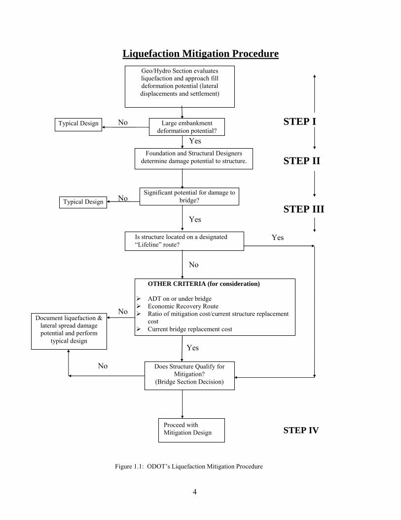
The policy further specifies that, “All bridges should be evaluated for liquefaction and lateral spread potential and the possible effects of these conditions on the structure.” Consideration is given to the magnitude of the anticipated lateral soil deformation, the influence of piles on embankment deformations, and tolerable deformation limits of the structures under consideration. Close coordination between the geotechnical engineer and the bridge design engineer is required. A flow chart for the mitigation procedure is provided in Figure 1.1.

A key element for implementing the ODOT liquefaction mitigation procedure is the estimation of seismically-induced ground deformations (with or without liquefaction hazards). Current methods for evaluating deformations of embankments include simplified design charts based on sliding-block methods of analysis, site-specific slope stability analysis combined with sliding-block analysis, and numerical modeling. The level of effort required for these techniques varies significantly, as does the uncertainty in the computed deformation. In order to optimize the resources for seismic and liquefaction hazard assessments, simplified, straightforward screening tools are needed. In Oregon, there are over 5,400 bridges greater than 6 m in length that span waterways. These bridges may require preliminary evaluations for liquefaction hazards. ODOT is charged with managing approximately 2,640 bridges, of which about 65% are over water (foundations on or in saturated soils). Of this subset, only 16% are supported on non-liquefiable, dense soil or rock; the remaining bridges are founded on potentially liquefiable deposits. It also is important to note that 44% of the bridge foundations in saturated soils are supported by piles.

There is a demonstrated need for improved predictive methods for evaluating liquefaction damage to highway structures. When considering the seismic retrofit of bridge foundations and embankments, however, it is desirable to reduce conservatism in assessing the magnitude of post-liquefaction deformations, prior to developing specifications for ground remediation. The primary purpose of this report is to provide specific guidance on the evaluation of post-liquefaction deformations and the possible effects of these deformations on bridges. This is intended not only to assist engineers with the methods of evaluating the liquefaction susceptibility of soils, but also to develop strategies for mitigating the liquefaction susceptibility of foundation soils at existing bridge sites.

3

Liquefaction Mitigation Procedure

Typical Design No STEP I Yes

Large embankment deformation potential?

Geo/Hydro Section evaluates liquefaction and approach fill deformation potential (lateral displacements and settlement)

STEP II

Typical Design No STEP III Yes

Significant potential for damage to bridge?

Foundation and Structural Designers determine damage potential to structure.

Yes Yes

No No

Document liquefaction & lateral spread damage potential and perform

typical design Yes No

Does Structure Qualify for Mitigation?

(Bridge Section Decision)

Is structure located on a designated “Lifeline” route?

OTHER CRITERIA (for consideration)

� ADT on or under bridge � Economic Recovery Route � Ratio of mitigation cost/current structure replacement

cost � Current bridge replacement cost

STEP IV

Proceed with Mitigation Design

Figure 1.1: ODOT’s Liquefaction Mitigation Procedure

4

For the construction of new bridges, extensive field and laboratory tests may not be available when the alternative sites are under review. Also, relatively small structures of routine importance may not economically justify large-scale exploration, sampling, and laboratory testing programs. In these instances, the lack of requisite geotechnical data precludes rigorous analysis of seismic performance and more simplified approaches are warranted for planning and preliminary design. A primary objective of this project was to synthesize existing analysis procedures with advanced numerical modeling to develop simple, straightforward methods of estimating earthquake deformations on embankments for design applications where resources, or the importance of the structure, do not justify the use of sophisticated numerical models. The methods discussed can be considered screening tools for identifying vulnerable sites as well as preliminary design tools. The following objectives were developed for this project.

1. Review the technical literature and establish a database of case histories. 2. Provide a synopsis of the literature to evaluate liquefaction hazards with emphasis on the

most widely adopted, standard-of-practice methods for use by ODOT engineers. 3. Evaluate the applicability of current standard-of-practice methods for deformation

analyses for embankments. 4. Perform a suite of numerical dynamic effective stress analyses for comparison against

the more routine sliding-block methods. 5. Develop recommendations for evaluating seismically-induced deformations of

embankments at sites with or without soil improvement. 1.2.2 Scope of Work

The scope of work for each of these objectives is outlined below.

1.2.2.1 Establish a Database of Case Histories

An extensive technical literature search was conducted to collect case histories on the seismic performance of bridges in liquefiable soils. The literature review was used to evaluate the performance of bridges and appurtenant structures, and to determine the controlling variables used in design. The results of this review are contained in Chapter 2 and the Appendix.

1.2.2.2 Literature Synopsis to Evaluate Liquefaction Hazards

Current methods for evaluating the liquefaction susceptibility of soils are based on field performance and laboratory testing of clean sand and silty sand. Recent workshops have addressed the strengths and limitations of these evaluation procedures as they apply to predominantly sandy soils. However, key issues remain unresolved. One issue is the dynamic behavior of predominantly silty soil. Silts are common in many regions of Oregon (along the Columbia and Willamette Rivers, Portland West Hills and adjoining regions, coastal regions of the state) and there was little data for characterizing the liquefaction resistance, or the post-liquefaction behavior of silty soils. For this objective, data was collected from the technical literature and laboratory research conducted on regional silts. The results of several extensive investigations on silty soils from the

5

Pacific Northwest also are summarized. The influence of pertinent factors such as gradation of the fine-grained components, soil plasticity, and stress history are addressed.

1.2.2.3 Evaluation of Current Methods of Deformation Analyses

An extensive literature search also was conducted to determine the current standard-of-practice design methods, and the applicability of these methods against the failure modes identified from the case histories. The search resulted in the collection of the traditional methods used in the seismic design of embankments and natural slopes, and recent additions that account for limitations of the standard-of-practice design methods.

1.2.2.4 Perform Numerical Dynamic Modeling Studies

Numerical modeling studies were performed to model the behavior of embankments underlain by liquefiable soils and treated soils. This objective utilized the geomechanical-modeling program FLAC 3.4 (Itasca Consulting Group 1997). The FLAC model was used to perform parametric studies of the seismic performance of embankments subjected to a suite of different earthquake ground motions. The parametric studies were used to determine the influence of several design and remediation factors on computed deformations. These included:

� static factor of safety of the embankment; � thickness of the liquefiable layer; � embankment geometry; � depth to the groundwater table; � extent of ground treatment by soil densification; and � ground motion characteristics.

1.2.2.5 Development of Design Recommendations and Basic Guidelines

The results of the numerical analyses were used to develop an improved seismic design procedure that incorporates all of the parametric study data, and includes data incorporated from the literature review. Design recommendations also were developed that highlight the usage of a simple design chart and more importantly, the assumptions and limitations of using the chart for design purposes.

1.2.3 Report Organization

This report is organized into the following five inter-related subsections.

1. An introduction to liquefaction-related damage to bridges, bridge foundations and approach embankments during historic earthquakes (Chapter 2 and Appendix).

2. An overview of methods for evaluating the liquefaction susceptibility of sandy and silty soils, as well as the post-cyclic loading behavior of these soils (Chapters 3 and 4).

3. A cursory overview of ground treatment techniques for mitigating liquefaction hazards at bridge sites (Chapter 5).

6

4. Numerical modeling and parametric studies of the seismic performance of bridge approach embankments for sites with and without soil improvement (Chapters 6 and 7).

5. A comprehensive design example for a site located in the Portland metropolitan area (Chapter 8).

Chapter 2 highlights the liquefaction-induced damage modes that have been observed at bridge sites during significant earthquakes over the past four decades. It is supplemented with a catalog of case histories that details specific aspects of the bridge damage including pertinent seismologic data (if available) and an overall damage rating (see Appendix).

Chapter 3 provides a synopsis of the standard-of-practice methods for evaluating the liquefaction susceptibility of sandy and silty soils. Guidelines outlined in the technical literature for sandy soils are augmented with region specific data for the liquefaction resistance and post-liquefaction behavior of silts. Chapter 4 details the current procedures for assessing liquefaction-induced ground deformations. This includes empirical methods of estimating lateral spread displacements due to liquefaction and methods for estimating the shear strength of liquefied soils for use in standard limit equilibrium slope stability analyses.

Chapter 5 addresses ground treatment strategies for mitigating liquefaction hazards. This chapter provides an overview of the methods employed for mitigating liquefaction hazards and provides a list of pertinent references for more in-depth reading. Chapter 6 introduces the numerical dynamic effective stress model that was employed in this project. The constitutive soil model and excess pore pressure generation scheme is outlined, along with the strengths and limitations of the model.

Chapter 7 presents a comparison of existing methods for estimating seismic deformations of embankments, the results of the numerical parametric study, and recommendations for displacement-based design procedures. It suggests a refinement to the empirical lateral displacement estimation procedures presented in Chapter 4. This is accomplished by utilizing numerical modeling tools to develop a practice-oriented design procedure that can be readily used. In these charts, a pseudo-static slope stability factor of safety is first used to predict the behavior of an embankment overlying liquefiable materials. This factor of safety is then related, via numerical modeling techniques, to the amount of embankment deformation that may be expected. Finally, recommendations are provided for estimating the volume of improved soil required to mitigate the liquefaction hazard and reduce embankment deformations.

The culmination of this investigation is contained in Chapter 8, which provides a comprehensive design application for a project site along the Columbia River in the Portland metropolitan area. The site was selected because of the considerable geotechnical data collected at the site, the existence of both sandy and silty foundation soils, the relative importance of several seismic source zones, its proximity to two major bridges and a major highway, and plans for the construction of new bridges in the area. The analysis includes a multi-hazard assessment, comprehensive liquefaction evaluation, deformation estimates obtained by several different methods, and an evaluation of the effectiveness of soil improvement for minimizing earthquake-induced deformations. Chapter 9 provides a summary and the conclusions of this project and recommendations for future work.

7

2.0 OVERVIEW OF LIQUEFACTION-INDUCED DAMAGE TO BRIDGE APPROACH EMBANKMENTS

AND FOUNDATIONS

2.1 INTRODUCTION

The reconnaissance reports of several recent earthquakes document numerous cases of significant damage to bridge foundations and abutments from liquefaction-induced ground failures. Additional documentation on the damage to highways, bridges, and embankments from liquefaction of loose, saturated, cohesionless soils clearly points out the need to develop improved criteria to identify the damage potential of both new and existing highway structures.

Lateral ground deformations due to cyclic loading have been a major source of bridge failures during historic earthquakes. Most damage of this type occurs at river crossings where bridges are founded on thick, liquefiable deposits of floodplain alluvium. Bridge piers and abutments are usually transported riverward with the spreading ground. Associated differential displacements between foundation elements generate large shear forces in connections and compressional forces in the superstructure. These forces have sheared connections, allowing decks to be thrust into, through, or over abutment walls or causing decks to buckle. In other instances, connections have remained intact with the deck acting as a strut, holding tops of piers and abutments in place while the bases of these elements are displaced toward the river (Youd 1993).

In the past four decades, there have been numerous reports on damage to bridge foundations as a result of liquefaction. For example, liquefaction-induced ground deformations were particularly destructive to highway and railway bridges during the 1964 Alaska Earthquake (Bartlett and Youd 1992). Ninety-two highway bridges were severely damaged or destroyed and an additional 49 received moderate to light damage. Approximately $80 million in damage (1964 value) was incurred by 266 bridges and numerous sections of embankment along the Alaska Railroad and Highway (Kachadoorian 1968; McCulloch and Bonilla 1970). More recently, numerous bridge failures occurred during the 1995 Hyogo-Ken Nanbu (Kobe) Earthquake (Shinozuka 1995; Matsui and Oda 1996; Tokimatsu et al. 1998). The Harbor Highway, a newer route with modern bridge structures located adjacent to Osaka Bay, suffered major damage as a result of severe liquefaction and large soil movements. Every bridge on the Harbor Highway from Nishinomiya to Rokko Island suffered damage and the highway was subsequently closed. Liquefaction-induced ground deformations have caused similar damage in many recent earthquakes in Costa Rica, Japan, and the Philippines. These reports clearly demonstrate the hazard associated with the liquefaction of soils, and provide valuable case histories on the behavior of soils as well as the structural response and modes of failure associated with damage to bridges.

The modes of damage observed during past earthquakes reflect numerous site-specific factors. In addition to the seismic and geologic hazards, bridge design and construction has a significant influence on the seismic performance. The ODOT bridge inventory includes over 2,600 bridges

9

of various size and type, design and construction, construction materials, foundation configuration, historic significance, and importance as lifelines. As outlined in the Liquefaction Mitigation Policy (ODOT 1996), some level of seismic hazard evaluation is required in order to prioritize remedial construction. Because of the resources needed for a system-wide assessment of seismic hazards, the initial prioritization will likely involve classifying bridges in terms of their importance. Those deemed essential lifelines will require further evaluation. In order to assist ODOT engineers in identifying potential seismic damage modes, this chapter provides a broad overview of liquefaction-induced ground deformations and the associated damage to bridge foundations for several previous earthquakes.

The prediction of potential ground failure modes and associated structural damage will provide the design engineer with information on which to base remedial design recommendations. Generally, two pieces of information are required to determine bridge safety against ground failure: (1) an estimate of seismic ground displacement, and (2) an assessment of the seismic performance of the bridge components subjected to the ground displacements.

2.2 LIQUEFACTION-INDUCED BRIDGE DAMAGE

Lateral soil deformations (lateral spreading) have proven to be the most pervasive type of liquefaction-induced ground failure (Youd 1993). Lateral spreading involves the movement of relatively intact soil blocks on a layer of liquefied soil toward a free face or incised channel. These blocks are transported down-slope or in the direction of a channel by both dynamic and gravitational forces. The amount of lateral displacement typically ranges from a few centimeters to several meters and can cause significant damage to engineered structures.

Experience gained from numerous earthquakes demonstrates that liquefaction-induced ground failures have been a major cause of damage to bridges built across streams and rivers. In the United States, this became apparent as early as 1906 when lateral spreads generated during San Francisco Earthquake damaged bridge structures throughout the central and northwest coastal regions of California. A county bridge over the Pajaro River demonstrated the damaging affects of large lateral displacement of the floodplain on the pile foundation and abutment (Youd 1993). The abutment displaced and was subsequently fractured due to lateral spreading of the surrounding soils toward the river (Figure 2.1). The deck, which remained attached to the tops of the piers, acted as a strut, holding the tops of the piers in place while their bases shifted riverward. This behavior demonstrated that if the superstructure is sufficiently strong, it can act as a strut, bracing the tops of abutments and piers and holding them relatively in place while the bases of these elements shift streamward with the spreading ground.

A more recent example of ground deformation is provided by the 1991 Costa Rica Earthquake, where severe damage was sustained by roads, bridges, railways and ports (Shea 1991). The roadway approach to the bridge over the Rio Estrella River experienced lateral displacements as large as 1 to 3 meters. The depths of grabens that formed due to the loss of bearing strength and lateral spreading exceeded 2 to 3 meters.

Although bridge failures are most commonly associated with lateral spreading, it is not the only potentially damaging failure mechanism. Subsidence and increased lateral pressures can also have severe consequences. During the Kobe Earthquake, Port Island settled an average of

10

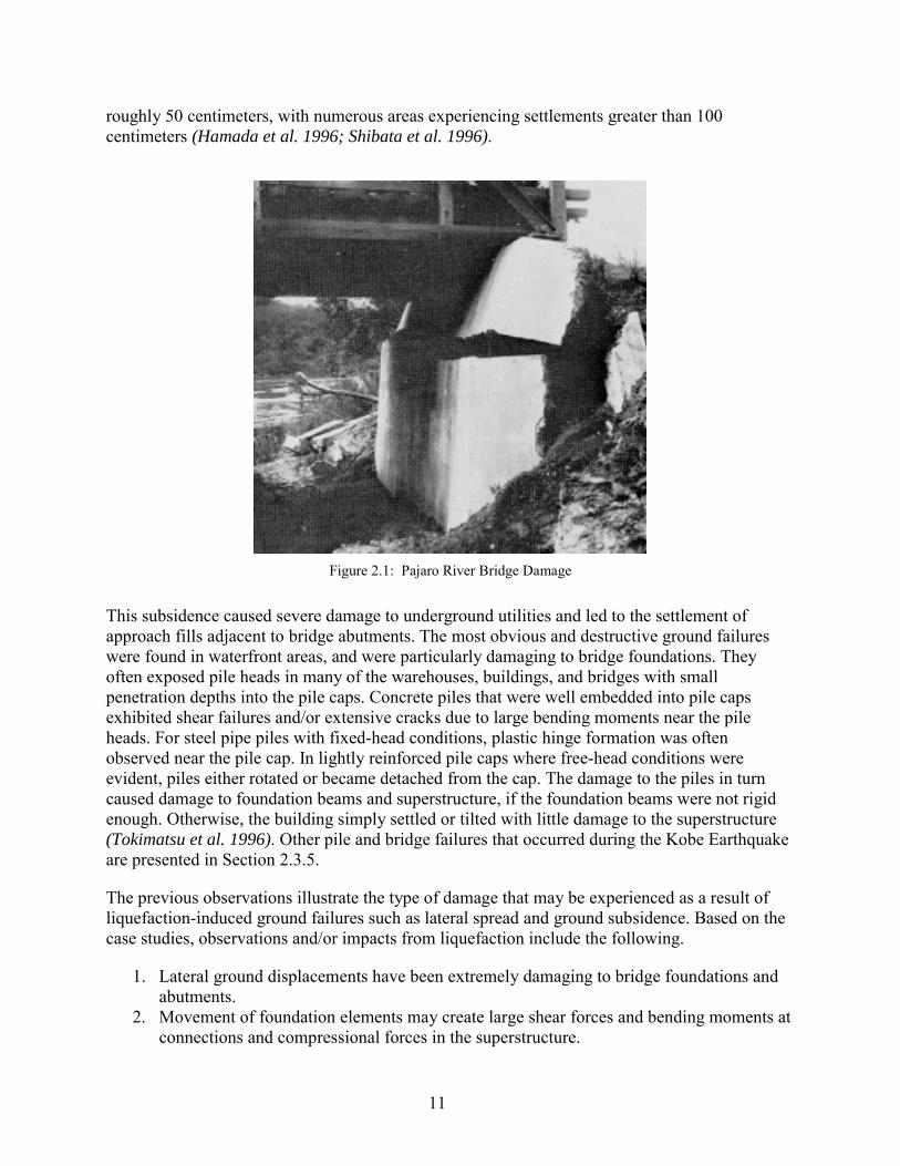
roughly 50 centimeters, with numerous areas experiencing settlements greater than 100 centimeters (Hamada et al. 1996; Shibata et al. 1996).

Figure 2.1: Pajaro River Bridge Damage

This subsidence caused severe damage to underground utilities and led to the settlement of approach fills adjacent to bridge abutments. The most obvious and destructive ground failures were found in waterfront areas, and were particularly damaging to bridge foundations. They often exposed pile heads in many of the warehouses, buildings, and bridges with small penetration depths into the pile caps. Concrete piles that were well embedded into pile caps exhibited shear failures and/or extensive cracks due to large bending moments near the pile heads. For steel pipe piles with fixed-head conditions, plastic hinge formation was often observed near the pile cap. In lightly reinforced pile caps where free-head conditions were evident, piles either rotated or became detached from the cap. The damage to the piles in turn caused damage to foundation beams and superstructure, if the foundation beams were not rigid enough. Otherwise, the building simply settled or tilted with little damage to the superstructure (Tokimatsu et al. 1996). Other pile and bridge failures that occurred during the Kobe Earthquake are presented in Section 2.3.5.

The previous observations illustrate the type of damage that may be experienced as a result of liquefaction-induced ground failures such as lateral spread and ground subsidence. Based on the case studies, observations and/or impacts from liquefaction include the following.

1. Lateral ground displacements have been extremely damaging to bridge foundations and abutments.

2. Movement of foundation elements may create large shear forces and bending moments at connections and compressional forces in the superstructure.

11

3. Compressional forces generated by lateral ground displacement generally cause one of the following reactions: (a) the superstructure may act as a strut, bracing the tops of abutments and piers and holding them relatively in place while the bases of these elements shift streamward with the spreading ground; (b) the connections between the foundation and the superstructure may fail, allowing piers and abutments to shift or tilt toward the river with little restraint; or (c) the deck may buckle laterally or vertically, causing severe damage to the superstructure.

4. Subsidence and increased lateral earth pressures can also lead to deleterious consequences for bridge foundations. Waterfront retaining structures, especially in areas of reclaimed land, can experience large settlements and lateral earth pressures adjacent to bridge foundations. These movements lead to the rotation and translation of bridge abutments and increased lateral forces on pile foundations.

5. A number of failure modes may occur in pile foundations, depending on the conditions of fixity, pile reinforcement and ductility. Generally, if concrete piles were well embedded in the pile caps, shear or flexural cracks occurred at pile heads, often leading to failure; if steel pipe piles were fixed tightly in the pile caps, failure was at the connection or pile cap; or if the pile heads were loosely connected to the pile caps, they either rotated or were detached.

To better understand these phenomena and the potential ramifications, several case histories are examined in greater detail in the subsequent section.

2.3 OVERVIEW OF HISTORIC DAMAGE TO BRIDGE FOUNDATIONS

The modes and extent of seismic damage to bridges can be related to the movement of abutments, lateral spreading and settlement of abutment fills, horizontal displacement and tilting of piers, severe differential settlement of abutments and piers, and failure of foundation members. The ability to predict ground failures and associated structural damage are requisites for seismic resistant design and evaluation of existing structures.

2.3.1 1964 Alaska Earthquake

The Great Alaska Earthquake of 1964 (Mw 9.2) caused some of the most devastating and widespread damage to highway bridges in United States history. The peak ground accelerations were estimated to be in the 0.10 g to 0.20 g range. Although these values seem quite small considering the amount of damage, the duration and frequency of the ground motions are equally important in describing the damage potential of an earthquake. The duration of strong shaking was estimated to be anywhere between 1.5 to 3.0 minutes, and because of the large epicentral distances to many bridges, the ground motions were likely robust at longer periods (closer to fundamental periods of the structures). The seismic performance of the transportation system in Alaska during this event is particularly germane for Oregon because of the potential for large subduction zone earthquakes in the Pacific Northwest (this seismic hazard is addressed in Chapter 8).

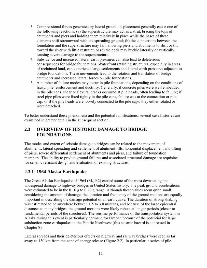
Lateral spreads and their deleterious effects on highway and railway bridges were seen as far away as 130 km from the zone of energy release (Figure 2.2). In particular, a series of pile-

12

supported bridges along the Seward and Copper River Highways suffered extensive damage (Ross et al. 1973). Thorough summaries of the damage sustained to Alaska highways have been presented by Bartlett and Youd (1992), and Ross and others (1973). In most instances, the damage could be attributed to liquefaction of abutment fills and/or foundation soils.

Figure 2.2: Area of Damage of 1964 Alaska Earthquake

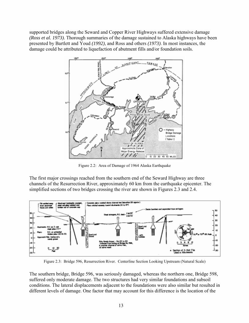
The first major crossings reached from the southern end of the Seward Highway are three channels of the Resurrection River, approximately 60 km from the earthquake epicenter. The simplified sections of two bridges crossing the river are shown in Figures 2.3 and 2.4.

Figure 2.3: Bridge 596, Resurrection River. Centerline Section Looking Upstream (Natural Scale)

The southern bridge, Bridge 596, was seriously damaged, whereas the northern one, Bridge 598, suffered only moderate damage. The two structures had very similar foundations and subsoil conditions. The lateral displacements adjacent to the foundations were also similar but resulted in different levels of damage. One factor that may account for this difference is the location of the

13

piers in relation to the channel margins. In Bridge 596, the abutment fills extended almost to the piers so that horizontal displacement of the fills exerted high lateral loads on the pier footings and piers, causing rotation and cracking of the pier wall as shown in Figure 2.5.

Figure 2.4: Bridge 598, Resurrection River. Centerline Section Looking Upstream (Natural Scale)

In Bridge 598, a clearance of 6 m between the toes of the abutments and the piers provided space for displaced soil to accumulate and reduced the likelihood of high lateral loading of the pier foundations. The location of abutments is significant. Standard penetration tests (SPT) at this location gave blow counts of N = 30 to 60 blows/ft for the silty, sandy gravel in the area. Such values would not be considered conducive to liquefaction failures of a 6-m high embankment with 1.5:1 slopes. However, limited tests were performed and blow counts are not a good indication of the relative density of sands in gravelly material, mainly due to the small inside diameter of the split-spoon sampler used during testing. High pore pressure buildup in the sand lenses or partial liquefaction most likely contributed to lateral spreading of the abutment fill.

Figure 2.5: Bridge 596

14

Another area of extensive bridge damage was where the Seward Highway crossed the valley of the Snow River, where it forms a delta into the southern end of Kenai Lake. Four bridges were in service at the time of the earthquake, all were founded on timber bents and all were damaged to differing extents. Bridge 605 was located approximately midway across the valley. At the time of the earthquake, a replacement bridge (Bridge 605A) was under construction immediately adjacent on the downstream side. Bridge 605 was completely destroyed as shown in the centerline section of Figure 2.6 and the post-earthquake view in Figure 2.7.

Figure 2.6: Bridge 605, Snow River 3. Centerline Section Looking Downstream (Natural Scale)

Figure 2.7: Bridge 605, Snow River 3. Post-earthquake View, Looking Downstream.

15

Liquefaction-induced movements of the abutment fills and foundation soils caused the abutments to move toward one another, compressing and buckling the superstructure. Many of the timber bents settled, or were driven, nearly 3 m downward. The timber piling extended about 12 m to 18 m into the fluvial soil (mainly sand and silts) with SPT blow counts of N = 5 to 10 blows/ft. Some pile tips may have extended into material of N ≈ 30 blows/ft. Bridge 605A was under construction and experienced significant displacement and tilting as shown in Figure 2.8. The pier foundations were founded on concrete-fill steel-tube piles extending to an average depth of 27 m below the level of the streambed. As a result of liquefaction, these piers displaced laterally about 2.5 m downstream and tilted upstream about 15� as illustrated in Figure 2.9. Eyewitness accounts confirm that liquefaction of cohesionless soils did occur in the region. Reports mentioned the occurrence of sand (mud) boils and that a 3-m high road embankment was reduced to the level of the floodplain.

Figure 2.8: Bridge 605A, Snow River 3. During Construction. Looking East from Midspan

Figure 2.9: Bridge 605A. Lateral Elevation of Pier 6 as Constructed at Time of Earthquake.

16

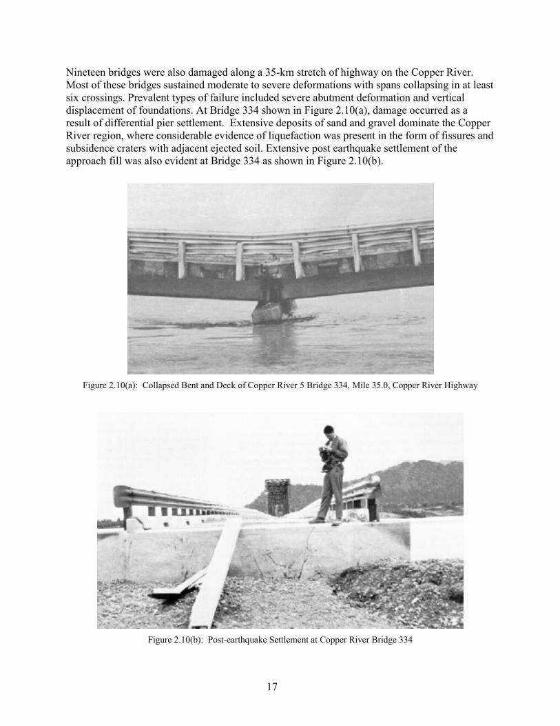
Nineteen bridges were also damaged along a 35-km stretch of highway on the Copper River. Most of these bridges sustained moderate to severe deformations with spans collapsing in at least six crossings. Prevalent types of failure included severe abutment deformation and vertical displacement of foundations. At Bridge 334 shown in Figure 2.10(a), damage occurred as a result of differential pier settlement. Extensive deposits of sand and gravel dominate the Copper River region, where considerable evidence of liquefaction was present in the form of fissures and subsidence craters with adjacent ejected soil. Extensive post earthquake settlement of the approach fill was also evident at Bridge 334 as shown in Figure 2.10(b).

Figure 2.10(a): Collapsed Bent and Deck of Copper River 5 Bridge 334, Mile 35.0, Copper River Highway

Figure 2.10(b): Post-earthquake Settlement at Copper River Bridge 334

17

The Alaska earthquake provides extensive case studies on the modes of bridge failure resulting from liquefaction. The greatest damage occurred in regions characterized by thick deposits of saturated cohesionless soils; field evidence indicates that liquefaction probably played a major role in the development of foundation displacements and bridge damage. A correlation between foundation displacement and foundation support conditions is provided in Figure 2.11, and reflects the influence of liquefaction on observed damage. The most prevalent damage was shortening of the overall span between abutments. This was associated with settlement of abutment fills. In many cases, the superstructure of the bridge had ridden over both abutments.

� � �

�

�

FOUNDATION DISPLACEMENTS

Severe Moderate Minor Nil

Founded directly on bedrock

� � � � �

Piling to bedrock through cohesionless soils

Founded on bedrock of one end of bridge, directly or via piles; embedded in cohesionless soils over remaining length

� �

Piling embedded in gravels and gravelly sands

� � � � � �

� � � � � �

�

�

Piling embedded in saturated medium to dense sand and silts (20<N<40 approx)

� � �

Piling driven into medium to dense sand silts (N>20) through saturated loose to medium-dense sands and silts (N<20)

� � � � � � � �

FOU

ND

AT

ION

SU

PPO

RT

C

ON

DIT

ION

S

Piling embedded in saturated loose to medium-dense sands and silts (N<20)

� � � � � � � � � �

� � �

Figure 2.11: Correlation between Foundation Displacements Sustained and Foundation SupBridges on the Seward, Sterling and Copper River Highways

(Data was available from only 60 of the approximately 120 bridges on the three hig

The following conclusions regarding this earthquake, as presented by Ross and summarized below.

18

�

�

� �

�

� � � �

port Conditions at

hways.)

others (1973), are

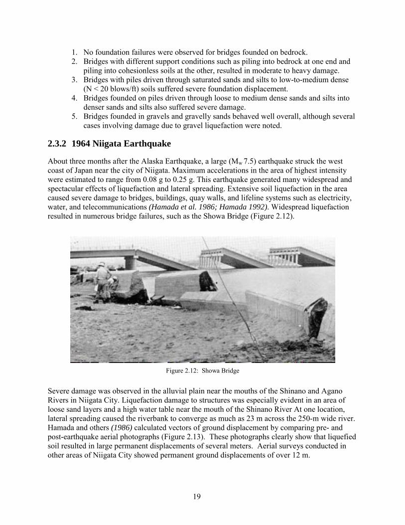
1. No foundation failures were observed for bridges founded on bedrock. 2. Bridges with different support conditions such as piling into bedrock at one end and

piling into cohesionless soils at the other, resulted in moderate to heavy damage. 3. Bridges with piles driven through saturated sands and silts to low-to-medium dense

(N < 20 blows/ft) soils suffered severe foundation displacement. 4. Bridges founded on piles driven through loose to medium dense sands and silts into

denser sands and silts also suffered severe damage. 5. Bridges founded in gravels and gravelly sands behaved well overall, although several

cases involving damage due to gravel liquefaction were noted.

2.3.2 1964 Niigata Earthquake

About three months after the Alaska Earthquake, a large (Mw 7.5) earthquake struck the west coast of Japan near the city of Niigata. Maximum accelerations in the area of highest intensity were estimated to range from 0.08 g to 0.25 g. This earthquake generated many widespread and spectacular effects of liquefaction and lateral spreading. Extensive soil liquefaction in the area caused severe damage to bridges, buildings, quay walls, and lifeline systems such as electricity, water, and telecommunications (Hamada et al. 1986; Hamada 1992). Widespread liquefaction resulted in numerous bridge failures, such as the Showa Bridge (Figure 2.12).

Figure 2.12: Showa Bridge

Severe damage was observed in the alluvial plain near the mouths of the Shinano and Agano Rivers in Niigata City. Liquefaction damage to structures was especially evident in an area of loose sand layers and a high water table near the mouth of the Shinano River At one location, lateral spreading caused the riverbank to converge as much as 23 m across the 250-m wide river. Hamada and others (1986) calculated vectors of ground displacement by comparing pre- and post-earthquake aerial photographs (Figure 2.13). These photographs clearly show that liquefied soil resulted in large permanent displacements of several meters. Aerial surveys conducted in other areas of Niigata City showed permanent ground displacements of over 12 m.

19

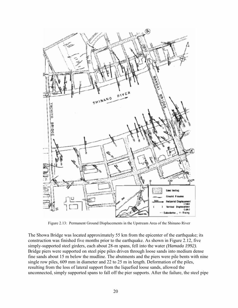
Figure 2.13: Permanent Ground Displacements in the Upstream Area of the Shinano River

The Showa Bridge was located approximately 55 km from the epicenter of the earthquake; its construction was finished five months prior to the earthquake. As shown in Figure 2.12, five simply-supported steel girders, each about 28-m spans, fell into the water (Hamada 1992). Bridge piers were supported on steel pipe piles driven through loose sands into medium dense fine sands about 15 m below the mudline. The abutments and the piers were pile bents with nine single row piles, 609 mm in diameter and 22 to 25 m in length. Deformation of the piles, resulting from the loss of lateral support from the liquefied loose sands, allowed the unconnected, simply supported spans to fall off the pier supports. After the failure, the steel pipe

20

piles supporting the fourth pier, located within the river, were extracted and examined. Their deformed shapes indicate that about 0.5 m of lateral displacement occurred at the level of the riverbed and that ground displacement reached depths as great as 7 to 8 m below the bed. The left abutment moved about 1 m toward the center of the river, and its approach road settled considerably. Hamada (1992) noted that horizontal displacement of the piers supporting the Showa Bridge was much less than the displacement of the ground a short distance either upstream or downstream from the bridge. This reduced displacement indicates that the bridge restrained ground deformation.

Further evidence of the influence of pile foundations on lateral spread displacement is illustrated by the aerial photographs of Hamada (1992). Calculated vectors of ground displacement indicate that riverbank displacements were about 8 to 9 m upstream from the Bandai Bridge in Niigata City, and only about 4 to 5 m near the bridge. Therefore, the bridge apparently restrained lateral ground movement by about 4 m.

Immediately downstream of the Showa Bridge is the Yachiyo Bridge. Its pier foundations were pushed toward the river due to large ground displacements while displacement at the top of the piers was restrained because of the resistance of the girders. The damage to the abutments and piers is shown in Figures 2.14 and 2.15. The foundations of the abutments and piers P1 and P2 had been constructed on reinforced concrete piles with a diameter of 300 mm and a length of about 10 m. Pier 2 was broken at the level of the ground surface with the permanent deformation between the top of the broken pier and the lower part of the pier being 1.1 m. It was reported that the pile was severely damaged about 8 m from the top, and horizontal cracks, which could have been caused by large bending moments, were found throughout both piles.

Figure 2.14: Damage to Yachiyo Bridge 5, 6

This earthquake also provided Hamada (1992) an opportunity to make detailed measurements of reinforced concrete pile deformations caused by lateral spreads at the NHK and Niigata Family Courthouse (NFCH) Buildings. The NHK building was a four-story reinforced concrete building supported on reinforced concrete piles 35 cm in diameter. Excavations performed 20 years after the earthquake revealed extensive damage (Figure 2.16). The NFCH was a three-story reinforced

21

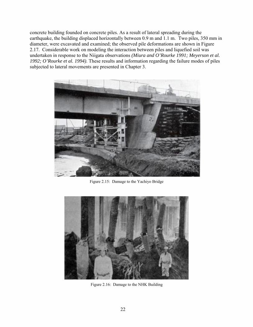
concrete building founded on concrete piles. As a result of lateral spreading during the earthquake, the building displaced horizontally between 0.9 m and 1.1 m. Two piles, 350 mm in diameter, were excavated and examined; the observed pile deformations are shown in Figure 2.17. Considerable work on modeling the interaction between piles and liquefied soil was undertaken in response to the Niigata observations (Miura and O’Rourke 1991; Meyerson et al. 1992; O’Rourke et al. 1994). These results and information regarding the failure modes of piles subjected to lateral movements are presented in Chapter 3.

Figure 2.15: Damage to the Yachiyo Bridge

Figure 2.16: Damage to the NHK Building

22

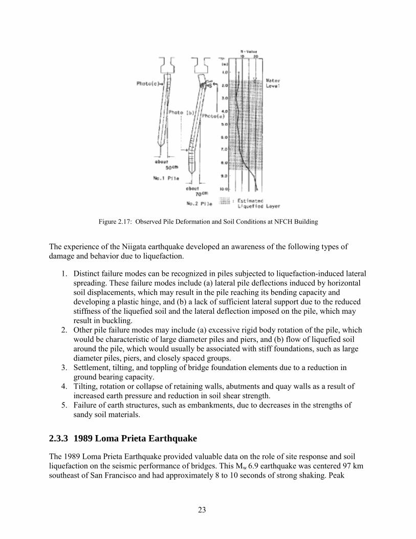
Figure 2.17: Observed Pile Deformation and Soil Conditions at NFCH Building

The experience of the Niigata earthquake developed an awareness of the following types of damage and behavior due to liquefaction.

1. Distinct failure modes can be recognized in piles subjected to liquefaction-induced lateral spreading. These failure modes include (a) lateral pile deflections induced by horizontal soil displacements, which may result in the pile reaching its bending capacity and developing a plastic hinge, and (b) a lack of sufficient lateral support due to the reduced stiffness of the liquefied soil and the lateral deflection imposed on the pile, which may result in buckling.

2. Other pile failure modes may include (a) excessive rigid body rotation of the pile, which would be characteristic of large diameter piles and piers, and (b) flow of liquefied soil around the pile, which would usually be associated with stiff foundations, such as large diameter piles, piers, and closely spaced groups.

3. Settlement, tilting, and toppling of bridge foundation elements due to a reduction in ground bearing capacity.

4. Tilting, rotation or collapse of retaining walls, abutments and quay walls as a result of increased earth pressure and reduction in soil shear strength.

5. Failure of earth structures, such as embankments, due to decreases in the strengths of sandy soil materials.

2.3.3 1989 Loma Prieta Earthquake

The 1989 Loma Prieta Earthquake provided valuable data on the role of site response and soil liquefaction on the seismic performance of bridges. This Mw 6.9 earthquake was centered 97 km southeast of San Francisco and had approximately 8 to 10 seconds of strong shaking. Peak

23

horizontal accelerations in the epicentral region were as high as 0.64 g. In the areas where damage investigations were concentrated, the peak ground accelerations generally ranged from 0.20 g to 0.40 g. Soil liquefaction and associated ground deformations were documented at numerous locations in the San Francisco Bay area (Seed et al. 1990; O’Rourke and Pease 1992).

An interesting observation was that soil liquefaction in the Monterey and San Francisco Bay areas occurred at many of the same locations that exhibited ground failures during the 1906 earthquake. These ground failures were conspicuous in the Monterey Bay/Watsonsville region. Here, liquefaction was directly responsible for the destruction of a Marine Research Facility at Moss Landing as well as damage to other structures and facilities (Seed et al. 1990; Boulanger et al. 1998a). The Research Facility was located on a sandy peninsula between the Pacific Ocean and the old trace of the Salinas River. Fissures and sand boils were found in the immediate vicinity of the facility. As illustrated in Figure 2.18, the structure settled several meters, and lateral spread deformations of the foundation soils were roughly 2 m. Similar, yet more severe lateral spreading occurred in this area during the 1906 earthquake, as shown in Figure 2.19.

Figure 2.18: Damage to the Moss Landing Research Facility due to Settlement and Lateral Spreading

24

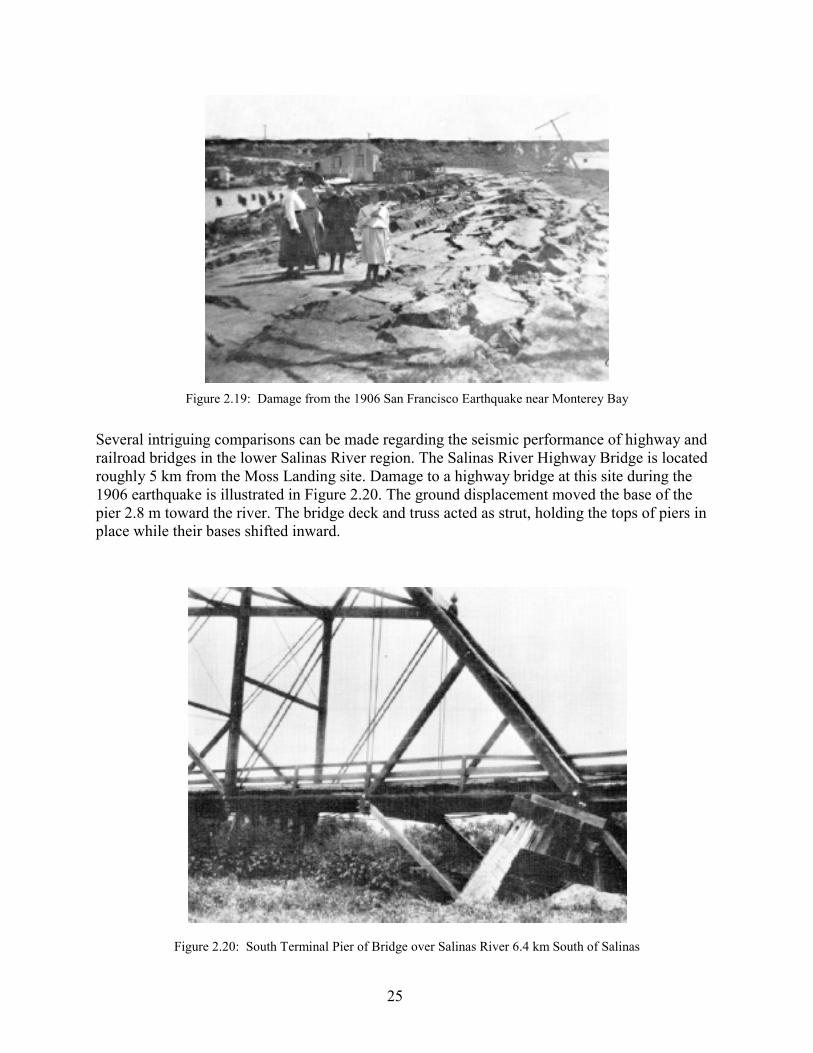
Figure 2.19: Damage from the 1906 San Francisco Earthquake near Monterey Bay

Several intriguing comparisons can be made regarding the seismic performance of highway and railroad bridges in the lower Salinas River region. The Salinas River Highway Bridge is located roughly 5 km from the Moss Landing site. Damage to a highway bridge at this site during the 1906 earthquake is illustrated in Figure 2.20. The ground displacement moved the base of the pier 2.8 m toward the river. The bridge deck and truss acted as strut, holding the tops of piers in place while their bases shifted inward.

Figure 2.20: South Terminal Pier of Bridge over Salinas River 6.4 km South of Salinas

25

In this vicinity during the 1989 earthquake, liquefaction-induced lateral spreading was once again evident as shown in Figure 2.21. The U.S. Highway 1 and adjacent frontage road bridges were undamaged by the earthquake despite evidence of sand boils, ground oscillation, and lateral spreading of approximately 0.5 meter toward the river. At this same site, relatively large lateral and vertical ground deformations were observed next to a railroad bridge as shown in Figure 2.22. However, the bridge components were not damaged during this earthquake. It is of historic interest that the bridge pier shown in Figure 2.22 was substantially damaged during the 1906 earthquake. Finally, a one-lane bridge located at Moss Landing (in close proximity to the Research Facility) sustained minor damage due to lateral spreading of the approach fill as shown in Figure 2.23.

Figure 2.21: Liquefaction-induced Lateral Spreading beneath the Salinas River Highway Bridge

26

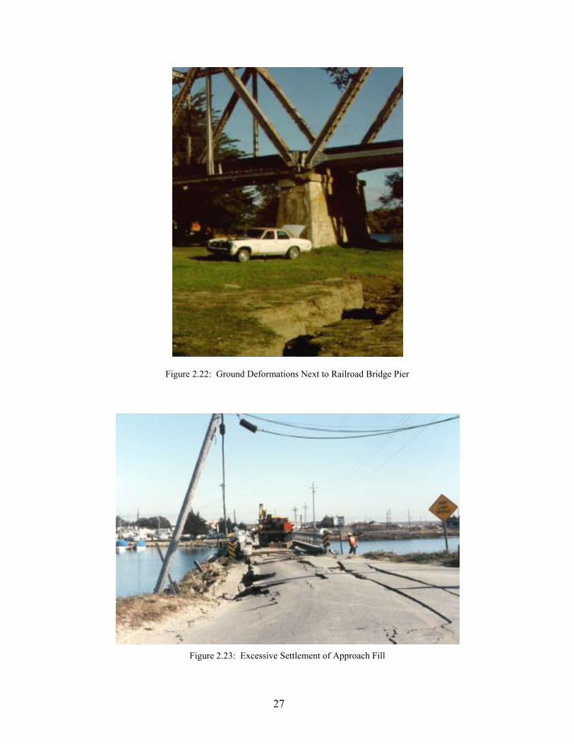
Figure 2.22: Ground Deformations Next to Railroad Bridge Pier

Figure 2.23: Excessive Settlement of Approach Fill

27

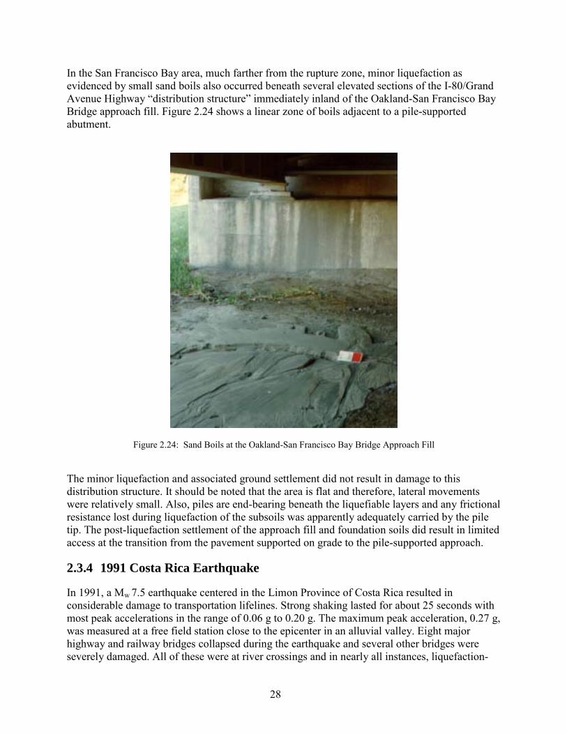
In the San Francisco Bay area, much farther from the rupture zone, minor liquefaction as evidenced by small sand boils also occurred beneath several elevated sections of the I-80/Grand Avenue Highway “distribution structure” immediately inland of the Oakland-San Francisco Bay Bridge approach fill. Figure 2.24 shows a linear zone of boils adjacent to a pile-supported abutment.

Figure 2.24: Sand Boils at the Oakland-San Francisco Bay Bridge Approach Fill

The minor liquefaction and associated ground settlement did not result in damage to this distribution structure. It should be noted that the area is flat and therefore, lateral movements were relatively small. Also, piles are end-bearing beneath the liquefiable layers and any frictional resistance lost during liquefaction of the subsoils was apparently adequately carried by the pile tip. The post-liquefaction settlement of the approach fill and foundation soils did result in limited access at the transition from the pavement supported on grade to the pile-supported approach.

2.3.4 1991 Costa Rica Earthquake

In 1991, a Mw 7.5 earthquake centered in the Limon Province of Costa Rica resulted in considerable damage to transportation lifelines. Strong shaking lasted for about 25 seconds with most peak accelerations in the range of 0.06 g to 0.20 g. The maximum peak acceleration, 0.27 g, was measured at a free field station close to the epicenter in an alluvial valley. Eight major highway and railway bridges collapsed during the earthquake and several other bridges were severely damaged. All of these were at river crossings and in nearly all instances, liquefaction-

28

induced ground displacement was the cause of damage (Shea 1991). Lateral displacement of floodplain deposits destroyed approach embankments, pushed abutments and piers riverward, and sheared connections in the substructure of the bridges.

The Rio Viscaya Bridge, a three-span pre-stressed concrete bridge founded in loose sands, collapsed due to loss of soil support and ground deformations resulting from liquefaction. The bridge lost two spans due to severe abutment rotation, resulting in pile distress (Figure 2.25) and the collapse of one interior support. A second interior support settled vertically about 1 m. Geotechnical boring logs near the north abutment showed that the entire length of piles were supported in sands and silty sands. Liquefaction of soils in approach fills caused lateral spreading and bearing capacity failure. The north roadway approach fill settled approximately 1.2 m. Both north and south abutments rotated as a result of movement of liquefied soils.

Figure 2.25: Rio Vizcaya Bridge, Pile Failures (North Abutment)

The Rio Banano Bridge provides an additional example of severe damage due to liquefaction. It was a single lane bridge consisting of three 22 m spans of twin prestressed concrete I-beams, located at a river crossing. The soil movement caused about a 9� rotation of the south abutment resulting in a movement of the pile tops toward the river of roughly 0.7 m. All piles were 36 cm square precast concrete piles. The front piles, driven at a batter of 1H:5V, suffered flexural as well as shear failures (Figure 2.26). Vertical piles at the rear portion of abutment pile caps showed less damage. As observed at other bridges, the approach fills slumped substantially and restricted access until the grade could be restored.

29

Figure 2.26: Damage due to Liquefaction at Rio Banano Bridge

2.3.5 1995 Hyogo-Ken-Nanbu (Kobe) Earthquake

The MW 6.9 Kobe earthquake was the most damaging earthquake to strike Japan since the Kanto Earthquake of 1923. Peak accelerations ranged from 0.50 g to 0.80 g near the rupture zone, and 0.20 g to 0.50 g approximately 20 km away. The duration of the strong motions was roughly 10 to 15 seconds. Widespread ground failure was observed throughout the strongly shaken region along the margin of Osaka Bay (Hamada et. al. 1995; Shibata et al. 1996). On Rokko Island and Port Island, which are reclaimed lands in Osaka Bay, liquefaction caused subsidence in inland areas of roughly 0.5 to 1.2 m. Major bridge damage resulted from the earthquake.

One of the hardest hit was the Harbor Highway located along the margins of Osaka Bay. Every bridge along this route from Nishinomiya to Rokko Island suffered damage. The entire area along the coast was subject to severe liquefaction and large soil movements. Consequently, bridge foundations that had little resistance from the weak foundation soils rocked and displaced during the earthquake. Bridge superstructures fell off their bearings, and in some cases off their substructure. There was damage at almost every expansion joint along the highway. The Rokko Island Bridge was damaged by excessive substructure movements. A bearing failure on one side of the bridge racked the arch leading to buckling the cross-framing. Other damage along the highway included the settlement of approach fills and the shattering of piers.

Bridge damage as a result of ground deformation was also experienced on the Hanshin Expressway Route 5. The Shukugawa Bridge, a three-span continuous box girder, is supported on concrete multi-column bents and pile footings (Shinosuka 1995). During the earthquake, liquefaction was widespread in the general area of the bridge and lateral spreading was evident at many locations. Both banks of the Shukugawa were subject to large soil deformations and moved towards the center of the river. Piers at either end of the bridge displaced (0.5 m to 1.0 m) with the soil and dislodged the bearings under the main girders as well as the approach spans.

30

Well-documented case histories of the seismic performance of cast-in-place bored pile foundations, raft foundations, caisson foundations, steel pipe pile foundations, and precast prestressed concrete pile foundations have demonstrated the impact of both seismic forces and forces generated by liquefaction and the lateral flow of the subsoil below the ground surface (Matsui and Oda 1996; Tokimatsu et al. 1997, 1998; Yasuda et al. 1997). The seismic performance of concrete cylinder piles, cast-in-place bored piles, and steel pipe piles with concrete in-fill has been studied extensively due to widespread use of these piles in the region. Damage inspections were made at numerous sites using a borehole television (BHTV) system, which is generally accomplished by lowering a high-resolution camera down a hole bored into a pile. The BHTV system was used to confirm that cracks were concentrated around the top of the pile where the maximum moment occurs, and at layer boundaries between soft and relative stiff soils. Matsui and Oda (1996) postulate that pile cracks may form in piles at depth due to the density of steel reinforcement changes, the location of second largest moment, and the interface between soft and hard soil layers.

Most of the long-span bridges over water were supported on gravity concrete caisson foundations. These foundations are typically constructed near waterfront retaining structures, or as integral parts of the retaining walls. The increased lateral earth pressures due to inertial effects of the strong ground motions and liquefaction of the backfill resulted in excessive deformations of caissons throughout the Kobe waterfront. In many instances, the lateral deformations of the caissons resulted in damage to bridge approach fills and pile foundations. Figure 2.27 illustrates the damage to a pile supported structure at a marine transportation facility. It is important to note that plastic hinges formed in the steel pipe piles at depth. This was due in part to a substantial variation in the stiffness and strength of the upper marine clay and sand units relative to the underlying stiff clay and dense gravel deposits. The lateral displacement of the wharf deck due to pile deformation varied from roughly 0.5 to 1.5 m at this site.

Figure 2.27: Damage to Pile Structure at Marine Facility

31

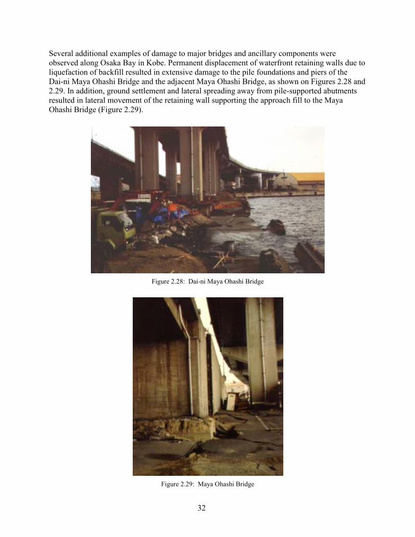
Several additional examples of damage to major bridges and ancillary components were observed along Osaka Bay in Kobe. Permanent displacement of waterfront retaining walls due to liquefaction of backfill resulted in extensive damage to the pile foundations and piers of the Dai-ni Maya Ohashi Bridge and the adjacent Maya Ohashi Bridge, as shown on Figures 2.28 and 2.29. In addition, ground settlement and lateral spreading away from pile-supported abutments resulted in lateral movement of the retaining wall supporting the approach fill to the Maya Ohashi Bridge (Figure 2.29).

Figure 2.28: Dai-ni Maya Ohashi Bridge

Figure 2.29: Maya Ohashi Bridge

32

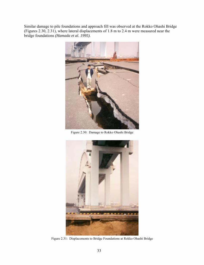
Similar damage to pile foundations and approach fill was observed at the Rokko Ohashi Bridge (Figures 2.30, 2.31), where lateral displacements of 1.8 m to 2.4 m were measured near the bridge foundations (Hamada et al. 1995).

Figure 2.30: Damage to Rokko Ohashi Bridge

Figure 2.31: Displacements to Bridge Foundations at Rokko Ohashi Bridge

33

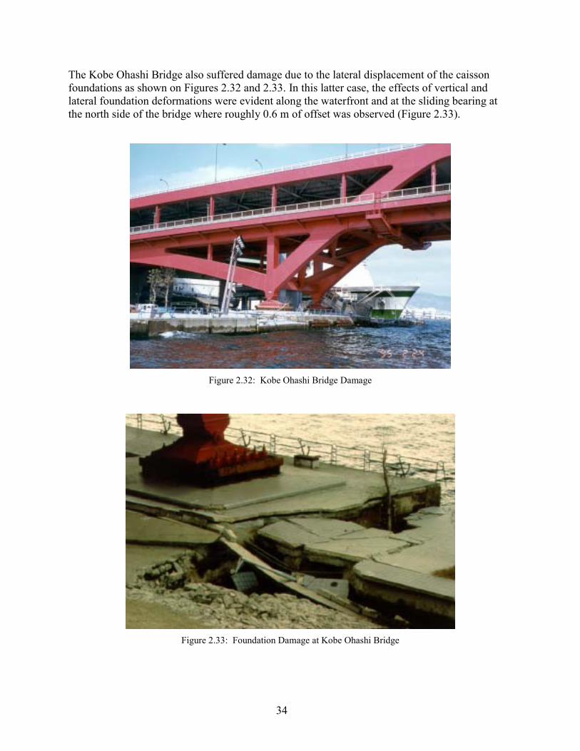
The Kobe Ohashi Bridge also suffered damage due to the lateral displacement of the caisson foundations as shown on Figures 2.32 and 2.33. In this latter case, the effects of vertical and lateral foundation deformations were evident along the waterfront and at the sliding bearing at the north side of the bridge where roughly 0.6 m of offset was observed (Figure 2.33).

Figure 2.32: Kobe Ohashi Bridge Damage

Figure 2.33: Foundation Damage at Kobe Ohashi Bridge

34

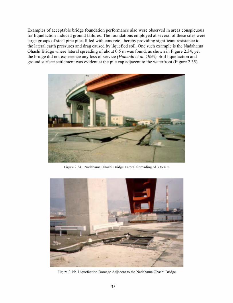
Examples of acceptable bridge foundation performance also were observed in areas conspicuous for liquefaction-induced ground failures. The foundations employed at several of these sites were large groups of steel pipe piles filled with concrete, thereby providing significant resistance to the lateral earth pressures and drag caused by liquefied soil. One such example is the Nadahama Ohashi Bridge where lateral spreading of about 0.5 m was found, as shown in Figure 2.34, yet the bridge did not experience any loss of service (Hamada et al. 1995). Soil liquefaction and ground surface settlement was evident at the pile cap adjacent to the waterfront (Figure 2.35).

Figure 2.34: Nadahama Ohashi Bridge Lateral Spreading of 3 to 4 m

Figure 2.35: Liquefaction Damage Adjacent to the Nadahama Ohashi Bridge

35

Other structures at this site supported by smaller pile groups or lightly reinforced piles, exhibited severe damage as shown in Figures 2.36 and 2.37. The Nadahama Bridge is visible in the background of Figure 2.36.

Figure 2.36: Damage to Structures near the Nadahama Ohashi Bridge

Figure 2.37: Damage to Pile Foundations near the Nadahama Ohashi Bridge

36

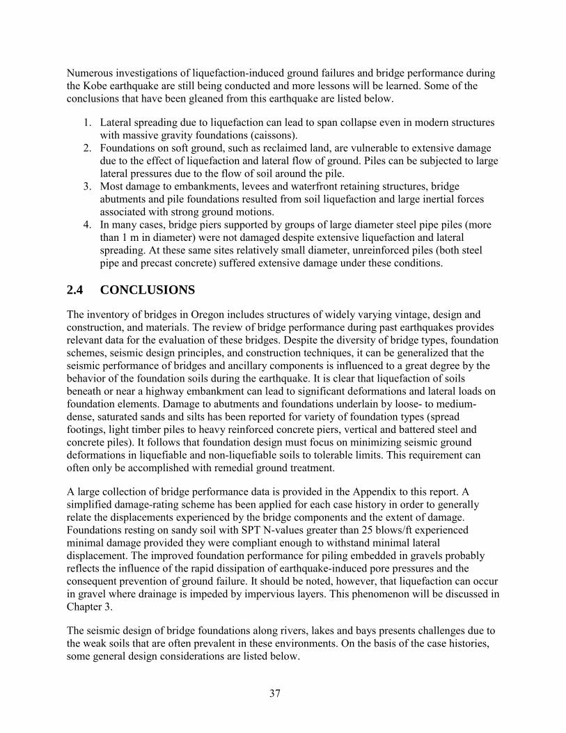
Numerous investigations of liquefaction-induced ground failures and bridge performance during the Kobe earthquake are still being conducted and more lessons will be learned. Some of the conclusions that have been gleaned from this earthquake are listed below.

1. Lateral spreading due to liquefaction can lead to span collapse even in modern structures with massive gravity foundations (caissons).

2. Foundations on soft ground, such as reclaimed land, are vulnerable to extensive damage due to the effect of liquefaction and lateral flow of ground. Piles can be subjected to large lateral pressures due to the flow of soil around the pile.

3. Most damage to embankments, levees and waterfront retaining structures, bridge abutments and pile foundations resulted from soil liquefaction and large inertial forces associated with strong ground motions.

4. In many cases, bridge piers supported by groups of large diameter steel pipe piles (more than 1 m in diameter) were not damaged despite extensive liquefaction and lateral spreading. At these same sites relatively small diameter, unreinforced piles (both steel pipe and precast concrete) suffered extensive damage under these conditions.

2.4 CONCLUSIONS

The inventory of bridges in Oregon includes structures of widely varying vintage, design and construction, and materials. The review of bridge performance during past earthquakes provides relevant data for the evaluation of these bridges. Despite the diversity of bridge types, foundation schemes, seismic design principles, and construction techniques, it can be generalized that the seismic performance of bridges and ancillary components is influenced to a great degree by the behavior of the foundation soils during the earthquake. It is clear that liquefaction of soils beneath or near a highway embankment can lead to significant deformations and lateral loads on foundation elements. Damage to abutments and foundations underlain by loose- to medium-dense, saturated sands and silts has been reported for variety of foundation types (spread footings, light timber piles to heavy reinforced concrete piers, vertical and battered steel and concrete piles). It follows that foundation design must focus on minimizing seismic ground deformations in liquefiable and non-liquefiable soils to tolerable limits. This requirement can often only be accomplished with remedial ground treatment.

A large collection of bridge performance data is provided in the Appendix to this report. A simplified damage-rating scheme has been applied for each case history in order to generally relate the displacements experienced by the bridge components and the extent of damage. Foundations resting on sandy soil with SPT N-values greater than 25 blows/ft experienced minimal damage provided they were compliant enough to withstand minimal lateral displacement. The improved foundation performance for piling embedded in gravels probably reflects the influence of the rapid dissipation of earthquake-induced pore pressures and the consequent prevention of ground failure. It should be noted, however, that liquefaction can occur in gravel where drainage is impeded by impervious layers. This phenomenon will be discussed in Chapter 3.

The seismic design of bridge foundations along rivers, lakes and bays presents challenges due to the weak soils that are often prevalent in these environments. On the basis of the case histories, some general design considerations are listed below.

37

38

1. Overall embankment and abutment stability requires careful evaluation. It may be preferable to use longer spans and anchor abutments a suitable distance from the end of approach fills.

2. If ground treatment cannot be justified for bridges of moderate importance, clearance should be provided between the abutments and piers, if possible, to minimize the effect of abutment soil displacement on pier movement.

3. Consideration should be given to differential settlement. Severe differential settlement may occur when abutments or piers are founded on dissimilar materials or when a bridge abutment, supported on a pile foundation into a firm material, undergoes relatively small settlement compared to that of the backfill material that rests directly on the ground surface.

4. Excessive settlement between pavement sections on-grade and pile-supported approach structures has resulted in the loss of access to many bridges during past earthquakes. This can be addressed with remedial soil improvement to minimize settlements of foundation soils, or contingency plans should be made for rapid response and re-grading at important bridge sites following earthquakes.

5. Piles must be designed for appropriate ductility as soil deformations will induce curvatures and bending moments in piles.

6. With respect to the seismic performance of structural components adjacent to embankments or natural slopes, the lateral earth pressure exerted on deep foundations, abutments and/or pier walls due to non-liquefied “crusts” of competent soil translating on underlying layers of liquefied deposits must be evaluated.

7. There are a number of issues that must be considered when designing a pile to resist lateral soil deformations. Previous work has shown that damage may occur in concrete piles as a result of the position at which the density reinforcement bar changes, the location of large moments at depth, and the interface zone between soft and hard soil layers. The conditions of fixity between the pile head and the pile cap are also a critical concern when designing a pile.

8. Ground treatment may be required to insure that embankment deformations are within tolerable limits. Numerous methods of soil improvement are available (see Chapter 5). However, guidelines for the application of soil improvement at bridges are still in an early stage of development. The extent of soil improvement to be employed at a site requires an iterative approach that involves widening the block of treated soil and re-evaluating the anticipated deformations. This is addressed in Chapters 7 and 8.

3.0 EVALUATION OF LIQUEFACTION SUSCEPTIBILITY: IN SITU AND LABORATORY PROCEDURES

3.1 LIQUEFACTION HAZARD EVALUATION

The liquefaction of a loose, saturated granular soil occurs when the cyclic shear stresses and strains passing through the soil deposit induce a progressive increase in excess hydrostatic pore water pressure. During an earthquake, the cyclic shear waves that propagate upward from the underlying bedrock induce the tendency for the loose sand layer to decrease in volume. If undrained conditions are assumed, an increase in pore water pressure and an equal decrease in the effective confining stress are required to keep the loose sand at constant volume.

The degree of excess pore water pressure generation is largely a function of the initial density of the sand layer, and the intensity and duration of seismic shaking. In loose to medium dense sands, pore pressures can be generated which are equal in magnitude to the confining stress. In this state, no effective or intergranular stress exists between the sand grains and a complete loss of shear strength is temporarily experienced.

The following types of phenomena can result from soil liquefaction:

� catastrophic flow failures, � lateral spreading and ground failures, � excessive settlement, � loss of bearing capacity, � increase in active lateral earth pressures behind retaining walls, and � loss of passive resistance in anchor systems.

Two phenomena commonly occur in soils when loading cyclically: liquefaction and cyclic mobility. Because both lead to a substantial rise in pore water pressures and large strains in the laboratory, they are often confused. Generally, liquefaction occurs only in specimens that are highly contractive, whereas cyclic mobility may occur in specimens from any initial state. The difference between these phenomena and the factors affecting them, as observed in the laboratory, are summarized by Castro and Poulos (1977). In an effort to clarify some of the terminology associated with liquefaction, some definitions are provided below (Seed 1979a; Youd and Perkins 1987).

Triggering of Liquefaction or Initial Liquefaction. Denotes a condition where, during the course of cyclic stress applications, the residual pore water pressure on completion of any full stress cycle becomes equal to the applied confining pressure. The development of initial liquefaction has no implications concerning the magnitude of the soil deformations. However, it defines a condition that is a useful basis for assessing various possible forms of subsequent soil behavior.

39

Initial Liquefaction with Limited Strain Potential or Cyclic Mobility. Denotes a condition in which cyclic stress applications develop a condition of initial liquefaction. Subsequent stress applications cause limited strains to develop because of the remaining resistance of the soil to deformation or because the soil dilates; the pore pressure drops and the soil stabilizes under the applied loads. However, once the cyclic stress applications stop and if they return to the zero stress condition, there will be a residual pore water pressure in the soil equal to the overburden pressure, and this will lead to an upward flow of water in the soil which could have deleterious consequences for overlying layers.

Liquefaction with Large Strain Potential. Denotes a condition where a soil will undergo continued deformation at a constant low residual stress or with no residual resistance, due to the buildup of high pore water pressures that reduce the effective confining pressure to a very low value. The pore pressure buildup may be due to either static or cyclic stress applications.

In order to be susceptible to liquefaction, the soil must be fully saturated and subjected to a sudden or rapid loading such as that of an earthquake. The resistance of a soil to liquefaction is dependent on a combination of the soil properties, environmental factors, and characteristics of the earthquake. Soil properties such as the mineralogy, gradation or grain-size distribution, and particle shapes (e.g., angularity) all affect the soil’s liquefaction resistance. The six principal environmental factors affecting a soil’s intrinsic resistance to cyclic pore pressure generation or liquefaction during seismic loading are shown below (Seed 1992).

1. Relative Density. The resistance to cyclic pore pressure generation, as well as residual undrained strength, increase with the relative density of the soil. Relative density is the most important factor governing the liquefaction resistance of a cohesionless soil.

2. Geologic Age. The time under a sustained overburden can significantly increase the liquefaction resistance of some soils over time.

3. Prior Cyclic Load History. Prior seismic excitation can increase liquefaction resistance. This effect can also, however, be erased by more recent seismic excitation causing full or nearly full liquefaction.

4. Overconsolidation. Overconsolidation and the associated increased lateral effective confining stress can increase liquefaction resistance by increasing the coefficient of lateral earth pressure (Ko), which in turn increases the overall mean effective stress (σm′).

5. Soil Fabric. The method of deposition and compaction can have a significant influence on liquefaction resistance.

6. Drainage Characteristics. The ability to rapidly dissipate excess pore pressures, which is a function of both the permeability of the soil and the drainage boundary conditions imposed by the surrounding soils, will affect the liquefaction resistance.

One additional factor with a potentially significant impact on liquefaction resistance is the effective confining stress. Resistance to cyclic pore pressure generation and/or liquefaction increases with increased effective confining stress. As a result, site conditions involving near-surface water tables or phreatic surfaces tend to represent an inherently more liquefaction-susceptible condition than those with a deeper water table.

40

The evaluation of liquefaction hazard is generally performed in several stages: (1) preliminary geological/geotechnical site evaluation, (2) quantitative evaluation of liquefaction potential and its potential consequences, and if necessary, (3) development of mitigation and foundation remediation programs. The scope of the investigation required is dependent not only on the nature and complexity of geologic site conditions, but also on the economics of a project and on the level of risk acceptable for the proposed structure or development.

3.2 PRELIMINARY SITE INVESTIGATION

A preliminary site evaluation involves establishing the topography, stratigraphy, and location of the ground water table at the project site. These geologic site evaluations must address the following questions:

1. Are potentially liquefiable soils present? 2. Are they saturated and/or may become saturated at some future date? 3. Are they of sufficient thickness and/or lateral extent as to pose potential risk of damaging

ground deformations? Sections 3.2.1 through 3.2.3 provide additional guidance regarding the questions to be addressed in the preliminary evaluation. If this evaluation can clearly demonstrate the absence of a liquefaction hazard at a project site, then it by itself may be sufficient. If some uncertainty remains, however, then a more comprehensive geotechnical study should be undertaken. The reference, “Screening Guide for Rapid Assessment of Liquefaction Hazard at Highway Bridge Sites” (Youd 1998) provides useful information for preliminary hazard evaluations. In addition, the reference, “Guidelines for Site-specific Seismic Hazard Reports for Essential and Hazardous Facilities and Major and Special-occupancy Structures in Oregon” provides recommendations for planning the site evaluation (OBGE/OBEELS 1997).

3.2.1 Potentially Liquefiable Soil Types

The quantitative liquefaction evaluation procedures in practice are based on the behavior of predominantly sandy soils. These methods have been validated with field studies over the last three decades, and a consensus has emerged regarding their application (Youd and Idriss 1997). Understanding the liquefaction behavior of silty and gravelly soils has, however, substantially lagged. Recommendations for these soils have been largely “rules of thumb” tempered by field observations made after earthquakes. For example, cohesive soils with a fines content greater than 30%, and whose fines either classify as “clays” based on the Unified Soil Classification System (USCS), or have a plasticity index (PI) of greater than 30%, are not generally considered potentially susceptible to soil liquefaction (Seed 1992; Youd and Idriss 1997).

The influence of fine-grained soil on the liquefaction resistance of predominantly sandy soils is a topic that has received considerable attention over the past decade (Ishihara 1993, 1996; Prakash and Dakoulas 1994). Laboratory testing of silts has been performed, but to a very limited scale and with varying results (Chang 1990; Law and Ling 1992; Koester 1994; Singh 1994; Prakash et al. 1998; Guo and Prakash 1999). Recent examination of fine-grained soil behavior during earthquakes and the results of laboratory tests reveal that uniformly graded loose sandy soils that contain as much as 25% to 30% non-plastic to low plasticity fines may be highly

41

liquefiable (Chang 1990). Finn and others (1994) provide a review of the design and analysis of structures in potentially liquefiable silty soils.

In addition to sandy and silty soils, some gravelly soils and even rockfills are potentially vulnerable to liquefaction. A number of well-documented field case histories (Prakash and Dakoulas 1994) confirm that gravelly soils can liquefy. In recent years, the liquefaction behavior of gravelly soils has been investigated in the laboratory. The results and implications of these tests have been summarized by Evans and Zhou (1994). Most coarse, gravelly soils are relatively free draining; if the voids are filled with finer particles, or the surrounded soils are less pervious, then drainage may be impeded and cyclic pore pressure generation or liquefaction becomes more likely. Similarly, when they are of considerable thickness and lateral extent, deposits of coarse gravelly soils may not be capable of dissipating pore pressures and may be vulnerable to potential liquefaction.

Field evidence has shown that most liquefied gravelly soils are sand-gravel composites (Harder and Seed 1986; Evans and Harder 1993). Evans and Zhou (1994) present the results of cyclic triaxial tests on soils with increasing percentages of gravel content. They conclude that sand-gravel composites show an increase in cyclic strength with increased gravel content, even though the relative density of the composite is constant. This result raises questions about the relationship between laboratory test results and actual field behavior. Currently, the best techniques available for quantitative evaluation of the liquefaction resistance of coarse gravelly soils are those described by Harder (1988), Harder and Seed (1986), and several papers contained in Prakash and Dakoulas (1994). These methods involve two primary evaluation procedures: (1) the use of very large-scale Becker Hammer penetration resistance correlations, or (2) corrections to penetration resistances obtained by the SPT. Application and support for the former method is provided by Harder (1994), and Lum and Yan (1994), where case histories are provided to examine the application of the Becker penetration test for characterizing the liquefaction potential of gravelly soils.

In assessing the potential presence of liquefiable soil types, investigations should extend to a depth below which liquefiable soils cannot be reasonably be expected to occur. Field evidence, as observed in the Kobe and Loma Prieta earthquakes, has shown that liquefaction may occur to depths of 18.5 m. Liquefaction resistance can be roughly correlated with geologic age, depositional environment, and prior seismic history. Tables 3.1 through 3.3 present examples of geologic (and topographic) bases for preliminary estimation of liquefaction susceptibility, as summarized by Youd (1991).

Generally, geologically young natural sandy formations are most susceptible to liquefaction. Such deposits can be found in offshore, coastal, or floodplain areas when deposits are formed by the soil particles settling through water and coming to rest in a very loose state. This means that the latest Holocene deposits, typically related to the natural drainage network, are most susceptible to liquefaction. Deposits older than late Pleistocene are assumed to be not susceptible to liquefaction, based on their performance during earthquakes.

42

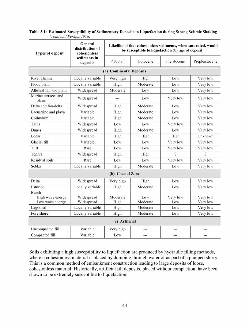
Table 3.1: Estimated Susceptibility of Sedimentary Deposits to Liquefaction during Strong Seismic Shaking (Youd and Perkins 1978)

Likelihood that cohesionless sediments, when saturated. would be susceptible to liquefaction (by age of deposit)

Types of deposit

General distribution of cohesionless sediments in

deposits <500 yr Holocene Pleistocene Prepleistocene

(a) Continental Deposits

River channel Locally variable Very high High Low Very low Flood plain Locally variable High Moderate Low Very low Alluvial fan and plain Widespread Moderate Low Low Very low Marine terraces and

plains Widespread --- Low Very low Very low

Delta and fan-delta Widespread High Moderate Low Very low Lacustrine and playa Variable High Moderate Low Very low Colluvium Variable High Moderate Low Very low Talus Widespread Low Low Very low Very low Dunes Widespread High Moderate Low Very low Loess Variable High High High Unknown Glacial till Variable Low Low Very low Very low Tuff Rare Low Low Very low Very low Tephra Widespread High High ? ? Residual soils Rare Low Low Very low Very low Sebka Locally variable High Moderate Low Very low

(b) Coastal Zone

Delta Widespread Very high High Low Very low Esturine Locally variable High Moderate Low Very low Beach

High wave energy Low wave energy

Widespread Widespread

Moderate

High

Low

Moderate

Very low

Low

Very low Very low

Lagoonal Locally variable High Moderate Low Very low Fore shore Locally variable High Moderate Low Very low

(c) Artificial

Uncompacted fill Variable Very high --- --- --- Compacted fill Variable Low --- --- ---

Soils exhibiting a high susceptibility to liquefaction are produced by hydraulic filling methods, where a cohesionless material is placed by dumping through water or as part of a pumped slurry. This is a common method of embankment construction leading to large deposits of loose, cohesionless material. Historically, artificial fill deposits, placed without compaction, have been shown to be extremely susceptible to liquefaction.

43

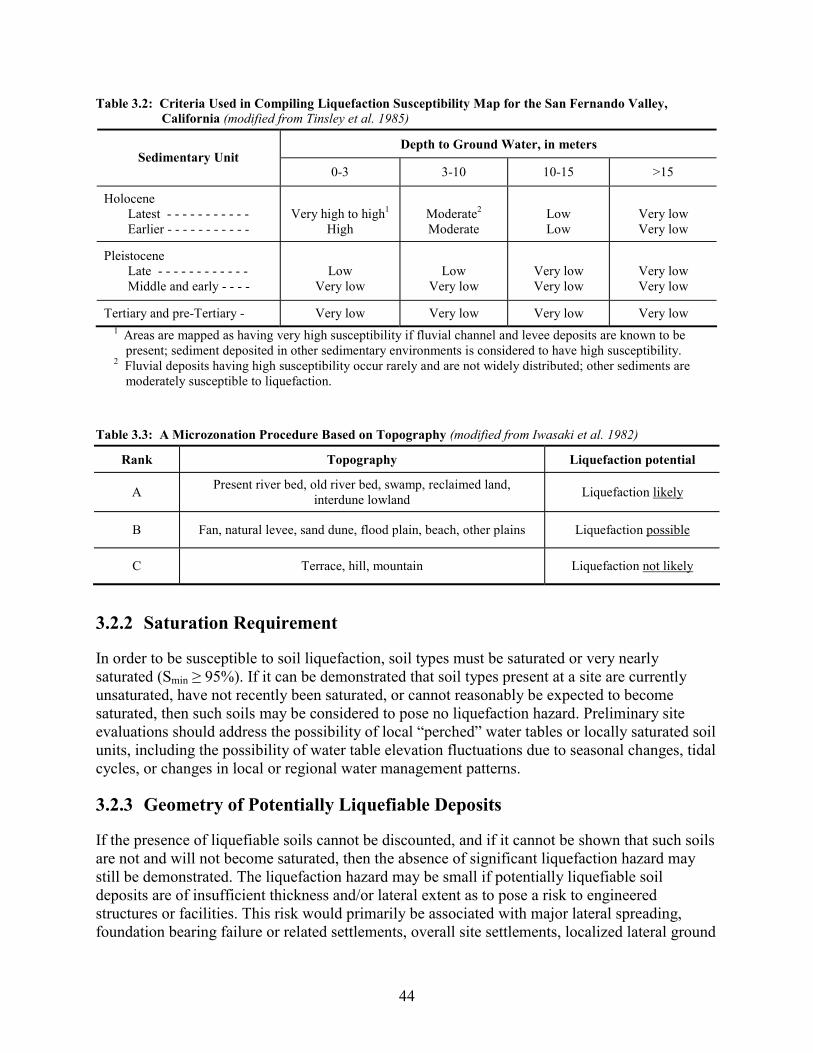
Table 3.2: Criteria Used in Compiling Liquefaction Susceptibility Map for the San Fernando Valley, California (modified from Tinsley et al. 1985)

Depth to Ground Water, in meters Sedimentary Unit

0-3 3-10 10-15 >15

Holocene Latest - - - - - - - - - - - Earlier - - - - - - - - - - -

Very high to high1

High

Moderate2

Moderate

Low Low

Very low Very low

Pleistocene Late - - - - - - - - - - - - Middle and early - - - -

Low

Very low

Low

Very low

Very low Very low

Very low Very low

Tertiary and pre-Tertiary - Very low Very low Very low Very low 1 Areas are mapped as having very high susceptibility if fluvial channel and levee deposits are known to be

present; sediment deposited in other sedimentary environments is considered to have high susceptibility. 2 Fluvial deposits having high susceptibility occur rarely and are not widely distributed; other sediments are

moderately susceptible to liquefaction.

Table 3.3: A Microzonation Procedure Based on Topography (modified from Iwasaki et al. 1982)

Rank Topography Liquefaction potential

A Present river bed, old river bed, swamp, reclaimed land, interdune lowland Liquefaction likely

B Fan, natural levee, sand dune, flood plain, beach, other plains Liquefaction possible

C Terrace, hill, mountain Liquefaction not likely

3.2.2 Saturation Requirement

In order to be susceptible to soil liquefaction, soil types must be saturated or very nearly saturated (Smin ≥ 95%). If it can be demonstrated that soil types present at a site are currently unsaturated, have not recently been saturated, or cannot reasonably be expected to become saturated, then such soils may be considered to pose no liquefaction hazard. Preliminary site evaluations should address the possibility of local “perched” water tables or locally saturated soil units, including the possibility of water table elevation fluctuations due to seasonal changes, tidal cycles, or changes in local or regional water management patterns.

3.2.3 Geometry of Potentially Liquefiable Deposits

If the presence of liquefiable soils cannot be discounted, and if it cannot be shown that such soils are not and will not become saturated, then the absence of significant liquefaction hazard may still be demonstrated. The liquefaction hazard may be small if potentially liquefiable soil deposits are of insufficient thickness and/or lateral extent as to pose a risk to engineered structures or facilities. This risk would primarily be associated with major lateral spreading, foundation bearing failure or related settlements, overall site settlements, localized lateral ground

44

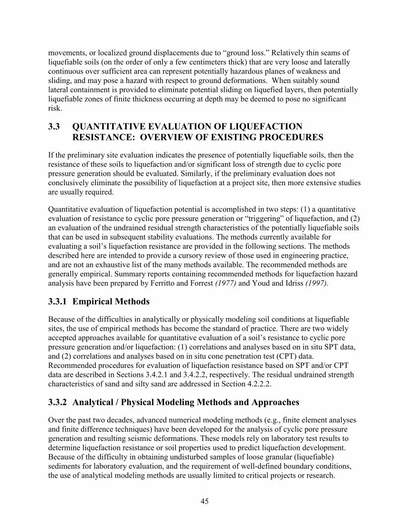
movements, or localized ground displacements due to “ground loss.” Relatively thin seams of liquefiable soils (on the order of only a few centimeters thick) that are very loose and laterally continuous over sufficient area can represent potentially hazardous planes of weakness and sliding, and may pose a hazard with respect to ground deformations. When suitably sound lateral containment is provided to eliminate potential sliding on liquefied layers, then potentially liquefiable zones of finite thickness occurring at depth may be deemed to pose no significant risk.

3.3 QUANTITATIVE EVALUATION OF LIQUEFACTION RESISTANCE: OVERVIEW OF EXISTING PROCEDURES

If the preliminary site evaluation indicates the presence of potentially liquefiable soils, then the resistance of these soils to liquefaction and/or significant loss of strength due to cyclic pore pressure generation should be evaluated. Similarly, if the preliminary evaluation does not conclusively eliminate the possibility of liquefaction at a project site, then more extensive studies are usually required.

Quantitative evaluation of liquefaction potential is accomplished in two steps: (1) a quantitative evaluation of resistance to cyclic pore pressure generation or “triggering” of liquefaction, and (2) an evaluation of the undrained residual strength characteristics of the potentially liquefiable soils that can be used in subsequent stability evaluations. The methods currently available for evaluating a soil’s liquefaction resistance are provided in the following sections. The methods described here are intended to provide a cursory review of those used in engineering practice, and are not an exhaustive list of the many methods available. The recommended methods are generally empirical. Summary reports containing recommended methods for liquefaction hazard analysis have been prepared by Ferritto and Forrest (1977) and Youd and Idriss (1997).

3.3.1 Empirical Methods

Because of the difficulties in analytically or physically modeling soil conditions at liquefiable sites, the use of empirical methods has become the standard of practice. There are two widely accepted approaches available for quantitative evaluation of a soil’s resistance to cyclic pore pressure generation and/or liquefaction: (1) correlations and analyses based on in situ SPT data, and (2) correlations and analyses based on in situ cone penetration test (CPT) data. Recommended procedures for evaluation of liquefaction resistance based on SPT and/or CPT data are described in Sections 3.4.2.1 and 3.4.2.2, respectively. The residual undrained strength characteristics of sand and silty sand are addressed in Section 4.2.2.2.

3.3.2 Analytical / Physical Modeling Methods and Approaches

Over the past two decades, advanced numerical modeling methods (e.g., finite element analyses and finite difference techniques) have been developed for the analysis of cyclic pore pressure generation and resulting seismic deformations. These models rely on laboratory test results to determine liquefaction resistance or soil properties used to predict liquefaction development. Because of the difficulty in obtaining undisturbed samples of loose granular (liquefiable) sediments for laboratory evaluation, and the requirement of well-defined boundary conditions, the use of analytical modeling methods are usually limited to critical projects or research.

45

Analytical methods are based on a comparison between field liquefaction strengths established from cyclic laboratory tests on undisturbed samples, and earthquake-induced shearing stresses. The development of a field liquefaction strength curve from laboratory tests results requires data adjustment to account for factors such as correct cyclic stress simulation, sample disturbance, aging effects, field cyclic stress history, and the magnitude of in situ lateral stresses. These adjustments require a considerable degree of engineering judgment. Also in many cases, it is impossible to obtain undisturbed samples.

Once a liquefaction strength curve has been established, comparisons are made with estimated seismic shear stresses to evaluate liquefaction potential. The introduction of an effective stress approach (Finn et al. 1977; Martin and Seed 1979) has provided an improvement to the total stress approach. The effective stress approach couples pore water pressure increases to the dynamic response solutions, and the influence of pore water pressure dissipation during an earthquake may be taken into account. This approach provides data on the time history of pore water pressure increases. This method also requires considerable information on soil properties that may not be easily obtained or accurately interpreted.

Physical modeling methods typically involve the use of centrifuges or shaking tables to simulate seismic loading under well-defined boundary conditions. Soil used in the model is reconstituted to represent different density and geometrical conditions. Because of the difficulties in precisely modeling in situ conditions at natural sites, physical models are seldom used for design studies at specific sites. Physical models are valuable, however, for analyzing and understanding generalized soil behavior and for evaluating the validity of constitutive models under well-defined boundary conditions.

3.3.3 Approximate Methods

A number of investigative methods may be used to perform a preliminary or “approximate” quantitative evaluation of the resistance of soils to liquefaction. Because these methods are engineering approximations, considerable judgment should be employed. In cases wherein liquefaction resistance is very high or very low, these methods may, by themselves, suffice to adequately demonstrate the level of liquefaction resistance, eliminating the need for the type of studies described in Section 3.4. The following is partial list of some of the more common approximate methods.

3.3.3.1 Shear Wave Velocity Measurements

Geophysical measurements of shear wave velocity (Vs), either by direct downhole or crosshole measurements, have provided useful relations between Vs and liquefaction potential (Tokimatsu and Uchida 1990; Robertson et al. 1992; Kayen et al. 1992; Andrus and Stokoe 1997). Dobry and others (1981) interpret the behavior of a particulate media as being controlled by shear strain, which implies that knowledge of a soil’s stiffness can be used to estimate liquefaction susceptibility. This stiffness-based approach is relatively new and velocity measurements are not routinely made during soil investigations. Therefore, the data base is not as large as for the SPT approach. Crosshole tests have been shown to be quite accurate measuring velocities, but suffer from the main impediment of being very costly.

46

Shear wave velocities can now be obtained in conjunction with the standard CPT by means of the seismic cone penetration test (SCPT). This device first appeared in the mid-1980s (Robertson et al. 1986) and eliminated the need for a borehole to obtain down-hole velocities. Several reports of case studies (Stokoe et al. 1989; Campenella and Stewart 1991; Kayen et al. 1992) indicate the utility of this method as an additional procedure for evaluating liquefaction susceptibility. An overview and critique of the shear wave velocity methods is contained in Youd and Idriss (1997).

3.3.3.2 In Situ Density Determination

Accurate in situ density evaluation is very difficult in cohesionless soils due to the problems associated with access and sample disturbance. There also is considerable variation between the various widely-used methods for determining the maximum possible dry density (γd,max) and the minimum possible dry density (γd,min) for the purposes of evaluating relative density (Dr). Nuclear density gages, lowered down a borehole, have been used to evaluate the in situ soil density (Plewes et al. 1988). In this method, the density of the soil skeleton and the pore fluid is determined. This information is then used to evaluate the porosity and relative density. It is possible to roughly correlate penetration resistance (SPT or CPT) with relative density (Gibbs and Holtz 1957; Tokimatsu and Seed 1987), but this should be done with caution. A more reliable method is to correlate SPT/CPT data directly with liquefaction resistance as discussed in Section 3.4.

3.3.3.3 Strain-Based Approach

Threshold strain techniques represent a conservative basis for the screening of some soils and some sites (Dobry et al. 1982; Ladd et al. 1989). The key concept of the strain-based approach is that of “threshold strain.” This is the strain at which the sand grains actually start sliding relative to each other as opposed to merely deforming elastically. The relative motion of the grains causes contraction or dilation of the soil fabric and buildup of pore water pressure. Laboratory tests have shown that there is a level of cyclic shear strain below which straining does not cause a buildup of excess pore pressures. Therefore, if it can be shown that the seismic cyclic strains in a particular soil deposit do not exceed this threshold strain, then liquefaction cannot occur.

Silver and Seed (1971) and Youd (1972) have shown experimentally that cyclic shear strain rather than cyclic shear stress is a more fundamental parameter controlling the densification of dry sands. Martin and others (1975) successfully developed a cyclic strain, effective stress model to predict pore pressure buildup in saturated sands during undrained stress-controlled tests. Later, Dobry and others (1982) used the results from cyclic strain-controlled tests to clarify the factors controlling pore pressure buildup in saturated sand on level ground. These findings strongly suggest that shear strain, rather than shear stress, is the fundamental factor controlling the densification and buildup of pore water pressure or liquefaction during cyclic loading. Therefore, it follows that the shear modulus, G, rather than the relative density, Dr, is the main parameter controlling pore water pressure buildup. A practical consequence is that the in situ shear modulus at

47

small strains, Gmax, can be obtained from geophysical measurements of shear wave velocity, as discussed earlier, and by utilizing the basic elastic equivalency:

Gmax = ρVs2 (3-1)

where Gmax is the elastic shear modulus, ρ is the mass density, and Vs is the shear wave velocity. The peak strain caused by the earthquake ground motion may then be estimated by the method described by the National Research Council (1985). This method may represent a relatively cost-effective screening method for sites where the liquefaction hazard should be very low.

3.3.3.4 Steady-State Approach

When tested under undrained conditions at sufficiently low densities, saturated sands exhibit peak shear strength at relatively small strains, followed by a subsequent reduction in shear strength as deformations continue. This decline in strength results from the increasing pore pressures generated in response to the contractive tendency of the soil when sheared. During this period of strain, softening the strength continues to decrease until, at large strains, the deforming sand reaches a state at which there is no further tendency for volume change. As a result, the pore pressure, effective stresses, and shear strength remain constant as the sample continues to deform. This residual condition has been termed the “steady state of deformation” (Castro 1975; Poulos 1981). Research has supported the concept that for a given material, the stresses existing at the steady state are solely a function of the deforming soil’s density. Since the steady state strength has been suggested to be the minimum undrained shear strength of a contractive deposit at its in situ density (Poulos et al. 1985), the steady state approach has potential applications in the analysis of seismic stability and deformations of deposits potentially subject to liquefaction. If the “driving” stresses within a soil mass are less than the undrained steady-state shear strength, then the soil mass is considered not to be susceptible to liquefaction failure associated with large deformations.

There are two basic assumptions when applying the steady-state concept: (1) the steady-state residual strength and effective stress conditions are reasonably unique functions of initial void ratio, and (2) their relationship with initial void ratio can be evaluated by specific triaxial testing procedures. Unfortunately, the steady-state strength is very sensitive to void ratio and changes in density due to sampling, handling, and consolidation in the laboratory. Therefore, minor variations in material and procedure have large impacts on the test results. Correction factors, which require a great deal of engineering judgment, must be applied to strengths measured directly upon undisturbed samples. The steady state analysis method, including the correction procedures and factors affecting post-liquefaction strength assessments, are provided by Poulos and others (1985), and Seed and Jong (1987).

48

3.4 LIQUEFACTION RESISTANCE: EMPIRICAL METHODS BASED ON IN SITU PENETRATION RESISTANCE

The recommended method of characterizing a soil’s liquefaction resistance is based on in situ tests because of the disturbance inherent in the sampling and laboratory testing of cohesionless soils. Table 3.4 shows a comparison of the features of the SPT and CPT for assessment of liquefaction resistance.

Table 3.4: Advantages and Disadvantages of the SPT and CPT for the Assessment of Liquefaction Resistance (Youd and Idriss 1997)

FEATURE SPT CPT Number of test measurements at liquefaction sites Abundant Abundant Type of stress-strain behavior influencing test Partially drained, large strain Drained, large strain Quality control and repeatability Poor to good Very good Detection of variability of soil deposits Good Very good Soil types in which test is recommended Non-gravel Non-gravel Test provides sample of soil Yes No Test measures index or engineering property Index Index

Although the SPT has historically been used for liquefaction assessments, the CPT is becoming more common (Olsen 1997; Robertson and Wride 1997a,b) as an in situ test for site investigation and geotechnical design, especially as the database of case histories grows. Robertson and Campenella (1985) state that the most significant advantages of the CPT are its simplicity, repeatability, and accuracy. The CPT also provides a continuous record, which is an important feature for defining soil unit contacts accurately. The ability to measure pore water pressures is another advantage. The advantages and disadvantages of both methods should be kept in mind when making decisions for a given project. When the economics of a project permit, the combination of SPTs and CPTs may offer a very reliable way to evaluate the liquefaction susceptibility. Correction factors, such as those used for the SPT, also should be applied to the CPT when appropriate.

Liquefaction susceptibility is usually expressed in terms of a factor of safety against its occurrence. This factor is defined as the ratio between available soil resistance to liquefaction, expressed in terms of the cyclic stresses required to induce liquefaction, and the cyclic stresses generated by the design earthquake. These parameters are commonly normalized with respect to the effective overburden stress at the depth in question. Evaluation of the resistance of soils to cyclic pore pressure generation or triggering of soil liquefaction is generally accomplished using the following six steps.

1. Evaluation of soil geology, including assessment of soil types, stratigraphy, site and project geometry, water table and other hydrologic conditions.

2. Evaluation of static stresses at particular points of interest. At the depths of interest, evaluate the pre-earthquake in situ effective vertical stress (σv′), and the pre-earthquake “driving” shear stress acting on a horizontal plane (τhv). For level ground conditions, τhv is zero. For very loose, contractive soils, the presence of driving shear stresses (due to

49

slopes, embankments, or structures) can reduce liquefaction resistance, and it may be necessary to evaluate the static shear stress distribution (Seed and Harder 1990). However, the application of a correction for static shear stresses has not been fully endorsed by the geotechnical engineering community (Youd and Idriss 1997).

3. Selection of the appropriate design-level earthquake ground motions for the analyses of liquefaction-related phenomena. This input should take into account the issues of risk and earthquake recurrence. Once potential seismic sources are located and the hazard evaluated by deterministic and/or probabilistic methods, the peak horizontal acceleration on rock can be estimated. For western Oregon, three evaluations are required due to the seismic hazards of this region: (1) large subduction zone earthquakes, (2) deep intraplate earthquakes, and (3) moderately-sized shallow crustal events. Several probabilistic seismic hazard studies have been performed for Oregon and the resulting uniform hazard data is widely available (Geomatrix 1995; USGS 2000; Wong et al. 2000).

4. Evaluation of earthquake-induced cyclic stress ratios. This procedure is discussed in detail in Section 3.4.1.

5. Evaluation of the in situ liquefaction resistance. Section 3.4.2 describes this procedure. 6. Evaluation of the “factor of safety” and degree of cyclic pore pressure generation. This

procedure, as well as the procedure to determine the cyclically generated pore pressures, is discussed in Section 3.4.3.

3.4.1 Earthquake-Induced Cyclic Stress Ratios

For conventional analysis using a total stress approach, liquefaction strengths are normally expressed as the ratio of an equivalent uniform or average cyclic shearing stress, τav, acting on horizontal surfaces of the sand, to the initial vertical effective stress, σvo�. For most empirical analyses, the cyclic stress ratio (CSR) developed in the field may be computed by the equation (Seed and Idriss 1971):

deq r'σ

σg

a'σ

CSRvo

vo

vo���

����

����

����

��� max65.0av� (3-2)

Application of this equation yields the CSR generated by the earthquake (CSReq), which is equivalent to τav/σvo′, where τav is the average, or uniform, earthquake-induced cyclic shear stress and σvo′ is the pre-earthquake effective overburden stress. The other factors in the equation are the peak horizontal acceleration at the ground surface, expressed as a decimal fraction of gravity (amax/g), the vertical total stress in the soil at the depth in question, σvo, and a depth-related stress reduction factor, rd. Figure 3.1 shows the peak acceleration reduction factor (rd) as a function of depth for analyses of level and nearly level sites.

It should be noted that amax is the peak horizontal acceleration occurring at the ground surface. Therefore, given the peak bedrock acceleration, the dynamic response of the soil must be evaluated. This site response can be estimated by use of empirical correlations or numerical dynamic site response analyses. Soil- and intensity-dependent amplification ratios between the peak soil surface acceleration and the bedrock acceleration have been presented in the form of simplified charts (Seed et al. 1994). Figure 3.2, used with Table 3.5, is intended to provide a slightly conservative estimate of the peak surface acceleration expected at these sites.

50

Figure 3.1: Range of rd Values for Different Soil Profiles (Youd and Idriss, 1997, after Seed and Idriss 1982)

Figure 3.2: Peak Ground Surface Acceleration versus Peak Bedrock Acceleration for Defined Soil Classes

(Seed et al. 1994)

51

Table 3.5: Proposed Simplified Site Classification System

Site Class

Site Condition General Description Site Characteristics1,2

(A0) A0 Very Hard Rock Vs (avg.) > 5,000 ft/sec in top 50 ft.

A A1 Competent Rock with Little or No Soil and/or Weathered Rock Veneer.

2,500 ft/sec ≤ Vs (rock) ≤ 5,000 ft/sec, and Hsoil + weathered rock < 40 ft with Vs > 800 ft/sec (in all but the top few feet3)

AB1 Soft, Fractured and/or Weathered Rock AB

AB2 Stiff, Very Shallow Soil over Rock and/or Weathered Rock

For both AB1 and AB2: 40 ft < Hsoil + weathered rock ≤ 150 ft, and Vs ≥ 800 ft/sec (in all but the top few feet3)

B1 Deep, Primarily Cohesionless4 Soils. (Hsoil < 300 ft) No "Soft Clay" (see Note 5), and Hcohesive soil < 0.2 Hcohesionless soil B

B2 Medium Depth, Stiff Cohesive Soils and/or Mix of Cohesionless with Stiff Cohesive Soils; No "Soft Clay"

Hall soils ≤ 200 ft, and Vs (cohesive soils) > 500 ft/sec (see Note 5.)

C1 Medium Depth, Stiff Cohesive Soils and/or Mix of Cohesionless with Stiff Cohesive Soils; Thin Layer(s) of Soft Clay.

Same as B2 above, except 0 ft < Hsoft clay ≤ 10 ft (see Note 5.)

C2 Deep, Stiff Cohesive Soils and/or Mix of Cohesionless with Stiff Cohesive Soils; No "Soft Clay"

Hsoil > 200 ft. and Vs (cohesive soils) > 500 ft/sec.

C3 Very Deep, Primarily Cohesionless Soils Same as B1 above except Hsoil > 300 ft

C

C4 Soft, Cohesive Soil at Small to Moderate Levels of Shaking

10 ft ≤ Hsoft clay ≤ 100 ft, and Amax rock < 0.25g

D D1 Soft, Cohesive Soil at Medium to Strong Levels of Shaking.

10 ft < Hsoft clay < 100 ft, and 0.25 g < Amax rock ≤ 0.45 g, or [0.25 g < Amax rock ≤ 0.55 g and M ≤ 7¼]

E1 Very Deep, Soft Cohesive Soil. Hsoft clay > 100 ft (See Note 5.)

E2 Soft, Cohesive Soil and Very Strong Shaking. Hsoft clay > 10 ft and either: Amax rock > 0.55 g, or Amax rock > 0.45 g and M > 7¼] (E)6

E3 Very High Plasticity Clays. Hclay > 30 ft with PI > 75% and Vs < 800 ft/sec

F1 Highly Organic and/or Peaty Soils. H > 20 ft of peat and/or highly organic soils. (F)7 F2

Sites likely to suffer ground failure due to significant liquefaction/ other potential modes of ground instability

Liquefaction and/or other types of ground failure analysis required.

1. H = total (vertical) depth of soils of the type or types referred to. 2. Vs = seismic shear wave velocity (ft/sec) at small (shear strain � 10-4%). 3. If surface soils are cohesionless, Vs may be less than 800 ft/sec in top 10 feet. 4. "Cohesionless soils" = soils with less than 30% "fines" by dry weight; “Cohesive soils” = soils with more than 30% “fines” by

dry weight, and 15% ≤ PI (fines) ≤ 90%. Soils with more than 30% fines, and PI (fines) < 15% are considered “silty” soils, and these should be (conservatively) treated as “cohesive” soils for site classification purposes in this Table. (Evaluation of approxi-mate Vs for these “silty” soils should be based either on penetration resistance or direct field Vs measurement; see Note 8 below.)

5. "Soft Clay" is defined as cohesive soil with: (a) Fines content ≥ 30%, (b) PI (fines) ≥ 20%, and (c) Vs ≤ 500 ft/sec. 6. Site-specific geotechnical investigations and dynamic site response analyses are strongly recommended for these conditions.

Variability of response characteristics within this Class (E) of sites tend to be more highly variable than for Classes A0 through D, and the very approximate response projections should be applied conservatively in the absence of (strongly recommended) site-specific studies.

7. Site-specific geotechnical investigation and dynamic site response analyses are required for these conditions. Potentially significant ground failure must be mitigated, and/or it must be demonstrated that the proposed structure/facility can be engineered to satisfactorily withstand such ground failure.

8. The following approaches are recommended for evaluation of Vs: (a) For all site conditions, direct (in situ) measurement of Vs is recommended. (b) In lieu of direct measurement, the following empirical approaches can be used:

(i) For sandy cohesionless soils: either SPT-based or CPT-based empirical correlations may be used. (ii) For clayey soils: empirical correlations based on undrained shear strength and/or some combination of one or more of the

following can be used (void ratio, water content, plasticity index, etc.). Such correlations tend to be somewhat approximate, and should be interpreted accordingly.

(iii) Silty soils of low plasticity (PI < 15%) should be treated as "largely cohesionless" soils here; SPT-based on CPT-based empirical correlations may be used (ideally with some "fines" correction relative to "clean sand" correlations.) Silty soils of medium to high plasticity should be treated more like "clayey" soils as in (iii) above.

(iv) "Other" soil types (e.g. gravelly soils, rockfill, peaty, and organic soils, etc.) require considerable judgment, and must be evaluated on an individual basis; no simplified "guidance" can appropriately be offered herein.

52

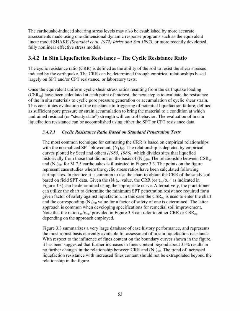
The earthquake-induced shearing stress levels may also be established by more accurate assessments made using one-dimensional dynamic response programs such as the equivalent linear model SHAKE (Schnabel et al. 1972; Idriss and Sun 1992), or more recently developed, fully nonlinear effective stress models.

3.4.2 In Situ Liquefaction Resistance – The Cyclic Resistance Ratio

The cyclic resistance ratio (CRR) is defined as the ability of the soil to resist the shear stresses induced by the earthquake. The CRR can be determined through empirical relationships based largely on SPT and/or CPT resistance, or laboratory tests.

Once the equivalent uniform cyclic shear stress ratios resulting from the earthquake loading (CSReq) have been calculated at each point of interest, the next step is to evaluate the resistance of the in situ materials to cyclic pore pressure generation or accumulation of cyclic shear strain. This constitutes evaluation of the resistance to triggering of potential liquefaction failure, defined as sufficient pore pressure or strain accumulation to bring the material to a condition at which undrained residual (or “steady state”) strength will control behavior. The evaluation of in situ liquefaction resistance can be accomplished using either the SPT or CPT resistance data.

3.4.2.1 Cyclic Resistance Ratio Based on Standard Penetration Tests

The most common technique for estimating the CRR is based on empirical relationships with the normalized SPT blowcount, (N1)60. The relationship is depicted by empirical curves plotted by Seed and others (1985, 1986), which divides sites that liquefied historically from those that did not on the basis of (N1)60. The relationship between CSReq and (N1)60 for M 7.5 earthquakes is illustrated in Figure 3.3. The points on the figure represent case studies where the cyclic stress ratios have been calculated following earthquakes. In practice it is common to use the chart to obtain the CRR of the sandy soil based on field SPT data. Given the (N1)60 value, the CRR (or τav/σvo′ as indicated in Figure 3.3) can be determined using the appropriate curve. Alternatively, the practitioner can utilize the chart to determine the minimum SPT penetration resistance required for a given factor of safety against liquefaction. In this case the CSReq is used to enter the chart and the corresponding (N1)60 value for a factor of safety of one is determined. The latter approach is common when developing specifications for remedial soil improvement. Note that the ratio τav/σvo′ provided in Figure 3.3 can refer to either CRR or CSReq, depending on the approach employed.

Figure 3.3 summarizes a very large database of case history performance, and represents the most robust basis currently available for assessment of in situ liquefaction resistance. With respect to the influence of fines content on the boundary curves shown in the figure, it has been suggested that further increases in fines content beyond about 35% results in no further changes in the relationship between CRR and (N1)60. The trend of increased liquefaction resistance with increased fines content should not be extrapolated beyond the relationship in the figure.

53

Figure 3.3: Empirical Relationship between the Cyclic Stress Ratio Initiating Liquefaction and (N1)60 Values for Silty Sands in M 7.5 Earthquakes

(Youd and Idriss 1997; after Seed et al. 1979)

The corrected blow count, (N1)60 is commonly determined from the measured standard penetration resistance, Nm, but may also be determined from CPT resistance data using standard correlations to estimate Nm values. With the development of reliable CPT-based evaluation procedures, this conversion of CPT data to equivalent SPT data for use in the CRR determination is no longer recommended (this is discussed in subsequent paragraphs). The value for (N1)60 is calculated from Nm as follows:

� � mm

N1 N60

ERCN ��

���

��60 (3-3)

where CN is a factor that corrects Nm to an effective overburden pressure of 98 kPa (1 ton/ft2), and ERm is the measured hammer energy ratio or efficiency which is defined as the percent of theoretical free-fall hammer energy that is actually transferred to the

54

drill rod during hammer impact. In order to utilize world-wide data, the recommendation is to normalize all values to a utilized energy of 60%. A table for this normalization is given by Seed and others (1985).

Because the blowcount is a function of the effective confining stress, and confining stress is a function of depth, the N-value is normalized by the factor CN to an effective overburden pressure of 98 kPa. An approach proposed by Liao and Whitman (1985) suggests that the following equation can be used to estimate CN:

5.0

���

����

��

'1Cvo

N� (3-4)

where σvo′ is expressed in tons/ft2. If Dr must be estimated, then the following approximate relationship can be used:

0.0046 (Dr)2 = (N1)60 (3-5)

There are several corrections proposed to account for the many other variables involved with the SPT, such as short lengths of drill rod, differences in sampling tube design, diameter of bore hole, frequency of hammer drop, etc. These corrections, as well as the recommended “standardized” SPT equipment and procedures, are discussed in greater detail by Seed and others (1985).

The relationship between (N1)60 and the equivalent uniform cyclic stress ratio necessary to cause liquefaction (the boundary curves in Figure 3.3) can be applied for earthquakes with a magnitude other than M 7.5 by the application of the Magnitude Scaling Factor (MSF). The long-standing MSF values of Seed and Idriss (1982) have been updated based on recent investigations (Youd and Idriss 1997). The most recently recommended MSF values are shown graphically in Figure 3.4. The value of CRR determined from Figure 3.3 can be corrected to account for the magnitude of interest by means of the following formula:

CRR (M) = CRR (M 7.5) (MSF) (3-6)

55

Figure 3.4: Magnitude Scaling Factors Derived by Various Investigators (Youd and Idriss 1997)

Seed and Harder (1990) suggest correcting the CRR value for two additional factors, Kσ and Kα, which are used to account for the influence of soil depth and the presence of static shear stress (sloping ground condition), respectively. The factor Kσ is used to correct CRR for the effects of large overburden pressures that are typically found beneath embankments, dams and deep fills. As the overburden pressure increases, the CSR required to cause liquefaction (CSRL) effectively decreases. For liquefiable materials at shallow depths (less than 12 m) where most lateral spreads occur, the Kσ correction factor is generally near 1.0 (Figure 3.5). Recent recommendations pertaining to the correction factors have been summarized by Youd and Idriss (1997).

56

Figure 3.5: Minimum Values for Kσ Recommended for Clean Sands, Silty Sands and Gravels (Youd and Idriss 1997, after Seed and Harder 1990)

An additional correction has been proposed for the simplified liquefaction procedure. The second correction factor, Kα, is used to account for conditions other than level ground, such as the case with bridge embankments. For level ground conditions, there are no static driving shear stresses acting on a horizontal plane in the soil. When sloping ground conditions exist, the generation of pore pressures and accumulation of shear strains under cyclic loading can be significantly affected by the presence of static driving shear stresses and must be accounted for in analysis of liquefaction resistance. Recent studies have shown that the presence of static driving shear stresses in loose, contractive soils can decrease the liquefaction resistance of the soil (Seed and Harder 1990). To account for the effects of static driving shear stresses, the following equation should be used:

CSRL (α=α) = CSRL (α=0) Kα (3-7)

A relationship between Kα and α is presented in Figure 3.6. This relationship has been discussed in several workshops (Youd and Idriss 1997) and the current consensus recommendation is that the use of this factor is not advisable.

57

Figure 3.6: Correction Factors K

� for Static Shear Ratios � (Marcuson et al. 1992)

In summary, the equivalent uniform CSR necessary to cause or trigger liquefaction can be determined based on the knowledge of six factors:

� the (N1)60 value, � the fines content, � the in situ static shear stress, � the initial effective overburden stress, � the earthquake magnitude or number of equivalent loading cycles, and � the peak horizontal acceleration at the ground surface.

3.4.2.2 Cyclic Resistance Ratio Based on Cone Penetration Tests

As an alternative to the use of SPT N-values, CPT tip resistance (qc) values may be used as a basis for evaluation of in situ liquefaction resistance. In the “Proceedings of the NCEER Workshop on Evaluation of Liquefaction Resistance of Soils” (Youd and Idriss 1997), workshop participants were unable to reach a consensus on a single, preferred CPT-based criterion for evaluating liquefaction resistance. In light of this assessment, the methods proposed by Robertson and Wride (1997a, b) and Olsen (1997) will be outlined here. It has been found on several projects that the CRR values calculated by CPT-based methods are, on average, smaller and more conservative than SPT-based methods.

58

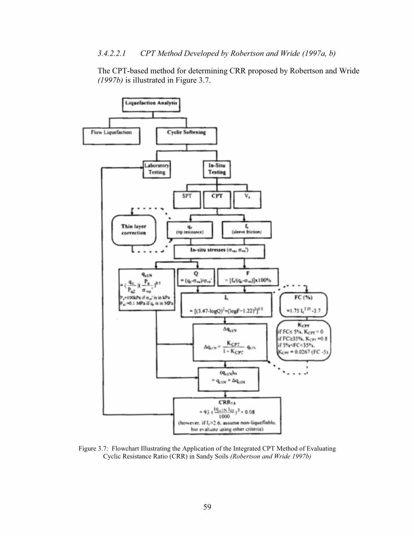
3.4.2.2.1 CPT Method Developed by Robertson and Wride (1997a, b)

The CPT-based method for determining CRR proposed by Robertson and Wride (1997b) is illustrated in Figure 3.7.

Figure 3.7: Flowchart Illustrating the Application of the Integrated CPT Method of Evaluating Cyclic Resistance Ratio (CRR) in Sandy Soils (Robertson and Wride 1997b)

59

The procedure can be easily performed by means of spreadsheet manipulations. The first step involves modifying the measured cone resistance (qc) and sleeve friction (fs). This includes normalizing and correcting the measured data for overburden stress to yield qc1N. The value qc1N is calculated by employing equation 3-8a. The sleeve friction measured by the cone is also normalized by use of Equation 3-8b. Note that these corrections yield dimensionless values for tip resistance and sleeve friction.

2

1

a

c

Pq

'σP

Pqq

0.5

vo

a

a2

ccIN ���

�

����

����

����

�� (3-8a)

� �%100*

σqf

Fvoc

s���

����

�

��

(3-8b)

where: qc = measured, uncorrected tip penetration resistance � �vo′ = vertical effective stress � �vo = total vertical stress Pa = reference pressure of 100 kPa in same units as σvo′; Pa = 100

kPa if σvo′ is in kPa. Pa2 = reference pressure of 100 kPa in same units as qc; Pa2 = 0.1

MPa if qc is in MPa. fs = CPT sleeve friction stress

A third CPT-based parameter, Q, is also required for this procedure. The measured cone tip resistance is normalized to yield a second dimensionless penetration resistance using Equation 3-9.

� �'σσqQ

vo

voc �

� (3-9)

where: qc and σvo′ have been previously defined, and σvo = total overburden stress

A chart (Figure 3.8) relating Q and F to the soil behavior type allows for approximate soil classification based on the normalized CPT data.

60

1. Sensitive, fine grained 6. Sands – clean sand to silty sand 2. Organic soils – peats 7. Gravelly sand to dense sand 3. Clays – silty clay to clay 8. Very stiff sand to clayey sand* 4. Silt Mixtures – clayey silt to silty clay 9. Very stiff, fine grained* 5. Sand Mixtures – silty sand to sandy silt

* Heavily overconsolidated or cemented

Figure 3.8: Normalized CPT Soil Behavior Type Chart (after Robertson and Wride 1997a, b)

An empirical Soil Behavior Type Index, Ic, has been proposed for use in estimating the fines content of the soil from the Q and F values. The Soil Behavior Type Index is defined in Equation 3-10. This index parameter is used to convert the measured CPT tip resistance to the value that would be expected for an equivalent clean sand. Ranges of Ic for the soil types illustrated in Figure 3.8 are provided in Table 3.6. Once Ic has been determined, the fines content of the soil can be estimated by an empirical relationship based on the soil zones in Figure 3.8.

(3-10) � � �� �0.522 1.22loglog3.47 ���� FQI c �

61

Table 3.6: Boundaries of Soil Behavior Type (Robertson and Wride 1997a, b) Soil Behavior Type Index, Ic Zone Soil Behavior Type

Ic < 1.31 7 Gravelly sand to dense sand 1.31 < Ic < 2.05 6 Sands: clean sand to silty sand 2.05 < Ic < 2.60 5 Sand Mixtures: silty sand to sandy silt 2.60 < Ic < 2.95 4 Silt Mixtures: clayey silt to silty clay 2.95 < Ic < 3.60 3 Clays: silty clay to clay

Ic > 3.6 2 Organic soils: peats

The simplified relationship that has been proposed for use in practice is provided in Equation 3-11. It is recommended that this formula should be amended, where needed, to fit the results of site- or region-specific geotechnical investigations. Versions of this basic equation, modified with site-specific data have been proven to be very reliable for use in liquefaction studies.

(3-11) 3.7)1.75(I(%) FCContent, Fines ��3.25

c

Figure 3.9 shows that for a given value of qc1N, the CRR increases with increasing fines content; therefore, it is necessary to correct the in situ value of qc1N to an equivalent clean sand value, (qc1N)cs prior to the calculation of the cyclic resistance ratio. This correction is achieved using the fines-dependent correction factor, KCPT. The equivalent clean sand normalized CPT tip resistance is given as:

(3-12) cscINCPTcIN )q(Kq ��

where: ∆qc1N = CPT tip correction for silty sands (qc1N)cs = equivalent clean sand normalized CPT tip resistance (this is

equal to qc1N + ∆qc1N) qc1N = measured tip resistance, corrected for overburden and

normalized KCPT = 0 for FC <5% = 0.0267(FC – 5), for 5% < FC < 35% = 0.80 for FC > 35%.

Thus the CPT correction can be expressed as a function of the measured data with Equation 3-13.

)q()K-(1

Kq cINCPT

CPTcIN �

�

���

��� (3-13)

62

Figure 3.9: CPT-Based Curves for Various Values of Soil Behavior Index, Ic

(Robertson and Wride 1997a) Note: FC=Fines Content.

As outlined by Robertson and Wride (1997b), Equation 3-13 can be used to obtain the equivalent clean sand normalized penetration resistance, (qc1N)cs, directly from the measured CPT data. In the final step of the procedure, the CRR estimated using the clean sand curve shown in Figure 3.8 is estimated for ground motions due to a magnitude 7.5 earthquake (Equation 3-14).

0.081000q93CRR cIN ���

���

��

3)( cs (3-14)

where: (qc1N)cs is in the range of 30 < (qc1N)cs < 160.

The CRR is scaled for the design-level earthquake motion(s) using the appropriate MSFs (Figure 3.4). The recommended design chart is shown in Figure 3.10. It should be noted that for Ic > 35% (i.e. FC > 35%) the soil is considered to be non-liquefiable by Robertson and Wride. They add that this general guideline should be checked using independent methods of analysis. Recent laboratory investigations by the author and his students have demonstrated that low- to moderate-plasticity silts located along the Interstate 5 corridor in the Portland-

63

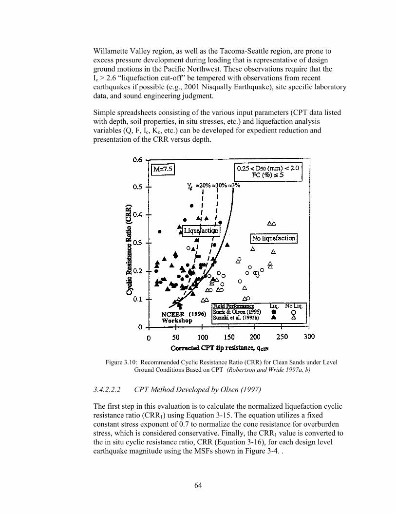
Willamette Valley region, as well as the Tacoma-Seattle region, are prone to excess pressure development during loading that is representative of design ground motions in the Pacific Northwest. These observations require that the Ic > 2.6 “liquefaction cut-off” be tempered with observations from recent earthquakes if possible (e.g., 2001 Nisqually Earthquake), site specific laboratory data, and sound engineering judgment.

Simple spreadsheets consisting of the various input parameters (CPT data listed with depth, soil properties, in situ stresses, etc.) and liquefaction analysis variables (Q, F, Ic, Kc, etc.) can be developed for expedient reduction and presentation of the CRR versus depth.

Figure 3.10: Recommended Cyclic Resistance Ratio (CRR) for Clean Sands under Level

Ground Conditions Based on CPT (Robertson and Wride 1997a, b)

3.4.2.2.2 CPT Method Developed by Olsen (1997)

The first step in this evaluation is to calculate the normalized liquefaction cyclic resistance ratio (CRR1) using Equation 3-15. The equation utilizes a fixed constant stress exponent of 0.7 to normalize the cone resistance for overburden stress, which is considered conservative. Finally, the CRR1 value is converted to the in situ cyclic resistance ratio, CRR (Equation 3-16), for each design level earthquake magnitude using the MSFs shown in Figure 3-4. .

64

� �

)(0.0016)(0.028)(0.170.0250.00128 32

0.71 fff

v

c RRR'σ

qCRR �������

����

� (3-15)

where: � � 70.

v

c

'q

�

= generalized normalized cone resistance

CRR = normalized liquefaction cyclic resistance ratio Rf = calculated friction ratio (percentage) qc = CPT measured cone resistance (in atm units) �v′ = vertical effective stress (in atm units)

(3-16) 1CRRMSFCRR ��

A direct comparison of the two CPT methods is made in the design application contained in Chapter 8.

3.4.2.3 Cyclic Resistance Ratio from Laboratory Tests

Cyclic tests (triaxial, simple shear, torsional shear) can be performed to determine the cyclic behavior of silty and fine sandy soils. Undrained, stress- or strain-controlled tests consisting of uniform sinusoidal loading are commonly performed. With respect to common stress-controlled cyclic triaxial tests, loads are applied to the specimens until a specified axial strain or number of loading cycles is reached. In numerous laboratory studies of sandy soils, axial strains of 5% are generally achieved when the specimen first reaches full liquefaction (defined as zero effective stress). An equivalent way of defining full liquefaction is based on the pore pressure ratio (ru = 100%), as defined in Equation 3-17. Note that 5% axial strain and ru criteria for defining the onset of liquefaction do not always occur in the same number of load cycles. The differences observed in the number of cycles are generally minor for sandy soils, but increase with fines content due to the relative low permeability of fine grained soils and testing limitations in measuring excess pore pressures generated with rapid loading.

100%*3σ'

∆uru � (3-17)

The CRR values obtained from laboratory tests must be corrected to field CRR values through the use of two correction factors. The first factor, cr, accounts for the fact that cyclic triaxial compression and cyclic simple shear tests impose different loadings. The cyclic simple shear tests are considered to be more representative of the field conditions with vertically propagating shear waves. In order to relate cyclic triaxial shear (CRRtx) data to cyclic simple shear (CRRss) data, the following equation has been formulated:

(3-18) txrss CRR*cCRR �

where recommended values of cr have been compiled in Table 3.7 as a function of the static lateral earth pressure coefficient (Ko).

65

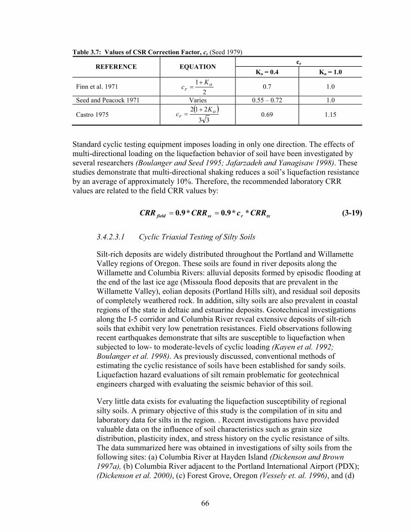
Table 3.7: Values of CSR Correction Factor, cr (Seed 1979) cr REFERENCE EQUATION

Ko = 0.4 Ko = 1.0

Finn et al. 1971 2

1 or

Kc

�

� 0.7 1.0

Seed and Peacock 1971 Varies 0.55 – 0.72 1.0

Castro 1975 � �

33212 o

rK

c�

� 0.69 1.15

Standard cyclic testing equipment imposes loading in only one direction. The effects of multi-directional loading on the liquefaction behavior of soil have been investigated by several researchers (Boulanger and Seed 1995; Jafarzadeh and Yanagisaw 1998). These studies demonstrate that multi-directional shaking reduces a soil’s liquefaction resistance by an average of approximately 10%. Therefore, the recommended laboratory CRR values are related to the field CRR values by:

(3-19) txrssfield CRRcCRRCRR **0.9*0.9 ��

3.4.2.3.1 Cyclic Triaxial Testing of Silty Soils

Silt-rich deposits are widely distributed throughout the Portland and Willamette Valley regions of Oregon. These soils are found in river deposits along the Willamette and Columbia Rivers: alluvial deposits formed by episodic flooding at the end of the last ice age (Missoula flood deposits that are prevalent in the Willamette Valley), eolian deposits (Portland Hills silt), and residual soil deposits of completely weathered rock. In addition, silty soils are also prevalent in coastal regions of the state in deltaic and estuarine deposits. Geotechnical investigations along the I-5 corridor and Columbia River reveal extensive deposits of silt-rich soils that exhibit very low penetration resistances. Field observations following recent earthquakes demonstrate that silts are susceptible to liquefaction when subjected to low- to moderate-levels of cyclic loading (Kayen et al. 1992; Boulanger et al. 1998). As previously discussed, conventional methods of estimating the cyclic resistance of soils have been established for sandy soils. Liquefaction hazard evaluations of silt remain problematic for geotechnical engineers charged with evaluating the seismic behavior of this soil.

Very little data exists for evaluating the liquefaction susceptibility of regional silty soils. A primary objective of this study is the compilation of in situ and laboratory data for silts in the region. . Recent investigations have provided valuable data on the influence of soil characteristics such as grain size distribution, plasticity index, and stress history on the cyclic resistance of silts. The data summarized here was obtained in investigations of silty soils from the following sites: (a) Columbia River at Hayden Island (Dickenson and Brown 1997a), (b) Columbia River adjacent to the Portland International Airport (PDX); (Dickenson et al. 2000), (c) Forest Grove, Oregon (Vessely et. al. 1996), and (d)

66

Tacoma, Washington (Dickenson and Brown 1997b). Additional data has been gleaned from laboratory testing of reconstituted specimens at Oregon State University (Brown, in preparation). The geotechnical characterization for these sites included mud rotary borings, thin-wall tube samples in the low- to high-plasticity silts, penetration resistances provided by SPT and CPT, as well as limited shear wave velocity and pore pressure data (excess pore pressures during cone advance and pore pressure dissipation in the fine sands and silts). Conventional cyclic triaxial and simple shear equipment was employed and modified with Bender elements for obtaining the shear wave velocity of the triaxial specimens, and with enhanced volume change instrumentation.

It is well known that the results of cyclic triaxial data are not strictly representative of field behavior due to testing limitations, such as boundary conditions, stress paths, and uniform uni-directional loading. Additionally, the low to non-plastic nature of these soils makes undisturbed sampling very difficult. Any technique short of controlled ground freezing and coring would be expected to disturb the soil fabric and densify the material, thereby altering its behavior and its tendency to generate pore pressure. Determining the magnitude of such alterations is arduous. However, the qualitative nature of the effect is more predictable. For loose, saturated deposits with very low to no cohesion, the effects of sample disturbance densifies the samples and increases their liquefaction resistance during laboratory testing. For this reason, laboratory tests would likely overestimate the liquefaction resistance of the in situ soil to some degree. The cyclic testing does, however, yield useful data on the liquefaction resistance of predominantly silty soils relative to sandy soils tested using the same equipment. This data is considered particularly useful for demonstrating how the liquefaction behavior of the silts varies from that of sand, for which current empirical procedures for assessing liquefaction hazards are well established.

The results of cyclic triaxial tests on silty soils from various sites in the Pacific Northwest are presented in Figure 3.11. Cyclic triaxial tests conducted on soils from the Puyallup River near Tacoma, Columbia River near Portland, and Fern Hill, Oregon are presented to demonstrate the cyclic resistance curves as a function of OCR. The data in Figure 3.11 clearly demonstrates the influence of stress history on the soil’s liquefaction resistance. This effect should be accounted for in hazard analyses involving overconsolidated soils. The geotechnical properties of the samples are provided in Table 3.8. The data for relatively undisturbed specimens of silt soils from the Pacific Northwest provided in Table 3.8 are augmented with test results for reconstituted specimens, as well as the results of similar testing performed on other low plasticity silts (i.e., Bonnie silt and a silt from France). This data highlights the range in cyclic resistance obtained for the various silts using cyclic triaxial equipment. The data provided in Table 3.8 also demonstrates the influence of sample preparation on the measured behavior of the specimens. For example, the cyclic resistance of he Tacoma silt represent tests performed on high quality specimens from the field and on specimens reconstituted from a slurry and consolidated to stresses equivalent to those in the field. Although the specimens were consolidated to the same stresses

67

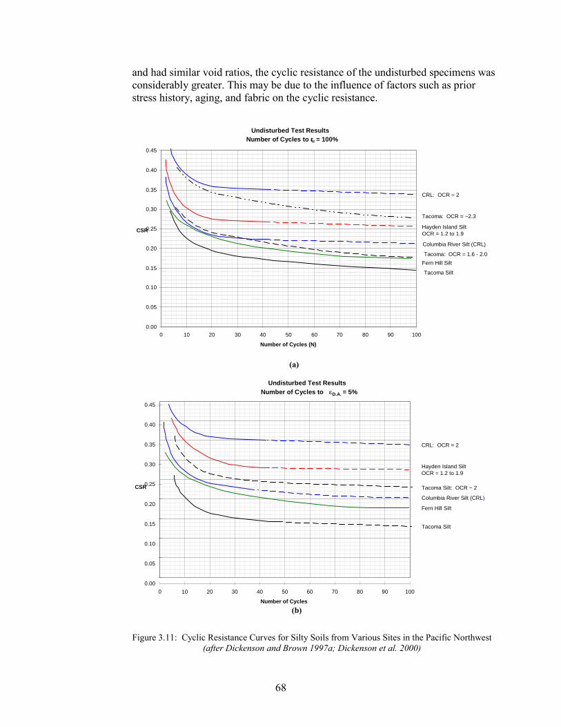
and had similar void ratios, the cyclic resistance of the undisturbed specimens was considerably greater. This may be due to the influence of factors such as prior stress history, aging, and fabric on the cyclic resistance.

Undisturbed Test Results

Number of Cycles to ru = 100%

0.00

0.05

0.10

0.15

0.20

0.25

0.30

0.35

0.40

0.45

0 10 20 30 40 50 60 70 80 90 100 Number of Cycles (N)

CSR WSDOT: PTR I/C

Hayden Island

Fern Hill

Tacoma Silt

Tacoma: OCR = 1.6 - 2.0

Columbia River Silt (CRL)

Tacoma: OCR = ~2.3

CRL: OCR = 2

Fern Hill Silt

Hayden Island SiltOCR = 1.2 to 1.9

(a)

(b)

Undisturbed Test ResultsNumber of Cycles to �D.A. = 5%

0.00

0.05

0.10

0.15

0.20

0.25

0.30

0.35

0.40

0.45

0 10 20 30 40 50 60 70 80 90 100 Number of Cycles

CSR

Tacoma Silt

Tacoma Silt: OCR ~ 2

Fern Hill Silt

Columbia River Silt (CRL)

Hayden Island SiltOCR = 1.2 to 1.9

CRL: OCR = 2

Figure 3.11: Cyclic Resistance Curves for Silty Soils from Various Sites in the Pacific Northwest

(after Dickenson and Brown 1997a; Dickenson et al. 2000)

68

Table 3.8: Influence of OCR on the Cyclic Stress Ratio Required to Cause Liquefaction and Large Strains in Silt Specimens.

Atterberg LimitsResults Percent Fines CRRN = 20

2 Sample

Water Content

(%) LL PI #200 Sieve 2 µm

Void Ratio OCR ru =

100% εD.A. =5%3

εS.A.=5%3

0.65 – 1.06 1 0.19 0.17 0.21 0.89 – 1.15 1.5 – 2.0 0.24 0.28 0.39 Undisturbed

Tacoma silt 27 - 48 - NP 27 – 100 4 – 22 0.88 2.0 – 2.5 ~0.34 - ~0.39

Undisturbed Hayden Island

silt 38 - 62 - 1.03 – 1.12 1.6 – 1.9 0.28 0.31 0.33

1.73 1.0 0.23 0.25 - Undisturbed CRL silt 38 - 62 31 – 54 1 – 14 2 – 71

1.03 – 1.12 2.0 0.36 0.37 - Undisturbed Fern Hill silt - - ≤ 2 80 5 - 1 0.24 0.24 0.24

0.78 - 0.82 1 0.17 0.17 0.17 Reconstituted Tacoma Silt 30 – 31 - - - -

0.8 1.5 – 2.0 0.24 0.24 0.25 0.60 – 0.82 1.0 0.22 0.20 0.23 Reconstituted

Corvallis Silt 22 – 30 33 – 38 7 – 11 98 – 100 24 – 290.61 – 0.79 1.5 0.27 0.24 0.28 0.83 – 0.95 1.0 ~0.261 ~0.241 ~0.251Reconstituted

Adair Silt 33 - 35 44 – 45 8 – 9 99 – 100 53 – 570.93 – 0.96 1.5 - 2.0 ~0.421 ~0.411 ~0.411

Reconstituted Bonnie silt 29 15 90 – 93 6 - 7 0.79 – 0.80 1 0.281 0.27 0.27

Undisturbed French Silt

Site 1 19 - 26 22 – 32 5 – 8 - 19 - 21 0.47 – 0.65 - 0.26 –

0.32 0.23 – 0.33 -

Undisturbed French Silt

Site 2 28 - 42 30 - 50 7 – 15 - 17 - 28 - ~0.27 ~0.29 -

NOTES 1 Extrapolated value. 2 CRRN=20 is the cyclic stress ratio required to reach the specified pore pressure ratio (ru) or strain (�S.A. or �D.A.) in 20

load cycles. 3 εD.A. is the double amplitude axial strain and εS.A. is the single amplitude axial strain.

The laboratory results presented in Figure 3.11 demonstrate that although the silts are capable of liquefying during cyclic triaxial testing, the CSR required to induce full liquefaction in the number of loading cycles of interest (roughly 10 to 50 cycles) are somewhat higher than those reported for loose clean sands under equivalent loading conditions. It is interesting to note the influence of stress history on the cyclic resistance of the silt. The effect of the overconsolidation ratio (OCR) on the cyclic liquefaction resistance has been noted in several studies of sandy soils (Yamazaki et al. and Ishihara, in PHRI 1997). Data from laboratory testing of a silty sand demonstrates that the increase in cyclic resistance increases with the square root of the overconsolidation ratio (Figure 3.12). The data is plotted as (τl/σc′)N= 20 cycles, where τl is the uniform cyclic shear stress required to case liquefaction in 20 cycles of loading (i.e., N = 20), and σc′ is the consolidation pressure prior to cyclic loading.

69

Figure 3.12: Influence of Overconsolidation Ratio on the Cyclic Resistance of a Marine Sand (Yamazaki et al in PHRI 1998)

It has been shown that the influence of OCR is a function of the fines content, and generally increases with increasing fines (Figure 3.13). The increase in the effect of stress history on the CRR for silts is due in part to the fact that these materials are more compressible than sandy soils. It has been determined, based on the work of Dickenson and others, that the increase in cyclic resistance increases to the exponent of 0.7 to 0.8. A value of 0.75 is recommended at this time. This value is greater than the value of 0.5 recommended for sandy soils. The significance of this finding is that over-consolidated silts are considered to be less susceptible to cyclically induced pore pressure generation than silty- or clean-sands having the same OCR.

The fines content (percent by weight passing the No. 200 sieve) of the silts tested by Dickenson varied between 65% and 100% with most of the specimens above 90%. The increase in liquefaction resistance found in the Columbia River and Tacoma specimens is consistent with the work of Ishihara (Figure 3.13). This is a potentially important factor in light of the stress history profiles observed at most sites along the I-5 corridor. The cyclic resistance data provided in Figures 3.11a and 3.11b are used directly in the liquefaction hazard evaluation presented in Chapter 8.

70

Figure 3.13: Influence of Fines Content and Overconsolidation Ratio on the Cyclic

Resistance of Sands and Silts (Ishihara in PHRI 1998)

In addition to the stress history, the plasticity of the fines must also be evaluated prior to establishing the liquefaction susceptibility of the deposit. This influence has been addressed by Ishihara (1993, 1996). As demonstrated in Figure 3.14, an increase in the PI of the soil tends to increase its resistance to liquefaction.

Figure 3.14: Effects of Plasticity Index on Cyclic Strength of Silty Soils (Ishihara 1996)

71

To estimate CRR values for use in liquefaction hazard evaluations, the number of uniform loading cycles anticipated for each design-level earthquake is required. Recent data relating the number of uniform cycles to earthquake magnitude, shown in Figure 3.15, was utilized (Liu and Stewart 1999). It should be noted that the curves were extrapolated for magnitudes greater than 7.0. Given the cyclic resistance curves (Figures 3.11a and 3.11b) and the number of uniform loading cycles for the scenario earthquakes (Figure 3.15), the CRR can be estimated. This procedure is applied for a site along the Columbia River in Chapter 8.

0

5

10

15

20

25

30

35

40

45

50

5 5.5 6 6.5 7 7.5 8 8.5

Magnitude

Equi

vale

nt N

umbe

r of U

nifo

rm C

ycle

s

9

Subduction Zone (d = 85 km)

Crustal (d = 8 km)

Seed and Idriss (1975)

Figure 3.15: Variation of Equivalent Uniform Loading Cycles with Earthquake Magnitude (Liu and Stewart 1999)

3.4.3 Factor of Safety and Degree of Cyclic Pore Pressure Generation

The factor of safety against the triggering of liquefaction is calculated by the following equation.

FSL = CRR6 / CSReq (3-20)

This factor of safety can be used to estimate the excess pore pressures generated during seismic loading. Figure 3.16 shows a plot of the Residual Excess Pore Pressure Ratio (ru = ∆u/σvo

′) based on laboratory test data for level ground conditions (α = 0�). Considerable judgment should be used in the application of these excess pore pressures in effective stress analyses. It is recommended that a range of likely ru values be selected from the chart and the sensitivity of the excess pore pressure on the resulting hazard evaluation be determined.

72

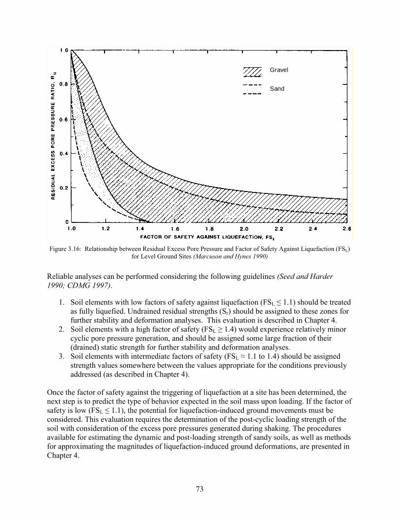
Gravel

Sand

Figure 3.16: Relationship between Residual Excess Pore Pressure and Factor of Safety Against Liquefaction (FSL)

for Level Ground Sites (Marcuson and Hynes 1990)

Reliable analyses can be performed considering the following guidelines (Seed and Harder 1990; CDMG 1997).

1. Soil elements with low factors of safety against liquefaction (FSL ≤ 1.1) should be treated as fully liquefied. Undrained residual strengths (Sr) should be assigned to these zones for further stability and deformation analyses. This evaluation is described in Chapter 4.

2. Soil elements with a high factor of safety (FSL ≥ 1.4) would experience relatively minor cyclic pore pressure generation, and should be assigned some large fraction of their (drained) static strength for further stability and deformation analyses.

3. Soil elements with intermediate factors of safety (FSL ≈ 1.1 to 1.4) should be assigned strength values somewhere between the values appropriate for the conditions previously addressed (as described in Chapter 4).

Once the factor of safety against the triggering of liquefaction at a site has been determined, the next step is to predict the type of behavior expected in the soil mass upon loading. If the factor of safety is low (FSL ≤ 1.1), the potential for liquefaction-induced ground movements must be considered. This evaluation requires the determination of the post-cyclic loading strength of the soil with consideration of the excess pore pressures generated during shaking. The procedures available for estimating the dynamic and post-loading strength of sandy soils, as well as methods for approximating the magnitudes of liquefaction-induced ground deformations, are presented in Chapter 4.

73

4.0 POST-LIQUEFACTION SOIL BEHAVIOR

4.1 INTRODUCTION

Common methods for evaluating liquefaction potential were outlined in Chapter 3. Although these methods can be used to indicate the triggering of liquefaction, they do not describe the behavior of the soil after this state has been reached. As the cyclically-induced excess pore pressures build up in the soil, it experiences a dramatic reduction in stiffness and strength. This occurs as the excess pore pressure increases; therefore, it is not necessary for the soil to reach a state of liquefaction (ru = 100%) for it to be potentially hazardous. Ground failures associated with liquefied soil include:

1. flow failures of sloping ground or free-face conditions; 2. limited, yet excessive, deformations of sloping ground and free-face conditions (termed

lateral spreading); 3. bearing capacity failures of shallow foundations; 4. increased lateral earth pressure on walls leading to large displacements; 5. loss of passive soil resistance against walls, anchors, laterally loaded piles; and 6. excessive ground settlement.

Liquefaction-related ground failures have been a primary source of damage to highway structures during recent earthquakes. Excessive deformations of pavements, approach fills, pile foundations, and bridge substructures result in the loss of bridge operation. The engineering parameters utilized in conventional limit equilibrium analyses must be assessed. The substantial change in engineering properties of soils throughout the cyclic loading and liquefaction process is complex; however, simplified procedures have been developed for estimating the post-cyclic loading, or post-liquefaction behavior of cohesionless soils. Recently developed methods for evaluating the shear strength, post-loading volume change, and magnitude of lateral spreading are discussed in this chapter.

4.2 POST-CYCLIC STRENGTH OF SANDS AND SILTS

In order to assess the seismic stability of earth structures and foundations, it is necessary to estimate the shear strength of the soil during and after the seismic loading. The potential loss of soil shear strength is a function of the excess pore pressures that are developed during shaking. The following categories delineate the various stages of soil shear strength reduction due to excess pore pressure generation. The stages are defined by the factor of safety against liquefaction determined using one or more of the procedures outlined in Chapter 3. While theoretically, the value of FSL indicating full liquefaction should be 1.0, in practice, it is often recommended that a value of 1.1 be used to account for the very rapid rise in ru with FSL values less than 1.1. The use of 1.1 for “liquefied soil” provides appropriate conservatism to the analysis.

75

� FSL > 1.4: Excess pore pressure generation is considered negligible and the soil does not experience an appreciable reduction in shear strength (CDMG 1997). In this case, the drained shear strength is computed using the standard Mohr-Coulomb strength equation.

� 1.0 < FSL < 1.4: Partial excess pore pressure generation will have an effect on soil strength and should be addressed. The magnitude of the pore pressure generation is a function of FSL and soil type (Marcuson et al. 1990).

� FSL < 1.0: Soils are expected to experience full pore pressure generation and residual undrained shear strengths should be applied (Stark et al. 1997).

The latter two cases involving the generation of significant excess pore pressures are particularly relevant and are discussed in the following sections.

4.2.1 Partial Excess Pore Pressure Generation (1.0 < FSL <1.4)

As illustrated by the relationship between the excess pore pressure ratio (ru) and the factor of safety against liquefaction (FSL) for both gravel and sand (Figure 3.16), the relatively rapid increase in ru for FSL less than 1.4 will lead to an associated reduction in soil strength. A common method for reducing the static strength to account for partial pore pressure generation utilizes the Mohr-Coulomb shear strength equation for cohesionless soils (Equation 4-1). The vertical effective stress is calculated at the elevation of interest for hydrostatic, pre-earthquake conditions. The post-cyclic strength is then calculated using a reduced vertical effective stress that accounts for the excess pore pressure generation and using the static effective friction angle (�′static). Next, a reduced effective friction angle (�′equivalent) is determined using the post-cyclic shear strength, the initial vertical effective stress, and �′static. Following this process, Equation 4-2 was derived directly relating �′equivalent to ru and �′static that is independent of the in situ vertical effective stress (Ebeling and Morrison 1993). Therefore, in soil layers that experience pore pressure generation, the static shear strength of the soil is reduced using a residual effective friction angle, as opposed to reducing the vertical effective stress. This modification is required because of the inability of standard slope stability computer programs to directly account for excess pore pressure generation.

(4-1) 'tanφσ'τ n�

(4-2) � �� �staticuequivalent tanφrarctanφ' �� 1

4.2.2 Full Liquefaction (FSL < 1)

The shear strength of liquefied soils has been an area of considerable interest over the past decade. This topic was the focus of a recent workshop at which investigators evaluated the procedures for estimating the strength of sandy soils following liquefaction (Stark et al. 1998). Three approaches have been employed for evaluating the post-cyclic strength of a liquefied soil: (1) direct investigation by means of laboratory testing, (2) the comparison of in situ soil properties based largely on penetration resistance with undrained, or critical strengths back-calculated from case histories of failure, and (3) estimation of undrained strength ratios (undrained strength divided by the pre-earthquake vertical effective stress) back-calculated from

76

case histories of failure. The shear strength of liquefied soil has been described in the literature as steady state strength, residual strength, and critical strength. For the sake of clarity, the term “residual strength” (denoted as Sr) will be used exclusively in this chapter. The symbols found in subsequent figures, equations, and tables will retain the notation found in the original references. The following sections review these approaches and make recommendations for their use.

4.2.2.1 The Strength of Liquefied Sand from Laboratory Testing

The steady state methodology discussed in Section 3.3 has been widely used in practice for estimating post-cyclic shear strengths. It is based on laboratory testing of high quality, undisturbed samples combined with the necessary corrections to laboratory-measured undrained residual strengths in order to develop estimates of in situ undrained residual strengths. These steady-state analyses have been the subject of considerable research over the past decade, and several limitations have been identified. Issues have been raised, such as sampling disturbance, variability in liquefaction behavior due to the preparation techniques, boundary conditions and stress paths employed in laboratory tests, the corrections required for applying this data to field conditions, and an inherent non-conservatism of laboratory-based procedures for estimating the in situ undrained residual strengths (Seed and Jong 1987; Marcuson et al. 1990). Accordingly, the use of this approach should be tempered by the results of complementary methods for evaluating residual strengths of liquefied sand.

Laboratory tests have been used to estimate undrained strength ratios for sands and silty sands (Ishihara 1993, 1996; Baziar and Dobry 1995; Amini and Qi 2000). These studies provide valuable summaries of available data and demonstrate that undrained strength ratios obtained in the laboratory for loose sands and silty sands (Sr/σ′c ≈ � 0.1 to 0.2, where σ′c is the effective consolidation stress) compare favorably with the values back-calculated from case histories of ground failure. The influence of the plasticity index on this relationship is shown in Figure 4.1.

Figure 4.1: Normalized Residual Strength Plotted against Plasticity Index (Ishihara 1996)

77

The post-liquefaction strength of silty soils has been investigated in the laboratory by cyclically loading the soil until ru = 100%, then monotonically loading the soil undrained. It is interesting to note that numerous investigators have found that liquefied silty sands and silts are dilative when sheared following liquefaction (Stark et al. 1997; Boulanger et al. 1998; Dickenson et al. 2000). This behavior indicates that once the soil liquefies, large strains can be mobilized at sloping sites and at large strain the strength of the soil increases. This scenario assumes that the loading is fully undrained. In light of the limitations associated with sampling cohesionless soils and laboratory testing of the post-liquefaction behavior of soil, it is not recommended that the strength gain due to dilation be incorporated into design.

4.2.2.2 The Strength of Liquefied Sand from In Situ Test Data

Recognizing the difficulties associated with laboratory testing of cohesionless soil, alternative methods have been proposed for evaluating the residual shear strength of a fully liquefied deposit. Two procedures that are commonly used are: (1) residual strength ratio methods (Stark and Mesri 1992; Baziar and Dobry 1995); and (2) a procedure which is independent of the in situ vertical effective stress (Seed and Harder 1990).

The relationship between SPT data, (N1)60, and residual shear strength (Sr) with vertical effective overburden pressure (σ′vo) for silty soil deposits developed by Baziar and Dobry (1995) is shown in Figure 4.2. The curves were developed from the back-calculation of residual shear strengths from case studies where liquefaction failures had occurred. Nearly all of the case histories were selected based on previous work by Stark and Mesri (1992). The evaluation procedure developed by Baziar and Dobry is based on the use of the SPT to evaluate the potential for large deformations during earthquakes in saturated loose sandy silt and silty sand deposits and slopes. The method is based on laboratory tests and case histories corresponding to earthquakes of less than MW 8.0. Charts relating the normalized standard penetration resistance and residual shear strength to vertical effective overburden pressure have been developed for use as screening tools in liquefaction hazard evaluations (Figure 4.2).

Figure 4.2 can be used to evaluate the large ground deformation potential during earthquakes due to shearing of saturated, non-gravelly silt-sand deposits having at least 10% fines. The figure is applicable to slopes, embankments, and level or almost level sites prone to lateral spreading. Figure 4.2 suggests that silty soils with a measured (N1)60 versus σ′vo profile plotting to the right of the chart cannot experience flow failure due to their dilative behavior, and that lateral spreading generally cannot exceed 0.3 to 1.0 m (1 to 3 ft) for earthquakes of less than MW 8.0. Figure 4.2(b) indicates that for silty deposits that have experienced large deformations or flow failures, the Sr/σ′vo ranges from about 0.04 to 0.20. The average value of Sr/σ′vo is 0.12.

78

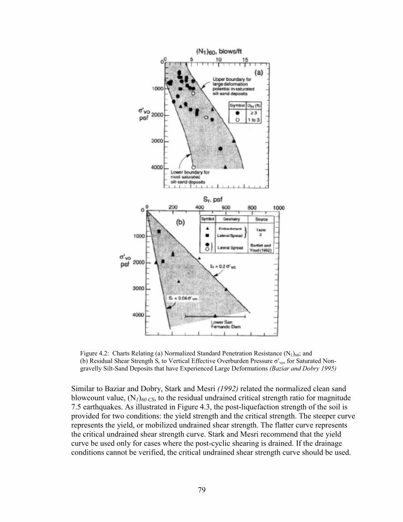
Figure 4.2: Charts Relating (a) Normalized Standard Penetration Resistance (N1)60; and (b) Residual Shear Strength Sr to Vertical Effective Overburden Pressure σ′vo, for Saturated Non-gravelly Silt-Sand Deposits that have Experienced Large Deformations (Baziar and Dobry 1995)

Similar to Baziar and Dobry, Stark and Mesri (1992) related the normalized clean sand blowcount value, (N1)60 CS, to the residual undrained critical strength ratio for magnitude 7.5 earthquakes. As illustrated in Figure 4.3, the post-liquefaction strength of the soil is provided for two conditions: the yield strength and the critical strength. The steeper curve represents the yield, or mobilized undrained shear strength. The flatter curve represents the critical undrained shear strength curve. Stark and Mesri recommend that the yield curve be used only for cases where the post-cyclic shearing is drained. If the drainage conditions cannot be verified, the critical undrained shear strength curve should be used.

79

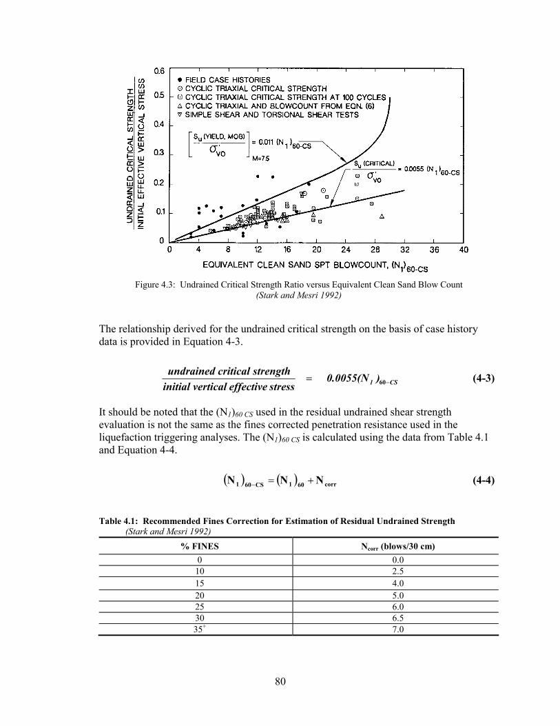
Figure 4.3: Undrained Critical Strength Ratio versus Equivalent Clean Sand Blow Count

(Stark and Mesri 1992)

The relationship derived for the undrained critical strength on the basis of case history data is provided in Equation 4-3.

CS1 )0.0055(Nstresseffective vertical initial

strength critical undrained�

� 60 (4-3)

It should be noted that the (N1)60 CS used in the residual undrained shear strength evaluation is not the same as the fines corrected penetration resistance used in the liquefaction triggering analyses. The (N1)60 CS is calculated using the data from Table 4.1 and Equation 4-4.

(4-4) � � � � corr601CS601 NNN ���

Table 4.1: Recommended Fines Correction for Estimation of Residual Undrained Strength

(Stark and Mesri 1992) % FINES Ncorr (blows/30 cm)

0 0.0 10 2.5 15 4.0 20 5.0 25 6.0 30 6.5 35+ 7.0

80

For the sake of comparison, the yield strength curve developed by Stark and Mesri provides residual strengths that are in good agreement with the results of the work by Baziar and Dobry (1995) and Ishihara (1996).

Seed and Harder (1990) analyzed a number of case studies where liquefaction-induced slides had occurred and established a correlation between equivalent clean sand blow count, (N1)60 CS, and back-calculated residual shear strength (Figure 4.4). The calculated values of (N1)60 CS are slightly different than that of Stark and Mesri because of the different fines content correction recommended by Seed and Harder (Table 4.2). The residual strength values obtained by the Seed and Harder relationship are typically more conservative than those from Stark and Mesri, even when using the curve bounding the upper limit of the data in Figure 4.4.

Figure 4.4: Relationship between Residual Strength and Corrected SPT Resistance

(Seed and Harder 1990)

Table 4.2: Recommended Fines Correction for Estimation of Residual Undrained Strength (Seed and Harder 1990)

% FINES Ncorr (blows/30 cm) 10 1.0 25 2.0 50 4.0 75 5.0

81

4.3 INTRODUCTION TO MODES OF FAILURE

Permanent ground deformations, which may occur during earthquakes as a result of increased pore water pressures and reduction of soil strength, have been a major cause of damage to structures. General modes of failure and damage of both bridge structures and other facilities can be subdivided into the following three general classes of liquefaction hazard.

1. Large-scale site instability (termed global instability) and flow failures. 2. Localized liquefaction hazard and lateral spreading. 3. Excessive deformation of retaining structures, abutments, and deep foundations.

4.3.1 Global Instability and Flow Failures

Loss of soil strength can result in global site instability, producing translational or rotational sliding, and/or flow sliding. These hazards must be addressed prior to the development of remedial soil improvement schemes. The evaluation of potential translational site instability or rotational dynamic displacement must consider dynamic loading as potential driving forces, in addition to gravitationally developed forces. These types of displacements may arise due to the following three sets of conditions.

1. Loss of soil strength resulting in overall site instability. 2. Loss of soil strength resulting in decreased slope stability, coupled with seismically-

induced dynamic inertial forces producing slope displacements. 3. Slope displacements resulting from seismically-induced dynamic inertial forces, without

pore pressure-induced soil strength loss. The evaluation of these conditions is based on conventional seismic slope stability and displacement problems. This may be accomplished using limit equilibrium slope stability analysis in conjunction with rigid body sliding block procedures (Newmark 1965; Makdisi and Seed 1978), or by performing numerical analyses. Analytical methods for evaluating seismic slope displacements have been addressed by Seed and Harder (1990) and Marcuson and others (1990).

Flow failures are the most catastrophic ground failures caused by liquefaction. They displace large masses of soil for tens of meters. The analysis often requires that the liquefaction susceptibility of the local soils be evaluated over a much larger area than just the site of interest. Relatively thin seams of liquefiable material, if both very loose and fairly continuous over large lateral areas, may serve as significant planes of weakness for overall sliding or global site instability. Flows usually develop in loose saturated sands or silts on slopes greater than three degrees. The failure of the upstream slope of the Lower San Fernando Dam during the 1971 San Fernando earthquake is a notable and well-studied example of a flow failure (Seed et al. 1975; Castro et al. 1989; Inel et al. 1993; Roth et al. 1993; Baziar and Dobry 1995; Moriwaki et al. 1998). An instructive example of the analysis of global liquefaction hazard due to flow failure has been presented by Kayen and others (1998).

82

4.3.2 Localized Liquefaction Hazard and Lateral Spreading

The three main types of localized liquefaction hazard include:

1. loss of bearing capacity beneath shallow foundations and around deep foundation piles; 2. excessive ground settlement; and 3. localized lateral displacements and lateral spreading.

The loss of soil strength can result in potential foundation bearing failure and large foundation settlements. The assessment of these potential hazards requires evaluating the liquefaction potential and the factor of safety with respect to bearing failure (Sasaki et al. 1996; Naesgaard et al. 1998). Estimating the post-cyclic strength of the soil should be determined in accordance with the methods described in Section 4.2. To evaluate the factor of safety with respect to bearing failure, conventional bearing capacity analyses should be performed using modified strengths of the foundation soils reflecting the adverse impact of cyclic pore pressure generation. Engineering judgment should be used when determining the factor of safety with respect to bearing capacity failure. It has been shown that settlements of individual footings can be highly differential in nature and can be very damaging to structures.

Hazards also are associated with lenses of liquefiable soil or by potentially liquefiable layers that underlie resistant, nonliquefiable capping layers. In situations where a few thin lenses of liquefiable soil are identified, the interlayering of liquefiable and resistant soils may serve to minimize structural damage to light, ductile structures. It may be determined that life safety and/or serviceability requirements may be met despite the existence of potentially liquefiable layers. Ishihara (1985) developed an empirical relation that provides approximate boundaries for surface damage for soil profiles consisting of a liquefiable layer overlain by a resistant surface layer (Figure 4.5). This relationship has been validated by Youd and Garris (1995) for earthquakes with magnitudes between 5.3 and 8.0. In light of the heterogeneous nature of most soil deposits and the uncertainties inherent in the estimation of ground motion parameters, it is recommended that this method of evaluation only be considered for noncritical structures.

As the excess pore pressures generated by cyclic loading dissipate by drainage, the soil is consolidating which results in ground surface settlements. Similarly, in non-saturated cohesionless soils, cyclic loading can result in densification of loose to medium dense soils, even though no significant cyclic pore pressure generation may occur. The procedures for assessment of these settlements are discussed in Section 4.6.

Lateral ground displacements represent one of the most destructive hazards associated with liquefaction. Liquefaction generally leads to three types of ground failure that produce lateral ground displacement: flow failure, ground oscillation and lateral spread. Flow failures form on steep slopes (greater than 6%). Ground oscillation generally occurs on flat ground with liquefaction at depth decoupling surface soil layers from the underlying unliquefied ground. This decoupling allows rather large transient ground oscillations or ground waves to develop. The permanent displacements associated with this movement are usually small and chaotic with respect to magnitude and direction. Observers of ground oscillation have described large-amplitude ground waves often accompanied by opening and closing of ground fissures and ground settlement, which can inflict serious damage to overlying structures and buried facilities.

83

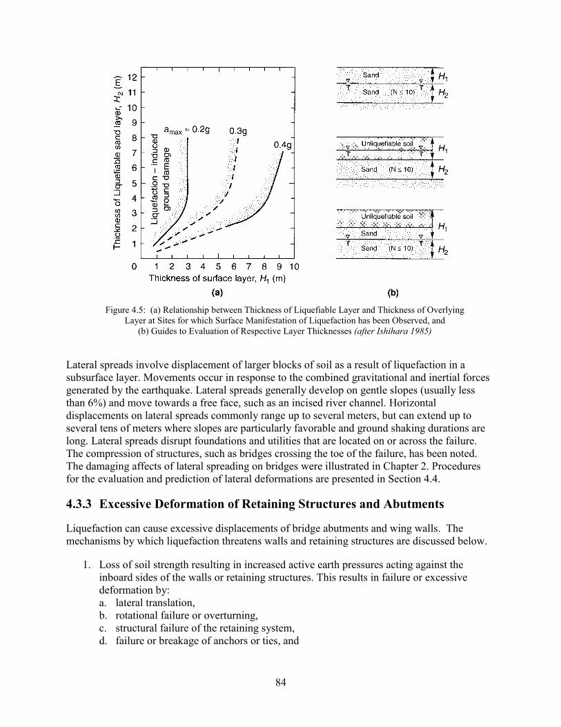
Figure 4.5: (a) Relationship between Thickness of Liquefiable Layer and Thickness of Overlying

Layer at Sites for which Surface Manifestation of Liquefaction has been Observed, and (b) Guides to Evaluation of Respective Layer Thicknesses (after Ishihara 1985)

Lateral spreads involve displacement of larger blocks of soil as a result of liquefaction in a subsurface layer. Movements occur in response to the combined gravitational and inertial forces generated by the earthquake. Lateral spreads generally develop on gentle slopes (usually less than 6%) and move towards a free face, such as an incised river channel. Horizontal displacements on lateral spreads commonly range up to several meters, but can extend up to several tens of meters where slopes are particularly favorable and ground shaking durations are long. Lateral spreads disrupt foundations and utilities that are located on or across the failure. The compression of structures, such as bridges crossing the toe of the failure, has been noted. The damaging affects of lateral spreading on bridges were illustrated in Chapter 2. Procedures for the evaluation and prediction of lateral deformations are presented in Section 4.4.

4.3.3 Excessive Deformation of Retaining Structures and Abutments

Liquefaction can cause excessive displacements of bridge abutments and wing walls. The mechanisms by which liquefaction threatens walls and retaining structures are discussed below.

1. Loss of soil strength resulting in increased active earth pressures acting against the inboard sides of the walls or retaining structures. This results in failure or excessive deformation by: a. lateral translation, b. rotational failure or overturning, c. structural failure of the retaining system, d. failure or breakage of anchors or ties, and

84

e. increased bearing loads at outboard toe of retaining system, promoting either rotational displacement or bearing failure.

2. Loss of soil strength resulting in decreased passive earth pressure or resistance that can be mobilized to prevent failure or displacement of the wall or retaining system. It is important to evaluate the hazards associated with potential loss of passive resistance at the outboard toe of the wall and earth-embedded anchors or tie-backs.

3. Overall stability and sliding due to loss of strength resulting in instability of a foundation soil unit beneath the wall or retaining system.

4.4 EMPIRICAL METHODS FOR ESTIMATING LATERAL SPREAD

DISPLACEMENT

In light of the complexity of modeling the dynamic behavior of liquefied soil, the most widely adopted methods for estimating lateral spread displacement are empirically-based procedures developed from case studies at sites around the world. For applications involving the preliminary screening of liquefaction hazards at bridge sites, a high degree of accuracy is not required; the empirical methods are adequate and can be conservatively applied. If lateral spreading hazards are indicated, then more sophisticated analyses may be warranted. These more rigorous analyses require substantial geotechnical data which may not be available for many projects. Because of the difficulty in precisely defining the requisite in situ soil properties at field sites, and the numerical uncertainty associated with FEM and FDM models, the results of advanced numerical modeling must be tempered with the results of the empirical methods.

The most straightforward empirical methods are based on extensive databases from case studies where measured displacements are correlated with site-specific topographic, geotechnical, and ground motion data. Hamada and others (1986) performed numerous pioneering studies of lateral spreading following earthquakes in Japan. They related lateral spread displacement to two simple parameters: the thickness of the liquefiable layer, and the slope angle. This method of evaluation began an intensive period of development of similar empirical methods (Youd and Perkins 1987; Bartlett and Youd 1995; Rauch and Martin 2000). Three simplified methods provide approximate estimates for lateral spread displacement; it is recommended that all three be used during the screening process for liquefaction hazards. These methods have the advantage of using standard field tests and soil classification properties for estimating lateral displacement. Final analysis and design will require more rigorous methods of estimating horizontal deformations and the impact of ground movements on bridge components.

4.4.1 The Liquefaction Severity Index

Youd and Perkins (1987) introduced the Liquefaction Severity Index (LSI) as a convenient method for estimating the maximum horizontal ground displacement expected at a given site. The derivation of the LSI was limited to lateral spreads that occurred on gently sloping ground or into river channels having widths greater than 10 m. The LSI database also was limited to highly to moderately liquefiable sites that were underlain by geologically young sediments having SPT N-values ranging from 2 to 10 blows/ft. For this specific geological-type setting, Youd and Perkins (1987) postulated that horizontal ground displacement is primarily a function of the amplitude and duration of strong ground motion. However, because strong motion records were

85

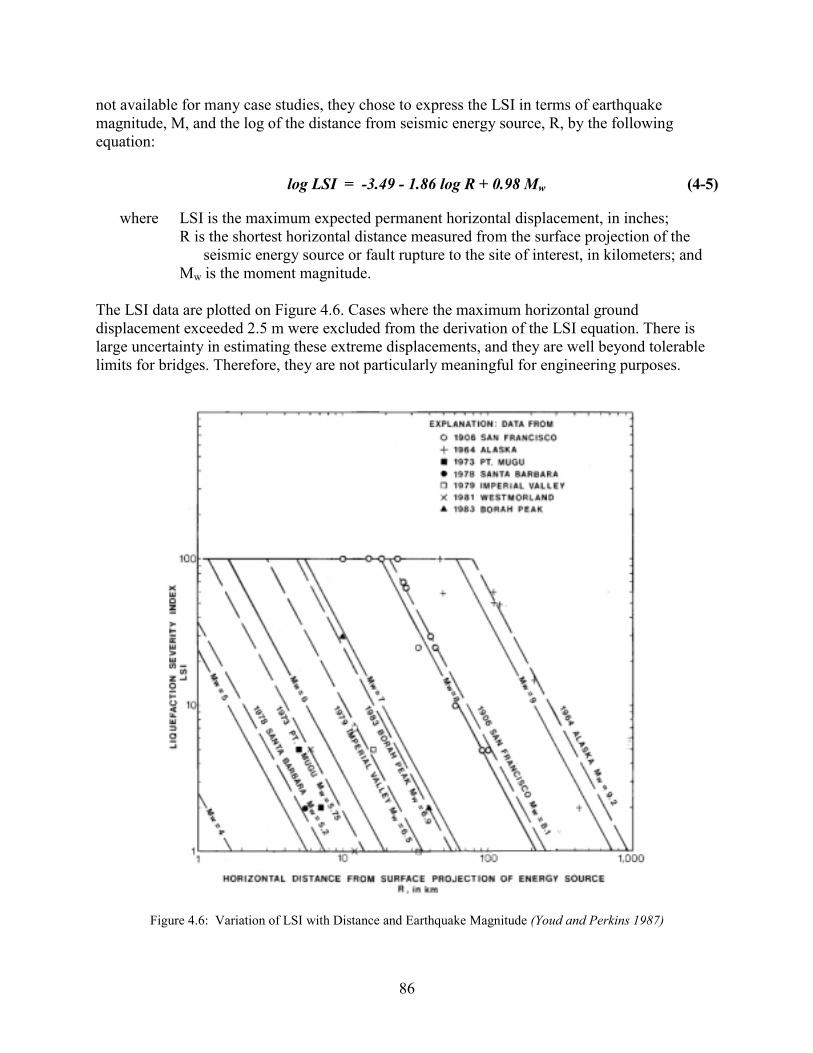
not available for many case studies, they chose to express the LSI in terms of earthquake magnitude, M, and the log of the distance from seismic energy source, R, by the following equation:

log LSI = -3.49 - 1.86 log R + 0.98 Mw (4-5)

where LSI is the maximum expected permanent horizontal displacement, in inches; R is the shortest horizontal distance measured from the surface projection of the

seismic energy source or fault rupture to the site of interest, in kilometers; and Mw is the moment magnitude.

The LSI data are plotted on Figure 4.6. Cases where the maximum horizontal ground displacement exceeded 2.5 m were excluded from the derivation of the LSI equation. There is large uncertainty in estimating these extreme displacements, and they are well beyond tolerable limits for bridges. Therefore, they are not particularly meaningful for engineering purposes.

Figure 4.6: Variation of LSI with Distance and Earthquake Magnitude (Youd and Perkins 1987)

86

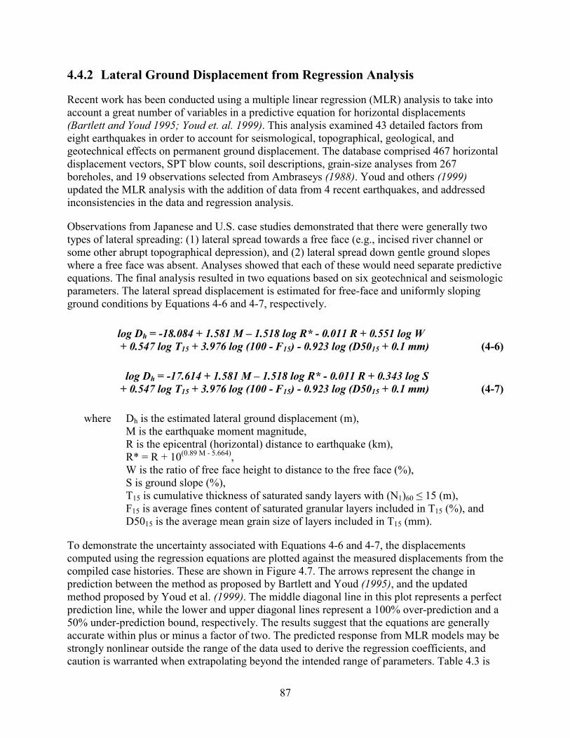
4.4.2 Lateral Ground Displacement from Regression Analysis

Recent work has been conducted using a multiple linear regression (MLR) analysis to take into account a great number of variables in a predictive equation for horizontal displacements (Bartlett and Youd 1995; Youd et. al. 1999). This analysis examined 43 detailed factors from eight earthquakes in order to account for seismological, topographical, geological, and geotechnical effects on permanent ground displacement. The database comprised 467 horizontal displacement vectors, SPT blow counts, soil descriptions, grain-size analyses from 267 boreholes, and 19 observations selected from Ambraseys (1988). Youd and others (1999) updated the MLR analysis with the addition of data from 4 recent earthquakes, and addressed inconsistencies in the data and regression analysis.

Observations from Japanese and U.S. case studies demonstrated that there were generally two types of lateral spreading: (1) lateral spread towards a free face (e.g., incised river channel or some other abrupt topographical depression), and (2) lateral spread down gentle ground slopes where a free face was absent. Analyses showed that each of these would need separate predictive equations. The final analysis resulted in two equations based on six geotechnical and seismologic parameters. The lateral spread displacement is estimated for free-face and uniformly sloping ground conditions by Equations 4-6 and 4-7, respectively.

log Dh = -18.084 + 1.581 M – 1.518 log R* - 0.011 R + 0.551 log W + 0.547 log T15 + 3.976 log (100 - F15) - 0.923 log (D5015 + 0.1 mm) (4-6)

log Dh = -17.614 + 1.581 M – 1.518 log R* - 0.011 R + 0.343 log S + 0.547 log T15 + 3.976 log (100 - F15) - 0.923 log (D5015 + 0.1 mm) (4-7)

where Dh is the estimated lateral ground displacement (m), M is the earthquake moment magnitude, R is the epicentral (horizontal) distance to earthquake (km), R* = R + 10(0.89 M - 5.664), W is the ratio of free face height to distance to the free face (%), S is ground slope (%), T15 is cumulative thickness of saturated sandy layers with (N1)60 ≤ 15 (m), F15 is average fines content of saturated granular layers included in T15 (%), and D5015 is the average mean grain size of layers included in T15 (mm).

To demonstrate the uncertainty associated with Equations 4-6 and 4-7, the displacements computed using the regression equations are plotted against the measured displacements from the compiled case histories. These are shown in Figure 4.7. The arrows represent the change in prediction between the method as proposed by Bartlett and Youd (1995), and the updated method proposed by Youd et al. (1999). The middle diagonal line in this plot represents a perfect prediction line, while the lower and upper diagonal lines represent a 100% over-prediction and a 50% under-prediction bound, respectively. The results suggest that the equations are generally accurate within plus or minus a factor of two. The predicted response from MLR models may be strongly nonlinear outside the range of the data used to derive the regression coefficients, and caution is warranted when extrapolating beyond the intended range of parameters. Table 4.3 is

87

provided to give the recommended ranges of input values for which the predicted displacements have been verified by comparison with the case-history data.

Figure 4.7: Comparison of Computed Lateral Spread Displacements with Observed Displacements

(Youd et. al., 1999)

Table 4.3: Ranges of Input Values for Independent Variables for Which Predicted Results are Verified by Case History Observations (Bartlett and Youd 1992)

INPUT FACTOR RANGE OF VALUES IN CASE HISTORY DATABASE Magnitude 6.0 < M < 8.0 Free-Face Ratio (%) 1.0 < W < 20.0 Ground Slope (%) 0.1 < S < 6.0 Thickness of Loose Layer (m) 0.3 < T15 < 12.0 Fines Content (%) 0.0 < F15 < 50.0 Mean Grain Size (mm) 0.1 < D5015 < 1.0

The results of the equation correspond to free-field conditions. Actual displacements near bridges may be less than predicted by the model, depending on the ability of the foundation to resist deformation. This reduction should not be anticipated unless supported by use of validated soil-structure interaction models. The range of verified slope angles is not in the range for most bridge embankments; therefore, the equation should be used to estimate movements away from the slope face which generally does not capture the area of most pronounced failures.

88

4.4.3 EPOLLS Model for Lateral Spread Displacement

The most recent model for estimating horizontal displacements is termed EPOLLS – Empirical Prediction of Liquefaction-Induced Lateral Spreading (Rauch and Martin 2000). The model was developed from a database of 71 historical lateral spreads using statistical regression techniques. The model can be used to estimate the average horizontal displacement given site-specific seismological, topographical, and geological parameters. The model has been formulated in three complementary parts: (1) the Regional-EPOLLS component, designed for seismic hazard surveys of geographic regions; (2) the Site-EPOLLS component, which gives improved predictions for site-specific studies; and (3) the Geotechnical-EPOLLS component, which uses additional data from subsurface explorations, thereby reducing uncertainty in the estimated lateral spread displacement. An overview of the EPOLLS model and the predictive equations used are shown in Figure 4.8. As with the method by Youd and others, this model should not be applied for scenarios that are significantly different from those cases used to develop the predictive equation.

4.5 ANALYTICAL METHODS FOR ESTIMATING LATERAL SPREAD DISPLACEMENT

The empirical methods for estimating lateral spread displacement are straightforward tools for preliminary hazard screening at bridge sites. Also, the empirical basis for the displacement estimates provides credibility to these methods. The methods are, however, limited in their application to the specific range of earthquakes, source-to-site distances, geological and geotechnical conditions, and topographies from the cases studies employed in the development of the predictive relationships. Most of the lateral spreads were evaluated at free-field sites. These conditions severely limit the application of the empirical methods for bridge sites with embankments and site-specific configurations. In these cases, the empirical approaches can be used only as approximate indicators of lateral spread hazard, and supplementary analysis procedures are required. Common methods of analysis include rigid body mechanics (i.e., the sliding-block methods) and numerical effective stress modeling.

4.5.1 Newmark Sliding Block Model

In most applications involving waterfront slopes and embankments, it is necessary to estimate the permanent slope deformations that may occur in response to the cyclic loading. Allowable deformation limits for slopes will reflect the sensitivity of adjacent structures, foundations and other facilities to these soil movements. Enhancements to traditional pseudostatic limit equilibrium methods of embankment analysis have been developed to estimate deformations for soils that do not lose appreciable strength during earthquake shaking (Makdisi and Seed 1978; Ambraseys and Menu 1988; Jibson 1993). These methods are not appropriate for modeling flow-type failures that can be associated with very loose saturated sands (N = 3-5 blows/ft).

89

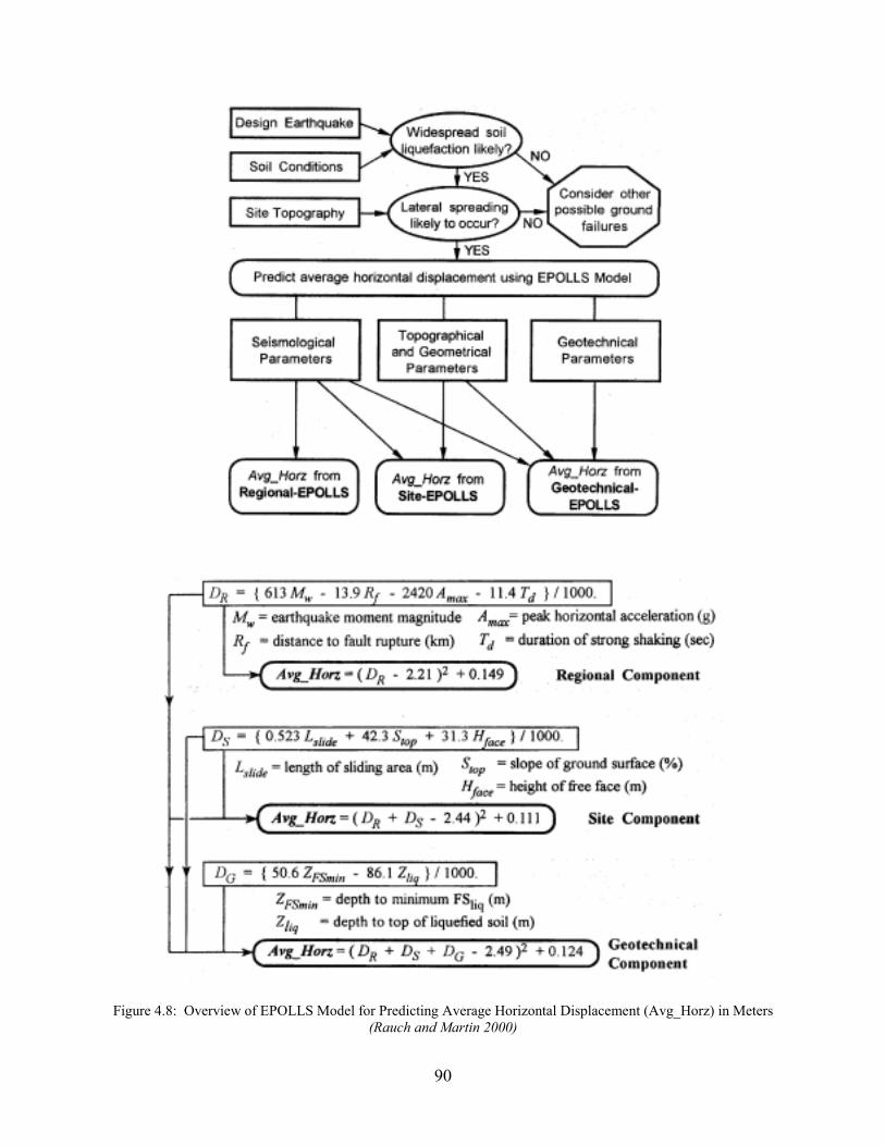
Figure 4.8: Overview of EPOLLS Model for Predicting Average Horizontal Displacement (Avg_Horz) in Meters (Rauch and Martin 2000)

90

Rigid body, sliding block analyses, which assume that the soil behaves as a rigid, perfectly plastic material, can be used to estimate limited earthquake-induced deformations. The technique, developed by Newmark (1965) and schematically illustrated in Figure 4.9, is based on simple limit equilibrium stability analysis for determining the critical, or yield, acceleration that is required to bring the factor of safety against sliding for a specified block of soil to unity. The yield acceleration is computed given the static factor of safety against sliding; it is expressed as

acrit = (FS – 1)g sin � (4-8)

where acrit is the critical acceleration in terms of g, the acceleration due to earth’s gravity;

FS is the static factor of safety; and is the angle (herein called the thrust angle) from the horizontal that the center

of mass of the potential landslide block first moves. �

Thus, determining the critical acceleration by this method requires knowing the static factor of safety and the thrust angle (Jibson 1993). The thrust angle is illustrated in Figure 4.10.

1) 2)

Figure 4.9: Elements of Sliding Block Analysis, (1) Hynes-Griffin and Franklin 1984; and 2) after Wilson and Keefer 1985)

91

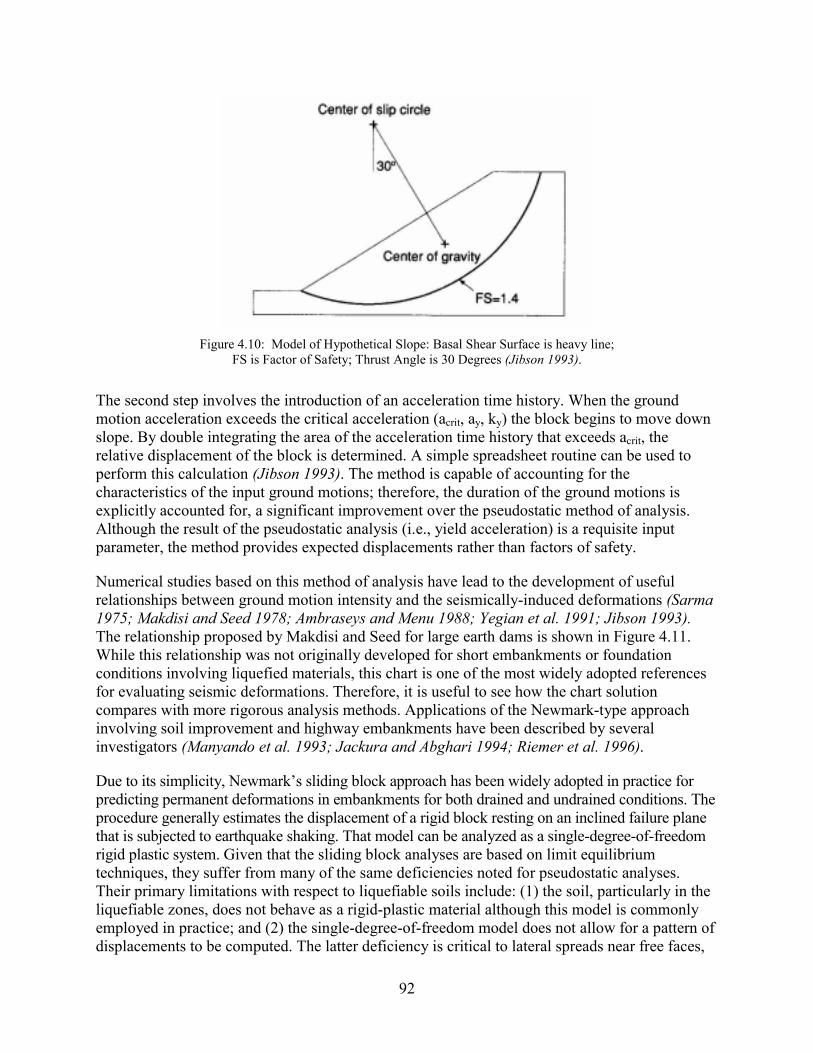
Figure 4.10: Model of Hypothetical Slope: Basal Shear Surface is heavy line;

FS is Factor of Safety; Thrust Angle is 30 Degrees (Jibson 1993).

The second step involves the introduction of an acceleration time history. When the ground motion acceleration exceeds the critical acceleration (acrit, ay, ky) the block begins to move down slope. By double integrating the area of the acceleration time history that exceeds acrit, the relative displacement of the block is determined. A simple spreadsheet routine can be used to perform this calculation (Jibson 1993). The method is capable of accounting for the characteristics of the input ground motions; therefore, the duration of the ground motions is explicitly accounted for, a significant improvement over the pseudostatic method of analysis. Although the result of the pseudostatic analysis (i.e., yield acceleration) is a requisite input parameter, the method provides expected displacements rather than factors of safety.

Numerical studies based on this method of analysis have lead to the development of useful relationships between ground motion intensity and the seismically-induced deformations (Sarma 1975; Makdisi and Seed 1978; Ambraseys and Menu 1988; Yegian et al. 1991; Jibson 1993). The relationship proposed by Makdisi and Seed for large earth dams is shown in Figure 4.11. While this relationship was not originally developed for short embankments or foundation conditions involving liquefied materials, this chart is one of the most widely adopted references for evaluating seismic deformations. Therefore, it is useful to see how the chart solution compares with more rigorous analysis methods. Applications of the Newmark-type approach involving soil improvement and highway embankments have been described by several investigators (Manyando et al. 1993; Jackura and Abghari 1994; Riemer et al. 1996).

Due to its simplicity, Newmark’s sliding block approach has been widely adopted in practice for predicting permanent deformations in embankments for both drained and undrained conditions. The procedure generally estimates the displacement of a rigid block resting on an inclined failure plane that is subjected to earthquake shaking. That model can be analyzed as a single-degree-of-freedom rigid plastic system. Given that the sliding block analyses are based on limit equilibrium techniques, they suffer from many of the same deficiencies noted for pseudostatic analyses. Their primary limitations with respect to liquefiable soils include: (1) the soil, particularly in the liquefiable zones, does not behave as a rigid-plastic material although this model is commonly employed in practice; and (2) the single-degree-of-freedom model does not allow for a pattern of displacements to be computed. The latter deficiency is critical to lateral spreads near free faces,

92

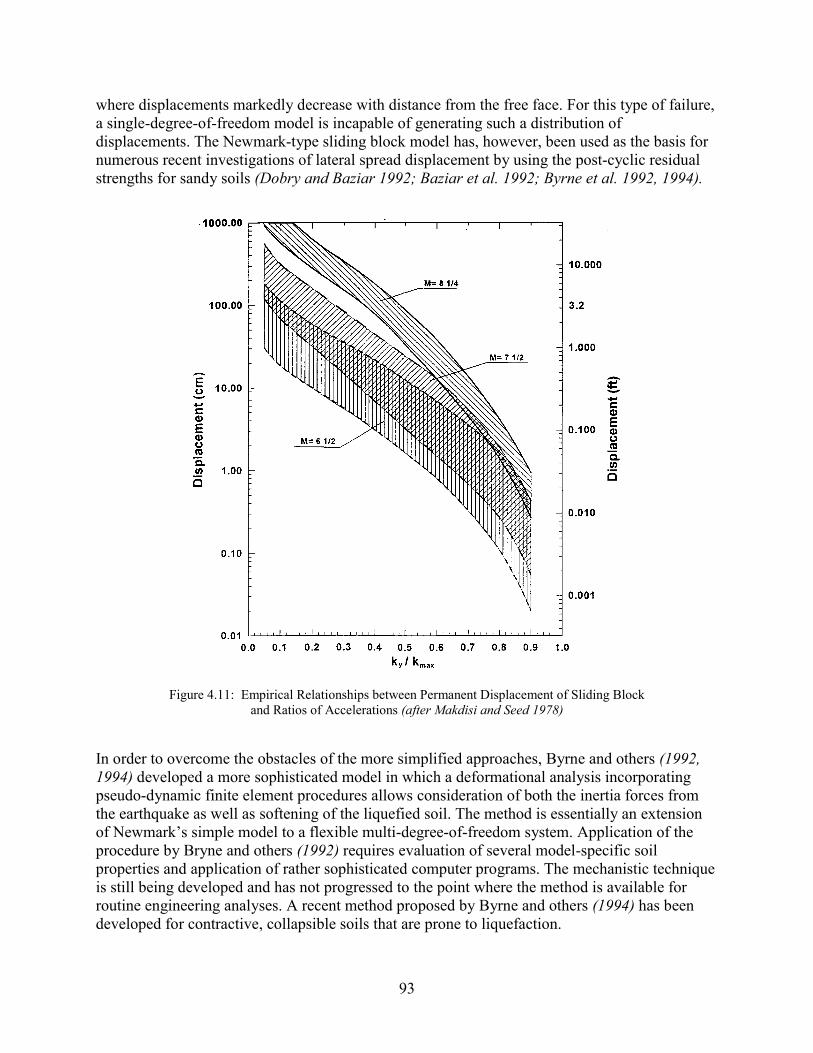
where displacements markedly decrease with distance from the free face. For this type of failure, a single-degree-of-freedom model is incapable of generating such a distribution of displacements. The Newmark-type sliding block model has, however, been used as the basis for numerous recent investigations of lateral spread displacement by using the post-cyclic residual strengths for sandy soils (Dobry and Baziar 1992; Baziar et al. 1992; Byrne et al. 1992, 1994).

Figur

In order to overc1994) developedpseudo-dynamicthe earthquake aof Newmark’s sprocedure by Brproperties and ais still being devroutine engineerdeveloped for co

e 4.11: Empirical Relationships between Permanent Displacement of Sliding Block and Ratios of Accelerations (after Makdisi and Seed 1978)

ome the obstacles of the more simplified approaches, Byrne and others (1992, a more sophisticated model in which a deformational analysis incorporating finite element procedures allows consideration of both the inertia forces from s well as softening of the liquefied soil. The method is essentially an extension imple model to a flexible multi-degree-of-freedom system. Application of the yne and others (1992) requires evaluation of several model-specific soil pplication of rather sophisticated computer programs. The mechanistic technique eloped and has not progressed to the point where the method is available for ing analyses. A recent method proposed by Byrne and others (1994) has been ntractive, collapsible soils that are prone to liquefaction.

93

4.5.2 Advanced Numerical Modeling of Slopes

In situations where the movement of a slope impacts adjacent structures such as abutments, spread footings, deep foundations, or buried lifelines, it is becoming more common to rely on numerical modeling methods to estimate the range of slope deformations which may be induced by design level ground motions (Finn 1990). The numerical models used for soil-structure interaction problems can be broadly classified based on the techniques that are used to account for the deformations of both the soil and the affected structural element. In many cases the movement of the soil is first computed, then the response of the structure to these deformations is determined. This type of analysis is termed uncoupled, in that the computed soil deformations are not affected by the existence of embedded structural components.

A common enhancement to this type of uncoupled analysis is the introduction of an iterative solution scheme that modifies the soil deformations based on the response of the structure so that compatible strains are computed. An example of this type of analysis is drag loading on piles due to lateral spreading. In an uncoupled analysis, the ground deformations would be estimated using either an empirical relationship (Bartlett and Youd 1995) or a sliding block type evaluation (Baziar et al. 1992; Byrne et al. 1994) as discussed in Section 4.4. Once the pattern of ground deformations has been established, a model such as LPILE (Reese and Wang 1994) can be used to determine the loads in the deformed piles. In addition, modifications can be made to the lateral soil resistance acting against piles (p-y curves) to account for the reduced stiffness and strength of the liquefied soil (O’Rourke et al. 1994). In the numerical models the lateral spread displacement is forced onto the p-y spring which loads the pile (i.e., drag loading).

In a coupled type of numerical analysis, the deformations of the soil and structural elements are solved concurrently. Two-dimensional numerical models such as FLUSH (Lysmer et al. 1975), FLAC (Itasca 1997), DYSAC2 (Muraleetharan et al. 1988), and LINOS (Bardet 1990) have been used to model the seismic performance of earth structures and pile-supported structures. The primary differences in these analyses include: (1) the numerical formulation employed (e.g., FEM, FDM, BEM), (2) the constitutive model used for the soils, and (3) the ability to model large, permanent deformations. Each of the methods listed have been useful in evaluating various aspects of dynamic soil-structure interaction.

Advanced numerical modeling techniques are recommended for soil-structure interaction applications, such as estimating permanent displacements of slopes and embankments with structural bridge elements. Key advantages of these models are: (1) complex embankment geometries can be evaluated, (2) sensitivity studies can be made to determine the influence of various parameters on the seismic stability of the structure, (3) dynamic soil behavior is more realistically reproduced, (4) coupled analyses allow factors such as excess pore pressure generation in contractive soils during ground shaking and the associated reduction of soil stiffness and strength to be used, and (5) soil-structure interaction and permanent deformations can be evaluated. Disadvantages of these techniques include: (1) the engineering time required to construct the numerical model can be extensive, (2) numerous soil parameters are often required, thereby increasing laboratory testing costs (the number of soil properties required is a function of the constitutive soil model employed in the model), and (3) very few of the available models have been validated with well documented case studies of the seismic performance of actual retaining structures; therefore, the level of uncertainty in the analysis is often unknown.

94

4.6 EVALUATION OF GROUND SETTLEMENTS FOLLOWING CYCLIC LOADING

As excess pore pressure generated by cyclic loading dissipates due to drainage, the soil consolidates, which results in ground settlement. Similarly, non-saturated cohesionless soils will contract during cyclic shearing resulting in surface settlements. The magnitude of the settlements will reflect the density of the soil, intensity of the ground motions, the factor of safety against liquefaction, and the thickness of the loose soil deposit. Field observations document post-earthquake settlements of soils adjacent to bridges of over 1 m (Hamada et al. 1995; Yasuda et al. 1996). These include flat sites in the absence of lateral spreading. Damage modes include pavement damage, uneven grades at the transition from soil to pile-supported approach structures, and abutment damage (Seed et al. 1990; Yasuda et al. 1996).

Several methods have been developed for estimating the magnitude of earthquake-induced settlements in sandy soils. The most widely adopted methods have been developed by Ishihara and Yoshimine (1992) and Tokimatsu and Seed (1987). The method proposed by Ishihara and Yoshimine has been produced in the form of a design chart relating volumetric strain in sandy soils to soil density and the factor of safety against liquefaction (FSL; Figure 4.12). This analysis requires that FSL be computed for the sandy deposit, or each sub-layer within the deposit. The methods outlined in Chapter 3 for estimating the triggering of liquefaction are used. The percent compression of each sub-layer can then be easily estimated by using Figure 4.12.

Although the procedure of Ishihara and Yoshimine was developed for saturated sandy soils it can be applied for unsaturated soils in an approximate manner. This assumes that volumetric behavior of a dry or partially saturated sand during drained cyclic loading is similar to the volumetric behavior of the soil following the application of undrained cyclic loading on a saturated specimen (i.e., post-loading consolidation due to the dissipation of excess pore pressure). In both scenarios the volumetric strain that is developed is a function of the initial void ratio of the soil, the effective confining stress prior to cyclic loading, and the intensity and duration of the cyclic loading.

As illustrated in Figure 4.12, in order to estimate the volumetric strain the factor of safety against liquefaction must be obtained. This calculation accounts for the influence of the four factors (e, �′c, CSR, MSF) previously listed on the estimated volumetric strain. Clearly, an unsaturated soil is not prone to liquefaction regardless of its density; therefore the concept of developing a factor of safety against liquefaction does not seem appropriate for this scenario. However, loose to medium dense sandy soils will experience volumetric strains during loading. A possible approach for applying the method to unsaturated soils is to first compute the FSL as if the soil were saturated, then enter the chart at the appropriate FSL and density. The results of this approximation should be tempered by calculations using the Tokimatsu and Seed method as follows. Because the Ishihara procedure was developed for clean sands, a correction is required for silty sands and silts. The (N1)60 values should be modified using correction factors for fines content (Youd and Idriss 1997) prior to using Figure 4.12. Also, the N1-values shown in Figure 4.12 correspond to typical Japanese equipment and procedures, and are thus representative of an SPT energy ratio of approximately ERm = 55%. The corrected and standardized SPT (N1)60 values used to develop estimates of FSL should be increased by about 10% when using Figure 4.12 to estimate the resulting volumetric compression.

95

Figure 4.12: Post Volumetric Shear Strain for Clean Sands (Ishihara and Yoshimine 1992)

The method for estimating the volumetric strain due to cyclic loading illustrated in Figure 4.12 is based on laboratory data from cyclic triaxial tests. In order to evaluate the suitability of the method for silts, the results of several laboratory investigations of Columbia River and Puget Sound soils (Dickenson and Brown 1997a, 1997b) have been superimposed on the basic chart.

Data corresponding to high quality field specimens of non-plastic silt are plotted in Figure 4.13(a) and data obtained on reconstituted specimens of non-plastic silt and silt of moderate plasticity (the PI of the Adair silt and Corvallis silt specimens is 10) are provided in Figure 4.13(b). The laboratory testing of these silts demonstrates that they exhibit post-cyclic loading volume change that is similar to that of loose- to medium-dense sand. It appears, based on this very limited data, that the method of Ishihara and Yoshimine (1992) can be used to estimate settlements due to seismic loading of non-plastic to low-plasticity silt.

The procedure for estimating of soil densification and related settlements developed by Tokimatsu and Seed (1987) can be used for saturated or nearly saturated soils, and for non-saturated soils. The Tokimatsu and Seed method proceeds in steps that are very similar to those prescribed by Ishihara and Yoshimine (1992). The liquefaction susceptibility is again performed for each loose- to medium-dense cohesionless soil layer, using simplified procedures described in Chapter 3. For each soil layer or sub-layer, a representative estimate of (N1)60 and CSReq are required. Given this information, the volumetric strain can be estimated from the chart of CSReq (or τav / σo

′ as indicated in the figure) versus (N1)60, as presented in Figure 4.14.

96

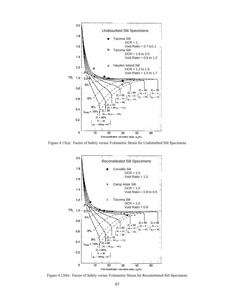
Undisturbed Silt Specimens

Tacoma SiltOCR = 1,Void Ratio = 0.7 to1.1

Tacoma SiltOCR = 1.8 to 2.0Void Ratio = 0.9 to 1.2

Hayden Island SiltOCR = 1.2 to 1.9Void Ratio = 1.0 to 1.7

Figure 4.13(a): Factor of Safety versus Volumetric Strain for Undisturbed Silt Specimens

Reconstituted Silt Specimens

Corvallis SiltOCR = 1.0Void Ratio = 1.0

Camp Adair SiltOCR = 1.0Void Ratio = 0.8 to 0.9

Tacoma SiltOCR = 1.0Void Ratio = 0.8

Figure 4.13(b): Factor of Safety versus Volumetric Strain for Reconstituted Silt Specimens

97

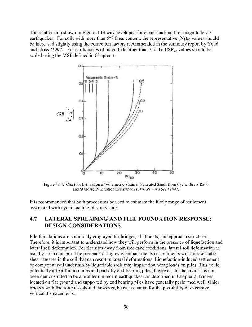
The relationship shown in Figure 4.14 was developed for clean sands and for magnitude 7.5 earthquakes. For soils with more than 5% fines content, the representative (N1)60 values should be increased slightly using the correction factors recommended in the summary report by Youd and Idriss (1997). For earthquakes of magnitude other than 7.5, the CSReq values should be scaled using the MSF defined in Chapter 3.

��

�

�

��

�

�

'oσCSR av�

Figure 4.14: Chart an

It is recommended that associated with cyclic l

4.7 LATERAL SDESIGN CO

Pile foundations are comTherefore, it is importalateral soil deformationusually not a concern. Tshear stresses in the soiof competent soil underpotentially affect frictiobeen demonstrated to blocated on flat ground abridges with friction pilvertical displacements.

for Estimation of Volumetric Strain in Saturated Sands from Cyclic Stress Ratio d Standard Penetration Resistance (Tokimatsu and Seed 1987)

both procedures be used to estimate the likely range of settlement oading of sandy soils.

PREADING AND PILE FOUNDATION RESPONSE: NSIDERATIONS

monly employed for bridges, abutments, and approach structures. nt to understand how they will perform in the presence of liquefaction and . For flat sites away from free-face conditions, lateral soil deformation is he presence of highway embankments or abutments will impose static

l that can result in lateral deformations. Liquefaction-induced settlement lain by liquefiable soils may impart downdrag loads on piles. This could n piles and partially end-bearing piles; however, this behavior has not e a problem in recent earthquakes. As described in Chapter 2, bridges nd supported by end bearing piles have generally performed well. Older es should, however, be re-evaluated for the possibility of excessive

98

Lateral ground flow and its effect on foundation piles has been the focus of recent investigations. Generally, research on this topic has followed three lines of investigation:

1. Empirical evaluation based on case studies (Fujii et al. 1998; Tokimatsu et al. 1998). 2. Numerical modeling of pile response (Miura and O’Rourke 1991; Meyerson et al. 1992;

O’Rourke et al. 1994; Ishihara and Cubrinovski 1998a, 1998b; Wang and Reese 1998). 3. Centrifuge modeling (Abdoun et al. 1996; Horikoshi et al. 1997; Boulanger et al. 1999).

As mentioned in Chapter 1, many of these studies were undertaken in response to the observations of excavated piles damaged during the 1964 Niigata Earthquake. The results of these analytical studies have provided valuable information regarding the interaction between piles and liquefied soil including the failure modes of piles subjected to these lateral movements.

4.7.1 Pile Failure Modes

Several distinctive failure modes have been identified for piles subjected to liquefaction-induced lateral ground movements. In the first mode, the pile may buckle due to the lack of sufficient lateral support resulting from the reduced stiffness of the liquefied soil in combination with the increased lateral deflection imposed on the pile. In the second, the pile reaches its bending capacity due to lateral pile deflections caused by the horizontal soil displacement. In this case, a plastic hinge develops. Figure 4.15 illustrates these possible failure mechanisms; buckling and plastic hinge formations are shown in Figures 4.15(a) and 4.15(b), respectively. The depth to water in the diagrams indicates the possible extent of an upper non-liquefied layer. The dual groundwater tables in Figure 4.15 (b) and (c) represent fluctuations in the location of the water level due to seasonal or tidal influences. The thickness of the liquefiable layer will be affected by these variations in the groundwater table.

Soil Displacement

Liquefied soil

Non-liquefied soil/Rock

Figure 4.15: Potential Modes of Pile Failure Due to Lateral Loading by Liquefied Soil (Meyerson et al. 1992)

Whether the pile’s bending capacity is first reached in the vicinity of the upper or lower interface depends on the amount of lateral restraint offered by the nonliquefied soil. In general, hinge formation will tend to occur at the lower interface, since the higher confining effective stress at greater depth results in larger lateral resistance than at shallower depth (O’Rourke et al. 1994).

99

A third type of failure is shown in Figure 4.15(c). It involves excessive body rotation of the pile, which is characteristic of larger diameter piles and piers. This response to lateral soil movement is primarily due to insufficient restraint at the bottom of the pile because of inadequate embedment length or a low resistance of the foundation material against lateral deformation.

Two additional modes of loading observed following recent earthquakes include lateral loads due to soil flow around the piles, and concentration of load on piles at the interface of weak and dense soil layers at depth. The former mode is characterized by the flow of liquefied soil around the pile and is usually associated with stiff foundations, such as large diameter piles, piers, and groups of closely spaced piles. Under these conditions, a relatively stiff pile will flex until the soil has mobilized its full resistance against the pile. Additional soil movement occurs as a flow relative to the pile. The latter mode resulted in extensive damage to piles during the Kobe Earthquake (Iai 1998). Moment concentration at the interface between a loose- to medium-dense sand and an underlying dense sand and gravel deposit resulted in the formation of plastic hinges at depths greater than those normally associated with the “depth of fixity” used in analyses of pile response to lateral loading. This demonstrates a significant limitation in current analysis and design of piles for dynamic conditions. The potential for load concentration at layer interfaces should be evaluated for sites exhibiting pronounced variations of soil stiffness (due to soil liquefaction or existence of weak soils such as marine clays, deltaic-estuarine silt deposits, etc.).

The seismic performance of pile foundations in liquefiable soils remains a topic of intensive research. The performance of deep foundations is a complex function of the following site-specific parameters:

1. intensity and duration of the strong ground motions; 2. extent of the liquefiable soil deposit; 3. site topography; 4. pile type(s), group size and configuration relative to the direction of soil movement, pile

spacing; 5. pile restraint (i.e., fixed-head, free-head condition); and 6. pile design and fabrication, which dictates allowable curvature and moments.

In addition, the following topics are poorly understood: (1) possible slope reinforcement provided by piles in embankments and reduction in seismically-induced deformations, (2) performance of piles in improved ground, and (3) seismic performance of batter piles in competent ground. It is currently recommended that numerical dynamic, effective stress soil-structure interaction analyses be performed for evaluating the seismic performance of embankments and foundations of important bridges (categorized on the basis of the Liquefaction Mitigation Policy). For other bridges, it is recommended that the conventional liquefaction hazard analyses described in this report be used to estimate seismically-induced deformations of embankments and foundation soils. If excessive ground deformations are indicated, soil improvement options should be implemented and the optimal volume of ground treatment identified, given the tolerable displacement limits and ground motion parameters. When using standard limit equilibrium methods, the potential embankment or slope reinforcement provided by piles should not be relied upon. Instead, it is recommended that the ground deformations be evaluated in the absence of piles, and the piles are assumed to move with the surrounding soil.

100

5.0 MITIGATION OF LIQUEFACTION HAZARDS

5.1 INTRODUCTION

If a seismic hazard assessment demonstrates that liquefaction is likely adjacent to a bridge and approach structures, and geotechnical/structural limit states may be exceeded, mitigation strategies should be evaluated. Generally, seismic strengthening can be achieved by soil improvement and/or structural enhancement. Only soil improvement techniques are addressed here. The goal of remedial soil improvement is to limit soil displacements and settlements to acceptable levels.

Guidance on the seismic performance of bridge foundations in liquefiable soils and tolerable movement criteria for highway bridges can be found in several Federal Highway Administration reports (FHWA 1985; Lam and Martin 1986a, 1986b, 1986c) and professional papers (Youd 1993; Zelinski et al. 1995). This chapter summarizes a review of the literature on soil improvement for mitigating seismic hazards. It provides an introduction to ground treatment methods utilized to mitigate seismic hazards at bridge sites and contains references pertaining to the analysis, design, and seismic performance of ground treatment applications.

Remedial strategies for improving the stability of slopes and embankments have been well developed for both onshore and submarine slopes. Common techniques for stabilizing slopes include: (1) modifying the geometry of the slope; (2) utilization of berms; (3) soil replacement (key trenches with engineered fill); (4) soil improvement; and (5) structural techniques such as the installation of piles adjacent to the toe of the slope. Constraints imposed by existing structures will often dictate which methods, or combination of methods, should be used (Koelling and Dickenson 1998). The report, Guide to Remedial Measures for Liquefaction Mitigation at Existing Highway Bridge Sites by Cooke and Mitchell (1999) provides thorough and practice-oriented guidelines for the application of soil improvement. This reference, along with the reports Screening Guide for Rapid Assessment of Liquefaction Hazard at Highway Bridge Sites (Youd 1998) and Handbook on Liquefaction Remediation of Reclaimed Land (PHRI 1997) are highly recommended.

5.2 TECHNIQUES FOR MITIGATING LIQUEFACTION HAZARDS

Remediation objectives include increasing the soil’s liquefaction resistance through densification, increasing its strength, and/or improving its drainage. Table 5.1 presents the most common remediation measures. The use of these measures has limited the occurrence of liquefaction during recent earthquakes.

101

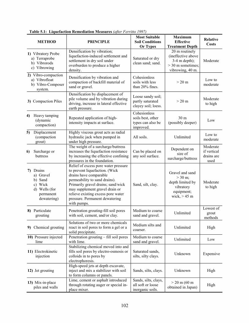
Table 5.1: Liquefaction Remediation Measures (after Ferritto 1997)

METHOD PRINCIPLE Most Suitable

Soil Conditions Or Types

Maximum Effective

Treatment Depth

Relative Costs

1) Vibratory Probe a) Terraprobe b) Vibrorods c) Vibrowing

Densification by vibration; liquefaction-induced settlement and settlement in dry soil under overburden to produce a higher density.

Saturated or dry clean sand; sand.

20 m routinely (ineffective above

3-4 m depth); > 30 m sometimes; vibrowing, 40 m.

Moderate

2) Vibro-compaction a) Vibrofloat b) Vibro-Composer

system.

Densification by vibration and compaction of backfill material of sand or gravel.

Cohesionless soils with less than 20% fines.

> 20 m Low to moderate

3) Compaction Piles

Densification by displacement of pile volume and by vibration during driving, increase in lateral effective earth pressure.

Loose sandy soil; partly saturated clayey soil; loess.

> 20 m Moderate to high

4) Heavy tamping (dynamic compaction)

Repeated application of high-intensity impacts at surface.

Cohesionless soils best, other types can also be improved.

30 m (possibly deeper) Low

5) Displacement (compaction grout)

Highly viscous grout acts as radial hydraulic jack when pumped in under high pressure.

All soils. Unlimited Low to moderate

6) Surcharge or buttress

The weight of a surcharge/buttress increases the liquefaction resistance by increasing the effective confining pressures in the foundation.

Can be placed on any soil surface.

Dependent on size of

surcharge/buttress

Moderate if vertical drains are

used

7) Drains a) Gravel b) Sand c) Wick d) Wells (for

permanent dewatering)

Relief of excess pore water pressure to prevent liquefaction. (Wick drains have comparable permeability to sand drains). Primarily gravel drains; sand/wick may supplement gravel drain or relieve existing excess pore water pressure. Permanent dewatering with pumps.

Sand, silt, clay.

Gravel and sand > 30 m;

depth limited by vibratory

equipment; wick, > 45 m

Moderate to high

8) Particulate grouting

Penetration grouting-fill soil pores with soil, cement, and/or clay.

Medium to coarse sand and gravel. Unlimited

Lowest of grout

methods

9) Chemical grouting Solutions of two or more chemicals react in soil pores to form a gel or a solid precipitate.

Medium silts and coarser. Unlimited High

10) Pressure injected lime

Penetration grouting – fill soil pores with lime.

Medium to coarse sand and gravel. Unlimited Low

11) Electrokinetic injection

Stabilizing chemical moved into and fills soil pores by electro-osmosis or colloids in to pores by electrophoresis.

Saturated sands, silts, silty clays. Unknown Expensive

12) Jet grouting High-speed jets at depth excavate, inject and mix a stabilizer with soil to form columns or panels.

Sands, silts, clays. Unknown High

13) Mix-in-place piles and walls

Lime, cement or asphalt introduced through rotating auger or special in-place mixer.

Sands, silts, clays, all soft or loose inorganic soils.

> 20 m (60 m obtained in Japan) High

102

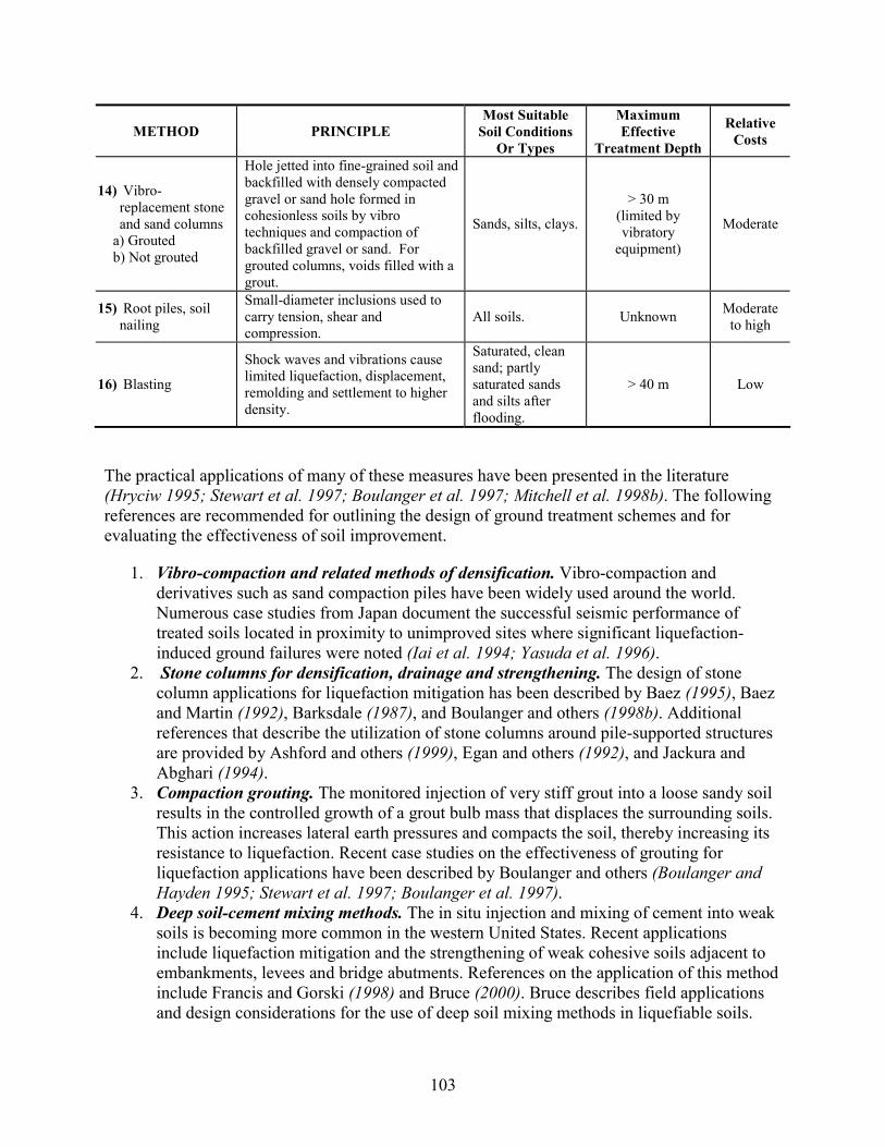
METHOD PRINCIPLE Most Suitable

Soil Conditions Or Types

Maximum Effective

Treatment Depth

Relative Costs

14) Vibro-replacement stone and sand columns

a) Grouted b) Not grouted

Hole jetted into fine-grained soil and backfilled with densely compacted gravel or sand hole formed in cohesionless soils by vibro techniques and compaction of backfilled gravel or sand. For grouted columns, voids filled with a grout.

Sands, silts, clays.

> 30 m (limited by vibratory

equipment)

Moderate

15) Root piles, soil nailing

Small-diameter inclusions used to carry tension, shear and compression.

All soils. Unknown Moderate to high

16) Blasting

Shock waves and vibrations cause limited liquefaction, displacement, remolding and settlement to higher density.

Saturated, clean sand; partly saturated sands and silts after flooding.

> 40 m Low

The practical applications of many of these measures have been presented in the literature (Hryciw 1995; Stewart et al. 1997; Boulanger et al. 1997; Mitchell et al. 1998b). The following references are recommended for outlining the design of ground treatment schemes and for evaluating the effectiveness of soil improvement.

1. Vibro-compaction and related methods of densification. Vibro-compaction and derivatives such as sand compaction piles have been widely used around the world. Numerous case studies from Japan document the successful seismic performance of treated soils located in proximity to unimproved sites where significant liquefaction-induced ground failures were noted (Iai et al. 1994; Yasuda et al. 1996).

2. Stone columns for densification, drainage and strengthening. The design of stone column applications for liquefaction mitigation has been described by Baez (1995), Baez and Martin (1992), Barksdale (1987), and Boulanger and others (1998b). Additional references that describe the utilization of stone columns around pile-supported structures are provided by Ashford and others (1999), Egan and others (1992), and Jackura and Abghari (1994).

3. Compaction grouting. The monitored injection of very stiff grout into a loose sandy soil results in the controlled growth of a grout bulb mass that displaces the surrounding soils. This action increases lateral earth pressures and compacts the soil, thereby increasing its resistance to liquefaction. Recent case studies on the effectiveness of grouting for liquefaction applications have been described by Boulanger and others (Boulanger and Hayden 1995; Stewart et al. 1997; Boulanger et al. 1997).

4. Deep soil-cement mixing methods. The in situ injection and mixing of cement into weak soils is becoming more common in the western United States. Recent applications include liquefaction mitigation and the strengthening of weak cohesive soils adjacent to embankments, levees and bridge abutments. References on the application of this method include Francis and Gorski (1998) and Bruce (2000). Bruce describes field applications and design considerations for the use of deep soil mixing methods in liquefiable soils.

103

5.3 DESIGN OF SOIL MITIGATION

The design of soil mitigation strategies involves investigating the cost/benefit ratio, the seismic performance, and the effect of the mitigation technique(s) on adjacent structures. The mitigation methods listed in Table 5.1 can be generally categorized in terms of their affect on the soil: compaction, drainage, or cementation. The design for each of these remediation categories is briefly discussed below. A more in-depth discussion on the design of soil mitigation strategies and procedures may be found in the reference Handbook on Liquefaction Remediation of Reclaimed Land (PHRI 1997).

Compaction remediation methods densify the soil with vibration or impact (examples include methods 1, 2, 3, 4 and 14 from Table 5.1). Compaction methods are more suitable for use in saturated, cohesionless soils with a limited percentage of fines. They cause noise and vibration during installation, and also increase horizontal earth pressures against adjacent structures. This increase in pressure is the major disadvantage of using compaction methods in close proximity to retaining walls. The major advantage of compaction methods is the relatively low cost/benefit ratio. The necessary degree of compaction can be evaluated using penetration resistances that have been back-calculated from an acceptable factor of safety against liquefaction (Chapter 3).

Drainage remediation methods enhance the rate of excess pore pressure dissipation. The most common methods use gravel, sand or wick drains. Drains are suitable for use in sands, silts or clays. One of the greatest advantages of drains is that they induce relatively small horizontal earth pressures during installation. Therefore, they are suitable for use adjacent to sensitive structures. In the design of drains, it is necessary to select a suitable drain material that has a coefficient of permeability substantially larger than the in situ soils.

Cementation remediation methods increase soil strength by adding a cementatious material (i.e. cement, grout, lime, chemicals, asphalt). Cementation techniques (methods 5, 8, 9, 10, 12, and 14 from Table 5.1) can be used with any type of soil. They are advantageous because the installation methods are relatively quiet and induce relatively small vibrations as compared to compaction methods. The induced horizontal earth pressures are smaller than with compaction methods, and are larger than with drainage methods. Their disadvantage is the relatively high cost/benefit ratio as compared to compaction and drainage methods.

The relative performance of the specific improvement method also is of concern in the design of a mitigation program. Experience has demonstrated that compaction and cementation techniques reduce the liquefaction susceptibility of soils to a larger extent than drainage methods alone.

The influence of ground treatment on existing structures is a primary design consideration. The construction methods may lead to increased horizontal earth pressures, which can result in deformations of embankments, walls and pile foundations. Mitigation methods also may induce excess pore pressures and vibration, which will affect sloping embankments and retaining structures. Therefore, a mitigation strategy design may include the combination of two or more improvement techniques in order to take advantage of robust treatment methods in free field areas and less disturbing methods close to existing structures. In general, compaction techniques have the largest impact on adjacent structures, followed by controlled cementation techniques, and then drainage methods, which generally are the least disruptive.

104

5.4 DESIGN FOR THE AREA OF SOIL MITIGATION

Specifying the extent of ground treatment adjacent to a bridge is not often a straightforward process. The costs associated with soil improvement must be balanced against the anticipated reduction in ground deformations during the design-level earthquake(s). An iterative approach is commonly employed where the seismic performance of a site is evaluated as a function of the volume of ground treatment utilized. The acceptable seismic performance of a foundation or approach fill will reflect the anticipated earthquake-induced displacements, the sensitivity of the structural elements impacted by the soil deformations, and the importance of the structure. At some point it becomes clear that additional soil improvement is not justified from a performance and cost perspective. In light of the site-specific nature of the problem, very few design manuals or guidelines for establishing the extent of soil improvement adjacent to bridges are available. From a practical perspective, this situation is further complicated because deformation-based analyses are the most appropriate procedures for evaluating the effectiveness of soil improvement.

The Japan PHRI and the Japanese Geotechnical Society have produced design guidelines (PHRI 1997; JGS 1998) for specifying the extent of soil improvement adjacent to various structures. The recommendations contained in these references are largely based on the results of physical and numerical modeling of gravity retaining walls. These modeling efforts have demonstrated that the migration of excess pore pressures generated in the unimproved liquefiable soils adjacent to the treated soil can lead to large strain development in the improved soil, due to reduced shear resistance. It has been shown that ru ratios greater than 0.5 should be considered problematic in the treated soils (note that this ru is due to dissipation of excess pore pressures from the unimproved soil). The influence of excess pore pressure migration from zones of liquefied soil to non-liquefied soils has also been reported by Mitchell and others (1998).

The lateral dimension of the improved soil that is affected by the excess pore pressures from the unimproved soil is approximately equal to half the thickness of the liquefied deposit. For the case of bearing capacity of footings or mat foundations, the area of soil improvement must therefore be extended laterally from the proposed structure by an amount equal to half the thickness of the layer that is predicted to liquefy.

Guidelines for applications involving retaining walls or piles are modified to ensure the zones of soil that that are subjected to static stresses (e.g., zones bounded by the active or passive failure surfaces) and the dynamic components of loading are not further impacted by the reduction in shear strength due to the reduction in effective stress. Examples incorporating soil improvement adjacent to gravity retaining walls and pile foundations are shown in Figures 5.1 and 5.2. The dimension CF, (or DE) is determined by first establishing the active failure surface for dynamic conditions. From the point where the active failure surface reaches the ground surface (a width equal to AE or BF) the zone of soil requiring treatment is increased by a distance equal to half the thickness of the liquefiable soil deposit. This ensures that the soil in the active failure wedge is not affected by the excess pore pressure developed in the unimproved soil.

Pressures from the liquefied part of the ground contribute to the stability of the structures as shown in Figure 5.2. The pressures amount to the static pressure equivalent determined using a lateral earth pressure coefficient of 1.0 minus the dynamic earth pressure (JGS 1998). The JGS

105

soil improvement guidelines state that for simplicity in the stability analysis, these procedures can be applied to the surface CD in Figure 5.2.

Figure 5.1: Improvement Area for Gravity Retaining Structures (PHRI 1997; JGS 1998)

Figure 5.2: Improvement Area for Pile Foundation and Underground Structure (PHRI 1997; JGS 1998)

106

For the pile foundation shown in Figure 5.2, the depth 1/� is the depth of fixity commonly used in structural models of pile foundations. This measure is a function of geotechnical and structural design parameters (soil stiffness and strength, pile type, pile stiffness, pile diameter). For preliminary analysis the depth of fixity can be assumed to be equal to 5 times the pile diameter. This value should be refined as project-specific geotechnical and structural data are obtained.

The line HD is established by sketching the passive failure surface from to outside row of piles at depth H = 1/�, up to the ground surface. The angle of this plane from the horizontal is (45 - �/2), where � is the effective angle of internal friction of the soil. Once point D has been established, the width of the improved soil that will be affected by the migration of pore pressures due to liquefaction in the unimproved soil is established as previously outlined (this provides point A at the ground surface). The plane II′ represents the intersection of the passive failure surface with the plane inclined at 30� from the vertical, as illustrated in Figure 5.2. As outlined in the JGS guidelines, for stability analyses of pile foundations the lateral earth pressures can be applied at the plane II′.

There is uncertainty in evaluating the relative effectiveness of ground treatment strategies for limiting lateral deformations because a limited amount of research has been performed to evaluate seismically-induced lateral deformations of improved soil sites. Several recent investigations have employed physical modeling (i.e., centrifuge and shaking tables) to evaluate the seismic performance of embankments with and without soil improvement (Adalier et al. 1998). Adalier utilized centrifuge modeling to evaluate the effectiveness of ground treatment and stabilization measures for mitigating deformations of embankments. Model embankments of clayey sand underlain by liquefiable sand were tested for cases involving: (1) no improvement of the foundation soil, (2) densification of the foundation soils, (3) solidification of the foundation soil, (4) the application of gravel berms adjacent to the embankment, and (5) the utilization of sheetpile walls along the toe of the embankment (Figure 5.3).

Figure 5.3: Models of Embankments in Clayey Sand Underlain by Liquefiable Sands (Adalier et al. 1998)

107

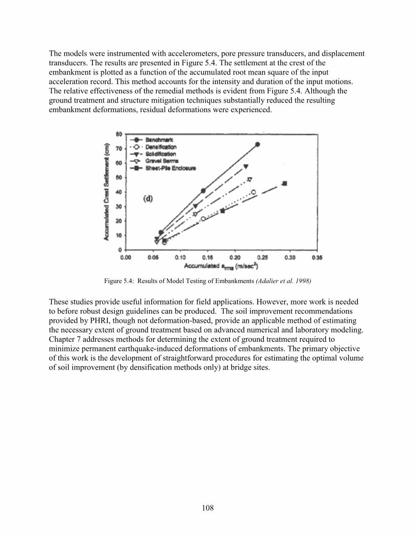
The models were instrumented with accelerometers, pore pressure transducers, and displacement transducers. The results are presented in Figure 5.4. The settlement at the crest of the embankment is plotted as a function of the accumulated root mean square of the input acceleration record. This method accounts for the intensity and duration of the input motions. The relative effectiveness of the remedial methods is evident from Figure 5.4. Although the ground treatment and structure mitigation techniques substantially reduced the resulting embankment deformations, residual deformations were experienced.

Figure 5.4: Results of Model Testing of Embankments (Adalier et al. 1998)

These studies provide useful information for field applications. However, more work is needed to before robust design guidelines can be produced. The soil improvement recommendations provided by PHRI, though not deformation-based, provide an applicable method of estimating the necessary extent of ground treatment based on advanced numerical and laboratory modeling. Chapter 7 addresses methods for determining the extent of ground treatment required to minimize permanent earthquake-induced deformations of embankments. The primary objective of this work is the development of straightforward procedures for estimating the optimal volume of soil improvement (by densification methods only) at bridge sites.

108

6.0 NUMERICAL MODELING

The database of well characterized and instrumented case studies on the seismic performance of bridge abutments on sloping embankments is very limited. Such cases require pre- and post-earthquake geotechnical and survey data, recorded earthquake motions in vicinity of the site (or a reasonable estimate of the ground motions from a site response investigation), structural “as-built” drawings of the bridge and abutments affected by the ground motions, and the extraction of piles to inspect for possible subsurface damage. To supplement the case study data, a numerical modeling study was conducted. A numerical model is advantageous because numerous scenarios can be analyzed, and various design parameters can easily be adjusted to determine their influence on an embankment’s seismic performance. The major concern with applying a model to soil-structure interaction problems is the numerical uncertainty. This concern is limited in this study because a series of validation studies were performed using the available case study data on the seismic performance of various earth and retaining structures at sites where liquefaction was observed.

The numerical modeling was accomplished utilizing a commercial finite difference computer program entitled Fast Lagrangian Analysis of Continua (FLAC) version 3.34 (Itasca Consulting Group 1997). The FLAC model is a non-linear, two-dimensional finite difference program capable of modeling both static and dynamic situations. Elements or zones represent the materials (soil and structural), with all the elements and zones constituting the grid (mesh). The FLAC model utilizes a time-marching scheme, where during each timestep, the following procedures take place (Figure 6.1): (1) nodal velocities and displacements are calculated from stresses and forces using the equations of motion, then (2) the basic explicit calculation sequence uses the velocities to computes strain rates, which are derived from the nodal velocities, which are used to update the stresses used in the following time step are computed from the strain rates. .These two procedures are then repeated until the computed unbalanced forces within the mesh are within a user-specified limit.

Equilibrium Equation(Equation of Motion)

Stress/Strain Relationship(Constitutive Model)

new velocitiesand

displacements

newstresses or

forces

Figure 6.1: Basic Explicit Calculation Cycle

109

The model uses an explicit method, where the calculation timestep is very short compared with the time necessary for information (acceleration, velocity, displacement) to physically pass from one element to another. It also utilizes a Lagrangian formulation, where the incremental displacements are added to the coordinates at each timestep so that the grid moves and deforms with the material it represents.

There are several advantages and disadvantages in using FLAC as compared to implicit finite element programs (Table 6.1). Because of the explicit Lagrangian methodology and the explicit use of the equations of motion, FLAC is advantageous in modeling non-linear, large strain, physically unstable situations (Itasca Consulting Group 1997).

Table 6.1: Comparison of FLAC and Finite Element Numerical Programs FLAC (Explicit) Finite Element (Implicit)

Timestep must be smaller than a critical value for stability.

Timestep can be arbitrarily large, with unconditionally stable schemes.

Small amount of computation effort per timestep. Large amount of computational effort per timestep. No significant numerical damping introduced for dynamic solution.

Numerical damping dependent on timestep present with unconditionally stable schemes.

No iterations necessary to follow nonlinear constitutive law.

Iterative procedure necessary to follow nonlinear constitutive law.

Provided that the timestep criterion is always satisfied, nonlinear laws are always followed in a valid physical way.

Always necessary to demonstrate that the above mentioned procedure is a) stable, and b) follows the physically correct path (for path-sensitive problems).

Matrices are never formed. Memory requirements are always at a minimum. No band-width limitations.

Stiffness matrices must be stored. Ways must be found to overcome associated problems such as band-width. Memory requirements tend to be large.

Since matrices are never formed, large displacements and strains are accommodated without additional computing effort.

Additional computing effort needed to follow large displacements and strains.

6.1 CONSTITUTIVE SOIL MODEL

An effective stress Mohr-Coulomb constitutive model was used for this study. It is able to model plastic deformations utilizing a plastic flow rule. The elastic behavior of the soil is defined by the bulk and shear modulus, and the strength is defined by the angle of friction and cohesion. This significantly simplifies the dynamic soil behavior; however, it is not capable of accounting for the strain dependent dynamic properties such as damping and shear modulus. This model has been demonstrated to yield satisfactory displacement results for a variety of applications involving seismically-induced deformations of earth structures and retaining walls (Roth et al. 1993; Roth and Inel 1993; Dickenson and Yang 1998; McCullough and Dickenson 1998). The elastic and strength properties of the soil were estimated from established correlations with normalized SPT values ((N1)60), unless otherwise noted.

110

6.2 PORE PRESSURE GENERATION

The pore pressure generation scheme is based on empirical procedures developed by Seed and others over the last 25 years (Martin et al. 1975; Seed et al. 1976, 1979). The pore pressure model was initially developed by Roth and his co-workers for use in a variety of earthquake engineering applications (Roth et al. 1986, 1991, 1992, 1994; Roth and Inel 1993; Inel et al. 1993). During each time-step of the dynamic analysis, the effective stresses decrease and pore pressures gradually increase in liquefiable soils, until a state of full liquefaction is reached. Liquefaction resistance curves are developed using the cyclic stress ratio (CSRfield) and number of cycles to liquefaction (Nliq) at 3 and 30 cycles (Figure 6.2). These values are used because they cover the range of number of shear cycles for earthquake magnitudes in the range of engineering interest. The linear relationship provides a good representation of the majority of CSRfield curves.

CSR

CSR @ 3 cycles

3 30

CSR @ 30 cycles

Number of Cycles Required for Liquefaction (Nliz) Figure 6.2: Modeled Liquefaction Resistance Curve

There are two methods of inputting the CSRfield data: (1) directly from the results of cyclic testing (simple shear, triaxial), or (2) utilize in situ penetration resistances (SPT, CPT) and empirical relationships. Method 1 is straightforward as long as the CSRfield is corrected for the testing method, in situ stresses and various earthquake magnitudes. For method 2, the CSRfield is corrected for initial static shear stresses and overburden stresses, and the values of CSR at 3 and 30 cycles are determined by multiplying the CSRfield value by 1.5 and 0.89, respectively. The multiplication factors were determined from the MSFs (Chapter 3) developed by Arango (1996).

Cyclic stress ratios caused by the earthquake motion (CSReq) are monitored during each timestep, and if CSReq exceeds CSRfield, a numerical curve fitting is conducted to determine Nliq at CSRfield. The earthquake-induced damage (a function of the excess pore pressure generation) is monitored in the FLAC model using a damage parameter (D). This parameter is updated at each shear cycle and is defined as the summation of the inverse number of cycles to liquefaction (Equation 6-1). After each cycle, D is related to the pore pressure by an empirical function. The simplest function, ru=D, was used in the current study, based on the satisfactory results of previous related studies (Inel et al. 1993; Roth and Inel 1993).

��liqN

D 1 (6-1)

111

A simplification was made in the models where pore pressures were allowed to generate using the above formula, but were not allowed to dissipate. This simplification was used because the results from validation case studies in which the dynamic motion and groundwater dissipation where coupled proved to be unsatisfactory; the reasons for this are unclear. The simplification can be somewhat justified by noting that expected flow in sand during the 10 to 40 seconds of earthquake motion would be very small (~0.1 to 0.4 cm3/cm2). It should also be noted that the largest effect of pore pressure dissipation is ground surface settlement, which was calculated following the analyses using the proposed post-liquefaction volumetric strain relationship by Ishihara and Yoshimine (1992). In light of the predominantly silty sands and silts evaluated, the influence of pore pressure dissipation during ground shaking on the computed permanent deformations is considered negligible.

6.3 GENERAL MODELING PARAMETERS

The numerical modeling involved two solutions, static and dynamic. After generating the model geometry, a static solution was sought to equilibrate the initial stresses within the soil, and then dynamic modeling was performed. The modeling for the validation case studies and the parametric studies (Chapter 7) followed the same procedures, as discussed below.

6.3.1 Modeling of Soil Elements

The known site properties for most of the analysis included the uncorrected SPT results, and the elevation of the soil layers. To conduct a FLAC analysis, the soil density (�), angle of internal friction (�), cohesion (c), bulk modulus (K), shear modulus (G), Poisson’s ratio (�), corrected penetration resistance ((N1)60), relative density (DR) and undrained residual shear strength of the liquefied soil (Sr) also are needed. The soil density and angle of internal friction were estimated from the SPT results using well-established correlations, when not provided. The low-strain shear modulus (Gmax) was calculated from the shear wave velocity (Vs) and total density of the soil (Equation 6-2). The shear wave velocity was estimated from the SPT when not provided. Several different established methods were used to estimate the shear wave velocity, depending on the specific site profile and soil conditions.

(6-2) totalsmax ρVG ��

2

Once the shear modulus was determined, Equation 6-3 was used to estimate the bulk modulus of the soil, using Poisson’s ratio.

)23(1)(12

υυGK

�

�

� (6-3)

The corrected penetration resistance was calculated using Equation 6-4. The initial static analysis provided the effective overburden pressures (�vo′), which was then used to determine CN using Equation 6-5 (Liao and Whitman 1985). Note that the stress units for Equation 6-5 are Pa. Hammer efficiencies for the SPT, Er, (percentage of theoretical free-fall energy) are commonly

112

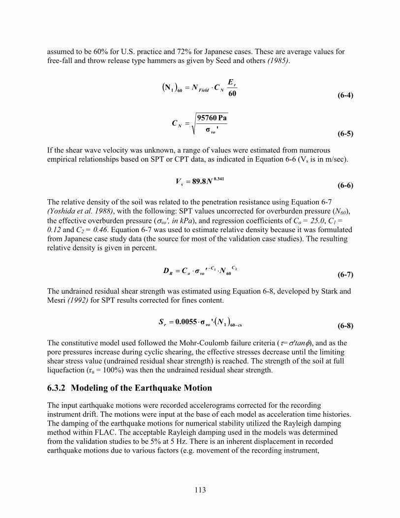
assumed to be 60% for U.S. practice and 72% for Japanese cases. These are average values for free-fall and throw release type hammers as given by Seed and others (1985).

� �

60N 601

rNField

ECN ��

(6-4)

'σPa95760

voNC �

(6-5)

If the shear wave velocity was unknown, a range of values were estimated from numerous empirical relationships based on SPT or CPT data, as indicated in Equation 6-6 (Vs is in m/sec).

(6-6) 0.34189.8NVs �

The relative density of the soil was related to the penetration resistance using Equation 6-7 (Yoshida et al. 1988), with the following: SPT values uncorrected for overburden pressure (N60), the effective overburden pressure (�vo′, in kPa), and regression coefficients of Co = 25.0, C1 = 0.12 and C2 = 0.46. Equation 6-7 was used to estimate relative density because it was formulated from Japanese case study data (the source for most of the validation case studies). The resulting relative density is given in percent.

(6-7) 21

60CC

vooR N'σCD ����

The undrained residual shear strength was estimated using Equation 6-8, developed by Stark and Mesri (1992) for SPT results corrected for fines content.

(6-8) � � s601'σ0.0055 cvor NS�

���

The constitutive model used followed the Mohr-Coulomb failure criteria (�=�′tan�), and as the pore pressures increase during cyclic shearing, the effective stresses decrease until the limiting shear stress value (undrained residual shear strength) is reached. The strength of the soil at full liquefaction (ru = 100%) was then the undrained residual shear strength.

6.3.2 Modeling of the Earthquake Motion

The input earthquake motions were recorded accelerograms corrected for the recording instrument drift. The motions were input at the base of each model as acceleration time histories. The damping of the earthquake motions for numerical stability utilized the Rayleigh damping method within FLAC. The acceptable Rayleigh damping used in the models was determined from the validation studies to be 5% at 5 Hz. There is an inherent displacement in recorded earthquake motions due to various factors (e.g. movement of the recording instrument,

113

permanent earthquake displacements), and is termed baseline shift. The baseline shift has been removed from all of the presented FLAC displacements.

6.3.3 Modeling of the Water

The water in front of slopes was modeled indirectly by including the resulting water pressures along the boundaries. This allows a simple modeling of the water, but does not account for the dynamic interaction of the slope and water. The water within the soil was modeled directly and was allowed to flow during the static solutions. During the dynamic solutions, excess pore pressures were allowed to generate, but the dissipation of these pore pressures was not modeled (as previously addressed).

6.3.4 Boundary Conditions

The boundary conditions for the static solutions consisted of the bottom boundary being fixed in both the horizontal and vertical directions, while the sides of the model were treated as rollers (by fixing only the horizontal direction). During the dynamic analysis the bottom boundary was freed in the horizontal direction to allow application of the horizontal acceleration, and the sidewalls were treated as an infinite medium (free field), having the same properties as the adjacent model perimeter zones. The lateral dimensions of the model were determined as optimum from the results of prior validation case studies as five to seven times the total embankment height in the approach fill and three times the total embankment height in front of the embankment slope.

6.4 VALIDATION OF NUMERICAL MODEL

The use of FLAC for the seismic modeling of earth structures with and without soil improvement required that it be validated and calibrated. Given the rather widespread use of this tool in geotechnical engineering practice, numerous studies have been performed to assess the strengths and limitations of the model. These investigations have focused on the accuracy of the computed seismically-induced deformations as compared to the permanent deformations measured in well documented case studies. Pertinent investigations are shown below.

� Earth structures and liquefaction hazards (Inel et al.1993; Roth et al. 1993; Beaty and Byrne 1998).

� Gravity retaining walls in unimproved and improved soils (Dickenson and Yang 1998). � Anchored sheet pile walls in unimproved and improved soils (McCullough and

Dickenson 1998). � Pile supported wharf structures (Yang 1999). � Behavior of spread footings founded on competent soils underlain by liquefiable soil

(Naesgaard et al. 1998). � Direct comparison with dynamic centrifuge models of earth slopes (Roth et al. 1986,

1993). The strengths and limitations of the numerical model have been well documented in these recent publications. The nuances of the constitutive model and pore pressure generation scheme as

114

applied to liquefaction studies also have been well addressed. The model provides representative displacements for a variety of geotechnical applications. These investigations have focused in limited deformations associated with soil liquefaction (lateral spreading) and not catastrophic flow failures that occur along slopes when the post-earthquake, static shear stresses exceed the residual undrained strength of the soil (as is common in offshore applications involving sensitive soils on submarine slopes). This investigation was confined to cases involving limited ground failures and lateral spreading.

115

7.0 DEFORMATION ANALYSIS OF EMBANKMENTS

7.1 INTRODUCTION

The application of performance-based seismic design specifications is becoming routine for transportation applications. Requisite input for this method design includes the definition of limit states for the structure and/or components being evaluated (allowable force-deformation limits). As applied to embankments and approach fills tolerable permanent deformations are defined. Therefore, engineers require practice-oriented design tools for evaluating earthquake-induced deformations of earth structures. Simplified procedures for estimating deformations of slopes in competent soils have been well developed over the past three decades. However, equivalent methods are still in development for estimating displacements of earth structures built with or on soils that lose appreciable strength during earthquake shaking. Also, at many bridge sites the prevalence of weak soils necessitates the application of soil improvement for mitigating seismic and geologic hazards.

In order to effectively retrofit a bridge foundation sited on or adjacent to liquefiable soil deposits, it is necessary to determine the location and lateral extent of the soil that should be treated by ground improvement techniques. Clearly, the cost and effectiveness of the ground treatment will depend on the volume of soil to be improved. There are currently few guidelines for relating the volume of soil treatment to the anticipated seismic performance of earth structures. Predicting the amount of deformation at a site and the extent and effectiveness of the soil improvement requires a method for evaluating the deformation produced by the earthquake before and after ground treatment. Since acceptable performance is usually defined in terms of limiting deformations below some critical value, assessment of ground improvement strategies depends on the engineer’s ability to analyze likely deformations of deposits including liquefiable soils.

Guidelines for evaluating both the magnitude and pattern of deformations of earth structures caused by strong ground motions are limited. Traditionally, the static factor of safety (FS) computed using limit equilibrium procedures has been used as an indicator of the anticipated seismic slope stability. These analyses often employ a lateral inertial force intended to represent the effects of the earthquake motions on the stability of the slope. The pseudostatic methods of analysis and the associated sliding-block deformation procedures have been described in the literature (Kramer 1996) and will not be thoroughly addressed here. Primary limitations of the pseudostatic method of analysis for performance-based design are that: (1) the influence of excess pore pressure generation on the strength of the soil can only be handled in a de-coupled manner; (2) the relative motion of the slide mass is confined to a single slip plane therefore the pattern of deformations cannot be assessed directly; (3) the sliding block method cannot be applied for cases with static and/or dynamic FS < 1; and (4) the sliding block method can result in negligible permanent displacements for cases where the yield acceleration has not been exceeded, despite evidence that soil yielding prior to reaching the limit state can result in significant deformations. The latter two topics will be addressed in subsequent sections of this chapter. These limitations can be overcome with the use of numerical modeling procedures.

117

Although numerical models are more readily adaptable to site-specific conditions and soil-structure interaction, they generally require substantial geotechnical data and can involve significant time and expense. The numerical models are often impractical for preliminary evaluations of earth structures, final design of low- to moderate-priority structures, and routine soil improvement applications.

Primary objectives of this project were to develop practice-oriented guidelines for evaluating the seismic performance of earth structures founded on liquefiable soils, and to evaluate the effectiveness of ground improvement strategies at bridge sites. The results from advanced numerical dynamic effective stress analyses were compared to more standard methods in order to evaluate the suitability of the simplified methods in predicting ground deformations. The objectives of this comparison include: (1) to identify trends that might allow the results of the simplified, standard-of-practice methods to be modified to better approximate the results of more sophisticated and representative numerical modeling; (2) to identify significant limitations in the standard methods; (3) to develop a simplified approach for estimating lateral deformations of bridge abutments and embankments with and without soil improvement; and (4) to provide recommendations for displacement-based analyses of earth structures.

7.2 ANALYSIS METHODS FOR ESTIMATING DISPLACEMENTS

7.2.1 Introduction

Large lateral displacements of bridge abutments located on liquefiable soils have been documented following numerous recent earthquakes (see Chapter 2 and the appendix). These ground failures have primarily been associated with deformations in the underlying loose saturated sands. In order to mitigate the hazards associated with these large displacements, the soil beneath the abutment must be improved. The engineering challenge is to determine the optimal extent and location of the required soil improvement. Several analysis methods exist for estimating earthquake-induced displacements. Traditional limit equilibrium slope stability analyses can be modified to account for the lateral inertial force induced by the earthquake (pseudostatic analysis). From this analysis, the acceleration required to bring the factor of safety against sliding to unity (yield acceleration) can be determined. Once the yield acceleration has been found, a suite of appropriate acceleration time histories can be obtained and a rigid body, sliding block analyses performed (Newmark-type analyses). Simplified charts have been developed (Makdisi and Seed 1978) for estimating lateral displacements based on Newmark sliding block procedures.

Advanced numerical modeling techniques are also available for predicting earthquake-induced displacements. These techniques are capable of generating deformation patterns and also have the ability to perform coupled effective stress analyses thereby accounting for excess pore pressure generation. The analysis methods mentioned above have their own inherent advantages and limitations. These methods are discussed in the following sections.

7.2.2 Pseudostatic Methods of Analysis for Competent Soils

Standard, limit equilibrium methods for analyzing the static and dynamic stability of slopes are routinely used. The advantage that they have include: (1) the techniques are familiar to most

118

engineers; (2) requisite input includes standard geotechnical parameters that are obtained during routine foundation investigations; and (3) the methods have been coded in straightforward, efficient computer programs that allow for sensitivity studies of various design options.

For use in determining the seismic stability of slopes, limit equilibrium analyses are modified slightly with the addition of a permanent lateral body force that is the product of a seismic coefficient and the mass of the soil bounded by the potential slip. The seismic coefficient (usually designated as kh or Nh) is specified as a fraction of the peak horizontal acceleration, due to the fact that the lateral inertial force is applied for only a short time interval during transient earthquake loading. Seismic coefficients are commonly specified as roughly 1/3 to 1/2 of the peak horizontal acceleration value (Seed 1979; Marcuson et al. 1992; CDMG 1997).

In most cases involving soils that do not exhibit strength loss after the peak strength has been mobilized, common pseudostatic, rigid body methods of evaluation will generally suffice for evaluating the stability of slopes. These methods are well established in the literature (Kramer 1996). Although they are useful for indicating an approximate level of seismic stability in terms of a factor of safety against failure, pseudostatic methods suffer from several potentially important limitations. These are: (1) they do not indicate the range of slope deformations that may be associated with various factors of safety; (2) the influence of excess pore pressure generation on the strength of the soils is incorporated in only a very simplified, “decoupled” manner; (3) progressive deformations that may result due to cyclic loading at stresses less than those required to reduce specific factors of safety to unity are not modeled; (4) strain softening behavior for liquefiable soils or sensitive clays is not directly accounted for, and (5) the dynamic behavior of the slide mass is not accounted for (Kramer and Smith 1997).

7.2.3 Analysis of the “Post-Earthquake” Factor of Safety for Slopes

Traditional slope stability analyses for seismic conditions depend on the overall pseudo-static factor of safety to indicate whether the slope will remain in equilibrium. While these stability analyses do not provide explicit information on the magnitude of seismically-induced deformations, one would expect that slopes with greater pseudo-static stability would be less prone to movement. Therefore, the factor of safety based on this procedure might provide a useful index. As previously mentioned, the pseudostatic methods are particularly useful for cases involving competent soils that do not lose significant strength during shaking. These methods are not, however, well suited for analysis involving liquefiable sandy soils and sensitive fine-grained soils that experience a reduction of strength during seismic loading.

In order to evaluate the seismic stability of slopes involving liquefiable soils using standard limit equilibrium methods, the residual undrained shear strength of the soil can be estimated based on standard geotechnical parameters such as the penetration resistance of the soil based on in situ tests (Figures 4-3 and 4-4). The shear strengths provided in these two figures are applicable only if the seismic loading was sufficient to liquefy sandy soil. Once the residual shear strength of the sandy soil has been estimated, the layer is now modeled in a manner similar to that of an undrained cohesive soil. The dynamic stability (sometimes termed the post-earthquake stability) of the slope can now be assessed. While these equilibrium analyses are relatively simple to perform, this technique for evaluating seismic stability is still based on rigid body mechanics and thus suffers from the same shortcomings as the pseudostatic method.

119

It should be noted that the terms residual strength (Sr, Sus), steady/critical state strength (Su(CRITICAL)) and mobilized residual strength are all used in the literature to describe the shear strength of sandy soils that have experienced liquefaction. The proceedings of the workshop, Shear Strength of Liquefied Soils (Stark et al. 1997) provide the most recent overview of this topic and the significance of the various nomenclatures is addressed. The term, undrained residual strength, will be used in this report and denoted as Sr.

7.2.4 Limited Deformation Analysis

The Newmark methods introduced in Chapter 4 have been widely adopted in engineering due to their simplicity and validation in many earthquake case studies. As evident in Figure 4.10, key parameters related to the soil strength and static slope stability (ky, or ay), input ground motions (kmax), and the duration of ground shaking (as related to the earthquake magnitude) are incorporated into the procedure. The frequency characteristics of the ground motions are not addressed, and the influence of ground motion duration is perhaps over-simplified. As a means of enhancing the simplified chart-based deformation analyses, Jibson (1993) employed the Arias Intensity of the acceleration time history as the primary ground motion parameter for use in a chart solution (Figure 7.1).

Figure 7.1: Newmark Displacement as a Function of Arias Intensity for Several Values of Critical Acceleration

(Jibson 1993)

The Arias Intensity is the integral over time of the square of acceleration, as expressed in Equation 7-1. It has units of velocity (L/T) and can be calculated for each directional component of a strong motion record (Jibson 1993; Kramer 1996). It is a measure of total shaking intensity and is independent of the critical acceleration. This method is not necessarily founded on a theoretical basis given that the deformation of a slope is only a result of acceleration values that exceed the critical acceleration value.

120

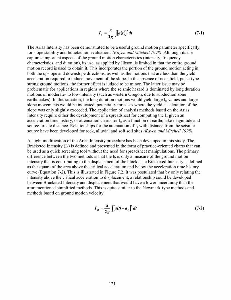
� �� ��� dttagπI a

2

2 (7-1)

The Arias Intensity has been demonstrated to be a useful ground motion parameter specifically for slope stability and liquefaction evaluations (Kayen and Mitchell 1998). Although its use captures important aspects of the ground motion characteristics (intensity, frequency characteristics, and duration), its use, as applied by Jibson, is limited in that the entire ground motion record is used to obtain it. This incorporates the portion of the ground motion acting in both the upslope and downslope directions, as well as the motions that are less than the yield acceleration required to induce movement of the slope. In the absence of near-field, pulse-type strong ground motions, the former effect is judged to be minor. The latter issue may be problematic for applications in regions where the seismic hazard is dominated by long duration motions of moderate- to low-intensity (such as western Oregon, due to subduction zone earthquakes). In this situation, the long duration motions would yield large Ia-values and large slope movements would be indicated, potentially for cases where the yield acceleration of the slope was only slightly exceeded. The application of analysis methods based on the Arias Intensity require either the development of a spreadsheet for computing the Ia given an acceleration time history, or attenuation charts for Ia as a function of earthquake magnitude and source-to-site distance. Relationships for the attenuation of Ia with distance from the seismic source have been developed for rock, alluvial and soft soil sites (Kayen and Mitchell 1998).

A slight modification of the Arias Intensity procedure has been developed in this study. The Bracketed Intensity (Ib) is defined and presented in the form of practice-oriented charts that can be used as a quick screening tool without the need for spreadsheet manipulations. The primary difference between the two methods is that the Ib is only a measure of the ground motion intensity that is contributing to the displacement of the block. The Bracketed Intensity is defined as the square of the area above the critical acceleration and below the acceleration time history curve (Equation 7-2). This is illustrated in Figure 7.2. It was postulated that by only relating the intensity above the critical acceleration to displacement, a relationship could be developed between Bracketed Intensity and displacement that would have a lower uncertainty than the aforementioned simplified methods. This is quite similar to the Newmark-type methods and methods based on ground motion velocity.

� �� �� dtaa(t)gπI cB

2

2 (7-2)

121

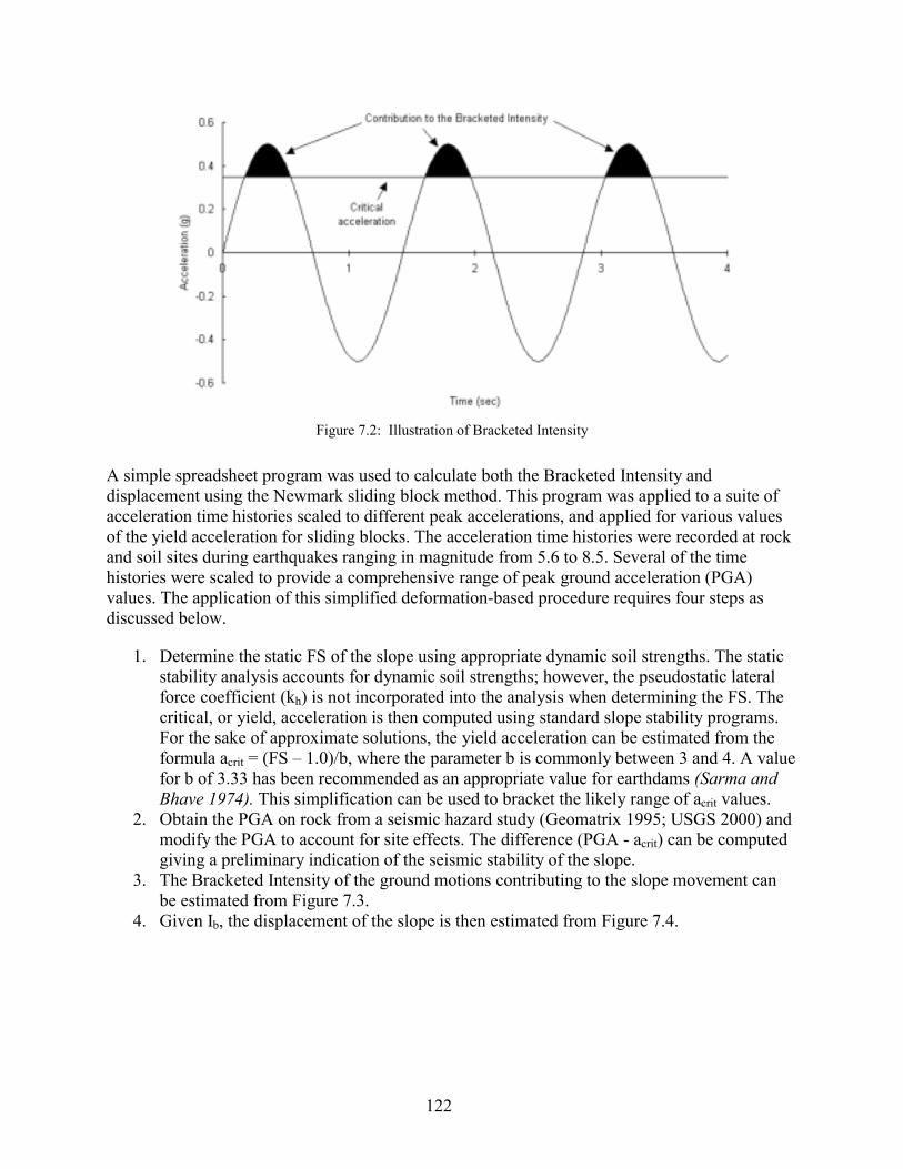
Figure 7.2: Illustration of Bracketed Intensity

A simple spreadsheet program was used to calculate both the Bracketed Intensity and displacement using the Newmark sliding block method. This program was applied to a suite of acceleration time histories scaled to different peak accelerations, and applied for various values of the yield acceleration for sliding blocks. The acceleration time histories were recorded at rock and soil sites during earthquakes ranging in magnitude from 5.6 to 8.5. Several of the time histories were scaled to provide a comprehensive range of peak ground acceleration (PGA) values. The application of this simplified deformation-based procedure requires four steps as discussed below.

1. Determine the static FS of the slope using appropriate dynamic soil strengths. The static stability analysis accounts for dynamic soil strengths; however, the pseudostatic lateral force coefficient (kh) is not incorporated into the analysis when determining the FS. The critical, or yield, acceleration is then computed using standard slope stability programs. For the sake of approximate solutions, the yield acceleration can be estimated from the formula acrit = (FS – 1.0)/b, where the parameter b is commonly between 3 and 4. A value for b of 3.33 has been recommended as an appropriate value for earthdams (Sarma and Bhave 1974). This simplification can be used to bracket the likely range of acrit values.

2. Obtain the PGA on rock from a seismic hazard study (Geomatrix 1995; USGS 2000) and modify the PGA to account for site effects. The difference (PGA - acrit) can be computed giving a preliminary indication of the seismic stability of the slope.

3. The Bracketed Intensity of the ground motions contributing to the slope movement can be estimated from Figure 7.3.

4. Given Ib, the displacement of the slope is then estimated from Figure 7.4.

122

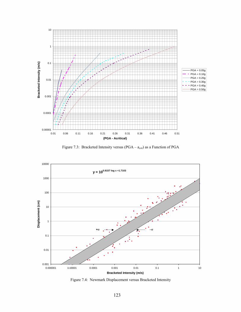
0.00001

0.0001

0.001

0.01

0.1

1

10

0.01 0.06 0.11 0.16 0.21 0.26 0.31 0.36 0.41 0.46 0.51

(PGA - Acritical)

Bra

cket

ed In

tens

ity (m

/s)

PGA = 0.05gPGA = 0.10gPGA = 0.20gPGA = 0.30gPGA = 0.40gPGA = 0.50g

Figure 7.3: Bracketed Intensity versus (PGA – acrit) as a Function of PGA

0.001

0.01

0.1

1

10

100

1000

10000

0.000001 0.00001 0.0001 0.001 0.01 0.1 1 10

Bracketed Intensity (m/s)

Dis

plac

emen

t (cm

)

y = 100.9157 log x +1.7103

+� ��

Figure 7.4: Newmark Displacement versus Bracketed Intensity

123

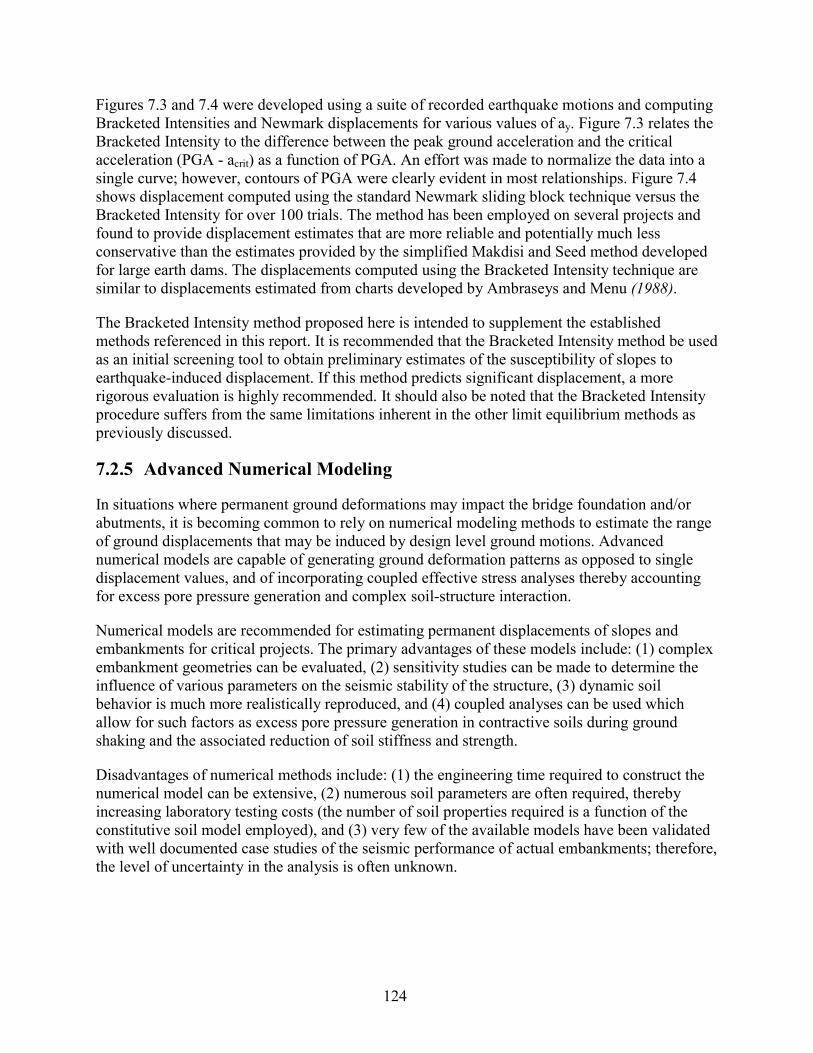
Figures 7.3 and 7.4 were developed using a suite of recorded earthquake motions and computing Bracketed Intensities and Newmark displacements for various values of ay. Figure 7.3 relates the Bracketed Intensity to the difference between the peak ground acceleration and the critical acceleration (PGA - acrit) as a function of PGA. An effort was made to normalize the data into a single curve; however, contours of PGA were clearly evident in most relationships. Figure 7.4 shows displacement computed using the standard Newmark sliding block technique versus the Bracketed Intensity for over 100 trials. The method has been employed on several projects and found to provide displacement estimates that are more reliable and potentially much less conservative than the estimates provided by the simplified Makdisi and Seed method developed for large earth dams. The displacements computed using the Bracketed Intensity technique are similar to displacements estimated from charts developed by Ambraseys and Menu (1988).

The Bracketed Intensity method proposed here is intended to supplement the established methods referenced in this report. It is recommended that the Bracketed Intensity method be used as an initial screening tool to obtain preliminary estimates of the susceptibility of slopes to earthquake-induced displacement. If this method predicts significant displacement, a more rigorous evaluation is highly recommended. It should also be noted that the Bracketed Intensity procedure suffers from the same limitations inherent in the other limit equilibrium methods as previously discussed.

7.2.5 Advanced Numerical Modeling

In situations where permanent ground deformations may impact the bridge foundation and/or abutments, it is becoming common to rely on numerical modeling methods to estimate the range of ground displacements that may be induced by design level ground motions. Advanced numerical models are capable of generating ground deformation patterns as opposed to single displacement values, and of incorporating coupled effective stress analyses thereby accounting for excess pore pressure generation and complex soil-structure interaction.

Numerical models are recommended for estimating permanent displacements of slopes and embankments for critical projects. The primary advantages of these models include: (1) complex embankment geometries can be evaluated, (2) sensitivity studies can be made to determine the influence of various parameters on the seismic stability of the structure, (3) dynamic soil behavior is much more realistically reproduced, and (4) coupled analyses can be used which allow for such factors as excess pore pressure generation in contractive soils during ground shaking and the associated reduction of soil stiffness and strength.

Disadvantages of numerical methods include: (1) the engineering time required to construct the numerical model can be extensive, (2) numerous soil parameters are often required, thereby increasing laboratory testing costs (the number of soil properties required is a function of the constitutive soil model employed), and (3) very few of the available models have been validated with well documented case studies of the seismic performance of actual embankments; therefore, the level of uncertainty in the analysis is often unknown.

124

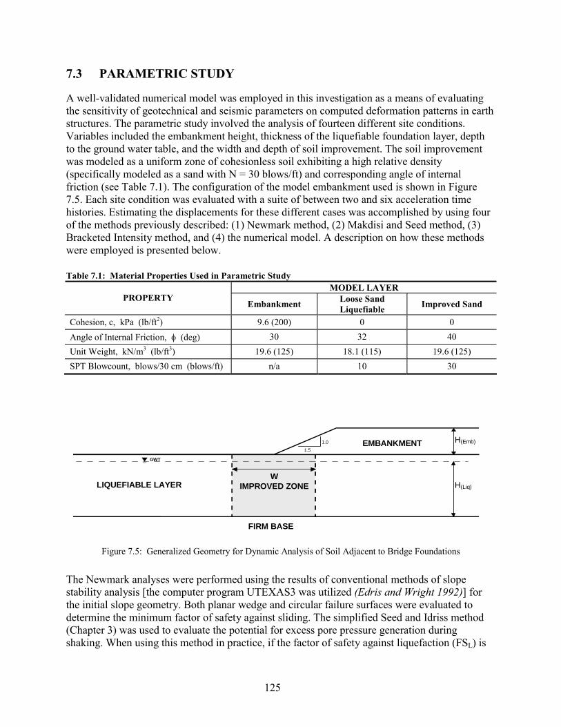
7.3 PARAMETRIC STUDY

A well-validated numerical model was employed in this investigation as a means of evaluating the sensitivity of geotechnical and seismic parameters on computed deformation patterns in earth structures. The parametric study involved the analysis of fourteen different site conditions. Variables included the embankment height, thickness of the liquefiable foundation layer, depth to the ground water table, and the width and depth of soil improvement. The soil improvement was modeled as a uniform zone of cohesionless soil exhibiting a high relative density (specifically modeled as a sand with N = 30 blows/ft) and corresponding angle of internal friction (see Table 7.1). The configuration of the model embankment used is shown in Figure 7.5. Each site condition was evaluated with a suite of between two and six acceleration time histories. Estimating the displacements for these different cases was accomplished by using four of the methods previously described: (1) Newmark method, (2) Makdisi and Seed method, (3) Bracketed Intensity method, and (4) the numerical model. A description on how these methods were employed is presented below.

Table 7.1: Material Properties Used in Parametric Study MODEL LAYER

PROPERTY Embankment Loose Sand

Liquefiable Improved Sand

Cohesion, c, kPa (lb/ft2) 9.6 (200) 0 0

Angle of Internal Friction, � (deg) 30 32 40 Unit Weight, kN/m3 (lb/ft3) 19.6 (125) 18.1 (115) 19.6 (125) SPT Blowcount, blows/30 cm (blows/ft) n/a 10 30

GWT 1.0

1.5

FIRM BASE

LIQUEFIABLE LAYER W

IMPROVED ZONE

EMBANKMENT H(Emb)

H(Liq)

Figure 7.5: Generalized Geometry for Dynamic Analysis of Soil Adjacent to Bridge Foundations

The Newmark analyses were performed using the results of conventional methods of slope stability analysis [the computer program UTEXAS3 was utilized (Edris and Wright 1992)] for the initial slope geometry. Both planar wedge and circular failure surfaces were evaluated to determine the minimum factor of safety against sliding. The simplified Seed and Idriss method (Chapter 3) was used to evaluate the potential for excess pore pressure generation during shaking. When using this method in practice, if the factor of safety against liquefaction (FSL) is

125

found to be high (≥ 1.4 to 1.6), then excess pore pressures are assumed to be small and full soil strength can be used (Marcusen et al. 1990; CDMG 1997). Conversely, if the FSL is low (≤ 1.1), then excess pore pressures will be significant and the residual, undrained strength should be used. A more involved situation occurs when FSL is estimated to be between 1.1 and 1.4. In this case, the excess pore pressure would be estimated from charts relating the excess pore pressure ratio to FSL (Marcuson et al. 1990), and the sand strength would be modified to be somewhere between the static strength and the residual strength.

For this study, only cases that yielded a FSL of less than 1.1 were considered in the development of chart solutions (the residual strength was used for liquefiable soils). The residual strength of the liquefied soil was estimated using vertical effective stresses under the fill, slope, or area beyond the toe of the slope as required, and the formulation for residual undrained strength developed by Stark and Mesri (1992) was employed. Both generalized chart-based solutions and problem-specific double integrations of the acceleration time histories were investigated in this study. The Bracketed Intensity method was also utilized for comparison.

The most sophisticated level of analysis involved two-dimensional numerical modeling of the slope using a commercially available finite difference computer code (FLAC 3.4). This numerical model allowed the input of specific seismic records and stress dependent soil properties as described in Chapter 6. Pertinent output consisted of excess pore pressure generation and deformations within the entire soil mass. This study used the Mohr-Coulomb constitutive model as the starting platform. Pore pressure generation and other pertinent details associated with modeling liquefaction phenomena are also provided in Chapter 6. The seismic strengths for liquefiable soils (Sr) were estimated based on the relationship shown in Figure 4.3.

The main objective of this study was to develop a simplified approach for estimating lateral deformations of embankments with and without soil improvement. To this end, a series of parametric studies were performed using the analysis methods described above. The “post-earthquake” factor of safety obtained using the standard limit equilibrium method and appropriate shear strengths for unimproved sandy soils was compared to the slope deformations computed using sliding block methods as well as the numerical analysis. Since the factor of safety can be thought of as an index of slope stability, it is reasonable to assume that as FS increases, the deformations due to seismic loading of the slope should decrease. Because the performance of the embankment is a function of the earthquake-induced deformations, the factor of safety must be supplemented with a deformation-based method of analysis.

The sliding block methods previously outlined provide an estimate of the slope deformations, however the slide mass is modeled as a perfectly rigid body and the computed deformation applies to the entire mass. It is not possible to discern the pattern of deformations using these methods. The numerical model provides vectors of displacement at grid points in the slope model. The magnitude and direction of the deformations are computed and a contour plot of deformation can be generated for the embankment and affected foundation soils. A direct comparison of the slope deformations computed using the two approaches and numerical modeling method must account for the fact that the numerical model provides the variation of displacement throughout the slope. The deformations computed by the numerical model can be established for any point in the model (e.g., slope crest, toe of slope, selected point in the foundation soil). In this study, the maximum computed deformation is used for comparison with

126

the rigid body methods. The point at which the deformations were the greatest consistently occurred beneath the toe and lower third portion of the slope. This is considered a critical area due to the possible location of abutments, pier foundations, and structural components located upslope.

The differences associated with the various cases are described below.

7.3.1 Embankment Geometry

The generalized geometric configuration of the model was shown in Figure 7.5, but several different configurations were investigated in an attempt to include a range of conditions that exist in the field. Embankment heights of 3 and 9 m were modeled and the thickness of the liquefiable layer was varied from 4.5 to 21 m. The location and width of soil improvement was also investigated. Based on the sensitivity analyses and on constructability issues, the improved soil block was centered about the toe of the slope. Numerical analyses were also performed for sites with no soil improvement. In subsequent analyses the width of the improved block was increased from roughly 4.5 m to a maximum of width of 44 m. In addition to investigating the influence of embankment geometry, the influence of groundwater level was evaluated. For the majority of the study, the groundwater level was modeled to be at the ground surface (top of the liquefiable material) but was lowered to 2 m below the ground surface for some of the cases.

7.3.2 Material Properties

The material properties used in the analyses are shown in Figure 7.5 and summarized in Table 7.1. The liquefiable and improved soils are both cohesionless materials, each layer modeled with uniform density. The embankment was modeled as consisting of compacted clayey sand/sandy clay, common in many field applications. The soil improvement was generally modeled with densification provided by a vibro-compaction method, wherein the loose sandy soil is densified and modeled as a uniform deposit throughout the treated zone. This is a simplification of the actual pattern of densification and the variation in soil density that would be expected from most ground improvement techniques; however, this approach has been used in many case studies.

7.3.3 Ground Motions

Six earthquake motions covering the magnitude range of engineering interest (approximately Mw 6.0 to Mw 8.0) were selected for the parametric study (Table 7.2). The selected acceleration time histories are slightly conservative in the sense that each one is characterized as having greater than average duration for that magnitude, thereby yielding slightly conservative displacement results. All earthquake motions were utilized at their recorded PGA value, with the exception of the 1985 Michoacán record. The latter record was scaled slightly to a PGA of 0.39 g. Plots of the unscaled records are shown in Figure 7.6.

127

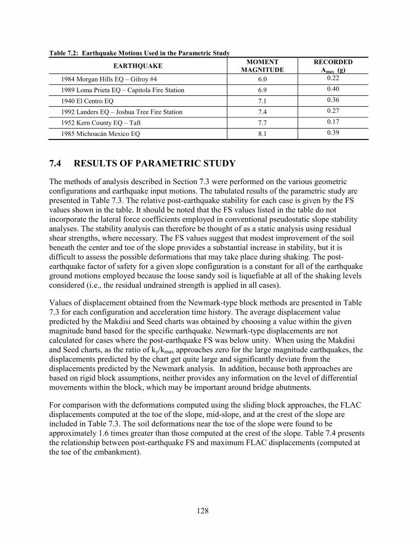
Table 7.2: Earthquake Motions Used in the Parametric Study

EARTHQUAKE MOMENT MAGNITUDE

RECORDED Amax (g)

1984 Morgan Hills EQ – Gilroy #4 6.0 0.22

1989 Loma Prieta EQ – Capitola Fire Station 6.9 0.40

1940 El Centro EQ 7.1 0.36

1992 Landers EQ – Joshua Tree Fire Station 7.4 0.27

1952 Kern County EQ – Taft 7.7 0.17

1985 Michoacán Mexico EQ 8.1 0.39

7.4 RESULTS OF PARAMETRIC STUDY

The methods of analysis described in Section 7.3 were performed on the various geometric configurations and earthquake input motions. The tabulated results of the parametric study are presented in Table 7.3. The relative post-earthquake stability for each case is given by the FS values shown in the table. It should be noted that the FS values listed in the table do not incorporate the lateral force coefficients employed in conventional pseudostatic slope stability analyses. The stability analysis can therefore be thought of as a static analysis using residual shear strengths, where necessary. The FS values suggest that modest improvement of the soil beneath the center and toe of the slope provides a substantial increase in stability, but it is difficult to assess the possible deformations that may take place during shaking. The post-earthquake factor of safety for a given slope configuration is a constant for all of the earthquake ground motions employed because the loose sandy soil is liquefiable at all of the shaking levels considered (i.e., the residual undrained strength is applied in all cases).

Values of displacement obtained from the Newmark-type block methods are presented in Table 7.3 for each configuration and acceleration time history. The average displacement value predicted by the Makdisi and Seed charts was obtained by choosing a value within the given magnitude band based for the specific earthquake. Newmark-type displacements are not calculated for cases where the post-earthquake FS was below unity. When using the Makdisi and Seed charts, as the ratio of ky/kmax approaches zero for the large magnitude earthquakes, the displacements predicted by the chart get quite large and significantly deviate from the displacements predicted by the Newmark analysis. In addition, because both approaches are based on rigid block assumptions, neither provides any information on the level of differential movements within the block, which may be important around bridge abutments.

For comparison with the deformations computed using the sliding block approaches, the FLAC displacements computed at the toe of the slope, mid-slope, and at the crest of the slope are included in Table 7.3. The soil deformations near the toe of the slope were found to be approximately 1.6 times greater than those computed at the crest of the slope. Table 7.4 presents the relationship between post-earthquake FS and maximum FLAC displacements (computed at the toe of the embankment).

128

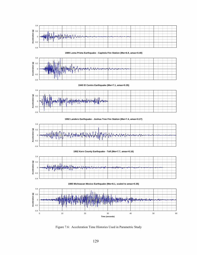
1989 Loma Prieta Earthquake - Capitola Fire Station (Mw=6.9, amax=0.40)

1940 El Centro Earthquake (Mw=7.1, amax=0.35)

-0.4

-0.2

0

0.2

0.4

Acc

eler

atio

n (g

)

-0.4

-0.2

0

0.2

0.4

Acc

eler

atio

n (g

)

-0.4

-0.2

0

0.2

0.4

Acc

eler

atio

n (g

)

1992 Landers Earthquake - Joshua Tree Fire Station (Mw=7.4, amax=0.27)

1952 Kern County Earthquake - Taft (Mw=7.7, amax=0.16)

1985 Michoacan Mexico Earthquake (Mw=8.1, scaled to amax=0.35)

-0.4

-0.2

0

0.2

0.4

Acc

eler

atio

n (g

)

-0.4

-0.2

0

0.2

0.4

Acc

eler

atio

n (g

)

-0.4

-0.2

0

0.2

0.4

0 10 20 30 40 50 6

Time (seconds)

Acc

eler

atio

n (g

)

0

Figure 7.6: Acceleration Time Histories Used in Parametric Study

129

Tab

le 7

.3:

Sum

mar

y of

Mod

el C

onfig

urat

ions

and

Dis

plac

emen

ts fr

om F

LA

C, N

ewm

ark,

Mak

disi

-See

d, a

nd B

rack

eted

Inte

nsity

Typ

e A

naly

ses.

FLA

C D

ispl

acem

ents

(m)

Embankment Height (m)

Depth of Liquefiable Mat) erial (m

omp

ed acem

Widthf Irovement (m)

Ground Water Elevation (m)

Earthquake Motion

Post EQ Factor of Safety

Toe

Mid

Crest

ky

Newmark Displacements (m)

Makdisi-SeDisplents (m)

Bracketed Intensity Displacements (m)

3.05

15.2

40.

00-1

.98

capi

tola

0.46

1.23

1.22

1.01

0.00

--

- 3.

05

15.2

40.

00-1

.98

land

ers

0.46

1.25

1.24

1.12

0.00

--

-3.

05

15.2

40.

00-1

.98

mex

ico

0.46

1.52

1.51

1.25

0.00

--

-3.

05

15.2

46.

10-1

.98

capi

tola

1.6

0.57

-0.5

50.

290.

040.

750.

900.

303.

05

15.2

46.

10-1

.98

land

ers

1.6

0.66

0.65

0.28

0.04

0.91

1.00

0.21

3.05

15

.24

6.10

-1.9

8m

exic

o1.

60.

750.

730.

370.

041.

718.

000.

213.

05

15.2

418

.29

-1.9

8ca

pito

la2.

210.

220.

210.

220.

640.

000.

000.

003.

05

15.2

418

.29

-1.9

8la

nder

s2.

210.

130.

120.

130.

640.

000.

000.

003.

05

15.2

418

.29

-1.9

8m

exic

o2.

210.

200.

190.

210.

640.

000.

000.

003.

05

15.2

40.

000.

00ca

pito

la0.

462.

082.

081.

740.

00-

--

3.05

15

.24

0.00

0.00

land

ers

0.46

2.41

2.40

2.06

0.00

--

-3.

05

15.2

40.

000.

00m

exic

o0.

462.

442.

432.

050.

00-

--

3.05

15

.24

6.10

0.00

capi

tola

1.48

1.14

1.12

0.67

0.03

0.82

0.95

0.30

3.05

15

.24

6.10

0.00

land

ers

1.48

1.40

1.37

0.77

0.03

1.09

1.00

0.15

3.05

15

.24

6.10

0.00

mex

ico

1.48

1.63

1.57

0.95

0.03

1.37

9.00

0.21

3.05

15

.24

18.2

90.

00ca

pito

la2.

080.

420.

370.

420.

560.

000.

000.

003.

05

15.2

418

.29

0.00

land

ers

2.08

0.42

0.35

0.41

0.56

0.00

0.00

0.00

3.05

15

.24

18.2

90.

00m

exic

o2.

080.

570.

480.

540.

560.

000.

000.

009.

14

4.57

0.00

0.00

capi

tola

0.21

3.43

2.98

2.19

0.00

--

-9.

14

4.57

0.00

0.00

el c

entro

0.21

3.93

3.52

2.42

0.00

--

-9.

14

4.57

0.00

0.00

land

ers

0.21

5.00

4.29

3.26

0.00

--

-9.

14

4.57

0.00

0.00

mex

ico

0.21

5.89

5.29

4.04

0.00

--

-9.

14

4.57

0.00

0.00

mor

gan

hills

0.21

0.77

0.34

0.41

0.00

--

-9.

14

4.

570.

000.

00ta

ft 0.

212.

231.

671.

330.

00-

--

9.14

4.

576.

100.

00ca

pito

la0.

752.

062.

421.

510.

00-

--

9.14

4.

576.

100.

00la

nder

s0.

752.

603.

082.

090.

00-

--

9.14

4.

576.

100.

00m

exic

o0.

753.

543.

922.

730.

00-

--

9.14

4.

576.

100.

00m

orga

n hi

lls0.

750.

180.

150.

120.

00-

--

9.14

4.57

6.10

0.00

taft

0.75

1.31

1.55

0.95

0.00

--

-

130

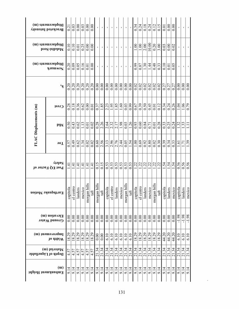
131

FLA

C D

ispl

acem

ents

(m)

Embankment Height (m)

Depth of Liquefiable Mat) erial (m

omp

ed acem

Earthquake Motion

Widthf Irovement (m)

Ground Water Elevation (m)

Post EQ Factor of Safety

Toe

Mid

Crest

9.14

4.

5718

.29

0.00

capi

tola

1.41

0.57

0.50

0.28

0.20

0.20

0.10

0.21

9.14

4.

5718

.29

0.00

el c

entro

1.41

0.49

0.43

0.18

0.20

0.09

0.10

0.03

9.14

4.

5718

.29

0.00

land

ers

1.41

0.62

0.62

0.36

0.20

0.05

0.01

0.00

9.14

4.

5718

.29

0.00

mex

ico

1.41

1.34

1.13

0.62

0.20

0.16

0.25

0.03

9.14

4.

5718

.29

0.00

mor

gan

hills

1.41

0.02

0.01

0.00

0.20

0.01

0.00

0.00

9.14

4.57

18.2

90.

00ta

ft 1.

410.

020.

020.

200.

000.

000.

009.

14

21.3

40.

000.

00m

orga

n hi

lls0.

150.

600.

280.

370.

00-

--

9.14

21.3

40.

000.

00ta

ft 0.

152.

562.

261.

850.

00-

--

9.14

21

.34

6.10

0.00

capi

tola

0.53

3.13

2.64

2.23

0.00

--

-9.

14

21.3

46.

100.

00el

cen

tro0.

532.

962.

321.

950.

00-

--

9.14

21

.34

6.10

0.00

land

ers

0.53

2.76

2.17

1.85

0.00

--

-9.

14

21.3

46.

100.

00m

exic

o0.

532.

441.

981.

600.

00-

--

9.14

21

.34

6.10

0.00

mor

gan

hills

0.53

0.05

0.03

0.03

0.00

--

-9.

14

21

.34

6.10

0.00

taft

0.53

1.54

1.26

0.99

0.00

--

-9.

14

21.3

418

.29

0.00

capi

tola

1.22

1.00

0.93

0.67

0.02

0.99

1.00

0.34

9.14

21

.34

18.2

90.

00el

cen

tro1.

220.

690.

600.

390.

020.

871.

000.

249.

14

21.3

418

.29

0.00

land

ers

1.22

0.92

0.84

0.50

0.02

1.30

2.00

0.18

9.14

21

.34

18.2

90.

00m

exic

o1.

220.

800.

710.

450.

021.

4410

.00

0.24

9.14

21

.34

18.2

90.

00m

orga

n hi

lls1.

220.

020.

010.

010.

020.

480.

200.

129.

14

21

.34

18.2

90.

00ta

ft 1.

220.

300.

280.

120.

020.

333.

000.

159.

14

21.3

444

.20

0.00

capi

tola

1.54

0.39

0.33

0.34

0.27

0.10

0.03

0.01

9.14

21

.34

44.2

00.

00la

nder

s1.

540.

340.

250.

240.

270.

010.

000.

009.

14

21.3

444

.20

0.00

mex

ico

1.54

0.33

0.24

0.26

0.27

0.05

0.02

0.00

9.14

21

.34

6.10

-1.9

8ca

pito

la0.

561.

611.

321.

040.

00-

--

9.14

21

.34

6.10

-1.9

8la

nder

s0.

561.

711.

331.

060.

00-

--

9.14

21

.34

6.10

-1.9

8m

exic

o0.

561.

391.

110.

790.

00-

--Bracketed Intensity

Displacements (m)

Newmark Displacements (m)

Makdisi-SeDisplents (m)

ky

0.01

.

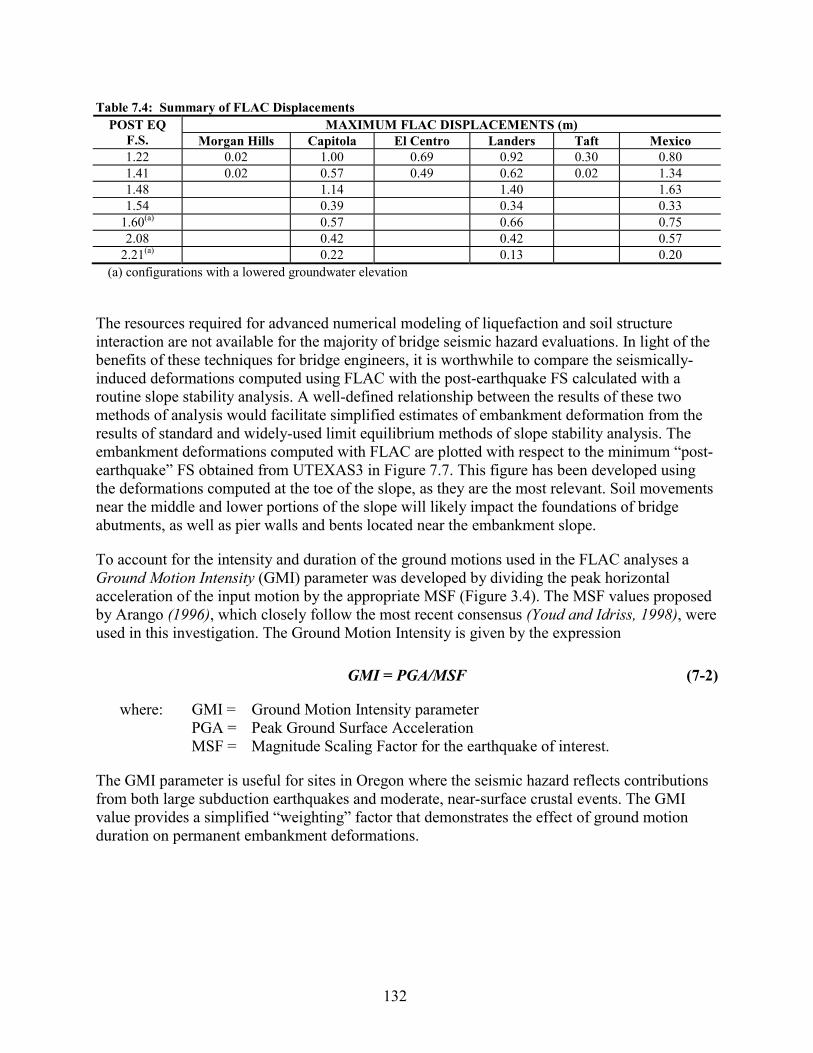
Table 7.4: Summary of FLAC Displacements MAXIMUM FLAC DISPLACEMENTS (m) POST EQ

F.S. Morgan Hills Capitola El Centro Landers Taft Mexico 1.22 0.02 1.00 0.69 0.92 0.30 0.80 1.41 0.02 0.57 0.49 0.62 0.02 1.34 1.48 1.14 1.40 1.63 1.54 0.39 0.34 0.33

1.60(a) 0.57 0.66 0.75 2.08 0.42 0.42 0.57

2.21(a) 0.22 0.13 0.20 (a) configurations with a lowered groundwater elevation

The resources required for advanced numerical modeling of liquefaction and soil structure interaction are not available for the majority of bridge seismic hazard evaluations. In light of the benefits of these techniques for bridge engineers, it is worthwhile to compare the seismically-induced deformations computed using FLAC with the post-earthquake FS calculated with a routine slope stability analysis. A well-defined relationship between the results of these two methods of analysis would facilitate simplified estimates of embankment deformation from the results of standard and widely-used limit equilibrium methods of slope stability analysis. The embankment deformations computed with FLAC are plotted with respect to the minimum “post-earthquake” FS obtained from UTEXAS3 in Figure 7.7. This figure has been developed using the deformations computed at the toe of the slope, as they are the most relevant. Soil movements near the middle and lower portions of the slope will likely impact the foundations of bridge abutments, as well as pier walls and bents located near the embankment slope.

To account for the intensity and duration of the ground motions used in the FLAC analyses a Ground Motion Intensity (GMI) parameter was developed by dividing the peak horizontal acceleration of the input motion by the appropriate MSF (Figure 3.4). The MSF values proposed by Arango (1996), which closely follow the most recent consensus (Youd and Idriss, 1998), were used in this investigation. The Ground Motion Intensity is given by the expression

GMI = PGA/MSF (7-2)

where: GMI = Ground Motion Intensity parameter PGA = Peak Ground Surface Acceleration

MSF = Magnitude Scaling Factor for the earthquake of interest.

The GMI parameter is useful for sites in Oregon where the seismic hazard reflects contributions from both large subduction earthquakes and moderate, near-surface crustal events. The GMI value provides a simplified “weighting” factor that demonstrates the effect of ground motion duration on permanent embankment deformations.

132

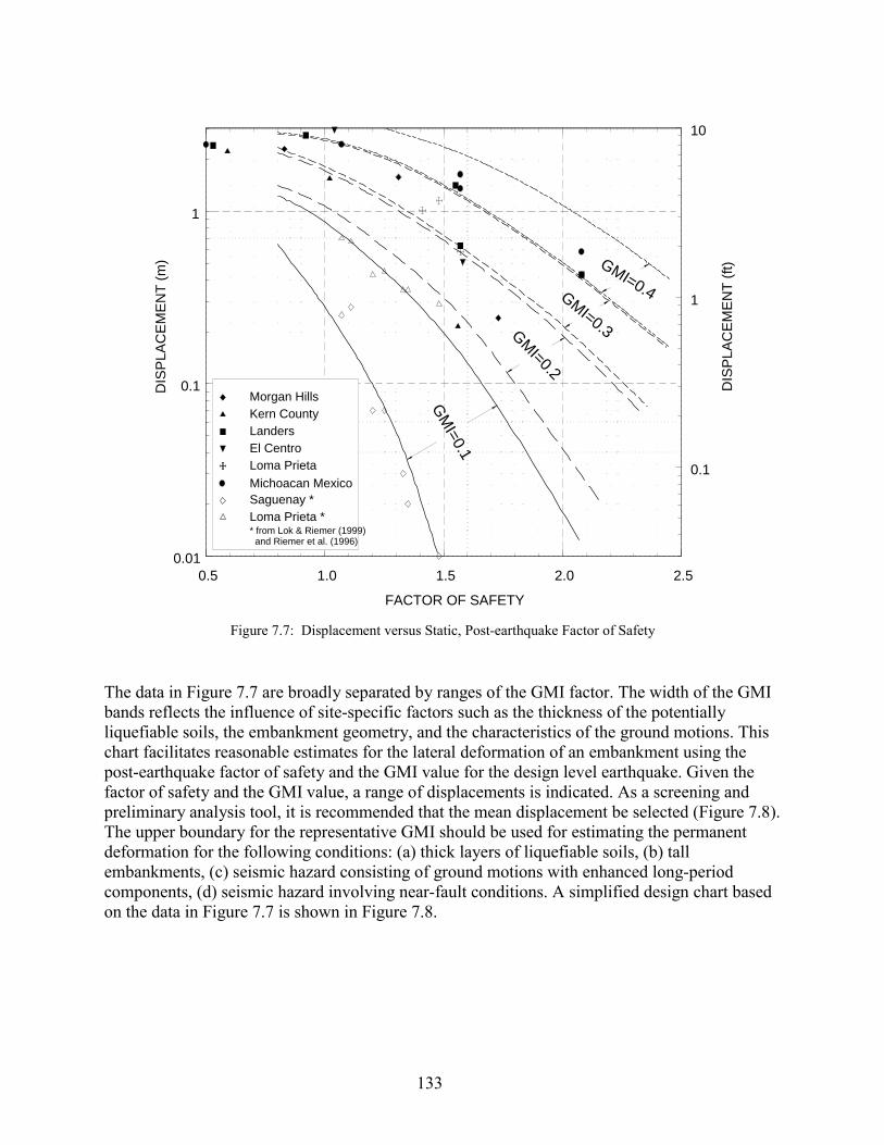
0.5 1.0 1.5 2.0 2.5

FACTOR OF SAFETY

DIS

PLAC

EMEN

T (ft

)

0.1

1

10

0.01

0.1

1

DIS

PLAC

EMEN

T (m

) GMI=0.4

GMI=0.1

GMI=0.2

GMI=0.3

Morgan HillsKern CountyLandersEl CentroLoma PrietaMichoacan MexicoSaguenay *Loma Prieta ** from Lok & Riemer (1999) and Riemer et al. (1996)

Figure 7.7: Displacement versus Static, Post-earthquake Factor of Safety

The data in Figure 7.7 are broadly separated by ranges of the GMI factor. The width of the GMI bands reflects the influence of site-specific factors such as the thickness of the potentially liquefiable soils, the embankment geometry, and the characteristics of the ground motions. This chart facilitates reasonable estimates for the lateral deformation of an embankment using the post-earthquake factor of safety and the GMI value for the design level earthquake. Given the factor of safety and the GMI value, a range of displacements is indicated. As a screening and preliminary analysis tool, it is recommended that the mean displacement be selected (Figure 7.8). The upper boundary for the representative GMI should be used for estimating the permanent deformation for the following conditions: (a) thick layers of liquefiable soils, (b) tall embankments, (c) seismic hazard consisting of ground motions with enhanced long-period components, (d) seismic hazard involving near-fault conditions. A simplified design chart based on the data in Figure 7.7 is shown in Figure 7.8.

133

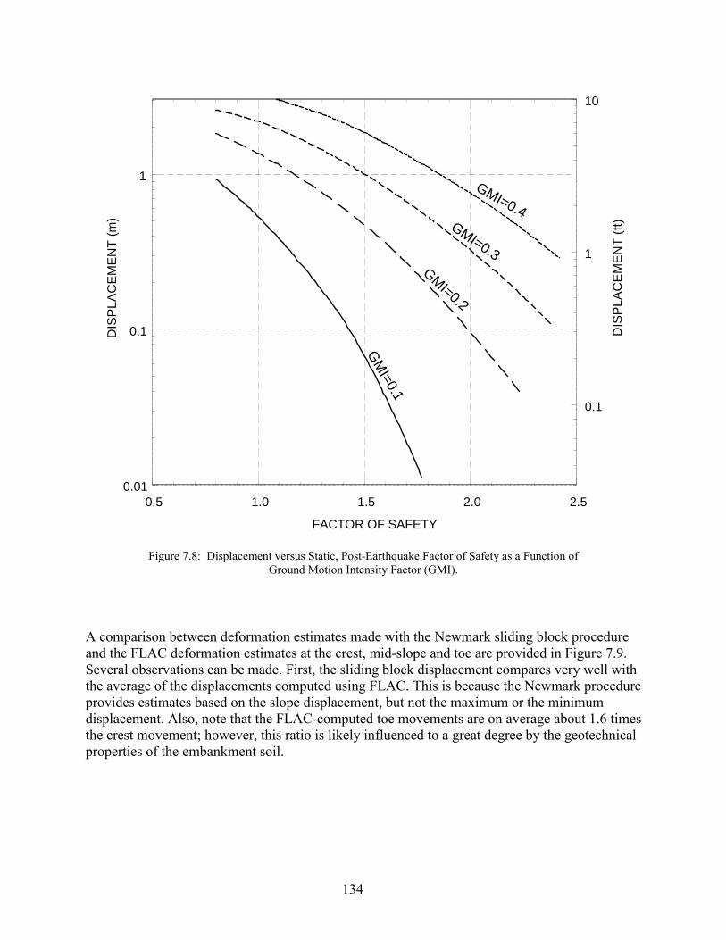
0.5 1.0 1.5 2.0 2.5

FACTOR OF SAFETY

DIS

PLAC

EMEN

T (ft

)

0.1

1

10

0.01

0.1

1

DIS

PLAC

EMEN

T (m

)

GMI=0.4

GMI=0.1

GMI=0.2

GMI=0.3

Figure 7.8: Displacement versus Static, Post-Earthquake Factor of Safety as a Function of

Ground Motion Intensity Factor (GMI).

A comparison between deformation estimates made with the Newmark sliding block procedure and the FLAC deformation estimates at the crest, mid-slope and toe are provided in Figure 7.9. Several observations can be made. First, the sliding block displacement compares very well with the average of the displacements computed using FLAC. This is because the Newmark procedure provides estimates based on the slope displacement, but not the maximum or the minimum displacement. Also, note that the FLAC-computed toe movements are on average about 1.6 times the crest movement; however, this ratio is likely influenced to a great degree by the geotechnical properties of the embankment soil.

134

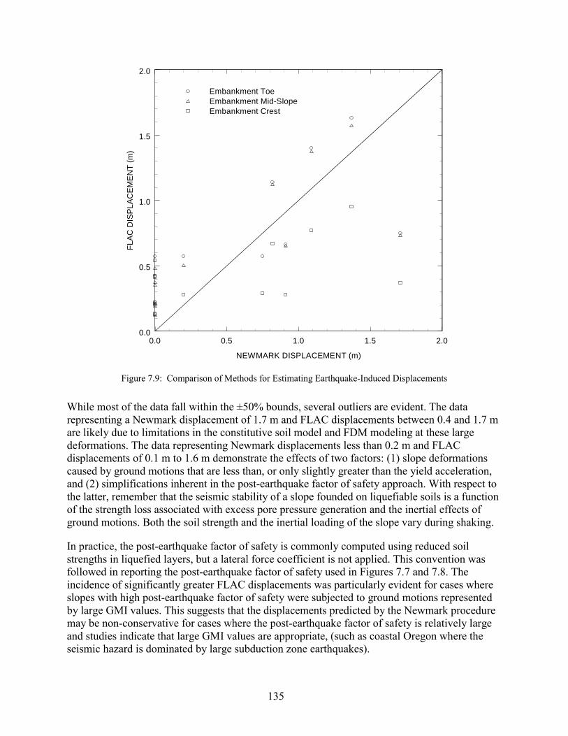
0.0 0.5 1.0 1.5 2.0

NEWMARK DISPLACEMENT (m)

0.0

0.5

1.0

1.5

2.0

FLAC

DIS

PLAC

EM

ENT

(m)

Embankment ToeEmbankment Mid-SlopeEmbankment Crest

Figure 7.9: Comparison of Methods for Estimating Earthquake-Induced Displacements

While most of the data fall within the ±50% bounds, several outliers are evident. The data representing a Newmark displacement of 1.7 m and FLAC displacements between 0.4 and 1.7 m are likely due to limitations in the constitutive soil model and FDM modeling at these large deformations. The data representing Newmark displacements less than 0.2 m and FLAC displacements of 0.1 m to 1.6 m demonstrate the effects of two factors: (1) slope deformations caused by ground motions that are less than, or only slightly greater than the yield acceleration, and (2) simplifications inherent in the post-earthquake factor of safety approach. With respect to the latter, remember that the seismic stability of a slope founded on liquefiable soils is a function of the strength loss associated with excess pore pressure generation and the inertial effects of ground motions. Both the soil strength and the inertial loading of the slope vary during shaking.

In practice, the post-earthquake factor of safety is commonly computed using reduced soil strengths in liquefied layers, but a lateral force coefficient is not applied. This convention was followed in reporting the post-earthquake factor of safety used in Figures 7.7 and 7.8. The incidence of significantly greater FLAC displacements was particularly evident for cases where slopes with high post-earthquake factor of safety were subjected to ground motions represented by large GMI values. This suggests that the displacements predicted by the Newmark procedure may be non-conservative for cases where the post-earthquake factor of safety is relatively large and studies indicate that large GMI values are appropriate, (such as coastal Oregon where the seismic hazard is dominated by large subduction zone earthquakes).

135

The comparisons between the standard Newmark-type analyses and the results of more rigorous numerical modeling suggest that when carefully performed, the simple sliding block method captures the important aspects of the seismic performance of slopes, and provides similar conclusions about the influence of embankment geometry and soil treatment configurations. This observation applies for cases with no embedded structures or piles in the slope. Incorporation of these bridge and foundation elements limits the applicability of the simple sliding block methods, and necessitates the use of numerical soil-structure interaction models. The scatter and uncertainty inherent in all of the simplified approaches must also be noted when evaluating the seismic performance of earth structures such as approach fills, embankments and abutments.

The results of this comparative study are supplemented by the findings of a similar study performed to evaluate the effectiveness of liquefaction remediation measures for bridges (Riemer et al. 1996; Lok and Riemer, 1999). Riemer modeled an embankment and soil profile that was very similar to that studied here. The 2-D FLAC model and the Makdisi and Seed procedure were used to estimate lateral embankment deformations for cases with and without soil improvement by densification. Very good agreement has been found between the results of the two investigations. One important conclusion made from the Riemer study was that the predominant frequency of the design earthquake might have a significant effect on the expected displacements. Low frequency shaking may produce much larger total movements than high frequency shaking for earthquakes of comparable magnitude and duration. This is predominantly due to the greater area under acceleration pulses that exceed the yield acceleration thereby resulting in greater computed Ia, Ib, and displacement.

7.5 CONCLUSIONS

The seismic performance of a variety of embankment configurations were evaluated in sensitivity studies involving different soil profiles, ground treatment configurations, and input ground motions. The effectiveness of the soil improvement was evaluated using standard limit equilibrium slope stability methods combined with rigid body Newmark-type displacement analyses. Supplementary analyses were performed using a well-validated 2-D numerical effective stress model, in order to evaluate the applicability of the more simplified, standard procedures for cases involving soil liquefaction. Based on this study, the following observations and conclusions can be made.

� Simplified Newmark-based methods of evaluation are valuable tools for identifying embankments vulnerable to excessive lateral spreading and seismically-induced deformations, provided that appropriate dynamic soil properties and acceleration time histories are used. It is recommended that these methods be supplemented with more rigorous stability analyses in cases where computed deformations approach allowable limits. Given the inherent variability of the slope displacements estimated using the simplified approaches, and the ease of use of these procedures, it is recommended that two or more of the methods be used on projects requiring preliminary estimates of permanent displacement.

� A simplified four-step method for estimating deformations that is similar to the established method of Makdisi and Seed (1978) has been developed. The proposed method is based on the Bracketed Intensity. This technique has been found to yield

136

suitably reliable estimates of permanent embankment deformation for preliminary screening purposes.

� On the basis of the numerical modeling, the application of ground improvement over a relatively small area beneath the embankment substantially reduces expected seismic deformations. The final configuration of soil improvement at a bridge site will reflect the extent of the liquefiable soil, as well as other key factors related to the cost and benefit of ground treatment (importance of the bridge, level of risk, constructability and access).

� The simplified procedure for estimating embankment deformations developed by Makdisi and Seed tends to yield very large displacements for low critical acceleration ratios (ky/kmax � 0.3). These displacements tend to be much larger than the displacements provided by the other simplified methods referenced herein, often as much as an order of magnitude larger for earthquakes of magnitude > 7. This is consistent with observations made by other investigators (Jibson 1993).

� The 2-D numerical model was used as the basis for a sensitivity study of the influence of geotechnical and seismic parameters on computed deformations. Because relatively few projects warrant sophisticated numerical modeling, a primary objective of the study was to establish a robust relationship between standard slope stability indicators such as the post-earthquake factor of safety with the deformations computed from the more rigorous numerical model. This approach led to the development of a straightforward method for estimating deformations based on standard-of-practice methods of analysis. The deformations estimated using Figures 7.7 and 7.8 are considered more reliable than the broad estimates provided by general Newmark-based design charts. However, the range of uncertainty evinced by the scatter in the data is still significant. This method should be considered a refinement to existing screening tools.

� A simplified method for estimating permanent lateral deformations of embankments based on the post-earthquake factor of safety was developed to facilitate performance-based seismic design incorporating ground improvement to mitigate liquefaction hazards. The results of this work, as well as that of similar recent investigations (Riemer et al. 1996; Cooke and Mitchell, 1999; Lok and Reimer, 1999) demonstrate the potentially significant uncertainty in simplified methods such as these for estimating earthquake-induced deformations of embankments.

� Calculated values of the post-earthquake factor of safety correlate reasonably well with the displacements computed using two-dimensional numerical models. However, this observation should be tempered with consideration of the effects of frequency characteristics of the input motions, the dynamic response of the slope, and the influence of near-fault motions when appropriate.

� In evaluating the results of this investigation, it should be noted that analyses were performed for 2-D, plane-strain conditions. Three-dimensional effects at the edges of approach fills were not explicitly investigated. Clearly, ground treatment must extend beyond the toe of the earth structures in the transverse and longitudinal directions.

137

8.0 HAZARD EVALUATION AND DEVELOPMENT OF MITIGATION STRATEGIES – EXAMPLE PROBLEM

8.1 INTRODUCTION

In order to assist engineers with the application of the individual procedures for evaluating liquefaction hazards, a comprehensive design example has been prepared. This hazard evaluation proceeds in a step-by-step manner, as would be followed in practice. A general flow chart illustrating the overall procedure is provided in Figure 8.1. This chart provides a framework to initiate a liquefaction hazard evaluation and assess the effectiveness of mitigation alternatives. The background material for each stage of the evaluation is referenced in the chart with a chapter and/or section annotation. It should be noted that project-specific conditions may require modifications to the process outlined in the flow chart.

All seismic hazard information, in situ geotechnical data, and laboratory geotechnical soil parameters have been collected for a study site that includes a large levee located along the Columbia River near the Portland International Airport (PDX). This levee is a flood protection structure, as well as an embankment for major roadways and bridge approaches. This site was selected for the following reasons.

1. The prevalence of loose to medium dense sandy and silty soils. 2. The existence of extensive geotechnical data. 3. Fluctuating ground water levels are controlled by the river stage. 4. The seismic hazard includes contributions by large Cascadia subduction zone

earthquakes, deep intra-plate earthquakes, and local shallow crustal sources. 5. The site is located along a major thoroughfare (Marine Drive), and between two major

Columbia River bridges (Interstate 5 and Interstate 205). Also, new bridges are being planned near Hayden Island as part of the Port of Portland’s terminal development.

This example problem is presented in a series of interrelated steps, as it would be performed in practice. The method, as it is outlined here, is also intended to be consistent with the requirements of ODOT’s Liquefaction Mitigation Policy. The following discussion provides background for the regional seismic hazard, representative river stages and flood hazards, and geologic description before addressing specific aspects of the liquefaction evaluation.

The seismic hazard in the Portland region reflects the contributions of three seismic sources: (1) interplate earthquakes along the Cascadia Subduction Zone located near the Pacific coast; (2) relatively deep intraplate subduction zone earthquakes that may be located as far inland as the Portland metropolitan region; and (3) relatively shallow crustal earthquakes located in the Portland metropolitan region. The maximum credible events associated with these source zones are postulated to be in the range of 8.5-9.0, 7.0-7.5, and 6.5-7.0, respectively. The results of recent probabilistic, uniform seismic hazard studies (Geomatrix 1995; USGS 1999; Wong et al. 2000) indicate significant levels of bedrock shaking at recurrence intervals of engineering

139

interest. Specifically, the peak bedrock acceleration having a 10% probability of exceedance in 50 years (i.e., 475 year return period) is approximately 0.2 g along this portion of the Columbia River. These strong ground motions, modified to account for site effects, are clearly capable of initiating liquefaction in the sandy soils that are prevalent along the riverfront.

The acceptable seismic performance of earth structures built adjacent to the river will reflect the sensitivity of bridge structures and ancillary components to the magnitude and pattern of potential soil deformations (e.g.; shallow sloughing, deep-seated failure). Anticipated repair costs for potential failure modes, as well as the consequence of loss of serviceability of key transportation lifelines in the event of a major failure are also primary concerns. Pertinent issues for this example problem are shown below.

� The influence of river stage on the static pore pressures in riverfront embankments and foundation soils, and the variation in seismic performance of the levee as a function of the river level. The static stability of the levee is evaluated at three pertinent river stages (i.e., the water level at the crest of the levee, the 100-year flood elevation, and the summertime, low flow condition).

� The excess pore pressure generation and post-liquefaction behavior of both sandy and silty foundation soils.

� The potential for large permanent deformations or flow failures of the Columbia River sediments.

� The potential for excessive settlement of earth structures due to volumetric changes in the soil following cyclic loading.

� The applicability of the standard sliding block-type analyses presented in this report for estimating earthquake-induced deformations of riverfront embankments.

� The application of a 2D numerical dynamic effective stress model for estimating the seismic performance of riverfront embankments

� The effectiveness of soil improvement for mitigating liquefaction hazards and minimizing earthquake-induced deformations.

8.1.1 Geotechnical Site Characterization

Soils reports provided by the Portland District of the Corps of Engineers and the Port of Portland were reviewed along with information provided by local engineering consulting firms, the Oregon Department of Geology and Mineral Industries (DOGAMI), and the technical literature. This information was supplemented with the results of a more rigorous, site-specific investigation (Dickenson et al. 2000). A total of four exploratory mud-rotary borings, 12 cone penetration (CPT) soundings, and one dilatometer (DMT) sounding were carried out in this complementary investigation. This field investigation provided requisite engineering properties for the geotechnical analyses outlined here. The field investigation was augmented with data from a comprehensive geotechnical laboratory investigation. High quality, thin-walled tube samples and the disturbed split-spoon samples obtained during the field investigation were transported to the Geotechnical Engineering Laboratory at Oregon State University. The following standard laboratory tests were performed: moisture/density, gradation, Atterberg limits, consolidation, direct shear, and triaxial compression tests (TXUU, TXCU). Also, a suite of more sophisticated cyclic triaxial tests were completed.

140

Flow Chart for the Evaluation and Mitigation of Liquefaction Hazards to Bridge Approach Fills

STEP 1Determine Regional Seismic Hazard including

Design-Level Ground Motion Parameters On Bedrock (Section 8.2)

STEP 2Geotechnical Site Characterization

(Section 8.3)

STEP 3Evaluate Site Effects and Determine Ground Surface Motion

(Section 8.4)

STEP 4Preliminary Screening for Liquefaction Hazards

Are Liquefaction Hazards Indicated? (Chapter 3)

STEP 5Quantitative Evaluation of Liquefaction Hazards including:

1. Factor of safety against liquefaction (Sections 8.6 & 8.7) 2. Estimate excess pore pressure generation (Chapter 3) 3. Estimate cyclic strength of cohesionless soils (Chapter 4) 4. Estimate lateral spread displacements (Chapter 4) 5. Estimate surface settlements due to cyclic loading

(Chapter 4)

Are liquefaction hazards potentially damaging to approach embankments and foundations?

Figure 8.1: Flow Chart for Evaluating and Mitigating Liquefaction Hazards

141

Flow Chart for Evaluation and Mitigation of Liquefaction Hazards to Bridge Approach Fills

(page 2)

STEP 6Is remedial ground treatment warranted?

(ODOT Liquefaction Mitigation Policy)

STEP 7ADevelop Liquefaction Mitigation Program including:

1. Select method(s) of remedial soil improvement (Chapter 5) 2. Evaluate constructability issues pertaining to soil

improvement methods (e.g., access, construction vibrations, noise, project duration) Develop preliminary cost estimates for various soil improvement schemes.

STEP 7BEstablish the Extent of Soil Improvement

1. Determine the volume of soil to be treated (iterative seismic performance analysis outlined in Chapter 7)

2. Limit equilibrium methods (static, pseudostatic, sliding-block) a. Effective stress analysis b. Total stress analysis using residual strengths

Has the minimum allowable factor of safety been exceeded?

3. Numerical dynamic effective stress modeling (Chapter 6)

Have soil deformations been reduced to an allowable extent?

Limit states for foundation and bridge elements have not been exceeded?

4. Estimate cost for the preferred soil improvement application.

STEP 8Proceed with Seismic Design of

Approach Embankments, Abutments and Foundations

Apply established methods of analysis and design for competent soils

Figure 8.1 (continued): Flow Chart for Evaluating and Mitigating Liquefaction Hazard

142

8.1.2 Analyses of Seepage and Static Stability of Riverfront Slopes

The static stability of the levee is influenced to a high degree by existing seepage conditions. The seismic performance of the levee also will be affected by the seepage conditions at the time of an earthquake. It would have been advantageous to evaluate the seismic performance of the levee in a probabilistic framework that incorporated hydraulic data with the seismic hazard characteristics of the region. However, this type of coupled, multi-hazard probabilistic analysis was outside the scope of this example. In lieu of a truly probabilistic study, three flow conditions were considered in the investigation: (1) the summertime, low-flow condition, (2) the river level corresponding to the 100-year flow, and (3) the river stage at the crest of the levee. The steady-state seepage conditions and corresponding static stability of the levee was evaluated using commercially available numerical models.

8.1.3 Liquefaction Hazard Analyses

The liquefaction susceptibility of the soils in the levee and foundation were assessed on the basis of the in situ and laboratory data collected. State-of-the-practice methods for evaluating the liquefaction and post-liquefaction behavior of the soils were applied for seismic loading conditions representative of the three primary earthquake hazards in the region. These analyses incorporated the results of recent probabilistic ground motion estimates for bedrock sites using transfer functions computed with one-dimensional dynamic soil response models, and cyclic laboratory data on similar soils at local sites. This investigation focused on excess pore pressure generation, residual undrained shear strengths, and post-cyclic loading volumetric changes of the predominantly silty and sandy deposits.

In order to assess the influence of exposure time on the seismic performance of riverfront embankments, the seismic load levels considered included ground motions having a 2% probability of exceedance in 50 years, and 10% probability of exceedance in 50 years. These recurrence intervals are compatible with hazard evaluations performed by transportation departments in the western United States for bridges of normal and high importance, as well as for recent seismic hazard studies for the region.

8.1.4 Seismic Performance Evaluation

The primary goal was to assess the seismic performance of riverfront embankments at various levels of ground shaking and at different river levels. The performance of the embankment was evaluated in terms of the lateral and vertical deformations resulting from the input ground motions. The potential for lateral spreading and possible flow failures was addressed. The lateral deformations were computed using simplified, empirically-based methods for estimating lateral deformations, and from a limited number of numerical 2D dynamic effective stress analyses. As previously addressed, the numerical model has been used extensively by the principal investigator in seismic performance investigations of waterfront retaining structures, pile supported wharves, and a variety of earth structures. The results of the simplified analyses were compared to the more sophisticated modeling and the strengths and limitations of each method were noted.

143

The deformation evaluations were performed for a levee section considered to be representative of the riverfront between the Interstate 5 and Interstate 205 bridges. The deformation analyses focused only on the response of the levee and foundation soils; therefore, no soil-structure interaction analyses were performed for deep foundations or abutments along the levee.

8.2 REGIONAL NATURAL HAZARDS

8.2.1 Flood Hazard

Since the 1930s, the federal government and public and private utilities have constructed over 100 dams in the Columbia River Basin for purposes of providing power generation, flood control, navigation, and irrigation. These dams have been very effective in maintaining regular flow by storing water during periods of natural high flow (the spring snowmelt period), then releasing it during the season of natural low flow (primarily the November-February winter period). During events such as the February 1996 flood, however, the dams were not capable of regulating the large volume of water that entered the river from snowmelt and rainfall and the river swelled to unusually high levels. The lower Columbia River levees provide a final barrier of protection against inundation of approximately 75,000 acres of land, some of which is highly developed. The following potential problems are associated with elevated river levels.

1. An increase of the hydraulic gradient within the levee can result in the formation of sand boils (observed in February, 1996 flood), piping, or a “quick” condition.

2. The overall stability of the levee is reduced and slope failures can either occur as a result of the increase in river elevation or in a rapid drawdown situation.

3. Levee soils can be eroded due to the increased flow of the river and scour, thereby reducing the effectiveness of the structure.

Table 8.1 shows water level elevations for various flood events and Table 8.2 gives the conversion factors between the various elevation data used by agencies in the Portland metropolitan area. Three river elevations were selected for the slope stability and seismic analyses: (1) 2.1 m (7.0 ft), corresponding to a low river stage representative of summer/fall conditions, (2) 9.0 m (28.9 ft), corresponding to the 100-year flood elevation, and (3) a “worst-case” scenario with the river level at the crest of levee. These elevations represent a broad range of conditions so that the sensitivity of the levee stability to river level could be assessed.

Table 8.1: Critical Flood Elevations for the Columbia River near the Portland International Airport

EVENT ELEVATION, NGVD1

M (ft) 10-year 7.16 (23.5) 50-year 8.32 (27.3) 100-year 8.80 (28.9) 500-year 10.09 (33.1) Levee Design Flood 10.45 (34.3)

1 NGVD – National Geodetic Vertical Datum

144

Table 8.2: Conversion Table for Various Data DATUM

M (ft)

NGVD1 Mean Sea

Level City of Portland National

Weather Service NAVD882 CONVERSION 0.0 0.0 0.43 (1.4) 0.55 (-1.8) 1.07 (3.5)

1 NGVD – National Geodetic Vertical Datum 2 NAVD88 – North American Vertical Datum of 1988

8.2.2 Seismic Hazard

The overall seismic hazard in the Portland region reflects the contributions of three seismic sources: (1) interplate earthquakes along the Cascadia Subduction Zone located near the Pacific coast; (2) relatively deep intraplate subduction zone earthquakes that may be located as far inland as the Portland metropolitan region; and (3) relatively shallow crustal earthquakes of located in the Portland region. During the last 150 years the Portland metropolitan area has been subjected to six earthquakes of Richter magnitude (also called the Local magnitude - ML) 5 or greater, including the 1962 ML 5.5 Portland and the 1993 ML 5.6 Scotts Mills earthquakes (Wong et al. 2000). Recent studies have been performed that indicate the presence of three crustal faults beneath the Portland area that could generate earthquakes of ML 6.5 or greater (Blakely et al. 1995; Pratt et al. 1999 in Wong et al. 2000). The Cascadia Subduction Zone has been estimated to be capable of generating a moment magnitude (Mw) 8 to 9 earthquake (Geomatrix 1995).

8.2.2.1 Interplate Earthquakes

An interplate earthquake occurs due to movement at the interface of tectonic plates. These earthquakes are usually relatively shallow thrust events, occurring in the upper 50 km of the earth’s crust. The Cascadia Subduction Zone, consisting mainly of the interface of the Juan De Fuca and the North America Plates, off the coast of Oregon and Washington, provide the potential for subduction zone events in the Pacific Northwest. Figure 8.2 shows a schematic of the Cascadia Subduction Zone near Oregon and Washington. For the purpose of this study, the eastern edge of the seismogenic portion of the interface was assumed to be about 80 km west of Portland, and approximately 25 km below mean sea level.

8.2.2.2 Intraslab Earthquake

An intraslab earthquake originates within a subducting tectonic plate and occurs at distances from the edges of the plate. It is caused by the release of built up stresses within a tectonic plate as it dives below an overriding plate. For Oregon, the Juan De Fuca Plate provides the potential for such an event, as it dips below the North America Plate. The Ms 7.1 Olympia Earthquake of 1949, the Ms 6.5 Puget Sound Earthquake of 1965, and the Mw 6.8 Nisqually Earthquake of 2001 are examples of intraslab earthquakes occurring in the Juan De Fuca Plate below Washington.

145

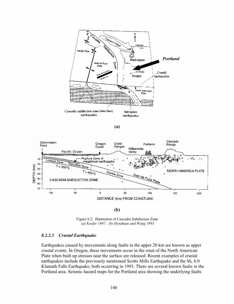
(a)

(b)

Figure 8.2: Illustration of Cascadia Subduction Zone (a) Keefer 1997; (b) Hyndman and Wang 1993

8.2.2.3 Crustal Earthquake

Earthquakes caused by movements along faults in the upper 20 kcrustal events. In Oregon, these movements occur in the crust of Plate when built up stresses near the surface are released. Recentearthquakes include the previously mentioned Scotts Mills EarthKlamath Falls Earthquake, both occurring in 1993. There are sevPortland area. Seismic hazard maps for the Portland area showing

146

Portland

m are known as upper the North American examples of crustal quake and the ML 6.0 eral known faults in the the underlying faults

have been recently developed (Wong et al. 2000). The three main faults around Portland are the Oatfield, Portland Hills, and East Bank Faults (shown in Figure 8.3). The East Bank Fault was used as the design fault in this study because of its close proximity to the site (8 km).

8.2.2.4 Probabilistic Assessment of Bedrock Ground Motions

Probabilistic uniform hazard studies have been completed for the Portland area in recent years that provide estimates of the peak ground acceleration values on rock (Geomatrix 1995; USGS 1999). These studies incorporate the relative contributions of the three seismic sources in the Portland area to develop one peak ground acceleration value for specified probabilities of exceedance in given time periods. Typically, values are estimated for earthquakes with a 10% probability of exceedance in 50 years and a 2% probability of exceedance in 50 years, which correspond to return periods of 475 and 2475 years, respectively. Figure 8.4 provides the PGA contours on bedrock with a 475-year return period as estimated by Geomatrix (1995).

SITE LOCATION

Figure 8.3: Portland Area Faults (Wong et al. 2000)

147

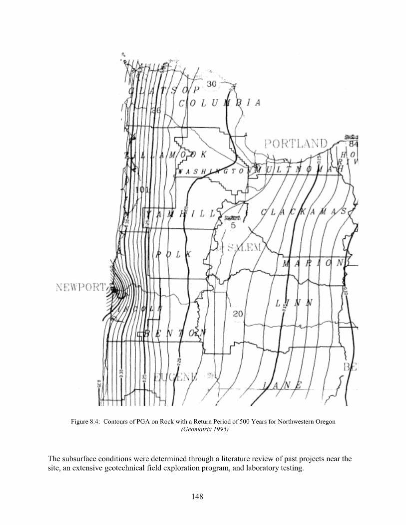
Figure 8.4: Contours of PGA on Rock with a Return Period of 500 Years for Northwestern Oregon (Geomatrix 1995)

The subsurface conditions were determined through a literature review of past projects near the site, an extensive geotechnical field exploration program, and laboratory testing.

148

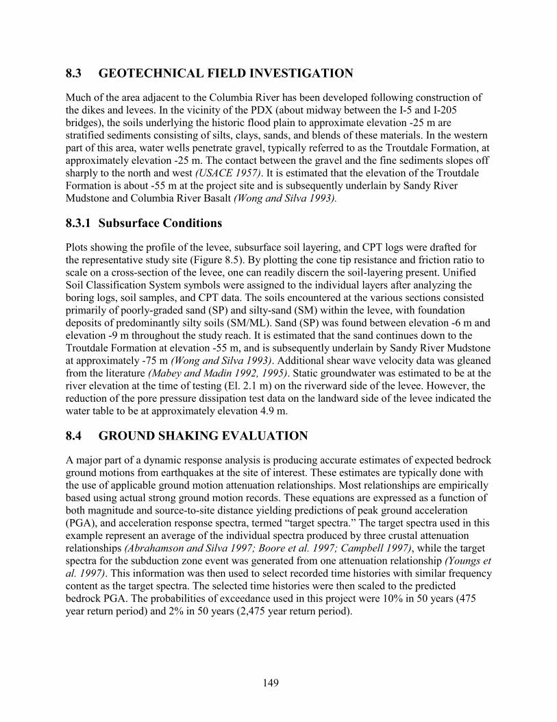
8.3 GEOTECHNICAL FIELD INVESTIGATION

Much of the area adjacent to the Columbia River has been developed following construction of the dikes and levees. In the vicinity of the PDX (about midway between the I-5 and I-205 bridges), the soils underlying the historic flood plain to approximate elevation -25 m are stratified sediments consisting of silts, clays, sands, and blends of these materials. In the western part of this area, water wells penetrate gravel, typically referred to as the Troutdale Formation, at approximately elevation -25 m. The contact between the gravel and the fine sediments slopes off sharply to the north and west (USACE 1957). It is estimated that the elevation of the Troutdale Formation is about -55 m at the project site and is subsequently underlain by Sandy River Mudstone and Columbia River Basalt (Wong and Silva 1993).

8.3.1 Subsurface Conditions

Plots showing the profile of the levee, subsurface soil layering, and CPT logs were drafted for the representative study site (Figure 8.5). By plotting the cone tip resistance and friction ratio to scale on a cross-section of the levee, one can readily discern the soil-layering present. Unified Soil Classification System symbols were assigned to the individual layers after analyzing the boring logs, soil samples, and CPT data. The soils encountered at the various sections consisted primarily of poorly-graded sand (SP) and silty-sand (SM) within the levee, with foundation deposits of predominantly silty soils (SM/ML). Sand (SP) was found between elevation -6 m and elevation -9 m throughout the study reach. It is estimated that the sand continues down to the Troutdale Formation at elevation -55 m, and is subsequently underlain by Sandy River Mudstone at approximately -75 m (Wong and Silva 1993). Additional shear wave velocity data was gleaned from the literature (Mabey and Madin 1992, 1995). Static groundwater was estimated to be at the river elevation at the time of testing (El. 2.1 m) on the riverward side of the levee. However, the reduction of the pore pressure dissipation test data on the landward side of the levee indicated the water table to be at approximately elevation 4.9 m.

8.4 GROUND SHAKING EVALUATION

A major part of a dynamic response analysis is producing accurate estimates of expected bedrock ground motions from earthquakes at the site of interest. These estimates are typically done with the use of applicable ground motion attenuation relationships. Most relationships are empirically based using actual strong ground motion records. These equations are expressed as a function of both magnitude and source-to-site distance yielding predictions of peak ground acceleration (PGA), and acceleration response spectra, termed “target spectra.” The target spectra used in this example represent an average of the individual spectra produced by three crustal attenuation relationships (Abrahamson and Silva 1997; Boore et al. 1997; Campbell 1997), while the target spectra for the subduction zone event was generated from one attenuation relationship (Youngs et al. 1997). This information was then used to select recorded time histories with similar frequency content as the target spectra. The selected time histories were then scaled to the predicted bedrock PGA. The probabilities of exceedance used in this project were 10% in 50 years (475 year return period) and 2% in 50 years (2,475 year return period).

149

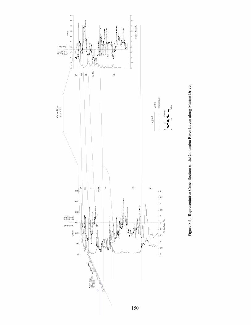
150

Fenceline

CPT Hole 4E26.0' NGVD

Borehole 4E

SP SM CL

ML

SP SM CL

ML

SPSP

Wat

er's

Edg

e2:

00 p

m 1

0/5/

997.

0' N

GV

D

42.4

' NG

VD

Mar

ine

Driv

e

Rip

Rap

(NTS

)

CPT Hole 4A 32.0' NGVD

Qc

(tsf)

Fric

tion

Rat

io

Lege

nd

010

02

20 f

eet

4 m

eter

s

SM-M

L

Qc

(tsf)

Qc

(tsf)

Fric

tion

Rat

io (%

)

Fric

tion

Rat

io (%

)

0

50

100

150

200

250

300

0

0.5

1

1.5

2

2.5

3

3.5

4

4.5

5

0

50

100

150

200

250

300

350

400

450

500

0

0.5

1

1.5

2

2.5

3

3.5

4

4.5

5

SM-M

LSP

Fi

gure

8.5

: R

epre

sent

ativ

e C

ross

-Sec

tion

of th

e C

olum

bia

Riv

er L

evee

alo

ng M

arin

e D

rive

Attenuation relationships were used to predict both PGA and spectral acceleration response content of each type of earthquake. Once the PGA and spectral response of the ground motions were determined, time history records of like events were selected for use in the dynamic ground response analysis. An effort was made to match distance, magnitude, spectral content and PGA for all input time histories with those of the predicted values, though the inherent variability in earthquakes motions do not allow for complete agreement with the smoothed spectra provided from the regression analyses on which the attenuation relationships are based.

8.4.1 Summary of Recent Seismic Hazard Investigations

Comparisons were made between the recommendations of the PGA on soil and rock from the following sources: (1) the Geomatrix (1995) report to the ODOT titled, Seismic Design Mapping of the State of Oregon, (2) the USGS’s National Seismic Mapping Project (USGS 2000), and (3) the URS Greiner/Woodward Clyde Portland Microzonation Maps (Wong et al. 2000). These recommendations are based on probabilistic, uniform hazard studies that combined the ground shaking contributions from the interplate, intraplate, and crustal earthquake scenarios, respectively, into one peak ground acceleration value for a given return period (Table 8.3). It should be noted that investigations by Geomatrix and the USGS provide recommendations for PGA on bedrock. The URS Greiner/Woodward Clyde report yields PGA values at the soil surface. The recommendations put forth in the URS Greiner/Woodward Clyde report, specifically the Portland area fault map shown in Figure 8.3, were incorporated into this demonstration application for the sake of completeness.

Table 8.3: Comparison of Recommended PGA Values for the Site GROUND MOTIONS ASSOCIATED WITH SPECIFIED

PROBABILITIES OF EXCEEDANCE PGAROCK PGAsoil

SOURCE 10% in 50 Years 2% in 50 Years 10% in 50 Years 2% in 50 Years USGS 0.19g 0.38g N/A N/A Geomatrix 0.19g 0.37g N/A N/A URS Greiner / Woodward Clyde N/A N/A 0.20g – 0.25g 0.40g

The peak ground accelerations provided by the seismic hazard studies referenced here reflect the contributions of all seismic sources in the region. These investigations yield uniform hazard data in that the value of peak horizontal acceleration for a given exposure time represents the combined, or “aggregate” hazard. The acceleration values cannot be directly attributed to a single source zone or single earthquake of given magnitude. For many seismic analyses in geotechnical and structural engineering, the earthquake magnitude is requisite input data. This is particularly important for analysis methods that incorporate the duration of ground motions, the number of significant cycles of shaking, or seismic energy. Soil liquefaction can be thought of as a fatigue failure of soils; therefore, the intensity of the shaking and number of loading cycles are necessary parameters in hazard evaluation. In order to use the acceleration values from hazard studies a de-aggregation of the hazard associated with individual seismic sources is required, to estimate the relative contribution of each seismic source and size of earthquake. This information is available for the seismic hazard studies presented by Geomatrix and the USGS.

151

8.4.2 Subduction Zone Bedrock Motions

Ground motion characteristics were estimated for Mw 8.5 and Mw 9.0 subduction zone earthquakes with a source-to-site distance of 85 km. The Mw 8.5 earthquake was chosen based on the recommendations published by Geomatrix (1995), and the Mw 9.0 was recommended by Wong et al. (2000). The PGArock was 0.12g and 0.14g for the Mw 8.5 and Mw 9.0 earthquakes, respectively, using an attenuation relationship created by Youngs et al. (1997). Recorded time histories from the Mw 8.5, 1985 Michoacán earthquake (Aeropuerto station) and the Mw 8.5, 1978 Miyagi-Oki (Ofunato station) subduction zone earthquakes were compared against the predicted target spectra, as shown in Figures 8.6 and 8.7.

Durations were on the order of 60-70 seconds. The selected records provide a satisfactory match of spectral content and were used as the design input bedrock ground motions for the dynamic ground motion analysis, after scaling to the appropriate PGArock values of 0.12g and 0.14g. The predicted earthquake parameters are shown in Table 8.4 and the selected time history data is shown in Table 8.5. The intraplate earthquake was not considered in the analyses because the interplate and crustal earthquake scenarios would sufficiently “bracket” the seismic hazard.

(5% Damping)

0.00

0.10

0.20

0.30

0.40

0.50

0.60

0.70

0.80

0.90

1.00

1.10

1.20

1.30

1.40

1.50

0 0.5 1 1.5 2 2.5 3Period (sec)

Spec

tral

Acc

eler

atio

n (g

)

Magnitude 8.5 Target Spectrum

Scaled Aeropuerto Ground Motion

Scaled Ofunato Ground Motion

Figure 8.6: Aeropuerto and Ofunato (Scaled PGA = 0.12g) Response Spectra Compared to the Magnitude 8.5 Cascadia Subduction Zone Target Spectrum on Rock

152

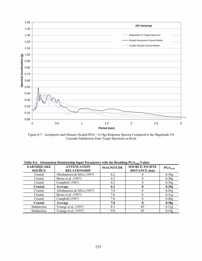
(5% Damping)

0.00

0.10

0.20

0.30

0.40

0.50

0.60

0.70

0.80

0.90

1.00

1.10

1.20

1.30

1.40

1.50

0 0.5 1 1.5 2 2.5Period (sec)

Spec

tral

Acc

eler

atio

n (g

)

3

Magnitude 9.0 Target Spectrum

Scaled Aeropuerto Ground Motion

Scaled Ofunato Ground Motion

Figure 8.7: Aeropuerto and Ofunato (Scaled PGA = 0.14g) Response Spectra Compared to the Magnitude 9.0

Cascadia Subduction Zone Target Spectrum on Rock

Table 8.4: Attenuation Relationship Input Parameters with the Resulting PGArock Values EARTHQUAKE

SOURCE ATTENUATION RELATIONSHIP

MAGNITUDE SOURCE-TO-SITE DISTANCE (km)

PGArock

Crustal Abrahamson & Silva (1997) 6.2 8 0.30g Crustal Boore et al. (1997) 6.2 8 0.20g Crustal Campbell (1997) 6.2 8 0.36g Crustal Average 6.2 8 0.29g Crustal Abrahamson & Silva (1997) 7.0 8 0.45g Crustal Boore et al. (1997) 7.0 8 0.31g Crustal Campbell (1997) 7.0 8 0.40g Crustal Average 7.0 8 0.38g

Subduction Youngs et al. (1997) 8.5 85 0.12g Subduction Youngs et al. (1997) 9.0 85 0.14g

153

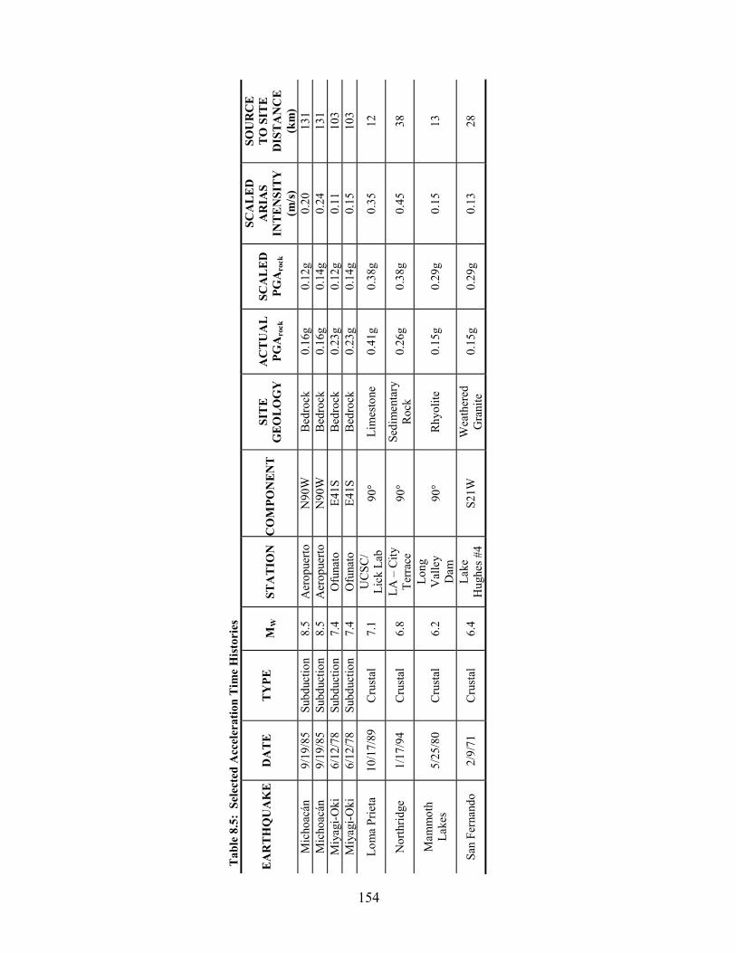
154

Tab

le 8

.5:

Sele

cted

Acc

eler

atio

n T

ime

His

tori

es

EA

RT

HQ

UA

KE

DA

TE

TY

PEM

W

STA

TIO

NC

OM

PON

EN

TSI

TE

G

EO

LO

GY

A

CT

UA

L

PGA

rock

SCA

LE

D

PGA

rock

SCA

LE

D

AR

IAS

INT

EN

SIT

Y

(m/s

)

SOU

RC

E

TO

SIT

E

DIS

TA

NC

E

(km

) M

icho

acán

9/

19/8

5Su

bduc

tion

8.5

Aer

opue

rtoN

90W

Bed

rock

0.16

g0.

12g

0.20

131

Mic

hoac

án

9/19

/85

Subd

uctio

n8.

5A

erop

uerto

N90

WB

edro

ck0.

16g

0.14

g0.

2413

1M

iyag

i-Oki

6/

12/7

8Su

bduc

tion

7.4

Ofu

nato

E41S

Bed

rock

0.23

g0.

12g

0.11

103

Miy

agi-O

ki

6/12

/78

Subd

uctio

n7.

4O

funa

toE4

1SB

edro

ck0.

23g

0.14

g0.

1510

3

Lom

a Pr

ieta

10

/17/

89

Cru

stal

7.

1 U

CSC

/ Li

ck L

ab

90�

Lim

esto

ne

0.41

g0.

38g

0.35

12

Nor

thrid

ge

1/

17/9

4C

rust

al6.

8LA

– C

ity

Terr

ace

90�

Sedi

men

tary

R

ock

0.26

g0.

38g

0.45

38

Mam

mot

h La

kes

5/25

/80

C

rust

al6.

2Lo

ng

Val

ley

Dam

90

�

Rhy

olite

0.15

g0.

29g

0.15

13

San

Fern

ando

2/

9/71

C

rust

al

6.4

Lake

H

ughe

s #4

S21W

W

eath

ered

G

rani

te

0.15

g

0.29

g0.

1328

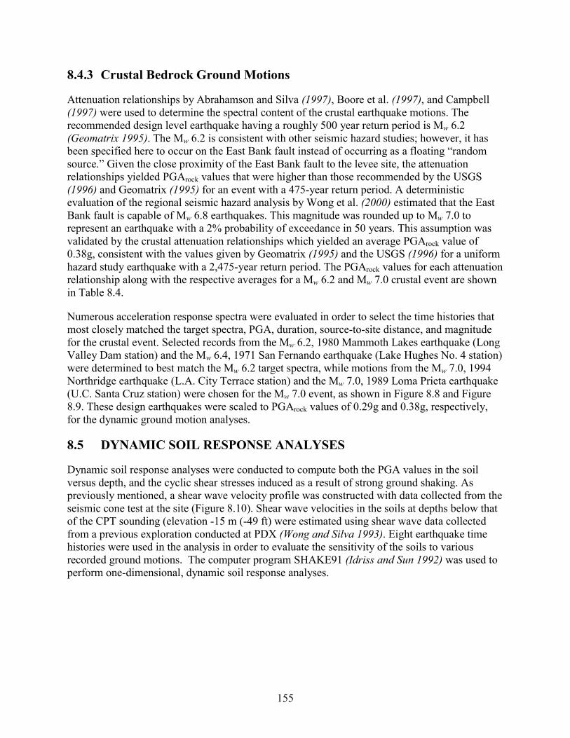
8.4.3 Crustal Bedrock Ground Motions

Attenuation relationships by Abrahamson and Silva (1997), Boore et al. (1997), and Campbell (1997) were used to determine the spectral content of the crustal earthquake motions. The recommended design level earthquake having a roughly 500 year return period is Mw 6.2 (Geomatrix 1995). The Mw 6.2 is consistent with other seismic hazard studies; however, it has been specified here to occur on the East Bank fault instead of occurring as a floating “random source.” Given the close proximity of the East Bank fault to the levee site, the attenuation relationships yielded PGArock values that were higher than those recommended by the USGS (1996) and Geomatrix (1995) for an event with a 475-year return period. A deterministic evaluation of the regional seismic hazard analysis by Wong et al. (2000) estimated that the East Bank fault is capable of Mw 6.8 earthquakes. This magnitude was rounded up to Mw 7.0 to represent an earthquake with a 2% probability of exceedance in 50 years. This assumption was validated by the crustal attenuation relationships which yielded an average PGArock value of 0.38g, consistent with the values given by Geomatrix (1995) and the USGS (1996) for a uniform hazard study earthquake with a 2,475-year return period. The PGArock values for each attenuation relationship along with the respective averages for a Mw 6.2 and Mw 7.0 crustal event are shown in Table 8.4.

Numerous acceleration response spectra were evaluated in order to select the time histories that most closely matched the target spectra, PGA, duration, source-to-site distance, and magnitude for the crustal event. Selected records from the Mw 6.2, 1980 Mammoth Lakes earthquake (Long Valley Dam station) and the Mw 6.4, 1971 San Fernando earthquake (Lake Hughes No. 4 station) were determined to best match the Mw 6.2 target spectra, while motions from the Mw 7.0, 1994 Northridge earthquake (L.A. City Terrace station) and the Mw 7.0, 1989 Loma Prieta earthquake (U.C. Santa Cruz station) were chosen for the Mw 7.0 event, as shown in Figure 8.8 and Figure 8.9. These design earthquakes were scaled to PGArock values of 0.29g and 0.38g, respectively, for the dynamic ground motion analyses.

8.5 DYNAMIC SOIL RESPONSE ANALYSES

Dynamic soil response analyses were conducted to compute both the PGA values in the soil versus depth, and the cyclic shear stresses induced as a result of strong ground shaking. As previously mentioned, a shear wave velocity profile was constructed with data collected from the seismic cone test at the site (Figure 8.10). Shear wave velocities in the soils at depths below that of the CPT sounding (elevation -15 m (-49 ft) were estimated using shear wave data collected from a previous exploration conducted at PDX (Wong and Silva 1993). Eight earthquake time histories were used in the analysis in order to evaluate the sensitivity of the soils to various recorded ground motions. The computer program SHAKE91 (Idriss and Sun 1992) was used to perform one-dimensional, dynamic soil response analyses.

155

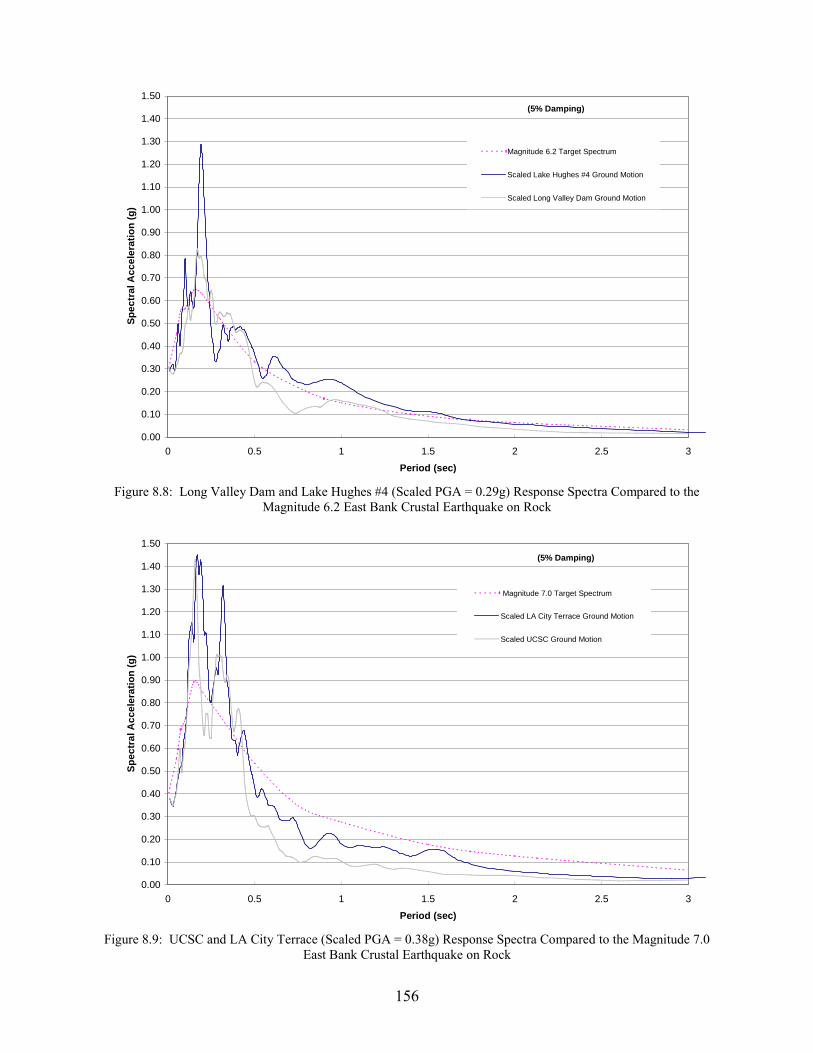
(5% Damping)

0.00

0.10

0.20

0.30

0.40

0.50

0.60

0.70

0.80

0.90

1.00

1.10

1.20

1.30

1.40

1.50

0 0.5 1 1.5 2 2.5Period (sec)

Spec

tral

Acc

eler

atio

n (g

)

3

Magnitude 6.2 Target Spectrum

Scaled Lake Hughes #4 Ground Motion

Scaled Long Valley Dam Ground Motion

Figure 8.8: Long Valley Dam and Lake Hughes #4 (Scaled PGA = 0.29g) Response Spectra Compared to the

Magnitude 6.2 East Bank Crustal Earthquake on Rock

(5% Damping)

0.00

0.10

0.20

0.30

0.40

0.50

0.60

0.70

0.80

0.90

1.00

1.10

1.20

1.30

1.40

1.50

0 0.5 1 1.5 2 2.5Period (sec)

Spec

tral

Acc

eler

atio

n (g

)

3

Magnitude 7.0 Target Spectrum

Scaled LA City Terrace Ground Motion

Scaled UCSC Ground Motion

Figure 8.9: UCSC and LA City Terrace (Scaled PGA = 0.38g) Response Spectra Compared to the Magnitude 7.0

East Bank Crustal Earthquake on Rock

156

-100.0

-90.0

-80.0

-70.0

-60.0

-50.0

-40.0

-30.0

-20.0

-10.0

0.0

10.0

0 200 400 600 800 1000 1200 1400 1600

Shear Wave Velocity, Vs (m/sec)

Ele

vatio

n (m

)Foundation Soils (SM/ML)

Sand

Troutdale Gravels

Sandy River Mudstone

157

Figure 8.10: Shear Wave Velocity Profile at Location 4E

8.5.1 Dynamic Response Analysis Method, SHAKE91

The SHAKE91 program (Idriss and Sun 1992) was used to compute the response of the subsurface to vertically propagating shear waves. The program assumes the subsurface consists of visco-elastic, isotropic, and homogeneous material (soil) of infinite horizontal extent. Each layer is also assumed to be completely described by shear modulus (G), damping ratio (�)��total unit weight (�), and layer thickness (h). The continuous solution to the wave equation is the basis for SHAKE91. The wave equation is adapted for use with transient motion through the use of the Fast Fourier Transform algorithm. Because the analysis uses the Fast Fourier Transform, and therefore, the frequency domain, it is a linear analysis. However, G and � are nonlinear, strain-dependent soil properties. The nonlinearity of these properties is accounted for by using an iterative, equivalent nonlinear procedure to find strain compatible modulus and damping ratios

with the calculated equivalent uniform strain, in each layer, from user defined modulus reduction and damping curves. Plasticity Index dependent curves developed by Vucetic and Dobry (1991) and confining stress dependent curves developed by Seed et al. (1984) were used to model modulus and damping ratio for cohesive and cohesionless soils, respectively. The modulus reduction and soil damping curves used in this study are shown in Figures 8.11 and 8.12.

Figure 8.11: Variation of G/Gmax versus Cyclic Shear Strain as a Function of Soil Plasticity for Normally and Overconsolidated Soils (after Vucetic and Dobry 1991)

158

Figure 8.12: Variation of G/Gmax versus λ versus Cyclic Shear Strain for Cohesionless Soils (after Seed et al. 1984)

The SHAKE91 program utilizes initial estimates of modulus and damping ratio to calculate a maximum shear strain in each layer. This maximum strain is multiplied by a reduction factor, (n), to produce an average strain, or equivalent uniform strain, in each layer. The value of (n), defined as the ratio of the equivalent uniform strain divided by the maximum calculated strain, is typically set between 0.40 to 0.75 depending on the characteristics of the bedrock input motion, or simply as a function of the magnitude of earthquake motions being modeled. The following equation has been recommended to estimate this ratio (Idriss and Sun 1992):

159

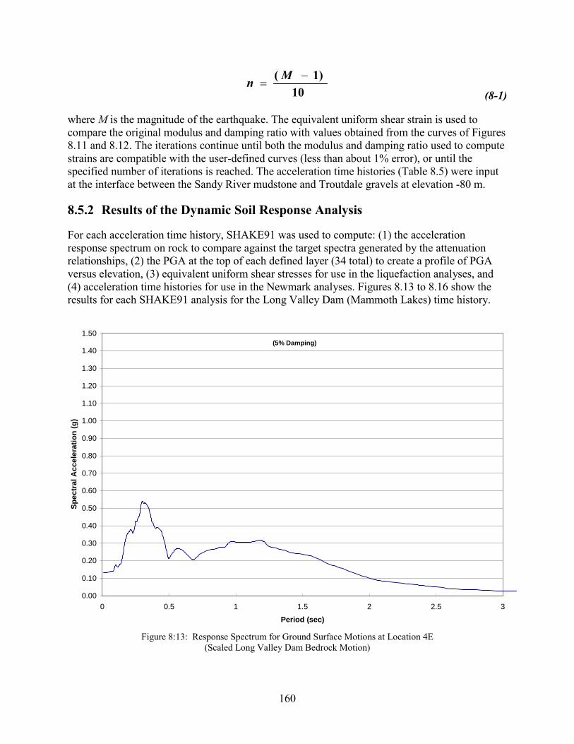
101)( �

�

Mn (8-1)

where M is the magnitude of the earthquake. The equivalent uniform shear strain is used to compare the original modulus and damping ratio with values obtained from the curves of Figures 8.11 and 8.12. The iterations continue until both the modulus and damping ratio used to compute strains are compatible with the user-defined curves (less than about 1% error), or until the specified number of iterations is reached. The acceleration time histories (Table 8.5) were input at the interface between the Sandy River mudstone and Troutdale gravels at elevation -80 m.

8.5.2 Results of the Dynamic Soil Response Analysis

For each acceleration time history, SHAKE91 was used to compute: (1) the acceleration response spectrum on rock to compare against the target spectra generated by the attenuation relationships, (2) the PGA at the top of each defined layer (34 total) to create a profile of PGA versus elevation, (3) equivalent uniform shear stresses for use in the liquefaction analyses, and (4) acceleration time histories for use in the Newmark analyses. Figures 8.13 to 8.16 show the results for each SHAKE91 analysis for the Long Valley Dam (Mammoth Lakes) time history.

(5% Damping)

0.00

0.10

0.20

0.30

0.40

0.50

0.60

0.70

0.80

0.90

1.00

1.10

1.20

1.30

1.40

1.50

0 0.5 1 1.5 2 2.5

Period (sec)

Spec

tral

Acc

eler

atio

n (g

)

3

Figure 8:13: Response Spectrum for Ground Surface Motions at Location 4E

(Scaled Long Valley Dam Bedrock Motion)

160

161

-90

-80

-70

-60

-50

-40

-30

-20

-1001020

00.

10.

20.

30.

4PG

A (g

)

Elevation (m)

PGA

= 0.

29g

at B

edro

ck

-90

-80

-70

-60

-50

-40

-30

-20

-1001020

020

4060

80

�eq

. Uni

form

(kPa

)Elevation (m)

Figu

re 8

.15:

Equ

ival

ent U

nifo

rm S

hear

Stre

ss P

rofil

e fo

r Sca

led

Lon

g V

alle

y D

am B

edro

ck M

otio

n at

Loc

atio

n 4E

Fi

gure

8.1

4: C

ompu

ted

Prof

ile o

f Pea

k G

roun

d A

ccel

erat

ion

for

Scal

ed L

ong

Val

ley

Dam

Bed

rock

Mot

ion

at L

ocat

ion

4E

-0.20

-0.15

-0.10

-0.05

0.00

0.05

0.10

0.15

0.20

0 5 10 15 20 25

Time (sec)

Acc

eler

atio

n (g

)

a) Elevation 6.4 m (21 ft)

-0.20

-0.15

-0.10

-0.05

0.00

0.05

0.10

0.15

0.20

0 5 10 15 20 25

Time (sec)

Acc

eler

atio

n (g

)

b) Elevation 1.5 m (5 ft)

Figure 8.16: Time Histories Computed for Scaled Long Valley Dam Bedrock Motion at Location 4E

The profiles of PGA versus elevation show significant damping of the PGA values for the crustal events. There was an approximate 50% reduction in the PGArock when compared to the PGAsoil at the top of the levee. Table 8.6 summarizes the PGArock and computed PGAsoil values.

162

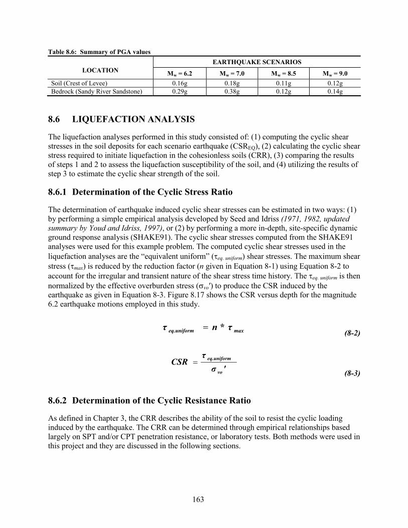
Table 8.6: Summary of PGA values EARTHQUAKE SCENARIOS

LOCATION Mw = 6.2 Mw = 7.0 Mw = 8.5 Mw = 9.0 Soil (Crest of Levee) 0.16g 0.18g 0.11g 0.12g Bedrock (Sandy River Sandstone) 0.29g 0.38g 0.12g 0.14g

8.6 LIQUEFACTION ANALYSIS

The liquefaction analyses performed in this study consisted of: (1) computing the cyclic shear stresses in the soil deposits for each scenario earthquake (CSREQ), (2) calculating the cyclic shear stress required to initiate liquefaction in the cohesionless soils (CRR), (3) comparing the results of steps 1 and 2 to assess the liquefaction susceptibility of the soil, and (4) utilizing the results of step 3 to estimate the cyclic shear strength of the soil.

8.6.1 Determination of the Cyclic Stress Ratio

The determination of earthquake induced cyclic shear stresses can be estimated in two ways: (1) by performing a simple empirical analysis developed by Seed and Idriss (1971, 1982, updated summary by Youd and Idriss, 1997), or (2) by performing a more in-depth, site-specific dynamic ground response analysis (SHAKE91). The cyclic shear stresses computed from the SHAKE91 analyses were used for this example problem. The computed cyclic shear stresses used in the liquefaction analyses are the “equivalent uniform” (�eq. uniform) shear stresses. The maximum shear stress (�max) is reduced by the reduction factor (n given in Equation 8-1) using Equation 8-2 to account for the irregular and transient nature of the shear stress time history. The �eq. uniform is then normalized by the effective overburden stress (�vo′) to produce the CSR induced by the earthquake as given in Equation 8-3. Figure 8.17 shows the CSR versus depth for the magnitude 6.2 earthquake motions employed in this study.

(8-2) maxeq.uniform τ*nτ �

'στ

CSRvo

eq.uniform�

(8-3)

8.6.2 Determination of the Cyclic Resistance Ratio

As defined in Chapter 3, the CRR describes the ability of the soil to resist the cyclic loading induced by the earthquake. The CRR can be determined through empirical relationships based largely on SPT and/or CPT penetration resistance, or laboratory tests. Both methods were used in this project and they are discussed in the following sections.

163

-15.0

-12.5

-10.0

-7.5

-5.0

-2.5

0.0

2.5

5.0

7.5

10.0

12.5

15.0

0.00 0.02 0.04 0.06 0.08 0.10 0.12 0.14Cyclic Stress Ratio, CSR

Elev

atio

n (m

)

Long Valley Dam

Lake Hughes #4

Figure 8.17: Cyclic Stress Ratio Profile for the Magnitude 6.2 Earthquakes

8.6.2.1 Laboratory Tests

Cyclic triaxial tests were performed to determine the cyclic behavior of the silty and fine sandy soils at the site. Undrained, stress-controlled tests consisting of uniform sinusoidal loading were carried out at a frequency of 1 Hz. The cyclic loads were applied to the specimens until: (1) a single amplitude axial strain of 5% was reached, or (2) 100 loading cycles, whichever occurred first. The limiting axial strain of 5% was selected in order to preserve the shape of the specimen for the post-cyclic load tests. The CRR values obtained from the laboratory tests was corrected to field CRR values through the use of correction factors (Chapter 3).

The results of the cyclic triaxial tests on silty soils are presented in Table 3.8 and Figure 3.11. Cyclic triaxial tests conducted on soils from the Columbia River levee adjacent to PDX and from Hayden Island are presented to further illustrate the expected shape of the cyclic resistance curves. The laboratory results demonstrated an increase in the cyclic resistance ratio with increasing overconsolidation ratio (OCR). However, the silts were

164

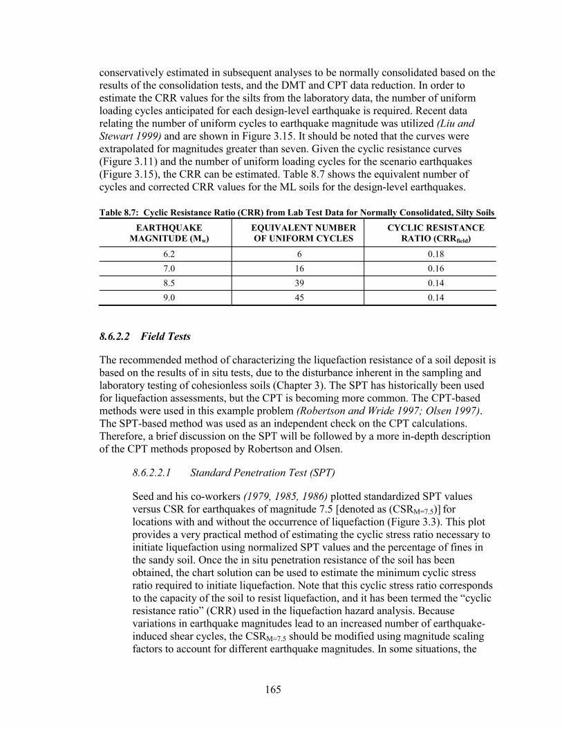
conservatively estimated in subsequent analyses to be normally consolidated based on the results of the consolidation tests, and the DMT and CPT data reduction. In order to estimate the CRR values for the silts from the laboratory data, the number of uniform loading cycles anticipated for each design-level earthquake is required. Recent data relating the number of uniform cycles to earthquake magnitude was utilized (Liu and Stewart 1999) and are shown in Figure 3.15. It should be noted that the curves were extrapolated for magnitudes greater than seven. Given the cyclic resistance curves (Figure 3.11) and the number of uniform loading cycles for the scenario earthquakes (Figure 3.15), the CRR can be estimated. Table 8.7 shows the equivalent number of cycles and corrected CRR values for the ML soils for the design-level earthquakes.

Table 8.7: Cyclic Resistance Ratio (CRR) from Lab Test Data for Normally Consolidated, Silty Soils

EARTHQUAKE MAGNITUDE (Mw)

EQUIVALENT NUMBER OF UNIFORM CYCLES

CYCLIC RESISTANCE RATIO (CRRfield)

6.2 6 0.18 7.0 16 0.16 8.5 39 0.14 9.0 45 0.14

8.6.2.2 Field Tests

The recommended method of characterizing the liquefaction resistance of a soil deposit is based on the results of in situ tests, due to the disturbance inherent in the sampling and laboratory testing of cohesionless soils (Chapter 3). The SPT has historically been used for liquefaction assessments, but the CPT is becoming more common. The CPT-based methods were used in this example problem (Robertson and Wride 1997; Olsen 1997). The SPT-based method was used as an independent check on the CPT calculations. Therefore, a brief discussion on the SPT will be followed by a more in-depth description of the CPT methods proposed by Robertson and Olsen.

8.6.2.2.1 Standard Penetration Test (SPT)

Seed and his co-workers (1979, 1985, 1986) plotted standardized SPT values versus CSR for earthquakes of magnitude 7.5 [denoted as (CSRM=7.5)] for locations with and without the occurrence of liquefaction (Figure 3.3). This plot provides a very practical method of estimating the cyclic stress ratio necessary to initiate liquefaction using normalized SPT values and the percentage of fines in the sandy soil. Once the in situ penetration resistance of the soil has been obtained, the chart solution can be used to estimate the minimum cyclic stress ratio required to initiate liquefaction. Note that this cyclic stress ratio corresponds to the capacity of the soil to resist liquefaction, and it has been termed the “cyclic resistance ratio” (CRR) used in the liquefaction hazard analysis. Because variations in earthquake magnitudes lead to an increased number of earthquake-induced shear cycles, the CSRM=7.5 should be modified using magnitude scaling factors to account for different earthquake magnitudes. In some situations, the

165

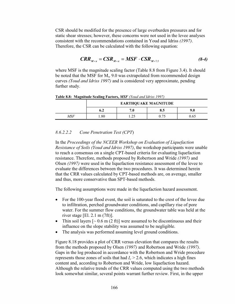
CSR should be modified for the presence of large overburden pressures and for static shear stresses; however, these concerns were not used in the levee analyses consistent with the recommendations contained in Youd and Idriss (1997). Therefore, the CSR can be calculated with the following equation:

(8-4) 57.MxMxM CSRMSFCSRCRR���

���

where MSF is the magnitude scaling factor (Table 8.8 from Figure 3.4). It should be noted that the MSF for Mw 9.0 was extrapolated from recommended design curves (Youd and Idriss 1997) and is considered very approximate, pending further study.

Table 8.8: Magnitude Scaling Factors, MSF (Youd and Idriss 1997)

EARTHQUAKE MAGNITUDE

6.2 7.0 8.5 9.0 MSF 1.80 1.25 0.75 0.65

8.6.2.2.2 Cone Penetration Test (CPT)

In the Proceedings of the NCEER Workshop on Evaluation of Liquefaction Resistance of Soils (Youd and Idriss 1997), the workshop participants were unable to reach a consensus on a single CPT-based criteria for evaluating liquefaction resistance. Therefore, methods proposed by Robertson and Wride (1997) and Olsen (1997) were used in the liquefaction resistance assessment of the levee to evaluate the differences between the two procedures. It was determined herein that the CRR values calculated by CPT-based methods are, on average, smaller and thus, more conservative than SPT-based methods.

The following assumptions were made in the liquefaction hazard assessment.

� For the 100-year flood event, the soil is saturated to the crest of the levee due to infiltration, perched groundwater conditions, and capillary rise of pore water. For the summer flow conditions, the groundwater table was held at the river stage [El. 2.1 m (7ft)].

� Thin soil layers [~ 0.6 m (2 ft)] were assumed to be discontinuous and their influence on the slope stability was assumed to be negligible.

� The analysis was performed assuming level ground conditions.

Figure 8.18 provides a plot of CRR versus elevation that compares the results from the methods proposed by Olsen (1997) and Robertson and Wride (1997). Gaps in the log produced in accordance with the Robertson and Wride procedure represents those zones of soils that had Ic > 2.6, which indicates a high fines content and, according to Robertson and Wride, low liquefaction hazard. Although the relative trends of the CRR values computed using the two methods look somewhat similar, several points warrant further review. First, in the upper

166

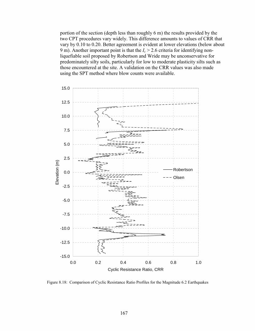
portion of the section (depth less than roughly 6 m) the results provided by the two CPT procedures vary widely. This difference amounts to values of CRR that vary by 0.10 to 0.20. Better agreement is evident at lower elevations (below about 9 m). Another important point is that the Ic > 2.6 criteria for identifying non-liquefiable soil proposed by Robertson and Wride may be unconservative for predominately silty soils, particularly for low to moderate plasticity silts such as those encountered at the site. A validation on the CRR values was also made using the SPT method where blow counts were available.

-15.0

-12.5

-10.0

-7.5

-5.0

-2.5

0.0

2.5

5.0

7.5

10.0

12.5

15.0

0.0 0.2 0.4 0.6 0.8 1.0Cyclic Resistance Ratio, CRR

Elev

atio

n (m

)

Robertson

Olsen

Figure 8.18: Comparison of Cyclic Resistance Ratio Profiles for the Magnitude 6.2 Earthquakes

167

8.7 EVALUATION OF INITIATION OF LIQUEFACTION

After the CSR caused by the earthquake and the CRR were determined, the potential for liquefaction was evaluated. At elevations where the CSR is greater than the CRR, liquefaction is likely to occur. The factor of safety against liquefaction (FSL) was evaluated at specific depths with the Equation 8-5. The CRR values used in the FSL calculations were from the CPT-based evaluation proposed by Robertson and Wride (1997) for sandy soils (SP/SM), and the laboratory cyclic triaxial cell testing on the fine-grained (ML) soils. Profiles of FSL as a function of elevation for each scenario earthquake were completed (Figure 8.19). A cross-section showing zones of soil that are expected to liquefy (FSL < 1.0), and zones expected to have significant excess pore pressure generation (1.0 < FSL < 1.4) during the Mw 8.5 earthquake is shown in Figure 8.20.

CSRCRRFSl �

(8-5)

8.8 DETERMINATION OF CYCLIC SHEAR STRENGTH

In order to assess the seismic stability of the levee, it was necessary to estimate the residual shear strength of the soils prone to excess pore pressure generation. The loss of soil shear strength is a function of the magnitude of excess pore pressure generation. The following categories delineate the various stages of soil shear strength reduction due to liquefaction.

� FSL > 1.4: Excess pore pressure generation is considered negligible and the soil does not experience an appreciable reduction in shear strength (CDMG 1997). In this case, the drained shear strength is computed using the standard Mohr-Coulomb strength equation.

� 1.0 < FSL < 1.4: Partial excess pore pressure generation will have an effect on soil strength and should be addressed. The magnitude of the pore pressure generation is a function of FSL and soil type (Marcuson et al. 1990).

� FSL < 1.0: Soils are expected to experience full pore pressure generation and residual shear strengths should be applied (Seed and Harder 1990; Stark and Mesri 1992; Ishihara 1993; Baziar and Dobry 1995).

8.8.1 Partial Excess Pore Pressure Generation (1.0 < FSL <1.4)

The relationship between the excess pore pressure ratio (ru) and the factor of safety against liquefaction for both gravel and sand is shown in (Figure 3.18). The excess pore pressure ratio is the relationship between the residual excess pore pressure (uexcess) and the effective overburden pressure (�′vo) given by:

vo

excess

σ'u

ru�

(8-6)

168

-15.0

-12.5

-10.0

-7.5

-5.0

-2.5

0.0

2.5

5.0

7.5

10.0

12.5

15.0

0.0 1.0 2.0 3.0 4.0 5.0Factor of Safety

Elev

atio

n (m

)

Long Valley Dam

Lake Hughes #4

Fact

or o

f Saf

ety

= 1.

0

Fact

or o

f Saf

ety

= 1.

4

Figure 8.19: Factor of Safety against Liquefaction (FSL) Profiles for Magnitude 6.2 Earthquakes

169

170

Figu

re 8

.20:

Cro

ss-S

ectio

n Ill

ustra

ting

Laye

rs S

usce

ptib

le to

Liq

uefa

ctio

n fo

r Mag

nitu

de 8

.5 E

arth

quak

e

0042

.4' N

GM

arin

e D

rive

cres

t sta

geV

D42

.5 ft

NG

VD

10

0 yr

floo

d st

age

28.9

ft N

GV

DSP SM

Rip

Rap

(NTS

)SM

CL

low

stag

e SM

-ML

7.0

ft N

GV

D

SP

SP

ML SP

Liqu

efac

tion

Lege

nd

1.0

< FS

FS >

1.4

4 met

ers

02

> 1

.41

20 fe

etFS

< 1

.0

The common method for reducing the static strength to account for partial pore pressure generation utilizes the Mohr-Coulomb shear strength equation for cohesionless soils (Equation 8-7). The vertical effective stress is initially calculated at the elevation of interest under hydrostatic conditions. The undrained strength is then calculated using a reduced vertical effective stress that accounts for the excess pore pressure generation (from ru) and using the static effective friction angle (�'static). Next, a reduced effective friction angle (�'equivalent) is back-calculated using the aforementioned undrained shear strength, the initial vertical effective stress, and �'static. Given this process, Equation 8-8 was derived directly relating �'equivalent to ru and �'static that is independent of the in situ vertical effective stress (Ebeling and Morrison 1993). Therefore, in soil layers that experience pore pressure generation, the static shear strength of the soil is reduced using a residual effective friction angle, as opposed to reducing the vertical effective stress. This modification is required because of the inability of standard slope stability computer programs to directly account for excess pore pressure generation.

(8-7) '�tannσ'τ �

(8-8) � �� staticuequivalent r' �� tan1arctan �� �

It was assumed that excess pore pressure generation was only significant when the soils had FSL < 1.4. To facilitate efficient spreadsheet analyses, ru was held constant at 0.4 for soils that had 1.0 < FSL < 1.4.

8.8.2 Liquefied State (FSL < 1)

The two general procedures used to estimate the residual undrained shear strength of the fully liquefied soils were: (1) residual strength ratio methods (Stark and Mesri 1992; Ishihara 1993; Baziar and Dobry 1995); and (2) a procedure that is independent of the in situ vertical effective stress (Seed and Harder 1990). The Stark and Mesri method was used exclusively here, although the other procedures referenced in Chapter 4 were used for validation purposes.

The relationship between the normalized clean sand blowcount value, (N1)60 CS, and the residual undrained critical strength ratio for magnitude 7.5 earthquakes developed by Stark and Mesri (1992) is illustrated in Figure 4.3. The yield strength curve provides undrained strengths that are most closely consistent with the results of the aforementioned work by Baziar and Dobry (1995) and Ishihara (1993); therefore this relationship (Equation 4-3) was used in this study.

It should be noted that the “clean sand” penetration resistance (N1)60 CS used in the residual undrained shear strength evaluation is not the same as the (N1)60 CS used in the liquefaction triggering analyses. The clean sand blow count (N1)60 CS is calculated using Equation 4-4 and the correction data provided in Table 4.1. At elevations where blowcount information was not available (Shelby tube sample locations), values were estimated from CPT data. The estimated fines content values for levee soils susceptible to liquefaction are listed in Table 8.9.

171

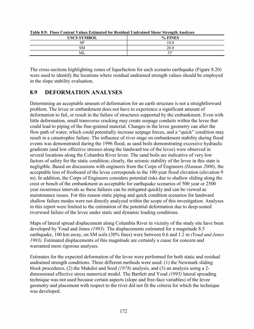
Table 8.9: Fines Content Values Estimated for Residual Undrained Shear Strength Analyses USCS SYMBOL % FINES

SP 10.0 SM 20.0 ML 35+

The cross-sections highlighting zones of liquefaction for each scenario earthquake (Figure 8.20) were used to identify the locations where residual undrained strength values should be employed in the slope stability evaluation.

8.9 DEFORMATION ANALYSES

Determining an acceptable amount of deformation for an earth structure is not a straightforward problem. The levee or embankment does not have to experience a significant amount of deformation to fail, or result in the failure of structures supported by the embankment. Even with little deformation, small transverse cracking may create seepage conduits within the levee that could lead to piping of the fine-grained material. Changes in the levee geometry can alter the flow path of water, which could potentially increase seepage forces, and a “quick” condition may result in a catastrophic failure. The influence of river stage on embankment stability during flood events was demonstrated during the 1996 flood, as sand boils demonstrating excessive hydraulic gradients (and low effective stresses along the landward toe of the levee) were observed in several locations along the Columbia River levee. The sand boils are indicative of very low factors of safety for the static condition; clearly, the seismic stability of the levee in this state is negligible. Based on discussions with engineers from the Corps of Engineers (Hannan 2000), the acceptable loss of freeboard of the levee corresponds to the 100-year flood elevation (elevation 9 m). In addition, the Corps of Engineers considers potential risks due to shallow sliding along the crest or bench of the embankment as acceptable for earthquake scenarios of 500 year or 2500 year recurrence intervals as these failures can be mitigated quickly and can be viewed as maintenance issues. For this reason static piping and quick condition scenarios for landward shallow failure modes were not directly analyzed within the scope of this investigation. Analyses in this report were limited to the estimation of the potential deformation due to deep-seated riverward failure of the levee under static and dynamic loading conditions.

Maps of lateral spread displacement along Columbia River in vicinity of the study site have been developed by Youd and Jones (1993). The displacements estimated for a magnitude 8.5 earthquake, 100 km away, on SM soils (30% fines) were between 0.6 and 1.2 m (Youd and Jones 1993). Estimated displacements of this magnitude are certainly a cause for concern and warranted more rigorous analyses.

Estimates for the expected deformation of the levee were performed for both static and residual undrained strength conditions. Three different methods were used: (1) the Newmark sliding block procedures, (2) the Makdisi and Seed (1978) analysis, and (3) an analysis using a 2-dimensional effective stress numerical model. The Bartlett and Youd (1995) lateral spreading technique was not used because certain aspects (slope and free-face variables) of the levee geometry and placement with respect to the river did not fit the criteria for which the technique was developed.

172

8.9.1 Newmark Sliding Block Analyses

Rigid body, sliding block analyses, which assume that the soil behaves as a rigid, perfectly plastic material, can be used to estimate limited earthquake-induced deformations (Chapter 4). The technique is based on a simple limit equilibrium stability analysis for determining the yield acceleration that is required to bring the factor of safety against sliding for a specified block of soil to unity.

In order to calculate the yield acceleration, ay, (Equation 8-9) of the slide mass, the values for the static factor of safety (FSstatic), the residual or post-liquefaction factor of safety (FSresidual), and the thrust angle (�) had to be determined. The values of FSstatic and FSresidual were calculated using the standard limit equilibrium methods found in the models UTEXAS3 and GeoSlope for deep-seated riverward failures at each design water level. The thrust angle for a circular failure is the angle between the vertical and a line drawn through the center of the failure circle to the center of gravity of the failure mass. A constant value of 10 degrees was used for the thrust angle of the estimated circular failures.

(8-9) �sin)1( ���� gFSa dualstaticresiy

The deformations induced by individual time histories are calculated by integrating the acceleration record twice over each period in which the acceleration exceeded ay to calculate the relative velocity and displacement. The total displacement of the sliding block is the summation of the incremental displacements. It should be noted that the Newmark analysis does not explicitly take into account continued movement due to inertial effects after acceleration values from the time histories drop below the critical acceleration. The simplest and most widely used method to account for the continued movement is to assume that the block decelerates at the same rate as it accelerates (Jibson 1993). This approach was adopted here.

The procedure also neglects rate effects and post-cyclic strength loss (sensitive soils) that could cause the strengths of the soil to change during the earthquake. In this analysis the soil strengths were established based on the anticipated excess pore pressure generation during the earthquake and each soil layer was modeled with a constant strength throughout the earthquake shaking. This procedure is considered conservative, as degraded and residual shear strengths are used for the entire earthquake, thereby resulting in slightly larger deformations than would be calculated if the shear strengths were progressively reduced during the cyclic loading. This analysis was performed using a spreadsheet developed for the project.

8.9.1.1 Development of Newmark Displacement Charts

The relationship between the post-earthquake factor of safety and earthquake-induced slope displacement is easily obtained once the ground motion time histories have been developed. An example of this relationship is shown in Figure 8.21, using a constant thrust angle of 10 degrees.

The primary failure mode at this site was a deep-seated, rotational failure toward the river. Although this mode was not associated with the minimum factors of safety determined for the levee, it was considered the most important due to the potential for

173

large sliding and long-term disruption of Marine Drive and PDX. Lower margins of stability were associated with landward failures during high river stage due to high seepage forces (as previously addressed), and shallow riverward failures along the levee crest and levee bench (Figure 8.5). Acceleration time histories at elevations 1.7 and 6.4 m were generated in the SHAKE91 analyses. These elevations represent the approximate elevations at the center of mass for the riverward and landward failures, respectively.

0

10

20

30

40

50

60

70

80

90

100

1.00 1.05 1.10 1.15 1.20 1.25 1.30 1.35 1.40 1.45 1.50

Factor of Safety

Dis

plac

emen

t (cm

)

Long Valley Dam (Scaled PGA = 0.29g) Lake Hughes #4 (Scaled PGA = 0.29g)

Figure 8.21: Newmark Displacements versus Factor of Safety for Magnitude 6.2 Time Histories at Elevation 1.5 m (5 ft).

The peak horizontal accelerations for the four scenario earthquakes at these two elevations are listed in Table 8.10. The time histories computed at the respective elevations with SHAKE91 were input into a spreadsheet that calculated the Newmark displacements given FS and �. Displacement curves for each respective time history were calculated for each scenario earthquake at elevation 1.7 m. The charts provided an efficient way to estimate displacements based on the slope stability information.

174

Table 8.10: Peak Horizontal Acceleration Values for the Scenario Earthquakes PGA VALUES Elevation Where Time

History Calculated Mw = 6.2 Mw = 7.0 Mw = 8.5 Mw = 9.0

Elevation 1.5 m (5 ft) 0.17g 0.21g 0.11g 0.12g Elevation 6.4 m (21 ft) 0.14g 0.15g 0.10g 0.10g

The factors of safety used in the development of the displacement charts were kept to a minimum of 1.05 and a maximum of 1.5. None of the acceleration time histories had acceleration values high enough to produce movement of the failure mass for factors of safety greater than 1.5 (amax < ay). A minimum factor of safety of 1.05 was used because at values less than 1.0, the levee is not stable under static conditions.

8.9.1.2 Results from the Newmark-Type Analyses

In order to evaluate the influence of cyclic loading and the associated loss of soil strength on the computed slope deformations, the simplified displacement procedures were applied using soil shear strengths that were representative of the excess pore pressure estimated at each level of shaking. These conditions were analyzed for all four earthquakes and three river stages. Stability analyses of the levee based on static soil strengths demonstrated that the static stability is large for summer flow and 100-year flood conditions, however the static factor of safety for shallow landward sliding was found to be less than unity for the crest level flood. The factors of safety associated with these conditions resulted in yield accelerations that were large for the former two flow conditions. The yield acceleration was not exceeded by the input ground motions therefore no deformation is indicated by the simple Newmark-based methods. The probability of the levee sustaining significant damage during summer or 100-year flood stages without the generation of significant excess pore pressures during shaking is therefore considered remote. A yield acceleration was not determined for the crest-level flood due to the instability indicated for static conditions.

The reduction in soil strength associated with excess pore pressure generation during cyclic loading resulted in small yield accelerations that are exceeded by the M 8+ earthquakes (Table 8.11). The estimated displacements using simple sliding block procedures and residual shear strengths where appropriate are given in Table 8.12.

Table 8.11: Critical Acceleration (ay) Values for Residual Strength Conditions RIVERWARD FAILURE

WATER LEVEL Mw = 6.2 Mw = 7.0 Mw = 8.5 Mw = 9.0

El. 2.1 m (7 ft) 0.14g 0.14g 0.03g N/A 100-year Flood 0.28g 0.26g 0.05g 0.07g Top of Levee 0.43g 0.42g 0.17g 0.16g

175

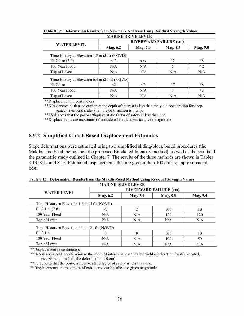
Table 8.12: Deformation Results from Newmark Analyses Using Residual Strength Values MARINE DRIVE LEVEE

RIVERWARD FAILURE (cm) WATER LEVEL

Mag. 6.2 Mag. 7.0 Mag. 8.5 Mag. 9.0

Time History at Elevation 1.5 m (5 ft) (NGVD) El. 2.1 m (7 ft) < 2 xxx 12 FS 100 Year Flood N/A N/A 5 < 2 Top of Levee N/A N/A N/A N/A

Time History at Elevation 6.4 m (21 ft) (NGVD) El. 2.1 m <2 <2 17 FS 100 Year Flood N/A N/A 7 <2 Top of Levee N/A N/A N/A N/A

**Displacement in centimeters **N/A denotes peak acceleration at the depth of interest is less than the yield acceleration for deep-

seated, riverward slides (i.e., the deformation is 0 cm). **FS denotes that the post-earthquake static factor of safety is less than one. **Displacements are maximum of considered earthquakes for given magnitude

8.9.2 Simplified Chart-Based Displacement Estimates

Slope deformations were estimated using two simplified sliding-block based procedures (the Makdisi and Seed method and the proposed Bracketed Intensity method), as well as the results of the parametric study outlined in Chapter 7. The results of the three methods are shown in Tables 8.13, 8.14 and 8.15. Estimated displacements that are greater than 100 cm are approximate at best.

Table 8.13: Deformation Results from the Makdisi-Seed Method Using Residual Strength Values MARINE DRIVE LEVEE

RIVERWARD FAILURE (cm) WATER LEVEL

Mag. 6.2 Mag. 7.0 Mag. 8.5 Mag. 9.0

Time History at Elevation 1.5 m (5 ft) (NGVD) El. 2.1 m (7 ft) <2 2 500 FS 100 Year Flood N/A N/A 120 120 Top of Levee N/A N/A N/A N/A

Time History at Elevation 6.4 m (21 ft) (NGVD) El. 2.1 m 0 0 300 FS 100 Year Flood N/A N/A 100 50 Top of Levee N/A N/A N/A N/A

**Displacement in centimeters **N/A denotes peak acceleration at the depth of interest is less than the yield acceleration for deep-seated,

riverward slides (i.e., the deformation is 0 cm). **FS denotes that the post-earthquake static factor of safety is less than one. **Displacements are maximum of considered earthquakes for given magnitude

176

Table 8.14: Deformation Results from the Bracketed Intensity Method Using Residual Strength Values MARINE DRIVE LEVEE

RIVERWARD FAILURE (cm) WATER LEVEL

Mag. 6.2 Mag. 7.0 Mag. 8.5 Mag. 9.0

Time History at Elevation 1.5 m (5 ft) (NGVD) El. 2.1 m (7 ft) 0 0 6 FS 100 Year Flood N/A N/A 2 0 Top of Levee N/A N/A N/A N/A

Time History at Elevation 6.4 m (21 ft) (NGVD) El. 2.1 m 0 0 4 FS 100 Year Flood N/A N/A <2 0 Top of Levee N/A N/A N/A N/A

**Displacement in centimeters **N/A denotes peak acceleration at the depth of interest is less than the yield acceleration for deep-seated,

riverward slides (i.e., the deformation is 0 cm). **FS denotes that the post-earthquake static factor of safety is less than one. **Displacements are maximum of considered earthquakes for given magnitude

Table 8.15: Deformation Results from the Parametric Study Outlined in Chapter 7. MARINE DRIVE LEVEE

RIVERWARD FAILURE (cm) WATER LEVEL

Mag. 6.2 Mag. 7.0 Mag. 8.5 Mag. 9.0

Time History at Elevation 1.5 m (5 ft) (NGVD) El. 2.1 m (7 ft) <2 10 10 120 100 Year Flood 0 3 50 60 Top of Levee 0 0 3 13

Time History at Elevation 6.4 m (21 ft) (NGVD) El. 2.1 m 0 <2 40 110 100 Year Flood 0 0 30 40 Top of Levee 0 0 <2 8

**Displacement in centimeters **N/A denotes peak acceleration at the depth of interest is less than the yield acceleration for deep-seated,

riverward slides (i.e., the deformation is 0 cm). **Displacements are maximum of considered earthquakes for given magnitude

8.9.3 Numerical Dynamic Analysis

The numerical modeling was accomplished utilizing the commercially available finite difference computer program FLAC (Itasca Consulting Group 1997) described in Chapter 6. The FLAC model is a non-linear, two-dimensional finite difference program capable of modeling both static and dynamic situations. The model was implemented in the same fashion as outlined in Chapter 6 and employed in the parametric studies described in Chapter 7.

177

The earthquake time histories used in the analyses were recorded during the Mw 6.2 Mammoth Lakes earthquake (Long Valley Dam station) and Mw 8.5 Michoacán earthquake (Aeropuerto station). The motions were scaled to 0.29g and 0.12g, respectively. The SHAKE91 program was used to generate time histories at elevation -18 m (the input location for the motions in FLAC). The damping of the earthquake motions for numerical stability utilized Rayleigh damping. The acceptable Rayleigh damping used in the models was determined from the validation studies to be 5% at 5 Hz. Any baseline drift in the earthquake motions has been removed from all of the presented FLAC displacements.

The ground motions computed with FLAC for the embankment and foundation soils (elevations 1.5m and 6.4m as previously referenced) differ from those computed using the SHAKE91 program for two primary reasons. First, the FLAC model employs a linear analysis for dynamic ground response while the SHAKE91 model is based on the equivalent linear approach. In addition, the FLAC program models the embankment in two dimensions as opposed to the 1D model used in SHAKE91. The end result of these important differences is that the ground motions computed with FLAC are greater than those computed with SHAKE91. FLAC motions at selected elevations in the model were as large as 50% to 90% greater than the values produced with SHAKE91. Effects such as 2D embankment response highlight the need to adjust results from 1D models with the results of case history data, 2D and 3D response analyses of similar earth structures, and sound engineering judgment.

The water within the soil was modeled directly and was allowed to flow during the static solutions. During the dynamic solutions excess pore pressures were allowed to generate, but the dissipation of these pore pressures during earthquake shaking was not modeled. Water outside the slope was modeled as boundary pore pressure; therefore hydrodynamic effects were not modeled.

The boundary conditions for the static solutions consisted of the bottom boundary being fixed in both the horizontal and vertical directions, while the sides of the model were treated as rollers (by fixing only the horizontal direction). During the dynamic analysis the bottom boundary was freed in the horizontal direction to allow application of the horizontal acceleration, and the sidewalls were treated as an infinite medium (free field), having the same properties as the adjacent model perimeter zones. Figure 8.22 shows the soil layering and the model grid used in the numerical model analyses. The soil properties used in the numerical model for the layers shown in the figure are given in Table 8.16.

Table 8.16: Soil Properties Used in the Numerical Model (see Figure 8.22 for layer number references).

LAYER NUMBER Soil Type Dry Mass Density

(kg/m3)

Angle of Internal Friction

(deg) Porosity Cohesion

(kPa) (N1)60

blows/30 cm

1 SP 1381 37 0.4 0 11 2 SM 1252 33 0.5 0 11 3 CL/SM 1211 30 0.55 0 5 4 SM-ML 1288 33 0.4 0 6 5 SM 1366 33 0.5 0 6 6 SP 1381 37 0.5 0 10 7 ML 1098 0 0.6 62 3 8 SP 1489 37 0.4 0 31

178

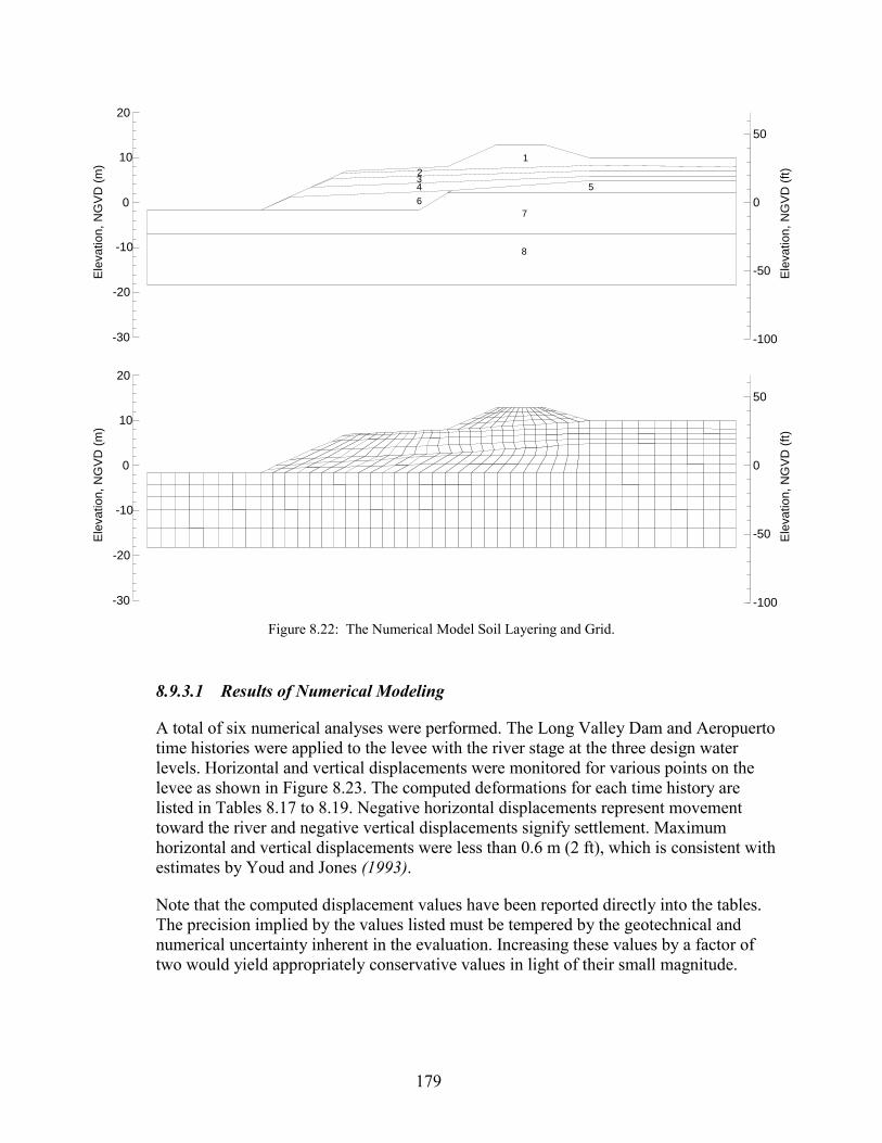
Elev

atio

n, N

GVD

(ft)

0

50

-50

-100

Elev

atio

n, N

GVD

(m)

0

10

20

-10

-20

-30

1234 5

76

8

Elev

atio

n, N

GVD

(ft)

0

50

-50

-100

Elev

atio

n, N

GVD

(m)

0

10

20

-10

-20

-30 Figure 8.22: The Numerical Model Soil Layering and Grid.

8.9.3.1 Results of Numerical Modeling

A total of six numerical analyses were performed. The Long Valley Dam and Aeropuerto time histories were applied to the levee with the river stage at the three design water levels. Horizontal and vertical displacements were monitored for various points on the levee as shown in Figure 8.23. The computed deformations for each time history are listed in Tables 8.17 to 8.19. Negative horizontal displacements represent movement toward the river and negative vertical displacements signify settlement. Maximum horizontal and vertical displacements were less than 0.6 m (2 ft), which is consistent with estimates by Youd and Jones (1993).

Note that the computed displacement values have been reported directly into the tables. The precision implied by the values listed must be tempered by the geotechnical and numerical uncertainty inherent in the evaluation. Increasing these values by a factor of two would yield appropriately conservative values in light of their small magnitude.

179

Top of Bench

Bottom of Bench

South Top of Embankment

North Bottomof Embankment South Bottom

of Embankment

North Topof Embankment

Approximate Levee Geometry

North (river) South (land)

Figure 8.23: Locations Where Displacements were Calculated in Numerical Model Analyses

Table 8.17: Deformation Results from Numerical Model Analyses with River Elev. at 2.1 m (7 ft) AEROPUERTO (0.12g) LONG VALLEY DAM (0.29g)

DISPLACEMENT LOCATION

Horizontal Displacement

(cm)

Vertical Displacement

(cm)

Horizontal Displacement

(cm)

Vertical Displacement

(cm) Bottom of bench -0.7 -3.4 -2.6 -4.8 Top of bench -1.5 -0.6 -8.1 -1.3 North bottom of embankment -0.6 -0.2 -6.4 -2.0 North top of embankment 0.1 -0.4 -5.5 -5.1 South top of embankment 0.2 -0.3 -0.3 -1.2 South bottom of embankment 0.3 -0.1 0.2 -0.3 Maximum for the embankment -1.0 -0.5 -7.2 -5.3 * Negative horizontal displacements represent movement toward the river and negative vertical

displacements signify settlement.

Table 8.18: Deformation Results from Numerical Model Analyses with River Elev. at 8.8 m (29 ft) AEROPUERTO (0.12g) LONG VALLEY DAM (0.29g)

DISPLACEMENT LOCATION

Horizontal Displacement

(cm)

Vertical Displacement

(cm)

Horizontal Displacement

(cm)

Vertical Displacement

(cm) Bottom of bench -2.3 -1.7 -5.1 -3.1 Top of bench -2.8 -0.4 -8.4 -0.8 North bottom of embankment -42.8 9.2 -48.9 10.1 North top of embankment -16.1 -11.0 -20.4 -13.5 South top of embankment -0.8 -1.9 -4.3 -6.3 South bottom of embankment 1.2 -0.1 0.9 0.4 Maximum for the embankment -42.8 -19.3 -48.9 -19.6 * Negative horizontal displacements represent movement toward the river and negative vertical

displacements signify settlement.

180

Table 8.19: Deformation Results from Numerical Model Analyses with River Elevation at the Crest AEROPUERTO (0.12g) LONG VALLEY DAM (0.29g)

DISPLACEMENT LOCATION

Horizontal Displacement

(cm)

Vertical Displacement

(cm)

Horizontal Displacement

(cm)

Vertical Displacement

(cm) Bottom of bench -0.7 -0.1 -2.0 -1.0 Top of bench -15.7 -1.0 -33.5 -2.0 North bottom of embankment -53.3 7.3 -55.6 3.1 North top of embankment -47.6 -49.3 -42.4 -54.4 South top of embankment 29.7 -11.9 38.5 -17.1 South bottom of embankment 38.3 11.7 50.2 18.0 Maximum for the embankment -82.4 -53.5 -79.3 -60.1 * Negative horizontal displacements represent movement toward the river and negative vertical

displacements signify settlement.

Two conclusions can be drawn from the results of the numerical modeling. First, the deformation of the levee gets progressively larger as the river elevation increases. As the river level increases, the phreatic surface also raises within the levee resulting in the saturation of more soil. These saturated soils are susceptible to excess pore pressure generation, resulting in larger levee deformations. Second, the deformations induced by the Long Valley Dam and Aeropuerto time histories are essentially the same for each river stage even though their respective PGA and duration values are significantly different. This indicates that the local shallow crustal earthquakes and subduction zone earthquakes are equally important for seismic hazard studies in this region.

8.9.4 Comparison of the Methods

Four methods have been utilized to estimate the earthquake-induced deformations of the Columbia River levee. In general, the simplified procedures for estimating lateral displacements provide a range of values that can be very useful for preliminary hazard evaluations. However, the displacements estimated using the Makdisi and Seed method, the Bracketed Intensity method, and the numerical modeling-based design chart (Figure 7.8) provided a broad range of values, particularly for cases involving large magnitude earthquakes and very low stability (i.e., low values of ky/kmax). The limitations of the Makdisi and Seed methods for these conditions have been discussed in several references (Makdisi and Seed 1978; Jibson 1993).

Table 8.20 presents a direct comparison between all of the methods using a Mw 8.5 earthquake motion for the three river stages analyzed. This includes the Newmark, Makdisi and Seed, and Bracketed Intensity analyses that used the time history at elevation 6.4 m. Note that for the three sliding block based methods, the deformations correspond to the movement of the entire slide mass (rigid body movement). The deformation for the method developed from the parametric study represents the maximum deformation. The numerical model displacement is the horizontal displacement of the north top of the levee (embankment).

181

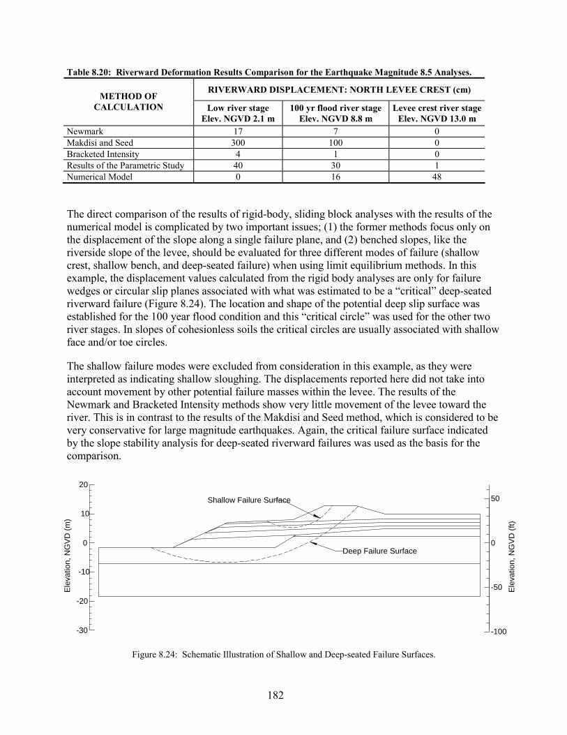
Table 8.20: Riverward Deformation Results Comparison for the Earthquake Magnitude 8.5 Analyses.

RIVERWARD DISPLACEMENT: NORTH LEVEE CREST (cm) METHOD OF

CALCULATION Low river stage Elev. NGVD 2.1 m

100 yr flood river stage Elev. NGVD 8.8 m

Levee crest river stageElev. NGVD 13.0 m

Newmark 17 7 0 Makdisi and Seed 300 100 0 Bracketed Intensity 4 1 0 Results of the Parametric Study 40 30 1 Numerical Model 0 16 48

The direct comparison of the results of rigid-body, sliding block analyses with the results of the numerical model is complicated by two important issues; (1) the former methods focus only on the displacement of the slope along a single failure plane, and (2) benched slopes, like the riverside slope of the levee, should be evaluated for three different modes of failure (shallow crest, shallow bench, and deep-seated failure) when using limit equilibrium methods. In this example, the displacement values calculated from the rigid body analyses are only for failure wedges or circular slip planes associated with what was estimated to be a “critical” deep-seated riverward failure (Figure 8.24). The location and shape of the potential deep slip surface was established for the 100 year flood condition and this “critical circle” was used for the other two river stages. In slopes of cohesionless soils the critical circles are usually associated with shallow face and/or toe circles.

The shallow failure modes were excluded from consideration in this example, as they were interpreted as indicating shallow sloughing. The displacements reported here did not take into account movement by other potential failure masses within the levee. The results of the Newmark and Bracketed Intensity methods show very little movement of the levee toward the river. This is in contrast to the results of the Makdisi and Seed method, which is considered to be very conservative for large magnitude earthquakes. Again, the critical failure surface indicated by the slope stability analysis for deep-seated riverward failures was used as the basis for the comparison.

Elev

atio

n, N

GVD

(ft)

0

50

-50

-100

Elev

atio

n, N

GVD

(m)

0

10

20

-10

-20

-30

Shallow Failure Surface

Deep Failure Surface

Figure 8.24: Schematic Illustration of Shallow and Deep-seated Failure Surfaces.

182

A relatively high factor of safety was determined for the deep slip circle, indicating a low probability for movement. However, the numerical model showed nearly 0.6 m of maximum movement by the levee toward the river, due to shallow modes of failure along the crest and bench of the levee. The movement computed by the model was largely associated with zones of deformation extending to a depth of approximately 1.5 m below the slope. These zones are more closely represented by shallow sloughing and shallow rotational modes of failure (not considered in the slope stability based analyses) indicated as critical in the limit equilibrium analyses. The deformations computed with the numerical model are, therefore, the sum of the displacements associated with all potential failure modes (i.e., shallow- and deep-seated deformations within the levee). It is not possible to isolate the displacements associated with each mode, as the deformation of the model grid reflects overall stability of the embankment. The Newmark, Makdisi and Seed, Bracketed Intensity, and parametric study results show that the deformations decrease with increasing river stage. This would be expected for stability analyses controlled by the undrained shear strengths of soils along the “critical” surface and rising external water levels that contribute stabilizing boundary pressures to the slope (this assumes that the undrained shear strength of the soil is unaffected by the rising water table). The numerical modeling results, however, indicate that deformations increase with increasing river stage, because the computed displacements account for the contributions of both shallow and deep-seated zones of deformation.

The displacement estimates from the rigid block analyses of rotational failure modes are also limited in that they are a summation of horizontal and vertical movement. Unfortunately, it is difficult to distinguish the relative contribution of each component to the overall displacement, making a direct comparison between these results and the numerical model estimates difficult. The numerical model provides a more representative pattern of slope and foundation deformations. These deformations vary from point to point; therefore, selecting a single displacement value to compare against the rigid-body methods is somewhat arbitrary. By selecting several locations on the levee, the deformations computed using the numerical model can be more readily compared to the results of the sliding block approaches. The data in Tables 8.20 and 8.21 provide a useful comparison of these methods and demonstrate the uncertainty associated with displacement estimates made using various widely-adopted procedures. The displacements computed using the numerical model indicate that the local M 6.2 crustal earthquake produces slope deformations that are equal to, or greater, than those induced by the distant M 8.5 earthquake. This again highlights the importance of accounting for both the intensity and duration of the strong ground motions. The relative slope deformations produced by these two scenario earthquakes will clearly vary depending on the source-to-site distances involved; therefore this general trend is not applicable to other regions of Oregon.

8.9.5 Application of Soil Improvement

The parametric study presented in Chapter 7 demonstrated that the effectiveness of soil improvement for minimizing lateral soil deformations during earthquakes can be reasonably estimated using standard limit equilibrium slope stability analysis and associated sliding block formulations provided that appropriate dynamic, or post-earthquake soil strengths are employed. More representative deformation estimates, however, can be obtained using the results of the combined limit equilibrium/numerical modeling studies (Figure 7.8). In these analyses, the zone of improved soil can be modeled as a either a homogeneous block of competent soil for broad

183

applications (DDC, closely spaced vibro-densification) or as discrete zones if ground techniques such as stone columns or grouting is employed. Representative soil strength parameters (�′, c′, su) must be estimated for the treated ground. It must be noted that this is a simplification of the field conditions for several reasons: (1) this method fails to account for the three dimensional aspect of ground treatment, (2) the stiffness of the treated soil is not incorporated into limit equilibrium analyses, and (3) excess pore pressures generated in the native soils will migrate into the improved soil, thereby decreasing effective stresses and soil strength.

On the basis of the analyses outlined in this example problem, it is clear that the potential exists for excessive soil deformations along the Columbia River levee. As mentioned, these seismically-induced displacements could impact bridge foundations, abutments, approach fills and roadways, limiting access following the design-level earthquakes. If the computed soil deformations exceed allowable limits, and bridge-specific criteria such as importance and cost-benefit for seismic strengthening (consistent with ODOT’s Liquefaction Mitigation Policy) indicate that remedial ground treatment is warranted, then the extent of the soil improvement must be determined. This will likely involve an iterative process of analysis wherein the width and location of the block of treated soils are modified until an optimal zone of improvement has been identified. The location and volume of treated soil will reflect the cost associated with the remedial ground improvement, the deformation limits for the embankment, and issues related to access and constructability (particularly around bridges and other overhead obstructions).

In practice, the effectiveness of ground treatment for reducing permanent deformations of the Columbia River levee in the region of interest can be evaluated by performing a series of analyses with varying widths of soil improvement. The cost of the ground treatment can then be related to the estimated seismic performance of the embankment. This allows for risk reduction strategies to be evaluated in terms of performance and serviceability, as well as cost effectiveness. For the sake of brevity, this sample problem adopted two ground treatment strategies for analysis. The zone of improvement extended across the full width of the upper portion of the levee and through the potentially liquefiable soil as illustrated in Figure 8.25. The improved soil was modeled as a uniform zone of dense sandy soil representing treatment by vibro-densification.

Again, this is a simplification of the actual three-dimensional pattern of densification that would result from closely spaced vibro-compaction. The improved soil was modeled as a dense ((N1)60 = 25 blows/30 cm), cohesionless material in which excess pore pressures would not be generated during cyclic loading. The soil dry mass density, angle of internal friction, and porosity were 1803 kg/m3, 37 deg, and 0.30, respectively for the zone of soil improvement. All other soils were modeled with the parameters used in the previous unimproved soil applications. Although it is clear that the ground treatment strategy employed in the design application would eliminate the liquefaction hazard directly beneath the levee, earthquake-induced deformations must still be evaluated in order to assess the seismic performance of the levee and associated transportation components.

184

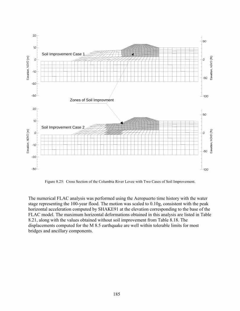
Soil Improvement Case 1

Soil Improvement Case 2

Zones of Soil Improvment

Figure 8.25: Cross Section of the Columbia River Levee with Two Cases of Soil Improvement.

The numerical FLAC analysis was performed using the Aeropuerto time history with the water stage representing the 100-year flood. The motion was scaled to 0.10g, consistent with the peak horizontal acceleration computed by SHAKE91 at the elevation corresponding to the base of the FLAC model. The maximum horizontal deformations obtained in this analysis are listed in Table 8.21, along with the values obtained without soil improvement from Table 8.18. The displacements computed for the M 8.5 earthquake are well within tolerable limits for most bridges and ancillary components.

185

Table 8.21: Comparison of Predicted Maximum Levee Displacements With and Without Soil Improvement at the 100 yr Flood Stage.

METHOD OF CALCULATION MAXIMUM HORIZONTAL

RIVERWARD LEVEE DISPLACEMENT (cm)

Without

Soil Improvement With Case 1

Soil Improvement With Case 2

Soil Improvement Newmark 7 0 0 Makdisi and Seed 100 N/A N/A Bracketed Intensity 1 0 0 Results of the Parametric Study 30 2 < 1 Numerical Model: N. Levee Crest 16 < 1 < 1 � Negative horizontal displacements represent movement toward the river and negative vertical displacements

signify settlement. � N/A denotes peak acceleration at the depth of interest is less than the yield acceleration for deep-seated,

riverward slides (i.e., the deformation is 0 cm).

8.10 SUMMARY AND CONCLUSIONS

The significant consequences associated with the failure of the Columbia River levee in the vicinity of the Interstate 5 and 205 bridges and Marine Drive provided the impetus for this thorough multi-hazard stability investigation. Standard of practice methods were used in conjunction with more sophisticated numerical models to assess the overall stability of the levee under static and dynamic loading conditions. The primary objectives of this investigation included: (1) evaluating the static stability of the levee at three different river stages; (2) assessing the seismic stability of the levee at the aforementioned water levels; (3) evaluating the potential extent of earthquake-induced deformations of the levee, and (4) indicating, in a general sense, the effectiveness of soil improvement for reducing seismically-induced deformations of the levee.

The following conclusions can be drawn based on this investigation.

Under static conditions, the levee appears to be stable at all sections with the river stage at the 100-year flood elevation or lower (elevation 8.8 m). However, landward failures due to high seepage forces were estimated to occur if the river was to reach the crest of the levee. The liquefaction hazard was considered to be minimal for a magnitude 6.2 earthquake however the generation of partial excess pore pressures combined with the higher intensity of ground motions produced permanent deformations that were similar to, or larger than those estimated for the larger scenario earthquakes. Conversely, the liquefaction hazard was greater for the distant, larger earthquakes but the destructiveness is limited somewhat by the low intensity of the motions. The silt rich soils in the levee and foundation are considered liquefiable based on cyclic laboratory tests performed on specimens from the site.

Under worst-case conditions, the levee is estimated to experience displacements of approximately 0.6 to 0.9 m (2-3 ft) based on the numerical modeling.

Simplified chart solutions for estimating seismically-induced deformations provided reasonable values from the standpoint of a preliminary screening for liquefaction hazards. It was

186

demonstrated that small deformation estimates based on simplified procedures are not necessarily an indication of acceptable seismic performance. In light of the resources necessary to conduct numerical analyses, it is recommended that several simplified methods of analysis be used to confirm the likely range of slope deformations due to design level ground motions.

A generalized numerical analysis of ground treatment demonstrated the effectiveness of soil improvement for reducing earthquake-induced embankment deformations to within tolerable limits.

8.11 LIMITATIONS AND RECOMMENDATIONS FOR FUTURE WORK

This example problem synthesized the results of existing geotechnical investigations and seismic hazard evaluations in order to perform an in-depth stability analyses of an embankment built of, and on, potentially liquefiable soils. Although a truly probabilistic, coupled, multi-hazard evaluation was beyond the scope of this example, the flood and earthquake scenarios have been selected to cover the broad range of conditions thought to affect the Columbia River levee adjacent to Hayden Island and interstate highway bridges. Standard-of-practice methods of analysis have been employed throughout this investigation. However, in light of the complexities associated with liquefaction hazards and slope stability, several simplifying assumptions have been made, as discussed in this chapter. It is anticipated that ODOT engineers will apply the methodology outlined here, as well as in seismic design guidelines, for projects throughout the state. For this reason, the following primary limitations of this investigation should be noted.

1. The results presented are based on the seismic hazard estimates recommended as of the date of this investigation. Changes to these estimates at a future date could alter the conclusions presented. Subsequent analyses may need to be performed using amended hazard scenarios.

2. Analyses were not performed on the deformed geometry of the levee. For the case of the river stage at the crest, soil deformations (slumping, sliding, settling) may reduce the seepage path through the levee, thereby creating high hydraulic gradients. Additional concerns such as sand boils and piping could occur. As a result, the levee might not be stable enough to allow the immediate regrading and/or other repairs that could be required to restabilize the levee. Additional seepage studies should be performed on the deformed geometry of the levee to evaluate these concerns.

3. Ground treatment by means of densification was the sole method evaluated in this example. Field applications have included stone columns for drainage and soft ground replacement, as well as grouting and soil-cement mixing techniques for stability and seepage cut-off. The seismic performance of these drainage and grouting/cement soil improvement methods have not been evaluated. It is recommended that these and other potentially effective liquefaction mitigation measures be evaluated, either independently or in combinations to assess the most cost effective ground treatment program.

187

9.0 SUMMARY AND CONCLUSIONS

Recent worldwide experience demonstrates the vulnerability of bridges to seismic and geologic hazards. Soil liquefaction causes the majority of damage to highway embankments and bridge components such as abutments, foundations and substructure. Earthquake-induced deformations of embankments and approach fills result in the loss of bridge operation which hinders post-earthquake response and recovery. Because of the importance of bridges as transportation lifelines and the impact of liquefaction on bridges, many transportation departments have adopted policies for liquefaction assessment and mitigation planning. The implementation of these policies requires a thorough understanding of liquefaction hazards and the potential damage modes to bridges and ancillary structures that are associated with liquefaction. Also, given the number of bridges in Oregon and the variety of structures involved, the need for a simplified, performance-based design method for implementing soil improvement at bridge sites has been demonstrated.

The primary objectives of this investigation were: (1) to provide a comprehensive review of post-earthquake reconnaissance reports in order to highlight potential liquefaction-induced damage modes at bridges; (2) to provide guidance on liquefaction hazard evaluations along with the most recent analysis methods used in practice; (3) to provide region-specific data on the liquefaction susceptibility of silty soils; (4) to outline a practice-oriented method for estimating lateral deformations of embankments with and without soil improvement; and (5) to provide an extensive, step-by-step design application for a site located in the Portland area. This hazard evaluation incorporated the most recent information on regional seismic hazards, cyclic behavior of sandy and silty soils, deformation estimates made by several approaches, and an evaluation of the effectiveness of soil improvement for improving the seismic performance of a riverfront embankment.

The “standard of practice” procedures for estimating seismically-induced ground deformations are based on pseudo-static, limit-equilibrium methods. Although these methods have been shown to provide reliable displacement estimates for competent soils, very few well-documented case studies involving liquefied soils have been presented. A study that incorporates conventional design approaches and numerical dynamic effective stress modeling has been conducted with the goal of developing a practice-oriented method for estimating seismically-induced deformations of slopes and embankments. The study involved determining the effects of varying several design parameters, including the embankment height, thickness of the liquefiable soil layer, extent of soil improvement, and ground motion characteristics. A simplified design chart was developed that allows engineers using standard analysis methods for static slope stability to estimate earthquake-induced deformations. The design chart provides a reasonable method for estimating lateral deformations of embankments with or without soil improvement. This design chart is applicable for the preliminary design of new embankments and for use as a screening tool for existing embankments.

189

9.1 RECOMMENDATIONS PERTINENT TO LIQUEFACTION HAZARD EVALUATIONS IN OREGON

1. From a practical perspective, the “failure” of highway embankments is directly related to magnitude of the permanent displacements experienced during an earthquake. The specification of “tolerable” deformations will reflect the sensitivity of the bridge abutments, foundation elements, and appurtenant structures.

2. Lateral soil deformations approaching 0.30 to 0.45 m (1 to 1.5 ft) should be viewed as problematic based on the review of field case studies in this investigation.

3. In light of the complexity of lateral spread phenomena, the uncertainty associated with free-field displacement estimates resulting from empirical and/or limit equilibrium, rigid body analyses is a factor of ±2. This approximate value is considered appropriate for sites that have been well characterized by in situ geotechnical testing procedures.

4. The factors of safety computed with limit-equilibrium methods are not adequately correlated with embankment deformations to facilitate reliable estimates of seismically-induced lateral displacements, without correlation to more rigorous numerical modeling methods (such as that presented in Figures 7.7 and 7.8).

5. In order to estimate embankment and foundation displacement the intensity and duration of the earthquake, and potential pore pressure generation in the embankment and foundation soils must be evaluated.

6. Seismic hazards in Oregon are rather unique in that they include contributions of interface subduction zone earthquakes, deep intra-plate subduction zone earthquakes, and shallow crustal earthquakes. Liquefaction hazards are a function of earthquake magnitude and ground motion duration. Therefore, liquefaction evaluations must incorporate the individual contributions of each of these seismic sources. Ground motion parameters from uniform hazard investigations must be amended to account for the relative contributions of the various seismic sources (the hazard must be de-aggregated).

7. A simplified method of estimating seismically-induced lateral deformations of embankments (applicable for both unimproved and improved soil sites) has been proposed. This method is intended to supplement and not supersede existing evaluation procedures. In light of the ease of use of the various procedures outlined in this report, it is recommended that two or more methods be applied as a means of assessing the range of likely embankment deformations.

8. In many cases, deformation limits for embankments will be small. Given the intensity and duration of ground motions indicated by recent seismic hazard investigations (particularly for western Oregon), it may not be possible to limit deformations to within tolerable limits utilizing only soil densification techniques. Ground treatment involving methods such as grouting, soil-cement mixing, replacement and drainage may be required. Foundation improvement with structural elements (e.g., piles, sheetpile cells) or

190

dewatering may be warranted. Additionally, structural retrofit and hardening also may be required.

9.2 GENERAL RECOMMENDATIONS FOR FUTURE WORK

1. The influence of pile groups on lateral ground deformation is poorly understood. In current practice, it is conservatively assumed that piles offer no lateral resistance to ground movement (free-field ground deformations are assumed). In light of the case studies reviewed, this is a prudent assumption for small pile groups. Field observations confirm that large pile groups can withstand lateral earth pressures due to movement of liquefiable soil and overlying “crusts” of competent soil. This issue is relevant for assessing the seismic performance of existing bridge foundations and the prioritization for remedial ground treatment given the number of bridges involved and the limited resources that are available for seismic rehabilitation.

2. The seismic performance of batter piles has been shown to be quite poor at sites exhibiting lateral ground deformation in excess of 0.15 to 0.3 m (0.5 to 1 ft). The performance of bridge abutments supported by batter piles should be reviewed.

3. The seismic performance of embankments with various soil improvement strategies (vibro-compaction, soil mixing, deep dynamic compaction) should be evaluated.

4. Recent investigations employing physical model testing (centrifuge, shake table) have been fruitful for augmenting the database of well documented case studies, the validation of numerical models, and for evaluating the effectiveness of soil improvement adjacent to bridge embankments and slopes. Continued work incorporating pile foundations is recommended.

5. The influence of long-duration motions, such as those associated with great Cascadia Subduction Zone earthquakes, on the performance of highway embankments and bridge components should be investigated.

191

10.0 REFERENCES

Abdoun, T., R. Dobry, T.D. O’Rourke, and D. Chaudhuri. (1996). “Centrifuge Modeling of Seismically-Induced Lateral Deformation During Liquefaction and its Effect on a Pile Foundation,” Proc. 6th Japan-U.S. Workshop on Earthquake Resistant Design of Lifeline Facilities and Countermeasures Against Soil Liquefaction, National Center for Earthquake Engineering Research, Technical Report NCEER-96-0012. pp. 525-540.

Abrahamson, N.A. and W.J. Silva. (1997). “Empirical Response Spectral Attenuation Relations for Shallow Crustal Earthquakes.” Seismological Research Letters 68(1):94-127.

Adalier, K., A.W. Elgamal, and G.R. Martin. (1998). “Foundation Liquefaction Countermeasures for Earth Embankments,” Journal of Geotechnical and Geoenvironmental Engineering 124(6):500-517.

Ambraseys, N.N. (1988). “Engineering Seismology,” Earthquake Engineering and Structural Dynamics 17(1):105.

Ambraseys, N.N. and J.M. Menu. (1988). “Earthquake-Induced Ground Displacements,” Earthquake Engineering and Structural Dynamics 16:985-1006.

Amini, F. and G.Z. Qi. (2000). “Liquefaction Testing of Stratified Silty Soils,” Journal of Geotechnical and Geoenvironmental Engineering 126(3):208-216.

Andrus, R.D. and K.H. Stokoe. (1997). “Liquefaction Resistance Based on Shear Wave Velocity,” Proceedings of the NCEER Workshop on Evaluation of Liquefaction Resistance of Soils”. National Center for Earthquake Engineering Research, Technical Report NCEER-97-0022. Salt Lake City, UT. pp. 89-128.

Arango, I. (1996). “Magnitude Scaling Factors for Soil Liquefaction Evaluations,” Journal of Geotechnical Engineering 122(11):929-936.

Ashford, S.A., K.M. Rollins, S.C. Bradford, T.J. Weaver, and J.I. Baez. (1999). “Liquefaction Mitigation Using Stone Columns Around Deep Foundations: Full Scale Test Results,” Dept. of Structural Engineering, Technical Report, Univ. of California, San Diego. 22 p.

Baez, J.I. (1995). “A Design Model for the Reduction of Soil Liquefaction by Vibro-Stone Columns,” Doctoral Dissertation in Civil Engineering, University of Southern California. 207 p.

Baez, J.I. and G.R. Martin. (1992). “Qualitative Evaluation of Stone Column Techniques for Earthquake Liquefaction Mitigation,” Proc. 10th World Conf. on Earthquake Engineering, A.A. Balkema Publ. pp. 1477-1483.

193

194

Bardet, J.P. (1990). “LINOS - A Non-Linear Finite Element Program for Geomechanics and Geotechnical Engineering,” Civil Engineering Dept., Univ. of Southern California.

Barksdale, R.D. (1987). “Applications of the State of the Art of Stone Columns –Liquefaction, Local Bearing Failure, and Example Calculations,” U.S. Army Corps of Engineers, Technical Report REMR-GT-7. 90 p.

Bartlett, S.F. and T.L. Youd. (1992). “Case Histories of Lateral Spreads Caused by the 1964 Alaska Earthquake,” Case Studies of Liquefaction and Lifeline Performance During Past Earthquake, Technical Report NCEER-92-0002, National Center for Earthquake Engineering Research, State University of New York, Buffalo. pp. 2.1-2.127.

Bartlett, S.F. and T.L. Youd. (1995). “Empirical Prediction of Liquefaction-Induced Lateral Spread,” Journal of Geotechnical Engineering 121(4):316-329.

Baziar, M.H., and R. Dobry. (1995). “Residual Strength and Large-Deformation Potential of Loose Silty Sands,” Journal of Geotechnical Engineering 121(12):896-906.

Baziar, M.H., R. Dobry, and M. Alemi. (1992). “Evaluation of Lateral Deformation using Sliding Block Model”, Proc. 10th World Conference on Earthquake Engineering, A.A. Balkema Publ. 3:1401-1406.

Baziar, M.H., R. Dobry, and A-W.M. Elgamel. (1992). “Engineering Evaluation of Permanent Ground Deformations Due to Seismically-Induced Liquefaction,” Technical Report NCEER-92-0007, National Center for Earthquake Engineering Research, State University of New York at Buffalo. 259 p.

Beaty, M. and P.M. Byrne. (1998). “An Effective Stress Model for Predicting Liquefaction Behavior of Sand,” Proc. of the Geotechnical Earthquake Engineering and Soil Dynamics III, ASCE Geotechnical Special Publication 75(1):766-777.

Blakely, R.J., R.E. Wells, T.S. Yelin, I.P. Madin, and M.H. Beeson, (1995). “Tectonic Setting of the Portland-Vancouver Area, Oregon and Washington: Constraints from Low-Altitude Aeromagnetic Data,” Geological Society of America Bulletin 107:1051-1062.

Boore, D.M., W.B. Joyner, and T.E. Fumal. (1997). “Equations for Estimating Horizontal Response Spectra and Peak Acceleration from Western North American Earthquakes: A Summary of Recent Work,” Seismological Research Letters 68(1):128-153.

Boulanger, R.W., C.J. Curras, B.L. Kutter, D.W. Wilson, and A. Abghari. (1999). “Seismic Soil-Pile-Structure Interaction Experiments and Analyses,” Journal of Geotechnical and Geoenvironmental Engineering 125(9):750–759.

Boulanger, R.W., and R.F. Hayden. (1995). “Aspects of Compaction Grouting of Liquefiable Soil,” Journal of Geotechnical Engineering 121(12):844-855.

195

Boulanger, R.W., I.M. Idriss, D.P. Stewart, Y. Hashash, and B. Schmidt. (1998). “Drainage Capacity of Stone Columns or Gravel Drains for Mitigating Liquefaction,” Proc. of the Geotechnical Earthquake Engineering and Soil Dynamics III, ASCE Geotechnical Special Publication 75(1):678-690.

Boulanger, R.W., M.W. Meyers, L.H. Mejia and I.M. Idriss. (1998). “Behavior of a Fine-grained Soil during the Loma Prieta Earthquake,” Canadian Geotechnical Journal 35:146-158.

Boulanger, R.W. and R.B. Seed. (1995). “Liquefaction of Sand Under Bidirectional Monotonic and Cyclic Loading.” Journal of Geotechnical Engineering 121(12):870-878.

Boulanger, R.W., D.P. Stewart, I.M. Idriss, Y. Hashash, and B. Schmidt. (1997). “Ground Improvement Issues for Posey & Webster St. Tubes Seismic Retrofit Project: Lessons from Case Histories,” Report No. UCD/CGM-97/03, Center for Geotechnical Modeling, Dept. of Civil & Environmental Engineering, Univ. of California, Davis. 125 p.

Brown, J. (in preparation). “Liquefaction Susceptibility and Post-Liquefaction Behavior of Silts,” Masters Thesis in Civil Engineering, Oregon State University, Corvallis.

Bruce, D.A. (2000). “An Introduction to the Deep Soil Mixing Methods as Used in Geotechnical Applications,” Federal Highway Administration, Publication No. FHWA-RD-99-138. 143 p.

Byrne, P.M., H. Jitno, D.L. Anderson, and J. Haile. (1994). “A Procedure for Predicting Seismic Displacements of Earth Dams,” Proc. of the 13th International Conference on Soil Mechanics and Foundation Engineering, New Delhi, India. pp. 1047-1052.

Byrne, P.M., H. Jitno, and F. Salgado. (1992). “Earthquake Induced Displacements of Soil-structures Systems,” Proc. 10th World Conf. on Earthquake Engineering, A.A. Balkema Publ. pp. 1407-1412.

Campanella, R.G. and W.P. Stewart. (1991). “Down-hole Seismic Cone Analysis Using Digital Signal Processing,” Proceedings, Second International Conference on Recent Advances in Geotechnical Earthquake Engineering and Soil Dynamics II, St. Louis, MO. pp. 77-82.

Campbell, K.W. 1997. “Empirical Near-Source Attenuation Relationships for Horizontal and Vertical Components of Peak Ground Acceleration, Peak Ground Velocity, and Pseudo Absolute Acceleration Response Spectra,” Seismological Research Letters 68(1):154-179.

Castro, G. (1975). “Liquefaction and Cyclic Mobility of Saturated Sands,” Journal of the Geotechnical Engineering Division 101(GT6):551-569.

Castro, G., T.O. Keller, and S.S. Boynton. (1989). “Re-Evaluation of the Lower San Fernando Dam - Report 1, An Investigation of the February 9, 1971 Slide,” Volume 1, Text; Volume 2, Appendixes A-F. U.S. Army Corps of Engineers, Contract Report GL-89-2. p. 439.

Castro, G. and S.J. Poulos. (1977). “Factors Affecting Liquefaction and Cyclic Mobility,” Journal of the Geotechnical Engineering Division 103(GT6):501-516.

196

California Division of Mines and Geology (CDMG). (1997). “Guidelines for Evaluating and Mitigating Seismic Hazards in California.” Special Publication 117, California Department of Conservation. 74 p.

Chang, N.Y. (1990). “Influence of Fine Content and Plasticity on Earthquake-Induced Soil Liquefaction,” Contract No. DACW3988-C-0078 to U.S. Army Engineer Waterways Experiment Station, Vicksburg, MS.

Cooke, H.G. and J.K. Mitchell. (1999). “Guide to Remedial Measures for Liquefaction Mitigation at Existing Highway Bridge Sites,” Multidisciplinary Center for Earthquake Engineering Research, Report No. MCEER-99-0015. 162 p.

Dickenson S.E., and J. Brown. (1997a). “Cyclic and Post-Cyclic Testing of Saturated, Alluvial Silts, Hayden Island, Oregon,” Final report on testing sponsored by GeoEngineers through Service and Testing Project, Dept. of Civil, Construction, and Environmental Engineering, Oregon State University, Corvallis.

Dickenson, S.E. and J. Brown. (1997b). “Cyclic and Post-Cyclic Testing of Saturated, Alluvial Silts, Port of Tacoma Road, Tacoma, WA,” Final report on testing sponsored by the Washington State Department of Transportation through Service and Testing Project, Dept. of Civil, Construction, and Environmental Engineering, Oregon State University.

Dickenson, S.E., B.J. Wavra, and J. Sunitsakul. (2000). “Seismic Performance of the Columbia River Levee Adjacent to the Portland International Airport (PDX), Portland, Oregon,” Report to the U.S. Army Corps of Engineers, Portland District. 113 p., plus appendices.

Dickenson, S.E. and D.S. Yang. (1998). “Seismically-Induced Deformations of Caisson Retaining Walls in Improved Soils,” Proceedings from the 1998 ASCE Geotechnical Earthquake Engineering and Soil Dynamics Conference. Seattle, WA. pp. 1071-1082.

Dobry, R. and M.H. Baziar. (1991). “Evaluation of Ground Deformation Caused By Lateral Spreading,” Proc. 3rd Japan-U.S. Workshop on Earthquake Resistant Design of Lifeline Facilities and Countermeasures for Soil Liquefaction, National Center for Earthquake Engineering Research, Technical Report NCEER-91-0001. pp. 209-223.

Dobry, R. and M.H. Baziar. (1992). “Modeling of Lateral Spreads in Silty Sands by Sliding Soil Blocks,” Proc. of Stability and Performance of Slopes and Embankments-II, ASCE Geotechnical Special Publication 31(1):625-652.

Dobry, R., R.S. Ladd, F.Y. Yokel, R.M. Chung, and D. Powell. (1982). “Prediction of Pore Water Pressure Buildup and Liquefaction of Sands During Earthquakes by the Cyclic Strain Method,” National Bureau of Standards Building Science Series 138. 150 p.

Dobry, R., K.H. Stokoe II, R.S. Ladd, and T.L. Youd. (1981). “Liquefaction Susceptibility From S-Wave Velocity,” Proceedings, Session on In-Situ Testing to Evaluate Liquefaction Susceptibility, ASCE National Convention, St Louis, MO.

197

Ebeling, R.M. and E.E. Morrison. (1993). “The Seismic Design of Waterfront Retaining Structures.” Naval Civil Engineering Laboratory, Technical Report ITL-92-11, Report No. NCEL TR-939. 255 p.

Edris, E.V. and S.G. Wright. (1994). “User’s Guide: UTEXAS3 Slope-Stability Package, Vol. 4: User’s Manual,” U.S. Army Corps of Engineers, Instruction Report GL-87-1. 268 p.

Egan, J.A., R.F. Hayden, L.L. Scheibel, M. Otus, and G. Serventi. (1992). “Seismic Repair at Seventh Street Marine Terminal,” Proc. of Grouting, Soil Improvement and Geosynthetics, pp. 867-878.

Evans, M.D. and L.F. Harder. (1993). “Liquefaction Potential of Gravelly Soils in Dams,” Geotechnical Practice in Dam Rehabilitation, ASCE Geotechnical Special Publication 35:467-481.

Evans, M.D. and S. Zhou. (1994). “Cyclic Behavior of Gravelly Soil,” Ground Failures Under Seismic Conditions, ASCE Geotechnical Special Publication 44:158-176.

Ferritto, J. (1997). “Seismic Design Criteria for Soil Liquefaction,” Technical Report TR-2077-SHR, U.S. Naval Facilities Engineering Services Center, Port Hueneme, CA. 58 p.

Ferritto, J.M. and J.B. Forrest. (1977). “Determination of Seismically-Induced Soil Liquefaction Potential at Proposed Bridge Sites; Vol II – Planning Guide for Evaluation of Liquefaction,” Federal Highway Administration, Report No. FHWA-RD-77-128. 134 p.

Federal Highway Administration (FHWA). (1985). “Tolerable Movement Criteria for Highway Bridges,” U. S. Department of Transportation, Report No. FHWA/RD-85-107. 109 p.

Finn, W.D.L. (1990). “Analysis of Deformations, Stability and Pore Water Pressures in Port Structures,” Proc. of the POLA Seismic Workshop on Seismic Engineering, Port of Los Angeles. pp. 369-391.

Finn, W.D.L., D.J. Pickering, D.J., and P.L. Bransby. (1971). “Sand Liquefaction in Triaxial and Simple Shear Tests.” Journal of the Soil Mechanics and Foundations Division 97(SM4):639-659.

Finn, W.D.L., K.W. Lee, and G.R. Martin. (1977). “An Effective Stress Model For Liquefaction,” Journal of the Geotechnical Engineering Division 103(6):517-533.

Finn, W.D.L., R.H. Ledbetter, and G. Wu. (1994). “Liquefaction of Silty Soils: Design and Analysis,” Ground Failures Under Seismic Conditions, ASCE Geotechnical Special Publication 44:51-76.

Francis, M.A. and G.A. Gorski. (1998). “In Situ Soil Mixing for the Mitigation of Seismic Lateral Spreading: A Case History,” Proc. of the Deep Foundation Institute Annual Meeting, Seattle, WA.

198

Fujii, S., M. Cubrinovski, K. Tokimatsu, and T. Hayashi. (1998). “Analyses of Damaged and Undamaged Pile Foundations in Liquefied Soils During the 1995 Kobe Earthquake,” Proc. of the Geotechnical Earthquake Engineering and Soil Dynamics III, ASCE Geotechnical Special Publication 75(2):1187-1198.

Geomatrix Consultants. (1995). “Seismic Design Mapping, State of Oregon.” Final Report, Prepared for the Oregon Department of Transportation. Project No.2442.

Gibbs, H.J. and W.G. Holtz. (1957). “Research on Determining the Density of Sands by Spoon Penetration Testing,” Proceedings, 4th International Conference on Soil Mechanics and Foundation Engineering, Vol. 1, London. pp. 35-39.

Guo, T. and S. Prakash. (1999). “Liquefaction of Silts and Silt-Clay Mixtures,” Journal of Geotechnical and Geoenvironmental Engineering 125(8):706-710.

Hamada, M. (1992). “Large Ground Deformations and Their Effects on Lifelines: 1964 Niigata Earthquake,” Case Studies of Liquefaction and Lifeline Performance During Past Earthquake, Technical Report NCEER-92-0001, National Center for Earthquake Engineering Research, State University of New York at Buffalo. pp. 3.1-4.123.

Hamada, M., S. Yasuda, R. Isoyama, and K. Emoto. (1986). “Study on Liquefaction Induced Permanent Ground Displacements,” Association for the Development of Earthquake Prediction, Research Committee Report, Tokyo, Japan. 87 p.

Hamada, M., R. Isoyama, K. Wakamatsu, (1995). “The 1995 Hyogoken-Nanbu (Kobe) earthquake: Liquefaction, Ground Displacement and Soil Condition in Hanshin Area,” Assoc. for Development of Earthquake Prediction, The School of Science and Engineering, Waseda University, and the Japan Engineering Consultants, Publ. by the Assoc. for Development of Earthquake Prediction. 194 p.

Hamada, M., R. Isoyama, and K. Wakamatsu. (1996). “Liquefaction-Induced Ground Damage and Its Related Damage to Lifeline Facilities,” Soils and Foundations – Special Issue on Geotechnical Aspects of the January 17 1995 Hyogoken-Nanbu Earthquake, Japanese Geotechnical Society. pp. 81-98.

Hannan, R. (2000). Personal communication, U.S. Army Corps of Engineers, Portland District.

Harder, L.F. (1988). “Use of Penetration Tests to Determine the Cyclic Load Resistance of Gravelly Soils,” Doctoral Dissertation in Civil Engineering, University of California, Berkeley.

Harder, L.F. (1994). “Becker test results From Gravel Liquefaction Sites,” Ground Failures Under Seismic Conditions, ASCE Geotechnical Special Publication 44:201-220.

Harder, L.F. and H.B. Seed. (1986). “Determination of Penetration Resistance For Coarse-Grained Soils Using the Becker Hammer-Drill,” Report No. UCB/EERC/86-06, Earthquake Engineering Research Center, University of California, Berkeley.

199

Horikoshi, K., H. Ohtsu, M. Tanaka, and T. Sueoka. (1997). “Centrifuge Modeling of a Pile Subjected to Lateral Spreading of Liquefied Soil,” Proc. of the 3rd Kansai International Geotechnical Forum on Comparative Geotechnical Engineering (KIG-Forum '97), Kobe, January, Publ. by the Kansai Branch of the Japanese Geotechnical Society. pp. 199-208.

Hryciw, R.D., editor. (1995). “Soil Improvement for Earthquake Hazard Mitigation,” ASCE Geotechnical Special Publication No. 49, New York, NY. 137 p.

Hyndman, R.D., and K. Wang. (1993). “Thermal Constraints on the Zone of Major Thrust Earthquake Failure: The Cascadia Subduction Zone,” Journal of Geophysical Research 98:2039-2060.

Hynes-Griffin, M.E., and A.G. Franklin. (1984). “Rationalizing the Seismic Coefficient Method,” U.S. Army Corps of Engineers Waterways Experiment Station. Miscellaneous Paper GL-84-13. Vicksburg, MS. 21 p.

Iai, S. (1998). “Seismic Analysis and Performance of Retaining Structures,” Proc. of the Geotechnical Earthquake Engineering and Soil Dynamics III, ASCE Geotechnical Special Publication 75(2):1020-1044.

Iai, S., Y. Matsunaga, T. Morita, H. Sakurai, H. Oishi, H. Ogura, Y. Ando, Y. Tanaka, and M. Kato. (1994). “Effects of Remedial Measures against Liquefaction at 1993 Kushiro-Oki Earthquake.” Proceedings of the Fifth US-Japan Workshop on Earthquake Resistant Design of Lifeline Facilities and Countermeasures Against Site Liquefaction. T.D. O’Rourke and M. Hamada (eds.). National Center for Earthquake Engineering Research. NCEER-94-0026. State University of New York, Buffalo. pp 135-152.

Idriss, I.M. and J.I. Sun. (1992). “User’s Manual for SHAKE91 – A Computer Program for Conducting Equivalent Linear Seismic Response Analyses of Horizontally Layered Soil Deposits,” Center for Geotechnical Modeling, Dept. of Civil & Environmental Engineering, Univ. of California, Davis.

Inel, S., W. Roth, and C. de Rubertis. (1993). “Nonlinear Dynamic Effective-Stress Analysis of Two Case Histories,” Proc. 3rd International Conf. on Case Histories in Geotechnical Engineering, St. Louis, MO. pp. 1735-1741.

Ishihara, K. (1985). “Stability of Natural Deposits During Earthquakes,” Proceedings, Eleventh International Conference on Soil Mechanics and Foundation Engineering, San Francisco, CA. A.A. Balkema Publ. pp. 321-376.

Ishihara, K. (1993). “Liquefaction and Flow Failure During Earthquakes,” Geotechnique, The Institution of Civil Engineers 43(3):351-415.

Ishihara, K. (1996). “Soil Behavior in Earthquake Geotechnics,” Clarendon Press, Oxford. 350 p.

Ishihara, K. and M. Cubrinovski. (1998a). “Problems Associated with Liquefaction and Lateral Spreading During Earthquakes,” Proc. of the Geotechnical Earthquake Engineering and Soil Dynamics III, ASCE Geotechnical Special Publication 75(1):301-312.

200

Ishihara, K. and M. Cubrinovski. (1998b). “Soil-pile Interaction in Liquefied Deposits Undergoing Lateral Spreading,” Geotechnical Hazards, Proc. of the 11th European Conf. on Soil Mechanics and Geotechnical Engineering, A.A. Balkema Publ. pp. 51-64.

Ishihara, K., and M. Yoshimine. (1992). “Evaluation of Settlements in Sand Deposits Following Liquefaction During Earthquakes,” Soils and Foundations, Japanese Society of Soil Mechanics and Foundation Engineering 32(1):173-188.

Itasca Consulting Group (1997). “User’s Manual for FLAC, v. 3.4,” Itasca. Minneapolis, MN.

Jackura, K. and A. Abghari. (1994). “Mitigation of Liquefaction Hazards at Three California Bridge Sites,” Proceedings of the Fifth US-Japan Workshop on Earthquake Resistant Design of Lifeline Facilities and Countermeasures Against Site Liquefaction. T.D. O’Rourke and M. Hamada (eds.). National Center for Earthquake Engineering Research. NCEER-94-0026. State University of New York, Buffalo. pp. 495-513.

Jafarzadeh, F. and E. Yanagisaw. (1998). “Behavior of the Saturated Sand Models in Two-directional Shaking Table Tests from Energy Point of View,” Proc. of the 11th European Conf. on Earthquake Engineering, A.A. Balkema. pp. 1-12.

Japanese Geotechnical Society. (1998). “Remedial Measures against Soil Liquefaction,” A.A. Balkema, Brookfield, 443 p.

Jibson, R.W. (1993). “Predicting Earthquake-Induced Landslide Displacements Using Newmark’s Sliding Block Analysis.” Transportation Research Record, No. 1411-Earthquake-Induced Ground Failure Hazards. Transportation Research Board. National Research Council. Washington, D.C. pp. 9-17.

Kachadoorian, R. (1968). “Effects of the Earthquake of March 27, 1964, on the Alaska Highway System,” U.S. Geological Survey Professional Paper 545-C, USGS; and The Great Alaska Earthquake of 1964 – Geology, Part A, “Effects on the Alaska Highway System,” National Academy of Sciences, Washington, D.C. pp. 641-703.

Kawasumi, H., editor. (1968). “General Report on the Niigata Earthquake of 1964,” publ. by the Tokyo Electrical Engineering College Press, Tokyo, Japan. 550 p., plus 148 plates.

Kayen, R.E. and J.K. Mitchell. (1998). “Assessment of Liquefaction Potential During Earthquakes by Arias Intensity,” Journal of Geotechnical and Geoenvironmental Engineering 123(12):1162-1174.

Kayen, R.E., W.A. Barnhardt, S.P. Palmer. (1998). “Geomorphological and Geotechnical Issues Affecting the Seismic Slope Stability of the Duwamish River Delta, Port of Seattle, Washington,” Proc. of the 5th U.S. Conference on Lifeline Earthquake Engineering – Optimizing Post-earthquake Lifeline System Reliability, ASCE-Technical Council on Lifeline Earthquake Engineering, Monograph No. 16. pp. 482-492.

201

Kayen, R.E., J.K. Mitchell, R.B. Seed, A. Lodge, S. Nishio, and R. Countinho. (1992). “Evaluation of SPT-, CPT-, and Shear Wave-Based Methods for Liquefaction Potential Assessment Using Loma Prieta Data,” Proceedings, Fourth Japan-U.S. Workshop on Earthquake Resistant Design of Lifeline Facilities and Countermeasures for Soil Liquefaction, Technical Report NCEER-92-0019, Honolulu, HI. pp. 177-204.

Keefer, D.K. and Y. Wang. (1997). “A Method for Predicting Slope Instability for Earthquake Hazard Maps: Preliminary Report.” Earthquakes – Converging at Cascadia, Symposium Proceedings. Associations of Engineering Geologists. Special Publication 10. pp. 39-52.

Koelling, M. and S.E. Dickenson. (1998). “Ground Improvement Case Histories for Liquefaction Mitigation at Port and Near-Shore Structures,” Proc. of the Geotechnical Earthquake Engineering and Soil Dynamics III, ASCE, Geotechnical Special Publication 75(1):614-626.

Koester, J.P. (1994). “Influence of Fines Type and Content on Cyclic Strength,” Ground Failures Under Seismic Conditions, ASCE Geotechnical Special Publication 44:17-33.

Kramer, S.L. (1996). “Geotechnical Earthquake Engineering,” Prentice Hall, NJ. 653 p.

Kramer, S.L. and M.W. Smith. (1997). “Modified Newmark Model for Seismic Displacements of Compliant Slopes,” Journal of Geotechnical and Geoenvironmental Engineering 123(7):635-644.

Ladd, R.S., R. Dobry, P. Dutko, F.Y. Yukol, and R.M. Chung. (1989). “Pore-Water Pressure Buildup in Clean Sands Because of Cyclic Straining,” ASTM Geotechnical Testing Journal 12(1):77-86.

Lam, P.I. and G.R. Martin. (1986a). “Seismic Design of Highway Bridge Foundations – Vol. I. Executive Summary,” Federal Highway Administration, Report No. FHWA/RD-86/101. 12 p.

Lam, P.I. and G.R. Martin. (1986b). “Seismic Design of Highway Bridge Foundations – Vol. II. Design Procedures and Guidelines,” Federal Highway Administration, Report No. FHWA/RD-86/102. 167 p.

Lam, P.I. and G.R. Martin. (1986c). “Seismic Design of Highway Bridge Foundations – Vol. III. Example Problems and Sensitivity Studies,” Federal Highway Administration, Report No. FHWA/RD-86/103. 145 p.

Law, K.T. and Y.H. Ling. (1992). “Liquefaction of Granular Soils with Non-cohesive and Cohesive Fines,” Proc. of the 10th World Conf. on Earthquake Engineering, A.A. Balkema Publ. 3:1491-1496.

Lawson, A.C., editor. (1908). “The California Earthquake of April 18, 1906: Report of the State Earthquake Investigation Commission,” Vol. 1, Part II, publ. by the Carnegie Institution of Washington. pp. 255-451.

Liao, S.C. and R.V. Whitman. (1985). “Overburden Correction Factors for SPT in Sand,” Journal of Geotechnical Engineering 112(3):373-377.

202

Liu, A.H. and J.P. Stewart. (1999). “Equivalent Number of Uniform Stress Cycles for Soil Liquefaction Analysis,” Pacific Earthquake Engineering Research Center 1999 Annual Meeting.

Lok, T.M. and M.F. Riemer. (1999). “Evaluation of Liquefaction Remediation Measures for Bridge Abutments.” Proc. of the International FLAC Symposium on Numerical Modeling in Geomechanics. C. Detournay and R. Hart eds. Minneapolis, MN, pp 357-363.

Lum, K.K.Y. and L. Yan. (1994). “In-situ Measurements of Dynamic Soil Properties and Liquefaction Resistances of Gravelly Soils at Keenleyside Dam,” Ground Failures Under Seismic Conditions, ASCE Geotechnical Special Publication 44:221-240.

Lysmer, J. et al. (1975). “FLUSH – A Computer Program for Approximate 3-D Analysis of Soil-Structure Interaction Problems,” EERC-UCB Report 75-30, Earthquake Engineering Research Center, Univ. of California, Berkeley.

Mabey, M.A. and I.P. Madin. (1992). “Shear Wave Velocity Measurements in the Willamette Valley and the Portland Basin, Oregon,” Oregon Geology 54(3):51-53.

Mabey, M.A. and I.P. Madin. (1995). “Downhole and Seismic Cone Penetrometer Shear-wave Velocity Measurements for the Portland Metropolitan Area, 1993 and 1994,” Oregon Department of Geology and Mineral Industries Open-File Report O-95-7.

Makdisi, F.I., and H.B. Seed. (1978). “Simplified Procedure for Estimating Dam and Embankment Earthquake-induced Deformations.” Journal of the Geotechnical Engineering Division, 104(7):849-867.

Manyando, G.M.S., T.L. Cooling, W.L. Durbin, and R.E. Anderson. (1993). “Liquefaction Mitigation Design, I-57 Mississippi River Bridge, Cairo, Illinois,” Proc. National Earthquake Conference, - Earthquake Hazard Reduction in the Central and Eastern United States: A Time for Examination and Action, Memphis, TN. pp. 659-668.

Marcuson, W.F., M.E. Hynes, and A.G. Franklin. (1990). “Evaluation of the Use of Residual Strength in Seismic Safety Analysis of Embankments,” Earthquake Spectra, 6(3):529-572.

Marcuson, W.F., M.E. Hynes, and A.G. Franklin. (1992). “Seismic Stability and Permanent Deformation Analyses: the Last Twenty Five Years,” Proc. of Stability and Performance of Slopes and Embankments-II, ASCE Geotechnical Special Publication 31(1):552-592.

Martin, G.R., W.D.L. Finn, and H.B. Seed. (1975). “Fundamentals of Liquefaction Under Cyclic Loading,” Journal of the Geotechnical Engineering Division, 101(GT5):423-483.

Martin, P.P. and H.B. Seed. (1979). “Simplified Procedure For Effective Stress Analysis of Ground Response,” Journal of the Geotechnical Engineering Division, 105(GT6):739-758.

Matsui, T. and K. Oda. (1996). “Foundation Damage to Structures,” Soils and Foundations – Special Issue on Geotechnical Aspects of the January 17 1995 Hyogoken-Nambu Earthquake, Japanese Geotechnical Society. pp. 189-200.

203

McCulloch, D.S. and M.G. Bonilla. (1970). “Effects of the Earthquake of March 27, 1964, on the Alaska Railroad,” U.S. Geological Survey Professional Paper 545-D, USGS, 161 p.; and The Great Alaska Earthquake of 1964 – Geology, Part A, “Effects on the Alaska Railroad,” National Academy of Sciences, Washington, D.C. pp. 543- 640.

McCullough, N.J. and S.E. Dickenson. 1998. “Estimation of Seismically-Induced Lateral Deformations for Anchored Sheetpile Bulkheads.” Proceedings from the 1998 ASCE Geotechnical Earthquake Engineering and Soil Dynamics Conference, Seattle, WA. pp. 1095-1106.

Meyerson, W.D., T.D. O'Rourke, and F. Miura. (1992). “Lateral Spread Effects on Reinforced Concrete Piles,” Proceedings, Fifth U.S.-Japan Workshop on Earthquake Disaster Prevention for Lifeline Systems, Tsukuba, Japan.

Mitchell, J.K., H.G. Cooke, and J.A. Schaeffer. (1998). “Design Considerations in Ground Improvement for Seismic Risk Mitigation,” Proc. of the Geotechnical Earthquake Engineering and Soil Dynamics III, ASCE Geotechnical Special Publication 75(1):580-613.

Miura, F. and T.D. O'Rourke. (1991). “Nonlinear Analyses of Piles Subjected to Liquefaction-Induced Large Ground Deformation,” Proceedings, Third Japan-U.S. Workshop on Earthquake-Resistant Design of Lifeline Facilities and Countermeasures for Soil Liquefaction, Technical Report NCEER-91-0001, State University of New York at Buffalo. pp 497-512.

Moriwaki, Y., P. Tan, and J. Feng. (1998). “Seismic Deformation Analysis of the Upper San Fernando Dam Under the 1971 San Fernando Earthquake,” Proc. of the Geotechnical Earthquake Engineering and Soil Dynamics III, ASCE Geotechnical Special Publication 75(2):854-865.

Muraleetharan, K.K., C. Mish, K. Yogachandran, and Arulanandan (1988). “DYSAC2: Dynamic Soil Analysis Code for 2-dimensional Problems,” Dept. of Civil Engineering, Univ. of California, Davis.

Naesgaard, E., P.M. Bryne, G. Ven Huizen. (1998). “Behavior of Light Structures Founded on Soil ‘Crust’ Over Liquefied Ground,” Proc. of the Geotechnical Earthquake Engineering and Soil Dynamics III, ASCE Geotechnical Special Publication 75(1):422-433.

National Research Council (NRC). (1985). “Liquefaction of Soils During Earthquakes,” National Research Council, National Science Foundation, Washington, D.C. 240 p.

Newmark, N. (1965). “Effects of Earthquakes on Dams and Embankments.” Geotechnique 15(2):139-160.

Oregon Board of Geologist Examiners/Oregon Board of Examiners for Engineering and Land Surveying (OBGE/OBEELS). (1997). “Guidelines for Site-specific Seismic Hazard Reports for Essential and Hazardous Facilities and Major and Special-occupancy Structures in Oregon,” Oregon Boards of Geologist Examiners and Examiners for Engineering and Land Surveying, Oregon Geology 59(1):6-8.

204

Oregon Department of Transportation (ODOT). (1996). “Liquefaction Mitigation Policy”, Oregon Department of Transportation, Bridge Engineering Section, Foundation Design Unit. 6 p.

Olsen, R.S. 1997. “Cyclic Liquefaction Based on the Cone Penetrometer Test.” Proceeding of the NCEER Workshop on Evaluation of Liquefaction Resistance of Soils. Technical Report NCEER-97-0022, Salt Lake City, UT. pp.225-276.

O’Rourke, T.D., W.D. Meyersohn, Y. Shiba, and D. Chaudhuri. (1994). “Evaluation of Pile Response to Liquefaction-Induced Lateral Spread,” Proceedings from the Fifth U.S.-Japan Workshop on Earthquake Resistant Design of Lifeline Facilities and Countermeasures Against Soil Liquefaction, Technical Report NCEER-97-0026, National Center for Earthquake Engineering Research, State University of New York at Buffalo. pp. 457-479.

O'Rourke, T.D. and J.W. Pease. (1992). “Large Ground Deformations and Their Effects on Lifeline Facilities: 1989 Loma Prieta Earthquake,” Case Studies of Liquefaction and Lifeline Performance During Past Earthquake, Technical Report NCEER-92-0002, National Center for Earthquake Engineering Research, State University of New York at Buffalo. pp. 5.1-5.85.

Plewes, M.D., E.C. McRoberts, and W.K. Chan. (1988). “Downhole Nuclear Density Logging in Sand Tailings,” Proceedings, ASCE Specialty Conference on Hydraulic Fill, Fort Collins, CO. pp. 290-309.

Port and Harbour Research Institute (PHRI). (1997). “Handbook on Liquefaction Remediation of Reclaimed Land,” A.A. Balkema Publ., Brookfield, VT, 312 p.

Poulos, S. (1981). “The Steady State of Deformation,” Journal of the Geotechnical Engineering Division 107(GT5):553-561.

Poulos, S.J., G. Castro, and J.W. France. (1985). “Liquefaction Evaluation Procedure,” Journal of Geotechnical Engineering 111(6):772-791.

Prakash, S., T. Guo, and S. Kumar. (1998). “Liquefaction of Silts and Silt-Clay Mixtures,” Proc. of the Geotechnical Earthquake Engineering and Soil Dynamics III, ASCE Geotechnical Special Publication 75(1):337-348.

Prakash, S. and P. Dakoulas, editors. (1994). “Ground Failures Under Seismic Conditions,” ASCE Geotechnical Special Publication No. 44. 261 p.

Rauch, A.F. and J.M. Martin. (2000). “EPOLLS Model for Predicting Average Displacements on Lateral Spreads,” Journal of Geotechnical and Geoenvironmental Engineering 126(4):360-371.

Reese, L.C. and S. Wang. (1994). “Documentation of Computer Program LPILE,” Ensoft, Inc. Vers 4.0. Austin, TX, 366 p.

Riemer, M.F., T.M. Lok, and J.K. Mitchell. (1996). “Evaluating Effectiveness of Liquefaction Remediation Measures for Bridges,” Proc. 6th Japan-U.S. Workshop on Earthquake Resistant Design of Lifeline Facilities and Countermeasures Against Soil Liquefaction, National Center for Earthquake Engineering Research, Technical Report NCEER-96-0012. pp. 441-455.

205

Robertson, P.K. and R.G. Campanella. (1985). “Liquefaction Potential of Sands Using the CPT,” Journal of Geotechnical Engineering 111(3):384-403.

Robertson, P.K., R.G. Campanella, D. Gillespie, and A. Rice. (1986). “A Seismic CPT to Measure In-Situ Shear Wave Velocity,” ASCE, Journal of the Geotechnical Engineering Division 112(8):791-803.

Robertson, P.K., D.J. Woeller, and W.D.L. Finn. (1992). “Seismic Cone Penetration Test for Evaluating Liquefaction Potential Under Cyclic Loading,” Canadian Geotechnical Journal 29:686-695.

Robertson, P.K. and C.E. Wride. (1997a). “Cyclic Liquefaction and Its Evaluation Based on the SPT and CPT,” Proceeding of the NCEER Workshop on Evaluation of Liquefaction Resistance of Soils. Technical Report NCEER-97-0022. Salt Lake City, UT. pp. 41-87.

Robertson, P.K. and C.E. Wride. (1997b). “Evaluation of Cyclic Liquefaction Potential Based on the CPT” Seismic Behavior of Ground and Geotechnical Structures, Seco e Pinto (ed.), A.A. Balkema, Brookfield, pp. 269-277

Ross, G.A., H.B. Seed, and R.R. Migliaccio. (1973). “Performance of Highway Bridge Foundations,” The Great Alaska Earthquake of 1964: Engineering, National Academy of Sciences, Washington, D.C. pp. 191-242.

Roth, W., H. Fong, and C. de Rubertis. (1992). “Batter Piles and the Seismic Performance of Pile-Supported Wharves,” Proc. of Ports ’92, 1:336-349, Seattle, WA.

Roth, W.H. and S. Inel. (1993). “An Engineering Approach to the Analysis of VELACS Centrifuge Tests,” Verifications of Numerical Procedures for the Analysis of Soil Liquefaction Problems. Arulanandan and Scott (eds.). A.A. Balkema, Rotterdam. pp. 1209-1229.

Roth, W., S. Inel, C. Davis, and G. Brodt. (1993). “Upper San Fernando Dam 1971 Revisited,” Proc. 10th Annual Conf. of the Assoc. of State Dam Safety Officials, Kansas City, MO. 12 p.

Roth, W., R.F. Scott, and P.A. Cundall. (1986). “Nonlinear Dynamic Analysis of a Centrifuge Model Embankment,” Proc. of the 3rd U.S. National Conf. on Earthquake Engineering, Charleston, SC. 12 p.

Sarma, S.K. (1975). “Seismic Stability of earth Dams and Embankments,” Geotechnique 25(4):743-761.

Sarma, S.K. and M.V. Bhave. (1974). “Critical Acceleration Versus Static Factor of Safety in Stability Analysis of Earth Dams and Embankments,” Geotechnique 24:661-665.

Sasaki, Y., W.D.L. Finn, A. Shibano, M. Nobuoto. (1996). “Settlement of Embankment Above a Liquefied Ground Which is Covered by Non-Liquefiable Surface Layer,” Proc. 6th Japan-U.S. Workshop on Earthquake Resistant Design of Lifeline Facilities and Countermeasures Against Soil Liquefaction, National Center for Earthquake Engineering Research, Technical Report NCEER-96-0012. pp. 361-390.

206

Schnabel, P., J. Lysmer, and H.B. Seed. (1972). “SHAKE – A Computer Program for Earthquake Response Analysis of Horizontally Layered Sites,” Earthquake Engineering Research Center, Report No. EERC 72-12, Univ. of California. 88 p.

Seed, H.B. (1979). “Considerations in the Earthquake-resistant Design of Earth and Rockfill Dams,” Geotechnique 29(3):215-263.

Seed, H.B. (1979). “Soil Liquefaction and Cyclic Mobility Evaluation for Level Ground During Earthquakes,” Journal of the Geotechnical Engineering Division 105(GT2):201-255.

Seed, H.B. (1987). “Design Problems in Soil Liquefaction,” Journal of the Geotechnical Engineering Division 113(8):827-845.

Seed, R.B. (1992). “A Manual for Evaluation and Mitigation of Liquefaction During Earthquakes,” Dept. of Civil Engineering, Univ. of California, Berkeley. 79 p.

Seed, H.B. and P. DeAlba. (1986). “Use of SPT and CPT Tests for Evaluating the Liquefaction Resistance of Sands,” ASCE Geotechnical Special Publication No. 6, Use of In Situ Tests In Geotechnical Engineering, New York, NY. pp. 281-301.

Seed, R.B. and L.F. Harder Jr. (1990). “SPT-Based Analysis of Cyclic Pore Pressure Generation and Undrained Residual Strength,” Proceedings, H. Bolton Seed Memorial Symposium, Vol. 2, BiTech Publishing, Vancouver, B.C. pp. 351-376.

Seed, H.B. and I.M. Idriss. (1971). “A Simplified Procedure for Evaluating Soil Liquefaction Potential,” Journal of the Soil Mechanics and Foundation Engineering Division 97(SM9):1249-1274.

Seed, H.B. and I.M. Idriss. (1982). “Ground Motions and Soil Liquefaction During Earthquakes,” EERI Monograph, Earthquake Engineering Research Institute. 134 p.

Seed. R.B. and H.L. Jong. (1987). “Factors Affecting Post-liquefaction Strength Assessment,” Proceedings, Fifth Canadian Conference on Earthquake Engineering, Ottawa, Canada. pp. 483-492.

Seed, H.B. and W.H. Peacock. 1971. “Test Procedures for Measuring Soil Liquefaction Characteristics.” Journal of the Soil Mechanics and Foundations Division 97(SM8):1099-1119.

Seed, H.B., I.M. Idriss, F. Makdisi, and N. Banerjee. (1975). “Representation of Irregular Stress Time Histories by Equivalent Uniform Stress Series in Liquefaction Analyses.” EERC 75-29. Earthquake Engineering Research Center, University of California, Berkley.

Seed, H.B., P.P. Martin, and J. Lysmer. (1976). “Pore-Pressure Changes During Soil Liquefaction.” Journal of the Geotechnical Engineering Division 102(GT4):323-345.

Seed, H.B., R.T. Wong, I.M. Idriss, and K. Tokimatsu. (1984). “Moduli and Damping Factors for Dynamic Analyses of Cohesionless Soils.” Earthquake Engineering Research Center, Report No. UCB/EERC-84/14, University of California, Berkeley. 37 p.

207

Seed, H.B., K. Tokimatsu, L.F. Harder, and R.M. Chung. (1985). “Influence of SPT Procedures in Soil Liquefaction Resistance Evaluations,” Journal of Geotechnical Engineering 111(12):1425-1445.

Seed, R.B., S.E. Dickenson, M.F. Riemer, J.D. Bray, N. Sitar, J.K. Mitchell, I.M. Idriss, R.E. Kayan, A. Kropp, L.F. Harder, Jr., and M.S. Power. (1990). “Preliminary Report on the Principal Geotechnical Aspects of the October 17, 1989 Loma Prieta Earthquake,” Report No. UCB/EERC-90/05, Earthquake Engineering Research Center, University of California at Berkeley. 139 p.

Seed, R.B., S.E. Dickenson, and C.M. Mok. (1994). “Site Effects on Strong Shaking and Seismic Risk: Recent Developments and Their Impact on Seismic Design Codes and Practice,” Proc. of Structures Congress XII. 1:573-579.

Shea, G.H., editor. (1991). “Costa Rica Earthquake Reconnaissance Report,” Earthquake Spectra, Supplement B, Vol. 7, Chapter 6 – Bridges, October, EERI, Oakland, CA. 127 p.

Shibata, T., F. Oka, and Y. Ozawa. (1996). “Characteristics of Ground Deformation due to Liquefaction,” Soils and Foundations – Special Issue on Geotechnical Aspects of the January 17 1995 Hyogoken-Nambu Earthquake, Japanese Geotechnical Society. pp. 65-80.

Shinozuka, M., editor. (1995). “The Hanshin-Awaji Earthquake of January 17, 1995 Performance of Lifelines,” Technical Report NCEER-95-0015, National Center for Earthquake Engineering Research, State University of New York at Buffalo. 286 p.

Silver, M.L. and H.B. Seed. (1971). “Volume Changes in Sands During Cyclic Loading,” Journal of the Soil Mechanics and Foundation Division 97(SM9):1171-1182.

Singh, S. (1994). “Liquefaction Characteristics of Silts,” Ground Failures Under Seismic Conditions, ASCE Geotechnical Special Publication 44:105-116.

Stark, T.D. and G. Mesri. (1992). “Undrained Shear Strength of Liquefied Sands For Stability Analysis,” Journal of Geotechnical Engineering 118(11):1727-1747.

Stark, T.D., S.M. Olson, S.L. Kramer, and T.L. Youd, editors. (1997). “Final Proceedings of the Workshop – Shear Strength of Liquefied Soils,” National Science Foundation Workshop, NSF Grant CMS-95-31678, 80 p., available from the Mid-America Earthquake Center at http://mae.ce.uiuc.edu/.

Stewart, D.P., R.W. Boulanger, I.M. Idriss, Y. Hashash, and B. Schmidt. (1997). “Ground Improvement Issues for Posey & Webster St. Tubes Seismic Retrofit Project: Lessons from Physical Modeling Studies,” Report No. UCD/CGM-97/04, Center for Geotechnical Modeling, Dept. of Civil & Environmental Engineering, Univ. of California, Davis. 117 p.

Stokoe II, K.H., J.M. Roesset, J.G. Bierschwale, and M. Aouad. (1989). “Liquefaction Potential of Sands From Shear Wave Velocity,” Proceedings, Ninth World Conference on Earthquake Engineering, Vol. III, Tokyo, Japan. pp. 213-218.

208

Sun, I.H. and I.M. Idriss. (1992). “User’s Manual for SHAKE91,” Center for Geotechnical Modeling, Department of Civil and Environmental Engineering, University of California, Davis.

Tokimatsu, K. and H.B. Seed. (1987). “Evaluation of Settlements in Sands Due to Earthquake Shaking,” Journal of Geotechnical Engineering 113(8):861-878.

Tokimatsu, K. and A. Uchida. (1990). “Correlation Between Liquefaction Resistance and Shear Wave Velocity,” Soils and Foundations 30(2):33-42.

Tokimatsu, K., H. Mizuno, and M. Kakurai. (1996). “Building Damage Associated with Geotechnical Problems,” Soils and Foundations – Special Issue on Geotechnical Aspects of the January 17 1995 Hyogoken-Nambu Earthquake, Japanese Geotechnical Society. pp. 219-234.

Tokimatsu, K., H. Oh-Oka, Y. Shamoto, A. Nakazawa, and Y. Asaka. (1997). “Failure and Deformation Modes of Piles Caused by Liquefaction-Induced Lateral Spreading in 1995 Hyogoken-Nambu Earthquake,” Proc. of the 3rd Kansai International Geotechnical Forum on Comparative Geotechnical Engineering (KIG-Forum '97), Kobe, January, Publ. by the Kansai Branch of the Japanese Geotechnical Society. pp. 239-248.

Tokimatsu, K., H. Oh-Oka, K. Satake, Y. Shamoto, and Y. Asaka, Y. (1998). “Effects of Lateral Ground Movements on Failure Patterns of Piles in the 1995 Hyogoken-Nambu Earthquake,” Proc. of the Geotechnical Earthquake Engineering and Soil Dynamics III, ASCE Geotechnical Special Publication 75(2):1175-1186.

U.S. Army Corps of Engineers. (1957).

United States Geologic Survey (USGS). (2000). National Hazard Mapping Project, United States Geologic Survey, http://geohazards.cr.usgs.gov/eq/.

Vessely, D.A., M. Riemer, I. Arango. (1996). “Liquefaction Susceptibility of Soft Alluvial Silts in the Willamette Valley,” Oregon Geology 58(6):14 p.

Vucetic, M. and R. Dobry. 1991. “Effect of Soil Plasticity on Cyclic Response,” Journal of Geotechnical Engineering 117(1):89-107.

Wang, S.T. and L.C. Reese. (1998). “Design of Pile Foundations in Liquefied Soils,” Proc. of the Geotechnical Earthquake Engineering and Soil Dynamics III, ASCE Geotechnical Special Publication 75(2):1331-1343.

Wilson, R.C. and D.K. Keefer. (1985). “Predicting Area Limits of Earthquake-Induced Landsliding,” Evaluating Earthquake Hazards in the Los Angeles Region. J.I. Ziony (ed.). USGS Professional Paper 1360. Reston, VA. pp. 317-345.

Wong, I.G. and W.J. Silva. (1993). “Strong Ground Shaking in the Portland, Oregon, Metropolitan Area: Evaluating the Effects of Local Crustal and Cascadia Subduction Zone Earthquakes and Near-Surface Geology,” Oregon Geology 55(6):137-143.

209

Wong, I.G., W.J. Silva, J. Bott, D. Wright, P. Thomas, N. Gregor, S. Li, M Mabey, A. Sojourner, and Y. Wang. (2000). “Earthquake Scenario and Probabilistic Ground Shaking Maps for the Portland, Oregon, Metropolitan Area.” IMS-16, Interpretive Map Series, Oregon Department of Geology and Mineral Industries, Portland, OR.

Yang, D.S. (1999). “Deformation-Based Seismic Design Models for Waterfront Structures,” Doctoral Dissertation in Civil, Construction and Environmental Engineering, Oregon State University, Corvallis. 260 p.

Yasuda, F., A. Nanjoh, and K. Kosa. (1997). “Investigation and Checking of Load Bearing Capacity of Damaged Piles,” Proc. of the 3rd Kansai International Geotechnical Forum on Comparative Geotechnical Engineering (KIG-Forum '97), Kobe, January, Publ. by the Kansai Branch of the Japanese Geotechnical Society. pp. 249-257.

Yasuda, S., K. Ishihara, K. Harada, N. Shinkawa. (1996). “Effect of Soil Improvement on Ground Subsidence Due to Liquefaction,” Soils and Foundations – Special Issue on Geotechnical Aspects of the January 17, 1995 Hyogoken-Nambu Earthquake, Japanese Geotechnical Society. pp. 99-107.

Yegian, M.K., E.A. Marciano and V.G. Ghahraman. (1991). “Earthquake-Induced Permanent Deformations: Probabilistic Approach,” Journal of Geotechnical Engineering 117(1):35-50.

Youd, T.L. (1972). “Compaction of Sands by Repeated Shear Straining,” Journal of the Soil Mechanics and Foundation Division 98(SM7):709-725.

Youd, T.L. (1991). “Mapping of Earthquake-Induced Liquefaction For Seismic Zonation,” Proceedings of the Fourth International Conference on Seismic Zonation, Earthquake Engineering Research Institute, Stanford, CA. pp. 112-147.

Youd, T.L. (1993). “Liquefaction-Induced Damage to Bridges,” Transportation Research Record 1411, Transportation Research Board, National Research Council, Washington, D.C. pp. 35-41.

Youd, T.L. (1998). “Screening Guide for Rapid Assessment of Liquefaction Hazard at Highway Bridge Sites,” Multidisciplinary Center for Earthquake Engineering Research, Technical Report MCEER-98-0005. 58 p.

Youd, T.L. and C.T. Garris. (1995). “Liquefaction-Induced Ground-Surface Disruption”, Journal of Geotechnical Engineering 121(11):805-809.

Youd, T.L. and S.N. Hoose. (1978). “Historic Ground Failures in Northern California Triggered by Earthquakes,” U.S. Geological Survey Professional Paper 993. 177 p.

Youd, T.L. and I.M. Idriss, editors. (1997). “Proceedings of the NCEER Workshop on Evaluation of Liquefaction Resistance of Soils,” National Center for Earthquake Engineering Research, Technical Report NCEER-97-0022. Salt Lake City, UT. 275 p.

210

Youd, T.L. and C.F. Jones. (1993). “Liquefaction Hazard Maps for the Portland Quadrangle, Oregon,” report for the Oregon Department of Geology and Mineral Industries, Portland, Oregon. 27 p., plus plates.

Youd, T.L. and D.M. Perkins. (1987). “Mapping of Liquefaction Severity Index,” Journal of Geotechnical Engineering113(11):1374-1392.

Youd, T.L., Hansen, C.M., and Bartlet, S.F.. (1999). “Revised MLR Equations for Predicting Lateral Spread Displacement,” Proceedings of the 7th U.S.-Japan Workshop on earthquake Resistant Design of Lifeline Facilities and Countermeasures Against Soil Liquefaction, MCEER Technical Report MCEER-99-0019, pp. 99-114.

Youngs, R.R., S.J. Chiou, W.J. Silva, and J.R. Humphrey. (1997). “Strong Ground Motion Attenuation Relationships for Subduction Zone Earthquakes,” Seismological Research Letters 68(1):58-73.

Yum, K.K.Y. and L. Yan. (1994). “In-situ Measurements of Dynamic Soil Properties and Liquefaction Resistances of Gravelly Soils at Keenleyside Dam,” Ground Failures Under Seismic Conditions, ASCE Geotechnical Special Publication 44:221-240.

Zelinski, R., C. Roblee, and T. Shantz. (1995). “Bridge Foundation Remediation Considerations,” Earthquake-Induced Movements and Seismic Remediation of Existing Foundations and Abutments, ASCE Geotechnical Special Publication 55:49-68.

APPENDIX

LIQUEFACTION DAMAGE TO BRIDGES AND APPROACH EMBANKMENTS:

CATALOG OF SELECTED CASE HISTORIES

INTRODUCTION

The following catalog documents the seismic performance of bridges and ancillary components in the presence of liquefaction-induced ground displacements. Data pertaining to seismological, geotechnical, and structural aspects of numerous case studies are presented in order to facilitate the development of empirical guidelines for the identification of vulnerable foundation and bridge elements.

Each bridge in this catalog has been assigned a subjective damage severity rating (DSR) according to the classification scheme outlined in Table A.1. The classification scheme was developed in order to categorize bridge foundation displacements and the resulting damage into four degrees of severity. This classification scheme does not explicitly provide a causal relationship between the various seismic hazards and the mode of observed damage, it is however useful for documenting the pertinent characteristics of the earthquakes, site characteristics and the associated damage.

Table A.1: Foundation Displacement Classification Scheme

DAMAGE SEVERITY RATING (DSR) DAMAGE DESCRIPTION

DSR = 3 Severe Damage: Abutments moved streamward and/or markedly subsided;

piers shifted, tilted, settled, or fell over. Large movements of foundation units. Substructure rendered unsalvable.

DSR = 2 Moderate Damage: Distinct and measurable net displacements as in previous

category but to a lesser degree, so that the substructure could perhaps be repaired and used to support a new superstructure.

DSR = 1 Minor Damage: Evidence of foundation movements such as cracked

backwalls, split piles, and closed expansion devices, but net displacements small and substructure serviceable. Minor abutment slumping.

DSR = 0 Nil Damage: No evidence of foundation displacements.

The Damage Severity Indexes for selected bridges have been plotted as a function of earthquake magnitude and the distance from the earthquake source to the bridge site (Figure A.1). This general plot accounts, in an approximate manner, for the intensity of ground shaking and the duration of the motions. The bridge catalog includes an array of structures of various age, design and construction, therefore the relationship demonstrated in this figure provides only a very general view of bridge performance.

The two curves superimposed on Figure A.1 represent lateral spread displacements (Dh) of 305 mm (12 in) and 610 mm (24 in), computed using the empirical relationship of Bartlett and Youd introduced in Chapter 4. On the basis of the data obtained in this study it appears that the curve for lateral spread displacements of 0.3 m (1 ft)can be used as an approximate source-to-site boundary of damge/no damage in preliminary, system-wide screening evaluations of liquefaction hazards to bridges. It should be noted that several case studies demonstrated extensive bridge

A-1

damage at source-to-site distances greater than that indicated for 0.3 m (1 ft) displacement. This could be due to several factors (e.g., uncertainty in the Bartlett and Youd procedure, unique site effects, poorly designed or constructed bridges). Variables such as these must be evaluated in site-specific hazard analyses.

Figure A.1: Bridge damage as a function of earthquake magnitude and source-to-site distance.

A-2

A-3

EARTHQUAKES REVIEWED IN THIS INVESTIGATION

Background information about the following earthquakes can be found in this appendix.

1995 Manzanillo, Mexico, Earthquake............................................................ A-4

1995 Hyogo-ken-Nanbu (Kobe), Japan, Earthquake ...................................... A-5

1994 Northridge Earthquake ........................................................................... A-8

1994 Mindoro Island, Philippines, Earthquake ............................................... A-9

1993 Island of Guam Earthquake ................................................................. A-10

1993 Hokkaido Nansei-oki, Japan, Earthquake ............................................ A-11

1992 Erzincan, Turkey, Earthquake .............................................................. A-13

1991 Costa Rica Earthquake ......................................................................... A-14

1990 Luzon, Philippines, Earthquake ........................................................... A-19

1989 Loma Prieta Earthquake ....................................................................... A-21

1983 Nihonkai-Chuba Earthquake ................................................................ A-23

1980 El-Asnam, Algeria, Earthquake ........................................................... A-24

1979 Imperial Valley, California, Earthquake .............................................. A-25

1978 Miyagi-Ken-oki, Japan, Earthquake .................................................... A-26

1976 Mindanao, Philippines, Earthquake ..................................................... A-27

1976 Tangshan, China, Earthquake .............................................................. A-28

1975 Haicheng, China, Earthquake .............................................................. A-30

1968 Ebino Earthquake ................................................................................. A-32

1964 Alaska Earthquake ............................................................................... A-33

1964 Niigata, Japan, Earthquake .................................................................. A-35

1948 Fukui, Japan, Earthquake ..................................................................... A-37

1923 Kanto, Japan, Earthquake .................................................................... A-39

1906 San Francisco Earthquake .................................................................... A-41

1886 Charleston, South Carolina, Earthquake .............................................. A-45

A-4

1995 MANZANILLO, MEXICO, EARTHQUAKE

Date of Occurrence: October 9, 1995 Magnitude: MS = 7.6, MW � 7.5 Location: The epicenter was located 20 km southeast of Manzanillo at a depth of

about 30 km. Manzanillo is about 550 km west of Mexico City. Reference: (1) General Damage to Bridge Structures: � Two prestressed concrete continuous bridges with 25 to 30 m spans suffered damage to the

abutments due to soil failure. The bridges, on the Mexico 200 highway about 5 to 10 km outside the city of Manzanillo, remained open to traffic at reduced speed.

Distance to Epicenter (both bridges), R � 25 km Damage Severity Rating, DSR = 1

A-5

1995 HYOGO-KEN NANBU EARTHQUAKE

Date of Occurrence: January 17, 1995 Magnitude: MW = 6.9, JMA = 7.2 Location: The hypocenter was located about 20 km southwest of downtown Kobe,

Japan between the northeast tip of Awaji Island and the mainland. The rupture length was inferred to have been in the range of 30 to 50 km with a focal depth of about 10 km.

Reference: (2), (3), (4) and (5) General Observations: The Harbor Highway suffered major damage during the earthquake. The area along the coast was subject to severe liquefaction and large soil movements. Much of the Harbor fell into the sea, consequently bridge foundations had less resistance from weak soils and rocked and displaced during the earthquake. Bridge superstructures fell off their bearings and in some cases off their substructure. Every bridge on the Harbor Highway from Nishinomiya to Rokko Island suffered this damage and the highway was closed after the earthquake. There was damage at almost every expansion joint along Harbor Highway; the entire highway was closed from Nishinomiya to Rokko Island. This damage was the result of bearing failures and large pier movements. Other damage included approach settlements and shattered piers along the harbor. Harbor Highway was a relatively new route with modern bridge structures. Large pier displacements were not anticipated or designed for, resulting in partial collapse and bridge closures.

Nishinomiya-Ko Arch Bridge: Harbor Highway, Route 5 Distance to Epicenter, R � 20 km Damage Severity Rating, DSR = 3

Structure: Large Nielsen-Lohse tied arch bridge with steel columns and cables

supporting the deck. Main span of 252 m and a rise of 42 m, constructed in 1993. The caisson foundation of the bridge was located about 23 m away from the revetment.

Damage: Bridge was located in an area of liquefaction. Some soil modification

had been done to this area but with only limited success. The revetment moved about 2 m in the direction of open water causing foundation movement and with the superstructure being pulled off its bearings, breaking the restrainers. Some of the cables supporting the bridge deck were also damaged. The bent of an abutment rotated with evidence of longitudinal movement of the roadway and lateral spreading of the soil (2, pg 197).

A-6

Rokko Island Bridge: Harbor Highway, Route 5 (western end) Distance to Epicenter, R � 20 km Damage Severity Rating, DSR = 3

Structure: Lohse tied arch bridge with 217 m spans rising 36 m, with steel columns.

Damage: Bridge damage was caused by excessive substructure movements. A

bearing failure on one side of this bridge racked the arch which buckled the top of the crossframing.

Shukugawa Bridge: Harbor Highway, Route 5 Distance to Epicenter, R � 20 km Damage Severity Rating, DSR = 3

Structure: A 3-span continuous steel box girder bridge. Girders supported on

concrete multi-column bents and piled footings.

Damage: Widespread liquefaction and lateral spreading was evident at many locations in the general area. Both banks of the Shukugawa were subject to large soil deformations and moved toward the center of the river. Two piers were displaced with the soil and in the process dislodged the bearings under the main girders as well as the approach spans. Pier movements were on the order of 0.5 to 1 m. In addition to the bearing damage, the expansion joints were also dislodged and twisted out of alignment by larger vertical (up to 600 mm) and horizontal offsets imposed by the piers.

At one of the piers, the one m movement of the pier almost caused collapse of the approach span due to insufficient seat width at the cap. Preliminary results from the excavation behind the footing under the pier indicate that some piles failed during the lateral spreading and that replacements will be necessary around the perimeter of an expanded footing.

Kobe Bridge: Kobe side support Distance to Epicenter, R � 20 km Damage Severity Rating, DSR = 2

Structure: The abutment had a caisson foundation which was also used as a

revetment.

Damage: The revetment moved about 60 cm toward open water. This displacement was partly attributable to movement of another abutment with a fixed shoe on the Port Island side. Except adjacent to the bridge

A-7

abutment, the jetty edge revetment moved about 1.5 m toward open water and also subsided about 1 m. The backfill behind the abutment subsided about 1 m (2, pg 197).

Approach to Kobe Bridge: Jetty No. 4 of the Kobe Port Distance to Epicenter, R � 20 Damage Severity Rating, DSR = 2

Structure: The right and left piers have raft and pile foundations, respectively. The

right raft foundation was supported on an artificially reclaimed rubble mound layer.

Damage: The raft foundation settled and tilted due to the liquefaction of the

surrounding subsoils, followed by settlement and inclination of the pier and cross beam. This structure will be rebuilt by using a pile foundation (2, pg 196).

General Damage to Bridge Structures: � The Rokko Liner Bridge (railway), a simply supported steel girder bridge, experienced

severe damage as a result of liquefaction-induced soil movements. One of the spans dropped from the pier because the pier moved toward the sea due to large displacement of the surrounding soil mass. According to the on-ground survey which was conducted by Kobe City after the earthquake, the top of the concrete caisson of the foundation displaced about 80 cm toward the sea. It was also noted that the ground about 100 m from the sea wall also moved toward the sea about 1 m.

Distance to Epicenter, R � 20 km Damage Severity Rating, DSR = 2

� The revetment and piers with steel pipe piles were damaged on the West Jetty at the Maya

Wharf. The jetty revetment moved toward the sea and footings of the elevated approach span to the Second Maya Bridge were exposed. It was therefore suggested that the steel pipe piles were subjected to lateral flow pressure of subsoils during the earthquake, that is, they became “passive piles during the earthquake.” Subsequent X-ray inspection of the steel pipe piles found that the piles experienced no damage even for the “passive piles during the earthquake,” (2, pg 197).

Distance to Epicenter, R � 20 km Damage Severity Rating, DSR = 0

A-8

1994 NORTHRIDGE EARTHQUAKE

Date of Occurrence: January 17, 1994 Magnitude: MW = 6.7 Location: The epicenter was located under the north-western end of the San

Fernando Valley (Northridge). The focal depth was approximately 18.4 km.

Reference: (6) and (7) General Damage to Bridge Structures: � At the SR14/I-5 Interchange, ground disturbance around the bases of some piers indicated

lateral movements of pier and pile of as much as 200 to 250 mm (8 to 10 in) during the earthquake. No comment is made regarding the nature of these movements.

� In the river bank areas between Santa Clarita and Fillmore, Highway 23 crosses over the

Santa Clara River. Near here, sand boils were observed near a bridge pier for an overcrossing under construction. Cracks induced by lateral spreading were found approximately 4.5 m (15 ft) away from the pier. The liquefaction in the river bank area caused no apparent damage to the bridge structure.

Distance to Rupture Zone, R � 37 km (20 mi) Damage Severity Rating, DSR = 0

A-9

1994 MINDORO ISLAND, PHILIPPINES, EARTHQUAKE

Date of Occurrence: November 15, 1994 Magnitude: MW = 7.1 Location: Located between the islands of Mindoro and Luzon, Republic of the

Philippines. The epicenter was approximately 10 km from Calapan with rupture length of about 35 km and a focal depth of 7 to 12 km.

Reference: (8) General Observations: A total of 18 bridges sustained damage due to the earthquake. The damage was often limited to settlement and cracking of the approach embankments due to liquefaction and lateral spreading effects. Five multi-span bridge structures were more seriously damaged and will need partial or complete replacement. Most existing bridges were of reinforced concrete construction with some larger spans consisting of steel trusses or steel girder construction. All bridge superstructures were observed to be simply supported, often with narrow seat widths and high, rocker-type bearings. Most of the damage seemed to be associated with extensive liquefaction of approach embankments and under piers rather than strong ground motion shaking effects. Abutment failures were often associated with large lateral spreading effects rather than due to acceleration of the superstructure into the backwalls. Bridge damage patterns for this earthquake appear to follow the classic cases as found to occur in many less-developed, seismically active areas: loss-of-seat failures, tilting of rocker bearings, foundation failures associated with pier tilting and liquefaction, subsidence of approach fills, etc. General Damage to Bridge Structures: � A simply supported, reinforced concrete deck and girder bridge on Mindoro Island was

damaged. It had severely rotated seat-type abutment with broken piles.

Distance to Epicenter, R � 2 km Damage Severity Rating, DSR = 3

A-10

1993 ISLAND OF GUAM EARTHQUAKE

Date of Occurrence: August 8, 1993 Magnitude: MS = 8.1, MW � 8.4 Location: In the Marianas trench about 60 km south of Guam, 60 km SSW of

Agana. The fault plane was estimated to be 60 km beneath the ocean floor.

Reference: (9) and (10) General Damage to Bridge Structures: � Soil failure in the form of slumping or spreading damaged roadways in certain locations on

the island. Concrete beam bridges suffered minor cracking and slumping at abutments. Several bridges were closed for about a day due to settlement at the abutments and minor cracking in the concrete. Water mains attached to the sides of bridges failed due to differential movement at the interface of abutments.

Distance to Rupture Zone (general), R � 50 km Damage Severity Rating (general), DSR = 1

A-11

1993 HOKKAIDO NANSEI-OKI, JAPAN, EARTHQUAKE

Date of Occurrence: July 12, 1993 Magnitude: MW = 7.8 Location: The epicenter occurred about 160 km west of Sapporo, 60 km north of

the Island Okushiri in the Sea of Japan at a depth of 27 km. The aftershock plane indicated a fault length of about 150 km and an average width of about 40 km.

Reference: (11), (12), (13) and (14) General Observations: Bridge performance was generally very good, with few bridges sustaining more than minor damage. Several bridges did suffer minor damage as a consequence of liquefaction-induced ground displacements. Several other bridges traversed areas of significant liquefaction effects, but were not visibly damaged. The most common disruption at bridge sites was settlement of approach fills due to compaction of embankment materials. The most common type of bridge damage associated with liquefaction was generated by lateral displacement of abutments toward river channels. These displacements were most likely caused by lateral spread of floodplain sediments toward river channels, but may also have been caused by inward rotation of abutment walls due to compaction-induced increases in lateral forces. The abutment displacements crowded walls into bridge stringers and compressed railings and other linear features spanning the bridges.

Assabu River Bridge: Highway 227 at Azabu-cho Distance to “Aftershock Zone,” R � 80 km (from eastern edge) Damage Severity Rating, DSR = 1

Structure: Six-span, two-lane, 156-m long, 8-m wide, 1970-vintage steel plate

girder highway bridge. Columns are approximately 1.8 m in diameter. 1.75-m-diameter reinforced concrete bridge piers.

Damage: Lateral spreading was observed on the south bank of the bridge, which

did not appear to affect the superstructure. Significant cracking was observed just above the waterline at the bridge piers founded in the river, with the northernmost in-river pier having significant spalling and broken hoop reinforcement. Lateral spreading of the ground into the river caused settlement of ground away from bridge pier (11).

A-12

General Damage to Bridge Structures: � One of the more serious consequences of liquefaction of soils near bridge foundations was

the 3� tilt of a bridge on Highway 5 in Oshamanbe. Here, a supporting caisson under the bridge had tilted 3� to the left. Evidence of sand boil deposits showed that soil liquefaction had occurred very near the pier. After construction of the bridge in 1960, it was widened by placing additional girders and decking on the west side. This widening of the bridge placed an eccentric load on the caissons. Liquefaction of soil around the caissons apparently weakened the soil sufficiently to allow the caissons to tilt in response to the earthquake forces and the static eccentric load.

Distance to Epicenter, R � 100 km Damage Severity Rating, DSR = 2

� Kamiiso-shin Bridge on Highway 228, northwest of Hokodate suffered damage as the

abutment wall was displaced or rotated inward toward the river channel, causing the bridge bearings to yield and rotate toward the abutment as the girder pushed into the wall. The webs of the steel girder impacted and penetrated into the abutment wall.

Distance to Epicenter, R � 110 km Damage Severity Rating, DSR = 1

� Similar, but less damaging, displacements occurred at the Highway 229 crossing of the

Assabu River north of Esaghi. The east side bearing rotated slightly due to a small amount of inward movement of the abutment. On the west side, the girder slipped through the bearing also due to the inward shift of an abutment in response liquefaction-induced ground displacements.

Distance to Epicenter, R � 80 km Damage Severity Rating, DSR = 1

� The Highway 229 bridge over the Toshibetsu River, near Kitahiyama was undamaged even

though the structure is located in an area where widespread liquefaction effects developed in the floodplains beneath the bridge on both sides of the river. In the vicinity of the bridge, liquefaction-induced lateral spreads developed, with floodplain deposits shifting as much as 1 m toward the river channel. By inspecting the foundations, it was found that surrounding soil had moved relative to the bridge piers. A 0.3 m gap was found on the west side of one pier which was determined to be most likely created by oscillation of the ground about the pier, aided by oscillation of the pier and bridge. On the north side of the pier, the soil had crowded against the foundation. These soil disturbances indicate that the pier stayed in place while the surrounding soil shifted around the pier and toward the river.

Distance to Epicenter, R � 80 km Damage Severity Rating, DSR = 0

A-13

1992 ERZINCAN, TURKEY, EARTHQUAKE

Date of Occurrence: March 13, 1992 Magnitude: MS = 6.8, MW �6.7 Location: Along the North Anatolian Fault in eastern Turkey. The epicenter was

located approximately 7.7 km southeast of the city center of Erzincan. The hypocenter was located at a depth of about 25 km and the rupture occurred along 50 to 60 km of the fault.

Reference: (15) and (16)

Railway Overcrossing Bridge: Road to Kemah (southwest of Erzincan) Distance to Rupture Zone, R � 5 Damage Severity Rating, DSR = 2

Structure: A 3-span railway overcrossing with a deck supported by three main

girders which are simply supported on the pier bents. The middle span is 12 m long, and the 80 cm diameter piers are about 6 m tall.

Damage: The northern abutment wing wall slipped toward the bent by some 20

cm, cracking heavily. The abutment fills on both approaches settled heavily and separated from the deck. Retaining walls rotated, top towards rails. Bridge was closed when continuing deflection of the north retaining wall allowed fill settlement below the level of bridge deck.

Comments: Liquefaction was not clearly identified as the cause of damage, but at a

location near the bridge site, liquefaction was noted between the road and railroad. The bridge is located in flood plain deposits approximately 5 km from the Kasrasu River.

Unlined Canal Crossing Bridge: Highway between Erzurum and Erzincan Distance to Rupture Zone, R � 5 km Damage Severity Rating, DSR = 1

Structure: Single span, simple beam bridge of low height

Damage: Settlement of piers. The piers were slightly inclined towards the south

by approximately 3° and there was slight spalling at the connections between the beams and girders.

Comments: Simple beam bridges of low height were not damaged at all. Once again,

liquefaction was not identified as the cause nor was there any mention of liquefaction evidence. Movements may be solely due inertial effects.

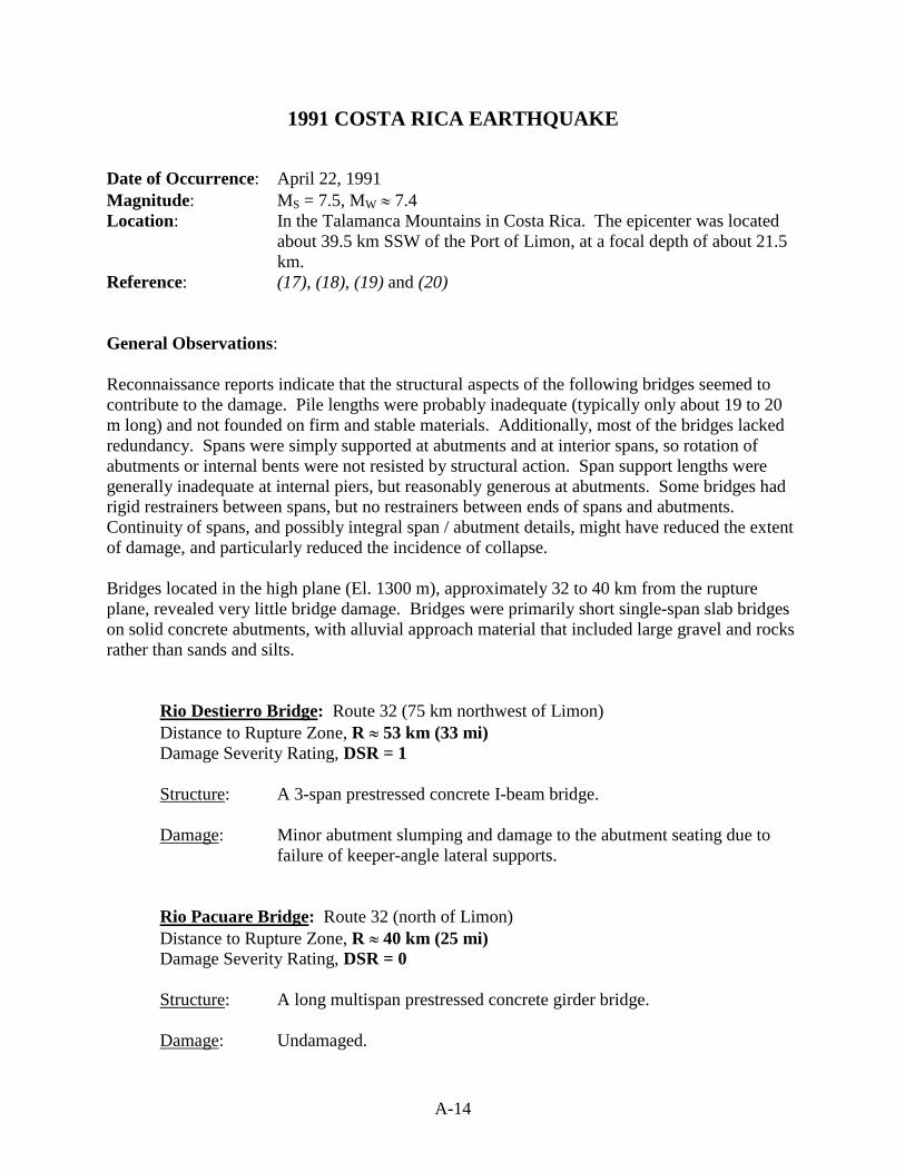
A-14

1991 COSTA RICA EARTHQUAKE

Date of Occurrence: April 22, 1991 Magnitude: MS = 7.5, MW � 7.4 Location: In the Talamanca Mountains in Costa Rica. The epicenter was located

about 39.5 km SSW of the Port of Limon, at a focal depth of about 21.5 km.

Reference: (17), (18), (19) and (20) General Observations: Reconnaissance reports indicate that the structural aspects of the following bridges seemed to contribute to the damage. Pile lengths were probably inadequate (typically only about 19 to 20 m long) and not founded on firm and stable materials. Additionally, most of the bridges lacked redundancy. Spans were simply supported at abutments and at interior spans, so rotation of abutments or internal bents were not resisted by structural action. Span support lengths were generally inadequate at internal piers, but reasonably generous at abutments. Some bridges had rigid restrainers between spans, but no restrainers between ends of spans and abutments. Continuity of spans, and possibly integral span / abutment details, might have reduced the extent of damage, and particularly reduced the incidence of collapse. Bridges located in the high plane (El. 1300 m), approximately 32 to 40 km from the rupture plane, revealed very little bridge damage. Bridges were primarily short single-span slab bridges on solid concrete abutments, with alluvial approach material that included large gravel and rocks rather than sands and silts.

Rio Destierro Bridge: Route 32 (75 km northwest of Limon) Distance to Rupture Zone, R � 53 km (33 mi) Damage Severity Rating, DSR = 1

Structure: A 3-span prestressed concrete I-beam bridge.

Damage: Minor abutment slumping and damage to the abutment seating due to

failure of keeper-angle lateral supports.

Rio Pacuare Bridge: Route 32 (north of Limon) Distance to Rupture Zone, R � 40 km (25 mi) Damage Severity Rating, DSR = 0

Structure: A long multispan prestressed concrete girder bridge.

Damage: Undamaged.

A-15

Rio Quebrada Calderon and Rio Aquas Claras Bridges: Rt 32 (40 km from Limon) Distance to Rupture Zone, R � 29 and 82 km (18 and 20 mi) Damage Severity Rating, DSR = 1

Structure: Both bridges were single span.

Damage: Extensive slumping of abutment fill material, but the use of settlement

slabs on the approaches of both bridges enabled them to remain serviceable.

Rio Chirripo Bridge: Route 32 (between San Jose and Limon) Distance to Rupture Zone, R � 23 km (14 mi) Damage Severity Rating, DSR = 3

Structure: Six-span continuous steel girder bridge with a short, 16 meter, simply

supported span at the end.

Damage: Short end span lost to liquefaction. The slab pier support at the end of the span rotated inwards, together with probable abutment movement.

Rio Buffalo Bridge: Route 32 (10 km from Limon) Distance to Rupture Zone, R � 21 km (13 mi) Severity Rating, DSR = 3

Structure: A 3-span prestressed concrete beam and slab bridge.

Damage: Abutment material failure with severe rotation of the abutments and

slumping of the bank material that exposed piles.

Rio Banano Bridge: Route 36 (south of Limon) Distance to Rupture Zone, R � 27 km (17 mi) Damage Severity Rating, DSR = 3

Structure: Single lane bridge consisting of three 22 m spans of twin prestressed

concrete I-beams with a shorter span at the north end. Piles are 36 cm2 precast concrete. Front piles are driven at a batter of 1:5.

Damage: Extensive signs of liquefaction were present. Soil movement caused

about 9� rotation of the south abutment resulting in a movement of the pile tops toward the river of about 66 cm. Front piles suffered flexural as well as shear failures. Vertical piles at rear showed less damage.

A-16

Comments: Near the bridge, a several hundred foot wide flood plain consisting of

sand and gravels liquefied and spread laterally towards the river on shallow slopes. The approach fills behind the southern embankment slumped, with some of the materials slipping towards the river through pile bents. The log of a boring drilled at the south abutment shows that the surficial sands and gravels are relatively thin and, in general, the piles are supported by silty and clayey materials.

Rio Viscaya Bridge: Route 36 (south of Limon) Distance to Rupture Zone, R � 27 km (17 mi) Damage Severity Rating. DSR = 3

Structure: A 3-span prestressed concrete I-beam bridge. Each span is simply supported on the abutments and/or interior piers.

Damage: Two spans lost due to severe abutment rotation, pile distress, and

collapse of one interior support. A second interior support settled vertically about 1 m. The south abutment rotated 8� and was pushed towards the center of the river. Hinge restrainers between the spans pulled out of the span end diaphragms. Total collapse of this structure might have been averted by a less articulated design.

Comments: The bridge was founded in soft sands, effectively on the shoreline, and

collapsed due to loss of support and ground deformations resulting from soil liquefaction. The log of a boring drilled near the north abutment shows that the entire length of piles is supported in sands and silty sands. Liquefaction soils in approach fills caused lateral spreading and bearing capacity failure. The north roadway approach fill settled approximately 120 cm. North and south abutment rotation was caused by movement of liquefied soils.

Rio Bananito Bridge: Route 36 (south of Limon) Distance to Rupture Zone, R � 27 km (17 mi) Damage Severity Rating, DSR = 3

Structure: A two span skewed prestressed concrete I-beam bridge. The bridge abutment and central slab pier were skewed at 30�.

Damage: Both spans were lost off the central pier, with the spans being thrown off

in the direction of the skew. Both abutments rotated towards the river at

A-17

the base. The southern abutment rotated about 15� due to lateral flow of the ground towards the river.

Comments: The road runs on a sand bar in the north and on a marsh in the south.

Many fissures parallel to the river were observed along the river bank and the approach roadway slumped.

Estero Negro Bridge: Route 36 (south of Limon) Distance to Rupture Zone, R � 27 km (17 mi) Damage Severity Rating, DSR = 3

Structure: Two span prestressed concrete I-beam bridge.

Damage: One span fell down. The lateral flow of the ground at the right river

bank pushed the abutment and the remaining span, which resulted in the falling down of the missing span.

Comments: There was another bridge crossing a small creek about 3 km south from

the Rio Estero Negro bridge. The approach roadway subsided but the bridge was not damaged.

Rio Estrella Bridge: Route 36 (south of Limon) Distance to Rupture Zone, R � 26 km (16 mi) Damage Severity Rating, DSR = 1

Structure: Bridge consisted of two 75 m steel truss spans, with a 25 m prestressed concrete I-girder span at the northern end.

Damage: Both truss spans fell off their supports. The south span fell off the south

abutment, and collapsed at the central abutment by fracture of the two bottom cords immediately adjacent to the central slab pier. The end diagonal buckled and the span dropped. The northern span pulled off the central support but was still supported at the northern end.

Comments: The roadway approach to the south abutment of the bridge, as well as the

banana plantations on both sides of the road, were dissected by several large and many small fissures indicative of liquefaction at depth and lateral spreading of surface flood-plain deposits toward the river channel. Lateral displacements were as large as 1 to 3 m based on open widths of fissures observed in the roadway and adjacent banana fields. The soil supporting the roadway at the south abutment compacted during the earthquake causing the approaching roadway to settle about 1.5 m. Roadway settlement near the north abutment was about 0.2 m. Only a

A-18

few longitudinal cracks developed in the pavement and approach fill; no open fissures were found in natural ground within several tens of meters of the north abutment.

Despite signs of large soil movements at the southern abutment, there were no signs of permanent deformation or rotation. An investigation was made where pertinent points on each abutment and pier were surveyed to determine post-earthquake distances between structural elements for comparison with distances noted on the bridge plans. The comparisons indicate very little displacement of the piers and abutments during the earthquake. The differences between plan and measured distances fall within the range of expected survey and construction error and indicate that no substantial permanent displacement occurred between these elements. The foundation for this abutment apparently was sufficiently strong to resist the lateral soil movement and hold the abutment in place.

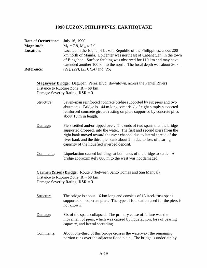
A-19

1990 LUZON, PHILIPPINES, EARTHQUAKE

Date of Occurrence: July 16, 1990 Magnitude: MS = 7.8, MW � 7.9 Location: Located in the Island of Luzon, Republic of the Philippines, about 200

km north of Manila. Epicenter was northeast of Cabanatuan, in the town of Bingabon. Surface faulting was observed for 110 km and may have extended another 100 km to the north. The focal depth was about 36 km.

Reference: (21), (22), (23), (24) and (25)

Magsaysay Bridge: Dagupan, Perez Blvd (downtown, across the Pantel River) Distance to Rupture Zone, R � 60 km Damage Severity Rating, DSR = 3

Structure: Seven-span reinforced concrete bridge supported by six piers and two

abutments. Bridge is 144 m long comprised of eight simply supported reinforced concrete girders resting on piers supported by concrete piles about 10 m in length.

Damage: Piers settled and/or tipped over. The ends of two spans that the bridge

supported dropped, into the water. The first and second piers from the right bank moved toward the river channel due to lateral spread of the river bank and the third pier sank about 2 m due to loss of bearing capacity of the liquefied riverbed deposit.

Comments: Liquefaction caused buildings at both ends of the bridge to settle. A

bridge approximately 800 m to the west was not damaged.

Carmen (Sison) Bridge: Route 3 (between Santo Tomas and San Manual) Distance to Rupture Zone, R � 60 km Damage Severity Rating, DSR = 3

Structure: The bridge is about 1.6 km long and consists of 13 steel-truss spans supported on concrete piers. The type of foundation used for the piers is not known.

Damage: Six of the spans collapsed. The primary cause of failure was the

movement of piers, which was caused by liquefaction, loss of bearing capacity, and lateral spreading.

Comments: About one-third of this bridge crosses the waterway; the remaining

portion runs over the adjacent flood plain. The bridge is underlain by

A-20

quaternary alluvial, lacustrine, beach, and residual deposits. Numerous large sand boils were seen in the area.

Cayanga Bridge: Coastal road south of Agoo Distance to Rupture Zone, R � 65 km Damage Severity Rating, DSR = 1

Structure: Long, “modern” bridge with concrete spans and piers.

Damage: The approach to the south abutment had settled, and there was extensive

cracking and subsidence in the soil adjacent to the abutment. Lateral spreading caused slight shifting in a support column and an offset in a bridge support pad.

Comments: Bridge was relatively undamaged, although there was significant lateral

spreading, and settlement of the soils and road bed adjacent to the south abutment.

A-21

1989 LOMA PRIETA EARTHQUAKE

Date of Occurrence: October 17, 1989 Magnitude: MW = 6.9, MS = 7.1 Location: The epicenter was located 16 km northeast of Santa Cruz and

approximately 30 km south of San Jose. The depth was approximately 18 km below the surface of the Earth.

Reference: (26) General Observations: Minor liquefaction, as evidenced by small sand boils, occurred beneath several elevated sections of the highway “distribution structure” immediately inland of the Bay Bridge approach fill. Several of these boils were adjacent to one of the elevated support bents in this area. The minor liquefaction does not appear to have resulted in any significant damage to the distribution structure. Within a few hundred yards of the destroyed Marine Research Facility, located on a sandy peninsula between the Pacific Ocean and the old trace of the Salinas River, an approach fill to a timber pile supported bridge across the old Salinas River was found to have slumped approximately 1 to 1.5 m, severing water and/or sewer pipe lines running across the bridge. General Damage to Bridge Structures: � Soquel Avenue Bridge in Santa Cruz (42).

Distance to Rupture Plane, R � 22 km (12 mi) Damage Severity Rating, DSR = 1

� Broadway Avenue Bridge in Santa Cruz (42).

Distance to Rupture Plane, R � 22 km (12 mi) Damage Severity Rating, DSR = 1

� Riverside Avenue Bridge in Santa Cruz (42).

Distance to Rupture Plane, R � 22 km (12 mi) Damage Severity Rating, DSR = 1

� Highway 1 Bridge at Moss Landing (42).

Distance to Rupture Plane, R � 22 km (12 mi) Damage Severity Rating, DSR = 1

A-22

� Highway 1 Bridge at Pajaro River (42).

Distance to Rupture Plane, R � 29 km (15.5 mi) Damage Severity Rating, DSR = 0

� Small wooden bridge at Moss Landing (42).

Distance to Rupture Plane, R � 22 km (12 mi) Damage Severity Rating, DSR = 1

� Corralitos Creek Bridge (42).

Distance to Rupture Plane, R � 11 km (6 mi) Damage Severity Rating, DSR = 1

� County Bridge near Salinas River (42).

Distance to Rupture Plane, R � 27 km (14.5 mi) Damage Severity Rating, DSR = 0

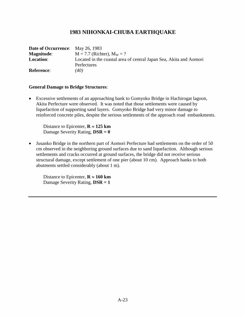
A-23

1983 NIHONKAI-CHUBA EARTHQUAKE

Date of Occurrence: May 26, 1983 Magnitude: M = 7.7 (Richter), MW = ? Location: Located in the coastal area of central Japan Sea, Akita and Aomori

Perfectures Reference: (40) General Damage to Bridge Structures: � Excessive settlements of an approaching bank to Gomyoko Bridge in Hachirogat lagoon,

Akita Perfecture were observed. It was noted that those settlements were caused by liquefaction of supporting sand layers. Gomyoko Bridge had very minor damage to reinforced concrete piles, despite the serious settlements of the approach road embankments.

Distance to Epicenter, R � 125 km Damage Severity Rating, DSR = 0

� Jusanko Bridge in the northern part of Aomori Perfecture had settlements on the order of 50

cm observed in the neighboring ground surfaces due to sand liquefaction. Although serious settlements and cracks occurred at ground surfaces, the bridge did not receive serious structural damage, except settlement of one pier (about 10 cm). Approach banks to both abutments settled considerably (about 1 m).

Distance to Epicenter, R � 160 km Damage Severity Rating, DSR = 1

A-24

1980 EL-ASNAM, ALGERIA, EARTHQUAKE

Date of Occurrence: October 10, 1980 Magnitude: MS = 7.3, M = 7.2 (Richter), MW � 7.2 Location: The epicenter was located approximately 10 km east of El-Asnam at a

focal depth of about 10 km. Reference: (27) General Observations: Most bridge abutments settled during the earthquake, thereby damaging bridge approaches. The differential settlement was jointly due to lurching, liquefaction, and uneven compaction.

Cheliff River Bridge: 15 km NE of El-Asnam and about 5 km SW of Beni Rached Distance to Rupture Zone, R � 5 to 10 km Damage Severity Rating, DSR = 1

Structure: Two-lane modern prestressed concrete bridge continuous over five

spans. Intermediate spans are supported on twin piers, the lower ends of which are protected from scour by a steel caisson lining.

Damage: Except for some cracking of concrete at the foundation in the steel

caisson, there was no evidence of structural damage to the spans, piers, or foundation. There was also no evidence of pier settlement. The only faulty detailing was at each end, where bearing beams that transferred the bridge load to the wing walls had moved. These bearing beams were keyed into the abutment approach structure but were not tied back; so in the case of the southern abutment, which had undergone a significant rigid body rotation, its bearing beam was almost lost. Relative movement to 1 m horizontally and 0.30 m vertically occurred between the approach and the deck.

Comments: Along the river in the neighborhood of the bridge, considerable land

movement and soil liquefaction were observed.

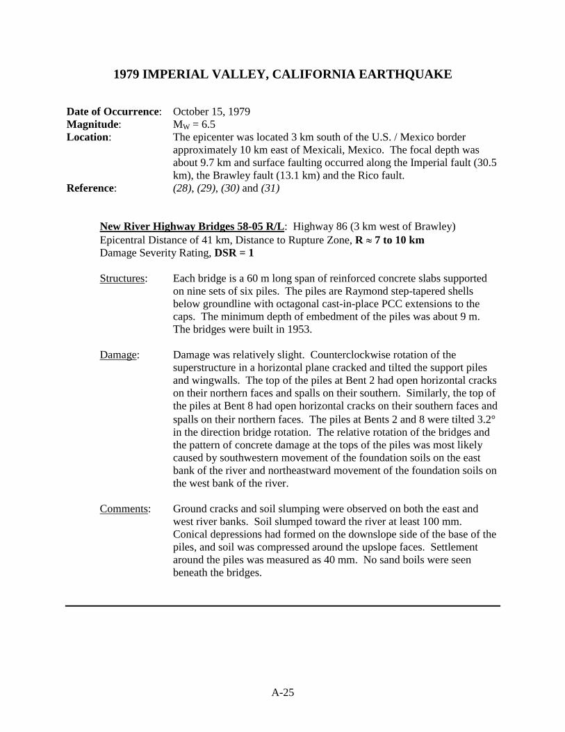
A-25

1979 IMPERIAL VALLEY, CALIFORNIA EARTHQUAKE

Date of Occurrence: October 15, 1979 Magnitude: MW = 6.5 Location: The epicenter was located 3 km south of the U.S. / Mexico border

approximately 10 km east of Mexicali, Mexico. The focal depth was about 9.7 km and surface faulting occurred along the Imperial fault (30.5 km), the Brawley fault (13.1 km) and the Rico fault.

Reference: (28), (29), (30) and (31)

New River Highway Bridges 58-05 R/L: Highway 86 (3 km west of Brawley) Epicentral Distance of 41 km, Distance to Rupture Zone, R � 7 to 10 km Damage Severity Rating, DSR = 1

Structures: Each bridge is a 60 m long span of reinforced concrete slabs supported

on nine sets of six piles. The piles are Raymond step-tapered shells below groundline with octagonal cast-in-place PCC extensions to the caps. The minimum depth of embedment of the piles was about 9 m. The bridges were built in 1953.

Damage: Damage was relatively slight. Counterclockwise rotation of the

superstructure in a horizontal plane cracked and tilted the support piles and wingwalls. The top of the piles at Bent 2 had open horizontal cracks on their northern faces and spalls on their southern. Similarly, the top of the piles at Bent 8 had open horizontal cracks on their southern faces and spalls on their northern faces. The piles at Bents 2 and 8 were tilted 3.2� in the direction bridge rotation. The relative rotation of the bridges and the pattern of concrete damage at the tops of the piles was most likely caused by southwestern movement of the foundation soils on the east bank of the river and northeastward movement of the foundation soils on the west bank of the river.

Comments: Ground cracks and soil slumping were observed on both the east and

west river banks. Soil slumped toward the river at least 100 mm. Conical depressions had formed on the downslope side of the base of the piles, and soil was compressed around the upslope faces. Settlement around the piles was measured as 40 mm. No sand boils were seen beneath the bridges.

A-26

1978 MIYAGI-KEN-OKI, JAPAN, EARTHQUAKE

Date of Occurrence: June 12, 1978 Magnitude: MS = 7.4, MW � 7.3 Location: The epicenter is located offshore Japan, approximately 115 km east of

Sendai, from a focal depth of about 60 km. Reference: (32), (33) and (40)

Yuriage Bridge: Located outside Sendai (1.2 km from the mouth of the Noatori River) Distance to Epicenter, R � 107 km Damage Severity Rating, DSR = 1

Structure: A 10-span bridge constructed in 1962. Seven prestressed-concrete T-

girders, each 45 m long, and three main spans. The spans are twin-cell, segmentally constructed, post-tensioned concrete box girders. The center span which is 90 m long, has a 60 m span at either end.

Damage: The bridge was open to only one lane of traffic because of heavy column

damage. No damage was reported to the three-span box structure. Light girder impacting with the abutment and pronounced shear cracking of the exterior girder at the bearing was evident. Pier 1, founded on a caisson 19 m deep and 2 m by 4 m in plan, suffered heavy shear cracking. The pier cap was reported to have settled 5 cm uniformly.

Comments: Liquefaction was evident in the flood plain below the bridge.

General Damage to Bridges Structures: � Abukuma Bridge, located on National Highway No. 6, sustained heavy cracks to several pier

columns. A sand boil was observed next to one the bridge piers.

Distance to Epicenter, R � 112 km Damage Severity Rating, DSR = 2

A-27

1976 MINDANAO, PHILIPPINES, EARTHQUAKE

Date of Occurrence: August 17, 1976 Magnitude: MS = 7.9, MW � 7.9 Location: The epicenter was located offshore in the Moro Gulf approximately 110

km south of Cotabato City and about 12 km west of Cadiz Point. Reference: (34) General Damage to Bridge Structures: Soil movements and failures were found at two bridges in Cotabato City. Abutment soil cracks were exhibited at the Quirino and Tamontaka Bridges. Notable ground cracking occurred to the west of the Quirino Bridge on both sides of the Rio Grande. Some of these ground cracks were 25 cm wide and 1.8 m deep, with as much as 25 cm of settlement on the river side. � The Quirino Bridge is a four span structural steel bridge. Each span of this bridge over the

Rio Grande de Mindanao River is 40 m long. The second span from the south end collapsed into the river during the earthquake. The northerly pier appeared to be leaning to the north. Two blocks west of the Quirino Bridge, observations were made of the ground sloughing in on both sides, toward the center of the river.

Distance to Epicenter, R � 110 km Damage Severity Rating, DSR = 1

� The Tamontaka Bridge is located approximately 6 km SSW of Central Cotabato City.

Spanning some 230 m across the Tamontaka River, the bridge is made up of six spans resting on pile supported piers. The 180 cm deep box girder sections, as well as piers and piles are reinforced concrete. Most of the damage to this bridge appears to be related to inertial effects. One exception is the movement of the abutments. Soft, swampy land surrounds the bridge. Displacement was visible between the roadway and its apron, north of the bridge. Displacements on the north end of the bridge on the order of 46 cm, sheared a 26 cm cast iron water supply pipe.

Distance to Epicenter, R � 104 km Damage Severity Rating, DSR = 1

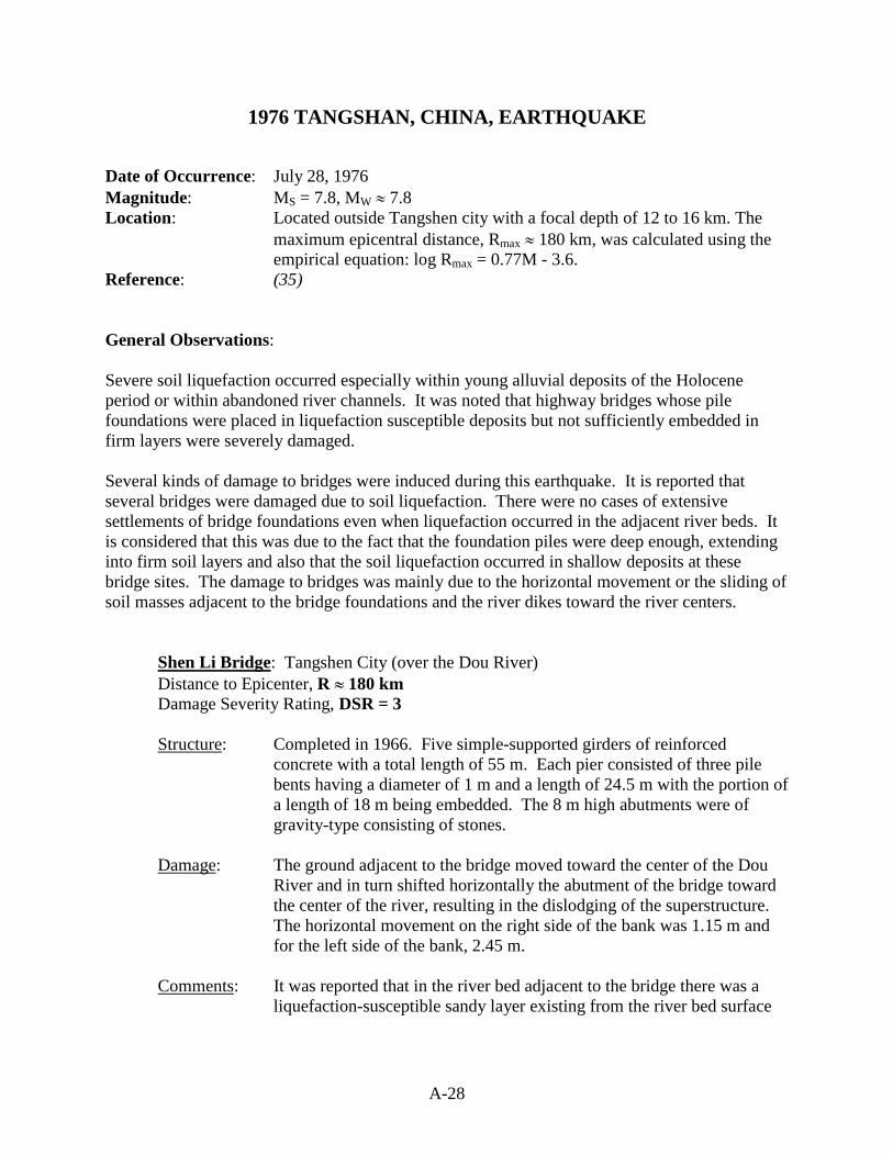
A-28

1976 TANGSHAN, CHINA, EARTHQUAKE

Date of Occurrence: July 28, 1976 Magnitude: MS = 7.8, MW � 7.8 Location: Located outside Tangshen city with a focal depth of 12 to 16 km. The

maximum epicentral distance, Rmax � 180 km, was calculated using the empirical equation: log Rmax = 0.77M - 3.6.

Reference: (35) General Observations: Severe soil liquefaction occurred especially within young alluvial deposits of the Holocene period or within abandoned river channels. It was noted that highway bridges whose pile foundations were placed in liquefaction susceptible deposits but not sufficiently embedded in firm layers were severely damaged. Several kinds of damage to bridges were induced during this earthquake. It is reported that several bridges were damaged due to soil liquefaction. There were no cases of extensive settlements of bridge foundations even when liquefaction occurred in the adjacent river beds. It is considered that this was due to the fact that the foundation piles were deep enough, extending into firm soil layers and also that the soil liquefaction occurred in shallow deposits at these bridge sites. The damage to bridges was mainly due to the horizontal movement or the sliding of soil masses adjacent to the bridge foundations and the river dikes toward the river centers.

Shen Li Bridge: Tangshen City (over the Dou River) Distance to Epicenter, R � 180 km Damage Severity Rating, DSR = 3

Structure: Completed in 1966. Five simple-supported girders of reinforced

concrete with a total length of 55 m. Each pier consisted of three pile bents having a diameter of 1 m and a length of 24.5 m with the portion of a length of 18 m being embedded. The 8 m high abutments were of gravity-type consisting of stones.

Damage: The ground adjacent to the bridge moved toward the center of the Dou

River and in turn shifted horizontally the abutment of the bridge toward the center of the river, resulting in the dislodging of the superstructure. The horizontal movement on the right side of the bank was 1.15 m and for the left side of the bank, 2.45 m.

Comments: It was reported that in the river bed adjacent to the bridge there was a

liquefaction-susceptible sandy layer existing from the river bed surface

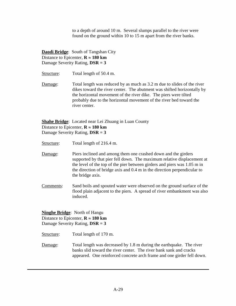
A-29

to a depth of around 10 m. Several slumps parallel to the river were found on the ground within 10 to 15 m apart from the river banks.

Daodi Bridge: South of Tangshan City Distance to Epicenter, R � 180 km Damage Severity Rating, DSR = 3

Structure: Total length of 50.4 m.

Damage: Total length was reduced by as much as 3.2 m due to slides of the river

dikes toward the river center. The abutment was shifted horizontally by the horizontal movement of the river dike. The piers were tilted probably due to the horizontal movement of the river bed toward the river center.

Shahe Bridge: Located near Lei Zhuang in Luan County Distance to Epicenter, R � 180 km Damage Severity Rating, DSR = 3

Structure: Total length of 216.4 m.

Damage: Piers inclined and among them one crashed down and the girders

supported by that pier fell down. The maximum relative displacement at the level of the top of the pier between girders and piers was 1.05 m in the direction of bridge axis and 0.4 m in the direction perpendicular to the bridge axis.

Comments: Sand boils and spouted water were observed on the ground surface of the

flood plain adjacent to the piers. A spread of river embankment was also induced.

Ninghe Bridge: North of Hangu Distance to Epicenter, R � 180 km Damage Severity Rating, DSR = 3

Structure: Total length of 170 m.

Damage: Total length was decreased by 1.8 m during the earthquake. The river

banks slid toward the river center. The river bank sank and cracks appeared. One reinforced concrete arch frame and one girder fell down.

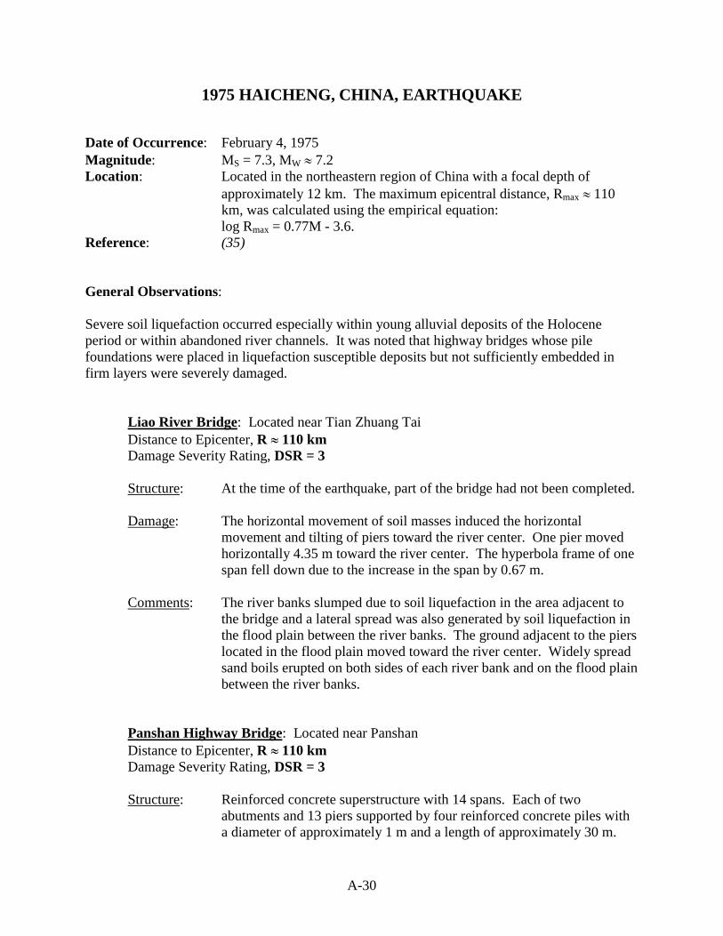
A-30

1975 HAICHENG, CHINA, EARTHQUAKE

Date of Occurrence: February 4, 1975 Magnitude: MS = 7.3, MW � 7.2 Location: Located in the northeastern region of China with a focal depth of

approximately 12 km. The maximum epicentral distance, Rmax � 110 km, was calculated using the empirical equation:

log Rmax = 0.77M - 3.6. Reference: (35) General Observations: Severe soil liquefaction occurred especially within young alluvial deposits of the Holocene period or within abandoned river channels. It was noted that highway bridges whose pile foundations were placed in liquefaction susceptible deposits but not sufficiently embedded in firm layers were severely damaged.

Liao River Bridge: Located near Tian Zhuang Tai Distance to Epicenter, R � 110 km Damage Severity Rating, DSR = 3

Structure: At the time of the earthquake, part of the bridge had not been completed.

Damage: The horizontal movement of soil masses induced the horizontal

movement and tilting of piers toward the river center. One pier moved horizontally 4.35 m toward the river center. The hyperbola frame of one span fell down due to the increase in the span by 0.67 m.

Comments: The river banks slumped due to soil liquefaction in the area adjacent to

the bridge and a lateral spread was also generated by soil liquefaction in the flood plain between the river banks. The ground adjacent to the piers located in the flood plain moved toward the river center. Widely spread sand boils erupted on both sides of each river bank and on the flood plain between the river banks.

Panshan Highway Bridge: Located near Panshan Distance to Epicenter, R � 110 km Damage Severity Rating, DSR = 3

Structure: Reinforced concrete superstructure with 14 spans. Each of two

abutments and 13 piers supported by four reinforced concrete piles with a diameter of approximately 1 m and a length of approximately 30 m.

A-31

Damage: One pier (No. 7) sank 15 cm. Other piers inclined and cracks were

induced in these piers. During a major aftershock (MS = 5), pier No. 7 sank again and four superstructure spans fell. Also during the aftershock, the tops of some piers inclined to the river bank due to the ground movement toward the river center.

A-32

1968 EBINO EARTHQUAKE

Date of Occurrence: February 21, 1968 Magnitude: M = 6.1 (Richter), MW � 6.1 Location: Ebino, Nishimoro-kata County, southern part of Kyushu Island, with a

very shallow hypocenter Reference: (41)

Ikejima Bridge: Ebino municipal road across the Ikejima River Distance to Epicenter, R � 10 km Damage Severity Rating, DSR = 1

Structure: Abutments and two piers are of solid-slab-type reinforced concrete

structures with spread footings and wooden pile foundations. The superstructure is of 3-span steel H-shaped simple girders.

Damage: A pier on the left bank settled about 25 cm. Evidence of liquefaction

was noted in the general area.

A-33

1964 ALASKA EARTHQUAKE

Date of Occurrence: March 27, 1964 Magnitude: MW = 9.2 Location: The epicenter was located in the Chugach Mountains near the northern

end of Prince Williams Sound about 130 km east-southeast of Anchorage. The depth to hypocenter was approximated to be 20 to 50 km.

Reference: (20), (28), (36) and (37) General Observations: A wealth of information is available on these bridges and the soils they were founded on. Foundation displacements for over 160 bridges were classified with varying degrees of severity. Approximate distances of the damage locations from the zone of major energy release range from 80 to 150 km (see table below). The proximity of damage locations to the energy-release zone is therefore not likely to be a significant factor is determining the relative damage at the various locations or in adjacent areas. Variations in bridge behavior are more likely to be due to differences in type of superstructure, type of foundation, foundation-soil conditions, and local topography. Table A.2: Estimated Distances from Zone of Major Energy Release to Bridge Damage Locations

GENERAL LOCATION APPROXIMATE DISTANCE FROM ZONE OF MAJOR ENERGY RELEASE

Resurrection River 111 km (60 miles) Snow River 111 km (60 miles)

Kenai River (Sterling Highway) 148 km (80 miles) Turnagain Arm (Portage Area) 93 km (50 miles)

Scott Glacier Streams 93 km (50 miles) Sheridan Glacier Streams 102 km (55 miles)

Lower Copper River 130 km (70 miles) Instead of looking at each specific bridge and its associated damage, some of the insights that were gained from the examination of such a large bridge sampling are presented: � No cases of evident foundation displacement were reported for bridges known to be founded

wholly on bedrock. � The greatest concentrations of bridges that sustained severe foundation movements were

founded on piling driven through saturated sands and silts of low-to-medium relative density (N<20).

A-34

� Bridges founded on piles that were driven through loose to medium-dense sands and silts into

denser sands and silts fared better than those founded on piles that were embedded in loose to medium-dense sand and silt without reaching denser strata. The mode of failure may have been different in these two support conditions, but severe foundation displacements occurred in both.

� Bridge foundations that were founded in gravels and gravelly sands (regardless of N values),

rather than in sands and silts, behaved relatively well. � Severe foundation displacements in sands and silts had foundations ranging from light

flexible all-timber bents through steel-rail and concrete bents to heavy reinforced-concrete piers with four-way-battered concrete-filled steel-tube piles extending to a total depth of about 30.4 m (100 ft).

� No failures of bridges founded in cohesive soils had been reported along the highways

investigated. � Bridge-foundation damage included horizontal movement of abutment foundations toward

the channels, spreading and settlement of abutment fills, horizontal displacement and tilting of piers, severe differential settlement of abutments and piers, and failure of foundation members.

� The severity of damage to bridge foundations was dependent to a great extent on the

foundation-support conditions. � The greatest concentrations of severe damage occurred in regions characterized by thick

deposits of saturated cohesionless soils. Ample evidence exists of liquefaction of these materials during the earthquake.

� Bridges founded in saturated sands and silts sustained severe displacement of pile-supported

foundations even where the average penetration resistance of the upper 9 m (30 ft) of the soil was as high as 25 blows/ft. The degree of damage sustained by these bridges did not appear to be greatly influenced by an increase in density of the foundation soil at the pile tips and below.

A-35

1964 NIIGATA, JAPAN, EARTHQUAKE

Date of Occurrence: June 16, 1964 Magnitude: MS = 7.5, MW � 7.3 Location: The epicenter was near Awa Island in the Japan Sea, 22 km off the coast

of Japan. The focus of the earthquake was about 40 km deep. Reference: (22) General Observations: Permanent ground displacements resulting from liquefaction in Niigata City were quite large. Horizontal displacement measurements were made using aerial photographs and are provided on pages 3.11 to 3.15 (22). It is notable that the horizontal displacements in the vicinity of the Bandai, Yachiyo, and Showa Bridge abutments were reduced because of the resistance of the structures to ground displacements. Soil data, including cross sections, blow counts, and estimated liquefied layer is also available for the following bridges in the reference above. Generally, liquefaction was estimated to have occurred in the riverbed as well as in the ground on both banks.

Yachiyo Bridge: Niigata City Distance to Epicenter, R � 55 km Damage Severity Rating, DSR = 3

Structure: Foundations of the abutments and piers had been constructed on

reinforced concrete piles with a diameter of 300 mm and a length of about 10 m.

Damage: Piles extracted and examined after the earthquake showed that the piles

were severely destroyed at a depth of about 8 m from the top of the pile, and horizontal cracks, which could have been caused by the large bending moments were found through the piles. The permanent ground displacement on both banks were 4 to 6 m toward the river. The reason for pier failures can be conjectured as follows: the foundation of the piers were pushed toward the river due to large ground displacements while displacements at the top of the piers were restrained because of the resistance of the girders. This caused a large stress concentration in the center of the pier.

Showa Bridge: Niigata City Distance to Epicenter, R � 55 km Damage Severity Rating, DSR = 3

A-36

Structure: Modern bridge with 12 simply supported steel girders. Piers were

constructed by driving steel pipe piles, which had considerable flexibility in the direction of the bridge longitudinal axis.

Damage: Five girders fell into the water. Permanent ground displacement on the

left bank reached several meters, substantially deforming the foundation piles and causing the girders to fall.

A-37

1948 FUKUI, JAPAN, EARTHQUAKE

Date of Occurrence: June 28, 1948 Magnitude: MS = 7.1, MW � 6.9 Location: The epicenter was located below the eastern part of the Fukui Plain,

about 10 km northeast of Fukui City. The focal depth was approximately 30 km.

Reference: (22) and (41)

Nagaya Bridge: Tajima River Area Distance to Epicenter, R � 2 km Damage Severity Rating, DSR = 3

Structure: Eight spans of reinforced-concrete I-beams with a total length over 58.5

m, supported on concrete piers.

Damage: Three piers sank to ground level due to liquefaction and the beams fell to the ground.

Itagaki Bridge: Hashidate-Fukui Route, across the Ashiba River Distance to Epicenter, R � 10 km Damage Severity Rating, DSR = 3

Structure: Gravity-type reinforced concrete abutments with twelve reinforced

concrete rigid frame piers and caisson foundations. The superstructure consisted of 13-spans of reinforced concrete T-shaped girders.

Damage: Several of the piers tilted 1 to 12°. Eight spans fell into the river due to

the tilting of the piers. Both abutments had heavy cracks on the parapet walls and the wing masonry.

Shioya Bridge: Near the mouth of the Daishoji River Distance to Epicenter, R � 15 km Damage Severity Rating, DSR = 2

Structure: Concrete abutments and seven reinforced concrete rigid frame piers.

The superstructure consisted of 8-span I-shaped steel girders.

Damage: Abutments tilted slightly. Every pier tilted toward the left bank and settled. The maximum settlement was 25 cm at the second pier from the left bank.

A-38

Nagaune Bridge: Tajima River Area Distance to Epicenter, R � 4 km Damage Severity Rating, DSR = 3

Structure: Eight spans of wooden beams supported upon timber piers with concrete

foundations and a total length of 72.2 m.

Damage: Several piers sank due to loss of bearing capacity on the foundation soils as a result of liquefaction. Two piers in particular sank almost to ground level.

Comments: Both the Nagaya and Nagaune Bridges crossed the Tajima River and its

tributary, respectively. It was reported that numerous sand and water boils were observed during the earthquake.

Nakatzuno Bridge: Main Channel Area of Kuzurya River Distance to Epicenter, R � 8 km Damage Severity Rating, DSR = 3

Structure: The bridge consisted of 14 spans of I-shaped steel girders with a total

length of 259 m. The piers were reinforced concrete columns on open caisson foundations.

Damage: The piers sank, tilted substantially, and collapsed, and the simply-

supported girders fell. It was reported that damage to the collapsed girders was comparatively light in spite of the extensive damage to the piers.

A-39

1923 KANTO, JAPAN, EARTHQUAKE

Date of Occurrence: September 1, 1923 Magnitude: MS = 7.1, MW = 6.9 Location: The epicenter was in the Sagami Bay Reference: (22) and (41)

Banyu Bridge: National Route 1, Chigaski City (over Sagami River) Distance to Rupture Zone, R � 50 km Damage Severity Rating, DSR = 3

Structure: Under construction. No superstructure. Open caissons and abutments.

Damage: Open caissons leaned, rose buoyantly, and were displaced. Abutments

on both banks tilted toward the river. The inclination of the abutments was about 4� and 12� for the left and right banks, respectively. The damage to the bridge indicates that ground displacement occurred in a direction towards the Sagami River in addition to the displacement towards Okawa Creek.

Comments: This area is located on the left bank of the lower reaches of the Sagami

River. The geomorphilogical features of the Nakajima area are characterized by abandoned braided channels and abandoned channel bars. These channels and bars are covered with alluvial fan deposits. Liquefaction was very prevalent in this area (110 documented cases) with numerous large ground cracks and flooding due to the water “spurting” from the ground.

Arakawa Canal Bridge: Furu-Sumida Creek Area in Tokyo Distance to Rupture Zone, R � 80 km Damage Severity Rating, DSR = 3

Structure: Undetermined

Damage: The abutments settled about 0.9 m on the right bank and 1.2 m on the left

bank. A pier on the west bank side was displaced in the downstream direction. The movement of the pier might be a result of the movements in the direction of the Furu-Sumida Creek.

Comments: This area is generally a deltaic zone transitioned to a natural levee zone

of the Kanto Plain.

A-40

Tsurono-bashi Bridge: Bandaicho-Horaicho Road in Yokohama Distance to Rupture Zone, R � 40 km Damage Severity Rating, DSR = 2

Structure: This bridge, completed in 1914, had brick masonry abutments with

concrete foundations. Each of two piers were made of four spiral single-row cast iron pipe piles with some bracing. The superstructure consisted of 3-span simple steel plate girders.

Damage: Both abutments moved and tilted toward the center of the river, and two

piers tilted considerably toward the left bank. The superstructure moved largely toward the left bank.

Toyokuni Bridge: Located between Horai-cho and Masago-cho, over the Oala River Distance to Rupture Zone, R � 40 km Damage Severity Rating, DSR = 3

Structure: Three span, simple steel pony trusses reconstructed in 1897. Abutments

and two piers were made of masonry structures with concrete fill inside.

Damage: Considerable substructure movement and one end of a truss fell into the river. Both abutments moved toward the center of the river, and tilted in the direction of their backfill. Two piers tilted considerably toward the center of the river, with an angle of inclination of over 8� at the northern pier and 2° at the southern pier.

A-41

1906 SAN FRANCISCO EARTHQUAKE

Date of Occurrence: April 18, 1906 Magnitude: MW = 7.9 Location: The rupture was along 435 km (270 mi) of the San Andreas Fault. The

largest displacement being 6.4 m (21 ft) approximately 48 km (30 mi) northwest of San Francisco.

Reference: (20), (38) and (39)

Salinas River Bridge: Highway Bridge (south of Salinas, CA) Distance to Rupture Zone, R � 29 km (16 mi) Damage Severity Rating, DSR = 3

Structure: A large trussed structure in two spans and plank deck. The south pier

consisted of 26 piles and was incased in planking.

Damage: Lateral displacement of the floodplain physically displaced both ground and pile foundation about 1.8 m northward toward the river channel. The bridge trusses and deck were strong enough to remain intact and were essentially undamaged. The deck, which remained attached to the tops of the piers, acted as a strut, holding the tops of the piers in place while their bases shifted riverward. This motion left the southern pier inclined, with the top of the pier tilted outward, away from the river (20). Additional information can be found on page 292, (38) and page 13, (39).

General Damage to Bridge Structures: � On the east bank of the main Eal River, to the east of Laytonville, the ground was cracked for

a distance of 274 m (300 yd), the trend of the crack following the course of the river. The crack was merely local in the alluvial bank of the stream, perhaps 91.5 m (100 yd) from the water. A long bridge crossing the stream at this place showed no damage (38, pg 170; 39, pg 165).

Distance to San Andreas Fault, R � 57 km (31 mi) Damage Severity Rating, DSR = 0

� A railroad bridge across a lagoon in Cleone, Mendcino County, sank 1 m (3 ft) in some

places, and was thrown out of line laterally, all the piling supporting the bridge were listed to the south (38, pg 172; 39, pg 165).

Distance to San Andreas Fault, R � 5.5 km (3 mi) Damage Severity Rating, DSR = 3

A-42

� In Mendocino, Mendocino County, the bridge over the Big River was severely damaged. A short span in the long approach on the north side entirely collapsed. The fall of the span was due to the shifting north of piles on the north side of the river, thus allowing one end to drop (38, pg 175).

Distance to San Andreas Fault, R � 5.5 km (3 mi) Damage Severity Rating, DSR = 3

� An old bridge in Alexander Valley, east of Layton Springs, was wrecked, “the trestle-work

art going down.” There was evidence of liquefaction in the general vicinity (38, pg 184; 39, pg 160).

Distance to San Andreas Fault, R � 29 km (16 mi) Damage Severity Rating, DSR = 3

� It was noted that the “fills” in Tomales Bay generally sank from 0.6 to 2.5 m (2 to 8 ft). In a

couple instances the pile-supported bridge in the middle of the fill remained at grade. Just above Hamlet a trestle-work which had been filled in settled, leaving the trestle-work some 0.6 m (2 ft) above. The bottom of the bay in these arms is usually sand (38, pg 197; 39, pg 152). Indications are of little damage to trestles.

Distance to San Andreas Fault, R � 3.7 km (2 mi) Damage Severity Rating, DSR = 3

� Portions of the trestle over Launitas Creek, about 1.6 km (1 mi) form Point Reyes, were

thrown entirely off the piles, the piles themselves being moved downstream (39, pg 152).

Distance to San Andreas Fault, R � 3.7 km (2 mi) Damage Severity Rating, DSR = 3

� At the Southern Pacific Bridge, crossing the San Lorenzo River, there is a network of fissures

varying from 50 to 380 mm (2 to 15 in) in width, running thru the sandy soil. The direction of the main fissures is east and west, and they are on the south side of the river, which is nearest the Bay. The ground has settled about 250 mm (10 in) from the abutments and piers of the bridge (39, pg 87).

Distance to San Andreas Fault, R � 26 km (14 mi) Damage Severity Rating, DSR = 0

� A railroad bridge at Lake Merced, about 9.5 km (6 mi) north of Mussel Rock was badly

wrecked. Both lateral and vertical movements were extremely large, 1.5 to 4.5 m (5 to 15 ft). Evidence of liquefaction in the form of sand boils were found in the general vicinity (38, pg 251).

Distance to San Andreas Fault, R � 5.5 km (3 mi) Damage Severity Rating, DSR = 3

A-43

� The bridge over Coyote Creek, on the Alviso-Milipitas road was severely damaged by

liquefaction and lateral spreading. The concrete abutments were thrust inward toward each other about 0.9 m (3 ft). A pile driven in the middle of the stream, which had been cut off below water level, was lifted about 0.6 m (2 ft) (38, pg 281; 39, pg 113). The entire area was the location of large fissures, sand boils, and lateral streamward movements occurring as a result of liquefaction. It was also noted that another bridge crossing the Coyote Creek experienced little damage, only small movements. There is no mention of any soil failures in the area of this other (southern) bridge (38, pg 280).

Distance to San Andreas Fault (northern bridge), R � 28 km (15 mi) Damage Severity Rating, DSR = 3

� Two bridges located at Neponset over the Salinas River were damaged. The northern

concrete piers of the railway bridge moved 51 mm (2 in) east, and the central wooden pier of the county bridge moved about 1.2 m (4 ft) south. Many mentions of liquefaction induced sand boils and fissures are made (38, pg 293; 39, pg 79).

Distance to San Andreas Fault, R � 26 km (14 mi) Damage Severity Rating (concrete railway pier), DSR = 1 Distance to San Andreas Fault, R � 26 km (14 mi) Damage Severity Rating (wooden central pile), DSR = 3

� At Neponset and Salinas the piling under the county bridges was moved in some bents as

least 10 feet toward the river. Large sand boils were observed in the area (38, pg 293).

Distance to San Andreas Fault, R � 26 km (14 mi) Damage Severity Rating, DSR = 3

� A county road bridge over the Pajaro River near Chittenden was severely damaged by lateral

spreading of sediments toward the river channel. The abutment was displaced and fractured. The damage to the concrete abutments of the county bridge across the Pajaro River is due to this crowding in of the alluvial banks of the stream. (39, pgs 22 & 85).

Distance to San Andreas Fault, R � 1.9 km (1 mi) Damage Severity Rating, DSR = 3

� The Southern Pacific Bridge across the Pajaro River, at Watsonville, consisted of four 80-ft

wooden spans on pile piers, had the second pier from the east end moved up steam about 3 feet. The highway bridge at Watsonville was distorted in similar manner to the Salinas Bridge described above due to the shifting of the bank deposits (39, pg 83).

Distance to San Andreas Fault (Southern Pacific Bridge), R � 12 km (6.5 mi) Damage Severity Rating, DSR = 3 Distance to San Andreas Fault (Highway Bridge), R � 12 km (6.5 mi) Damage Severity Rating, DSR = 3

A-44

� At Port Kenyon, a large field bordering Salt River was spread open in many places, several

acres of the land settling a couple feet. From its appearance it would seem that water spurted in large quantities from the ground. On the north bank of Salt River at the lower bridge the land has slid in and cracked for a distance of several hundred feet and a width of thirty to forty feet. The bridge itself does not seem to have been damaged any and is presumably in as good condition for travel as before the shock (39, pg 170).

Distance to San Andreas Fault, R � ? miles Damage Severity Rating, DSR = 0

� The bridges over the Russian River, at Healdsburg, and at Bohemia, on the California

Northwestern, were both shifted slightly on the piers at one end (39, pg 160).

Distance to San Andreas Fault (Healdsburg), R � 35 km (19 mi) Damage Severity Rating, DSR = 1 Distance to San Andreas Fault (Bohemia), R � 13 km (7 mi) Damage Severity Rating, DSR = 1

� The movement at Gonzales Bridge was mostly on the west Bank of the stream. Wooden

piles at the southwest end of the bridge, said to be driven down 22.8 m (75 ft), have been torn loose and moved from plumb. At the northeast end of the bridge the piles are undisturbed, but the surface soil has moved relatively 450 mm (18 in) northward (38, pg 293; 39, pg 75).

Distance to San Andreas Fault (SE extent of rupture), R � 44.5 km (24 mi) Damage Severity Rating, DSR = 2

A-45

1886 CHARLESTON, SOUTH CAROLINA, EARTHQUAKE

Date of Occurrence: Magnitude: MW = ? Location: Reference: (20) General Damage to Bridge Structures: � A Bridge over the Ashley River was damaged. Ground displacements as great as several

tenths of a meter shifted abutments and piers toward the centers of the channels, compressing bridge decks with attendant bulging up of stringers and overlapping of planks. Documented ground disturbances including ground fissures and sand boils confirm that liquefaction was widespread near these bridges.

Distance to Rupture Zone, R � ? Damage Severity Rating, DSR = 3

A-46

REFERENCES (1) Earthquake Engineering Research Institute (EERI) Newsletter (1995), December Vol. 29,

No. 12, ? p. (2) Japanese Geotechnical Society (1996). Special Issue on Geotechnical Aspects of the

January 17, 1995 Hyogoken-Nambu Earthquake, Soils and Foundations, 358 p. (3) Shinosuka, M., editor (1995). The Hanshin-Awaji Earthquake of January 17, 1995

Performance of Lifelines, Technical Report NCEER-95-0015, State University of New York at Buffalo, 270 p.

(4) Comartin, C.D., Greene, M., and Tubbesing, S.K., editors (1995). The Hyogo-Ken

Nanbu Earthquake, Preliminary Reconnaissance Report, Earthquake Engineering Research Institute (EERI) Report, 115 p.

(5) EQE International (1995). The January 17, 1995 Kobe Earthquake, An EQE Summary

Report, EQE International Publication, 94 p. (6) Stewart, J.P., Bray, J.D., Seed, R.B., and Sitar, N. (1994). Preliminary Report on the

Principle Geotechnical Aspects of the January 17, 1994 Northridge Earthquake, Report No. UCB/EERC-94/08, University of California at Berkeley, 245 p.

(7) Moehle, J.P., editor (1995). Northridge Earthquake Reconnaissance Report, Vol. 1,

Earthquake Spectra, EERI, Supplement C, Vol. 11, 521 p. (8) Earthquake Engineering Research Institute (EERI) Newsletter (1995), January Vol. 29,

No. 1, 6 p. (9) Swan, S.W., and Harris, S.K. (1993). The Island of Guam Earthquake of August 8, 1993,

Technical Report NCEER-93-0017, State University of New York at Buffalo, 34 p. (10) Comartin, C.D., editor (1995). Guam Earthquake Reconnaissance Report, Earthquake

Spectra, EERI, Supplement B, Vol. 11, 175 p. (11) Yanev, P.I., and Scawthorn, C.R. (1993). Hokkaido Nansei-oki Earthquake of July 12,

1993, Technical Report NCEER-93-0023, State University of New York at Buffalo, 110 p.

(12) Iwatate, T., Sawada, Y., Inoue, D., and Sakamoto, Y. (1994). “Characteristics and

Damage Investigation of 1993 Hokkaido Nansei-oki Earthquake,” Proceedings, Fifth U.S.-Japan Workshop on Earthquake Resistant Design of Lifeline Facilities and Countermeasures Against Soil Liquefaction, Technical Report NCEER-94-0026, State University of New York at Buffalo, pp 101-116.

A-47

(13) Isoyama, R. (1994). “Liquefaction-induced Ground Failures and Displacements along the Shiribeshi-toshibetsu River Caused by the 1993 Hokkaido-nansei-oki Earthquake,” Proceedings, Fifth U.S.-Japan Workshop on Earthquake Resistant Design of Lifeline Facilities and Countermeasures Against Soil Liquefaction, Technical Report NCEER-94-0026, State University of New York at Buffalo, pp 1-26.

(14) Moehle, J.P., editor (1995). Hokkaido Earthquake Reconnaissance Report, Earthquake

Spectra, EERI, Supplement A, Vol. 11, 166 p. (15) Beavers, J.E., editor (1993). Erzincan, Turkey Reconnaissance Report, Earthquake

Spectra, EERI, Supplement A, Vol. 9, 210 p. (16) Aydan, O., and Hamada, M. (1992). "An Investigation into the Erzincan (Turkey)

Earthquake of March 13, 1992," Proceedings, Fourth Japan-U.S. Workshop on Earthquake Resistant Design of Lifeline Facilities and Countermeasures for Soil Liquefaction, Technical Report NCEER-92-0019, State University of New York at Buffalo, Vol. I, pp 17-34.

(17) Beavers, J.E., editor (1991). Costa Rica Earthquake Reconnaissance Report,

Earthquake Spectra, EERI, Supplement B, Vol. 7, 127 p. (18) Yoshida, N., Watanabe, H., Yasuda, S., and Mora, S. (1992). “Liquefaction-induced

Ground Failure and Related Damage to Structures During 1991 Telire-Limon, Costa Rica, Earthquake,” Proceedings, Fourth Japan-U.S. Workshop on Earthquake Resistant Design of Lifeline Facilities and Countermeasures for Soil Liquefaction, Technical Report NCEER-92-0019, State University of New York at Buffalo, Vol. I, pp 37-52.

(19) Youd, T.L., Rollins, K.M., Salazar, A.F., and Wallace, R.M. (1992). “Bridge Damage

caused by liquefaction during the 22 April 1991 Costa Rica earthquake,” Proceedings, Tenth World Conference on Earthquake Engineering, Madrid, Spain, Vol. 1, pp 153-158.

(20) Youd, T.L. (1993). “Liquefaction-Induced Damage to Bridges,” Transportation

Research Record Report No. 1411, Earthquake-Induced Ground Failure Hazards, National Research Council, pp 35-41.

(21) Beavers, J.E., and Martin Marietta Energy Systems, editors (1991). Philippines

Earthquake Reconnaissance Report, Earthquake Spectra, EERI, Supplement A, Vol. 7, 144 p.

(22) Hamada, M., and O'Rourke, T.D., editors (1992). Case Studies of Liquefaction and

Lifeline Performance During Past Earthquakes, Technical Report NCEER-92-0001, State University of New York at Buffalo, Vol. 1, 341 p.

A-48

(23) Ishihara, K., Acacio, A.A., and Towhata, I. (1993). “Liquefaction-induced Ground Damage in Daugupan in the July 16, 1990 Luzon Earthquake,” Soils and Foundations, Vol. 33, No. 1, pp 133-154.

(24) Wakamatsu, K., Hamada, M., Tazoh, T., Yoshida, N., and Ando, T. (1991).

“Liquefaction-induced Ground Failure During the 1990 Philippines Earthquake,” Proceedings, Third Japan-U.S. Workshop on Earthquake Resistant Design of Lifeline Facilities and Countermeasures for Soil Liquefaction, Technical Report NCEER-91-0001, State University of New York at Buffalo, pp 23-27.

(25) Wieczorek, G.F., Arboleda, R., and Tubianosa, B. (1991). “Liquefaction and Landsliding

from the July 16, 1990, Luzon Philippines Earthquake,” Proceedings, Third Japan-U.S. Workshop on Earthquake Resistant Design of Lifeline Facilities and Countermeasures for Soil Liquefaction, Technical Report NCEER-91-0001, State University of New York at Buffalo, pp 39-55.

(26) Seed, R.B., Dickenson, S.E., Riemer, M.F., Bray, J.D., Sitar, N., Mitchell, J.K., Idriss,

I.M., Kayen, R.E., Kropp, A., Harder Jr., L.F., and Power, M.S. (1990). Preliminary Report on the Principle Geotechnical Aspects of the October 17, 1989 Loma Prieta Earthquake, Report No. UCB/EERC-90/05, University of California at Berkeley, 137 p.

(27) Leeds, A., editor (1983). El-Asnam, Algeria Earthquake of October 10, 1980, EERI

Reconnaissance and Engineering Report, Earthquake Engineering Research Institute, 200 p.

(28) O'Rourke, T.D., and Hamada, M., editors (1992). Case Studies of Liquefaction and

Lifeline Performance During Past Earthquakes, Technical Report NCEER-92-0002, State University of New York at Buffalo, Vol. 2, 512 p.

(29) Leeds, D.J., editor (1980). Imperial County, California, Earthquake, EERI

Reconnaissance Report, Earthquake Engineering Research Institute, 194 p. (30) Youd, T.L., and Wieczorek, G.F. (1982). “Liquefaction and Secondary Ground Failure,”

USGS Professional Paper 1254, The Imperial Valley, California, Earthquake of October 15, 1979, pp 223-246.

(31) Youd, T.L., and Bennett, M.J. (1983). “Liquefaction Sites, Imperial Valley, California,”

Journal of Geotechnical Engineering, ASCE, Vol. 109, No. 3, pp 440-457. (32) Yanev, P.I., editor (1978). Miyagi-Ken-Oki, Japan Earthquake, EERI Reconnaissance

Report, Earthquake Engineering Research Institute, 165 p. (33) Iwasaki, T., and Tokida, K. (1980). "Studies on Soil Liquefaction Observed During the

Miyagi-Ken-oki Earthquake of June 12, 1978," Proceedings, Seventh World Conference on Earthquake Engineering, Vol. 3, Istanbul, Turkey, pp 195-202.

A-49

(34) Haas, J.E., and Leeds, D.J. (1977). Mindanao, Philippines Earthquake - August 17, 1976,

EERI Reconnaissance Report, Earthquake Engineering Research Institute, 106 p. (35) Shengcong, F., and Tatsuoka, F. (1984). “Soil Liquefaction During Haicheng and

Tangshan Earthquake in China; A Review,” Soils and Foundations, Vol. 24, No. 4, pp 11-29.

(36) Ross, G.A., Seed, H.B., Migliaccio, R.R. (1973). “Performance of Highway Bridge

Foundations," The Great Alaska Earthquake of 1964, Engineering Volume, National Academy of Sciences, pp 190-242.

(37) Youd, T.L., and Bartlett, S.F. (1991). “Case Histories of Lateral Spreads from the 1964

Alaska Earthquake,” Proceedings, Third Japan-U.S. Workshop on Earthquake Resistant Design of Lifeline Facilities and Countermeasures for Soil Liquefaction, Technical Report NCEER-91-0001, State University of New York at Buffalo, pp 175-189.

(38) Lawson, A.C., chairman (1908) (reprinted 1969). The California Earthquake of April 18,

1906, Report of the State Earthquake Investigation Commission, Carnegie Institution of Washington, Vols. I & II, 643 p.

(39) Youd, T.L., and Hoose, S.N. (1978). “Historic Ground Failures in Northern California

Triggered by Earthquakes, USGS Professional Paper No. 993. (40) Iwasaki, T. (1986). Soil Liquefaction Studies in Japan, Technical Memorandum of

PWRI No. 2239, Public Works Research Institute, Ministry of Construction, Japan, 143 p.

(41) Iwasaki, T. (1973). Earthquake-Resistant Design of Bridges in Japan, Bulletin of Public

Works Research Institute, Vol. 29, Ministry of Construction, Japan, 174 p. (42) Dickenson, S.E. (1996). Personal Communication, Professor, Department of Civil,

Construction, and Environmental Engineering, Oregon State University, Corvallis, Oregon.