geosciences

Article

Assessment of a Simplified Connectivity Index andSpecific Sediment Potential in River Basins by Meansof Geomorphometric Tools

Sergio Grauso 1,*, Francesco Pasanisi 2 and Carlo Tebano 2

1 ENEA, Italian National Agency for New Technologies, Energy and Sustainable Economic Development,Territorial and Production Systems Sustainability Department, Casaccia Research Centre,Via Anguillarese 301, 00123 Santa Maria di Galeria (Roma), Italy

2 ENEA, Italian National Agency for New Technologies, Energy and Sustainable Economic Development,Territorial and Production Systems Sustainability Department, Portici Research Centre, Piazzale E. Fermi 1,80055 Portici (NA), Italy; francesco.pasanisi@enea.it (F.P.); carlo.tebano@enea.it (C.T.)

* Correspondence: sergio.grauso@enea.it; Tel.: +39-06-3048-4888

Received: 28 November 2017; Accepted: 28 January 2018; Published: 30 January 2018

Abstract: Sediment connectivity is a major topic in recent research because of its relevance inthe characterization of the morphology of river systems and assessing of sediment transport anddeposition. Currently, the connectivity indices found in the literature are generally dimensionless andneed to be coupled with quantitative soil-loss data for land management and design purposes. In thepresent work, a simple methodology is proposed to assess two different indices, namely, the simplifiedconnectivity index (SCI) and the specific sediment potential (SSP), based on geomorphometric toolsthat are commonly available in commercial and open-source geographic information system (GIS)platforms. The proposed metrics allows us to easily assess both the SCI and the SSP as functionsof the estimated soil erosion per unit area of the catchment and of the inverse distance of each unitarea from the river outlet, this distance being measured along the network path. The proposedindices have been devised to express, respectively, the potential sediment transfer ability and thesediment mass potentially available at a given section of the drainage network. In addition to otherparameters used to describe the catchment characteristics potentially affecting the river sedimentdelivery capacity, the SCI and SSP indices can help to refine theoretical models in order to assess thesediment yield (SY) in ungauged river basins.

Keywords: soil loss; sediment yield; connectivity; QGIS; GRASS GIS

1. Introduction

Sediment production is the consequence of erosive processes on slopes and river banks, and it isfunction of a number of variables. With regard to slope erosion, accordingly with the basic conceptsof the universal soil loss equation (USLE) and its revised version (RUSLE) [1–3], the main naturalvariables involved are soil erodibility and rainfall erosivity in combination with slope length andsteepness. In addition to natural variables, man-generated factors linked to land use and managementalso play a role in sediment production. The fate of eroded sediments is being mobilized by runoffand by eventually reaching the closest stream channel where they are transported as sediment loadalong the river network and then conveyed towards the end destination in depositional environmentssuch as lakes and seas. The presence of sinks, that is, areas of infiltration or sedimentation along thispath, prevents a portion of the total amount of sediment produced on slopes (also defined as grosserosion) from reaching the final outlet, where only a fraction of the initial sediment mass is delivered(net erosion). This gap between the net and the gross erosion, commonly quantified by the sediment

Geosciences 2018, 8, 48; doi:10.3390/geosciences8020048 www.mdpi.com/journal/geosciences

Geosciences 2018, 8, 48 2 of 14

delivery ratio (SDR), is clearly different from one drainage basin to the other. Knowing the true amountof sediment supplied at a given river section is a key factor in many applications. For this reason,the problem of sediment delivery [4,5] has been a subject of studies for many authors who, in thepast decades, have developed a number of different prediction models aiming to provide suitableestimates of the SDR. Among others, articles by Ferro & Minacapilli [6], Dedkov [7], Lu et al. [8],Lenhart et al. [9], Diodato & Grauso [10], and Vigiak et al. [11] can be quoted regarding this issue.Each of the proposed models has been formulated to explain in a lumped expression the relationshipbetween the sediment yield (SY) and upland soil erosion in order to convert one quantity into the otheras needed. However, the SDR assessment still represents an issue, as it implies numerous uncertaintiesdue to the temporal discontinuity and spatial variability of the involved variables.

Recently, geomorphological research has been directed at investigating and evaluating thesediment connectivity in riverine channel systems at varied-detail scales, also supported by fieldobservations. Sediment connectivity has been defined by Hooke [12] as “the physical linkage of sedimentthrough the channel system” or “the transfer of sediment from one zone to another and the potential for a specificparticle to move through the system”. The spatial and temporal variability of the connectivity degreehas been pointed out together with the intermittent and uneven character of sediment input undervariable conditions [12–14]. Significant correlations have been found between connectivity and landcover, precipitation and soil moisture [15].

The concept of connectivity has been reversed in (dis)connectivity when focusing on factorshampering the sediment movement in a catchment, which are differentiated between lateral(from slopes to channels) and longitudinal (along the channel) [16]. Incidentally, a vertical hamperingfactor such as streambed armouring should also be taken into account. The prominence degree of suchhampering factors has been referred to as the “catchment area effectiveness”, that is, the proportion ofa catchment having the potential to contribute sediment to the river network. This concept implies thatnot all the parts of a catchment can be considered sediment sources for river transport. This may begenerally untrue in the event of extreme floods, when almost all the catchment areas can be virtuallyconsidered “effective”.

An interesting geographic information system GIS-based approach for the modeling of effectivecatchment areas has been attempted by Fryirs et al. [16] on the basis of the assumption that the slopeangle is the main control factor in sediment delivery. This assumption is founded on the strong linkbetween the slope angle and the stream power in determining the sediment transport. Moreover,unlike other factors, the slope angle can be considered constant, at the time scale of the consideredanalysis, and can be easily assessed on a geographic basis. In this approach, a suitable slope thresholdmust be chosen in order to eliminate from the model all those surfaces of the catchment lacking inenergy conditions capable of moving materials. The output of this simple GIS-based analysis shows thespatial pattern of potential sediment sources, which are the areas with a slope over the chosen threshold.In this way, the effective catchment area extension can be easily computed and a qualitative degree ofconnectivity can be ultimately recognized. In addition, the authors address the field-recognition andmapping of all those landforms, such as alluvial fans, floodplains, piedmonts, terraces, bedrock spurs,dams, and so forth, acting as impediments to sediment conveyance and connectivity, pointing out thatnot only their size and position but also their evolution and age should be assessed, as their functioncan change over time. On this topic, the role of human infrastructures (dams, terraces, trails, roads,and drainage systems) and land management practices has been pointed out (see e.g., [17,18]).

A true index of connectivity (IC) was proposed by Borselli et al. [19] in a dual form, calculatedboth in a GIS environment and in the field. With regard to the GIS approach, the IC index wasthought in terms of probability that a unit mass of sediment can be transferred from one point alongthe slope to another point in a permanent drainage line or sink. Ultimately, in the computation ofthe index (dimensionless), for each elementary cell of the catchment, basic input data, such as thedistance between the two points, local gradient, land use - borrowed from the cover managementfactor (C-factor) of the USLE/RUSLE model - and upslope contributing area, are taken into account.

Geosciences 2018, 8, 48 3 of 14

Because the index is raster-based to allow for the topographic analysis, the digital elevation model(DEM) resolution and quality can affect the results. For this reason, the index itself needs to becomplemented and validated through field observations.

A refinement of the index devised by Borselli et al. [19] was proposed by Cavalli et al. [20], mainlyby using a different algorithm for calculating the contributing area and by basing the topographicanalysis on very high resolution DEM (2.5 m) derived by LiDAR data. The fine-scale descriptionof terrain variability allowed the authors to substitute the C-factor, taken as a weighting factorin the original model, with a roughness index. This index, according to the authors, would bemore suitable than the C-factor in representing the sediment transport impedance, particularlyin non-agricultural and in mountain environments, where surface roughness plays an importantrole. On the other hand, the raster DEM resolution itself has been proven to heavily influence thehydrological connectivity [19,21–23]. This can also change greatly depending on the source used toderive the DEM (e.g., from contour lines, photogrammetric restitution or different remote sensingtechniques). The DEM topographic accuracy becomes crucial when assessing the connectivity ata microscale level, to the extent that a new DEM should be derived after any perturbation, for example,a rainfall event [15]. To this aim, high or very high resolution DEMs can adequately be of help.

The IC as proposed by Borselli et al. [19] and Cavalli et al. [20], containing information onelevation, slope, area flow paths and roughness, certainly represents a good indicator for sedimentdynamics. On the other hand, the coupling of sediment dynamics and sediment availability, that is,soil-loss data, is of the utmost importance. As an example, a combination of the IC with a soil erosionmodel has been successfully applied to investigate the effect of sediment connectivity on soil erosionand redistribution in two catchments of Spain [24,25]. Moreover, modeling connectivity patterns,coupled with hydrological distributed models, can help in targeting engineering practices to reducerunoff and land degradation [26].

A morphometric approach has been followed by Sklar et al. [27], who proposed jointing thedistribution of elevation, the travel distance and the production rate of a material from every unitarea (be it water, solutes or sediment) in a single catchment integral to obtain the “catchment power”,that is, a parameter expressing the rate of potential energy dissipation from source areas to the outletalong flow paths.

A different quantitative approach towards sediment connectivity description has been attemptedby means of mathematical graph theory and numerical simulation models of sediment sources,pathways and sinks [15,28,29].

Further improvement can be derived from DEMs of Difference (DoD) analysis in order to includeinformation on potential sediment pathways in morphological sediment budgets [30].

Developing knowledge about connectivity has led to the conclusion that, to practical aims,the more easily an IC is computed, the more appreciated it will be in application studies andland management. Giving attention to stakeholders and decision-makers, the 2012–2015 SedAlpproject [31], in the framework of the European Territorial Cooperation Alpine Space, has been focusedon management problems related to sediment formation and transfer in alpine basins.

Currently, the 2014–2018 Connecteur project [32], supported by the EU Framework ProgrammeHorizon 2020, aims to gather together existing expertise in the field of connectivity in order to transferthe current understanding into useable science by developing a series of monitoring and modelingtools for the management of catchment systems. In this framework, the SedInConnect tool has beenrecently developed and made available for computation of the IC [33].

On the basis of the above findings, the present work was inspired by the need to integrate a setof variables, derived from the geomorphometric analysis of a number of drainage basins, with theinformation regarding the potential sediment supply. This action was carried out in the framework ofan underway research aiming to develop a refined regression model to estimate the river SY in Italianungauged catchments. When comparing different catchments, other conditions being equal (size andshape of drainage basin, network arrangement, slope, etc.) and the areal distribution of sediment

Geosciences 2018, 8, 48 4 of 14

sources, that is, their distance from the reference outlet (as well as from the main channel), are quiteimportant in determining the degree of SY. This distance is more correctly evaluated considering thereal path through the stream network. This requirement led us to develop a simplified methodology,according with the conceptual assumptions of the mentioned literature, that is helpful to easily assessthe catchment connectivity by means of available digital cartographic data and GIS tools. Moreover,the publication of the Map of Soil Loss by Water Erosion in the European Union [34], encompassing theproduct of the USLE variables, encouraged us to utilize this database, suitably modified as describedin the following.

As an example of application, three small river basins, located in different regions of southern Italy,are here treated to illustrate the procedure and compare the results in order to analyze the significanceof the proposed indices.

2. Materials and Methods

2.1. Basic Concept

The rationale of the methodology presented here is given by considering the amount of hillslopesoil loss per unit area of the catchment as the basic information about the catchment sediment supplypotential. At the same time, considering the re-depositional processes occurring along slopes andstream beds, an attenuation factor must be taken into account in order to correctly associate thesoil-loss datum (SL) to the net amount of sediment delivered at the outlet (SY). To this aim, besides therole played by the aforementioned variables and processes (local relief, stream gradient, topographicroughness, etc.) potentially affecting the river sediment delivery capacity, the relative distance ofsediment sources from the outlet, via the river network, can be viewed as an attenuation factor ofimmediate perception, as also suggested by the downslope component of the IC by Borselli et al. [19].In this sense, a source of a large amount of sediment can contribute little to the SY if it is locatedfar from the outlet, because of a greater probability of sediment re-deposition. On the contrary,a source of relatively few sediments can contribute significantly if close to the outlet. Thus, an inverseproportionality could be hypothesized between the source distance and net SY. This is in agreementwith the general assumption that the area-specific SY, as well as SDR, is inversely correlated to thedrainage basin area [5,35–38]. Therefore we can assume that the soil loss rate per each unit sourcearea of the catchment (SLi) divided by its distance from the outlet (di) can represent, in a simple indexform, the effective sediment potential (SPi) provided by that single source area to sediment delivery.The simple mean of total SPi contributions could be then considered in order to derive a single indexrepresenting the true capacity of a catchment as a whole to transfer sediment from the sources tothe outlet, that is, the sediment connectivity. However, to obtain a dimensionless index allowing usto compare the results from different catchments, both SLi and di may be normalized through theirratio to the respective maximum values, and then the arithmetic mean of the normalized SPi may becalculated. The “simplified connectivity index” (SCI) can be finally expressed as the cologarithm of themean SPi obtained, so as to provide more intuitive and suitable values:

SCI = colog

∑Ni=1

SLi/ SLmaxdi / dmax

N

(1)

where

• SLi is the specific soil loss from the ith unit area;• SLmax is maximum specific soil loss;• di is distance of the ith unit area from the outlet;• dmax is maximum distance from the outlet;• N is the total number of unit areas.

Geosciences 2018, 8, 48 5 of 14

One more index can be proposed, which is capable of representing the specific sediment potentialof the overall catchment (SSP). This index can be derived by a weighted arithmetic mean of SLi overthe entire catchment, assuming as weight the inverse distance 1/di, that is, that which influences themean of the total sediment contributions from hillslope soil erosion:

SSP =∑N

i=1 wi · SLi

∑Ni=1 wi

(2)

where wi = 1/di.In this case, the index will have the same dimensions as the soil-loss rate (e.g., t × ha−1 × y−1),

inasmuch as the SSP will represent the specific sediment amount produced from the upslope catchmentarea and effectively available at a given stream section.

Both the proposed indices are meant to be computed on a geographic basis, namely, in a GISenvironment in which geospatial data can be analyzed in digital format.

To proceed with the SCI and the SSP calculation for a given catchment, a dataset of distributed soilloss and relative distances from the outlet must be prepared. More precisely, a soil-loss digital map ofthe concerned catchment is necessary to this aim. Such a map can be preliminarily built up, if enoughdata are available, by means of suitable models applicable at the catchment scale. However, as a resultof the efforts made by several institutions at national and supranational levels, the information aboutlong-term average soil loss is currently available at varied-detail scales in Europe. The Map of Soil Lossby Water Erosion in the European Union recently published by Panagos et al. [34] can be useful forthis purpose. The map provides the amount of soil loss in metric tons per hectare per year, in a 100 mresolution (1 ha surface area) raster format, as a result of the application of a modified version of theRUSLE model. In fact, the data provided in this map take into account the main natural and humanvariables, previously cited in the introduction, affecting the sediment production on slopes. Moreover,the soil-loss information is discretized cell by cell of the raster map; that is, the specific soil loss SLiper unit area is provided. Therefore, these data are suitable and ea SY to use for quantifying the grosserosion contributing to river SY.

As mentioned above, dealing with sediment transported by rivers, the distance from sedimentsources to the outlet should be computed along the river network so as to emulate the true pathway ofsediment particles charged in the watercourses. Therefore, another geographic information layer tobe provided is that representing the river network. Vector hydrographic layers can be procured fromdifferent sources: as commercial products, supplied by official cartographic providers or self-producedby digitalizing the blue-lines drawn on official topographic maps. The river network lines can also begenerated by automatic extraction from a DEM. For this purpose, specific geoalgorithms and othertools commonly available in GIS platforms can be used. In this case, a river network is generated inraster format and is converted into vector format, as pointed out from here forward.

Lastly, the point vector layer containing the outlet is needed in order to define the sedimentdelivery point geographically. In fact, this can be chosen at any point of the river network, whereverit can be of interest (e.g., for design purposes, at a hypothetical dam section, at the intersection witha road or main channel as well as at the mouth on a coastline, etc.). Therefore, given any selected point,this will be considered as the reference outlet. The related layer can be easily produced on the basis ofthe river network layer itself by digitalizing, inside the GIS operating window, the outlet of interestalong the network and saving it as a new vector point layer.

2.2. Available GIS Tools

The GIS platform referred to here is the QGIS open-source software (version 2.18) [39] with itsfunctions and add-on geoalgorithms, including GRASS GIS modules [40]. The procedure proposedhere requires that all the considered layers must be provided in vector format. This is consistent withthe choice to work with stream networks derived from blue lines of available topographic maps, which,

Geosciences 2018, 8, 48 6 of 14

according to our experience, can be considered more realistic than the stream network automaticallyextracted from a DEM using raster-based GIS tools, above all, in flat areas. Therefore, the soil erosionraster map needs to be transformed into a vector file. In the QGIS environment, one function suitableto this aim is the format conversion provided in the Raster menu of the graphical user interface. At theend of the process, a point layer will be created where the unit cells of the original raster layer aresubstituted by their centroids, that is, regularly distributed points, centered in the cells whose attributesare their spatial coordinates (x,y), and the associated SL. These attributes are reported in columns in thejoined table (field_1, field_2 and field_3). In the same table, a new column shall be created and nameddistance; it will be filled in the successive step of the procedure (Figure 1).

At this point, the re-formatted soil loss, together with the river network and outlet vector layers,can be uploaded in the GIS operating window to proceed with the elaboration. The first operation isto connect the soil-loss centroids with the river network. For this purpose, the GRASS geoalgorithmv.net.connect can be selected from the QGIS Processing Tools panel. This module, by default, creates newlines connecting each point to the closest line of the river network (Figure 2).

Attention must be paid in choosing a suitable threshold value for the connection distance asrequired in the v.net.connect mask, in order to be sure that all centroids are effectively connected.To know the distance separating each soil-loss centroid from the river outlet, the complete arcsencompassing the new point–line connections and the original network lines should be measured.In this case, the GRASS module v.net.distance is suitable, as it specifically computes the shortest distance,via the network, between two sets of points and adds it to the attribute table in a column dist (Figure 3).

Subsequently, the GRASS geoalgorithm v.what.vect is launched via the QGIS Processing Toolspanel while keeping the soil-loss centroid layer as the input vector, whose attribute table should beedited; in this case, the column distance is to be filled, while the vector to be queried is the distancevector just created. A new point layer is thus generated whereby the information contents of the twooriginal layers are joined together. Consequently, the final attribute table will contain, for each point,the geographical coordinates (field_1 and field_2), the soil-loss amount (field_3) and the distance fromthe outlet (distance), as shown in Figure 4. The table can be then exported into an electronic spreadsheetto which mathematical functions can be easily applied.

Geosciences 2018, 8, x FOR PEER REVIEW 6 of 14

the soil erosion raster map needs to be transformed into a vector file. In the QGIS environment, one function suitable to this aim is the format conversion provided in the Raster menu of the graphical user interface. At the end of the process, a point layer will be created where the unit cells of the original raster layer are substituted by their centroids, that is, regularly distributed points, centered in the cells whose attributes are their spatial coordinates (x,y), and the associated SL. These attributes are reported in columns in the joined table (field_1, field_2 and field_3). In the same table, a new column shall be created and named distance; it will be filled in the successive step of the procedure (Figure 1).

Figure 1. Soil-loss point layer (centroids) converted from raster map.

At this point, the re-formatted soil loss, together with the river network and outlet vector layers, can be uploaded in the GIS operating window to proceed with the elaboration. The first operation is to connect the soil-loss centroids with the river network. For this purpose, the GRASS geoalgorithm v.net.connect can be selected from the QGIS Processing Tools panel. This module, by default, creates new lines connecting each point to the closest line of the river network (Figure 2).

Figure 2. Result of the v.net.connect tool: new lines connecting centroids to stream network.

Figure 1. Soil-loss point layer (centroids) converted from raster map.

Geosciences 2018, 8, 48 7 of 14

Geosciences 2018, 8, x FOR PEER REVIEW 6 of 14

the soil erosion raster map needs to be transformed into a vector file. In the QGIS environment, one function suitable to this aim is the format conversion provided in the Raster menu of the graphical user interface. At the end of the process, a point layer will be created where the unit cells of the original raster layer are substituted by their centroids, that is, regularly distributed points, centered in the cells whose attributes are their spatial coordinates (x,y), and the associated SL. These attributes are reported in columns in the joined table (field_1, field_2 and field_3). In the same table, a new column shall be created and named distance; it will be filled in the successive step of the procedure (Figure 1).

Figure 1. Soil-loss point layer (centroids) converted from raster map.

At this point, the re-formatted soil loss, together with the river network and outlet vector layers, can be uploaded in the GIS operating window to proceed with the elaboration. The first operation is to connect the soil-loss centroids with the river network. For this purpose, the GRASS geoalgorithm v.net.connect can be selected from the QGIS Processing Tools panel. This module, by default, creates new lines connecting each point to the closest line of the river network (Figure 2).

Figure 2. Result of the v.net.connect tool: new lines connecting centroids to stream network. Figure 2. Result of the v.net.connect tool: new lines connecting centroids to stream network.

Geosciences 2018, 8, x FOR PEER REVIEW 7 of 14

Attention must be paid in choosing a suitable threshold value for the connection distance as required in the v.net.connect mask, in order to be sure that all centroids are effectively connected. To know the distance separating each soil-loss centroid from the river outlet, the complete arcs encompassing the new point–line connections and the original network lines should be measured. In this case, the GRASS module v.net.distance is suitable, as it specifically computes the shortest distance, via the network, between two sets of points and adds it to the attribute table in a column dist (Figure 3).

Figure 3. Result of the v.net.distance tool: the distances between centroids and outlet along the network arcs are computed and added to the attribute table.

Subsequently, the GRASS geoalgorithm v.what.vect is launched via the QGIS Processing Tools panel while keeping the soil-loss centroid layer as the input vector, whose attribute table should be edited; in this case, the column distance is to be filled, while the vector to be queried is the distance vector just created. A new point layer is thus generated whereby the information contents of the two original layers are joined together. Consequently, the final attribute table will contain, for each point, the geographical coordinates (field_1 and field_2), the soil-loss amount (field_3) and the distance from the outlet (distance), as shown in Figure 4. The table can be then exported into an electronic spreadsheet to which mathematical functions can be easily applied.

Figure 3. Result of the v.net.distance tool: the distances between centroids and outlet along the networkarcs are computed and added to the attribute table.

Geosciences 2018, 8, 48 8 of 14Geosciences 2018, 8, x FOR PEER REVIEW 8 of 14

Figure 4. The new centroid layer integrated by the “distance” information.

3. Results and Discussion

The selected test catchments, namely, the upper Alaco, the Lapilloso and the upper Imera catchments, represent the upper valley sections of the main drainage basins, subtended by the existing hydrometric gauging stations of the National Italian Hydrographic Network. The geographical setting of the catchments is displayed in Figure 5, while Figure 6 illustrates the shape of the basins, the hydrographic network, and the location of gauging stations. The suspended SY data utilized for the present examples are referred to observation periods spanning from 11 to 18 years.

The upper Alaco stream catchment flows through the “Serre calabresi”, a hilly and mountainous area in the Calabrian Apennine characterized by high-density forest coverage. It shows an intermediate circular elongated shape. The river network is superimposed on highly fractured, lowly erodible Palaeozoic granitic bedrock covered by Cambisol–Leptosol soil associations. The soil-loss rate is poor, despite the relatively dense stream network.

The Lapilloso stream catchment is a side-portion of the Venosa catchment, a tributary of the Ofanto major river flowing through the Adriatic side of southern Italy. The bedrock is mainly composed of flysch units of Palaeogene–Miocene age (marly sandstones, limestones and shales, in equal distribution) and the area limited to the final part of the catchment, close to the outlet, is composed by sands, conglomerates and clays of Pliocene–Pleistocene age. The soil cover is given by Cambisols–Regosols. Most of the catchment area is occupied by agriculture, mainly non-irrigated arable land, while the minor part is forestland. The catchment is characterized by an elongated shape and moderate soil-loss rate on average.

The upper Imera catchment represents the extreme upper valley of the Southern Imera River, one of the main rivers in Sicily. Almost the entire catchment is found on marly sandstone flysch rocks of Palaeogene age with Lithosol and Eutric Cambisol covers. The basin area is nearly circle-shaped and is mostly covered with sclerophyllous vegetation, mixed forests and natural grasslands. The soil-loss rate is moderate.

Figure 4. The new centroid layer integrated by the “distance” information.

3. Results and Discussion

The selected test catchments, namely, the upper Alaco, the Lapilloso and the upper Imeracatchments, represent the upper valley sections of the main drainage basins, subtended by the existinghydrometric gauging stations of the National Italian Hydrographic Network. The geographicalsetting of the catchments is displayed in Figure 5, while Figure 6 illustrates the shape of the basins,the hydrographic network, and the location of gauging stations. The suspended SY data utilized forthe present examples are referred to observation periods spanning from 11 to 18 years.

The upper Alaco stream catchment flows through the “Serre calabresi”, a hilly and mountainousarea in the Calabrian Apennine characterized by high-density forest coverage. It shows an intermediatecircular elongated shape. The river network is superimposed on highly fractured, lowly erodiblePalaeozoic granitic bedrock covered by Cambisol–Leptosol soil associations. The soil-loss rate is poor,despite the relatively dense stream network.

The Lapilloso stream catchment is a side-portion of the Venosa catchment, a tributary of the Ofantomajor river flowing through the Adriatic side of southern Italy. The bedrock is mainly composed offlysch units of Palaeogene–Miocene age (marly sandstones, limestones and shales, in equal distribution)and the area limited to the final part of the catchment, close to the outlet, is composed by sands,conglomerates and clays of Pliocene–Pleistocene age. The soil cover is given by Cambisols–Regosols.Most of the catchment area is occupied by agriculture, mainly non-irrigated arable land, while theminor part is forestland. The catchment is characterized by an elongated shape and moderate soil-lossrate on average.

The upper Imera catchment represents the extreme upper valley of the Southern Imera River,one of the main rivers in Sicily. Almost the entire catchment is found on marly sandstone flysch rocksof Palaeogene age with Lithosol and Eutric Cambisol covers. The basin area is nearly circle-shaped andis mostly covered with sclerophyllous vegetation, mixed forests and natural grasslands. The soil-lossrate is moderate.

Geosciences 2018, 8, 48 9 of 14Geosciences 2018, 8, x FOR PEER REVIEW 9 of 14

Figure 5. Geographical setting of test catchments.

Figure 6. Catchment boundaries, hydrographic networks, and locations of gauging stations. Coordinate system ED50-UTM33N (EPSG 23033). Basemap Google Maps, satellite images, 2017, CNES/Airbus, DigitalGlobe, European Space Imaging, Landsat/Copernicus.

All the selected catchments lie under a Mediterranean climate with a low rainfall concentrated in winter and spring. In particular, the upper Imera catchment shows characteristics of a dry subarid climate. The water flow is strictly influenced by the rainfall distribution and intensity; therefore, the streams commonly show a torrent-like regime with large intra- and inter-annual discharge variations. In Table 1, the main morphometric characteristics of the selected catchments, computed by means of the QMorphoStream GIS tool [41], are summarized. A 20 × 20 m resolution DEM publicly available on the Italian National Geoportal [42] was used in the present analysis.

Figure 5. Geographical setting of test catchments.

Geosciences 2018, 8, x FOR PEER REVIEW 9 of 14

Figure 5. Geographical setting of test catchments.

Figure 6. Catchment boundaries, hydrographic networks, and locations of gauging stations. Coordinate system ED50-UTM33N (EPSG 23033). Basemap Google Maps, satellite images, 2017, CNES/Airbus, DigitalGlobe, European Space Imaging, Landsat/Copernicus.

All the selected catchments lie under a Mediterranean climate with a low rainfall concentrated in winter and spring. In particular, the upper Imera catchment shows characteristics of a dry subarid climate. The water flow is strictly influenced by the rainfall distribution and intensity; therefore, the streams commonly show a torrent-like regime with large intra- and inter-annual discharge variations. In Table 1, the main morphometric characteristics of the selected catchments, computed by means of the QMorphoStream GIS tool [41], are summarized. A 20 × 20 m resolution DEM publicly available on the Italian National Geoportal [42] was used in the present analysis.

Figure 6. Catchment boundaries, hydrographic networks, and locations of gauging stations. Coordinatesystem ED50-UTM33N (EPSG 23033). Basemap Google Maps, satellite images, 2017, CNES/Airbus,DigitalGlobe, European Space Imaging, Landsat/Copernicus.

All the selected catchments lie under a Mediterranean climate with a low rainfall concentrated inwinter and spring. In particular, the upper Imera catchment shows characteristics of a dry subaridclimate. The water flow is strictly influenced by the rainfall distribution and intensity; therefore,the streams commonly show a torrent-like regime with large intra- and inter-annual dischargevariations. In Table 1, the main morphometric characteristics of the selected catchments, computed by

Geosciences 2018, 8, 48 10 of 14

means of the QMorphoStream GIS tool [41], are summarized. A 20 × 20 m resolution DEM publiclyavailable on the Italian National Geoportal [42] was used in the present analysis.

Table 1. Morphometrics of selected catchments.

Physical Characters Alaco Lapilloso Imera

Perimeter (km) 19.4 31.3 22.9Area (km2) 14.9 28.9 28.5

Max elevation (m above sea level) 1259 815 1826Min elevation (m a.s.l.) 971 305 798

Mean elevation (m a.s.l.) 1048 554 1226Elevation Range (m) 288 510 1028Max elongation (km) 5.0 9.3 6.6

Streams’ total length (km) 92.9 141.6 117.7Stream frequency (km−2) 22.7 10.9 10.1Drainage density (km−1) 6.22 4.90 4.13

Fournier’s orographic coeff. 0.073 0.011 0.053Hypsometric integral 0.295 0.413 0.390

Circularity ratio 0.497 0.370 0.679Relief ratio 0.250 0.088 0.278

Elongation ratio 0.867 0.652 0.918

The soil-loss layers of the test catchments were derived by intersecting and cutting the EuropeanSoil Erosion Map [34] by the watershed polygons (Figure 7). The river networks were derived byvectorizing the blue lines from 1:25,000 official topographic maps provided by the Italian Army’sGeographic Institute (IGMI). A quick validation check and editing of network lines were performed bymeans of orthophoto images of suitable resolution, also available on the National Geoportal [42].

Geosciences 2018, 8, x FOR PEER REVIEW 10 of 14

Table 1. Morphometrics of selected catchments.

Physical Characters Alaco Lapilloso Imera Perimeter (km) 19.4 31.3 22.9

Area (km2) 14.9 28.9 28.5 Max elevation (m above sea level) 1259 815 1826

Min elevation (m a.s.l.) 971 305 798 Mean elevation (m a.s.l.) 1048 554 1226

Elevation Range (m) 288 510 1028 Max elongation (km) 5.0 9.3 6.6

Streams’ total length (km) 92.9 141.6 117.7 Stream frequency (km−2) 22.7 10.9 10.1 Drainage density (km−1) 6.22 4.90 4.13

Fournier’s orographic coeff. 0.073 0.011 0.053 Hypsometric integral 0.295 0.413 0.390

Circularity ratio 0.497 0.370 0.679 Relief ratio 0.250 0.088 0.278

Elongation ratio 0.867 0.652 0.918

The soil-loss layers of the test catchments were derived by intersecting and cutting the European Soil Erosion Map [34] by the watershed polygons (Figure 7). The river networks were derived by vectorizing the blue lines from 1:25,000 official topographic maps provided by the Italian Army’s Geographic Institute (IGMI). A quick validation check and editing of network lines were performed by means of orthophoto images of suitable resolution, also available on the National Geoportal [42].

Figure 7. Catchment soil-loss maps derived from the Soil Erosion Map of Europe [34]. Coordinate system: ED50-UTM33N (EPSG 23033).

The results of the GIS procedure for computing the SCI and the SSP are reported in Table 2. In the last row of the table, the SDRs are also reported, given by the ratio of the measured SY to the total gross soil loss.

As can be seen, on the basis of Equation (1), the Alaco catchment showed the best connectivity, likely as a result of the shorter mean distance from the outlet compared to the other two examined catchments. Moreover, despite the very low average soil-loss rate, which did not increase substantially even if the SSP was taken into account, the specific sediment yield (SSY) measured on the Alaco stream was even higher than the mean soil loss in the catchment. This fact can theoretically indicate that stream bed erosion can occur, adding material to the sediment load, and it may likely happen during the occasion of flooding. As a consequence, this ratio produced a SDR greater than 1,

Figure 7. Catchment soil-loss maps derived from the Soil Erosion Map of Europe [34]. Coordinatesystem: ED50-UTM33N (EPSG 23033).

The results of the GIS procedure for computing the SCI and the SSP are reported in Table 2. In thelast row of the table, the SDRs are also reported, given by the ratio of the measured SY to the totalgross soil loss.

As can be seen, on the basis of Equation (1), the Alaco catchment showed the best connectivity,likely as a result of the shorter mean distance from the outlet compared to the other two examinedcatchments. Moreover, despite the very low average soil-loss rate, which did not increase substantiallyeven if the SSP was taken into account, the specific sediment yield (SSY) measured on the Alaco streamwas even higher than the mean soil loss in the catchment. This fact can theoretically indicate that

Geosciences 2018, 8, 48 11 of 14

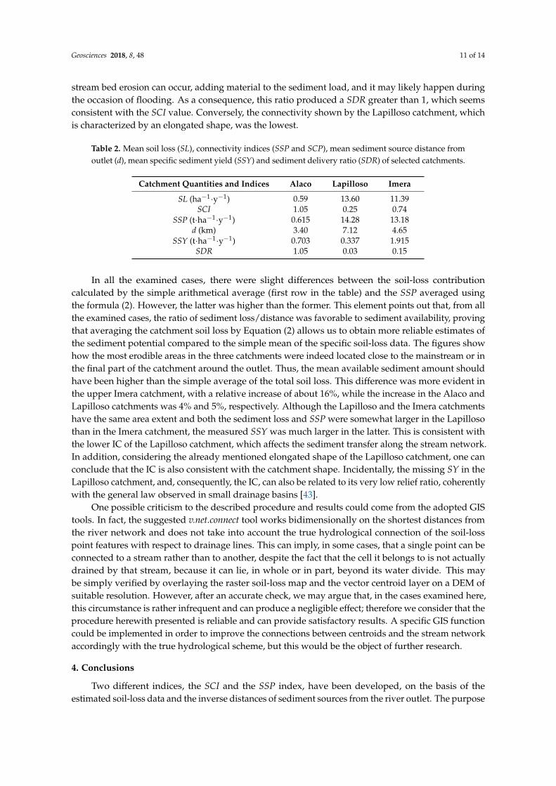
stream bed erosion can occur, adding material to the sediment load, and it may likely happen duringthe occasion of flooding. As a consequence, this ratio produced a SDR greater than 1, which seemsconsistent with the SCI value. Conversely, the connectivity shown by the Lapilloso catchment, whichis characterized by an elongated shape, was the lowest.

Table 2. Mean soil loss (SL), connectivity indices (SSP and SCP), mean sediment source distance fromoutlet (d), mean specific sediment yield (SSY) and sediment delivery ratio (SDR) of selected catchments.

Catchment Quantities and Indices Alaco Lapilloso Imera

SL (ha−1·y−1) 0.59 13.60 11.39SCI 1.05 0.25 0.74

SSP (t·ha−1·y−1) 0.615 14.28 13.18d (km) 3.40 7.12 4.65

SSY (t·ha−1·y−1) 0.703 0.337 1.915SDR 1.05 0.03 0.15

In all the examined cases, there were slight differences between the soil-loss contributioncalculated by the simple arithmetical average (first row in the table) and the SSP averaged usingthe formula (2). However, the latter was higher than the former. This element points out that, from allthe examined cases, the ratio of sediment loss/distance was favorable to sediment availability, provingthat averaging the catchment soil loss by Equation (2) allows us to obtain more reliable estimates ofthe sediment potential compared to the simple mean of the specific soil-loss data. The figures showhow the most erodible areas in the three catchments were indeed located close to the mainstream or inthe final part of the catchment around the outlet. Thus, the mean available sediment amount shouldhave been higher than the simple average of the total soil loss. This difference was more evident inthe upper Imera catchment, with a relative increase of about 16%, while the increase in the Alaco andLapilloso catchments was 4% and 5%, respectively. Although the Lapilloso and the Imera catchmentshave the same area extent and both the sediment loss and SSP were somewhat larger in the Lapillosothan in the Imera catchment, the measured SSY was much larger in the latter. This is consistent withthe lower IC of the Lapilloso catchment, which affects the sediment transfer along the stream network.In addition, considering the already mentioned elongated shape of the Lapilloso catchment, one canconclude that the IC is also consistent with the catchment shape. Incidentally, the missing SY in theLapilloso catchment, and, consequently, the IC, can also be related to its very low relief ratio, coherentlywith the general law observed in small drainage basins [43].

One possible criticism to the described procedure and results could come from the adopted GIStools. In fact, the suggested v.net.connect tool works bidimensionally on the shortest distances fromthe river network and does not take into account the true hydrological connection of the soil-losspoint features with respect to drainage lines. This can imply, in some cases, that a single point can beconnected to a stream rather than to another, despite the fact that the cell it belongs to is not actuallydrained by that stream, because it can lie, in whole or in part, beyond its water divide. This maybe simply verified by overlaying the raster soil-loss map and the vector centroid layer on a DEM ofsuitable resolution. However, after an accurate check, we may argue that, in the cases examined here,this circumstance is rather infrequent and can produce a negligible effect; therefore we consider that theprocedure herewith presented is reliable and can provide satisfactory results. A specific GIS functioncould be implemented in order to improve the connections between centroids and the stream networkaccordingly with the true hydrological scheme, but this would be the object of further research.

4. Conclusions

Two different indices, the SCI and the SSP index, have been developed, on the basis of theestimated soil-loss data and the inverse distances of sediment sources from the river outlet. The purpose

Geosciences 2018, 8, 48 12 of 14

was to express, in simplified form, two basic characteristics of a catchment, that is, the sediment transfercapacity and the potentially available sediment amount via the river network.

Although the proposed indices are both related to the distance from the outlet, the first is inthe form of an adimensional index, while the second represents the weighted mean of the soil loss(t·ha−1·y−1) at the catchment scale.

Despite possible shortcomings linked to the functionality of the suggested GIS tools, which areproved to be of marginal significance, the ease of the GIS approach and the use of available databasesand tools make the methodology usable and repeatable.

The discussed results have pointed out the complementarity between the proposed indices,which may be used together or alternatively as a proxy for the sediment potential of a catchment.More specifically, in combination with geomorphometric and hydrological parameters, in order tocomprise the whole range of variables affecting the SY, these indices can help in refining theoreticalmodels for the assessment of the SY in ungauged river basins.

Acknowledgments: The authors thank the European Soil Data Centre (ESDAC) (https://esdac.jrc.ec.europa.eu/),European Commission, Joint Research Centre, for making available the soil-loss data. The authors also thank theanonymous reviewers for their valuable comments and suggestions.

Author Contributions: Sergio Grauso is the main author who initiated the idea and wrote the manuscript;Francesco Pasanisi and Carlo Tebano performed the GIS elaborations and model implementation and contributedto the final writing of the manuscript.

Conflicts of Interest: The authors declare no conflict of interest.

References

1. Wischmeier, W.H.; Smith, D.D. Predicting rainfall erosion losses—A guide to conservation planning.In US Department of Agriculture, Agriculture Handbook No. 537; US Government Printing Office: Washington,DC, USA, 1978.

2. Renard, K.G.; Foster, G.R.; Weesies, G.A.; Porter, J.P. RUSLE—Revised universal soil loss equation. J. SoilWater Conserv. 1991, 46, 30–33.

3. Renard, K.G.; Foster, G.R.; Weesies, G.A.; McCool, D.K.; Yoder, D.C. Predicting soil erosion by water—Aguide to conservation planning with the revised universal soil loss equation (RUSLE). In US Department ofAgriculture, Agriculture Handbook No. 703; US Government Printing Office: Washington, DC, USA, 1997.

4. Wolman, M.G. Changing needs and opportunities in the sediment field. Water Resour. Res. 1977, 13, 50–54.[CrossRef]

5. Walling, D.E. The sediment delivery problem. J. Hydrol. 1983, 65, 209–237. [CrossRef]6. Ferro, V.; Minacapilli, M. Sediment delivery processes at basin scale. Hydrol. Sci. J. 1995, 40, 703–717.

[CrossRef]7. Dedkov, A. The relationship between sediment yield and drainage basin area. In Sediment Transfer through

the Fluvial System, Proceedings of the International Symposium Held in Moscow, Russia, 2–6 August 2004;IAHS Publications: Wallingford, UK, 2004.

8. Lu, H.; Moran, C.; Prosser, I.; Sivapalan, M. Modelling sediment delivery ratio based on physical principles.In Proceedings of the 2nd International Congress on Environmental Modelling and Software, Osnabrück,Germany, 14–17 June 2004.

9. Lenhart, T.; Van Rompaey, A.; Steegen, A.; Fohrer, N.; Frede, H.-G.; Govers, G. Considering spatialdistribution and deposition of sediment in lumped and semi-distributed models. Hydrol. Process. 2005, 19,785–794. [CrossRef]

10. Diodato, N.; Grauso, S. An improved correlation model for sediment delivery ratio assessment.Environ. Earth Sci. 2009, 59, 223–231. [CrossRef]

11. Vigiak, O.; Borselli, L.; Newham, L.T.H.; McInnes, J.; Roberts, A.M. Comparison of conceptual landscapemetrics to define hillslope-scale sediment delivery ratio. Geomorphology 2012, 138, 74–88. [CrossRef]

12. Hooke, J. Coarse sediment connectivity in river channel systems: A conceptual framework and methodology.Geomorphology 2003, 56, 79–94. [CrossRef]

Geosciences 2018, 8, 48 13 of 14

13. Pilotti, M.; Bacchi, B. Distributed evaluation of the contribution of soil erosion to the sediment yield froma watershed. Earth Surface Process. Landf. 1997, 22, 1239–1251. [CrossRef]

14. Cammeraat, L.H. A review of two strongly contrasting geomorphological systems within the context ofscale. Earth Surface Process. Landf. 2002, 27, 1201–1222. [CrossRef]

15. Masselink, R.J.H.; Heckmann, T.; Temme, A.J.A.M.; Anders, N.S.; Gooren, H.P.A.; Keesstra, S.D. A networktheory approach for a better understanding of overland flow connectivity. Hydrol. Process. 2017, 31, 207–220.[CrossRef]

16. Fryirs, K.A.; Brierley, G.J.; Preston, N.J.; Spencer, J. Catchment-scale (dis)connectivity in sediment flux in theupper Hunter catchment, New South Wales, Australia. Geomorphology 2007, 84, 297–316. [CrossRef]

17. Gumiere, S.J.; Le Bissonnais, Y.; Raclot, D.; Cheviron, B. Vegetated filter effects on sedimentologicalconnectivity of agricultural catchments in erosion modelling: A review. Earth Surface Process. Landf. 2011, 36,3–19. [CrossRef]

18. López-Vicente, M.; Nadal-Romero, E.; Cammeraat, L.H. Hydrological connectivity does change over 70 yearsof abandonment and afforestation in the Spanish Pyrenees. Land Degrad. Dev. 2016, 28, 1298–1310. [CrossRef]

19. Borselli, L.; Cassi, P.; Torri, D. Prolegomena to sediment and flow connectivity in the landscape: A GIS andfield numerical assessment. Catena 2008, 75, 268–277. [CrossRef]

20. Cavalli, M.; Trevisani, S.; Comiti, F.; Marchi, L. Geomorphometric assessment of spatial sediment connectivityin small Alpine catchments. Geomorphology 2013, 188, 31–41. [CrossRef]

21. Brardinoni, F.; Cavalli, M.; Heckmann, T.; Liébault, F.; Rimböck, A. Guidelines for Assessing SedimentDynamics in Alpine Basins and Channel Reaches. Available online: http://www.sedalp.eu/download/dwd/reports/WP4_Report.pdf (accessed on 6 November 2017).

22. López-Vicente, M.; Álvarez, S. Influence of DEM resolution on modelling hydrological connectivity ina complex agricultural catchment with woody crops. Earth Surface Process. Landf. 2017. [CrossRef]

23. Cantreul, V.; Bielders, C.; Calsamiglia, A.; Degré, A. How pixel size affects a sediment connectivity index incentral Belgium. Earth Surface Process. Landf. 2017. [CrossRef]

24. López-Vicente, M.; Poesen, J.; Navas, A.; Gaspar, L. Predicting runoff and sediment connectivity and soilerosion by water for different land use scenarios in the Spanish Pre-Pyrenees. Catena 2013, 102, 62–73.[CrossRef]

25. López-Vicente, M.; Quijano, L.; Palazón, L.; Gaspar, L. Assessment of soil redistribution at catchmentscale by coupling a soil erosion model and a sediment connectivity index (Central Spanish Pre-Pyrenees).Cuad. Investig. Geogr. 2015, 141, 127–147. [CrossRef]

26. Cammeraat, L.H.; van Beek, L.P.H.; Dooms, T. Modelling Water and Sediment Connectivity Patternsin a Semi-Arid Landscape. Available online: https://pure.uva.nl/ws/files/1083710/71066_murcia.pdf(accessed on 6 November 2017).

27. Sklar, L.S.; Riebe, C.S.; Lukens, C.E.; Bellugi, D. Catchment power and the joint distribution of elevation andtravel distance to the outlet. Earth Surface Dyn. 2016, 4, 799–818. [CrossRef]

28. Heckmann, T.; Schwanghart, W. Geomorphic coupling and sediment connectivity in an alpinecatchment—Exploring sediment cascades using graph theory. Geomorphology 2013, 182, 89–103. [CrossRef]

29. Cossart, É.; Fressard, M. Assessment of structural sediment connectivity within catchments: Insights fromgraph theory. Earth Surface Dyn. 2017, 5, 253–268. [CrossRef]

30. Heckmann, T.; Vericat, D. Inferring sediment connectivity from high-resolution DEMs of Difference.In Proceedings of the European Geosciences Union General Assembly 2017, Vienna, Austria, 23–28 April 2017.

31. SedAlp Project. Sediment Management in Alpine Basins. Available online: http://www.sedalp.eu/project/(accessed on 6 November 2017).

32. Connecteur Project. Connecting European Connectivity Research (COST Action No. ES1306). Available online:http://connecteur.info/ (accessed on 6 November 2017).

33. Crema, S.; Cavalli, M. SedInConnect: A stand-alone, free and open source tool for the assessment of sedimentconnectivity. Comput. Geosci. 2018, 111, 39–45. [CrossRef]

34. Panagos, P.; Borrelli, P.; Poesen, J.; Ballabio, C.; Lugato, E.; Meusburger, K.; Montanarella, L.; Alewell, C.The new assessment of soil loss by water erosion in Europe. Environ. Sci. Policy 2015, 54, 438–447. [CrossRef]

35. Lane, L.J.; Hernandez, M.; Nichols, M. Processes controlling sediment yield from watersheds as functions ofspatial scale. Environ. Model. Softw. 1997, 12, 355–369. [CrossRef]

Geosciences 2018, 8, 48 14 of 14

36. Verstraeten, G.; Poesen, J. Factors controlling sediment yield from small intensively cultivated catchments ina temperate humid climate. Geomorphology 2001, 40, 123–144. [CrossRef]

37. Verstraeten, G.; Poesen, J.; de Vente, J.; Koninckx, X. Sediment yield variability in Spain: A quantitative andsemiqualitative analysis using reservoir sedimentation rates. Geomorphology 2003, 50, 327–348. [CrossRef]

38. De Vente, J.; Poesen, J. Predicting soil erosion and sediment yield at the basin scale: Scale issues andsemi-quantitative models. Earth-Sci. Rev. 2005, 71, 95–125. [CrossRef]

39. QGIS. A Free and Open Source Geographic Information System. Available online: http://www.qgis.org/(accessed on 6 November 2017).

40. Neteler, M.; Bowman, M.H.; Landa, M.; Metz, M. GRASS GIS: A multi-purpose open source GIS.Environ. Model. Softw. 2012, 31, 124–130. [CrossRef]

41. Tebano, C.; Pasanisi, F.; Grauso, S. QMorphoStream: Processing tools in QGIS environment for thequantitative geomorphic analysis of watersheds and river networks. Earth Sci. Inf. 2017, 10, 257–268.[CrossRef]

42. National Geoportal. Access Point to Environmental and Territorial Information. Available online:http://www.pcn.minambiente.it/mattm/en/ (accessed on 6 November 2017).

43. Hadley, R.; Schumm, S. Sediment sources and drainage basin characteristics in upper cheyenneriver basin. In US Geological Survey, Water Supply Paper No. 1531-B; US Government Printing Office:Washington, DC, USA, 1961.

© 2018 by the authors. Licensee MDPI, Basel, Switzerland. This article is an open accessarticle distributed under the terms and conditions of the Creative Commons Attribution(CC BY) license (http://creativecommons.org/licenses/by/4.0/).