Western University Western University

Scholarship@Western Scholarship@Western

Electronic Thesis and Dissertation Repository

9-29-2017 3:00 PM

Assessment of Earthquake Site Amplification and Application of Assessment of Earthquake Site Amplification and Application of

Passive Seismic Methods for Improved Site Classification in the Passive Seismic Methods for Improved Site Classification in the

Greater Vancouver Region, British Columbia Greater Vancouver Region, British Columbia

Frederick Andrew Jackson, The University of Western Ontario

Supervisor: Dr. Sheri Molnar, The University of Western Ontario

A thesis submitted in partial fulfillment of the requirements for the Master of Science degree in

Geophysics

© Frederick Andrew Jackson 2017

Follow this and additional works at: https://ir.lib.uwo.ca/etd

Part of the Geophysics and Seismology Commons

Recommended Citation Recommended Citation Jackson, Frederick Andrew, "Assessment of Earthquake Site Amplification and Application of Passive Seismic Methods for Improved Site Classification in the Greater Vancouver Region, British Columbia" (2017). Electronic Thesis and Dissertation Repository. 4938. https://ir.lib.uwo.ca/etd/4938

This Dissertation/Thesis is brought to you for free and open access by Scholarship@Western. It has been accepted for inclusion in Electronic Thesis and Dissertation Repository by an authorized administrator of Scholarship@Western. For more information, please contact wlswadmin@uwo.ca.

i

Abstract

There is renewed interest to improve seismic microzonation mapping in Greater Vancouver,

British Columbia (BC). We investigate local geology as the cause of observed variable

ground shaking from the 2015 M 4.7 Vancouver Island earthquake. We observe high

amplification at 4-6 Hz on thick sediment and the northern edge of the Fraser River delta,

and disparities with current regional seismic microzonation mapping. Site amplification and

shear-wave velocity (VS) are assessed from the first borehole earthquake recordings in BC.

We also perform ambient vibration analyses at 13 new locations in southwest BC to highlight

suitability of passive seismic methods for improving regional microzonation. We obtain well-

resolved VS profiles from joint inversion of dispersion curves and horizontal to vertical

spectral ratios. The corresponding National Building Code of Canada site classifications vary

between D and C. This study is a notable contribution to public earthquake site assessments

in the Greater Vancouver region.

Keywords

Earthquakes, ground motion, site effects, site classification, site response, shear wave

velocity, microtremors, ambient vibrations, microzonation, surface wave dispersion

ii

Co-authorship statement

The thesis is prepared in Integrated Article format and consists of the following two papers

that are either published or submitted to peer-reviewed journals.

Chapter 2: Jackson, F., Molnar, S., Ghofrani, H., Atkinson, G.M., Cassidy, J.F.,

Assatourians, K. Ground Motions of the December 2015 M 4.7 Vancouver Island

Earthquake: Attenuation and Site Response. Bulletin of the Seismological Society of America,

accepted.

Strong-motion recordings were obtained by my supervisor. I generated my own Python codes

(ObsPy) to perform all processing of strong-motion earthquake recordings (e.g., filtering,

Fourier transformation, spectral ratios) and their interpretation with regards to previous

studies and microzonation mapping. My work was combined with attenuation analyses of

broad-band seismograph recordings accomplished by Dr. Hadi Ghofrani to comprise the full

article and reviewed by our co-authors. Only my strong-motion analyses (second half of

article) appear here in this thesis.

Chapter 3: Jackson, F., Molnar, S., Ventura, CE. Application of passive seismic methods at

13 school sites to improve earthquake site assessment in the Greater Vancouver region,

British Columbia, Canada. This paper will be submitted to the Canadian Geotechnical

Journal or the Canadian Journal of Civil Engineering.

Passive seismic recordings were collected and provided by my supervisor. I performed all the

ambient vibration analyses and inversions for each site using Geopsy software. I generated a

Matlab script to efficiently display Geopsy results and produce figures for publication. I

obtained previous studies with independent datasets to compare and interpret my results.

The thesis and integrated articles were completed under the supervision of Dr. Sheri Molnar.

Dr. Molnar provided on-going guidance, suggestions, and improvements to the manuscripts

and assisted with manuscript revisions.

iii

Acknowledgments

Financial support for this thesis was provided by an NSERC Collaborative Research and

Development (CRD) grant with Chaucer Syndicates and the Institute for Catastrophic Loss

Reduction.

I’m enormously grateful to my supervisor Sheri. She provided me with the opportunity to

study my MSc at Western, and throughout my years of study has been incredibly supportive

and open to any questions I had.

I’d also like to thank all the coauthors of my BSSA paper: Hadi Ghofrani, Gail M. Atkinson,

Karen Assatourians, and John Cassidy. Their kind guidance during my project and their

contributions to the published paper are much appreciated.

Finally, I must express my profound thanks to my friends and family for all their support.

This accomplishment would not have been possible without them.

iv

Table of Contents

Abstract ................................................................................................................................ i

Keywords ............................................................................................................................. i

Co-authorship statement ..................................................................................................... ii

Acknowledgments.............................................................................................................. iii

Table of Contents ............................................................................................................... iv

List of Tables .................................................................................................................... vii

List of Figures .................................................................................................................. viii

List of Appendices ...............................................................................................................x

List of Abbreviations ......................................................................................................... xi

List of Symbols ................................................................................................................. xii

Chapter 1 ............................................................................................................................1

1. Introduction ...................................................................................................................1

Seismic risk in British Columbia ................................................................................1

Project Aims ...............................................................................................................3

Seismological theory ..................................................................................................3

Site Effects .................................................................................................................4

Earthquake Site Classification ....................................................................................6

1.5.1. Proxy methods for VS30 .................................................................................... 7

1.5.2. Alternatives to VS30 .......................................................................................... 8

Organization of work ..................................................................................................9

1.6.1. Chapter 2 .......................................................................................................... 9

1.6.2. Chapter 3 ........................................................................................................ 10

1.6.3. Chapter 4 ........................................................................................................ 10

References ................................................................................................................10

Chapter 2 ..........................................................................................................................14

2. Observed site response of the 30 December 2015 M 4.7 Vancouver Island earthquake

………................................................................................................................................14

Introduction ..............................................................................................................14

2.1.1. Aims and Objectives ...................................................................................... 15

Local geology and site amplification .......................................................................15

2.2.1. Greater Vancouver ......................................................................................... 15

v

2.2.2. Greater Victoria ............................................................................................. 17

Strong Motion Analysis ............................................................................................17

2.3.1. Dataset............................................................................................................ 17

2.3.2. Spatial variation of ground motions ............................................................... 18

2.3.3. Borehole array recordings .............................................................................. 25

2.3.4. Site amplification with depth ......................................................................... 26

2.3.5. Downhole cross correlation analysis ............................................................. 29

Conclusions ..............................................................................................................30

Data and Resources ..................................................................................................31

Acknowledgements ..................................................................................................31

References ................................................................................................................32

Chapter 3 ..........................................................................................................................35

3. Application of passive seismic methods at 13 school sites to improve earthquake site

assessment in the Greater Vancouver region .....................................................................35

Introduction ..............................................................................................................35

3.1.1. Earthquake site classification ......................................................................... 35

3.1.2. Proxy methods for VS30 .................................................................................. 37

3.1.3. Aims and objectives ....................................................................................... 37

Geological Setting and Previous Site Classifications ...............................................39

Theoretical Background ...........................................................................................42

3.3.1. Single station HVSR ...................................................................................... 42

3.3.2. Surface wave array methods .......................................................................... 43

Passive Seismic Recordings .....................................................................................46

3.4.1. Data collection ............................................................................................... 46

3.4.2. MHVSR analysis ........................................................................................... 47

3.4.3. Dispersion analysis ........................................................................................ 49

Inversion ...................................................................................................................52

3.5.1. The neighbourhood algorithm ........................................................................ 53

3.5.2. Joint inversion implementation ...................................................................... 54

Retrieved VS Profiles ................................................................................................56

3.6.1. VS profile interpretation ................................................................................. 60

3.6.2. Site classification comparison........................................................................ 62

Discussion and Conclusions .....................................................................................64

Acknowledgements ..................................................................................................65

vi

References ................................................................................................................65

Chapter 4 ..........................................................................................................................72

4. Conclusions .................................................................................................................72

Summary ..................................................................................................................72

Discussion ................................................................................................................73

Future Work .............................................................................................................75

References ................................................................................................................76

Appendices .........................................................................................................................78

Curriculum Vitae ...............................................................................................................80

vii

List of Tables

Table 1.1. A summary of the seismic site categories in the 2010 NBCC (NRC, 2010) ........... 7

Table 2.1. Stratigraphic summary of the borehole arrays. ...................................................... 25

Table 3.1. Details of array geometry. ..................................................................................... 47

Table 3.2. Site classification estimates from our joint inversion results compared to previous

classification estimates for our 13 sites (sorted by site class). .......................................... 63

viii

List of Figures

Figure 1.1. Tectonic setting of the northern Cascadia Subduction Zone. Arrows show relative

plate motions. (Modified from Earle, 2016). ...................................................................... 2

Figure 2.1. Variation in peak ground acceleration at strong motion stations across southwest

BC are shown by filled circles. The M 4.7 earthquake focal mechanism (beach ball)

denotes the earthquake epicentre and locations of three borehole arrays (B1-B3) are

shown by triangles. ........................................................................................................... 19

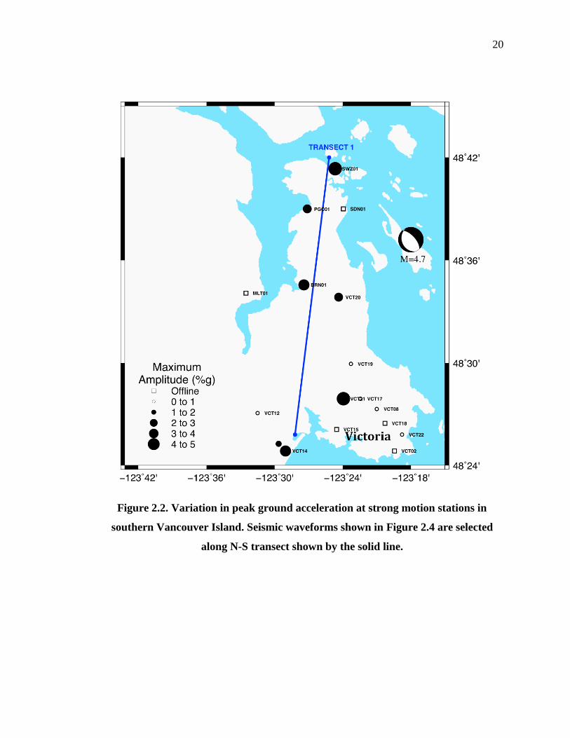
Figure 2.2. Variation in peak ground acceleration at strong motion stations in southern

Vancouver Island. Seismic waveforms shown in Figure 2.4 are selected along N-S

transect shown by the solid line. ....................................................................................... 20

Figure 2.3. Variation in peak ground acceleration at strong motion stations in southwest

Greater Vancouver. Seismic waveforms shown in Figure 2.4 are selected along two NE-

SW transects shown by the solid lines. Background shading corresponds to amplification

hazard rating, modified from Monahan (2005). ................................................................ 21

Figure 2.4. Transverse component seismic waveforms along transects labelled in Figure 2.2

and Figure 2.3. Y-axis is acceleration in units of g, plotted to ± 0.05 g. Background

shading corresponds to amplification hazard site class assigned by S. Molnar for Victoria

stations and Monahan (2005) for Vancouver stations as in Figure 2.2. ........................... 22

Figure 2.5. (a) Transverse-component Fourier acceleration spectra at select IA stations across

the Fraser delta, compared to a station on Pleistocene till in downtown Vancouver

(VNC13). (b) Cartoon cross-section of the Fraser River delta with select strong-motion

stations labelled and shown by black squares (modified from Cassidy and Rogers, 1999).

........................................................................................................................................... 24

Figure 2.6. Earthquake HVSRs obtained at particular depths within the three borehole arrays.

........................................................................................................................................... 27

Figure 2.7. Upper-to-lower spectral ratios (depths are reported in each legend) determined

within each borehole array. ............................................................................................... 28

ix

Figure 2.8. Interval VS determined within each borehole arrays. Black dots correspond to

sensor depth. ..................................................................................................................... 30

Figure 3.1. Locations of 13 school sites (filled circles) in southwest BC. Major urban centres

are labelled and marked by small black circles. ............................................................... 38

Figure 3.2. School site locations in Greater Vancouver denoted by filled circles. Locations of

relevant stratigraphic profiles are shown by numbered squares, which are detailed in

Armstrong (1984). Background map shading exhibits simplified geology (Turner et al.,

1997); lowland (Holocene) sediment shown in beige, uplands (Pleistocene) sediment

shown in blue, and Tertiary bedrock shown in pink. ........................................................ 40

Figure 3.3. Site classification maps from (a) VS data (modified from Hunter and Christian,

2001), (b) sparse VS data combined with Quaternary mapping (modified from Monahan,

2005), and (c) proxy-VS30 estimates based on topographic slope (Allen and Wald, 2009).

........................................................................................................................................... 41

Figure 3.4. (a) Overview map of 8-sensor acquisition arrays at Burnaby (modified from

Google Maps, 2017). Each circle denotes the location of a Tromino® microtremor

recording, coloured by each array radius, ranging from 5 to 25 m. (b) Photo of 5-m array

at Burnaby (Photo credit Sheri Molnar)............................................................................ 46

Figure 3.5. Time-averaged MHVSR curves representative for each site are shown with one

standard deviation. ............................................................................................................ 48

Figure 3.6. Final MSPAC dispersion curves picked for 11 sites shown by black squares.

MSPAC histogram for all arrays at each site shown in blue, where darker shading

indicates higher histogram count. ..................................................................................... 51

Figure 3.7. Panels from left to right for each site are average (black solid line) and one

standard deviation (black dashed line) MHVSR and dispersion (squares) datasets, and

inversion results shown as VS depth profiles (blue lines). Synthetic MHVSR and

dispersion curves of the inverted models are shown in panels to the left with similar

model shading. .................................................................................................................. 57

x

List of Appendices

Figure A1. Time-averaged MHVSR for Tsawwassen shown with one standard

deviation…………………………………………………………………………….……78

Figure A2. MSPAC histogram stacked cumulatively for East Vancouver arrays shown in

blue, where darker shading indicates higher histogram

count.………………………….…………………………………………………...…78

Figure A3. MSPAC histogram stacked cumulatively for Killarney arrays shown in blue,

where darker shading indicates higher histogram

count………………………………………………………………………………….79

xi

List of Abbreviations

1D One-dimensional

2D Two-dimensional

3D Three-dimensional

BC British Columbia

BC MoTI BC Ministry of Transportation and Infrastructure

BCSIMS BC Smart Infrastructure Monitoring System

CHBDC Canadian Highway and Bridge Design Code

CSZ Cascadia Subduction Zone

EHVSR Earthquake Horizontal-to-Vertical spectral ratio

FK Frequency Wavenumber

GMPE Ground Motion prediction Equation

HRFK High Resolution Frequency Wavenumber method

HVSR Horizontal-to-Vertical spectral ratio

IA Internet accelerometer

MASW Multichannel Analysis of Surface Waves

MHVSR Microtremor Horizontal-to-Vertical spectral ratio

MSPAC Modified Spatial Auto Correlation

NBCC National Building Code of Canada

NEHRP National Earthquake Hazards Reduction Program

NRC Natural Resources Canada

PGA Peak ground acceleration (%g)

SASW Spectral Analysis of Surface Waves

SH Transversely-polarised shear wave

SV Vertically-polarised shear wave

SPAC Spatial Auto Correlation method

xii

List of Symbols

A Impedance amplification

f0 Fundamental peak frequency (Hz)

g Acceleration due to gravity (m/s2)

fpeak Response peak frequency (Hz)

h Layer thickness (m)

kmax Aliasing Limit

kmin Resolution Limit

M Moment Magnitude

n Normal mode number

Rhypo Hypocentral distance (km)

VS Shear-wave velocity (m/s)

VS30 Time-averaged shear-wave velocity of the upper 30 meters (m/s)

VSave Time-averaged shear-wave velocity of the soil layer (m/s)

ρ Density (kg/m3)

1

Chapter 1

1. Introduction

Seismic risk in British Columbia

Greater Vancouver is the largest metropolitan area in British Columbia (BC), and is the

highest earthquake risk city in Canada due to significant exposure to high hazard. As the

third largest city in Canada, it encompasses a population of 2.5 million, as well as key

infrastructure including Canada’s second busiest airport, the fourth largest tonnage port in

North America, and 22 major bridge and tunnel crossings. Greater Victoria, the

provincial capital, is located at the southern tip of Vancouver Island and includes a

population of 345,000; the island relies on submarine electrical transmission cables, and

ferry terminals for 95% of its food supply, from the BC mainland. A report

commissioned by the Insurance Bureau of Canada (AIR Worldwide, 2013) estimates that

a moment magnitude (M) 9.0 earthquake in BC would cause $62 billion in direct

damages, and an additional $12.7 billion in indirect impact (e.g. supply chain

interruption, infrastructure damage).

60% of Canada’s earthquakes occur along BC’s coast (Natural Resources Canada, 2016).

The high seismic hazard in this region arises from the 1000 km long Cascadia Subduction

Zone (CSZ), which stretches from Vancouver Island to northern California and marks the

subduction of the Juan de Fuca plate under the North American plate (Figure 1.1). This

zone is bounded by two transform faults: the Queen Charlotte Fault to the north, and the

San Andreas Fault to the south. Southwest BC is located at the northern end of the CSZ

(see Figure 1.1). Southwest BC is a region of complex deformation above a bend in the

subducting plate. Crustal structure here in the continental margin is composed of accreted

metamorphic and igneous terranes with various mapped faults at surface and at depth

(Balfour, 2011). As is common with subduction zones, the CSZ is associated with a chain

of andesitic volcanoes that extend from northern California to southern BC (Clague,

1997).

2

Figure 1.1. Tectonic setting of the northern Cascadia Subduction Zone. Arrows

show relative plate motions. (Modified from Earle, 2016).

Southwest BC is one of the most seismically active regions in Canada: more than 100

offshore earthquakes of magnitude 5 or greater have occurred in the last 70 years

(CREW, 2011). The complex tectonic setting gives rise to three types of earthquakes:

those originating at the subduction interface (interplate), inside the subducting plate

(inslab/intraplate), and at shallow faults in the crust (crustal). The largest instrumentally

recorded earthquake in Canada was the 1949 M 8.1 crustal event near Haida Gwaii

(Natural Resources Canada, 2016), which originated from the strike-slip movement of the

Queen Charlotte Fault. The magnitude of inslab events is usually lower than M 7, but due

to their high rate of occurrence, make the largest contribution to seismic hazard in the

region (Bent & Greene, 2012), particularly short-period ground shaking. Most recently,

motions of the 2015 M 4.7 Vancouver Island inslab earthquake demonstrated high stress

(Brune source model) but lower shaking levels than expected (GMPEs are not well tuned

to this low magnitude level; Jackson et al., 2017). In addition, there is significant

3

evidence that the Juan de Fuca and North America plates are currently locked together

(Clague, 1997), allowing the possibility of a sudden release of the accumulating strain

resulting in a rare subduction “megathrust” earthquake, like the 1700 Cascadia

megathrust earthquake, estimated as M 8.7-9.2 (Satake et al., 2003). However these

mega-thrust events occur on average only once every 500 years.

Because of the significant seismic hazard in southwest BC, it is vital to predict future

earthquake ground motions as accurately as possible. The accuracy of seismic hazard

estimates affects building codes and earthquake risk and loss estimations. Effective risk

assessment affects the government’s ability to save lives and money by identifying at risk

regions and structures and to guide decisions on resource allocation.

Project Aims

In response to renewed interest to improve seismic microzonation mapping in Greater

Vancouver, we aim to first qualify the accuracy of current microzonation mapping in the

region, and secondly test the suitability of non-invasive seismic techniques to address

these issues by site-specific VS profiling. Specifically we aim to determine important

parameters that govern site response, e.g., VS profile(s), fundamental peak frequencies,

and depths of significant impedance contrasts.

The overall impact of this study is to add to the database of knowledge on seismic

velocities in Metropolitan Vancouver as a continuation of passive-seismic site

characterization case studies in BC (Molnar et al., 2010; Molnar et al., 2013; Molnar et

al., 2014) which serve as the basis for a 5-year seismic microzonation effort in the region.

Accurate VS mapping will improve the hazard mapping in the region and thus the ground

motion prediction and risk estimation.

Seismological theory

Energy released by an earthquake propagates as two basic types: body waves which

travel directly from the earthquake focus through the Earth’s interior, and surface waves

generated by the interaction of body waves at the Earth’s surface, which travel laterally

4

along the free boundary of the surface. Body waves consist of compressional or primary

(P) waves, which propagate longitudinally along the direction of motion, and shear or

secondary (S) waves, which propagate radially to the direction of motion. Shear waves

can also be polarised into either perpendicular plane by geological interaction into either

SH (shear-horizontal) or SV (shear-vertical). P-waves travel fastest with low amplitude,

and S-waves travel slower with higher amplitude due to the conservation of energy.

Surface waves consist of two types: Love waves consisting of a horizontally polarised

(SH) S-wave trapped in the upper layers of the surface, and Rayleigh waves generated by

the interference between a lateral P-wave and an SV-wave. Surface waves travel slower

than body waves and arrive last, but with considerably higher amplitude and duration,

meaning that they commonly cause the most destruction in an earthquake event.

Commonly the horizontal shear motions are the most significant component of seismic

load in ordinary buildings (Panza et al. 2004), and therefore the most damaging aspect of

earthquake shaking. Because of this, high amplitude Love waves tend to be the most

damaging wave, as well as standard S-waves propagating close to the earthquake source

where their amplitudes have not yet decayed by geometric attenuation. For moderate

earthquakes, the peak ground acceleration (PGA) is the main control of observed damage,

however in severe earthquakes damage is mainly controlled by the peak ground velocity

(Worden & Wald, 2016).

Site Effects

In many historical and recent earthquakes local geology and soil conditions have notably

altered the amplitude, frequency content and duration of ground motion, resulting in

significant variation across small regions. A notable case study for the contribution of site

effects is the 1985 M 8.0 Mexico City earthquake, where the city experienced

catastrophic damage on soft lake bed deposits from the megathrust event over 350 km

away (Seed et al., 1988). This phenomenon is known as site effects, and includes

amplification and resonance from the one-dimensional (1D) soil column as well as from

two- (2D) and three-dimensional (3D) basins and topography. Observed amplification is

5

also affected by complex dynamic properties of soil (damping, plasticity, liquefaction)

however these effects are not further considered in this thesis. Site effects can often be

adequately described by 1D models, although in areas of strong lateral variations a spatial

understanding of site effects is required (Sánchez-Sesma, 1987). Proper characterization

of site conditions is a major component of seismic hazard analysis and required for

accurate ground motion prediction.

There are two major site effect factors that amplify ground motion as seismic waves

propagate through a 1D column of soil (profile): shear wave velocity (VS), and

impedance contrast thickness. Firstly, VS of a material is directly related to the stiffness,

and seismic waves travel slower and with higher amplitude through soft sediments

compared to stiff material due to the conservation of energy. As previously stated, the

horizontal shear motions are commonly the most significant component of seismic load

in ordinary buildings (Panza et al. 2004), i.e. the SH component in both S-wave and Love

wave propagation. Therefore VS is a major control of earthquake damage.

Because shear waves refract towards the vertical as they propagate through less stiff

layers towards surface, and because the direction of particle motion is perpendicular to

propagation, amplification is observed in the horizontal component of motion. For a

single soil layer (subscript 1) over an elastic half-space (subscript 2), the theoretical 1D

impedance amplification (A) is:

𝐴 = √

𝜌2𝑉𝑆2

𝜌1𝑉𝑆1, (1.1)

where ρ is density.

Secondly, when a site consists of soft surficial material, its thickness and the depth to a

major impedance contrast such as stiff bedrock has a large effect on amplification. The

resonance amplification is equal to Equation 1.1 squared, which occurs at the following

frequencies:

𝑓 = (2𝑛 + 1) (𝑉𝑆𝑎𝑣𝑒

4ℎ), (1.2)

6

where n is the normal mode number (defined by the number of half-sinusoidal waves in

the vibration), VSave is the average velocity of the soil layer, and h is thickness. The

described 1D site amplification defines a SH-wave transfer function or amplification

frequency spectrum. Soils behave nonlinearly when earthquake shaking is strong, i.e.,

~10 %g, where g is the acceleration due to gravity. 1D earthquake site response includes

the nonlinear behaviour of the soil itself when shaken by dynamic earthquake shaking.

Prediction or modelling of 1D earthquake site response includes VS and ρ (small-strain

shear modulus; Gmax = ρVS2) as well as shear modulus reduction and damping curves

established for various soil types (e.g., Seed & Idriss, 1970).

Site characterization includes field and laboratory methods to measure properties (i.e., VS

and ρ) of the subsurface geologic material at the site to describe and ultimately predict

earthquake site effects. Field techniques can be geotechnical (standard penetration tests,

pressure meter tests, seismic cone penetration tests, etc.) or geophysical (active- or

passive-source surface wave methods). Geophysical (seismic) field techniques are much

faster and non invasive, and are better suited for a large-scale site characterization

project. Mapping large-scale seismic hazard variation due to site conditions is known as

seismic microzonation mapping, and typically includes amplification, liquefaction, and

landslide and rock fall hazard mapping. Such microzonation maps help make informed

decisions for urban planning, and mitigation and adaption for an urban centre or a region.

Earthquake Site Classification

Earthquake site classification involves categorizing a site into a classification scheme

based on site amplification parameters found by site characterization. The principal site

amplification parameter is VS, due to its importance in site amplification estimation and

the small variation in material densities. When available, a site is primarily classified

according to the time-averaged VS to a depth of 30 meters (VS30), including in the seismic

design provisions of the National Building Code of Canada (NBCC). First introduced by

Borcherdt (1994), VS30 is widely used as a simple, unambiguous, and easily obtained

parameter for site classification (Boore et al., 2011), where the 30 m threshold simply

arises from the typical site investigation borehole depth (Anbazhagan, 2011). VS30 is

7

calculated as 30 m divided by the sum of shear wave travel times inside each layer

(Borcherdt, 1994):

𝑉𝑆30 =30

∑(ℎ 𝑉𝑆⁄ ). (1.3)

VS30 is a simplified predictor of earthquake site amplification, where amplification

increases as the VS30 decreases. It’s use is ubiquitous in seismic hazard analysis including

ground-motion prediction equations (GMPEs) and building codes worldwide. In Canada,

seismic design provisions of the National Building Code of Canada (NBCC) and

Canadian Highway and Bridge Design Code (CHBDC) adopted the use of VS30 for

earthquake site classification in 2000 and 2015, respectively. The site classifications

based on VS30 used in the NBCC 2010 model are summarised in Table 1.1. To date,

amplification hazard mapping is the mapping of VS30 measurements or estimates.

Table 1.1. A summary of the seismic site categories in the 2010 NBCC (NRC, 2010)

Site Class Profile Name VS30 (m/s)

A Hard rock VS30 > 1500

B Rock 760 < VS30 ≤ 1500

C Very dense soil and soft rock

360 < VS30 ≤ 760

D Stiff soil 180 < VS30 ≤ 360

E Soft soil VS30 < 180

F Other soils Site-specific evaluation required

Note: A class F is designated for very soft (e.g., peat) conditions where site-specific measurements are

required.

1.5.1. Proxy methods for VS30

For regional microzonation studies, site specific VS profiling can be logistically difficult

on a large scale, and so alternative methods have been developed to rapidly approximate

VS30 on a large scale using a well-known property of the region as a proxy. Mapping

using surficial geology as a VS30 proxy has been carried out for decades (e.g. Tinsley and

Fumal, 1985; Park and Elrick, 1998), in which younger (e.g., Quaternary) geologic units

are considered softer and more prone to amplification than older geologic units.

8

Topographic slope from high resolution Digital Elevation Models (DEM) was proposed

as a VS30 proxy by Wald and Allen (2007); the steeper the topographic gradient, the

stiffer the ground conditions. This methodology was used by the U.S. Geological Survey

(USGS) in their generation of a global VS30 model (Allen & Wald, 2009). These

topographic-slope VS30 proxy estimates have been used for seismic hazard and/or risk

analyses (e.g., Chaulagain et al. 2015; Sitharam et al. 2015) in lieu of site-specific

measurements.

In general, VS30-proxy methods are subject to significant uncertainties regarding local site

conditions, namely subsurface impedance contrasts and basin effects (Gallipoli &

Mucciarelli, 2009). Allen and Wald (2009) note that the topographic slope proxy method

is best used for sites with simple geology and/or significant contrasts in topographic

gradient. Thompson et al. (2014) were successful in the integration of topographic data

with geology and site-specific measurements for California, but found the map

uncertainty to be significantly reduced in areas of denser site-specific measurements.

Therefore site-specific measurement is an important part of VS30 mapping, even if used in

combination with lower-resolution proxy methods.

1.5.2. Alternatives to VS30

In theory, VS30 is a simple, easily obtained parameter for site classification (Boore et al.,

2011) that describes the average dynamic behaviour of the near surface because of the

relationship with the material shear modulus. Because VS30 is based on VS, it is a function

of various geological factors (e.g. density, void ratio, effective stress etc.). However there

is a lot of discussion as to whether VS30 is actually an appropriate parameter for site

classification, mostly due to its lack of frequency information and velocity gradient

consideration. Boore et al. (1997) noted that VS30 is used mainly due to the lack of VS

measurements at greater depths, and suggested the use of average VS to the depth of one-

quarter wavelength instead (Joyner et al. 1981; Boore and Brown 2003). Gallipoli and

Mucciarelli (2009) found that VS30 failed to predict observed site response for complex

geology sites, whereas at simple geology sites, VS10 was just as effective as VS30.

9

An alternative simple measure of site amplification is the Horizontal to Vertical Spectral

Ratio (HVSR) peak frequency (fpeak) that matches the quarter-wavelength fundamental

peak frequency (f0) of a site (Zhao & Xu, 2013), obtained from either earthquake or

microtremor recordings. Zhao and Xu (2003) found fpeak to be a more appropriate site

response estimator than VS30 for deep soil sites. Zhao (2006) proposed a new earthquake

site classification based on site period (1/fpeak) from observed earthquake response spectra

at Japanese stations, and Di Alessandro et al., (2012) extended Zhao’s site period

classification to define site classes for sites with flat HVSRs. Good agreement between

earthquake and microtremor HVSRs has been demonstrated at seismic stations in BC

(Molnar & Cassidy, 2006; Molnar et al., 2017). Regnier et al. (2014) found that VS30

does not account for the complexity of the VS profile, and suggested the combination of

VS gradient and fpeak. Recently, Hassani and Atkinson (2016) demonstrated that VS30 can

be effectively proxied by fpeak from earthquake HVSR and reduce GMPE variability.

Braganza et al. (2016) uses only measurements of fpeak and mapped surficial geology to

produce a regional amplification map of Ontario.

Organization of work

This thesis consists of two main chapters, which address two important aspects of

incorporating site effects and improving seismic hazard assessment in Greater

Vancouver.

1.6.1. Chapter 2

The M 4.7 Vancouver Island earthquake reoccurred in December 2015 and is the largest

recorded inslab earthquake beneath Georgia Strait. Earthquake recordings obtained at

strong-motion stations located on varying site conditions offer a significant opportunity

to reassess seismic amplification in southwest BC. Additionally this event generated the

first earthquake recordings at depth in BC. We examine local variations in the observed

spatial variation of ground motion within ~100 km of the epicentre, and investigate how

this relates to site effects. High amplification at 4-6 Hz is observed on both thick

sediment sites and on the northern edge of the Fraser delta, as observed in previous

earthquakes. We conclude that there is a discrepancy between observed ground motions

10

and current microzonation maps based on surficial geology, suggesting a need for more

accurate site classification mapping. This chapter also includes analysis of the first

borehole earthquake recordings in British Colombia, obtained in three instrumented

boreholes (at surface to 41 m depth) located at the approaches of the Port Mann bridge

(~25 km SE of Vancouver). We investigate amplification with depth in the boreholes and

estimate shear wave velocity between receivers, obtaining 1D VS profiles for each

borehole.

1.6.2. Chapter 3

To improve earthquake site classification in the region, a greater quantity of site

characterizations are required that are based on actual site-specific VS measurements

(high accuracy). Chapter 3 describes the use of passive seismic methods to obtain VS

profiles and important site response parameters (VS30, peak frequency, depths of

significant impedance contrasts) at 13 sites in southwest BC, primarily in Greater

Vancouver. We also discuss the merits of the passive seismic methodology for site

characterization, which offers an attractive alternative to traditional methods due to the

speed of acquisition and processing and applicability to urban environments. The success

of the passive seismic VS profiling accomplished at 13 sites of varying geological

complexity provides confidence for future earthquake site assessments and serves as the

basis for an initiated 5-year seismic microzonation effort in the region.

1.6.3. Chapter 4

Chapter 4 presents a summary of the findings in Chapters 2 and 3. Overall findings of

this thesis research are discussed as well as recommendations for future work.

References

AIR Worldwide. (2013). Study of Impact and the Insurance and Economic Cost of a

Major Earthquake in British Columbia and Ontario/Quebec. Boston, MA.

Allen, T. I., & Wald, D. J. (2009). On the Use of High-Resolution Topographic Data as a

Proxy for Seismic Site Conditions (VS30). Bulletin of the Seismological Society of

11

America, 99(2A), 935–943. http://doi.org/10.1785/0120080255

Anbazhagan, P. (2011). Introduction to Engineering Seismology. National Programme

on Technology Enhanced Learning (NPTEL). National Programme on Technology

Enhanced Learning (NPTEL).

Balfour, N. J. (2011). Sources of Seismic Hazard in British Columbia: What Controls

Earthquakes in the Crust? University of Victoria.

Bent, A. L., & Greene, H. (2012). Recurrence Rates and b Values for Global In-slab

Earthquakes. Open file (Geological Survey of Canada).

Boore, D. M., Joyner, W. B., & Fumal, T. E. (1997). Equations for estimating horizontal

response spectra and peak acceleration from western North American earthquakes: a

summary of recent work. Seismological Research Letters, 81(1), 128–153.

Boore, D. M., Thompson, E. M., & Cadet, H. (2011). Regional correlations of V s30 and

velocities averaged over depths less than and greater than 30 meters. Bulletin of the

Seismological Society of America, 101(6), 3046–3059.

http://doi.org/10.1785/0120110071

Borcherdt, R. D. (1994). Estimates of Site‐ Dependent Response Spectra for Design

(Methodology and Justification). Earthquake Spectra.

http://doi.org/10.1193/1.1585791

Chaulagain, H., Rodrigues, H., Silva, V., Spacone, E., & Varum, H. (2015). Seismic risk

assessment and hazard mapping in Nepal. Natural Hazards, 78(1), 583–602.

http://doi.org/10.1007/s11069-015-1734-6

Clague, J. J. (1997). Earthquake hazard in the Greater Vancouver area. Environmental

Geology of Urban Areas, Geological Society of Canada, 285–296.

CREW. (2011). History Of Earthquakes In Cascadia. Retrieved August 11, 2017, from

http://www.crew.org/earthquake-information/history-of-earthquakes-in-cascadia

Di Alessandro, C., Bonilla, L. F., Boore, D. M., Rovelli, A., & Scotti, O. (2012).

Predominant-Period Site Classification for Response Spectra Prediction Equations in

Italy. Bulletin of the Seismological Society of America, 102(2), 680–695.

http://doi.org/10.1785/0120110084

Gallipoli, M. R., & Mucciarelli, M. (2009). Comparison of Site Classification from

VS30, VS10, and HVSR in Italy. Bulletin of the Seismological Society of America,

99(1), 340–351. http://doi.org/10.1785/0120080083

Hassani, B., & Atkinson, G. M. (2016). Applicability of the NGA‐ West2 Site‐ Effects

Model for Central and Eastern North America. Bulletin of the Seismological Society

of America, 106(3), 1331–1341. http://doi.org/10.1785/0120150321

Jackson, F., Molnar, S., Ghofrani, H., Atkinson, G. M., Cassidy, J. F., & Assatourians.,

K. (2017). Ground Motions of the December 2015 M 4.7 Vancouver Island

Earthquake: Attenuation and Site Response. Bulletin of the Seismological Society of

America, Accepted.

12

Molnar, S., Braganza, S., Farrugia, J., Atkinson, G., Boroschek, R., & Ventura, C.

(2017). Earthquake site class characterization of seismograph and strong-motion

stations in Canada and Chile, (January).

Molnar, S., & Cassidy, J. F. (2006). A Comparison of Site Response Techniques Using

Weak-Motion Earthquakes and Microtremors. Earthquake Spectra, Vol. 22(1), 169–

188.

Molnar, S., Crow, H., Ventura, C., Finn, W., & Stokes, T. (2014). Regional seismic

hazard assessment for small urban centers in Western Canada. In Proceedings of the

10th National Conference in Earthquake Engineering.

Molnar, S., Dosso, S. E., & Cassidy, J. F. (2010). Bayesian inversion of microtremor

array dispersion data in southwestern British Columbia. Geophysical Journal

International, 183(2), 923–940. http://doi.org/10.1111/j.1365-246X.2010.04761.x

Molnar, S., Dosso, S. E., & Cassidy, J. F. (2013). Uncertainty of linear earthquake site

amplification via Bayesian inversion of surface seismic data. Geophysics, 78(3),

WB37-WB48.

National Research Council (NRC). (2010). National Building Code of Canada. Associate

Committee on the National Building Code, National Research Council of Canada,

Ottawa, Ontario.

Natural Resources Canada. (2016). Earthquake Hazards and Risks. Retrieved August 7,

2017, from http://www.earthquakescanada.ca/hazard-

alea/earthquake_hazards_risks.pdf

Panza, G., Pakaleva, I., & Nunziata, C. (Eds.). (2004). Seismic ground motion in large

urban areas. Springer Science & Business Media. Chicago.

Park, S., & Elrick, S. (1998). Predictions of shear-wave velocities in southern California

using surface geology. Bulletin of the Seismological Society of America, 88(3), 677–

685.

Regnier, J., Bonilla, L. F., Bertrand, E., & Semblat, J.-F. (2014). Influence of the VS

Profiles beyond 30 m Depth on Linear Site Effects: Assessment from the KiK-net

Data. Bulletin of the Seismological Society of America, 104(5), 2337–2348.

http://doi.org/10.1785/0120140018

Sánchez-Sesma, F. J. (1987). Site effects on strong ground motion. Soil Dynam.

Earthquake Eng., 6(2), 124–132. http://doi.org/10.1016/0267-7261(87)90022-4

Satake, K., Wang, K., & Atwater, B. F. (2003). Fault slip and seismic moment of the

1700 Cascadia earthquake inferred from Japanese tsunami descriptions. Journal of

Geophysical Research, 108(B11), 2535. http://doi.org/10.1029/2003JB002521

Seed, H. B., & Idriss, I. M. (1970). Soil moduli and damping factors for dynamic

response analysis. Journal of Terramechanics. http://doi.org/10.1016/0022-

13

4898(72)90110-3

Seed, H. B., Romo, M. P., Sun, J. I., Jaime, A., & Lysmer, J. (1988). The Mexico

Earthquake of September 19, 1985—Relationships Between Soil Conditions and

Earthquake Ground Motions. Earthquake Spectra, 4(4), 687–729.

http://doi.org/10.1193/1.1585498

Sitharam, T. G., Kolathayar, S., & James, N. (2015). Probabilistic assessment of surface

level seismic hazard in India using topographic gradient as a proxy for site

condition. Geoscience Frontiers, 6(6), 847–859.

http://doi.org/10.1016/j.gsf.2014.06.002

Steven Earle. (2016). Physical Geology. CreateSpace Independent Publishing Platform .

Thompson, E. M., Wald, D. J., & Worden, C. B. (2014). A VS30 Map for California with

geologic and topographic constraints. Bulletin of the Seismological Society of

America, 104(5), 2313–2321. http://doi.org/10.1785/0120130312

Tinsley, J., & Fumal, T. (1985). Mapping Quaternary sedimentary deposits for areal

variations in shaking response. Valuating Earthquake Hazards in the Los Angeles

Region—An Earth Science Perspective, 1360, 101-126.

Wald, D. J., & Allen, T. I. (2007). Topographic slope as a proxy for seismic site

conditions and amplification. Bulletin of the Seismological Society of America.

http://doi.org/10.1785/0120060267

Worden, C. B., & Wald, D. J. (2016). ShakeMap manual online: technical manual, user’s

guide, and software guide. US Geol. Surv. Chicago.

Zhao, J. X., & Xu, H. (2013). A Comparison of V S 30 and Site Period as Site‐ Effect

Parameters in Response Spectral Ground‐ Motion Prediction Equations. Bulletin of

the Seismological Society of America, 103(1), 1–18.

http://doi.org/10.1785/0120110251

14

Chapter 2

2. Observed site response of the 30 December 2015 M 4.7 Vancouver Island earthquake

Introduction

The 29 December 2015 (11:39pm Pacific Time) moment magnitude (M) 4.7 Vancouver

Island earthquake was a normal-faulting event at 60 km depth within the subducting Juan

de Fuca oceanic plate (i.e. an inslab event), whose epicentre (48.62°N, 123.30°W) is

located approximately 21 km NNE of Victoria and 71 km SSW of Vancouver, BC.

Despite its small magnitude, the earthquake was felt to a distance of about 150 km in all

directions across much of BC’s South Coast and parts of Washington State; ~7000 online

felt responses were submitted on the Earthquakes Canada website, and ~14,000 online

felt responses were submitted to the U.S. Geological Survey’s ‘Did You Feel It’ website.

This event is noteworthy to the region due to its magnitude and location, as the fourth

recorded inslab earthquake greater than magnitude 4 to have occurred in the Georgia

Strait (epicentre within 50 km of Victoria). Inslab earthquakes exhibit the greatest

frequency of occurrence in Cascadia, being more frequent than crustal or interface events.

Thus they are a significant contributor to short-period ground shaking hazard in the

region due to their frequency of occurrence.

The west coast of BC is well instrumented due to the high seismic hazard from the

Cascadia subduction zone, and there has been significant expansion in strong-motion

monitoring over the last 15 years (Cassidy et al. 2007; Cassidy et al. 2015). Following the

2001 Nisqually earthquake, the Geological Survey of Canada (GSC) – a division of

Natural Resources Canada (NRC) - designed low-cost near-real-time internet

accelerometers (IAs) that revolutionized strong-motion monitoring in BC (Rosenberger et

al. 2007). As of 2017, NRC together with the BC Ministry of Transportation and

Infrastructure (BC MoTI) and the Miller Capilano Highway Maintenance Corporation

operate a total of 105 strong motion instruments in southwest BC as part of the national

strong motion network (http://www.earthquakescanada.nrcan.gc.ca/stndon/CNSN-

15

RNSC/sm/sm_west_maplist-en.php/). In addition to this network, BC Hydro currently

operates ~80 instruments strong-motion instruments at dams and substations across BC.

All near-real-time IA strong-motion monitoring in BC is available via the BC Smart

Infrastructure Monitoring (BCSIMS; www.bcsims.ca) project (Kaya et al. 2014). Most

recently, ~30 schools in the Lower Mainland region have had strong-motion

instrumentation installed as part of an earthquake early warning system (Ventura et al.,

2016). Because of this recently increased density of strong-motion instrumentation in

southwest BC, the 2015 M 4.7 inslab earthquake is a notably recorded event.

Additionally, as part of the construction of the Port Mann Bridge in 2012, BC MoTI

deployed downhole arrays at terminus ends of the bridge featuring three strong motion

instruments within each instrumented borehole. This means the 2015 event is the first to

be recorded in boreholes at depth in BC.

2.1.1. Aims and Objectives

The goal of this chapter is to examine local variations in the 2015 M 4.7 earthquake

shaking related to mapped geology and current seismic microzonation mapping (site

effects) from strong-motion recordings within ~100 km of the epicentre. This chapter

also includes site amplification and cross-correlation analysis for 1D VS profiling from

the first earthquake recordings obtained in three instrumented boreholes (at surface to 41

m depth) located along the Trans-Canada Highway 1 at the approaches of the Port Mann

bridge spanning Coquitlam and Surrey, BC (~25 km SE of Vancouver).

Local geology and site amplification

2.2.1. Greater Vancouver

The Greater Vancouver area consists mostly of Pleistocene glacial and interglacial

sediments overlying Tertiary bedrock of the Georgia Basin. Bedrock consists of Miocene

sandstones and shales, with a shear wave velocity (VS) of 2-3.5 km/s (Monahan &

Levson, 2000b). The bedrock depth varies from ~200 m north of the Fraser River to ~800

m southward below Ladner (Britton et al., 1995).

16

Overlying this, Pleistocene sediments cover much of the Greater Vancouver area and

consist of mostly fine sands and interbedded silts of glacial and interglacial origin, with a

thickness of up to 500 m in the centre of the delta (Britton et al., 1995). The average VS

of the Pleistocene sediments varies from 0.4-1.1 km/s with no known relationship

between velocity and depth (Hunter & Christian, 2001). Molnar et al. (2014a,b)

demonstrated that the ~5-km deep Late-Cretaceous Georgia basin, infilled with

sedimentary rock and these Pleistocene glacial deposits, increases long-period ground

motions by an average factor of 3-4 in Greater Vancouver.

In addition to the Pleistocene sediments, are the thick unconsolidated Holocene sediments

comprising the Fraser delta, south of Vancouver. The loose Holocene silts, sands and

clays, exhibit an average VS between 200-300 m/s, which increases with depth due to

sedimentary loading (Hunter et al., 1998). The Holocene-Pleistocene boundary is thus

marked by a significant contrast in VS. Holocene age Fraser delta sediments reach

thicknesses of 300 m (Hunter et al., 1997) in the centre of the delta. These deltaic

sediments were deposited over the last 11,000 years since the last glaciation (Clague,

1998) and are generally fine grained and unconsolidated.

These delta sediments are well recognized as subject to high amplification and

liquefaction due to their significant thickness, relatively low seismic velocity and

presence of saturated channel sands (Monahan et al., 1993; Hunter et al., 1998). Cassidy

and Rogers (2004) observed frequency dependent spectral amplification from three

moderate-to-large earthquakes at 1.5-4 Hz with a factor of up to 12 times that of

competent bedrock near the Holocene delta edge. Near the delta centre, peak

amplification is a factor of 4-10. At deep delta sites, amplification up to factor of 3

(relative to vertical motions) is consistently observed at low ~0.3 Hz frequency from

weak-motion earthquake and ambient vibration (microtremor) recordings due to the

presence of the thick Holocene sediments (Molnar et al., 2013).

17

2.2.2. Greater Victoria

The geology of Greater Victoria consists of glaciomarine clays and Holocene organic

soils overlying Pleistocene tills and Lower Paleozoic to Eocene bedrock (Monahan &

Levson, 2000b). Glacial scouring has produced an irregular topography and a variable

depth to bedrock between 0 and 30 m. The igneous and metamorphic bedrock ranges in

age from Lower Paleozoic to Lower Cenozoic, and has an average VS of 2-3.5 km/s

(Monahan & Levson, 1997). Overlying this are over consolidated Pleistocene tills with an

average VS of 500 m/s (Monahan & Levson, 1997). In some areas, glacial meltwater has

deposited soft marine clay known as the ‘Gray Victoria clay’. In some places this has

been further weathered into ‘Brown Victoria clay’, which is hardened from oxidation and

desiccation. The gray and brown clays have average VS of 132 m/s and 213 m/s

respectively (Monahan & Levson, 1997).

Site amplification in Victoria is mostly due to these glaciomarine clays: the brown clay at

depths of less than 15 m and the gray clay have been assigned National Building Code of

Canada (NBCC) site classes of D and E respectively, or stiff soil and soft soil (Monahan

et al. 2000). Ground motions from the 2001 Nisqually earthquake exhibit a relatively flat

response at frequencies < 10 Hz in thin soil sites (< 3 m), whereas peak amplitudes occur

at 2-5 Hz in thicker soil sites (5-11 m) (Molnar et al., 2004). The site amplification

observed in Victoria from the 2001 Nisqually earthquake is consistent with other

earthquakes at various azimuths and depths (Molnar et al., 2007) as well as with

microtremor recordings (Molnar & Cassidy, 2006).

Strong Motion Analysis

2.3.1. Dataset

Strong-motion recordings of the 2015 M 4.7 Vancouver Island earthquake were obtained

from the BCSIMS strong-motion IA network (see Data and Resources section). Time-

series are available from 56 strong-motion stations operating within 100 km of the

earthquake epicentre. Ground motions at further distances are unlikely to exceed the site

18

background and instrument’s noise (e.g., Figure 2.3); waveforms available at further

distance stations are not considered further here. Basic waveform processing is performed

using the ObsPy toolbox for Python (Beyreuther et al., 2010). We remove the mean and

trend from the time series, apply a 10% cosine taper and perform instrument correction.

A bandpass Butterworth filter is applied between 0.1 and 20 Hz, and the horizontal

components are rotated into radial and transverse components. PGA at each of these

stations is shown in Figure 2.1. The 2015 M 4.7 earthquake was also recorded by the

three downhole arrays at both terminus ends of the Port Mann bridge (labelled B1 to B3

in Figure 2.1). These strong-motion borehole recordings provide the first opportunity to

examine the variation of earthquake shaking amplitude with depth in the Lower

Mainland.

2.3.2. Spatial variation of ground motions

Peak ground acceleration reached a maximum of 4.45% g in Greater Vancouver (Figure

2.1) and 4.65% g in Greater Victoria (Figure 2.2). To investigate the effects of local

geology in Vancouver, we overlay pre-existing amplification hazard estimates of Victoria

(Monahan et al. 2000) and Greater Vancouver (Monahan, 2005), derived from geological

mapping with assigned National Building Code of Canada (NBCC; 2005). To examine

the spatial variation of the observed ground motions, we examine approximately north-

south trending transects of acceleration down the spine of Greater Victoria (Transect 1 in

Figure 2.3) and across the Fraser delta (Transects 2 and 3 in Figure 2.3). The transverse-

component recordings, zoomed to display the shear wave arrivals, are shown in Figure

2.4, with background shading corresponding to amplification hazard class. For transect

stations near Victoria (Figure 2.4a), amplification hazard rating is assigned here by S.

Molnar from knowledge of geologic conditions and/or previous ambient site

amplification measurements.

19

Figure 2.1. Variation in peak ground acceleration at strong motion stations across

southwest BC are shown by filled circles. The M 4.7 earthquake focal mechanism

(beach ball) denotes the earthquake epicentre and locations of three borehole arrays

(B1-B3) are shown by triangles.

M=4.7

Greater Vancouver

Victoria

British Columbia

20

Figure 2.2. Variation in peak ground acceleration at strong motion stations in

southern Vancouver Island. Seismic waveforms shown in Figure 2.4 are selected

along N-S transect shown by the solid line.

21

Figure 2.3. Variation in peak ground acceleration at strong motion stations in

southwest Greater Vancouver. Seismic waveforms shown in Figure 2.4 are selected

along two NE-SW transects shown by the solid lines. Background shading

corresponds to amplification hazard rating, modified from Monahan (2005).

22

a) Transect 1 b) Transect 2 c) Transect 3

Figure 2.4. Transverse component seismic waveforms along transects labelled in

Figure 2.2 and Figure 2.3. Y-axis is acceleration in units of g, plotted to ± 0.05 g.

Background shading corresponds to amplification hazard site class assigned by S.

Molnar for Victoria stations and Monahan (2005) for Vancouver stations as in

Figure 2.2.

Figure 2.4 demonstrates variability in the recorded ground motions: amplitudes,

predominant frequencies, and durations of body shear wave and surface wave content.

For example Stations at the northern end of Saanich Peninsula (SWZ, PGC, BRN; Figure

2.2) are closest (10 km) to the epicentre. Of these, PGC is located on quartz diorite

bedrock, whereas SWZ and BRN are located on unknown site conditions at the BC

Ferries Swartz Bay terminal and a private residence in Brentwood Bay, respectively. The

larger amplitudes observed at the ferry terminal are not observed at the PGC rock and

Brentwood Bay stations (Figure 2.4a). The central Saanich (VCT20) station is located

within 500 m of BC Hydro’s Keating electrical substation. The known geological

conditions at Keating substation is ~10 m clay over glacial till with hard crystalline

bedrock at ~30 m depth (Molnar et al., 2004). Site amplification at 2-4 Hz was observed

23

at Keating during the Nisqually earthquake (Molnar et al., 2004) and is consistent with

the waveform at VCT20 in Figure 2.4a. The waveform at VCT21 shows high-frequency

(~5 Hz) ringing. This station is located on an unknown thickness of Victoria clay along a

two-lane road near Colquitz creek (topographic low) below a four-lane overpass. In

Colwood, VCT14 and VCT16 are located on the Colwood sand and gravel delta outwash

plain and a small rock outcrop, respectively. This is consistent with the observed

waveforms in Figure 2.4a.

In Vancouver (VNC stations), over 50 km distance from the epicentre, ground motion

amplitudes (e.g., Transect 2 in Figure 2.4b) are similar to those closer to the epicentre.

We expect reduced amplitudes in Vancouver, due to the increased distance and presence

of relatively stiff Pleistocene post-glacial sediments (e.g. VNC04, 22, 24). As we

examine the waveforms at stations further south along Transects 1 and 2, we observe

increasing PGA on the Holocene Fraser River delta sediments, with observed maximum

amplitudes along Transect 1 at VNC09 (4.45% g) and Transect 2 at RMD09 (3.77% g),

which is consistent with observations from previous earthquakes (Cassidy & Rogers,

1999) and microtremor (Onur et al., 2004) studies. It is noteworthy to mention however

that the strongest amplification occurs at the sites on the northern edge of the delta, where

the Holocene sediment is not at its thickest. Cassidy and Rogers (2004) also noted high

amplitudes here, and attributed this to the thickness of the Holocene and Pleistocene

sediments being favorable to amplify the dominant frequency of the source spectra. Other

deviations from the general trend (e.g., VNC14 or RMD02 and cluster of RMD04, 5, 11

respectively) are also worth noting. These nonconformities demonstrate that the bi-modal

“stiff Vancouver” and “soft Fraser River delta site amplification mapping is a gross

generalization compared to site-specific recordings of earthquake shaking.

We calculate the Fourier amplitude spectra of the M 4.7 earthquake recordings at five

select locations (Figure 2.5). Spectra are computed for tapered 40 s time windows of the

accelerograms, beginning 2 s before the S-wave arrival. Each spectrum is smoothed using

a Konno and Ohmachi (1998) smoothing function with a frequency bandwidth coefficient

of 40. This creates an approximating function that ignores unwanted noise using a

moving average. The Konno and Ohmachi function is often recommended for frequency

24

analysis as it acts on a constant width in either logarithmic or linear frequency scales, and

ensures a constant number of points at all frequencies (Konno and Ohmachi, 1998). The

decay of amplitude due to geometric spreading is corrected for hypocentral distance

(Rhypo) based on body-wave attenuation (i.e., 1/ Rhypo). Fourier spectra at these locations

have been examined from previous earthquake recordings (Cassidy & Rogers, 2004) and

demonstrated amplification at both thick and delta-edge Fraser River delta sites; the

frequency band of the amplified motions varies among earthquakes. The acceleration

spectra of sites in the Fraser delta from the M 4.7 event is consistent with previous

earthquakes, demonstrating the strongest amplification at both thick-delta (RMD13) and

delta-edge (RMD02, RMD09, VNC14) sites in the 4-6 Hz frequency band.

a)

b)

Figure 2.5. (a) Transverse-component Fourier acceleration spectra at select IA

stations across the Fraser delta, compared to a station on Pleistocene till in

downtown Vancouver (VNC13). (b) Cross-section of the Fraser River delta with

select strong-motion stations labelled and shown by black squares (modified from

Cassidy and Rogers, 1999).

25

2.3.3. Borehole array recordings

Three borehole arrays exist at terminus ends of the Port Mann bridge; boreholes 2 and 3

beneath the north and south bridge approaches, respectively, and borehole 1 is 900 m

west of borehole 2. Each borehole array is comprised of three tri-axial accelerometers,

installed between the surface and 57 m maximum depth. Table 2.1 reports depth of each

installed sensor and summarizes stratigraphic information between installation depths of

the three borehole arrays.

Table 2.1. Stratigraphic summary of the borehole arrays.

Borehole Sensor Name Depth PGA+ (% g) Approx. thickness and soil type

1 PMB10 -4 m 16.30

3 m landfill/peat 5.5 m dense sand 5 m firm clayey-sandy silt

PMB11 9 m 7.69

25 m dense sand 2 m v. dense sandy gravel 3 m till

PMB12 41 m 5.01 Till

2 PMB02 2 m 4.57 2 m brown sand 2 m grey silt/peat 23 m grey sand 1 m gravel & cobbles 5 m grey clay

PMB01 36 m 3.10 5 m grey clay with gravel 5 m grey silt & sand

PMB03 46 m 3.51 (Till)

3 PMB04 16 m 5.47 13.5 m grey sand 3.5 m grey clayey silt

PMB05 33 m 6.72 2.5 m grey silt 2.5 m silt, gravel 1.5 m coarse sand & gravel 3.5 m grey silt & clay 11 m grey clay 3 m sand with gravel

PMB06 57 m 4.53 (Till) +PGA is the geometric mean of the two horizontal components.

The surface accelerometer at borehole 1 is installed on a concrete pad 4 m higher than

boreholes 2 and 3. Borehole 1’s installation depths and stratigraphic profile are provided

by BCSIMS; sensors are installed at geology contrasts. Stratigraphic information

26

surrounding boreholes 2 and 3 was obtained from P. Monahan (pers. comm., 2016). The

depth of glacial till in these supplemental borehole logs at the north (borehole 2) and

south (borehole 3) terminus of the bridge is ~50 m and ~60 m, respectively. Hence, we

are reasonably confident that the deepest (third) sensor in all three borehole arrays is

located within Pleistocene glacial till (i.e., base of Holocene Fraser delta). In general, the

amplitude of recorded motions within the borehole arrays (Table 2.1) is similar or higher

than at nearby surface stations (Figure 2.1). An expected increase in amplitude towards

surface (amplification) in these deltaic sediment boreholes is generally observed. The

largest amplitudes are observed at surface (PMB10).

2.3.4. Site amplification with depth

We examine alterations in the recorded motions and the frequencies (or periods) at which

de/amplification of the S-wave arrival occurred using spectral ratio analyses. Two

spectral ratio analyses are performed using the borehole array recordings: horizontal-to-

vertical, and various reference combinations within the borehole (i.e., lower-to-upper,

lower-to-middle, middle-to-upper sensor). The three arrays are relatively close with

similar geology (Table 2.1), although borehole 3 is located on the opposite (south) side of

the Fraser River. The depth to stiff glacial till increases southward from borehole 1 (~38

m) to borehole 3 (~55-60 m).

Figure 2.6 displays the HVSR of the S-wave arrival obtained at each instrumented depth

of the three borehole arrays. First a 40 second time window beginning 2 seconds before

the S-wave arrival is extracted from each time series, and the quadratic mean of the two

horizontal spectra at each station is normalized by the vertical spectrum to obtain the

HVSR. Peak amplification between the three holes is relatively consistent, occurring

between 0.65 - 0.9 Hz. All three cases demonstrate that the fundamental peak frequency

is observed with moderate (4-6) amplification at the base of each instrumented borehole

(41-57 m depth), which is highly amplified approaching and at surface. The HVSR

results of boreholes 1 and 2 are more similar to each other (on the north side of the Fraser

River) than to borehole 3 (on the south side). Amplification occurs at higher frequencies

27

in boreholes 1 and 2 where the depth to glacial till is shallower than borehole 3 on the

south side of the Fraser River.

Figure 2.6. Earthquake HVSRs obtained at particular depths within the three

borehole arrays.

In general, spectral ratios using borehole records can remove the need for a separate hard

rock site that may be far away, and can thus eliminate the disparities between the

wavefield at the two sites. If the receiver at the bottom of the borehole is inside a

seismically hard layer, and the surface receiver is on soft sediment where we expect

amplification, we can take the surface to bottom ratio between the two as a measure of

site amplification. Because the hard reference site is at the same location, we can be

confident that the wavefield is the same, resulting in accurate spectral ratios. The

drawback of this technique is that because of the free surface involved, the surface-to-

depth-within-borehole spectral ratios require correction of the destructive interference

involved in the down-going wave effect (Bonilla et al., 2002). If uncorrected, the spectral

ratios exhibit gaps in the downhole spectra. Despite this drawback, we compute the three

possible upper-to-lower spectral ratio combinations using the same processing

methodology used for calculating HVSRs. Figure 2.7 shows the combinations of

borehole ratios calculated for the eastern component of each borehole (northern

component response is similar and not shown here for brevity).

28

These upper-to-lower spectral ratios clearly demonstrate at which frequencies the seismic

waves are amplified towards surface. In borehole 1 (Figure 2.7a), the three largest peaks

in the spectral ratio between the top and bottom sensors (solid line) occur at 1.4 Hz, 3.5

Hz and 7.9 Hz. The 1.4 Hz peak is detected between 9 and 41 m, but not between the

surface and 9 m, suggesting that this amplification is generated at depth and/or within this

lower depth interval and is the lowest observed peak frequency. Conversely, the two

higher frequency peaks are generated between surface and 9 m. These higher frequency

peaks likely correspond to amplification by the soft landfill/peat, clayey silt and dense

sand that comprise the upper 7 m of this borehole.

Figure 2.7. Upper-to-lower spectral ratios (depths are reported in each legend)

determined within each borehole array.

In borehole 2 (Figure 2.7b), peak amplification occurs at 1.2 Hz, with lower amplification

observed at multiple higher frequencies. The lowest frequency peak at 1.2 Hz again

appears to be generated at depth (present in the lower portion of the borehole) and is

amplified towards surface. It appears that the contribution of the upper 2-36 m depth

interval of borehole 2 generates amplification at 1.5-2 Hz, amplifying the ‘right shoulder’

29

of the lower fundamental peak. Lastly, we note that the depth ranges of the upper-to-

lower ratios between boreholes 1 and 2 are not directly comparable (i.e. sample different

depth ranges).

Borehole 3 features a double peak between 0.9 and 1.1 Hz, and like the other two

previous boreholes, this is prominent in the lower portion (33-57 m depth) of the

borehole. The ratio in the “upper” 16-33 m depth interval of the borehole is fairly flat

through the entire frequency range, which suggests a lack of impedance contrast between

these depths. Unlike the other two boreholes there are no significant high frequency

peaks (> 6 Hz), likely due to the first sensor located at 16 m depth.

2.3.5. Downhole cross correlation analysis

To obtain 1D VS profiles of the Port Mann Bridge borehole arrays, we performed cross-

correlation analysis between pairs of recordings within each borehole. This technique

identifies the quantitative time delay of the correlated (direct S-wave) signal between

pairs of recordings. Based on the relatively deep depth of this event, shear waves are

assumed to travel vertically and therefore the time delay in shear wave propagation

provides an estimation of VS, assured by the high sampling rate (100 Hz). We calculate

the cross correlation between the upper and lower borehole recording pairs of each array

using a maximum shift length of 5000 samples (50 s). From the known distance (depth)

between recordings, and the obtained cross-correlated time delay, we determine VS at two

depth intervals traversed within the boreholes (Figure 2.8). The cross-correlation analysis

allows us to build a useful picture of the interval VS along the instrumented borehole

length. The estimated VS depth profiles indicate low velocities in all three boreholes, as

expected in the Holocene silts sands and clay of the Fraser delta. The lowest measured VS

occurs near surface (upper 13 m of borehole 1). The transition between the upper sands

and lower clays in borehole 3 is marked by a reduction in VS.

30

Figure 2.8. Interval VS determined within each borehole arrays. Black dots

correspond to sensor depth.

Conclusions

The 2015 M 4.7 Vancouver Island inslab earthquake was recorded by a relatively dense

strong-motion network, and the available recordings of this earthquake provide a

significant opportunity to re-evaluate local variations in the shaking related to geology

and/or site effects in southwest British Columbia. There is clear variability in the

amplitude, dominant frequencies and durations of recorded ground motions. The

distribution of observed amplification generally agrees with previous earthquakes, where

high amplification is observed at 4-6 Hz on both thick sediment sites and on the northern

edge of the Holocene Fraser Delta. Reduced amplitudes are observed in Vancouver,

where stations sit on relatively stiff Pleistocene post-glacial sediments. We conclude that

site amplification was a major factor that caused this event to be felt strongly. The spatial

distribution of observed amplification generally agrees with previous earthquakes, where

high amplification is observed on both thick sediment sites and on the northern edge of

the Holocene Fraser delta. This study illustrates some local discrepancies at a higher

31

spatial resolution in comparison to current regional seismic microzonation maps

(Monahan, 2005; Monahan et al., 2000), which are based on limited local geological and

geotechnical information. Furthermore geological boundaries are mostly defined by the

surface distribution, rather than the subsurface. Consequently current microzonation

maps capture gross generalizations but do not predict the observed variable earthquake

shaking.

Recordings at various depths within three borehole arrays beneath the Port Mann Bridge

provide information about amplification and average shear wave velocity with depth. The

maximum observed amplification within the three borehole arrays is a consistent factor of

7-8, corresponding to the relatively consistent 40-45 m depth interval of Holocene Fraser

delta sediments. Average VS determined at two depth intervals within each borehole are <

350 m/s, which is expected of Holocene Fraser delta sediments.

Data and Resources

Reported total number of felt reports on the U.S. Geological Survey and Earthquakes

Canada event websites were obtained from

http://earthquake.usgs.gov/earthquakes/eventpage/uw61114971#dyfi (last accessed 15

February 2017) and http://www.earthquakescanada.nrcan.gc.ca/recent/2015/index-en.php

(last accessed 15 February 2017), respectively. Strong-motion recordings were obtained

from the BC Smart Infrastructure Monitoring System (BCSIMS) developed by Dr. Carlos

Ventura (University of British Columbia). The BCSIMS strong-motion network is

operated and maintained by Natural Resources Canada (Geological Survey of Canada)

and BC Ministry of Transportation and Infrastructure.

Acknowledgements

The authors gratefully acknowledge the efforts of A. Rosenberger (Ocean Networks

Canada) and Y. Kaya (University of British Columbia) for providing BCSIMS strong-

motion accelerometer recordings. The authors are indebted to the operators of BCSIMS:

BC MoTI and Dr. Carlos Ventura (University of British Columbia).

32

References

Beyreuther, M., Barsch, R., Krischer, L., Megies, T., Behr, Y., & Wassermann, J. (2010).

ObsPy: A Python Toolbox for Seismology. Seismological Research Letters, 81(3),

530–533. http://doi.org/10.1785/gssrl.81.3.530

Bonilla, L. F., Steidl, J. H., Gariel, J. C., & Archuleta, R. J. (2002). Borehole response

studies at the Garner Valley Downhole Array, Southern California. Bulletin of the

Seismological Society of America, 92(8), 3165–3179.

http://doi.org/10.1785/0120010235

Britton, J. R., Harris, J. B., Hunter, J. A., & Luternauer, J. L. (1995). The bedrock surface

beneath the Fraser River delta in British Columbia based on seismic measurements.

Current Research, 83–89.

Cassidy, J. F., & Rogers, G. C. (1999). Seismic site response in the greater Vancouver,

British Columbia, area: Spectral ratios from moderate earthquakes. Canadian

Geotechnical Journal, 36(2), 195–209. http://doi.org/10.1139/cgj-36-2-195

Cassidy, J. F., & Rogers, G. C. (2004). Variation in ground shaking on the Fraser River

delta ( Greater Vancouver , Canada ) from analysis of moderate earthquakes. In 13th

World Conference on Earthquake Engineering (p. 7).

Hunter, J. A., & Christian, H. A. (2001). Use of Shear Wave Velocities to Estimate Thick

Soil Amplification Effects in the Fraser River Delta, British Columbia. Symposium

on the Application of Geophysics to Engineering and Environmental Problems

2001, (March), SSI1-SSI1. http://doi.org/10.4133/1.2922943

Hunter, J. A., Dallimore, S., & Christian, H. (1997). Borehole measurements of shear

wave velocity discontinuities in Quaternary sediments, Fraser River delta, British

Columbia. Current Research 1997-A, Geological Survey of Canada.

Hunter, J. A., Douma, M., Burns, R. A., Good, R. L., Pullan, S. E., Harris, J. B.,

Luternauer, J. L., & Best, M. E. (1998). Testing and application of near-surface

geophysical techniques for earthquake hazards studies, Fraser River delta, British

Columbia. Bulletin of the Geological Survey of Canada, (525), 123–145.

Konno, K., & Ohmachi, T. (1998). Ground-motion characteristics estimated from spectral

ratio between horizontal and vertical components of microtremor. Bulletin of the

Seismological Society of America, 88(1), 228–241.

33

Molnar, S., & Cassidy, J. F. (2006). A Comparison of Site Response Techniques Using

Weak-Motion Earthquakes and Microtremors. Earthquake Spectra, Vol. 22(1), 169–

188.

Molnar, S., Cassidy, J. F., & Dosso, S. E. (2004). Site response in Victoria, British

Columbia, from spectral ratios and 1D modeling. Bulletin of the Seismological

Society of America, 94(3), 1109–1124. http://doi.org/10.1785/0120030195

Molnar, S., Cassidy, J. F., Monahan, P. A., & Dosso, S. E. (2007). Comparison of

geophysical shear-wave velocity methods. 9th Canadian Conference on Earthquake

Engineering, (June), 390–400. http://doi.org/10.4095/222259

Molnar, S., Cassidy, J. F., Olsen, K. B., Dosso, S. E., & He, J. (2014a). Earthquake

ground motion and 3D Georgia basin amplification in Southwest British Columbia:

Deep Juan de Fuca Plate scenario earthquakes. Bulletin of the Seismological Society

of America, 104(1), 301–320. http://doi.org/10.1785/0120110277

Molnar, S., Cassidy, J. F., Olsen, K. B., Dosso, S. E., & He, J. (2014b). Earthquake

Ground Motion and 3D Georgia Basin Amplification in Southwest British

Columbia: Shallow Blind-Thrust Scenario Earthquakes. Bulletin of the

Seismological Society of America, 104(1), 321–335.

http://doi.org/10.1785/0120130116

Molnar, S., Dosso, S. E., & Cassidy, J. F. (2013). Uncertainty of linear earthquake site

amplification via Bayesian inversion of surface seismic data. Geophysics, 78(3),

WB37-WB48.

Monahan, P. A. (2005). Soil hazard map of the lower mainland of British Columbia for

assessing the earthquake hazard due to lateral ground shaking. 9th Canadian

Conference on Earthquake Engineering.

Monahan, P. A., & Levson, V. M. (1997). Earthquake hazard assessment in greater

Victoria, British Columbia: Development of a shear-wave velocity model for the

Quaternary deposits. Geological Fieldwork, 1996(1), 467–479.

Monahan, P. A., & Levson, V. M. (2000). Quaternary Geological Map of Greater

Victoria, British Columbia. Geological Survey, Ministry of Energy and Mines,

Victoria, B.C., Geoscience Map 2000, 2.

Monahan, P. A., Levson, V. M., Henderson, P., & Sy, A. (2000). Relative amplification

34

of ground motion hazard map of Greater Victoria. British Columbia Geological

Survey, Ministry of Energy and Mines, Victoria, BC, Geoscience Map, 3.

NBCC, A. (2005). National Building Code of Canada. Institute for Research in

Construction.

Onur, T., Molnar, S., Cassidy, J., Ventura, C., & Hao, K. X. S. (2004). Estimating site

periods in Vancouver and Victoria, British Columbia using microtremor

measurements and SHAKE analyses. Canadian Geotechnical Conference, Quebec

City, Quebec, 24–27.

Ventura, C., Turek, M. E., Johanssen, K., Kaya, Y., Yao, F., & Sothby, B. (2016). British

Columbia Earthquake Early Warning System. Proceedings of 16th World

Conference of Earthquake Engineering, Santiago, Chile, January 9-13 2016.

35

Chapter 3

3. Application of passive seismic methods at 13 school sites to improve earthquake site assessment in the Greater Vancouver region

Introduction

3.1.1. Earthquake site classification

Local geology is well known to have a large influence on observed earthquake ground

motion. The upper hundreds of meters to kilometres of material at a site alters ground

shaking based on variation in seismic impedance. For example, 1D site effects would

include amplification from the typical decrease in impedance towards surface and from

resonance within layers. 3D site effects include basin and topographic (resonance) effects

from variation in impedance between boundaries or surfaces. Predicting site effects is

thus very important in seismic hazard analysis. In particular, VS of a material is directly

related to the stiffness, and so is a key property for evaluating site response.

First introduced by Borcherdt (1994), the time-averaged VS to a depth of 30 meters (VS30)

is widely used as a simple, unambiguous and easily obtained parameter for site

classification (Boore et al., 2011), that relates the behaviour of soil to the average

stiffness of the site. VS30 is calculated as 30 m divided by the sum of shear wave travel

times of each layer with thickness ℎ,

𝑉𝑆30 =30

∑(ℎ 𝑉𝑆⁄ ). (3.1)

VS30 is a simplified predictor of earthquake site response and ubiquitous in seismic

hazard analysis including ground-motion prediction equations (GMPEs) and building

codes worldwide. In Canada, seismic design provisions of the National Building Code of

Canada (NBCC) and Canadian Highway and Bridge Design Code (CHBDC) adopted the

use of VS30 for earthquake site classification in 2000 and 2015, respectively. Table 1.1

provides the VS30 boundaries for each NBCC and CHBDC earthquake site class.

36

The preferred method for obtaining VS30 is a site-specific measurement (Wair et al.,

2012), such as using invasive borehole techniques (e.g. downhole and crosshole), or non-

invasive seismic techniques. Borehole techniques are not effective at the large spatial

scales needed for urban or regional microzonation due to time and cost limitations, so

non-invasive surface-based seismic techniques are a practical alternative.

Surface seismic techniques are broadly divided into two categories: active or passive

source. Active source techniques involve manual generation of energy, such as from a

hammer hitting a plate or an explosive. However active-source methods are often ill

suited for urban applications, which are often areas where accurate hazard analysis is

imperative due to the high associated seismic risk. For example, explosives and

generators for mechanical sources can cause public disturbance, long array lengths

potentially conflict with street design, and body-wave methods fundamentally cannot

cope with common velocity inversions found in urban environments (e.g. sewers, tunnels,

basements). Active source surface wave analysis such as Spectral Analysis of Surface

Waves (SASW; Stokoe et al., 1988) and Multichannel Analysis of Surface Waves

(MASW; Park et al., 1999) are also limited by the frequency content of the source,

typically resulting in a shallow depth of investigation (tens of meters).

Passive source techniques instead use background seismic energy, known as ambient

vibrations or microtremor. This seismic energy originates from various natural processes

including tides, ocean waves and wind at frequencies < ~1 Hz, as well as from human

activity at frequencies > ~1 Hz. A major advantage of passive seismic methods is a wider

source frequency band than a common active source (Wathelet, 2005), which allows

sampling of a large range of depths. Hence, analysis of these vibrations can reveal useful

information about the near surface without the need for large arrays and invasive

measurements, and so passive methods are gaining significant popularity as inexpensive,

rapid and non-invasive methods.

Passive seismic techniques for retrieving near surface impedance information (i.e., VS

depth profiling) were first established by Aki (1957), who developed a passive survey

method involving a two-dimensional (2D) array such as a triangle or circle to record

37

ambient surface waves. Passive methods were further developed by others: Asten &

Henstridge (1984) processed ambient noise recorded by seven seismometers in a cross-

shaped array with a radius of several kilometers. Ambient vibrations are widely used in

global seismology to obtain the velocity structure of the Earth’s crust. Passive techniques

are not without their disadvantages. The ambient wavefield is typically assumed to

consist primarily of surface waves (Arai & Tokimatsu, 2004) and the resolution of these

methods is therefore limited by the depth penetration of surface waves, which ranges

from tens to hundreds of metres depending on array aperture and wavefield-frequency

content. In addition, the assumption of a spatially random ambient wavefield may be

incorrect when vibrations are directionally biased by cultural activities.

3.1.2. Proxy methods for VS30

For regional microzonation studies, obtaining a high-resolution map of predicted site

response (e.g., VS30) is difficult due to logistical and cost issues of traditional site-specific

VS-profiling methods on a large scale and in urban environments. In this case there are

various alternative methods to rapidly approximate VS30 that warrant comparison.

Site classification mapping can be performed on a large scale using a well-known

property of the region as a proxy for VS30, such as using surficial geology (e.g. Tinsley

and Fumal, 1985; Park and Elrick, 1998), or using topographic slope (Wald and Allen,

2007). In general these methods are subject to high uncertainty, as they do not consider

subsurface impedance contrasts. Thompson et al. (2014) were successful in the

integration of topographic data with geology and site-specific measurements for

California, but found the map uncertainty to be significantly reduced in areas of denser

site-specific measurements. Therefore site-specific measurement is an important part of

VS30 mapping, even if used in combination with lower-resolution proxy methods.

3.1.3. Aims and objectives

In this chapter, we perform we perform site-specific ambient vibration analyses at 13

school sites in southwest BC, Canada. We record ambient vibrations at 11 high-priority

seismic risk schools (Figure 3.1) of the BC school seismic retrofit program as well as 2

38

schools with strong-motion instrumentation of an earthquake early warning network

(Ventura et al., 2017). The majority of these sites are in Greater Vancouver, with two

sites further east in the Fraser Valley (Abbotsford and Hope), and a single school on

southern Vancouver Island (Colwood). Important parameters that govern site response,

e.g., VS profile(s), fundamental peak frequencies, depths of significant impedance

contrasts, are retrieved from Microtremor HVSR (MHVSR) and surface wave dispersion

analyses of the passive-seismic recordings. We provide geological interpretation of the

retrieved VS estimates in conjunction with nearby stratigraphic profiles when available,

as well as compare with previous limited VS estimates of geologic units in the region. We

evaluate our earthquake site classifications (VS30) based on site-specific in situ VS

measurements with previous classifications based on VS proxies including mapped

Quaternary geology and topographic slope. The presented case studies are a notable

contribution to public earthquake site assessments in the Vancouver region. This study is

a continuation of passive-seismic site characterization case studies in BC (Molnar et al.,

2010; Molnar et al., 2013; Molnar et al., 2014) which serve as the basis for an initiated 5-

year seismic microzonation effort in the region.

Figure 3.1. Locations of 13 school sites (filled circles) in southwest BC. Major urban

centres are labelled and marked by small black circles.

39

Geological Setting and Previous Site Classifications

The bedrock in the Greater Vancouver region consists of Tertiary sandstone, mudstone

and conglomerates. This is generally buried under more recent sediments to depths of up

to 800 m at Ladner (Britton et al., 1995). The overburden is much shallower in the north,

and bedrock is exposed in outcrops in Vancouver and the Stanley Park sea cliffs. The VS

of this bedrock ranges from around 2 to 3.5 km/s (Monahan and Levson, 2000). Compact

Pleistocene deposits overlie this bedrock over much of the Greater Vancouver area.

These fine sands and silts of glacial and interglacial origin have an average VS that varies

from 0.4-1.1 km/s (Hunter & Christian, 2001). The Ice-age sediments are buried in the

Fraser delta by thick unconsolidated Holocene sediments. These silts, sands and clays are

seismically soft (average VS between 200-300 m/s [Hunter et al., 1998]), and reach

thicknesses of 300 m in the centre of the delta (Hunter et al., 1997). Thus we expect

significant impedance contrasts at both the Holocene-Pleistocene and Pleistocene-

Tertiary geologic boundaries.

We investigate the mapped geology at the 10 school sites that are in Greater Vancouver.

GeoMap Vancouver (Turner et al. 1997) is a compilation of previous geological mapping

in the region. Figure 3.2 presents the GeoMap Vancouver geologic units, where geology

is differentiated into lowland (Holocene sediments), upland (Pleistocene sediments) and

Tertiary bedrock. Most of our stations in the Greater Vancouver region occur on upland

or Pleistocene sediments, apart from Killarney and Port Coquitlam South (both on

lowland sediments). Outside of Greater Vancouver (not shown in Figure 3.2, see Figure

3.1), the site at Abbotsford is on upland silt and clay, the Colwood site sits on the sand

and gravel of the Colwood delta (Monahan & Levson, 2000a), and the Hope site sits on

thick Fraser River fluvial deposits (Monger & Lear, 1989). A compilation of 60

stratigraphic depth profiles from both boreholes and outcrops (relevant locations plotted

as black squares in Figure 3.2) and interpreted cross-sections in the Fraser Lowlands was

published by Armstrong (1984) and illustrates the varying thickness of the Quaternary

geology of the area.

40

Figure 3.2. School site locations in Greater Vancouver denoted by filled circles.

Locations of relevant stratigraphic profiles are shown by numbered squares, which

are detailed in Armstrong (1984). Background map shading exhibits simplified

geology (Turner et al., 1997); lowland (Holocene) sediment shown in beige, uplands

(Pleistocene) sediment shown in blue, and Tertiary bedrock shown in pink.

There are few sources of publicly available shear-wave velocity measurements in the

region. Hunter et al. (1998) is a GSC compilation of ~500 VS profiles from downhole,

seismic cone penetration testing, seismic refraction and spectral analysis of surface waves

(SASW) methods limited to the Fraser River. The soft lowland sediments of the Fraser

delta are widely recognized as prone to high amplification and liquefaction potential (e.g.

Cassidy & Rogers, 2004) due to their thickness and relatively low seismic velocity

(Monahan et al., 1993; Hunter et al., 1998). Figure 3.3a shows an interpolated map of

earthquake site class (Hunter and Christian, 2001) based on the VS30 measurements across

the Fraser River delta.

Monahan and Levson (2001) supplemented the Hunter et al. (1998) dataset with an

additional 20 sites in Chilliwack (Fraser Lowland) and 19 sites in the Victoria area

(Vancouver Island) to develop a shear-wave velocity model of near-surface deposits of

41

southwest BC. The VS model consists of average VS estimates for the upper 20 m, 30 m,

or full depth of mapped Quaternary geologic units. The sparsely derived VS30 model is

combined with mapped Quaternary geology to generate amplification hazard maps for

Greater Victoria (Monahan and Levson, 2000) and Greater Vancouver (Monahan, 2005),

which is shown in Figure 3.3b. The variable VS within each of the three major geologic

units in Greater Vancouver combined with variable depth of each unit leads to the full

range of site classes present across the region.

Figure 3.3c displays site class mapping from proxy-VS30 estimates of the USGS global

VS30 model based on topographic slope (Allen and Wald, 2009). Pixelation results from

resolution of the original digital elevation model (DEM). Figure 3.3b and c are largely

similar. A wide range of site classes (VS30) are observed from class AB through to class E

across the region, as well as a “bi-modal” stiffer class C conditions for upland areas

compared to softer classes D-E for the lowland Fraser River delta. Site classification

mapping from dense VS30 measurements for the Fraser River delta (Figure 3.3a) varies

between classes D and E too; however, the location or boundaries of class D and E zones

is not similar to Figure 3.3b based on geology or Fig. 3c based on topographic slope.

a)

b)

c)

Figure 3.3. Site classification maps from (a) VS data (modified from Hunter and

Christian, 2001), (b) sparse VS data combined with Quaternary mapping (modified

from Monahan, 2005), and (c) proxy-VS30 estimates based on topographic slope

(Allen and Wald, 2009).

42

The need for published VS profiling case studies to compile a robust VS database for the

region is readily apparent from the discrepancy between mapped classes based on VS data

(Figure 3.3a) compared to proxy information (Figure 3.3b and c). Surficial trends cannot

capture variations in the underlying Pleistocene and Tertiary bedrock surfaces.

Theoretical Background

Measurement of ambient vibrations for VS profiles generally involves either a single

station (HVSR analysis) or several stations in an array (surface wave dispersion analysis).

These single and multi-station methods are often used in combination, and because both

methods are a measure of subsurface elastic properties, they can both be used to retrieve a

VS profile using an inversion algorithm.

3.3.1. Single station HVSR

HVSR analysis involves calculating the spectral ratio between the horizontal and vertical

components of a seismic record (Nakamura, 1989; Nogoshi & Igarashi, 1971), and only

requires a single three-component seismometer. Hence, HVSRs are relatively fast to

obtain. HVSR analysis in this paper is performed using microtremor records (MHVSR),

but the technique is also commonly performed for earthquake data (Earthquake HVSR;

EHVSR).

A HVSR typically displays a peak frequency (fpeak) that matches the fundamental

frequency (f0) of the site:

𝑓0 =𝑉𝑆 𝐴𝑣𝑒

4ℎ, (3.2)

where VSave is the soil average VS and h is soil thickness (Haskell, 1960; Kramer, 1996).

(3.2 says that for a single soil layer over an elastic half-space, vertical (1D) SH-wave

propagation may become trapped or resonant within the soil layer dependent on its

average VS and thickness. The value of f0 is an important parameter in site classification,

as it describes the frequency at which shaking amplitude is typically highest.

The microtremor wavefield is typically assumed to be primarily comprised of surface

waves (e.g. Bonnefoy-Claudet et al., 2008). When there is a strong impedence contrast at

43

depth in a layered medium, the MHVSR is an approximation of the Rayleigh wave

ellipticity (Scherbaum et al., 2003).

3.3.2. Surface wave array methods

Surface wave array techniques use the dispersive property of surface waves, which

describes how waves of longer wavelengths penetrate to greater depths and pass through

higher velocity layers, so arrive earlier than waves in shallow lower velocity material.

Thus by measuring Rayleigh wave phase velocity as a function of frequency, known as a

dispersion curve, we can obtain information on subsurface elastic material properties

(velocity, density, and layer thickness) via inversion.

Active-source surface wave methods use seismic sources similar to body wave methods

(e.g. hammer and plate, explosives), whereas passive-source methods use the ambient

wavefield under the assumption that it is dominated by surface waves at distances larger

than one wavelength from the sources (Arai and Tokimatsu, 2004). In comparison to

active surface wave methods (MASW, SASW) where there is a known direction of

source wave propagation, the ambient wavefield is generally random, so passive

recording requires sensors in a geometric array which is roughly circular to ensure equal

recording of all azimuths (Wathelet, 2005). By expanding the radii of a geometric array,

sampling of greater depths is achieved, as lower frequency surface waves can be

recorded.

Surface wave phase velocities are commonly extracted from the ambient vibration

recordings using either frequency wavenumber (FK; Lacoss et al., 1969) or spatial

autocorrelation (SPAC; Aki, 1957) analysis. The FK technique involves calculating a 2-

dimensional power spectral density for the slowness (1 / velocity) vector of an incoming

wave. For a given frequency, the maximum semblance (coherence of the data) of the

spectra gives the best estimate of velocity and azimuth, and the final dispersion is the

summation of all azimuths. The High Resolution Frequency Wavenumber method

(HRFK; Capon, 1969) additionally amplifies the coherent signal amongst array

recordings compared to the FK method.

44

SPAC processing for the extraction of ambient array-based surface wave dispersion was

first proposed by Aki (1957), and assumes that the wavefield is stochastic and stationary

in space and time. This means that the method requires a simple layered earth, and is

most accurate when energy does not have a directional bias. This method is thus well

suited to urban environments where ambient vibration comes from a variety of sources

and azimuths. For an array of sensors at varying azimuths, the coherency spectra of the

vertical component recordings between all pairs across the array are determined, which

indicates the similarities between the recordings as a function of frequency. For two

signals 𝑣0(𝑡) and 𝑣𝜉(𝑡) recorded for time t at stations separated by distance 𝜉, the

autocorrelation coherency spectrum is given by:

𝜙(𝜉) =1

𝑡∫ 𝑣0(𝑡)

𝑡

0𝑣𝜉(𝑡) . (3.3)

The coherency spectra for all pairs in the array are then averaged over each azimuth

according to the interstation separation, resulting in spatially averaged coherency spectra,

known as SPAC coefficients. For a Rayleigh wave recorded by vertical components

filtered about frequency ω, the SPAC coefficient ρ𝑧̅̅ ̅(𝑟, ω) is given by:

ρ𝑧̅̅ ̅(𝑟, ω) = 𝐽0 (ωr

𝑐𝑅(ω)), (3.4)

where cR(ω) is the phase velocity of the dispersive Rayleigh waves as a function of

frequency, r is the interstation distance, and J0(x) is the Bessel function of zero order,

defined by:

𝐽0(𝑥) =1

π∫ 𝑐𝑜𝑠(𝑥 𝑐𝑜𝑠(φ))

π

0𝑑φ, (3.5)

where φ is interstation azimuth and x is propagation direction. Using Equation 3.4 the

phase velocity is found at each select frequency for every pair, and these phase velocities

are complied into histograms that indicate the dispersion trend of the site, which can be

picked manually or found using grid search algorithms. By expanding the array and

repeating the measurements and coherency calculations, each array radii provides

coherency spectra with different frequency-bandwidth information, so combining the

spectra from all arrays makes up the full dispersion curve of the site. The Modified

45

Spatial Auto Correlation method (MSPAC; Bettig et al., 2001) is a modified SPAC

technique to correct for non-circular arrays.

Asten and Henstridge (1984) found that to obtain reliable dispersion estimates the size of

the array should be larger than the longest wavelength of interest, and the station spacing

less than half the shortest wavelength of interest. The array geometry (size, shape,

number of sensors) directly impacts the resolution limit (kmin) and spatial aliasing limit

(kmax) of the array, which define a frequency bandwidth region within which dispersion

estimates are reliable (Tokimatsu, 1997). The resolution depth of surface wave dispersion

methods is also limited by fpeak in practice. Vertical-component recordings typically lose

significant energy content at fpeak (most energy is due to horizontal motion at fpeak) and

dispersion estimates are limited to frequencies higher than fpeak (Scherbaum et al., 2003).

Like all surface wave techniques, array methods are limited by a shallow depth of

investigation (approximately one-half of the wavelength for a Rayleigh wave; Wightman

et al, 2003). Molnar et al. (2010) demonstrate reliable VS profiling is achieved to ~110 m

depth on the Fraser River delta from passive-source dispersion data in comparison to

downhole VS measurements to 300-m depth. Surface wave array techniques lose

resolution with depth and VS of the modelled elastic half-space (i.e., bedrock) is rarely

constrained (Bonnefoy-Claudet et al., 2006). Because the data is averaged spatially across

the array the resulting geometry is inherently 1D, meaning that the array technique is not

suitable for sites with strong lateral variations.

46

Passive Seismic Recordings

3.4.1. Data collection

Microtremor recordings are collected using MoHo s.r.l. Trominos®, which have three-

component high-sensitivity velocimetric channels and a low frequency limit of 0.1 Hz. At

each site, up to 9 Tromino® instruments are arranged in symmetric cross- or circle-shaped

arrays with a central sensor (e.g. Figure 3.4).

Figure 3.4. (a) Overview map of 8-sensor acquisition arrays at Burnaby (modified

from Google Maps, 2017). Each circle denotes the location of a Tromino®

microtremor recording, coloured by each array radius, ranging from 5 to 25 m. (b)

Photo of 5-m array at Burnaby (Photo credit Sheri Molnar).

Table 3.1 details the array acquisition geometries, which are related to the depth

penetration and resolution of each array radius. The appropriate array geometry is

selected or altered depending on the physical limitations of each site. Sensors are set to

record simultaneously for 15-20 minutes at a sample rate of 128 Hz. The array is

successively expanded (or reduced) about a central sensor from a minimum radius of 5 m

to a maximum of 50 m to sample greater depths and obtain the full dispersion

characteristics of the site.

a)

b)

47

Table 3.1. Details of array geometry.

Site Location Lat. (°N)

Long. (°E)

# of Sensors

Radius range (m)

Abbotsford 49.05 -122.42 7 5 - 25 Burnaby 49.27 -122.99 8 5 - 25 Coquitlam West 49.26 -122.87 7 5 - 30 Coquitlam East 49.264 -122.85 5 5 - 15 Hope 49.38 -121.44 7 10 - 50 Port Coquitlam North 49.27 -122.76 7 5 - 30 Port Coquitlam South 49.259 -122.75 5 5 - 15 Surrey 49.12 -122.82 6 5 - 40 Killarney 49.22 -123.04 9 5 - 25 Colwood 48.42 -123.48 7 5 - 35 South Vancouver 49.22 -123.05 9 5 - 25

Tsawwassen 49.01 -123.07 8 5 - 30 East Vancouver 49.24 -123.03 9 5 - 17

3.4.2. MHVSR analysis

Time-averaged MHVSRs from the full duration microtremor recording are calculated

using open-source Geopsy software (version 2.10.1; Wathelet, 2017). For each location’s

three-component recording, time windows of 60 seconds are selected and a 5% cosine

taper applied to each window. Some time windows contained unwanted ‘noise’ such as

directional bias (e.g., people walking to/away from the sensor at the beginning/end of the

recording) and are removed. The Fourier transform of each component is calculated using

100 logarithmically spaced frequency samples between 0.5 and 50 Hz and smoothed

using a Konno and Ohmachi (1998) filter with a constant bandwidth of 40. The squared

average of the two horizontal spectra is calculated and divided by the vertical spectrum to

obtain the MHVSR curve.

Time-averaged MHVSR curves are calculated for all sensor locations of each array

expansion stage, to confirm that the ratios did not vary significantly in space. If all or

most time-averaged MHVSR curves are similar at the site of interest then the uniformity

of subsurface ground conditions (a basic assumption for dispersion analysis) is

confirmed. A single time-averaged MHVSR from a particular location (Figure 3.5) is

48

selected as representative of the site’s subsurface ground conditions and used for

subsequent inversion.

Figure 3.5. Time-averaged MHVSR curves representative for each site are shown

with one standard deviation.

49

The time-averaged MHVSRs at each site (Figure 3.5) typically show a clear fundamental

peak and provides confidence in reproducibility of the fpeak estimate. At 5 sites, the peak

is less defined or of broad and low amplitude for Abbotsford, Hope, South Vancouver,

Coquitlam East, and East Vancouver. At Tsawwassen (Figure A1 in Appendix), no

significant peak is observed and the relatively flat MHVSR was rejected for inversion. A

poorly defined peak could indicate that the 1D-layered assumption is not met and/or that

the impedance contrast between layers is too low or too deep relative to the array setup

and wavefield to generate notable amplification. However no peaks were so flat that no

obvious peak was pickable when modifying the y-axis.

In general the MHVSRs display fpeak between 1 and 3 Hz. From 1D wave propagation

theory (Equation 3.2) and roughly assuming an average VS of 750 m/s (average VS of

Pleistocene deposits (Hunter & Christian, 2001) expected at upland sites), a 1 Hz peak

corresponds to an impedance contrast at a depth of 190 m. Burnaby and Surrey show fpeak

as high as 3 Hz, and correspond to a depth of around 60 m. If the average VS is lower,

than the estimated depth of a major impedance contrast will be shallower. Port Coquitlam

North, Colwood, Surrey and East Vancouver clearly show additional peaks at higher

frequencies (> 15 Hz), likely due to a shallow impedance contrast, suggesting an

additional (assumed softer) upper layer. Secondary peaks at Colwood and East

Vancouver are observed as high as 40 Hz.

3.4.3. Dispersion analysis

MSPAC (Bettig et al., 2001) dispersion analysis of array recordings is performed using

Geopsy software (version 2.10.1; Wathelet, 2017). Wathelet et al (2008) found no

significant difference between the FK and SPAC methods when determining a dispersion

curve; however SPAC analysis generally provides a higher resolution dispersion curve

over a larger frequency range (Zhao and Li, 2010). Each array’s simultaneous vertical-

component recordings are imported and the corresponding array geometry defined (Table

3.1). We assume, as is commonly done, that the vertical component recordings are

dominated by Rayleigh surface waves. The MSPAC analysis implemented in Geopsy

(Wathelet 2005) is accomplished here for each array radius using 50 logarithmically

50

sampled frequencies between 1 and 50 Hz. Fundamental-mode Rayleigh wave phase

velocity estimates are manually picked at select frequencies from cumulative dispersion

histograms from all arrays at each site. Quality control of dispersion picking is performed

by considering the resolution (kmin) and aliasing (kmax) limit of each array, which also

ensures the reproducibility of these results. The histograms together with the picked

dispersion estimates (resampled logarithmically to a total of 50 points per curve) are

shown in Figure 3.6. Most histograms show clear dispersion trends allowing simple

picking. At some sites (Burnaby, Hope, Surrey), dispersion trends are poorly defined,

resulting in dispersion picks over narrower frequency bandwidths. For the East

Vancouver and Killarney sites, well-defined dispersion trends are not identified (see

Appendix) and no dispersion curves are retrieved.

Using frequency as an inverse proxy of depth permits basic interpretation from the

dispersion data. Most curves illustrate increasing phase velocities at lower frequencies

(greater depth), as is generally expected. Velocities range from 200-850 m/s, with some

stations showing a much wider range in phase velocities than others. The lowest phase

velocities (softer soils) are observed at Abbotsford and Port Coquitlam South, whereas

the highest velocities (stiffer soils) are observed at Burnaby, Hope and Surrey.

51

Figure 3.6. Final MSPAC dispersion curves

picked for 11 sites shown by black squares.

MSPAC histogram for all arrays at each

site shown in blue, where darker shading

indicates higher histogram count.

52

Inversion

The relationship between a system of parameters (m) and a set of observations of those

parameters (d) is defined by:

𝑑 = G(m), (3.6)

where G is the forward operator as a function of m that represents a physical process

relating the two. The scientific process of inversion involves finding the model of

physical parameters that replicate a set of observations, or in other words solving

Equation 3.6 for m. If the relationship between parameters and observations is linear

(e.g., d = G * m), the inverse problem can be solved simply using linear algebra

(Tarantola, 1987). If there are more observations than parameters, then the inverse

problem is generally well-posed, and a least squares method is commonly used

(Tarantola, 1987). If there are more parameters than observations, the inverse problem is

ill-posed, and there is an infinite number of solutions (Tarantola, 1987). This problem is

called non-uniqueness, as there is no single unique solution that fits the observations. In

most real life situations the relationship between the parameters and observations is non-

linear, and there are many more parameters than observations. In these situations a

complex iterative inversion algorithm is required to test the suitability of various models

of parameter combinations to the observations.

A misfit function (x) describes the difference between the observations and the model.

The inversion algorithm starts with an initial estimation of the model parameters, and

iteratively alters the parameters to reduce the misfit function, i.e. “fit” the data. The

inversion process effectively produces synthetic observations of the model, and attempts

to match these to the real observations. Inversion techniques differ with how they

iteratively choose parameters, as the exploration of the model space is often limited by

the path taken.

Since Rayleigh wave ellipticity and dispersion curves are influenced by VS structure, they

can both be used to solve for VS through inversion. The model that we are solving for is a

layered earth model (each layer of thickness h is comprised of three elastic parameters:

53

compressional-wave velocity (VP), VS, and density) that agrees with or “fits” both the

observed MHVSR and dispersion data. The first step of MHVSR and/or dispersion curve

inversion involves a starting model input. The initial layered earth model

parameterization is unknown; traditionally, many earth model parameterizations are

tested (e.g., uniform, and linear or powerlaw gradients, over an elastic half-space; Molnar

et al., 2010).

Dispersion curve inversion has historically been solved by linearized methods (aka

derivative based) such as damped least squares (Herrmann, 1987). This involves

linearizing the problem by calculating the partial derivative of the residuals, in order to

minimize the misfit function. However these methods can get stuck in local minima for

nonlinear problems (Herrmann, 1987). Recently as computational power has increased,

non-linear direct search (derivative free) methods have emerged as efficient alternatives.

These methods do not use the gradient of the misfit function and are well suited for non-

linear problems. Instead direct search methods use pseudo-random Monte-Carlo sampling

to search for misfit function minima, meaning they can also search the entire parameter

space, avoiding local minima. These methods include uniform random search (Wiggins,

1969), simulated annealing (Rothman, 1985), genetic algorithms (Lomax & Snieder,

1994), and the neighbourhood algorithm (Sambridge et al., 1999) which is used in this

study.

3.5.1. The neighbourhood algorithm

Like other direct-search methods, the neighbourhood algorithm involves stochastic

sampling of a multidimensional parameter space. What makes the neighbourhood

algorithm unique is that it uses the ensemble of misfit values (samples) from previous

iterations to guide the next iteration by interpolating the misfit neighbourhood of samples

using Voronoi cells (each cell is a region that is closer to a sample point than any other

region). The number of samples can reach as high as tens of thousands, hence the need

for computing power in direct-search methods. The Geopsy software package inversion

routine, Dinver, uses a conditional neighbourhood algorithm (Wathelet, 2008). It has

been modified from the original method to handle physical conditions (e.g. Poisson’s

54

ratio) on the parameters to reduce model non-uniqueness and replotting of the misfit

values (termed ‘axis scaling’) to optimize and thereby increase computational speed of

the inversion.

The modified neighbourhood algorithm inversion process used in this study is described

by Wathelet (2005, 2008), and briefly summarized here. First a set of models is randomly

generated with a uniform probability from user-defined parameter distributions for a

user-defined model parameterization (number of layers). The misfit function is calculated

for these models, and the parameter space is split into Voronoi cells based on the location

of these models. Then a specified number of lowest misfit cells are selected. A random

walk is then performed, which is a sequence of perturbations to the model location along

the axes. This defines the location of new models, which divides the parameter space into

more Voronoi cells, and the process is repeated until a cell with a satisfactory misfit is

obtained.

The misfit of the ellipticity curve considering the standard deviation of the peak is given

by Equation 3.7 (Wathelet 2005):

𝑚𝑖𝑠𝑓𝑖𝑡𝑒𝑙𝑙𝑖𝑝𝑡𝑖𝑐𝑖𝑡𝑦 =(𝑓𝑝𝑒𝑎𝑘)𝑒𝑥𝑝𝑒𝑟𝑖𝑚𝑒𝑛𝑡𝑎𝑙−(𝑓𝑝𝑒𝑎𝑘)𝑐𝑎𝑙𝑐𝑢𝑙𝑎𝑡𝑒𝑑

(𝑑𝑓𝑝𝑒𝑎𝑘)𝑒𝑥𝑝𝑒𝑟𝑖𝑚𝑒𝑛𝑡𝑎𝑙, (3.7)

where (𝑑𝑓𝑝𝑒𝑎𝑘)𝑒𝑥𝑝𝑒𝑟𝑖𝑚𝑒𝑛𝑡𝑎𝑙 is the standard deviation of the experimental peak frequency.

The misfit between a synthetic dispersion curve and the measured curve is given by

Equation 3.8 (Wathelet 2005):

𝑚𝑖𝑠𝑓𝑖𝑡 𝑑𝑖𝑠𝑝𝑒𝑟𝑠𝑖𝑜𝑛 = √∑

(𝑥𝑑𝑖−𝑥𝑐𝑖)2

𝑥𝑑𝑖2 𝑛𝐹

𝑛𝐹𝑖=1 , (3.8)

where 𝑥𝑑𝑖 is the velocity of the sample point at frequency 𝑓𝑖, 𝑥𝑐𝑖 is the velocity of the

synthetic sample point at 𝑓𝑖, and 𝑛𝐹 is the total number of samples considered.

3.5.2. Joint inversion implementation

Inversion of either dispersion or MHVSR data is non-unique; for example, fitting the

peak frequency of MHVSR according to Equation 3.2 involves two opposing parameters

(thickness and average velocity), which means that there is a trade off between them. As

55

in, for any given thickness, there are many solutions of the average velocity that will

equally fit the MHVSR peak frequency, which makes the solution non-unique.

We reduce the non-uniqueness in this study by constraining the inversion process with

both MHVSR and dispersion inputs simultaneously. This process is called joint

inversion, and has been used to obtain VS profiles in previous studies (e.g., Scherbaum et

al. 2003, Parolai et al. 2005, and Arai and Tokimatsu 2005). Dispersion and MHVSRs are

unique data sets, as they provide information over unique frequency bandwidths.

Dispersion data occurs above fpeak, MHVSRs provides fpeak and frequencies below

(Scherbaum et al., 2003). Additionally, MHVSR inversion is typically more sensitive to

impedance contrast depth, whereas surface wave dispersion is more sensitive to velocities

(Dal Moro, 2014). By inverting the two datasets together, they provide different

parameter sensitivities and independently constrain different areas of the parameter

space. We first invert each dataset separately to understand their respective contributions

to the model, and then performed the joint inversion to find a model that best match both.

The lowest misfit solution is highly dependent on the starting parameterization of the

model (i.e., depth discretization, parameter bounds), so it is very important that the model

is geologically reasonable. We further reduce the amount of non-uniqueness by using a

priori knowledge of the expected geology at the sites to affect the initial and on-going

parameterization. First we assume that a one-dimensional Earth model is an accurate

description of the sites, which assumes little lateral changes in layer thickness and

velocities. By checking the similarity of the MHVSRs recorded in many locations at each

site, we confirm that there is little lateral variation. The parameter bounds for each site

are then constrained depending on each site’s dispersion phase velocities and MHVSR

characteristics, although they are generally kept to be reasonably wide, e.g. 0-100 m for

the top layer thickness. In some cases known stratigraphy is also used to constrain the

search limits for each parameter, e.g. limiting the first layer to a maximum of 500 m/s

where we expect soft sediments at the surface, such as at Port Coquitlam South,

Killarney, and Hope. We also obtain some basic estimates of parameters from the data;

the dispersion curve gives an approximation of velocity extrema sampled by the Rayleigh

waves, and the MHVSR fpeak provides a rough estimation of depth to the major

56

impedance contrast (Equation 3.2). Because density has minimal influence on dispersion,

we fix this parameter at 2000 kg/m3 for all layers. Poisson’s ratio was used to link VP to

VS for each layer sampled from a uniform distribution between 0.2 and 0.5.

To further address non-uniqueness, we apply the principle of Occam’s Razor (simpler

models are generally better) and attempt to keep the number of parameters as low as

possible. However there has to be enough parameters to provide a suitable match to the

complexity of the observations. Our solution is to start with a simple model (one uniform

layer over a half-space), and progressively add layers until a sufficient fit was reached;

the number of layers in the final model (including half-space) varies between 3 and 4

depending on the site. The robustness of the final results is also confirmed by running the

same inversion multiple times using different random seeds to ensure that a similar result

was obtained with different pseudo-random sampling.

Our goal in the inversion process is not to produce one best-fitting model, but a range of

possible models that agree with the observations within an acceptable misfit. We increase

the complexity of the earth model parameterization (i.e., added layers) until the ‘misfit

versus models generated’ function levelled out and reached a minimum misfit indicating

a sufficient number of parameters to adequately (and not over-) fit the data. We use the

1000 lowest misfit models, including the minimum misfit or optimal model, for

interpretation.

Retrieved VS Profiles

Figure 3.7 shows the 1000 lowest misfit VS profiles (models) that resulted from the

inversion process, as well as the synthetic MHVSR and dispersion model predictions in

comparison to the observations. How well the synthetic data agrees with the measured

MHVSR and dispersion curves allows us to judge suitability of the VS models, whereas

the observed variability in the 1000 models allows us to identify model resolution and

model parameter uncertainty. We note a full Monte-Carlo sampling routine without

fixing model parameters is required to provide an unbiased sample of the model

parameters (e.g., Molnar et al. 2010). Some disparity between the data and models is

acceptable due to the inherent uncertainty in the data due to unwanted noise or human

57

3. Coquitlam West

5. Port Coquitlam North

Figure 3.7. Panels from left to right for each site are average (black solid line) and

one standard deviation (black dashed line) MHVSR and dispersion (squares)

datasets, and inversion results shown as VS depth profiles (blue lines). Synthetic

MHVSR and dispersion curves of the inverted models are shown in panels to the left

with similar model shading.

58

8. Colwood

10. Tsawwassen

Figure 3.7. Continued.

59

11. Port Coquitlam South

12. Coquitlam East

13. East Vancouver

Figure 3.7. Continued.

error in picking. For this reason, it is also better to consider a range of values for each

parameter shown by the variability in the 1000 models (although a slightly biased range)

rather than a single ‘best fit’ model.

The joint inversion of MHVSR and dispersion data is generally successful. Fair

agreement is obtained between the data and synthetics. The inversion results obtained are

a balance of fitting both datasets equally; an equal fit of all MHVSR and dispersion

estimates over the entire frequency bandwidth is rarely achieved. Abbotsford and

Tsawwassen are the only sites where the fit is less ideal. At Abbotsford we fail to find a

parameterisation that would fit the MHVSR data at high frequencies as well as the

dispersion data. We achieve a compromise where we fit the MHVSR fundamental peak

and sacrifice fitting the MHVSR at higher frequencies in preference to the dispersion

data. For the Tsawwassen site, agreement with only the general trend of the dispersion

data is achieved (the dispersion data is rather complex). At this site we also failed to

60

obtain a clear MHVSR peak, which we attributed to a weak impedance contrast between

glacial sediment and bedrock below occurring at significant depth.

3.6.1. VS profile interpretation

We can evaluate the success of our VS profiling from comparison with the closest

stratigraphic profiles from Armstrong (1984; Figure 3.1). For sites in the northwest of the

Lower Mainland located on uplands Pleistocene sediments (East Vancouver, South

Vancouver, Burnaby and Coquitlam; Figure 3.2), we determine a major impedance

contrast at 80-110 m depth, with the exception of the Coquitlam East site, where it is

determined as deep as 160 m. The nearest available stratigraphic profile to the East

Vancouver, South Vancouver and Killarney sites in a similar geological setting (~4 km

away; Profile 7 in Armstrong, 1984) shows 115 m of various sediments overlying

Tertiary bedrock, which supports our inversion estimates. The Killarney site exists within

a small mapped pocket of lowland sediment (Unit 2, Turner et al., 1997) in agreement

with our inversion model with a ~20 m layer of low VS (~200 m/s).

The relatively moderate VS (500-800 m/s) determined to depths of up to 110 m and 160

m at the two Coquitlam sites on uplands Pleistocene sediment agree with a nearby

stratigraphic profile from a cliff south of Port Moody (Profile 21 in Armstrong, 1984)

which logged at least 100 m of soft sands, gravels, silts, and tills. The moderate VS (~600

m/s) and major impedance contrast estimates for both Port Coquitlam sites (90 and 150

m) agree with a nearby borehole stratigraphic profile beneath the Pitt River Bridge

(Profile 45, Armstrong, 1984), which logged at least 80 m of sediments over bedrock.

Despite being only 1.4 km apart, our VS profile for the second Port Coquitlam site has a

greater depth to a major impedance contrast, and ~40 m of a very soft (VS ~200 m/s)

sediment. This can be attributed to its location slightly further eastward in the Fraser

Valley, where lowland gravels and sands are mapped at surface (Figure 3.2).

At the Tsawwassen site, situated on upland Pleistocene glacial deposits at the southern tip

of the Lower Mainland (Figure 3.2), we determine a thin (< 10 m) soft layer (VS ~240

m/s), overlying stiff material (VS of ~450 m/s) to a depth of around 170 – 200 m. A deep

interface here is found by both Britton (1995), who estimates a depth to bedrock of

61

around 500 m from seismic reflection, and Armstrong (1984; Profile 10), who found a

depth to bedrock of 260 m at a nearby borehole stratigraphic profile from Tsawwassen.

We suspect the impedance contrast is relatively weak and deep, making it harder to

resolve from our dispersion and MHVSR datasets, which is why we failed to observe a

clear MHVSR peak. The dispersion curve also seems to show a ‘trough’ at 3-5 Hz, which

could indicate a low velocity zone within the Pleistocene sequence, however the

inversion process did not fit this.

Borehole stratigraphic profiles near Abbotsford (Profiles 37 and 38, Armstrong, 1984)

show depths to bedrock of ~110 m and 160 m. Our estimate of a major impedance

contrast depth of 120-180 m at Abbotsford is in general agreement with this. A nearby

stratigraphic cross-section of the Fraser River valley (Profile 48) also establishes a highly

variable bedrock depth, changing from 30 m to 90 m over a lateral extent of 300 m.

At our Colwood delta site on southern Vancouver Island, we determine a thin ~7 m layer

of VS of ~400 m/s, overlying ~500 m/s to a major impedance contrast at 60 m depth. The

top layer agrees with the VS estimates of the Colwood delta sand and gravel deposits

(~330 m/s, Monahan and Levson, 2001), whereas the higher VS layer agrees with VS of

Pleistocene deposits (~500 m/s; Monahan and Levson 1997). Monahan and Levson

(2001) observed VSave of 330 ± 55 m/s at depths up to 11 m at two sites inside the delta,

and south of the Esquimalt Lagoon near our site, the delta sediments overlie Pleistocene

deposits of over 50 m thickness (Monahan and Levson, 2000). Our VS profile matches

well with these previous observations.

The site in Hope is located in the Fraser River valley, at a location where we expect thick

fluvial sediments (Monger & Lear, 1989). Our VS profile shows three distinct layers,

although the match with the MHVSR data at high frequencies is not ideal, so the

uppermost VS layer is uncertain. We determine slightly lower VS (~400 m/s) for the

upper ~15 m which are likely the Fraser River sediments. Slightly higher VS (~600 m/s)

are likely Pleistocene sediments up to a possible Tertiary bedrock interface at 80 m depth.

The significant impedance contrast (potential bedrock depth) estimate for Surrey is 50 -

60 m. The site is located on uplands till (Figure 3.2). We determine a high VS of ~700

62

m/s between 10-60 m depth that likely corresponds to very stiff Pleistocene sediments. A

nearby borehole stratigraphic profile (Profile 14, Armstrong 1984) logged a depth to

bedrock of ~360 m. This is the only case in which there was a large disparity between our

estimate of a significant impedance contrast (base of Pleistocene or bedrock depth) and

the known bedrock depth. The relatively high frequency of our MHVSR (> 2 Hz) and

dispersion (> 5 Hz) data suggests we can only resolve to the depth of the Pleistocene

sediments. However, a significant impedance contrast must occur at ~60-m depth related

to the observed moderate amplitude MHVSR peak frequency at 3-4 Hz. This is a prime

example of how variable the bedrock depth may be below the Surrey uplands and site-

specific measurements are required.

3.6.2. Site classification comparison

Table 3.2 summarizes our site-specific in situ site classification determination for 13

investigated sites. VS30, is calculated from the minimum misfit inverted VS depth profile

and associated site classification (Table 1.1) is assigned according to Canadian building

and bridge codes. Depth to a major impedance contrast is the depth to the top of the

elastic half-space in our VS profile (likely Tertiary bedrock depth in most cases as

discussed further below); peak frequency is obtained from the observed MHVSRs. Site

classes for all 13 sites vary between class D and C, which represent stiff soil and dense

soil/soft rock respectively.

Table 3.2 also compares our site class results to those of previous studies: (1) an

interpolated map from ~500 Fraser delta VS profiles (Hunter and Christian 2001), (2) a

combination map of the Fraser delta data with mapped Quaternary geology (Monahan

2005), and (3) a map of topographic slope proxy-VS30 estimates (Allen and Wald 2009).

Although these previous classifications are largely from interpolated maps and not site-

specific measurements, they offer a direct comparison to evaluate our results. In some

cases due to the low resolution of the previous studies and interpolation between map

points, the mapped classification of our measured sites is ambiguous, and could arguably

belong to either of two classes (e.g., C or D, and D or E). Our site-specific VS30

classifications agree with the global USGS VS30-proxy map (Allen and Wald 2009) for 11

63

sites; for the remaining 2 sites, we model lower amplification potential (class C compared

to D). At East Vancouver, Killarney and South Vancouver sites, we model a higher

amplification hazard (lower site class) than that interpolated from previous VS

measurements (Hunter and Christian 2001), which for Killarney is two classes higher.

This can be attributed to the interpolation of VS30 values towards the north in the Hunter

and Christian (2001) map, as they did not sample the small pocket of lowland sediment

that our Killarney site sits on (Turner et al., 1997). Our results generally show a good

agreement with Monahan (2005); we obtain the same site class in 8 of 10 cases. In Port

Coquitland South, we determine a site class of D compared to Monahan’s mapped class

E, whereas at Port Coquitlam North we determine a lower hazard site class (C compared

to D/E). Monahan’s VS30 classification mapping is assigned from VS measurements in

similar mapped Quaternary geologic units in the region (VS has not been measured at the

site of interest).

Table 3.2. Site classification estimates from our joint inversion results compared to

previous classification estimates for our 13 sites (sorted by site class).

Location Depth to major impedance contrast (m)

VS30

(m/s) fpeak (Hz)

Site class

Our model

Hunter & Christian (2001)

Monahan (2005)

Allen & Wald (2009)

Burnaby ~ 80 480 3.3 C C C

Colwood ~ 60 480 2.5 C C

Coquitlam East ~ 160 630 1.4 C C C/D

East Vancouver ~ 110 490 1.7 C B C C/D

Hope ~ 80 450 1.3 C D

Port Coquitlam North

~ 90 500 1.9 C D/E D

South Vancouver

~ 110 480 1.2 C B C C

Surrey 50 - 60 590 4.0 C C C

Tsawwassen 170 - 200 370 - C C/D C C

Coquitlam West

~ 110 350 1.3 C/D C C/D

Abbotsford 120 - 180 270 1.0 D D

Killarney ~ 80 300 2.0 D B C/D C/D

Port Coquitlam South

~ 150 190 1.0 D E D

64

Discussion and Conclusions

We successfully retrieve VS profiles and important site response parameters (VS30, peak

frequency, depths of significant impedance contrasts) at all measured sites. We show that

non-uniqueness in the inversion process can be effectively reduced using the combination

of joint inversion of unique datasets (MHVSR and dispersion) and a priori data from

existing geological and stratigraphic data, even when sparse. Our use of passive seismic

methods to rapidly obtain VS profiles across Greater Vancouver reinforces how these

non-invasive methods offer an attractive alternative to traditional VS profiling methods,

due to the speed of acquisition and processing, and applicability to urban environments.

The quality of our results is evidenced by the good agreement with existing stratigraphic

profiles, where available.

In this study, we determine VS30 from site-specific measurement of passive seismic

(microtremor) recordings. We are confident that our VS-measured site classifications

offer a more accurate representation of site amplification for our specific locations when

compared to previous non-site-specific classifications and interpolations. However, in

general, our VS30 estimates do compare well to these alternative methods. It is important

to note that this study does not invalidate proxy-based VS30 methods, which are

advantageous for regional mapping due to their ease and speed. In future studies an

integration of various proxy-based and VS measurement datasets could be achieved to

obtain an extensive regional VS30 map that is also constrained by dense site-specific VS30

measurements, similar to that created for California by Thompson et al. (2014).

Our VS profiling at 13 school sites contributes to publically available VS measurements in

the region, which will in turn support regional-scale earthquake site amplification

(microzonation) mapping. The success of this study provides confidence for future

passive seismic site assessment, and serves as the basis for an initiated 5-year seismic

microzonation effort in the region. VS information at many more survey locations is

required across southwest BC to improve our knowledge of lateral heterogeneity and

increase the resolution of the mapping. By combining passive/active-source seismic

methods with remote-sensing proxy techniques (e.g. geology, topographic slope), we can

65

reach a compromise between the speed of proxy methods with the accuracy of site-

specific measurements. Additional future work could include joint inversion of the

datasets with more sophisticated forward algorithms (e.g., MHVSR resulting from diffuse

waves) and quantification of model parameter uncertainties at each site using the

variability of the inversion results.

Acknowledgements

We thank the BC Ministry of Education and Roman Catholic Archdiocese of Vancouver

(RCAV) for access to school property. School sites are selected from high-priority

seismic risk schools of the BC school seismic retrofit program

(http://www2.gov.bc.ca/gov/content/education-training/administration/resource-

management/capital-planning/seismic-mitigation-program; last accessed 13 August 2017)

and UBC-RCAV earthquake early warning network. Microtremor recordings were

collected by S. Molnar with seismic equipment of the University of British Columbia

Earthquake Engineering Research Facility.

References

Aki, K. (1957). Space and time spectra of stationary stochastic waves, with special

reference to microtremors. Bulletin of the Earthquake Research Institute, University

of Toronto, 35, 415–456.

Allen, T. I., & Wald, D. J. (2009). On the Use of High-Resolution Topographic Data as a

Proxy for Seismic Site Conditions (VS30). Bulletin of the Seismological Society of

America, 99(2A), 935–943. http://doi.org/10.1785/0120080255

Arai, H., & Tokimatsu, K. (2004). S-Wave Velocity Profiling by Inversion of

Microtremor H/V Spectrum. Bulletin of the Seismological Society of America, 94(1),

53–63. http://doi.org/10.1785/0120030028

Arai, H., & Tokimatsu, K. (2005). S-wave velocity profiling by joint inversion of

microtremor dispersion curve and horizontal-to-vertical (H/V) spectrum. Bulletin of

the Seismological Society of America, 95(5), 1766–1778.

http://doi.org/10.1785/0120040243

Armstrong, J. E. (1984). Environmental and engineering applications of the surficial

66

geology of the Fraser Lowland, British Columbia. Geological Survey of Canada

Paper, 83–23.

Asten, M. W., & Henstridge, J. (1984). Array estimators and the use of microseisms for

reconnaissance of sedimentary basins. Geophysics, 49(11), 1828–1837.

Bettig, B., Bard, P. Y., Scherbaum, F., Riepl, J., Cotton, F., Cornou, C., & Hatzfeld, D.

(2001). Analysis of dense array noise measurements using the modified spatial auto-

correlation method (SPAC): application to the Grenoble area. Bollettino Di

Geofisica Teorica Ed Applicata, 42(3–4), 281–304.

Bonnefoy-Claudet, S., Cornou, C., Bard, P. Y., Cotton, F., Moczo, P., Kristek, J., & Fäh,

D. (2006). H/V ratio: A tool for site effects evaluation. Results from 1-D noise

simulations. Geophysical Journal International, 167(2), 827–837.

http://doi.org/10.1111/j.1365-246X.2006.03154.x

Bonnefoy-Claudet, S., Kohler, A., Cornou, C., Wathelet, M., & Bard, P.-Y. (2008).

Effects of Love Waves on Microtremor H/V Ratio. Bulletin of the Seismological

Society of America, 98(1), 288–300. http://doi.org/10.1785/0120070063

Boore, D. M., Thompson, E. M., & Cadet, H. (2011). Regional correlations of V s30 and

velocities averaged over depths less than and greater than 30 meters. Bulletin of the

Seismological Society of America, 101(6), 3046–3059.

http://doi.org/10.1785/0120110071

Borcherdt, R. D. (1994). Estimates of Site‐ Dependent Response Spectra for Design

(Methodology and Justification). Earthquake Spectra.

http://doi.org/10.1193/1.1585791

Britton, J. R., Harris, J. B., Hunter, J. A., & Luternauer, J. L. (1995). The bedrock surface

beneath the Fraser River delta in British Columbia based on seismic measurements.

Current Research, 83–89.

Capon, J. (1969). High-resolution frequency-wavenumber spectrum analysis.

Proceedings of the IEEE, 57(8), 1408–1418.

http://doi.org/10.1109/PROC.1969.7278

Carniel, R., Barazza, F., & Pascolo, P. (2006). Improvement of Nakamura technique by

singular spectrum analysis. Soil Dynamics and Earthquake Engineering, 26(1), 55–

63. http://doi.org/10.1016/j.soildyn.2005.08.005

67

Cassidy, J. F., & Rogers, G. C. (2004). Variation in ground shaking on the Fraser River

delta ( Greater Vancouver , Canada ) from analysis of moderate earthquakes. In 13th

World Conference on Earthquake Engineering (p. 7).

Dal Moro, G. (2014). Surface wave analysis for near surface applications (1st Edition).

Elsevier.

Delgado, J., López Casado, C., Giner, J., Estévez, a., Cuenca, a., & Molina, S. (2000).

Microtremors as a Geophysical Exploration Tool: Applications and Limitations.

Pure and Applied Geophysics, 157(9), 1445–1462.

http://doi.org/10.1007/PL00001128

Google Maps. (2017). Map of Ecole Alpha Secondary, Burnaby, BC. Retrieved from

https://goo.gl/maps/WMniaPGXPg82.

Haskell, N. A. (1960). Crustal reflection of plane SH waves. Journal of Geophysical

Research, 65(12), 4147–4150. http://doi.org/10.1029/JZ065i012p04147

Herrmann, R. (1987). Computer programs in seismology. St Louis University, St. Louis,

Missouri.

Hunter, J. A., & Christian, H. A. (2001). Use of Shear Wave Velocities to Estimate Thick

Soil Amplification Effects in the Fraser River Delta, British Columbia. Symposium

on the Application of Geophysics to Engineering and Environmental Problems

2001, (March), SSI1-SSI1. http://doi.org/10.4133/1.2922943

Hunter, J. A., Dallimore, S., & Christian, H. (1997). Borehole measurements of shear

wave velocity discontinuities in Quaternary sediments, Fraser River delta, British

Columbia. Current Research 1997-A, Geological Survey of Canada.

Hunter, J. A., Douma, M., Burns, R. A., Good, R. L., Pullan, S. E., Harris, J. B.,

Luternauer, J. L., & Best, M. E. (1998). Testing and application of near-surface

geophysical techniques for earthquake hazards studies, Fraser River delta, British

Columbia. Bulletin of the Geological Survey of Canada, (525), 123–145.

Konno, K., & Ohmachi, T. (1998). Ground-motion characteristics estimated from spectral

ratio between horizontal and vertical components of microtremor. Bulletin of the

Seismological Society of America, 88(1), 228–241.

Kramer, S. L. (1996). Geotechnical Earthquake Engineering. Geotechnical earthquake

engineering (Vol. 80). Upper Saddle River, NJ: Prentice-Hall.

68

Lacoss, R., Kelly, E., & Toksöz, M. (1969). Estimation of seismic noise structure using

arrays. Geophysics, 34(1), 21–38.

Lomax, A., & Snieder, R. (1994). Finding sets of acceptable solutions with a genetic

algorithm with application to surface wave group dispersion in Europe. Geophysical

Research Letters, 21(24), 2617–2620. http://doi.org/10.1029/94GL02635

Molnar, S., Crow, H., Ventura, C., Finn, W., & Stokes, T. (2014). Regional seismic

hazard assessment for small urban centers in Western Canada. In Proceedings of the

10th National Conference in Earthquake Engineering.

Molnar, S., Dosso, S. E., & Cassidy, J. F. (2010). Bayesian inversion of microtremor

array dispersion data in southwestern British Columbia. Geophysical Journal

International, 183(2), 923–940. http://doi.org/10.1111/j.1365-246X.2010.04761.x

Molnar, S., Dosso, S. E., & Cassidy, J. F. (2013). Uncertainty of linear earthquake site

amplification via Bayesian inversion of surface seismic data. Geophysics, 78(3),

WB37-WB48.

Monahan, P. A. (2005). Soil hazard map of the lower mainland of British Columbia for

assessing the earthquake hazard due to lateral ground shaking. 9th Canadian

Conference on Earthquake Engineering.

Monahan, P. A., & Levson, V. (2000a). Quaternary geological map of Greater Victoria.

Geoscience Map 2000-2, 12(1974), 2000.

Monahan, P. A., & Levson, V. (2001). Development of a shear-wave velocity model of

the near-surface deposits of southwestern British Columbia, Canada. Fourth

International Conference on Recent Advances in Geotechnical Eathquake

Engineering and Soil Dynamics, 1–12.

Monahan, P. A., & Levson, V. M. (2000b). Quaternary Geological Map of Greater

Victoria, British Columbia. Geological Survey, Ministry of Energy and Mines,

Victoria, B.C., Geoscience Map 2000, 2.

Monahan, P. A., Luternauer, J. L., & Barrie, J. V. (1993). A delta plain sheet sand in the

Fraser River delta, British Columbia, Canada. Quaternary International, 20(C), 27–

38. http://doi.org/10.1016/1040-6182(93)90034-D

Monger, J. W. H., & Lear, S. (1989). Geology, Hope, British Columbia. Geological

Survey of Canada, Preliminary Map 41-1989. http://doi.org/10.4095/127735

69

Nakamura, Y. (1989). A method for dynamic characteristics estimation of subsurface

using microtremor on the ground surface. Railway Technical Research Institute,

Quarterly Reports, 30(1).

Nogoshi, M., & Igarashi, T. (1971). On the amplitude characteristics of microtremor (part

2). J. Seismol. Soc. Japan, 24.1, 26–40.

Park, C. B., Miller, R. D., & Xia, J. (1999). Multichannel analysis of surface waves

(MASW). Geophysics, 64(3), 800–808. http://doi.org/10.1190/1.1444590

Park, S., & Elrick, S. (1998). Predictions of shear-wave velocities in southern California

using surface geology. Bulletin of the Seismological Society of America, 88(3), 677–

685.

Parolai, S., Picozzi, M., Richwalski, S. M., & Milkereit, C. (2005). Joint inversion of

phase velocity dispersion and H/V ratio curves from seismic noise recordings using

a genetic algorithm, considering higher modes. Geophysical Research Letters, 32(1),

L01303. http://doi.org/10.1029/2004GL021115

Rothman, D. (1985). Large near-surface anomalies, seismic reflection data, and simulated

annealing. Doctoral Dissertation, Stanford University.

Sambridge, M., L.R., J., E.L., M., W.T., V., & E., T. (1999). Geophysical inversion with

a neighbourhood algorithm-II. Appraising the ensemble. Geophysical Journal

International, 138(3), 727–746. http://doi.org/10.1046/j.1365-246x.1999.00900.x

Scherbaum, F., Hinzen, K.-G., & Ohrnberger, M. (2003). Determination of shallow shear

wave velocity profiles in the Cologne, Germany area using ambient vibrations.

Geophysical Journal International, 152(3), 597–612. http://doi.org/10.1046/j.1365-

246X.2003.01856.x

Stokoe, K. H., Nazarian, S., Rix, G. J., Sanchez-Salinero, I., Sheu, J.-C., & Mok, Y.-J.

(1988). In situ seismic testing of hard-to-sample soils by surface wave method. In

Geotechnical Special Publication.

Tarantola, A. (1987). Inverse problem theory: Methods for Data Fitting and Model

Parameter Estimation. Elsevier.

Thompson, E. M., Wald, D. J., & Worden, C. B. (2014). A VS30 Map for California with

geologic and topographic constraints. Bulletin of the Seismological Society of

America, 104(5), 2313–2321. http://doi.org/10.1785/0120130312

70

Tinsley, J., & Fumal, T. (1985). Mapping Quaternary sedimentary deposits for areal

variations in shaking response. Valuating Earthquake Hazards in the Los Angeles

Region—An Earth Science Perspective, 1360, 101-126.

Tokimatsu, K. (1997). Geotechnical site characterisation using surface waves.

Earthquake Geotechnical Engineering, 1333–1368.

Turner, R. J. W., Clague, J. J., Groulx, B. J., & Journeay, J. M. (1997). GeoMap

Vancouver, Geological Map of the Vancouver Metropolitan Area. Geological

Survey of Canada Open File 3511.

Ventura, C., Turek, M., Johansen, K., Kaya, Y., Yao, F., & Southby, B. (2017). British

Columbia earthquake early warning system. Proceedings 16th World Conference on

Earthquake Engineering, Santiago, Chile, Paper 4662.

Wair, B. R., Dejong, J. T., & Shantz, T. (2012). Guidelines for Estimation of Shear Wave

Velocity Profiles. Pacific Earthquake Engineering, 8(December), 68.

Wald, D. J., & Allen, T. I. (2007). Topographic slope as a proxy for seismic site

conditions and amplification. Bulletin of the Seismological Society of America.

http://doi.org/10.1785/0120060267

Wathelet, M. (2005). Array recordings of ambient vibrations: surface-wave inversion.

PhD Thesis, Universit´e de Li`ege, Belgium.

Wathelet, M. (2008). An improved neighborhood algorithm: Parameter conditions and

dynamic scaling. Geophysical Research Letters, 35(9), L09301.

http://doi.org/10.1029/2008GL033256

Wathelet, M. (2017). Geopsy Version 2.10.1: Geophysical Signal Database for Noise

Array Processing. Software, LGIT, Grenoble, France.

Wathelet, M., Jongmans, D., Ohrnberger, M., & Bonnefoy-Claudet, S. (2008). Array

performances for ambient vibrations on a shallow structure and consequences over

Vs inversion. Journal of Seismology, 12(1), 1–19. http://doi.org/10.1007/s10950-

007-9067-x

Wiggins, R. A. (1969). Monte Carlo inversion of body-wave observations. Journal of

Geophysical Research, 74(12), 3171–3181.

http://doi.org/10.1029/JB074i012p03171

Wightman, W. E.; Jalinoos, F.; Sirles, P.; Hanna, K. (2003). Application of Geophysical

71

Methods to Highway Related Problems. Federal Highway Administration, Central

Federal Lands Highway Division, Lakewood, CO, Publication No. FHWA-IF-04-

021, 742.

Zhao, D., & Li, V. (2010). Comparison Of FK And Spac Methods In Determining

Dispersion Curves From Passive Surface Wave. 23rd EEGS Symposium on the

Application of Geophysics to Engineering and Environmental Problems.

72

Chapter 4

4. Conclusions

Summary

In Chapter 2, we used strong-motion recordings of the 2015 M 4.7 Vancouver Island

earthquake to re-evaluate local variations in the ground motion in southwest BC,

including how these motions relate to site effects. Strong-motion recordings were

obtained and processed from the BCSIMS strong-motion IA network from 56 strong-

motion stations operating within 100 km of the earthquake epicentre. We found lower

amplification (factor of 1-3) at most sites in Vancouver, which we attributed to the

presence of relatively stiff Pleistocene post-glacial sediments here. We found higher

amplification (factor of 3-5) on the Holocene Fraser River delta sediments, and noted that

the strongest amplification occurs at sites on the northern edge of the delta as observed in

previous earthquakes. In a few cases, amplification in Vancouver is similar to softer

Fraser River delta sites. The observed decreasing site amplification from soft delta

sediments to stiffer Pleistocene sediments generally agrees with current microzonation

maps based on Quaternary geology. However these maps do not capture observed local

discrepancies in site amplification, including the delta edge amplification and higher

amplification at a few Vancouver sites. We conclude that current microzonation maps do

not accurately predict observed earthquake shaking, and that higher density site-specific

VS measurements (accurate site classifications) are required.

The M 4.7 earthquake also produced the first borehole recordings obtained at depth in

BC, which provide the first opportunity to examine the variation of earthquake shaking

amplitude with depth in the Lower Mainland. We observe recorded motions that increase

towards the surface and are of similar or higher amplitude than at nearby surface stations.

Amplification between top and bottom sensors is a consistent factor of 7-8 in all three

arrays over a similar 40-45 m depth interval of Fraser delta sediments. Cross-correlation

analysis determines shear wave velocity estimates < 350 m/s, which is consistent with

delta sediments.

73

In Chapter 3, we use passive seismic methods to obtain site-specific VS profiles and

important site amplification parameters (VS30, peak frequency, depths of significant

impedance contrasts) at 13 sites in southwest BC. At each site, arrays of varying radii and

up to 9 three-component sensors recorded simultaneous ambient vibrations. Microtremor

HVSRs are computed to obtain peak frequencies, and surface wave array analyses are

performed to obtain Rayleigh wave dispersion estimates. Joint inversion of the low-

frequency MHVSR and high-frequency dispersion datasets are performed to obtain VS

profiles, resolved over as full a depth interval as possible, for each site. We compare the

Vs profiles with nearby stratigraphy to interpret whether known geologic horizons agree

with our determined impedance contrasts. Each site’s VS profile is then used to provide

the average VS of the upper 30 m and associating NBCC earthquake site class. For the 13

sites, VS30 corresponds to site classifications that vary between class D (stiff soil) and C

(dense soil/soft rock). Generally we find a good match between classifications from

previous studies and our site classifications.

Discussion

This thesis contributes to an initiated 5-year seismic microzonation effort in southwest

BC. This project aims to improve earthquake site classifications by characterizing the S-

wave velocity of local geology in order to more accurately model site amplification

potential. The analyses in Chapters 2 and 3 address two important aspects of improving

seismic hazard assessment in Greater Vancouver. Chapter 2 involves reassessing general

spatial variations in observed earthquake site effects using recent earthquake data,

whereas Chapter 3 involves using in situ passive seismic measurements to determine

earthquake site classification at each site of interest based on site-specific VS

measurements. The success of our passive seismic methods in determining detailed site

characterization information provides confidence for future use in regional microzonation

mapping.

Chapter 2 describes how observed ground motions are only broadly described by

Quaternary geological and current microzonation mapping. This is because site effects

are a complex phenomenon, involving the contribution of subsurface properties discussed

74

in Chapter 1. Chapter 2 highlights the need for improved site classification in southwest

BC, which must be both accurate and feasible to perform rapidly over a large area.

Chapter 3 is a proof of concept for the use of passive seismic methods to improve

earthquake site classification and address the issues raised in Chapter 2. We believe that

because of the complexity of site effects, simplistic proxy-based methods (e.g.,

topographic slope or surficial geology) for estimating site characterization parameters

may not be sufficient to predict site amplification. These proxy-based VS30 methods do

not capture subsurface VS variations and are subject to large uncertainties. Non-invasive

seismic methods are advantageous over invasive borehole techniques due to the large

spatial scales needed for microzonation.

Passive-source methods are preferred over active-source methods as they include a larger

frequency bandwidth, allowing a sampling of a larger range of depths, and they are more

applicable to urban applications. The general practice in geophysical VS profiling is to

use both active (high frequencies) and passive (low frequencies) methods to maximise the

frequency bandwidth of the dispersion curve (Hunter & Crow, 2012). We find that the

joint inversion of two solely passive seismic datasets (MHVSR and SPAC) provides a

sufficient bandwidth that can adequately retrieve a site-specific VS30 value. It is our

opinion that the benefits of active source providing high frequency dispersion data are

outweighed by the logistical drawbacks of active acquisition (larger arrays, more

disruptive).

Although there is on-going discussion on the applicability of VS30 to site classification

(see Chapter 1), all alternative parameters (e.g., full VS profile, site period, VS10) are

obtainable by a non-invasive passive-seismic (surface wave and ambient vibration)

methodology, as demonstrated in this study. Measurement of fpeak from a MHVSR only

requires a single three-component sensor, so acquisition is even faster than array-based

dispersion methods. We conclude that passive seismic analysis methods (both single

station MHVSR and surface wave array methods) are an attractive method for accurate

regional-scale mapping of seismic hazard or microzonation, with numerous advantages

over traditional methods, especially in urban environments.

75

Future Work

The analysis of site effects from earthquake data is an important part of seismic hazard

assessment that must be repeated on an event specific basis, as different earthquakes

generate different frequency content that result in resonance at specific sediment

thicknesses. Evaluation of the spatial variation of ground motions also offers a way to test

amplification mapping metrics in Greater Vancouver, so future work must involve similar

analysis using new earthquake data.

Although VS is the principal parameter used currently in earthquake site classification,

many recent seismic microzonation maps consist of predominant period distribution,

using rapidly acquired passive HVSR measurements (e.g. Tuladhar et al., 2004; Fnais et

al., 2010; Büyüksaraç et al., 2013; Navarro et al., 2014). Hassani and Atkinson (2016)

recently demonstrated that VS30 can be effectively proxied from earthquake HVSRs in the

calculation of GMPEs. GMPE studies are being developed using just fpeak and sediment

stiffness to capture site amplification rather than VS30 (Braganza et al., 2016). It is

possible that more focus will be placed in future on potential use of fpeak and future

surveys should take this into account.

The site classification assessments in Chapter 3 can be used for detailed seismic hazard

analysis, such as using geotechnical simulation software to obtain site response and

amplification spectra. Ground motion modelled from accurate site amplification estimates

can then be combined with building vulnerability evaluations for seismic risk (loss) and

damage assessment. However the data in Chapter 3 are limited by sample size for

regional microzonation mapping applications; passive seismic data were only collected at

13 sites. Future measured VS profiling at many more survey locations across southwest

BC is required to improve our knowledge of lateral heterogeneity, increase the resolution

of the mapping, and add to the database of knowledge of regional VS for possible future

modelling using proxy methods. High-resolution mapping also allows the modelling of

3D effects (e.g. basin effects).

A major disadvantage of our results is the lack of quantification of uncertainty, which

could arise form errors in the dispersion curves (e.g., manual picking), as well as from the

76

non-uniqueness of the solution. This could be quantified in future studies by assessing the

variability of the lowest misfit models, or by using a more advanced inversion algorithm.

For example, Bergamo et al. (2011) used a Monte Carlo inversion algorithm to invert

surface wave data based on a multimodal misfit function that provides estimates of

uncertainty related to solution non-uniqueness.

A future integration of alternative data sets is possible: Havenith et al. (2007) performed

microzonation of the Basel region in Switzerland by integrating array measurements,

SASW, reflection, and borehole data, and noted the benefit from the different depth

sensitivities of the individual methods. In Chapter 3 we also discussed the possibility of

combining seismic methods with remote-sensing proxy techniques (e.g. geology,

topographic slope), as this offers a compromise between the speed of proxy methods with

the accuracy of site-specific measurements. For example Thompson et al. (2014) were

successful in the integration of topographic data with geology and site-specific

measurements for California. However VS30 uncertainty was found to be significantly

reduced in areas of denser site-specific measurement. Similarly Scott et al (2006)

performed a fast and economic 13 km survey in Las Vegas using 49 Rayleigh wave

dispersion measurements, and extrapolated their model using geological and soil maps

with moderate success. They found that in areas of sparse measurements accuracy of VS30

estimates was reduced by around 20%. These studies indicate that site-specific seismic

methods are still the primary dataset for any such study.

References

Bergamo, P., Comina, C., Foti, S., & Maraschini, M. (2011). Seismic characterization of

shallow bedrock sites with multimodal Monte Carlo inversion of surface wave data.

Soil Dynamics and Earthquake Engineering, 31(3), 530–534.

http://doi.org/10.1016/j.soildyn.2010.10.006

Braganza, S., Atkinson, G. M., Ghofrani, H., Hassani, B., Chouinard, L., Rosset, P.,

Motazedian, D., & Hunter, J. (2016). Modeling Site Amplification in Eastern

Canada on a Regional Scale. Seismological Research Letters, 88(3).

Büyüksaraç, A., Bektaş, Ö., Yılmaz, H., & Arısoy, M. Ö. (2013). Preliminary seismic

77

microzonation of Sivas city (Turkey) using microtremor and refraction microtremor

(ReMi) measurements. Journal of Seismology, 17(2), 425–435.

http://doi.org/10.1007/s10950-012-9328-1

Fnais, M. S., Abdelrahman, K., & Al-Amri, A. M. (2010). Microtremor measurements in

Yanbu city of Western Saudi Arabia: A tool for seismic microzonation. Journal of

King Saud University - Science, 22(2), 97–110.

http://doi.org/10.1016/j.jksus.2010.02.006

Hassani, B., & Atkinson, G. M. (2016). Applicability of the NGA‐ West2 Site‐ Effects

Model for Central and Eastern North America. Bulletin of the Seismological Society

of America, 106(3), 1331–1341. http://doi.org/10.1785/0120150321

Havenith, H.-B., Fäh, D., Polom, U., Roullé, A., S., T., & T., C. (2007). S-wave velocity

measurements applied to the seismic microzonation of Basel, Upper Rhine Graben.

Geophysical Journal International, 170(1), 346–358. http://doi.org/10.1111/j.1365-

246X.2007.03422.x

Hunter, J. A., & Crow, H. L. (2012). Shear wave velocity measurement guidelines for

canadian seismic site characterization in soil and rock. Geological Survey of

Canada, Open File(7078), 227. http://doi.org/10.4095/291753

Navarro, M., García-Jerez, A., Alcalá, F. J., Vidal, F., & Enomoto, T. (2014). Local site

effect microzonation of Lorca town (SE Spain). Bulletin of Earthquake Engineering,

12(5), 1933–1959. http://doi.org/10.1007/s10518-013-9491-y

Thompson, E. M., Wald, D. J., & Worden, C. B. (2014). A VS30 Map for California with

geologic and topographic constraints. Bulletin of the Seismological Society of

America, 104(5), 2313–2321. http://doi.org/10.1785/0120130312

Tuladhar, R., Yamazaki, F., Warnitchai, P., & Saita, J. (2004). Seismic microzonation of

the greater Bangkok area using microtremor observations. Earthquake Engineering

& Structural Dynamics, 33(2), 211–225. http://doi.org/10.1002/eqe.345

78

Appendices

Figure A1 displays the time-averaged MHVSR obtained for Tsawwassen. The MHVSR

is rejected for inversion due to lack of a clear peak.

Figure A1. Time-averaged MHVSR for Tsawwassen shown with one standard

deviation.

Figure A2 shows Phase velocity histogram from MSPAC analysis at East Vancouver,

which was rejected for inversion due to lack of a clear dispersion trend.

Figure A2. MSPAC histogram stacked cumulatively for East Vancouver arrays

shown in blue, where darker shading indicates higher histogram count.

79

Figure A3 shows the phase velocity histogram from MSPAC analysis at Killarney, which

was rejected for inversion due to lack of a clear dispersion trend.

Figure A3. MSPAC histogram stacked cumulatively for Killarney arrays shown in

blue, where darker shading indicates higher histogram count.

80

Curriculum Vitae

Name: Frederick Andrew Jackson

Post-secondary

Education and

Degrees:

• University of Leeds (Leeds, England)

2011-2015 BSc

• Western University (London, Ontario, Canada)

2015-2017 MSc

Honours and

Awards: • Catastrophe Indices and Quantification Inc. (CatIQ) Canadian

Catastrophe Conference (C4), Student Delegate Award, 2017

• Seismological Society of America (SSA) Annual Meeting, 2017

International Travel Grant

• School of Earth and Environment 2011 Attainment Prize

Related Work

Experience: • Teaching Assistant at Western University

2011-2015

• Visiting Scholar at United States Geological Survey

May-June 2017

Publications:

Refereed Publications

F. Jackson, S. Molnar, H. Ghofrani, G. M. Atkinson, J. F. Cassidy, and K. Assatourians.

(2017). Ground Motions of the December 2015 M 4.7 Vancouver Island Earthquake:

Attenuation and Site Response. Bulletin of the Seismological Society of America,

accepted.

Refereed Conference Proceedings

F. Jackson, S. Molnar. (2017). The Role of Non-Invasive Ambient Noise Analysis to

Improve Seismic Microzonation Mapping in Vancouver, British Columbia, Canada.

In Proceedings of 3rd International Conference on Performance-based Design in

Earthquake Geotechnical Engineering (PBD-III), Vancouver, BC, July 16-19 2017,

Paper 474.

Conference presentations with published abstract

F. Jackson, S. Molnar. (2017). The Role of Non-Invasive Ambient Noise Analysis to

Improve Seismic Microzonation Mapping in Vancouver, British Columbia, Canada.,

Seismological Society of America annual meeting, Denver, Colorado, April 18-20

2017, Poster.

F. Jackson, S. Molnar (2017). The Role of Non-invasive Ambient Noise Analysis in

Improving Seismic Microzonation Mapping in Vancouver, British Columbia,

Canada. CatIQ’s Canadian Catastrophe Conference C4, Toronto, Ontario, February

1-3 2017, Oral and poster.

S. Molnar, J.F. Cassidy, F. Jackson, C. Brillon. (2016). Revisiting Earthquake Site

Response in Vancouver, Canada. Seismological Society of America annual meeting,

Reno, Nevada, April 20-22 2016, Poster.

81