ASSESSMENT OF ELECTRICAL RESISTIVITY METHOD TO MAP GROUNDWATER SEEPAGE ZONES

IN HETEROGENEOUS SEDIMENTS

Michael P. Gagliano, Temple University, Philadelphia, PA Jonathan E. Nyquist, Temple University, Philadelphia, PA

Laura Toran, Temple University, Philadelphia, PA Donald O. Rosenberry, United States Geological Survey, Denver, CO

Abstract

We collected underwater electrical resistivity data along the southwest shore of Mirror Lake, NH, as part of a multi-year assessment of the utility of geophysics for mapping groundwater seepage beneath lakes. We found that resistivity could predict out-seepage. A line collected along the lake bottom starting 27-m off shore and continuing 27-m on shore (1-m electrode spacing) showed the water table dipping away from the lake, the steep gradient indicative of high out-seepage in this area. Resistivity could also broadly delineate high-seepage zones. An 80-m line collected parallel to shore using a 0.5-m electrode spacing was compared with measurements collected the previous year using 1-m electrode spacing. Both data sets show the transition from high-seepage glacial outwash, to low-seepage glacial till, demonstrating reproducibility. However, even the finer 0.5-m electrode spacing was insufficient to resolve the heterogeneity well enough to predict seepage variability within each zone. For example, over a 12.5-m stretch where seepage varied from 1-38 cm/day, resistivity varied horizontally from 700-3900 ohm-m and vertically in the top 2-m from 900-4000 ohm-m without apparent correlation with seepage. In two sections along this line 80-m line, one over glacial outwash, the other over till, we collected 14 parallel lines of resistivity, 13.5 m long spaced 1 m apart to form a 13.5 x 13 m data grid. These lines were inverted individually using a 2-D inversion program and then interpolated to create a 3-D volume. Examination of resistivity slices through this volume highlights the heterogeneity of both these materials, suggesting groundwater flow takes sinuous flow paths. In such heterogeneous materials the goal of predicting the precise location of high-seepage points remains elusive.

Introduction

The interaction between groundwater and lakes has been the subject of considerable investigation in recent years (Schneider et al., 2005; Sophocleous, 2002; Winter, 2000; Cherkauer and Carlson, 1997). Common themes include watershed management (Winter et al., 2003), mapping contaminants (Sophocleous, 2002; Cherkauer, 1991), and communication between lakes and pumping wells on shore (Cherkauer and Carlson, 1997). Traditionally, both out-seepage (flow from the lake to the aquifer) and in-seepage (flow from the aquifer to the lake) zones have been mapped directly using seepage meters (Lee, 1977; Rosenberry, 2005), or indirectly using temperature measurements or flow analysis by dye tracing (Kalbus et al., 2006). These methods are tedious and time consuming, sometimes taking months to complete (Schneider et al., 2005). This explains the interest in using geophysical methods to optimize the locations of ground truth.

Mitchell et al. (2008) reported the results of resistivity surveys and seepage measurements made at Mirror Lake, NH. In this paper we revisit some of that work, and extend our analysis to include pseudo-3D resistivity inversions made on new finer resolution data collected at two locations along the southwest shore that have dramatically different seepage rates.

Study Site

Mirror Lake (Figure 1) in the White Mountains of New Hampshire is a glacially formed lake of about 15 ha. It is a long-term study site for the USGS and is ideal for this project because of its small size and well described geology and hydrology (Ellefsen et al., 2002; Rosenberry and Winter, 1993). Rosenberry (2005) found seepage rates well in excess of 1 cm/day, more than large enough to be accurately measured, with considerable spatial heterogeneity.

Figure 1: Mirror lake location and geology (from Mitchell et al., 2008, modified from Moeller, 1975).

Bedrock beneath Mirror Lake is crystalline and fractured, and fracture flow dominates the groundwater system (Winter et al., 2003; Ellefsen et al., 2002; Johnson, 1999). The glacial drift overlaying the bedrock varies in thicknesses from almost zero at the center of the lake to over 30 meters at the lake’s edge. Composition ranges from silt to silty sand to sand and gravel with pockets of clay and a layer of organic matter covering the lakebed (Mitchell et al., 2008; Winter et al., 2003; Winter, 2000; Rosenberry and Winter, 1993). These variations in lithology affect seepage and were the target of our resistivity surveys.

Data included in this paper were collected along the southwest shore of the lake (Figure 2). Most of this area is underlain by glacial till with the notable exception of an outwash deposit of sand and gravel (Figure 1). In the summer of 2007, electrical resistivity surveys and seepage measurements were made within the first one or two meters from shore (Mitchell et al., 2008). Seepage rates were found to be highest in the sand and gravel, averaging -98 cm/day, with a high of -282 cm/day (negative indicates

Figure 2: Location of the southwest shore and areas where resistivity surveys were completed.

out-seepage), where resistivity values were around 1500 Ω-m. Seepage values were found to be low in the till, averaging -22 cm/day, with a high of -62 cm/day, where resistivity values were greater than 3000 Ω-m. The change is resistivity was attributed to changes in porosity, and at this site it appears increased porosity correlates with increased permeability. In both high and low seepage areas, however, the actual seepage values varied dramatically over distances of a few meters, indicating considerable heterogeneity.

Methods

Resistivity We returned to this site in the summer of 2008 to check the reproducibility the data collected the previous year, and to investigate the utility of 3D resistivity for characterizing small-scale heterogeneity. Four resistivity surveys were conducted using the SuperSting electrical resistivity system. The first survey was an attempt to map the groundwater gradient by deploying a resistivity line perpendicular to shore, starting 27 m on land and extending 27 m the lake, with the electrodes deployed along the lake bottom spaced 1 m apart. The second survey was an 80-m line parallel to shore replicating the line we reported in Mitchell et al. (2008), but collected using a 0.5 meter electrode spacing, rather than the 1-m spacing used in the 2007 survey. The final two surveys were collected on 3D grids using a series of 2D lines (Yang, 2006). Each survey comprised 14 lines, each 13.5 m long, collected using a cable with 28 electrodes spaced 0.5 m apart. The lines were collected parallel to shore, beginning as close as practical to edge of the lake, with subsequent lines successively moved 1 m further from shore to encompass a total area of 13.5 x 13 m. In water too deep to stand, SCUBA diving was used to position the cable and to ensure that all electrodes were in direct contact with the bottom. One grid was centered in the sand and gravel deposit where seepage rates were found to be highest (maximum -282 cm/day); the second centered on the low-seepage section of the southeast shore, but encompassed one anomalously high value of -62 cm/day. We used EarthImager2D® to invert the resistivity data for all surveys. Unlike the 2D module, the 3D module of EarthImager is not yet capable of processing a 3D data set where the electrodes are deployed underwater on an uneven bottom, so we created a pseudo-3D inversion by interpolating between the parallel 2D lines (Chambers et al., 2002). This method is less precise than a full 3D inversion, but still useful and less computationally demanding (Gharibi and Bentley, 2005; Chambers et al., 2002). Seepage Meters Seepage meters were constructed and deployed in the manner described by (Heaney et al., 2006; and Rosenberry, 2005). In brief, plastic 55-gallon plastic drums were cut in half to produce two seepage meters. The open end of the drum was then pushed sediment, slowly, so as to disturb natural seepage as little as possible, then allowed to equilibrate. A plastic bag with a known volume of water was attached to the drum by a roughly 2-m section of garden hose. The bag was placed in a plastic box to protect it from wind and waves, and situated away from the seepage meter so that the operator could open and close the valve on the hose located next to the bag without stepping on the sediment close to the meter. After a set period of time, the bag was then weighed to determine the volume of water that has seeped into or out of the bag.

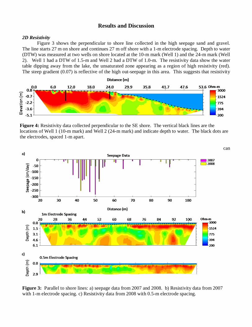
Results and Discussion 2D Resistivity Figure 3 shows the perpendicular to shore line collected in the high seepage sand and gravel. The line starts 27 m on shore and continues 27 m off shore with a 1-m electrode spacing. Depth to water (DTW) was measured at two wells on shore located at the 10-m mark (Well 1) and the 24-m mark (Well 2). Well 1 had a DTW of 1.5-m and Well 2 had a DTW of 1.0-m. The resistivity data show the water table dipping away from the lake, the unsaturated zone appearing as a region of high resistivity (red). The steep gradient (0.07) is reflective of the high out-seepage in this area. This suggests that resistivity

can

Figure 4: Resistivity data collected perpendicular to the SE shore. The vertical black lines are the locations of Well 1 (10-m mark) and Well 2 (24-m mark) and indicate depth to water. The black dots are the electrodes, spaced 1-m apart.

Figure 3: Parallel to shore lines: a) seepage data from 2007 and 2008. b) Resistivity data from 2007 with 1-m electrode spacing. c) Resistivity data from 2008 with 0.5-m electrode spacing.

identify whether there is out-seepage or in-seepage at a given shore location prior to any seepage measurements. Resistivity could also broadly delineate the high and low-seepage zones. Figure 4 shows two 80-m parallel-to-shore lines and the corresponding seepage data. Resistivity data collected using a 0.5-m electrode spacing were compared with data collected the previous year using 1-m electrode spacing. Both data sets show the transition from high-seepage glacial outwash, to low-seepage glacial till, demonstrating reproducibility. However, even the finer 0.5-m electrode spacing was insufficient to resolve the heterogeneity well enough to predict seepage variability within each zone. This variability points to sinuous flow paths, and in such heterogeneous materials the goal of predicting the precise location of high-seepage is especially challenging. The next logical step was to employ 3D surveys once a broad zone of seepage had been identified to attempt to image these pathways.

Figure 5: Horizontal resistivity slice in the till at a depth of 0.7-m with corresponding seepage values. The black dots are seepage meter locations.

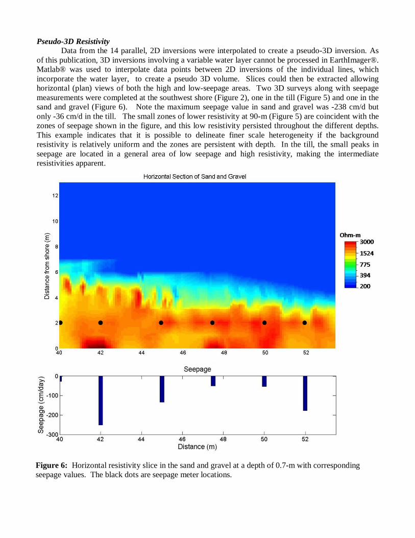
Pseudo-3D Resistivity Data from the 14 parallel, 2D inversions were interpolated to create a pseudo-3D inversion. As of this publication, 3D inversions involving a variable water layer cannot be processed in EarthImager®. Matlab® was used to interpolate data points between 2D inversions of the individual lines, which incorporate the water layer, to create a pseudo 3D volume. Slices could then be extracted allowing horizontal (plan) views of both the high and low-seepage areas. Two 3D surveys along with seepage measurements were completed at the southwest shore (Figure 2), one in the till (Figure 5) and one in the sand and gravel (Figure 6). Note the maximum seepage value in sand and gravel was -238 cm/d but only -36 cm/d in the till. The small zones of lower resistivity at 90-m (Figure 5) are coincident with the zones of seepage shown in the figure, and this low resistivity persisted throughout the different depths. This example indicates that it is possible to delineate finer scale heterogeneity if the background resistivity is relatively uniform and the zones are persistent with depth. In the till, the small peaks in seepage are located in a general area of low seepage and high resistivity, making the intermediate resistivities apparent.

Figure 6: Horizontal resistivity slice in the sand and gravel at a depth of 0.7-m with corresponding seepage values. The black dots are seepage meter locations.

In the sand and gravel (Figure 6), the intermediate resistivity values are seen across the entire section, following the general trend of the long line (Figure 4) previously discussed. The variation in resistivities across the zone makes it difficult to pinpoint an exact seepage location where there are high seepage areas caused by a higher porosity/permeability material. These results show that even 3D resistivity may only be useful in pinpointing seepage in zones where there is a seepage spike associated with of an isolated heterogeneity.

Conclusions

Our work at Mirror Lake showed that broad zones of seepage can be located using 2D resistivity and that the data are reproducible between years. Resistivity can also delineate the gradient of the water table, indicating the direction of seepage for various sections of the shoreline. The employment of 3D resistivity to delineate fine scale heterogeneity proved to be more useful in areas of more uniform resistivity where it is easier to pick out a seepage outlier by locating an unusually conductive path. However, only pseudo-3D sections based on interpolated 2D data inversions were examined here, so the full power of a true 3D inversion for this application is yet to be determined.

Acknowledgements This work was supported by the National Science Foundation Hydrologic Sciences Program under Award No. 0609827. Thanks to the Hubbard Brook Research Foundation for providing logistical support.

Authors’ Note

Any use of trade, product, or firm names is for descriptive purposes only and does not imply endorsement by the U.S. government.

References Chambers, J.E., Ogilvy, R.D., Kuras, O., Cripps, J.C., and Meldrum, P.I., 2002, 3D electrical imaging of known targets at a controlled environmental test site, Environmental Geology, Vol. 41, pp. 690-704. Cherkauer, D.S., 1991, Geophysical mapping of pathways for entry of contaminated ground water to lakes and rivers: Application in the North American great lakes, Hydrological Science and Technology American Institute of Hydrology, Vol. 7, pp. 35-44. Cherkauer, D. S. and Carlson, D. A., 1997, Interaction of Lake Michigan with a Layered Aquifer Stressed by Drainage, Ground Water, Vol. 35, Issue 6, pp. 981-989. Ellefsen, K.J., Hsieh, P. A., Shapiro, A.M., 2002, Crosswell seismic investigation of hydraulically conductive, fractured bedrock near Mirror Lake, New Hampshire, Journal of Applied Geophysics, Vol. 50, pp. 299-317. Gharibi, M. and Bentley, L.R., 2005, Resolution of 3-D electrical resistivity images from inversions of 2-D orthogonal lines, Journal of Environmental and Engineering Geophysics, Vol. 10, Issue 4, pp. 339-349. Heaney, M.J., Nyquist, J.E., Toran, L.E., 2006, Marine Resistivity as a Tool for Characterizing Zones of Seepage at Lake Lacawac, PA, Symposium for the Application of Geophysics to Engineering and Environmental Problems (SAGEEP ’07), pp. 704-711.

Johnson, C.D., 1999, Effects of lithology and fracture characteristics on hydraulic properties in crystalline rocks; Mirror lake research site, Grafton County, New Hampshire, Water Resource investigations, U.S. Geol. Survey, pp. 795-802 Kalbus, E., Reinstorf, K. F., and Schirmer, M., 2006, Measuring methods for groundwater-surface water interactions: a review, Hyrdrol. Earth Syst. Sci., Vol. 10, pp. 873-887. Lee, David Robert., 1977, A Device For Measuring Seepage Flux in lakes and Estuaries, Limnology and Oceanography, Vol. 22, No. 1, pp.140-147. Mitchell, N.M., Nyquist, J.E., Toran, L.E., Rosenberry, D.O., Mikochik, J.S., 2008, Electrical resistivity as a tool for identifying geologic heterogeneities which control seepage at Mirror Lake, NH, Proceeding of the Symposium for the Application of Geophysics to Environmental and Engineering Problems (SAGEEP, 2008), pp. 749-759. Moeller, R. E., 1975, Hydrophyte biomass and community structure in a small oligotrophic New

Hampshire lake, Verhandlungen Internationale Vereinigung Limnologie, Vol. 19, pp. 1004-1012.

Rosenberry, D.O., 2005, Integrating seepage heterogeneity with the use of ganged seepage meters, Limnology and Oceanography: Methods, Vol. 3, pp. 131-142. Rosenberry, D.O. and Winter, T.C., 1993, The significance of fracture flow to the water balance of a lake of fractured crystalline rock terrain, Memoirs of the 24th congress of International Association of Hydrologists, Oslo. Schneider, R.L., Negley, T.L., Wafer, C., 2005, Factors influencing groundwater seepage in a large mesotrophic lake in New York, Journal of Hydrology, Vol. 310, pp. 1-16. Sophocleous, Marios, 2002, Interactions between groundwater and surface water: the state of the science, Hydrogeology Journal, Vol. 10, pp. 52-67. Winter, T.C., 2000, Interaction of ground water and surface water, Proceedings of the Ground- water/Surface-Water Interactions Workshop. Winter, T.C., Rosenberry, D.O., LaBaugh, J.W., 2003, Where does the water in a small watershed come from, Ground Water, Vol. 41, No. 7, pp. 989-1000. Yang, X. and Lagmanson, M., 2006, Comparison of 2D and 3D electrical resistivity imaging methods, Proceeding of the Symposium for the Application of Geophysics to Environmental and Engineering Problems (SAGEEP, 2006), pp. 585-59.