assessment of food chain pathway parameters in biosphere
TRANSCRIPT

PNNL-14955
Prepared for the U.S. Department of Energy under Contract DE-AC05-76RL01830
Assessment of Food Chain Pathway Parameters in Biosphere Models
Annual Progress Report for Fiscal Year 2004
B.A. Napier D.A. Cataldo K.M. Krupka M.M. Valenta R.J. Fellows T.J. Gilmore November 2004

DISCLAIMER This report was prepared as an account of work sponsored by an agency of the United States Government. Neither the United States Government nor any agency thereof, nor Battelle Memorial Institute, nor any of their employees, makes any warranty, express or implied, or assumes any legal liability or responsibility for the accuracy, completeness, or usefulness of any information, apparatus, product, or process disclosed, or represents that its use would not infringe privately owned rights. Reference herein to any specific commercial product, process, or service by trade name, trademark, manufacturer, or otherwise does not necessarily constitute or imply its endorsement, recommendation, or favoring by the United States Government or any agency thereof, or Battelle Memorial Institute. The views and opinions of authors expressed herein do not necessarily state or reflect those of the United States Government or any agency thereof. PACIFIC NORTHWEST NATIONAL LABORATORY operated by BATTELLE for the UNITED STATES DEPARTMENT OF ENERGY under Contract DE-AC05-76RL01830 Printed in the United States of America Available to DOE and DOE contractors from the Office of Scientific and Technical Information,
P.O. Box 62, Oak Ridge, TN 37831-0062; ph: (865) 576-8401 fax: (865) 576-5728
email: [email protected] Available to the public from the National Technical Information Service, U.S. Department of Commerce, 5285 Port Royal Rd., Springfield, VA 22161
ph: (800) 553-6847 fax: (703) 605-6900
email: [email protected] online ordering: http://www.ntis.gov/ordering.htm
This document was printed on recycled paper.
(9/2003)

Technical Letter ReportPNNL-14955
Assessment of Food Chain Pathway Parameters inBiosphere Models
Annual Progress Report for Fiscal Year 2004
Prepared by:B.A. NapierK.M. KrupkaR.J. FellowsD.A. CataldoM.M. ValentaT.J. Gilmore
30 November 2004
Prepared byPacific Northwest National LaboratoryRichland, WA 99352
P. R. Reed, NRC Project Manager
Prepared forDivision of Systems Analysis and Regulatory EffectivenessOffice of Nuclear Regulatory ResearchU. S. Nuclear Regulatory CommissionWashington, DC 20555-0001NRC Job Code Y6469

ii
Abstract
This Annual Progress Report describes the work performed and summarizes some ofthe key observations to date on the U.S. Nuclear Regulatory Commission’s project Assessment of Food Chain Pathway Parameters in Biosphere Models, which wasestablished to assess and evaluate a number of key parameters used in the food-chainmodels used in performance assessments of radioactive waste disposal facilities. Section2 of this report describes activities undertaken to collect samples of soils from threeregions of the United States, the Southeast, Northwest, and Southwest, and performanalyses to characterize their physical and chemical properties. Section 3 summarizesinformation gathered regarding agricultural practices and common and unusual cropsgrown in each of these three areas. Section 4 describes progress in studying radionuclideuptake in several representative crops from the three soil types in controlled laboratoryconditions. Section 5 describes a range of international coordination activitiesundertaken by Project staff in order to support the underlying data needs of the Project.Section 6 provides a very brief summary of the status of the GENII Version 2 computerprogram, which is a “client” of the types of data being generated by the Project, and for which the Project will be providing training to the US NRC staff in the coming FiscalYear. Several appendices provide additional supporting information.

iii
Contents
1.0 Introduction................................................................................................................ 1-12.0 Sampling And Analysis of Groundwater and Soil Samples ...................................... 2-1
2.1 Sampling Sites for Groundwater and Soil Samples............................................... 2-12.2 Methods for Analysis and Characterization of Groundwater and Soil Samples ... 2-62.3 Results of Analyses and Characterization of Groundwater and Soil Samples .... 2-102.4 References for Section 2 ...................................................................................... 2-26
3.0 Agricultural Practices at the 3 Sites ........................................................................... 3-13.1 Washington ............................................................................................................ 3-13.2 Nevada ................................................................................................................... 3-53.3 South Carolina ..................................................................................................... 3-103.4 References for Section 3 ...................................................................................... 3-17
4.0 Plant Studies............................................................................................................... 4-14.1 Introduction............................................................................................................ 4-14.2 Material and Methods ............................................................................................ 4-2
4.2.1 Soil Uptake Experiment................................................................................. 4-24.2.2 Leaf Absorption and Translocation ............................................................... 4-7
4.3 Results and Discussion .......................................................................................... 4-84.3.1 Plant Growth in Differing Soil Types............................................................ 4-94.3.2 Technetium Uptake and Distribution........................................................... 4-114.3.3 Leaf Abrasion Studies.................................................................................. 4-13
5.0 International Coordination and Collaboration ........................................................... 5-15.1 International Atomic Energy Agency .................................................................... 5-15.2 Kazakhstan............................................................................................................. 5-45.3 Russia..................................................................................................................... 5-8
6.0 Status of the GENII Version 2 Computer Code......................................................... 6-16.1 GENII-related References:..................................................................................... 6-3
Appendix A........................................................................................................................... A-1Appendix B ............................................................................................................................B-1

iv
Acknowledgements
The authors are particularly grateful for the technical guidance, review, andencouragement provided by Phillip R. Reed of the U.S. Nuclear Regulatory Commission.The authors would like to thank S.R. Baum, K.M. Geiszler, I.V. Kutnyakov, V.L.LeGore, M.J. Lindberg, H.T. Schaef, and T.S Vickerman (all of PNNL) for assistingwith various aspects of the analyses and characterization of the groundwater and soilsamples. We would also like to thank R.J. Serne, W.J. Deutsch, and their PNNLcoworkers for providing written descriptions of the methods used for analysis andcharacterization of the groundwater and soil samples.

v
Acronyms
ASA American Society of AgronomyASTM American Society for Testing and MaterialsCEC cation exchange capacitycpm counts per minutecps counts per secondDDI distilled deionized (water)DOE U.S. Department of EnergyDUP duplicate sampleEPA U.S. Environmental Protection AgencyICP-MS inductively coupled plasma-mass spectroscopy (spectrometer)ICP-OES inductively coupled plasma-optical emission spectroscopy (same as
ICP-AES)ICDD International Center for Diffraction Data, Newtown Square, PennsylvaniaIRSE Institute of Radiation Safety and Ecology, Kurchatov, KazakhstanISTC International Science and Technology CenterJCPDS Joint Committee on Powder Diffraction StandardsMPA Mayak Production Association, Ozersk, RussiaND not detectedPDF™ powder diffraction filePNNL Pacific Northwest National LaboratoryQA quality assuranceSTS Semipalatinsk Test Site, KazakhstanUSGS U.S. Geological SurveyXRD X-ray powder diffractometry analysis (commonly called X-ray diffraction)XRF X-ray fluorescence analysis
vi
Units of Measure
Å angstromg gramL literM molarity, mol/Lmg milligrammL milliliterN Normality (of a solution), in number of gram equivalent weights of solute
per liter of solutionI/Io relative intensity of an XRD peak to the most intense peakwt% weight percentºC temperature in degrees Celsius [T(ºC) = T(K)–273.15)λ wavelength micro (prefix, 10-6)eq microequivalentg microgramm micrometerθ angle of incidence (Bragg angle)

1-1
1.0 Introduction
The U.S. Nuclear Regulatory Commission’s project Assessment of Food Chain PathwayParameters in Biosphere Models has been established to assess and evaluate a number ofkey parameters used in the food-chain models used in performance assessments ofradioactive waste disposal facilities. The objectives of the research program are to:
Provide data and information for the important features, events, and processes ofthe pathway models for use in biosphere computer codes. These codes calculatethe total effective dose equivalent (TEDE) to the average member of the criticalgroup and maximally exposed individual. This exposure is for the referencebiosphere from radionuclides in the contaminated ground water release scenariosin NRC's performance assessments of waste disposal facilities anddecommissioning sites,
Reduce uncertainties in food-chain pathway analysis from the agriculture scenariosof biosphere models in performance assessment calculations,
Provide better data and information for food-chain pathway analyses by:o Performing laboratory and field experiments, including integral and
separate effect experiments, to evaluate the potential pathways and uptakemechanisms of plants and animals contaminated by long-livedradionuclides,
o Presenting food-chain pathway data and information by regional and localgeographical locations,
o Quantifying uncertainties in the radioactive contamination of food cropsand long-term build up of radionuclides in soils with contaminated groundwater from water irrigation systems,
o Determining data on factors affecting radionuclide uptake of food cropsincluding irrigation water processes, soil physical and chemical properties,soil leaching and retention properties near crop roots, soil resuspensionfactors and other soil and plant characteristics,
o Obtaining experimental data in both deterministic and as probabilisticdistributions,
o Determining food-chain pathway data and information for a prioritized listof radionuclides:
Review and evaluate data and information published by the international scientificcommunity on food-chain pathway issues.
The results of this research program will provide needed food-chain and animalproduct pathway data and information for important radionuclides that will be used bythe NRC staff to assess dose to persons in the reference biosphere (e.g., persons who liveand work in an area potentially affected by radionuclide releases) of waste disposalfacilities and decommissioning sites. Data from this research program are expected to beused in biosphere models to calculate the dose from ground water release scenarios inperformance assessment computer codes.

1-2
In Fiscal Year 2004, efforts were undertaken on most of these objectives. This AnnualProgress Report describes the work performed and summarizes some of the keyobservations to date.
Section 2 of this report describes activities undertaken to collect samples of soils fromthree regions of the United States, the Southeast, Northwest, and Southwest, and performanalyses to characterize their physical and chemical properties. Section 3 summarizesinformation gathered regarding agricultural practices and common and unusual cropsgrown in each of these three areas. Section 4 describes progress in studying radionuclideuptake in several representative crops from the three soil types in controlled laboratoryconditions. Section 5 describes a range of international coordination activitiesundertaken by Project staff in order to support the underlying data needs of the Project.Section 6 provides a very brief summary of the status of the GENII Version 2 computerprogram, which is a “client” of the types of data being generated by the Project, and forwhich the Project will be providing training to the US NRC staff in the coming FiscalYear. Several appendices provide additional supporting information.

2-1
2.0 Sampling and Analysis of Groundwater and Soil Samples
Uncontaminated soil and groundwater samples were collected from 3 sites that are in thevicinity of waste disposal facilities of interest to NRC and unaffected by disposalactivities at those sites. The soil and groundwater samples were collected for use inTask 4 for the plant radionuclide uptake studies. The areas for sampling includecurrently operating and proposed waste disposal facilities and decommissioning sites,including the commercial low-level radioactive waste (LLW) sites in the states ofWashington and South Carolina.
2.1 Sampling Sites for Groundwater and Soil Samples
Three areas for soil and water samples were identified that met the objectives identifiedin the work plan for the “Assessment of Food Chain Pathway Parameters in Biosphere Models” project. These sites include the Hanford Site, Washington; Savannah River,South Carolina; and Nye County, Nevada. These sites are each located near a current orproposed nuclear waste disposal facility or decommissioning site, and together provide arange of soil characteristics for the radionuclide biouptake studies.
The experimental design of the uptake experiments requires approximately 300 litersof water and 0.2 cubic meters of soil from each site. The latitude and longitude positionof each sampling location was recorded by using a global positioning system (GPS) unitto provide traceability and the opportunity to provide duplicate samples if required. Inaddition, at the one privately owned site in Nye County, Nevada, it was arranged throughan agreement with the landowner that the site would be available for re-sampling shouldany additional material be needed.
2.1.1 Hanford Site, Washington
The sampling site for the Hanford soil and groundwater samples is located offWashington highway 240 nearthe area referred to as the “Yakima Barricade” at the western entrance to the U.S. Department of Energy Hanford Site in southeasternWashington State. Logistically, the sample site is easily assessable by road, and a pumpis installed in the well used for groundwater sampling (Figure 2.1). The Hanford Sitedesignation for the well is 699-49-100C, and the coordinates are North 46.577,West 119.726. The well has been used in the past for providing water to the guard shackat the Yakima Barricade (see structure in background at top of right photograph in Figure2.1), and is still used to provide “up-gradient background” groundwater samples (i.e., water not affected by Hanford disposal activities) to the Hanford Site environmentalprograms. The water chemistry of the well has been well characterized, and the analysesare available through the Hanford Environmental Information System (HEIS) data base.

2-2
The Hanford soil1 sample was collected within 100 m of the well used for thegroundwater sample, and the coordinates for the location of the soil sample areNorth 46.5757, West 119.7259. The soil sample is a silty, very fine sand that is referredto as the McGee Ranch soil. The soil in this area has been extensively characterized,because there are plans to use this sediment as a soil covering for surface barriers onwaste-disposal areas at the Hanford Site (Bechtel Hanford 2002) (Figure 2.1).
Groundwater Sampling Soil Sampling
Figure 2.1. Locations of Groundwater and Soil Samples from the Hanford Site
2.1.2 Nye County, Nevada
The sampling site (Figure 2.2) in Nye County is located in a desert valley approximately110 miles west of Las Vegas in the Amargosa Valley, Nevada. The soil and groundwatersamples were collected from private land owned by Dave Rau. To get to the site, onemust travel west from Las Vegas approximately 110 miles on Nevada highway 95. Atthe junction of highways 95 and 373, go south for 10 miles to Mecca Road, and then turnwest and go 5.5 miles to Van Patton Drive. At this junction, one then turns south andgoes to the third driveway on the west side which has the address 1658 Van Patton Drive.
1 Because of its depositional history, the unconsolidated surface and near-surface geologic material atthe Hanford Siteis referred to as a “sediment” in Hanford Site literature.

2-3
The groundwater was collected from an irrigation well that is used to flood irrigatedpastureland. The coordinates for the well used for the groundwater sample areNorth 36 29' 24.4", West 116 30' 51.5". The pasture was used to grow alfalfa for about14 years up until about 1996, when it was allowed to turn to pasture. According to theland owner, the soil was originally conditioned using approximately 10 tons/acre ofgypsum. No commercial fertilizer was used on the pasture.
The soil was approximately 2.5 feet thick at the sample site, and consists of a lightbrown silty sand. The coordinates for the site of the soil sample are North 36 29' 23.7",West 116 30' 52.0". Near the base, the occurrence of white streaks in the soil increaseduntil the soil transitioned into broken-up calcrete.
Figure 2.2. Location in Nye County, Nevada WhereGroundwater and Soil Samples were Collected
2.1.3 Savannah River Site, South Carolina
This site was selected because this soil provides a good representation of forest soil fromthe southeastern United States. PNNL staff also had contacts at the U.S. Department ofEnergy Savannah River Site who could cost-effectively provide uncontaminatedgroundwater and soil samples from this location. This site receives considerably moreinfiltration from rainfall and snowmelt, and has a soil that is expected to have a higherorganic carbon content than the soil samples from Hanford and Nye County. The watersamples are from well HSB-85A (Figure 2.3) at coordinates North 33 17' 6.548", West 8139' 17.7448". The soil samples were collected near well MSB 21 TA (Figure 2.4) at

2-4
coordinates North 33 19' 58.31", West 81 44' 39.2". The groundwater and soil sampleswere provided by J. Rossabi, who at that time worked at the Savannah River TechnologyCenter in Aiken, South Carolina. The locations selected for the groundwater and soilsamplesrepresent “clean” groundwater and soil, which donot contain any radionuclidecontamination at concentrations above natural background levels. Also, each samplinglocation has background data associated with it that was collected as part of theenvironmental monitoring program at the Savannah River Site.
Figure 2.3. Well Used for Groundwater Sample from Savannah River Site

2-5
Figure 2.4. Location Where Soil Sample Collected from Savannah River Site [Soil wassampled from surface (bottom photograph) near the feet of the personstanding in the trees in the top photograph.]

2-6
2.2 Methods for Analysis and Characterization of Groundwater andSoil Samples
The following method descriptions were taken, with the permission of the lead authors,from reports published by the PNNL Applied Geology and Geochemistry Group, such asDeutsch et al. (2004) and Serne et al. (2004).
2.2.1 Analysis of Groundwater Samples
2.2.1.1 pH and Conductivity
The pH values of the groundwater samples from the Hanford Site, Nye County, andSavannah River Site were measured using a solid-state pH electrode and a pH metercalibrated with buffers bracketing the expected range. This measurement is similar toTest Methods for Evaluating Solid Wastes: Physical/Chemical Methods SW-846 9040B(EPA 1995). Electrical conductivity was measured and compared to potassium chloridestandards with a range of 0.001 M to 1.0 M. The pH and conductivity subsamples werefiltered prior to analysis.
2.2.1.2 Alkalinity
The alkalinity of the groundwater samples from the Hanford Site, Nye County, andSavannah River Site were measured using standard titration. A volume of standardizedsulfuric acid (H2SO4) was added to the sample to an endpoint of pH 8.3 and then anendpoint of pH 4.5. The volume of H2SO4 needed to achieve each endpoint is used tocalculate the phenolphthalein (OH- + CO3
2-) and total (OH- + HCO3- + CO3
2-) alkalinityas calcium carbonate (CaCO3). The alkalinity procedure is similar to Standard Method2320 B (Clesceri et al. 1998).
2.2.1.3 Anions
Analyses of dissolved anions in groundwater samples from the Hanford Site, NyeCounty, and Savannah River Site were measured using an ion chromatograph. Bromide,carbonate, chloride, fluoride, nitrate, phosphate, and sulfate were separated on a DionexAS17 column with a gradient elution technique from 1 mM to 35 mM KOH andmeasured using a conductivity detector. This methodology is similar to Method 9056 inTest Methods for Evaluating Solid Wastes: Physical/Chemical Methods EPA SW-846(EPA 1994b) with the exception of using gradient elution with NaOH.

2-7
2.2.1.4 Total Carbon
Total carbon contents of the groundwater samples from the Hanford Site, Nye County,and Savannah River Site were measured using a Shimadzu Carbon analyzer ModelTOC-V csn that is equipped with an autosampler. The method used of measuring thecarbon content of the groundwater samples is described in PNNL Technical ProcedureAGG-TOC-001 (PNNL 2004),2 and is similar to EPA Method 9060 (Total OrganicCarbon) in Test Methods for Evaluating Solid Wastes: Physical/Chemical Methods EPASW-846 (EPA 1986). The adequacy of the system performance was confirmed byanalyzing for known quantities of a liquid carbon standard.
2.2.1.5 Cations and Trace Metals
Analyses of major cations, such as Al, Ca, Fe, K, Mg, Mn, Na, and Si, dissolved in thegroundwater samples from the Hanford Site, Nye County, and Savannah were completedby inductively coupled plasma-optical emission spectroscopy (ICP-OES) (EPA Method6010B, EPA 1996). Trace metals analyses, including Ag, As, Cd, Cr, Mo, Pb, Ru, Se,and U, were completed by inductively coupled plasma-mass spectroscopy (ICP-MS)using a method that is similar to EPA Method 6020 (EPA 1994a). For both ICP-OES andICP-MS, high-purity calibration standards were used to generate calibration curves and toverify continuing calibration during the analysis. Multiple dilutions of selected sampleswere made and analyzed to investigate and correct for matrix interferences. The ICP-MSresults are reported as total element concentration in terms of the specific isotopemeasured. The instrument software converts the concentration of an isotope of anelement to the total concentration of the element based on the distribution of isotopes inthe natural environment. For example, the total Cr concentration is reported from the rawcount rates for both 52Cr and 53Cr isotopes based on taking the raw counts and dividing bythe fraction of 52Cr and 53Cr found in nature to yield estimates of total Cr in the sample.
2.2.2 Characterization and Analysis of Bulk Soil Samples
2.2.2.1 X-ray Diffraction
The primary crystalline minerals present in each bulk soil sample were identified using aScintag X-ray powder diffraction (XRD) unit equipped with a Pelter thermoelectricallycooled detector and a copper X‑ray tube. The diffractometer was operated at 45 kV and40mA. Individual scans were obtained from 2 to 65° 2θ with a dwell time of 2 seconds.Scans were collected electronically and processed using the JADE® XRD pattern-processing software. Identification of the mineral phases in the background-subtractedpatterns was based on a comparison of the XRD patterns measured for the sludge samples
2 PNL. 2004. “PNNL Technical Procedure AGG-TOC-001 [Operating of CarbonAnalyzer (TOC-V + SSM-5000A + ASI (Shimadzu))].” Procedure in review, Pacific Northwest National Laboratory, Richland, Washington.

2-8
with the mineral powder diffraction files (PDF™) published by the Joint Committee on Powder Diffraction Standards (JCPDS) International Center for Diffraction Data (ICDD).
2.2.2.2 Elemental Analysis by X-ray Fluorescence
At the time of this progress report, bulk elemental analysis by X-ray fluorescence (XRF)of the soil samples from the Hanford Site, Nye County, and Savannah River Site were inthe sample queue for completion at the GeoAnalytical Laboratory in the Department ofGeology at the Washington State University, Pullman, Washington. These analyses arebeing completed using an existing service contract that PNNL has established withWashington State University. The XRF analyses were originally going to be done onnew, state-of-the-art XRF instrumentation purchased by the Applied Geology andGeochemistry Group at PNNL. However, delays in its installation, shakedown testing,and approval of its technical operation procedure required that the XRF analyses for thesesoil samples be completed elsewhere. The results of the XRF analyses will be includedin the final project technical report along with the analysis and characterization resultsdescribed in this progress report.
2.2.2.3 Particle Size Distribution
American Society for Testing and Materials (ASTM) procedures ASTM D1140-00(ASTM 2000) (Standard Test Methods for Amount of Material in Soils Finer Than theNo. 200 [75 µm] Sieve) and D422-63 (ASTM 2003a) (Standard Test Method forParticle-Size Analysis of Soils) were used for particle size analysis of the soil samplesfrom the Hanford Site, Nye County, and Savannah River Site. In ASTM D422-63, asedimentation process using a hydrometer is used to determine the distribution of particlesizes smaller than 75 µm, while sieving was used to measure the distribution of particlesizes larger than 53 µm (retained on a No. 270 sieve). A No. 10 sieve, which has sievesize openings of 2.00 mm, was firstused to remove the fraction larger than “very coarse” prior to particle size analysis.
2.2.2.4 Moisture Content
Gravimetric water contents of the soil samples from the Hanford Site, Nye County, andSavannah River Site were determined using PNNL procedure PNL-MA-567-DO-1 (PNL1990).3 This procedure is based on the ASTM Method D2216-98 (Test Method forLaboratory Determination of Water (Moisture) Content of Soil and Rock by Mass)(ASTM 1998). One representative subsample of each soil sample was placed in taredcontainers, weighed, and dried in an oven at 105°C (221°C) until constant weight wasachieved, which took at least 24 hours. The containers then were removed from the oven,sealed, cooled, and weighed. At least two weighings, each after a 24-hour heating, were
3 PNL. 2000. “PNNL Technical Procedure SA-7. Water Content.” Procedure approved in May 2000, in Procedures for Ground-Water Investigations,PNL-MA-567, Pacific Northwest National Laboratory, Richland, Washington.

2-9
performed to ensure that all moisture was removed. The gravimetric water content wascomputed as the percentage change in soil weight before and after oven drying.
2.2.2.5 Cation Exchange Capacity
The cation exchange capacity (CEC) of the soil samples from the Hanford Site, NyeCounty, and Savannah River Site were determined using the method described in ASA(1982). This method is particularly suited to arid land soils, including these containingcarbonate, gypsum, and zeolites, This procedure involves two steps. The first stepconsists of saturation of the cation exchange sites with Na by reaction of the soil with pH8.2, 60% ethanol solution of 0.4-N NaOAc–0.1 N NaCl. This is then followed byextraction of 0.5 N MgNO3. The concentrations of dissolved Na and Cl are thenmeasured in the extracted solution so that the dissolved Na from the excess saturationsolution, carried over from the saturation step to the extraction step, is deducted from thetotal Na. This provides amount of exchangeable Na, which is equivalent to the CEC.
2.2.2.6 Carbon Content
The total carbon and the inorganic carbon contents of the soil samples from the HanfordSite, Nye County, and Savannah River Site were measured using a Shimadzu CarbonAnalyzer Model TOC-V csn. The method used to measure the carbon contents of the soilsamples is described in PNNL Technical Procedure AGG-TOC-001 (PNNL 2004),4 andis similar to ASTM Method E1915-01 (Test Methods for Analysis of Metal Bearing Oresand Related Materials by Combustion Infrared Absorption Spectrometry) (ASTM 2001).Known quantities of calcium carbonate standards were analyzed to verify that theinstrumentation was operating properly. Inorganic carbon content was determinedthrough calculations performed using the microgram per-sample output data and sampleweights. The organic carbon content of the soil samples was calculated by subtractingthe inorganic carbon contents from the respective total carbon contents for each sample.
2.2.2.7 1:1 Soil:Water Extracts
The water-soluble inorganic constituents in the soil samples from the Hanford Site, NyeCounty, and Savannah River Site were determined using a 1:1 soil:deionized-waterextract method. The extracts were prepared by adding an exact weight of deionizedwater to approximately 60 to 80 g of soil subsample. The weight of deionized waterneeded was calculated based on the weight of the field-moist samples and theirpreviously determined moisture contents. The sum of the existing moisture (porewater)and the deionized water was fixed at the mass of the dry soil. The appropriate amount ofdeionized water was added to screw cap jars containing the soil samples. The jars weresealed and briefly shaken by hand, then placed on a mechanical orbital shaker for onehour. The samples were allowed to settle until the supernatant liquid was fairly clear.
4 PNL. 2004. “PNNL Technical Procedure AGG-TOC-001 [Operating of CarbonAnalyzer (TOC-V + SSM-5000A + ASI (Shimadzu))].” Procedure in review, Pacific Northwest National Laboratory, Richland, Washington.

2-10
The supernatant was carefully decanted and separated into unfiltered aliquots forconductivity and pH determinations, and filtered aliquots (passed through 0.45 µmmembranes) for anion, carbon, and cation analyses. More details can be found inRhoades (1996) and within Methods of Soils Analysis - Part 3 (ASA 1996). The methodsused for the pH, conductivity, anion, carbon, and cation analyses are the same as thosedescribed above for the analysis of the groundwater samples. The results for the analysesof the 1:1 soil:water extracts for the three soil samples are reported in terms of both unitsper gram of soil and units per milliliter of pore water. This conversion is based on asoil-to-water ratio of 1.0.
2.3 Results of Analyses and Characterization of Groundwater and SoilSamples
Table 2.1 lists the tables and figures that contain the results of the analyses andcharacterization studies of the groundwater, soil, and 1:1 soil:water extract samples fromthe Hanford Site, Nye County, and Savannah River Site.
In the following tables, analyses are listed for primary and duplicate samples of oneof the three groundwater, soil, and 1:1 soil:water extract samples. A duplicate sample isselected at random when a set of samples is submitted for analyses as part of the standardlaboratory quality-assurance operating procedures used by the analytical laboratories inthe PNNL Applied Geology and Geochemistry Group.
The background-subtracted XRD patterns for the Hanford Site, Nye County, andSavannah River Site soil samples are shown in Figure 2.5, Figure 2.6, and Figure 2.,respectively. Each XRDpattern is shown as a function of degrees 2θ based on CuKαradiation (λ=1.5406 Å). The vertical axis in each pattern represents the intensity incounts per second (cps) of the XRD peaks. In order to conveniently scale the XRDpatterns on the vertical axes and visualize the minor XRD peaks, it was necessary tocutoff the intensity of the most intense XRD peak in each pattern. These intensity cutoffsare labeled on each XRD pattern, and correspond to the largest XRD peak for feldspar forthe Hanford Site soil sample, and for quartz for the Nye County and Savannah River Sitesoil samples.
At the bottom of each XRD pattern, one or more schematic database (PDF) patternsconsidered for phase identification are also shown for comparison purposes. The heightof each line in the schematic PDF patterns represents the relative intensity of an XRDpeak (i.e., the most intense [the highest] peak has a relative intensity [I/Io] of 100%). Asnoted previously, a crystalline phase typically must be present at greater than 5 wt% ofthe total sample mass (greater than 1 wt% under optimum conditions) to be readilydetected by XRD.

2-11
Table 2.1. Tables and Figures Containing the Results of the Analyses andCharacterization Studies of the Groundwater, Soil, and 1:1 Soil:Water ExtractSamples from the Hanford Site, Nye County, and Savannah River Site
Type of Sample Table orFigure Numbers Results Reported
Table 2.2 pH and Conductivity
Table 2.3 Alkalinity at pH 8.3 and 4.5 Endpoints
Table 2.4 Dissolved Anions by IC
Table 2.5 Total Dissolved Carbon
Table 2.6 Dissolved Macro and Trace Elements byICP-OES
Groundwater Samples
Table 2.7 and Table2.8 Dissolved Trace Metals by ICP-MS
Figure 2.5, Figure 2.6,and Figure 2.7
XRD for Hanford Site, Nye County, andSavannah River Site Samples,Respectively
Table 2.9 Particle Size of Bulk Solid
Table 2.10 Moisture Content
Table 2.11 Cation Exchange Capacity (CEC)
Soil Samples
Table 2.12 Contents of Total, Inorganic, and OrganicCarbon
Table 2.13 pH and Conductivity
Table 2.14 Alkalinity at pH 8.3 and 4.5 Endpoints
Table 2.15 Dissolved Anions by IC
Table 2.16 and Table2.17
Dissolved Macro and Trace Elements byICP-OES
1:1 Soil:Water Extracts
Table 2.18 and Table2.19 Dissolved Trace Metals by ICP-MS
The following minerals were identified in the soil samples (see Figure 2.5, Figure 2.6,and Figure 2.):
Hanford Site soil–quartz, plagioclase feldspar, microcline feldspar, amphibole,chlorite, and mica
Nye County soil - quartz, plagioclase feldspar, microcline feldspar, amphibole,zeolite, and mica
Savannah River Site soil - quartz

2-12
More detailed analyses would be required to refine the identities of the general mineralidentifications (e.g., plagioclase, amphibole, zeolite, mica, etc.) to specific compositions.The soil sample from Nye County appears to contain a zeolite mineral. Although thepattern for this soil sample (Figure 2.) was a good match to the database pattern forclinoptilolite (PDF 47-1870), other compositions of zeolites may also match this pattern.Several reflections (i.e., 16.62, 25.50, and 33.44 °2θ) in the XRD pattern for soil from the Savannah River Site could not be identified. Additional XRD patterns measured atslower scanning rates would be needed to identify the minerals associated with thesereflections.
Table 2.2. pH and Conductivity Values for the Groundwater Samples
Groundwater Samples pH Conductivity(mS/cm)
Hanford Site 8.43 0.544Hanford Site (duplicate) 8.35 0.543Nye County 8.42 0.197Savannah River Site 8.75 1.052
Table 2.3. Alkalinity Values for the Groundwater Samples
Alkalinity atpH 8.3 Endpoint
Total Alkalinity atpH 4.5 EndpointGroundwater Samples
(mg CaCO3/L)Hanford Site 0.0* 168.36
Hanford Site (duplicate) 0.0 167.63Nye County 15.372 290.60Savannah River Site 0.0 81.984* Alkalinity values of 0.0 mg CaCO3/L at the pH 8.3 endpoint indicate that
the starting pH values of the respective groundwater samples were near orless than pH 8.3.

2-13
Table 2.4. Concentrations of Dissolved Anions in the Groundwater Samples
Br- CO32- Cl- F- NO3
- PO43- SO4
2-GroundwaterSamples
(µg/mL)Hanford Site <0.48 222.7 20.07 0.42 13.76 <0.51 79.75
Hanford Site(duplicate)
<0.48 220.9 20.00 0.42 13.66 <0.51 79.49
Nye County <0.48 389.1 44.96 5.91 2.47 <0.51 187.0
Savannah River Site <0.48 59.38 2.60 0.09 <0.43 <0.51 5.29
Table 2.5. Concentrations of Total Dissolved Carbon in the Groundwater Samples
Total Dissolved CarbonGroundwater Samples
#1 #2 Average
(mg/L)Hanford Site 39.85 40.14 40.00Nye County 68.40 68.33 68.37Savannah River Site 17.83 17.74 17.79

2-14
Table 2.6. Concentrations of Dissolved Macro and Trace Metals in the GroundwaterSamples as Determined by ICP-OES
Al As B Ba Be Bi Ca Cd Co CrGroundwaterSamples
(µg/L)
Hanford Site ND <1.3E+02 <1.3E+02 1.8E+02 <6.3E+01 ND 5.8E+04 ND <2.5E+01 <6.3E+01Hanford Site(duplicate) ND <1.3E+02 <1.3E+02 1.5E+02 <6.3E+01 ND 5.9E+04 ND <2.5E+01 <6.3E+01
Nye County ND <1.3E+02 8.8E+02 8.1E+01 <6.3E+01 ND 1.9E+04 ND <2.5E+01 <6.3E+01Savannah RiverSite ND <1.3E+02 <1.3E+02 6.3E+01 <6.3E+01 ND 3.3E+04 ND ND <6.3E+01
Cu Fe K Li Mg Mn Mo Na Ni P
(µg/L)
Hanford Site <2.5E+02 <2.5E+01 7.6E+03 <2.5E+03 2.2E+04 ND <2.5E+01 2.4E+04 <2.5E+01 <3.1E+02
Hanford Site(duplicate) <2.5E+02 <2.5E+01 7.7E+03 <2.5E+03 2.2E+04 ND ND 2.4E+04 <2.5E+01 <3.1E+02
Nye County <2.5E+02 <2.5E+01 1.4E+04 <2.5E+03 1.7E+04 ND <2.5E+01 2.1E+05 <2.5E+01 <3.1E+02Savannah RiverSite <2.5E+02 <2.5E+01 <1.3E+03 <2.5E+03 8.2E+02 ND <2.5E+01 1.7E+03 <2.5E+01 <3.1E+02
Pb S Se Si Sr Ti Tl V Zn Zr
(µg/L)
Hanford Site ND ND <5.0E+02 2.9E+04 2.3E+02 ND ND <2.5E+02 3.7E+02 <2.5E+01
Hanford Site(duplicate) ND ND <5.0E+02 2.9E+04 2.3E+02 ND ND <2.5E+02 3.5E+02 ND
Nye County ND ND <5.0E+02 2.2E+04 5.3E+02 ND ND ND <6.3E+01 ND
Savannah RiverSite ND ND <5.0E+02 1.3E+04 8.5E+01 ND ND <2.5E+02 <6.3E+01 <2.5E+01

2-15
Table 2.7. Concentrations of Dissolved Trace Metals in the Groundwater Samples asDetermined by ICP-MS
Ag –total based on As –totalbased on Cd –total based on Cr –total based on
107Ag 109Ag 75As 111Cd 114Cd 52Cr 53CrGroundwater
Samples
(µg/L)
Hanford Site <1.25E-01 <1.25E-01 2.51E+00 <5.00E-01 <5.00E-02 2.05E+00 2.24E+00Hanford Site(duplicate) <1.25E-01 <1.25E-01 2.85E+00 <5.00E-01 <5.00E-02 1.99E+00 2.55E+00
Nye County <1.25E-01 <1.25E-01 4.02E+01 <5.00E-01 <5.00E-02 <1.25E+00 1.53E+00
Savannah River Site <1.25E-01 <1.25E-01 <2.50E+00 <5.00E-01 <5.00E-02 <1.25E+00 1.28E+00
Table 2.8. Concentrations of Dissolved Trace Metals in the Groundwater Samples asDetermined by ICP-MS (Continued)
Mo –total based on Pb –total based on Ru –total based on Se –totalbased on
U –totalbased on
95Mo 98Mo 206Pb 208Pb 101Ru 102Ru 82Se 238UGroundwater
Samples
(µg/L)
Hanford Site <2.50E+00 1.26E+00 <1.25E+00 <1.25E+00 <1.25E+00 <1.25E+00 <2.50E+01 2.32E+00Hanford Site(duplicate) <2.50E+00 <1.25E+00 <1.25E+00 <1.25E+00 <1.25E+00 <1.25E+00 <2.50E+01 2.30E+00
Nye County 1.34E+01 1.24E+01 <1.25E+00 <1.25E+00 <1.25E+00 <1.25E+00 <2.50E+01 3.78E+00
Savannah River Site <2.50E+00 <1.25E+00 <1.25E+00 1.32E+00 <1.25E+00 <1.25E+00 <2.50E+01 <5.00E-02

2-16
Figure 2.5. Background-Subtracted XRD Pattern for Hanford Site Soil Sample
5 10 15 20 25 30 35 40 45 50 55 60 65
Rel
ativ
eIn
tens
ity(c
ps) Hanford Site
Soil Sample
QuartzPlagioclase
MicroclineAmphibole
Mica
Chlorite
Intensity Cutoff

2-17
Figure 2.6. Background-Subtracted XRD Pattern for Nye County Soil Sample
5 10 15 20 25 30 35 40 45 50 55 60 65
Rel
ativ
eIn
tens
ity(c
ps)
Nye CountySoil Sample
Quartz
PlagioclaseMicroclineAmphibole
Mica
Zeolite
Intensity Cutoff

2-18
Figure 2.7. Background-Subtracted XRD Pattern for Savannah River Site Soil Sample
5 10 15 20 25 30 35 40 45 50 55 60 65
Rel
ativ
eIn
tens
ity(c
ps) Savannah River Site
Soil Sample
Quartz
Intensity Cutoff

2-19
Table 2.9. Particle Size Analysis of the Bulk Soil Samples
Gravel(x > 2 mm)
Sand(2 > x > 0.050 mm)
Silt/Clay(x < 0.050 mm)Soil Samples
(wt%)Hanford Site 0.0 82.92 17.08Nye County 0.0 98.99 1.01Savannah River Site 0.0 97.01 2.99
Table 2.10. Moisture Contents of the Bulk Soil Samples
Moisture (wt%)Soils
FirstWeighing
SecondWeighing
Hanford Site 2.49 2.39Nye County 2.51 2.30Nye County (duplicate) 2.57 2.38Savannah River Site 0.25 0.21
Table 2.11. Cation Exchange Capacity (CEC) Values for the Soil Samples
CEC (meq/100 g)Soils#1 #2 #3 Average
Hanford Site 38.2 35.1 ND* 36.7Nye County 27.3 28.5 29.3 28.4Savannah River Site 26.8 22.4 ND* 24.6* ND–Third analysis of CEC not determined for these soil samples.

2-20
Table 2.12. Carbon Contents of the Soil Samples
Total Carbon Total InorganicCarbon
TotalInorganicCarbon As
CaCO3
Total OrganicCarbon
(by difference)
#1 #2 Ave #1 #2 Ave Ave Ave
Soil
(wt%)
Hanford Site 0.36 0.36 0.36 0.09 0.09 0.09 0.72 0.27Nye County 1.10 1.08 1.09 0.97 0.98 0.97 8.11 0.12Nye County(duplicate) 1.38 1.38 1.38 1.26 1.22 1.24 10.31 0.14
Savannah RiverSite 0.63 0.63 0.63 0.0 0.0 0.0 0.0 0.63
Table 2.13. pH and Conductivity Values for the 1:1 Soil:Water Extracts
1:1 Soil:Water Extracts pH Conductivity(mS/cm)
Conductivity (mS/cm)Dilution Corrected (in
Pore Water)
Hanford Site 7.48 0.184 7.38
Nye County 8.07 0.400 15.94
Nye County (duplicate) 8.14 0.407 15.85
Savannah River Site 4.46 0.303 120.90
Table 2.14. Alkalinity Values for the 1:1 Soil:Water Extracts
Akalinity atpH 8.3 Endpoint
Total Alkalinity atpH 4.5 Endpoint
Porewater Total Alkalinityat pH 4.5 EndpointDilution Corrected
(in Pore Water)
1:1 Soil:WaterExtracts
(mg CaCO3/L)
Hanford Site 0.0* 85.644 3436.0
Nye County 6.588 137.61 5485.7
Nye County (duplicate) 5.124 142.74 5557.3
Savannah River Site 0.0* 10.248 4088.9
* Alkalinity values of 0.0 mg CaCO3/L at the pH 8.3 endpoint indicate that the starting pH valuesof the respective extract samples were near or less than pH 8.3.

2-21
Table 2.15. Concentrations of Dissolved Anions in 1:1 Soil:Water Extract
Br- CO32- Cl- F- NO3
- SO42-
1:1 Soil:WaterExtracts
(µg/g soil)
Hanford Site <0.48 70.36 <0.236 0.16 2.50 1.36
Nye County <0.48 161.8 6.86 7.03 5.57 30.81
Nye County (duplicate) <0.48 162.0 6.92 7.07 5.20 30.69
Savannah River Site <0.48 <50.00 2.85 5.53 2.22 29.22
(µg/mL pore water)
Hanford Site <19.30 2,823 <9.452 6.62 100.3 54.63
Nye County <19.17 6,446 273.5 280.4 222.0 1,228
Nye County (duplicate) <18.73 6,307 269.5 275.2 202.3 1,195
Savannah River Site <191.9 <19,950 1,136 2,205 886.8 11,660
See dilution factors in another table–40.12, 39.86, 38.93, and 399.00Dilution factor corrected - µg in water extract per mL Pore Water

2-22
Table 2.16. Concentrations (µg/g soil) of Dissolved Macro and Trace Metals in the 1:1Water Extracts as Determined by ICP-OES
Al As B Ba Be Bi Ca Cd Co Cr1:1Soil:Water
Extracts (µg/g soil)
Hanford Site ND ND <2.5E+02 <1.2E-01 <2.5E-01 <1.2E+00 2.10E+01 ND <6.2E-01 <1.2E-01
Nye County <5.0E-01 ND <2.5E+02 <1.3E-01 <2.5E-01 <1.3E+00 5.40E+00 ND <6.3E-01 <1.3E-01Nye County(duplicate) <5.0E-01 <5.0E+00 <2.5E+02 <1.3E-01 <2.5E-01 <1.3E+00 5.64E+00 ND <6.3E-01 <1.3E-01
SavannahRiver Site 1.23E+01 ND <2.5E+02 4.20E-01 <2.5E-01 <1.2E+00 1.98E+01 ND <6.2E-01 <1.2E-01
Cu Fe K Li Mg Mn Mo Na Ni P
(µg/g soil)
Hanford Site <2.5E+00 <5.0E-01 <6.2E+01 <1.2E+00 5.19E+00 ND <2.5E-01 <2.5E+00 <1.2E+00 <6.2E+00
Nye County <2.5E+00 <5.0E-01 <6.3E+01 <1.3E+00 2.44E+00 ND ND 8.20E+01 <1.3E+00 <6.3E+00
Nye County(duplicate) <2.5E+00 <5.0E-01 <6.3E+01 <1.3E+00 2.38E+00 ND <2.5E-01 8.36E+01 <1.3E+00 <6.3E+00
SavannahRiver Site <2.5E+00 1.70E+00 <6.2E+01 <1.2E+00 3.31E+00 2.71E+01 ND <2.5E+00 <1.2E+00 <6.2E+00
Pb S Se Si Sr Ti V Zn Zr
(µg/g soil)
Hanford Site ND <1.0E+01 ND <2.5E+01 7.89E-02 <2.5E-01 ND <1.2E-01 ND
Nye County <1.3E+00 1.15E+01 ND <2.5E+01 5.79E-02 <2.5E-01 <2.5E+00 1.65E-01 <2.5E-01
Nye County(duplicate) ND 1.11E+01 ND <2.5E+01 5.99E-02 ND <2.5E+00 <1.3E-01 ND
SavannahRiver Site <1.2E+00 1.26E+01 <5.0E+00 <2.5E+01 1.23E-01 <2.5E-01 <2.5E+00 2.68E-01 <2.5E-01

2-23
Table 2.17. Concentrations (µg/L pore water) of Dissolved Macro and Trace Metals inthe 1:1 Water Extracts as Determined by ICP-OES
Al As B Ba Be Bi Ca Cd Co Cr1:1Soil:Water
Extracts (µg/L pore water)
Hanford Site ND ND <1.0E+07 <5.0E+03 <1.0E+04 <5.0E+04 8.44E+05 ND <2.5E+04 <5.0E+03
Nye County <2.0E+04 ND <1.0E+07 <5.0E+03 <1.0E+04 <5.0E+04 2.15E+05 ND <2.5E+04 <5.0E+03Nye County(duplicate) <1.9E+04 <1.9E+05 <9.7E+06 <4.9E+03 <9.7E+03 <4.9E+04 2.20E+05 ND <2.4E+04 <4.9E+03
SavannahRiver Site 4.92E+06 ND <1.0E+08 1.68E+05 <1.0E+05 <5.0E+05 7.91E+06 ND <2.5E+05 <5.0E+04
Cu Fe K Li Mg Mn Mo Na Ni P
(µg/L pore water)
Hanford Site <1.0E+05 <2.0E+04 <2.5E+06 <5.0E+04 2.08E+05 ND <1.0E+04 <1.0E+05 <5.0E+04 <2.5E+05
Nye County <1.0E+05 <2.0E+04 <2.5E+06 <5.0E+04 9.74E+04 ND ND 3.27E+06 <5.0E+04 <2.5E+05
Nye County(duplicate) <9.7E+04 <1.9E+04 <2.4E+06 <4.9E+04 9.25E+04 ND <9.7E+03 3.26E+06 <4.9E+04 <2.4E+05
SavannahRiver Site <1.0E+06 6.78E+05 <2.5E+07 <5.0E+05 1.32E+06 1.08E+07 ND <1.0E+06 <5.0E+05 <2.5E+06
Pb S Se Si Sr Ti V Zn Zr
(µg/L pore water)
Hanford Site ND <4.0E+05 ND <1.0E+06 3.17E+03 <1.0E+04 ND <5.0E+03 ND
Nye County <5.0E+04 4.56E+05 ND <1.0E+06 2.31E+03 <1.0E+04 <1.0E+05 6.57E+03 <1.0E+04
Nye County(duplicate) ND 4.34E+05 ND <9.7E+05 2.33E+03 ND <9.7E+04 <4.9E+03 ND
SavannahRiver Site <5.0E+05 5.03E+06 <2.0E+06 <1.0E+07 4.90E+04 <1.0E+05 <1.0E+06 1.07E+05 <1.0E+05

2-24
Table 2.18. Concentrations of Dissolved Macro and Trace Metals in 1:1 Water:Extractsas Determined by ICP-MS
Ag –totalbased on
As –totalbased on Cd –total based on Cr –total based on Mo –total based on
109Ag 75As 111Cd 114Cd 52Cr 53Cr 97Mo 98Mo1:1 Soil:Water
Extracts
(µg/g soil)
Hanford Site 2.09E-04 7.02E-03 <1.25E-04 <1.25E-04 <2.50E-03 <5.00E-03 2.35E-03 2.35E-03
Nye County 8.07E-05 3.94E-02 1.63E-04* 1.41E-04* <2.50E-03 <5.00E-03 1.31E-02 1.33E-02
Nye County(duplicate) 6.12E-05 3.89E-02 <1.25E-04* <1.25E-04* <2.50E-03 <5.00E-03 1.37E-02 1.39E-02
Savannah River Site <5.00E-05 1.21E-03 5.98E-04 5.41E-04 <2.50E-03 <5.00E-03 <5.00E-04 <5.00E-04
(µg/L pore water)
Hanford Site 8.40E+00 2.82E+02 <5.01E+00 <5.01E+00 <1.00E+02 <2.01E+02 9.42E+01 9.42E+01
Nye County 3.22E+00 1.57E+03 6.50E+00* 5.62E+00* <9.97E+01 <1.99E+02 5.24E+02 5.31E+02
Nye County(duplicate) 2.38E+00 1.51E+03 <4.87E+00* <4.87E+00* <9.73E+01 <1.95E+02 5.34E+02 5.43E+02
Savannah River Site <1.99E+01 4.84E+02 2.39E+02 2.16E+02 <9.97E+02 <1.99E+03 <1.99E+02 <1.99E+02
* Indicated values for each respective cadmium isotope are suspect because the values for the primary and duplicate extractsamples are too dissimilar.

2-25
Table 2.19. Concentrations of Dissolved Trace Elements in 1:1 Water:Extracts asDetermined by ICP-MS (Continued)
Pb –total based on Ru –total based on Se –totalbased on
U –totalbased on
206Pb 208Pb 101Ru 102Ru 82Se 238U1:1 Soil:Water
Extracts
(µg/g soil)
Hanford Site <1.25E-03 <2.50E-03 <5.00E-05 <5.00E-05 <5.00E-03 1.93E-04
Nye County <1.25E-03 <2.50E-03 <5.00E-05 <5.00E-05 <5.00E-03 1.92E-03
Nye County(duplicate) <1.25E-03 <2.50E-03 <5.00E-05 <5.00E-05 <5.00E-03 2.07E-03
Savannah River Site 5.66E-03 6.07E-03 <5.00E-05 <5.00E-05 <5.00E-03 4.27E-03
(µg/L pore water)
Hanford Site <5.01E+01 <1.00E+02 <2.01E+00 <2.01E+00 <2.01E+02 7.73E+00
Nye County <4.98E+01 <9.97E+01 <1.99E+00 <1.99E+00 <1.99E+02 7.65E+01Nye County(duplicate) <4.87E+01 <9.73E+01 <1.95E+00 <1.95E+00 <1.95E+02 8.05E+01
Savannah River Site 2.26E+03 2.42E+03 <1.99E+01 <1.99E+01 <1.99E+03 1.70E+03

2-26
2.4 References for Section 2
ASA (American Society of Agronomy). 1982. Methods of Soil Analysis. Part 2,Chemical and Microbiological Properties. SSSA Book Series 9 (Part 2), AL Page (eds.),Soil Science Society of America, Madison, Wisconsin.
ASA (American Society of Agronomy). 1996. Methods of Soil Analysis. Part 3,Chemical Methods. SSSA Book Series 5, DL Sparks (eds.), Soil Science Society ofAmerica, Madison, Wisconsin.
ASTM (American Society for Testing and Materials). 1998. Method D2216-98.Standard Test Method for Laboratory Determination of Water (Moisture) Content of Soiland Rock by Mass. American Society for Testing and Materials, West Conshohocken,Pennsylvania.
ASTM (American Society for Testing and Materials). 2000. Method D1140-00.Standard Test Methods for Amount of Material in Soils Finer Than the No. 200 (75 µm)Sieve. American Society for Testing and Materials, West Conshohocken, Pennsylvania.
ASTM (American Society for Testing and Materials). 2001. Method E1915-01. TestMethods for Analysis of Metal Bearing Ores and Related Materials by CombustionInfrared Absorption Spectrometry. American Society for Testing and Materials, WestConshohocken, Pennsylvania.
ASTM (American Society for Testing and Materials). 2003a. Method D422-63.Standard Test Method for Particle-Size Analysis of Soils (Revised 1998). AmericanSociety for Testing and Materials, West Conshohocken, Pennsylvania.
ASTM (American Society for Testing and Materials). 2003b. Method D4129-98.Standard Test Method for Total and Organic Carbon in Water by High TemperatureOxidation and by Coulometric Detection. American Society for Testing and Materials,West Conshohocken, Pennsylvania.
Clesceri LS, AE Greenberg, and AD Eaton. 1998. Standard Methods for theExamination of Water and Wastewater, 20th Edition. American Public HealthAssociation, American Water Works Association, and Water Environment Federation,Washington, DC.
Deutsch WJ, KM Krupka, MJ Lindberg, KJ Cantrell, CF Brown, and HT Schaef. 2004.Hanford Tanks 241-C-203 and 241-C-204: Residual Waste Contaminant Release Modeland Supporting Data. PNNL-14903, Pacific Northwest National Laboratory, Richland,Washington.
EPA (U.S. Environmental Protection Agency). 1984. Method 300.0A. Test Method forthe Determination of Inorganic Anions in Water by Ion Chromatography. EPA-600/4-84-017, U.S. Environmental Protection Agency, Washington, D.C.

2-27
EPA (U.S. Environmental Protection Agency). 1986. “Method 9060. Total Organic Carbon.” Test Methods for Evaluating Solid Wastes: Physical/Chemical Methods, EPASW-846, Third Ed., Vol. I, Section C, Chapter 5 (Miscellaneous Test Methods),pp. 9060-1 to 9060-5, U.S. Environmental Protection Agency, Office of Solid Waste andEmergency Response, Washington, DC. Available at:http://www.epa.gov/epaoswer/hazwaste/test/pdfs/9060.pdf
EPA (U.S. Environmental Protection Agency). 1994a. “Method 6020. InductivelyCoupled Plasma-Mass Spectrometry.” Test Methods for Evaluating Solid Wastes:Physical/Chemical Methods, EPA SW-846, Third Ed., Vol. I, Section A, Chapter 3(Inorganic Analytes), pp. 6020-1 to 6020-18, U.S. Environmental Protection Agency,Office of Solid Waste and Emergency Response, Washington, DC. Available at:http://www.epa.gov/epaoswer/hazwaste/test/pdfs/6020.pdf
EPA (U.S. Environmental Protection Agency). 1994b.“Method 9056. Determination ofInorganic Anions by Ion Chromatography.” Test Methods for Evaluating Solid Wastes:Physical/Chemical Methods, EPA SW-846, Third Ed., Vol. I, Section C, Chapter 5(Miscellaneous Test Methods), pp. 9056-1 to 9056-16, U.S. Environmental ProtectionAgency, Office of Solid Waste and Emergency Response, Washington, DC. Availableat: http://www.epa.gov/epaoswer/hazwaste/test/pdfs/9056.pdf
EPA (U.S. Environmental Protection Agency). 1995. “Method 9040B. pH Electrometric Measurement.” Test Methods for Evaluating Solid Wastes:Physical/Chemical Methods, EPA SW-846, Third Ed., Vol. I, Section C, Chapter 8(Methods for Determining Characteristics), pp. 9040B-1 to 9040B-5, U.S. EnvironmentalProtection Agency, Office of Solid Waste and Emergency Response, Washington, DC.Available at:http://www.epa.gov/epaoswer/hazwaste/test/pdfs/9040b.pdf
EPA (U.S. Environmental Protection Agency). 1996.“Method 6010B. InductivelyCoupled Plasma-Atomic Emission Spectrometry.” Test Methods for Evaluating SolidWastes: Physical/Chemical Methods, EPA SW-846, Third Ed., Vol. I, Section A,Chapter 3 (Inorganic Analytes), pp. 6010B-1 to 6010B-25, U.S. EnvironmentalProtection Agency, Office of Solid Waste and Emergency Response, Washington, DC.Available at: http://www.epa.gov/epaoswer/hazwaste/test/pdfs/6010b.pdf
Rhoades JD. 1996. “Salinity: Electrical Conductivity and Total Dissolved Solids.” Methods of Soil Analysis, Part 3, JM Bigham (ed.), pp. 417-435. American Society ofAgronomy, Madison, Wisconsin.
Serne RJ, BN Bjornstad, DG Horton, DC Lanigan, CW Lindenmeier, MJ Lindberg,RE Clayton, VL LeGore, RD Orr, IV Kutnyakov, SR Baum, KN Geiszler, MM Valenta,and TS Vickerman. 2004. Characterization of Vadose Zone Sediments Below the TXTank Farm: Boreholes C3830, C3831, C3832 and RCRA Borehole 299 W10-27. PNNL-14594, Pacific Northwest National Laboratory, Richland, Washington.

2-28
USGS (United States Geological Survey). 2001. “Alkalinity and Acid Neutralizing Capacity.” National Field Manual for the Collection of Water-Quality Data, Second Ed.,SA Rounds and FD Wilde (eds.), United States Geological Survey, Washington, DC.Available URL:http://water.usgs.gov/owq/FieldManual/Chapter6/section6.6/html/section6.6.htm

3-1
3.0 Agricultural Practices at the 3 Sites
A review has been conducted of site-specific characteristics and information on agricultural andgardening practices in the area of each of the soil and groundwater sampling sites. Thisinformation has been summarized from information gleaned from literature surveys,environmental impact statements, recent census data, area agricultural extension agencies, andsite visits.
3.1 Washington
Agricultural practice information is based on current conditions in the south central partof eastern Washington, encompassing the Columbia Basin and Yakima Valley. Most ofthe following information is derived from the 2002 Census of Agriculture data forBenton, Franklin, Grant, and Yakima Counties (NASS 2002b; 2002c; 2002d; 2002e),monitoring and analysis information from the Department of Energy’s Hanford Site (Schreckhise et al. 1993; Rittmann 2004), and a Land Use Census prepared for theWashington Public Power Supply System (now called Energy Northwest) (McDonald1989). The information was compiled by DOE contractors by combining historicalinformation with available government statistics. No surveys of farming practices orindividual consumption patterns have been performed by DOE contractors for this regionin several decades.
This area is one of the most productive farming regions in the United States. Thearea ranks first in the nation in production of apples and hops, and is in the top 10 forproduction of potatoes, grapes, hay, fruits and berries, sweet corn, and pigeons. Theclimate is semi-arid; the overall population density is moderate. Non-dryland agriculture,commercial and private gardens, relies on irrigation from surface water (the ColumbiaRiver via the Columbia Basin Irrigation District, with withdrawals at Grand Coulee Dam)or various smaller irrigation districts formed from the Yakima River. Some areas notserved by the irrigation districts use available groundwater. Large areas far from riversalso rely on rainfall; these areas tend to lay fallow on alternate years to collect moisture.This dryland farming is primarily cattle grazing or winter wheat.
The climate of eastern Washington is semi-arid, with approximately 15 cm ofprecipitation per year, primarily in the winter months of November through January.Summers are hot (July monthly temperatures can average up to 30° C, a typical Julyaverages about 25° C); winters can be cold (the coldest January average is -11° C, atypical January average is -1° C) (Stone et al. 1983).
The wide variety of agricultural products produced in eastern Washington isillustrated in Table 3.1. This information is summarized from NASS (2004b; c; d; and e)and McDonald (1989). The agricultural balance in the region is quite dynamic, and theacreage of all crops changes from year to year, but the productive nature of the region isapparent in this Table. Although the largest area is occupied by unirrigated cattle grazingand a rotating cycle of fallow land and winter wheat, the irrigated portions of the areaproduce a highly profitable range of products. Alfalfa hay is exported from the area to

3-2
dairies in the more populated regions of Washington and Oregon. Apples and other softtree fruits such as cherries, plums, apricots, and peaches are grown. While apples are theprimary cash crop, their influence is decreasing in recent years as Red Delicious appleorchards are replaced with other crops. The region is host to the second-largestproduction of wine grapes in the United States; nearly 300 wineries now produce manyvarieties of vitis vinifera wines (and Concord grape production for juices and jellies isalso large). A number of unusual crops are also produced. The production of the spicehops, used in beer making, is the largest in the United States, and over one-quarter of theworld’s output is grown in the area (hops production is also decreasing slightly, as theparticipants in the hops marketing association voluntarily reduce production to raiseprices). Another specialty crop is mint oil (spearmint and peppermint). A wide range ofvegetables is commercially grown, including sweet corn, onions, peppers, squash, beans,asparagus, and lettuce. Until recently, the region was one of the largest producers ofasparagus in the United States; however, competition from South American countries isresulting in elimination of many local asparagus fields (they are largely being replacedwith potatoes). Some crops are grown also for seed, such as carrot, onion, turnip, corn,radish, clover, and peas, as well as grass seed. Sugar beets have been an important crophistorically; however in recent years production has been greatly curtailed because of lowsugar prices. The only major commercial poultry operation is in Yakima County. Beefcattle are grazed in dryland areas throughout the region, and a number of major feed lotsare also present. The dairy industry is growing through development of large commercialfeeding and milking companies. Because of the productive fruit tree farming, beekeeping is also a surprisingly large activity. Franklin County is the 7th largest producer ofpigeons in the United States.
The predominant method of irrigation is use of overhead sprinklers. Furrow or rillirrigation was the most common method of irrigating many Columbia Basin crops untilabout 1985 when sprinkler irrigation began to increase dramatically. Center-pivot
Table 3.1. Agricultural activities in Washington Counties of Benton, Franklin, Grant,and Yakima within 80 km of the Columbia Generating Station, Hanford, Washington.
Crop Acreage Livestock HeadDryland grazing 257122 Poultry 687500Winter Wheat 214037 Cattle 459532Annual Fallow 188253 Dairy Cows 49971Alfalfa 130317 Bee Colonies 28113Corn 68271 Sheep 17748Vegetables 62531 Pigeons 10400Potatoes 59242Apples 40296Irrigated Grazing 40124Grapes 34413Seed Production 28370Sweet Corn 26593Hops 20929Mint 19696Tree Fruit 12880Melons 749

3-3
sprinkler systems allowed higher planting density, reduced the amount of irrigation laborneeded, and allowed more economical production. It is estimated that about 60% of theonions grown in the Columbia Basin are now irrigated by center-pivot systems. Morerecently, drip irrigation has gained popularity, with about 20 percent of today’s crops irrigated by this method. Irrigation water is available from most canal-supplied systemsroughly from mid-April through October. In order to conserve pumping energy, mostoverhead systems are now designed to use minimal pressure on movable booms.However, for fixed systems, such as those in orchards, higher pressures are needed. Inmany areas, the irrigation systems as also used in early spring as a form of frostprotection. In these systems, water is sprayed directly onto the flowers and buds of thefruit trees, to keep the temperature of the booms and fruits above a critical damagetemperature (which may be slightly below freezing). As a result, the tree fruit irrigationsystems are intentionally designed to wet the fruits when operating. According to the1998 Washington Census of Agriculture, 6220 km2 (1,554,813 acres) were irrigated, ofwhich 81% was sprinkler, 16% was gravity feed (furrow or rill), and 3% was drip.
Although the winters are relatively cold, spring planting and orchard growth beginsoften in March or Aril, so the growing season is relatively long. Historically grown in theregion commercially, lettuce or spinach give two crops per year. Up to four harvests peryear may be obtained from alfalfa. Most crops require irrigation for essentially the entiregrowing season, the exception being dryland wheat, which as noted uses a two-year watercycle. Growing and irrigation seasons for the crops currently commercially grown, and afew that may be prevalent in private gardens, are presented in Table 3.2. The lengths ofthe growing season are derived from information of (Schreckhise et al. 1993) andMcDonald (1989).
The irrigation requirements for essentially all crops are determined by the totalevapotranspiration of the growing crop plus an overwatering term. Overwatering isrequired to avoid accumulation of salts in the surface soil. In arid regions, theoverwatering rate usually is determined by calculating the amount of water required toflush accumulated salts out of the surface soil to maintain productivity. The value of thisparameter is a function of the total water requirement of the crop, and is usually on theorder of 100 mm/yr (BSC 2003). The average on-farm delivery is about 1130 mm to allcrops in the Columbia Basin Project. Average annual crop irrigation requirements areestimated at 830 mm. This is a difference of about 300 mm in losses, but the percentageof this approximate value that is runoff compared to deep percolation (recharge) is notknown since much of the surface runoff is captured and reused(http://www.sidney.ars.usda.gov/personnel/pdfs/Irrigation%20Technologies%20Comparisons.pdf). The acreage irrigated in the Columbia Basin Project has steadily increasedsince the first water deliveries in the early 1950's. In the period of 1969 to 1996, theirrigated acreage increased from 480,600 acres to 622,053 acres. In 1993, the issuance ofadditional water service contracts and groundwater licenses was suspended by the Bureauof Reclamation. That action was taken in response to the Northwest Power PlanningCouncil and National Marine Fisheries Service requests to halt new irrigation diversions.

3-4
Table 3.2. Growing and Irrigation Seasons for Eastern Washington Crops
Crop (Planting–Harvest Dates) DaysLawn Grass (March-October) 240Leafy Vegetables (April - September)
Mint ( April -July/August) 90Spinach (2 crops) 90Asparagus ( March - June) 60Hops (May-September) 150
Other Vegetables (March–October)Potatoes (March/April-August/October) 120-140Corn (April/May–August/September) 120-180Onion ( March -July/September) 150-200Carrot ( April -September) 200
Fruits (April–October)Apples ( April -September) 200Pears ( April -September) 180Soft tree fruit (April -June/August) 90-150Grapes (April–September/October) 180
Grains (October–July)Winter Wheat (October-July) 270
Forage (March–October)Alfalfa (4 harvests) 240
While this Bureau of Reclamation moratorium is in place, CBP's irrigated acreage willremain at present levels. The volume of water delivered on a project-wide basis to farmshas decreased from about 4.1 to 3.7 acre-feet/acre in the period of 1969-1996. (For onlythe Columbia Basin Project, this is an annual total of 2.3 million acre-feet, or about 750billion gallons. The Washington statewide total is around 1.1 trillion gallons.). Thedecrease in farm deliveries over time is primarily due to a change in irrigation practicesby farmers. Farmers have converted from less efficient gravity or surface methods ofapplying water to more efficient pressurized methods such as center-pivot sprinklers. Theconversion from gravity application of water to the use of center-pivot sprinklers andother pressurized irrigation systems has increased substantially since the early 1970's.
Irrigation requirements for the crops commercially raised in eastern Washington, plussome additional crops likely to be grown in private gardens, are presented in Table 3.3.The generic annual irrigation requirements in Table 3.3 are from Schreckhise et al.(1993), and the specific ones are developed from Washington State data taken from the1998 Census of Agriculture (http://www.nas.usda.gov/census/census97/fris/fris.htm).
The productive yield of crops is a function of weather, water supply, soil type, andamounts of fertilizer added. The average yield of several commercial and garden cropsfor the eastern Washington region has been estimated based on production levels

3-5
Table 3.3. Annual Irrigation Requirements for Selected Crops in Eastern Washington
Crop Irrigation mm/yearLawn Grass 1000Leafy Vegetables 900
Mint 760-860Spinach (2 crops) 640Asparagus 880Hops 760
Other Vegetables 1000Potatoes 640Sweet Corn 640Onion 510-610Carrot 560
Fruits 900Apples 1070Pears 820Soft tree fruit 820Grapes 380
Grains 0Winter Wheat 0-490Corn 730
Forage 1200Alfalfa (4 harvests) 700
presented in McDonald (1989) or on values reported by Rittmann (2004). These valuesare presented in Table 3.4. Generic values are also presented; these are taken fromSchreckhise et al. (1993).
3.2 NevadaAgricultural practice information is based on current conditions in the southern portionsof Nye County, Nevada, (primarily the general areas of Beatty, Amargosa Valley, andPahrump), with additional general information from adjacent portions of California(YMP 1997; BSC 2003). Most of the following information is derived from the 1997“Biosphere” survey conducted for the Department of Energy’s Yucca Mountain Project (DOE 1997) or ongoing DOE monitoring programs in the area (e.g., YMP 1997; 1999).The information is consistent with, but somewhat more specific than, the 2002 Census ofAgriculture data for all of Nye County (NASS 2002a). The information was compiled byDOE contractors by combining historical information, color aerial photographs of theregion, and the results of field trips to the area with verification with landowners andother people knowledgeable with conditions in the region (YMP 1997).
This area is mountainous and arid; the overall population density is low andcommercial agricultural activities are limited. Essentially all agriculture, commercial andprivate gardens, relies on irrigation from groundwater. Because of the relatively smallscale of agricultural activities, the distribution of crop types varies from year to year.

3-6
Table 3.4. Estimated Average Harvested Yield of Crops for Eastern Washington
Crop Yield kg/m2
Leafy Vegetables 1.5Mint oil 0.01*
Asparagus 0.4Hops 0.2Lettuce 2.4
Other Vegetables 4Potatoes 4.8Sweet Corn 1.8Onion 4.0Carrot 4.3
Fruits 2Apples 2.7Pears 2.8Soft tree fruit 1.4Grapes 2.4
Grains 0.8Winter Wheat 0.7Corn 1.1
Forage 2Alfalfa (4 harvests) 1.4
*Mint oil is pressed from the mint leaves, and is a small fraction of the harvestedmass.
Overall agricultural production has been increasing over the past several years; however,the total productivity of the area is limited by the availability of groundwater.
The climate of southern Nevada is dry, with approximately 10 cm of precipitation peryear, primarily in the winter months of December through March. Summers are very hot(July monthly temperatures can average up to 40° C); winters are mild (the coolestaverages are still above 0° C) (BSC 2003).
Agriculture mainly involves growing feed (e.g., alfalfa) for farm animals; however,small-scale gardening and animal husbandry are common (YMP 1997). Commercialagriculture in the Amargosa Valley farming triangle includes a dairy (approximately5,000 cows). A fish farm operated briefly in the area (approximately 15,000 catfish andbass; YMP 1999), but it has since ceased operations. There are approximately 2,200 acresplanted in alfalfa, 300 acres in other hay, 80 acres in pistachios, 9 acres in fruit trees, 10acres in grapes, and 5 acres each in onions and garlic. The dairy is the primary livestockoperation, but numerous individuals keep other small animals, including recent additionssuch as ostriches. These and other characteristics of commercial production within an84-km radius of Yucca Mountain are summarized in Table 3.5 (adapted from datapresented in BSC 2003). Agriculture depends entirely on irrigation, and local wells

3-7
Table 3.5. Agricultural activities within a 22,000 km2 region of southern Nevada andsoutheastern California (adapted from BSC 2003)
Crop Acreage Livestock HeadAlfalfa hay 2248 Cattle 275Other hay 229 Milk cows 6731Barley 127 Pigs 52Oats 32 Sheep 3Pistachios 80 Goats 38Other tree fruit 9 Ostriches 157Grapes 10 Poultry 74Onions 5 Catfish 15,000Garlic 5
provide water for household, agriculture, horticulture, and animal husbandry. There areno naturally occurring surface waters (i.e., perennial lakes and streams) in the area.
The proportions of various types of irrigation are presented in Table 3.6. In thisregion, alfalfa and other hays are the most common crops (YMP 1997, NASS 2002a),and dry hay used for livestock feed is produced locally and imported from outside thearea (Horak and Carns 1997). Water is added to locally grown alfalfa hay andcommercial feed before feeding it to animals (Horak and Carns 1997).
Irrigation methods differ among crop types. Drip irrigation often is used on orchardand gardens, and overhead sprinklers and surface irrigation often are used on fields,especially the larger commercial operations (BSC 2003). In the Amargosa Valley in1997, about 85 percent of field crops were irrigated with overhead sprinklers and all ofthe fruit and nut crops were irrigated with drip systems that cause little foliar deposition(BSC 2003). This ratio differs from the Nevada statewide averages, for which about 26%is sprinklers, and 73% is rill or furrow. There is little information about the preferredmethods of irrigating gardens in the Amargosa Valley, but it may be assumed thatsprinkler irrigation is common.
Table 3.6. Types of irrigation in southern Nevada
Crop Type Sprinkler Drip Surface No Data TotalGrains and Forage 56% 7% 1% 64%Fruits and Nuts 1% 0.07% 3% 4%Leafy and other Vegetables 0.01% 0.01%To be planted 2% 3% 5%Fallow 14% 7% 21%Sod 4% 2% 6%Total 76% 1% 10% 13% 100%

3-8
There is no evidence to suggest the widespread use of water treatment in this regionand there is only a small quasi-municipal system where a water standard could beenforced (State of Nevada 1997).
Because of the hot summers and mild winters, the growing season is relatively long.Although not grown commercially, it would be possible to obtain 2 crops per year ofvegetables such as lettuce or spinach. Up to six harvests per year may be obtained fromalfalfa. All crops require irrigation for essentially the entire growing season. Growingand irrigation seasons for the crops currently commercially grown, and a few that may beprevalent in private gardens, are presented in Table 3.7. The lengths of the growingseason are derived from data of (BSC 2003), with the addition of information aboutpistachio trees from the University of California extension service(http://cekern.ucdavis.edu/Custom_Program143/Adequate_Irrigation_in_August_Important_for_Shell_Splitting.htm).
Table 3.7. Growing and Irrigation Seasons for Southern Nevada Crops
Crop (Planting–Harvest Dates) DaysLawn Grass (All year) 365Leafy Vegetables (February–November)
Lettuce (2 crops) 40-80Spinach (2 crops) 40-80
Other Vegetables (March–December)Potatoes 100-120Carrots (2 crops) 70-80Onions (2 crops) 100-120
Fruits and Nuts (March–October)Pistachios 220 (April-October)Other tree fruits (apples) 240Grapes 183
Grains (November–July)Oats 160Barley 210-270Winter Wheat 210-270
Forage (January–December)Alfalfa (6 harvests) 335Oat hay 75
The irrigation requirements for essentially all crops are determined by the totalevapotranspiration of the growing crop plus an overwatering term. Overwatering isrequired to avoid accumulation of salts in the surface soil. In arid regions, theoverwatering rate usually is determined by calculating the amount of water required toflush accumulated salts out of the surface soil to maintain productivity. The value ofthis parameter is a function of the total water requirement of the crop, and is usually onthe order of 10 cm/yr (BSC 2003). Irrigation requirements for the crops commercially

3-9
raised, plus some additional crops likely to be grown in private gardens, are presented inTable 3.8. The annual irrigation requirements in Table 4 are derived from data of (BSC2003), with the addition of information about pistachio trees from the University ofCalifornia extension service(http://cekern.ucdavis.edu/Custom_Program143/Adequate_Irrigation_in_August_Important_for_Shell_Splitting.htm). The total pistachio irrigation is approximated as the totalevapotranspiration for pistachios plus the overwatering amount applied to apples by(BSC 2003).
The productive yield of crops is a function of weather, water supply, soil type, andamounts of fertilizer added. The average yield of several commercial and garden cropsfor the southern Nevada/southeastern California region has been estimated by BSC(2003). These values are presented in Table 3.9. The range for pistachio yield is basedon generic pistachio harvests as reported at http://www.uga.edu/fruit/pistacio.htm.
Table 3.8. Annual Irrigation Requirements for Selected Crops in Southern Nevada
Crop Irrigation mm/yearLawn Grass 1610Leafy Vegetables
Lettuce (per crop for 2 crops) 320-340Spinach (per crop for 2 crops) 240-270
Other VegetablesPotatoes 840Carrots (per crop for 2 crops) 470-530Onions (per crop for 2 crops) 410-920
Fruits and NutsPistachios 1100Other tree fruits (apples) 1820Grapes 980
GrainsOats 570Barley 840Winter Wheat 940
ForageAlfalfa (6 harvests) 1950Oat hay 460

3-10
Table 3.9. Estimated Average Harvested Yield of Crops for Southern Nevada (adaptedfrom BSC 2003).
Crop Yield kg/m2
Leafy VegetablesLettuce (per crop for 2 crops) 3.25Spinach (per crop for 2 crops) 1.78
Other VegetablesPotatoes 5.15Carrots (per crop for 2 crops) 3.64Onions (per crop for 2 crops) 4.92
Fruits and NutsPistachios 0.17-0.28Other tree fruits (apples) 2.67Grapes 1.51
GrainsOats 0.28Barley 0.44Winter Wheat 0.54
ForageAlfalfa (per harvest for 6 harvests) 1.02Oat hay 1.87
3.3 South Carolina
Agricultural practice information is based on current conditions in the coastal plain (LowCountry) areas of South Carolina as reported by the South Carolina Department ofAgriculture and the Clemson University Extension Service. The information is consistentwith, but somewhat more specific than, the 2002 Census of Agriculture data for Aikenand Barnwell Counties (NASS 2002f; 2002g). Local Department of Energy analyses(e.g., DOE 2000) generally use information from a land and water use survey by Hamby(1991); this information is summarized in Simpkins and Hamby (2002). Much of thisinformation used by DOE is actually default values from NRC Regulatory Guide 1.109.
This area is relatively flat, with abundant forests. The number of farms in SouthCarolina is estimated at 24,000, and the average farm size in the state is 196 acres. Totalcash receipts for crops and livestock in South Carolina average $1.5 billion a year. Thetop ten commodities in the state for cash receipts are broilers; greenhouse, nursery, andfloriculture; turkeys; tobacco; cattle and calves; cotton lint and seed; eggs; milk;soybeans; and hogs. In the year 2003, the national ranks of some South Carolina cropswere:
2nd in flue-cured tobacco production3rd in peach production6th in turkeys raised

3-11
7th in sweet potatoes production7th in cantaloupes8th in watermelon production
Production of peanuts is greatly increasing. South Carolina acreage increased nearly12,000 acres in 2004. Most of the increase is coming in the newer areas of peanutproduction, specifically, Calhoun and Orangeburg counties. Peanut production is shiftingfrom Virginia and North Carolina to South Carolina. Palmetto State farmers planted some18,500 acres of peanuts in 2003, increasing to 30,000 in 2004 (Southeast Farm Press,2004).
The growing season in all of South Carolina ranges from more than 290 days in thesouth to less than 190 days in the northwestern mountains. The climate of South Carolinais classified as humid subtropical except in the Blue Ridge Mountains, where it is humidcontinental. The state's annual average temperature varies from the mid-50's in themountains to the low-60's along the coast. During the winter, average temperatures rangefrom the mid-30's in the mountains to low-50's in the Lowcountry. During summer,average temperatures range from the upper 60's in the mountains to the mid-70's in theLowcountry. South Carolina has four distinct seasons. The mountains tend to blockmany of the cold air masses arriving from the northwest, thus making the winterssomewhat milder. Measurable snowfall may occur from 1 to 3 times in a winter in allareas except the Lowcountry, where snowfall occurs on average once every three years.Accumulations seldom remain very long on the ground except in the mountains. Tropicalcyclones affect the South Carolina coast on an infrequent basis, but do provide significantinfluence annually through enhanced rainfall inland during the summer and fall months.Hurricanes are the most intense warm season coastal storms and are characterized bystorm surge, winds, precipitation, and tornadoes. The average annual precipitation isapproximately 48 inches, with an annual total in the mountains of 70 to 80 inches, anannual total in the Midlands of 42 to 47 inches and an annual total along the coast of 50to 52 inches.
The climate is such that most agriculture does not require irrigation, except as asupplement to natural precipitation. Annual rainfall at various South Carolina cities isshown in Table 3.10.
As a result of the moister climate, irrigation is not as significant a use of water resourcesas it is in the western states. Irrigated land, and overall surface water and groundwaterusage for irrigation in selected South Carolina counties is shown in Table 3.11. Waterwithdrawal for irrigation use from 203 reporting entities totaled 27,121,140,00gallons, with 116 surface water systems accounting for 10,707,640,000 gallons and 128groundwater systems accounting for 16,413,500,000 gallons(http://www.scdhec.net/eqc/water/pubs/wtruse2001.pdf). Compare this statewide total of27 billion gallons with the Columbia Basin Project in Washington State, which annuallyuses about 750 billion gallons.

3-12
Table 3.10. Monthly Rainfall in Selected South Carolina Cities (fromhttp://www.clemson.edu/irrig/Managmnt/Precip.htm)
Month Augusta Columbus Macon Savannah Charleston Columbia Greenville/Spartanburg
Jan 4.05 4.59 4.56 3.59 3.45 4.42 4.1Feb 4.27 4.85 4.74 3.22 3.3 4.12 4.41Mar 4.65 5.77 4.79 3.78 4.34 4.82 5.39Apr 3.31 4.3 3.46 3.03 2.67 3.28 3.86May 3.77 4.17 3.57 4.09 4.01 3.68 4.42Jun 4.13 4.07 3.58 5.66 6.43 4.8 4.77Jul 4.24 5.54 4.3 6.38 6.84 5.5 4.63Aug 4.5 3.73 3.63 7.46 7.22 6.09 3.95Sep 3.02 3.23 2.78 4.47 4.73 3.67 3.96Oct 2.84 2.22 2.18 2.39 2.9 3.04 3.99Nov 2.48 3.56 2.73 2.19 2.49 2.9 3.65Dec 3.4 4.97 4.31 2.96 3.15 3.59 4.14Annual 44.66 51 44.63 49.22 51.53 49.91 51.27
Many crops can be grown in the South Carolina environment. South Carolina has a“certified roadside market program” for truck farms. Crops commonly available includeapples, beets, berries, cabbage, cantaloupe, cucumbers, eggplant, greens (includingcollard, turnip, and mustard), nectarines, okra, peaches, peanuts, pecans, peppers, plums,sweet potatoes, tomatoes, and watermelons(www.scda.state.sc.us/consumerinformation/scroadsidemarket/scroadsidemarket.htm).
Broiler chickens are the top animal product cash commodity in South Carolina. Poultryis raised in large commercial operations. Beef cattle and dairy cows are also common.South Carolina is the 8th largest producer of turkeys in the United States.
In South Carolina, cotton has the largest percentage of irrigated acreage followed bycorn, land in vegetables, land in orchards, and soybeans. (Note that while 460,000 acresof soybeans are grown in the state, only 8650 of those are irrigated–less than 2%). Totalland area of various irrigated crops in South Carolina are listed in Table 3.12. This isillustrated in Figure 3.1. Of the total irrigated acreage in South Carolina, 85% is sprinklersystems, 11% is drip or trickle systems, and 4% is flood or gravity systems. (SouthCarolina 2000 irrigation survey, http://www.clemson.edu/irrig/Survey/SURVEY00.PDF).
Most crops are only irrigated during periods of drought or during the hotter summermonths. The average water application on irrigated areas is 200 mm/year. Average ratesof irrigation for selected crops are given in Table 3.13. Specific values are derived frominformation from the 1998 Census of Agriculture(www.nass.usda.gov/census/census97/fris/fris.htm), and generic information is fromSimpkins and Hamby (2002).

3-13
Table 3.11. Surface Water and Groundwater Use for Irrigation in South Carolina (DHEC2003). Water use in millions of gallons.
County SurfaceWater
Groundwater Total IrrigatedAcres1
Acreage -1Aiken 0 207 207 1340Allendale 720 3,708.32 4,428.32 9350Bamberg 543.7 526.85 1,070.55 11,585Barnwell 87.2 53.87 141.07 5075Beaufort 33.78 734.06 767.84 1950Berkeley 1,300.00 21.86 1,321.86Calhoun 838.45 1,559.23 2,397.68 12,175Charleston 57.3 0 57.3 950Chester 1.85 0 1.85 335Chesterfield 0 225.5 225.5 900Clarendon 154 465.72 619.72 7,525Colleton 841.5 1,930.89 2,772.39 759Darlington 236.02 29 265.02 2,525Dillon 0 34.9 34.9 304Edgefield 423.95 43.3 467.25 6,735Florence 20.74 78.56 99.3 5,100Georgetown 648.74 0.01 648.75 985Greenville 88.26 0 88.26 102Greenwood 0 1.2 1.2 27Hampton 89.66 1,408.97 1,498.63 4,715Horry 54.99 75.52 130.51 5,040Jasper 0 373.2 373.2 1,795Lee 9 36 45 3,515Lexington 212.76 692.72 905.48 11,835Marion 0 24.94 24.94 10,599Marlboro 210.84 256.59 467.43 1,510Newberry 134.8 37.92 172.72 489Oconee 317.7 0 317.7 2Orangeburg 1,496.73 2,708.47 4,205.20 29,490Pickens 10.8 0 10.8 250Richland 23.5 0 23.5 1,010Saluda 944.86 0 944.86 4,450Spartanburg 318.77 0 318.77 3,030Sumter 868.74 1,163.40 2,032.14 10,135Williamsburg 3 0 3 200York 16 15.5 31.5 285Total 10,707.64 16,413.50 27,121.14 161,069

3-14
Table 3.12. Total Irrigated Crop Acreage in South Carolina in Year 2000.
Crop Irrigated AcresAlfalfa 80Apples 64Beans&peas 836Berries 252.5Corn 39245Cotton 44400Grass seeds 1000Grains 800Grapes 109.2Lettuce 16Melons 8298Nursery 2676Nuts 290Pasture/Hay 4589Potatoes 50Rice 90Small fruits 331Sorghum 100Soybeans 8650Tobacco 5195Tree fruits 12222Vegetables 11141Wheat 4300Other 594
Table 3.13. Irrigation Requirements for Selected Crops in South Carolina
Crop Irrigation mm/yearLeafy Vegetables
0.9
Other VegetablesPotatoes 0.6Sweet Corn 0.2Tomatoes 0.8
Fruits and NutsTree fruits 1.5
GrainsCorn 0.7Wheat 0.3
ForageAlfalfa 0.0

3-15
Figure 3.1. Irrigated Acreage by Crop in South Carolina in Year 2000(http://www.clemson.edu/irrig/Survey/Crop.htm).
Because South Carolina is subtropical, the growing season for most crops is quite long.The South Carolina growing season is illustrated in Figure 3.2. As is evident, somecrops are grown year around. Others have distinct harvest seasons, but the plantsthemselves have much longer growth periods, many approaching year round.
Productivity of various crops is presented in Table 3.14. The normalized yield ispresented in Table 3.15.
Figure 3.2. Crop availability in South Carolina by Month(http://www.scda.state.sc.us/consumerinformation/agfacts/agfacts.htm)

3-16
Table 3.14. Total production of various crops in South Carolina
Cotton Soybeans Oat hay Oats Tobacco Corn Wheat(Bales) (Bushels) (Tons) (Bushels) (Lbx1000) (Bushels) (Bushels)
Abbeville 1/ 7,500 17,400 1/ - 1/ 22,300Aiken 9,400 198,000 25,900 12,000 - 337,600 103,900Allendale 6,400 379,700 2,000 27,900 - 1,178,300 550,200Anderson 1,100 62,200 44,300 81,000 - 88,900 173,000Bamberg 11,700 240,300 7,100 116,000 - 1,111,850 220,000Barnwell 11,100 198,000 5,000 13,800 - 598,600 158,800Beaufort - 9,100 1,000 1/ - 96,200 1/Berkeley 1,000 51,000 3,900 1/ 598 380,100 29,000Calhoun 40,500 199,200 4,400 66,700 - 990,600 311,700Charleston - 15,600 2,100 1/ - 122,900 1/Cherokee 1/ 19,500 13,100 1/ - 1/ 20,000Chester 3,000 1/ 13,000 19,800 - 58,100 31,300Chesterfield 800 226,600 16,800 1/ 834 302,600 147,800Clarendon 17,500 1,006,700 5,100 24,000 6,439 3,108,500 1,142,100Colleton 2,400 215,600 11,100 69,600 698 1,330,000 129,500Darlington 38,400 1,330,000 10,100 58,500 9,513 1,033,500 1,345,500Dillon 25,100 1,018,800 1,800 26,000 10,362 582,600 1,101,600Dorchester 9,000 230,100 5,300 77,600 1,260 993,300 94,500Edgefield 4,500 42,000 8,000 1/ - 26,300 18,800Fairfield - 1/ 7,100 1/ - 24,600 12,000Florence 17,700 1,352,700 3,100 41,800 21,346 1,582,400 774,000Georgetown 1,400 72,800 3,500 1/ 3,126 263,100 27,600Greenville 1/ 9,900 18,800 1/ - 63,300 28,900Greenwood 1/ 1/ 16,400 1/ - 21,100 1/Hampton 22,500 244,100 4,000 24,700 - 1,097,900 369,700Horry 1,900 1,044,500 4,800 130,000 31,195 1,800,300 632,700Jasper 1/ 12,500 3,000 1/ - 176,000 15,400Kershaw 1,500 96,600 10,800 1/ - 118,800 57,600Lancaster 1/ 29,700 16,000 1/ - 46,900 9,500Laurens 1/ 13,000 24,400 21,600 - 49,200 38,400Lee 40,700 893,100 4,200 1/ 1,833 951,350 705,600Lexington 4,100 227,700 24,700 59,400 - 523,600 112,500McCormick - - 2,800 1/ - 1/ 1/Marion 5,600 577,100 3,300 38,000 10,244 480,400 388,000Marlboro 48,400 687,700 5,900 42,300 1,634 248,300 493,500Newberry 500 109,500 28,400 56,300 - 199,900 175,500Oconee - 35,000 26,600 1/ - 63,900 43,800Orangeburg 54,800 732,600 19,900 257,000 - 4,293,000 988,700Pickens - 1/ 19,500 1/ - 40,400 1/Richland 600 276,000 7,900 1/ - 432,300 211,000Saluda 2,100 63,600 27,400 25,600 - 74,200 114,600Spartanburg - 39,000 33,300 51,300 - 115,700 45,000Sumter 14,100 1,098,700 6,300 47,600 2,795 3,063,900 973,400Union - 1/ 9,000 1/ - 1/ 1/Williamsburg 50,600 374,800 4,400 52,300 15,487 1,873,700 244,300York 4,700 36,400 27,100 32,600 - 33,500 41,600Other 1,900 23,100 - 146,600 446 42,300 46,700State Total 455,000 13,500,000 560,000 1,620,000 117,810 30,020,000 12,150,000

3-17
Table 3.15. Estimated Average Harvested Yield of Crops for South Carolina
Crop Yield kg/m2
Corn 0.59Sorghum 0.27Wheat 0.32Barley 0.31Oats 0.20Soybeans 0.15Peas 0.14Hay 0.46Alfalfa 0.58Potatoes 2.52Sweet Potatoes 1.18Peanuts 0.31Cotton 0.07Tobacco 0.26
3.4 References for Section 3
BSC (Bechtel SAIC Company) 2003. Agricultural and Environmental Input Parametersfor the Biosphere Model. ANL-MGR-MD-000006 REV 01. Las Vegas, Nevada:Bechtel SAIC Company.
DHEC. 2002. South Carolina Water Use Report, 2001 Summary, South CarolinaDepartment of Health and Environmental Control, Columbia, SC.
DOE. 2000. High-Level Waste Tank Closure Draft Environmental Impact Statement,DOE/EIS-0303D, Department of Energy, Savannah River Operations Office, Aiken,South Carolina.
DOE (U.S. Department of Energy) 1997.The 1997 “Biosphere” Food Consumption Survey Summary Findings and Technical Documentation. Las Vegas, Nevada: U.S.Department of Energy, Office of Civilian Radioactive Waste Management (availableonly by request).
Hamby, D.M. 1991. Land and Water Use Characteristics in the Vicinity of the SavannahRiver Site, WSCR-RP-91-17, Westinghouse Savannah River Company, Aiken, SouthCarolina.
Horak, C. and Carns, D. 1997. Amargosa Focus Group Report. Biosphere Study. LasVegas, Nevada: University of Nevada, Las Vegas.
McDonald, J.E. 1989. 1988 50-Mile Land Use Census, Washington Public Power SupplySystem, Richland, Washington.

3-18
NASS (National Agricultural Statistics Service) 2002. 2002 Census of AgricultureCounty Profile, Nye, Nevada.http://www.nass.usda.gov/census/census02/profiles/nv/cp32023.PDF
NASS (National Agricultural Statistics Service) 2002. 2002 Census of AgricultureCounty Profile, Benton, Washington.http://www.nass.usda.gov/census/census02/profiles/wa/cp53005.PDF
NASS (National Agricultural Statistics Service) 2002. 2002 Census of AgricultureCounty Profile, Franklin, Washington.http://www.nass.usda.gov/census/census02/profiles/wa/cp53021.PDF
NASS (National Agricultural Statistics Service) 2002. 2002 Census of AgricultureCounty Profile, Grant, Washington.http://www.nass.usda.gov/census/census02/profiles/wa/cp53025.PDF
NASS (National Agricultural Statistics Service) 2002. 2002 Census of AgricultureCounty Profile, Yakima Washington.http://www.nass.usda.gov/census/census02/profiles/wa/cp53077.PDF
NASS (National Agricultural Statistics Service) 2002. 2002 Census of AgricultureCounty Profile, Aiken, South Carolina.http://www.nass.usda.gov/census/census02/profiles/sc/cp45003.PDF
NASS (National Agricultural Statistics Service) 2002. 2002 Census of AgricultureCounty Profile, Barnwell, South Carolina.http://www.nass.usda.gov/census/census02/profiles/sc/cp45011.PDF
Rittmann, P.D. 2004. Exposure Scenarios and Unit Factors for the Hanford Tank WastePerformance Assessment, HNF-SD-WM-TI-707 Rev. 4. Fluor Government Group,Richland, Washington.
Schreckhise, R.G., K. Rhoads, J.S. Davis, B.A. Napier, and J.V. Ramsdell. 1993.Recommended Environmental Dose Calculation Methods and Hanford-SpecificParameters, PNL-3777 Rev 2, Pacific Northwest Laboratory, Richland, Washington
Simpkins, A.A., and D.M. Hamby. 2002. “Uncertainty in Transport Factors Used to Calculate Historical Dose from 131I Releases at the Savannah River Site,” Health Physics,85 (2); 194-203.
Southeast Farm Press, South Carolina peanut acres to expand, April 14, 2004.
State of Nevada 1997. Ground Water Pumpage Inventory Amargosa Valley, No. 2301997. Carson City, Nevada: State of Nevada, Department of Conservation and NaturalResources.

3-19
Stone, W.A., J.M. Thorp, O.P. Gifford, and D.J. Hoitink. Climatological Summary forthe Hanford Area. PNL-4622, Pacific Northwest Laboratory, Richland, Washington.
YMP (Yucca Mountain Site Characterization Project) 1997. Yucca Mountain SiteCharacterization Project: Summary of Socioeconomic Data Analyses Conducted inSupport of the Radiological Monitoring Program, First Quarter 1996 to First Quarter1997. TRW Environmental Safety Systems, Inc. Las Vegas, Nevada.
YMP (Yucca Mountain Site Characterization Project) 1999. Yucca Mountain SiteCharacterization Project: Summary of Socioeconomic Data Analyses Conducted inSupport of the Radiological Monitoring Program, April 1998 to April 1999. NorthLas Vegas, Nevada: Yucca Mountain Site Characterization Office.

4-1
4.0 Plant Studies
4.1 Introduction
The Nuclear Regulatory Commission (NRC), currently tasked with the determination ofrisk associated with long-term storage of nuclear waste and processing by-products atvarious locations within the United States, has decided that the available data for criticalradioisotope uptake and transfer within crop type plants present in the current literature isinadequate for their needs. The isotopes of concern were selected based on conflictingdata currently present in the literature on transfer factors. Specifically, under conditionslike those to be encountered at present and future nuclear waste storage/processingfacilities where material may enter the groundwater and subsequently be present inirrigation water to human crop plants.
The soil to plant pathway for transfer of radionuclides is dependent on a number offactors. These include:
a) the plant species itself;b) the route of exposure (e.g. root versus foliar exposure)c) the chemical nature and reactivity of the isotope as it may affect the availability of
the isotope within the soil pore water or complexation with another availableligand;
d) the similarity of the isotope chemical structure to normally assimilated inorganicplant nutrients (analogues);
e) the chemical nature of the soil e.g. reducing or anaerobic conditions, solublemineral ion content, pH, etc.; and
f) the plant’s environment (i.e. stressed versus non-stressing environments).
The current effort will address the uptake and distribution of Technetium-99 (99Tc) inthree differing soil types. The label was surface applied to the soil as irrigation water andallowed to be flushed down into the soil profile to the plant roots.

4-2
4.2 Material and Methods
4.2.1 Soil Uptake Experiment
The effort for FY04 was to accurately determine realistic transfer factors of a selectedisotope (99Tc) from soils associated with nuclear waste storage/processing facilities (e.g.Hanford, Washington, Savannah River, Georgia, and Yucca Mt., Nevada) to crop plants(e.g. alfalfa, onions, corn, and potatoes). Isotope use involved 99Tc, to be followed by241Am, 125I, 63Ni, and Pu, in this order.
4.2.1.1 Soils
Three soils were selected for the study: Hanford Sandy Loam Soil Nevada Nye County Sandy Clay Soil Savannah River Sands
Table 4.1 Summarized soil properties from Soil Analysis Section
Soil pH CEC %OM %Sand %Silt/ClayHanford 7.48 37 0.27 83 17Nevada 8.07 28 0.12 99 1
Savannah River 4.46 25 0.63 97 3
All soils were received from the various sites in sealed 5-gallon plastic buckets. TheWashington State Hanford soil and the Nevada Nye County soil were: 1) air dried in thegreen house in soil bins for at least 7 days with frequent turnover; 2) sieved through 2mm standard soil sieves (No. 10) and stored in sealed plastic lined cans at roomtemperature until used. We were made aware during this time that the soil fromSavannah River now falls under the Post-9/11 Restricted Shipping Regulations of theUnited States Department of Agriculture Animal Plant Health Inspection Service(USDA-APHIS). The reason given for this restriction was the potential for fire-antcontamination. Following a lengthy approval period by APHIS the Savannah River soilswere therefore processed as follows:
The soil was considered contaminated until heat-treated and therefore handledusing sterile technique. This meant that it was opened and handled only in anappropriate biosafety cabinet. These are within locked, negative air-pressurelaboratories, with controlled access to authorized personnel only. At theminimum, safety apparel included a lab coat and two (2) pairs of disposablegloves that could be subsequently autoclaved.
All soil residues were treated by either heating in a forced air oven at 110°-125°Cfor 16 h or autoclaving at temperatures≥ 110°C and 15 pounds pressure for a minimum of 30 min.
Prior to use in the experiment all soils were tested for soil water holding capacity and percent moisture remaining in air dried/sieved soil.

4-3
Table 4.2. Numbers of pots employed for each plant species for the different soil types.
Plant Species Hanford Nevada Savannah RiverOnion 5-Rad and 5-Control 5-Rad 5-RadAlfalfa 5-Rad and 5-Control 5-Rad 5-Rad
No. of Pots -1st Run 10-Rad and 10-Control
10-Rad 10-Rad
Potato 5-Rad and 5-Control 5-Rad 5-RadCorn 5-Rad and 5-Control 5-Rad 5-Rad
No. of Pots–2nd
Run10-Rad and 10-
Control10-Rad 10-Rad
4.2.1.2 Plants
Four plant species have been chosen to represent a root, seed and grain crop:Onion (Alium cepa) as starter plants var.Alfalfa (Medicago sativa) var.Potato (Solanum tuberosum) var.Corn (Zea mays) var. Sugar Dot.
All seed are obtained locally (Columbia Basin Feed and Grain, Pasco, WA).The amount of dried plant material required for the animal studies meant that severalplants were placed in each pot: Onion-5 (3 gal-pot); Alfalfa-2 (3 gal-pot); Potato-1 (3 gal-pot); Corn-3 (3 gal-pot). The plants were grown for a minimum of 45 to 60 days, or untilmaturity (flowering and seed set) for each species.
Plants were grown in two growth chambers of identical make and model. The controlplants were grown in the chamber in PSL Rm. 609 and the exposed plants in the radiationzone chamber in RTL-520 Rm. 314 (Figure 4.1). Growth chamber conditions included alight intensity of ~400 µEinsteins/m2/sec at soil level from a combination offluorescent/incandescent lamps, a 12/12 h light/dark cycle with an 18°C night and 27°Cday temperature, and 80% relative humidity. Note that the small size of the growthchamber makes it unsuitable for large plants, bushes, or trees.
Each pot contained 5 kg of soil. The soils in the pots were maintained at ~60% to80% field capacity as measured by a soil moisture meter and sensors (Cole-Parmer Co.,Vernon Hills, Illinois) placed 1/3 of the distance from the top to bottom of the soilcolumn. The plants were watered with DI water as needed and once weekly with a 1/10th
strength Hoagland’s solution if nutrient stress became evident. The upper surface of the soil was covered (5mm-deep) with black polyethylene beads to minimize watertranspiration from the soil surface and prevent splashing when watering and amendingwith label (Figure 4.2).

4-4
Fig. 4.1. The growth chamber for experimental plants in RTL-520 Room 314 (rectangularwhite structure with 2 doors in center of photgraph).
Fig. 4.2. Hanford soil pot with germinating alfalfa showing secondary containment andplastic lined pot with polyethylene beads on top of soil and water sensor wire going intosoil.

4-5
4.2.1.3 Label Amendment
Technetium-99 (99Tc) a group VII element, was the isotope used for the experimentsconducted this FY. Technetium most closely resembles rhenium and, to a lesser extent,manganese. The pertechnetate ion, TcO4
-, is a weaker oxidant than permanganate, butstronger than perrhenate (Wildung et al. 1979). In aqueous solutions the pertechnetateion is highly stable over a broad pH range and at concentrations of 1.1 x 10⁻⁵ to 0.18 M.Given the conditions in most aerobic agricultural soils and natural waters of the worldpertechnetate would be the predominant form of Tc present. This is also the case for thesoluble species of Tc in the alkaline wastes from Hanford (Wildung et al. 1979).
The exposure scenario followed was an irrigation route. Therefore the isotope wasapplied in each pot to the surface of the soil in 100-mL aliquots (as small droplets) at fourseparate times: 1) immediately following planting; 2) 1-week post-emergence; 3) onset offlowering; and 4) initiation of seed development. Subsequent watering as describedabove was non-radioactive to promote movement of the isotope into the root zone. Therate of isotope application is given in Table 4.3 below.
Table 4.3. Chemical form, specific activity (mCi/g), and activity (µCi)/pot of soil for99Tc
Attributes Technetium-99Chemical Form Ammonium Pertechnetate
Solvent 0.01N NH4OHSp. Activity 17.049917 mCi/g
Final Activity/Pot 20 µCiActivity/100 mL Aliquot 4 µCi
Aliquot Chemical Composition 0.001N NH4OH,pH=~8.0
4.2.1.4 Sample Processing
When the plants were mature, water was withheld for three days to dry out the soil priorto harvest. The plants were then transferred to the hood and the soil loosened around theplant. The tissue samples (stem, leaves, fruit/seed, roots) were removed from the plants,rinsed in 0.001 N NH4OH, blotted dry, placed in tared glass containers, and a freshweight taken. All samples were then placed in an 80°C forced air oven for 24- to 48-h todry. The containers were allowed to cool in a dessicator and a dry weight taken. Thedried samples were then ground with a Wiley Mill (Sargent Welch, Inc. Philadelphia,PA) to a 20 mesh size. The samples were then stored at room temperature.
For isotope analysis three samples of each tissue (0.1-, 0.25-,or 0.5g depending onavailability) were transferred to pre-weighed and labeled 15-mL scintillation vials. Thevials were marked with sample name and date. The tissues were then wet digestedaccording to the method of Cataldo et al. (1983). Briefly, the dried tissues were wettedwith 10 mL of 3 N NH4OH, covered and digested for 12- to 20-h on low heat (~60°C) inthe hood. They were then brought to dryness in a forced air oven at 110°C. The vials

4-6
were then placed in a muffle furnace at 200°C for 2-h, then at 450°C for 20-h. The ashedsamples were then be cooled, wetted with 1-mL of 0.1 N NH4OH, evaporated to dryness,and re-muffled at 450°C for 20-h. The samples were then cooled and suspended in 10-mL of 0.01 N NH4OH and allowed to settle overnight. A 0.5 ml aliquot was then takenfor liquid scintillation analysis using previously constructed quench curves. Soil samples(3 from each pot–composited and sub-sampled 3x for each pot) taken at the finish of theexperiment were processed in a similar fashion.
Fig. 4.3. Harvested Alfalfa (A) and Onion (B) prior to drying.
B
A

4-7
Fig. 4.4. Harvested potato showing root, tubers, leaves, and stem samples.
4.2.2 Leaf Absorption and Translocation
4.2.2.1 Plant Material
The plant selected for this procedure was the common bean (Phaseolus vulgaris, cv.“Black Valentine”). The plants were seeded on potting soil in the greenhouse and grown for 28- to 35-days prior to use. The green house was held at 23°C day and night with a12/12 h photoperiod supplemented with fluorescent and metal halide lamps.
4.2.2.2 Procedure –Leaf Abrasion
Plants were transferred from the greenhouse to a contamination zone in RTL-520 Rm.314. A central leaflet of a true trifoliate leaf located approximately 2 or 3 nodes abovethe primary leaves and at the second node below the youngest leaf was selected. Thisleaf will be the primary source of phloem photosynthetic translocate to the youngest leaf(sink).
The leaf was suspended in a horizontal position. The leaf surface was then gentlyabraded with carborundum (200 mesh) to a slightly dull appearance (sufficient toscore/penetrate the cuticle) and rinsed with distilled water. A ring of lanolin was placedaround the abraded area and the abraded surface of the leaf flooded with a labelingsolution consisting of Hanford groundwater containing 0.1 µCi /mL (220,000 dpm/mL)of 99Tc as pertechnetate. The solution was allowed to remain on the surface for 1 h withoccasional additions (100µL) of non-labeled groundwater to prevent desiccation.
At the end of this time the leaf surface was rinsed with distilled water and blotted dry.The plant was then separated into source leaf, leaves and stem above the source leaf, andleaves and stem below and placed into tared glass jars. A fresh weight was taken and thetissue processed for 99Tc as described above.

4-8
4.3 Results and Discussion
The plant component was structured as a sequential exposure, harvest, analysis of the testplants through several isotopes. The following Experiment Tracking Table gives thedates that each portion was initiated and completed during FY-04 for 99Tc.
Table 4.4. Dates of experiment initiation, plant harvesting, and completion of the isotopeanalysis for each of the plants and soils tested.
Soil Plant Start Harvested Analysis*Hanford Alfalfa 3/15/2004 7/7/2004 10/1/2004
Onion 3/15/2004 7/8/2004 10/1/2004Corn 7/14/2004 11/2/2004
Potato 7/15/2004 11/2/2004Nevada Alfalfa 3/15/2004 7/8/2004 11/1/2004
Onion 3/15/2004 7/8/2004 11/1/2004Corn 7/14/2004 11/2/2004
Potato 7/15/2004 11/2/2004Savannah River** Alfalfa 6/2/2004
Onion 6/2/2004Corn
Potato*Completion of dry weight and isotope distribution analysis.**Second time starting the soil. Initial plantings failed to grow.
The experiments were initiated upon receipt of all three soil types (see Table 4.4).However, shortly after the reception of the Savannah River Soil it was found that thesesoils were restricted by the USDA because of possible contamination with fire ants.Therefore the decision was made to start with the Hanford and Nevada soils which werenot restricted while getting APHIS approval for the treatment and handling proceduresfor the Savannah River soil.
Following the heat treatment prescribed by the USDA the Savannah River soil potswere planted with alfalfa seed and onion bulbs. However, the alfalfa failed to germinateand while the onion bulbs germinated, all died within four weeks. These were the sameseed as used previously for the other soils. Further, plants growing in the other soils inthe growth chamber at the same time continued to grow normally. This led to theconclusion that there was something that might be in the soil that was inhibiting growth.It was then decided to cut the original soil by 25% with acid-washed quartz sand toattempt to dilute any potential inhibitor and replant once again with the alfalfa and a freshset of onion bulbs (Table 4.4). The results shown below in Fig. 4.5 show that again theplants growing in this soil (both the onions and the alfalfa) continue to suffer phytotoxicsymptomology after almost 100 days of growth. Based on these results we would like todiscontinue the Savannah River soil plantings until a further assessment of the soil can beconducted.

4-9
Figure 4.5. Onions (A) and alfalfa (B) grown for 100 days in Savannah River Soilamended with 99Tc and showing necrosis and stunting.
4.3.1 Plant Growth in Differing Soil Types
There were significant differences in the growth of the same plant species in the Hanfordand Nevada soils maintained under the same conditions and held to the same percentmoistures. This is shown in Table 4.5 of the harvested plant dry wt. This is particularlyevident for the alfalfa and corn plants. Both species are high nitrogen requiring plantsand although nutrient solution was added to both soils at the same rates this somehowmay not have been available to the Nevada plants. In the case of the alfalfa, a legumewhich may fix its own N, nodules were not found on the roots in either soil type. TheHanford soils are deficient in Mo, an essential element for nodule formation, and the Mocontent of the Nevada soil is not known at this time.
There were no significant differences evident between the onions (Figs. 4.6 and 4.7)and potatoes in either soil type. The root structures of these plants are storage organsand are morphologically and functionally different from either the alfalfa or corn. Therewas also no toxicological effect on dry matter accumulation for either the onions oralfalfa from 99Tc-amendment as evident in the control dry weights.
A B

4-10
Table 4.5. Average plant dry weight (g) ± S.D. (N=5) for alfalfa, onions, Corn, andpotatoes grown to maturity in either Hanford or Nevada soil.
Soil Type Alfalfa Onion Corn Potato
Hanford - Amended 32.96 ± 0.92 25.15 ± 7.53 12.06 ± 5.75 28.27 ± 9.20Hanford - Control 34.33 ± 12.72 24.44 ± 1.44 DNA* DNA
Nevada - Amended 4.93 ± 0.75 17.00 ± 3.19 5.48 ± 0.85 20.64 ± 6.8*DNA = Data not available
Fig 4.6 Hanford soil grown Control (A) and 99Tc amended (B) onion plants.
Fig. 4.7. Hanford (A) and Nevada (B) soil-grown potatoes. Both amended with 99Tc.
BA
BA

4-11
Fig. 4.8. Exposed corn plants (A) and the covers (B) that were placed over the tassels toprevent loss of potentially radioactive pollen.
Figures 4.6, 4.7, and 4.8, illustrate the similarities between plants grown in both soils.In Fig. 4.8A the younger corn plants in both soils appear identical but only in the Hanfordsoil did they continue to grow significantly beyond this stage although both tasseled andset seed. The isotope data is currently being processed.
4.3.2 Technetium Uptake and Distribution
The growth difficulties experienced with the plants described above indicated the thereare significant differences in the soil types and how the plants react to them. As there aresignificant differences in the plant’s growth/dry matter accumulation sotoo are theremajor differences in the relative accumulation of 99Tc from the two soils assayed. This isvery evident in the data presented in Table 4.6. Here the specific activity (99Tc dpm/g drywt. of tissue) of each plant and tissue is compared for the two soil types.
In all instances plant tissues grown in the Hanford soil accumulated 5- to 20-foldmore 99Tc than those of the same tissues from the Nevada soil. This was particularly truefor the leaves of the Hanford onions that had a dry wt of only 1.47 times that of onionsgrown in the Nevada soil but an activity over 20 times greater. While the Hanford soilhas a marginally higher CEC (See Table 4.1 and soil section) than the Nevada soil (37 vs.28) and a higher silt/clay content (17% vs. 1%) both soils received the same supplementalfertilizer at the same rates and were grown side-by-side in the same chamber. Thisdramatically illustrates the effect a single soil type has over another in the uptake of 99Tcand the need for careful consideration of these factors when considering the potential forcontaminant transfer. It is also important to note that the primary consumable of the
A B

4-12
plant, the bulb, had very low specific activity as well as percent of the total activity in theplant (Table 4.6). This occurred because the outer layers of the bulb were removed tominimize soil contamination, a practice usually conducted when the bulb is used forhuman food.
Since it is nearly impossible to remove all adhering soil from the roots (particularlythe fine roots) these were discarded for the alfalfa and only the above ground tissues wereanalyzed. Once again, for the alfalfa grown in the Hanford soil there was significantlymore activity in the leaves than in those from the Nevada soil plants (Table 4.6, 45347 vs.4637 dpm/g dry wt.). This demonstrates that the apparent soil availability/uptakedifferences are evident in more than the one plant species. In the alfalfa as in the onionmost of the activity was found in the leaves of the plant. But in this case these are theprincipal source of forage for other herbivores in the food chain.
Table 4.6. Mature tissue specific activity of crop plants (N=5) grown in 99Tc-ammendedHanford and Nevada soil.
Plant Segment
Hanford SoilAvg. Specific
Activity(DPM/g DryWt.) ± S.D.
Nevada SoilAvg. Specific
Activity(DPM/g DryWt.) ± S.D.
OnionLeaves 106072±54977 5134±1737Bulb1 324±1331 35±181
Flower2 133 -
Alfalfa Leaves 45347±7566 4637±1496Stem 3031±599 692±281
Flowers 4229±940 509±1611. Bulb peeled of outer layer prior to processing.2. Only a single plant flowered during growth period
When the data is expressed as percent distribution of the total activity recovered fromthe plants (Table 4.7) similar patterns are evident for both soil types in that for both plantspecies >%90 of the 99Tc found in the plants was located in the leaves. While this issomewhat skewed for the alfalfa given that the roots were not analyzed it does indicatethat significant amounts of the 99Tc will be available for the forage. Also of interest arethe differences in the amount of material transported into the floral reproductivestructures. Much of the carbon and mineral translocated to the alfalfa flowers/seed comesfrom the storage and production in the leaves and stems while in the case of the onion theprimary storage organ is the bulb. There was less 99Tc found in the stems of the Hanfordplants because these plants were more advanced in flower and seed formation than thoseplants in the Nevada soil. There is more mobilization of storage material in the stemsduring seed formation and this reduced amount was probably caused by thisremobilization to the seed and roots at this stage of the plants life.

4-13
Table 4.7. Percent distribution of total label recovered in the two plant species grown ineither Hanford or Nevada soil.
Plant Segment
Hanford SoilAvg. PercentTotal LabelRecovered±
S.D.
Nevada SoilAvg. PercentTotal LabelRecovered±
S.D.Onion
Leaves 99.38 ± 0.35 98.62 ± 0.49Bulb1 0.61 ± 0.371 1.29 ± 0.431
Flower2 0.07 -
Alfalfa Leaves 91.31 ± 5.12 85.01± 2.73Stem 6.47 ± 4.00 15.78 ± 2.93
Flowers 2.23 ± 1.45 0.272
1. Bulb peeled of outer layer prior to processing.2. Only a single plant flowered during growth period
The soil data from each of the pots that the plants were grown in is now beinganalyzed. This information will allow an average concentration ratio to be derived forthe plant species based on the soil types.
4.3.3 Leaf Abrasion Studies
The leaf studies conducted are also being analyzed at this time and the data is notavailable but will be placed in future monthly reports.

5-1
5.0 International Coordination and Collaboration
Task 7 of the Project involves two types of collaborations with scientists from othercountries. One type is participation in working groups of the International AtomicEnergy Agency (IAEA), and the other is establishment of contractual relationships withindividual institutes.
5.1 International Atomic Energy Agency
The PNNL Project Manager Bruce Napier is a formal member of the IAEA’s Environmental Modeling for RAdiation Safety (EMRAS) coordinated research program.This past year, he attended all EMRAS meetings for the working group associated withthe revisions to IAEA’s Technical Report Series No. 364 “Handbook of parameter values for the prediction of radionuclide transfer in temperate environments.” This handbook contains a summary of information gathered in various international databases related toradionuclide behavior in soil, plant, farm animal, and freshwater aquatic systems. Thisworking group first met in Vienna, Austria, in October 2003. In the 2003 meeting, it wasgenerally decided that the revision to TRS-364 should include additional discussion andexplanation of the processes of interest in the report text. The data tables should beintroduced with necessary modeling assumptions, with a review of possible alternatives.Various existing headings in the document were reviewed and additions were suggested.In the discussions, about 13 separate contributions were defined, with about 20contributors. It became apparent during this working group meeting that progress wasminimal, and little material had been drafted, although a great deal of information hasbeen collected and entered into a start of a computerized database. Most discussioncentered on the depth of review intended for this handbook: it was decided that it was notnecessary to exhaustively review all pertinent literature, and that existing synthesisreports could be trusted and used. Completion of the update to TRS-364 is not likelybefore 2007, given the amount of data to be collected and the limitations of the volunteerworkforce. Some additional key people need to be contacted.
There were 14 participants in the TRS-364 revision group meeting; Bruce Napier wasthe only U.S. representative in this group. (One new Canadian participant, TamaraYankovich from AECL, was the only other North American.) About half of the attendeeshad been at the original meeting in Vienna in 2003 and about half were new. Therefore,the working group leader proceeded to work through a “critical analysis” of the existing TRS-364 with the entire group, determining the interests and availability of people towork on portions. (The current version of the “critical analysis” is included as Appendix 2). As noted in the first meeting, the data tables should be introduced with necessarymodeling assumptions, with a review of possible alternatives. Data presentation shouldinclude a discussion of “co-factors” –those associated parameters and circumstances(e.g., soil type, concentrations of chemical analog elements) as a means of reducinguncertainty in their use. Uncertainty ranges or probability density functions should alsobe included where possible.

5-2
About 85% of the references used in the original draft of TRS-364 have beengathered, in addition to a number of newer ones. Major sources of information availableinclude:
The International Union of Radioecologists (IUR) database. This is largelycurrent through 1992 (the source of the original TRS-364 values) plus someinformation for tropical conditions (through 1997). This database was entirely thework of Martin Frissell, who has retired. It has no current “owner,” and is not being maintained.
An update to the IUR database through 2001, including many co-factors. The RADFLUX database, assembled by the IUR; Ministry of Agriculture,
Fisheries, and Food (MAFF–now called the Food Safety Authority); and IRSN(Institut de Radioprotction et de Surete Nucleaire). This contains about 18,000individual entries, including both plants and animal products. This is largely thesame as the IUR database. Note that while there are very many entries, over halfof them relate to fallout 90Sr, and most of the rest to fallout 137Cs.
A food processing database, with ratios of radionuclide concentrations before andafter food processing. Like the RADFLUX database, nearly all of the entriesconcern either 90Sr or 137Cs.
It was suggested that sources and information be categorized on a scale of 1–4 (with 1indicating an excellent analysis of a large amount of literature, and 4 being a badtranslation of one paper). This sort of scale may be included in the final report as anindicator of the “quality” of the reported transfer factors.
The scope of the report was discussed. It was agreed that the focus was human healthrisks from radionuclides in the environment, rather than ecological effects (i.e., nottimber).
The IUR is listed as a co-sponsor of the EMRAS Working Group. However, at thistime the support of the IUR consists of allowing them to use their logo on the advertising.There is no formal interaction, other than that Pascal Santucci, the head of the IAEAWorking Group, is also the chair of the IUR working group. However, there are noadditional participants from the IUR, and there will be no additional meetings.
The proposed outline of the revised report was again revised, and lead authorstentatively assigned to chapters. A majority of the lead authors were not in attendance atthis meeting (and may not agree to participate!); these are marked with question marksbelow. The outline includes:
Interception processes (Gerhard Proehl?): including retention onvegetation/weathering;
Translocation (Owen Hoffman?, George Shaw?); including fruit; Soil-to-plant concentration ratios (Ann Nisbet?, Christian van de Castille?): the
group must work with the International Union of Radioecologists (IUR) to obtainthe data used for the original TRS-364, plus any additional data that has beenaccumulated. These data were originally collected by Martin Frissell, who is nolonger working on the database;

5-3
Resuspension/soil adhesion (Tom Hinton?): this topic needs to be added to thereport;
Kd (Miguel Vidal): it was decided to expand the discussion and application of theKd to several areas other than simply applying it to soil leaching;
Losses from soil: in addition to the soil-leaching mechanism for long-termremoval from the biosphere, it was decided to include washoff and erosion;
Animal products (Brenda Howard?, Gerhard Kirchner?): There was interest inthis topic to include the allometric approaches to animal concentrations developedfor the US Department of Energy’s Biota Dose Calculator, as implemented in theRESRAD-BIOTA computer code. Bruce Napier will contact Dr. Kathryn Higleyat Oregon State University and Dr. Charles Brandt at Pacific Northwest NationalLaboratory about this topic;
Freshwater aquatic systems (Luigi Monte and John Britton may have alreadystarted to prepare this section): it was decided to greatly expand this section and tosubdivide it into rivers, lakes, estuaries, and coastal waters. Beyond just “fish”, it was decided to include several components of aquatic food webs;
Natural and forest ecosystems (Phillip Ciffray): the European experience includesradionuclide transport in managed forests and grazing lands. The members of theformer Fruits and Forests working group will supply additional information aboutprocesses in other-than-plowed fields;
Food processing (Aino Rantavaara? Tom Hinton?): the existing TRS-364incorporated directly an IAEA VAMP report;
Analogs (Elisabeth Leclerc-Cassac): Much of the data in the various tables are notactually measured; there is a great deal of “expert judgment” involved. It was decided that a section must be added describing the use of analogies and otherapplications of judgment to the selection of parameters;
Speciation (Brit Seidl?): Special Radionuclides (Phil Davis? Dan Galeriu?): this will include tritium, 14C,
and perhaps isotopes of sulfur
The Working Group discussed ideas for using the IAEA’s EMRAS website for communication and information gathering; however, the potential for use of the IAEA’s website is limited because of IAEA rules about what may be posted.
The next meeting of the working group took place October 2004, in conjunction withthe annual EMRAS plenary meeting in Vienna. However, because of the timing inrelation to the US budgetary fiscal year, Bruce Napier was not able to attend. A “critical analysis” and status of work was prepared for this meeting; it is attached as Appendix B.
Bruce Napier met with Dr. Stuart Conney of the British Food Standards Agency(formerly known as MAFF). Dr. Conney is the program manager in charge of thevarious radioecological experiments that are of interest to the NRC. Many of the projectshave summaries on the FSA website, and reports are available (mostly hard copy for afee). The available information is listed at the FSA websitehttp://www.foodstandards.gov.uk/science/research/researchinfo/radiologicalresearch/

5-4
5.2 Kazakhstan
Collaboration was investigated with the National Nuclear Center, Institute of RadiationSafety and Ecology (IRSE), in the city of Kurchatov, Kazakhstan. The project hosted atwo-day visit to PNNL by the Institute Director, Ms. Larissa Ptitskaya. Ms. Ptitskaya isknown to PNNL Project Manager Bruce Napier through collaborations with theInternational Science and Technology Center (ISTC). The Kazakhstan National NuclearCenter was formed in 1992 as a joint research center based at the Semipalatinsk Test Site(STS). The IRSE carries out research on radiation safety at the STS and radioecology ofplants and animals.
The Semipalatinsk Test Site, known as the “polygon”, is a 19,000 km2 zone located inthe northeast of Kazakhstan, 800 km north of the capital Almaty (Figure 5.1). Between1949 and 1989, the former USSR conducted about 456 nuclear explosions at STS. Until1963, most of the explosions were carried out on the surface and in the atmosphere(including 126 atmospheric tests with 30 surface bursts). During the 40 years of testing,the total energy released in the testing was equivalent to 17.4 megatons of TNT. After thebreakup of the Soviet Union, effective control over the area by local governments waslost. The region is a combination of arid plains and lightly forested mountains. Between30,000 and 40,000 people live near the site, and a small number of people actually live onthe site, primarily semi-nomadic herders and farmers.
The STS is very large, and large portions are relatively uncontaminated. However,the three main operating areas, known as “Ground Zero” (where many early atmospheric tests were conducted in the northwest quadrant of the site [Figure 5.2]), Technical Area G(also known as the Degelen Massif, where most tests took place in tunnels near thesouthwest quadrant of the site), and Balapan (where most tests occurred in vertical shaftsin the eastern quadrant of the site) have locations that are highly contaminated. Thevarious areas have soil contamination from tests and fallout, groundwater contamination,and contamination of plants and animals. In three areas, cratering experiments wereconducted that resulted in creation of artificial lakes (Figure 5.3), one of which is quitelarge. Cattle and other animals now drink from these contaminated lakes.
Following the breakup of the Soviet Union, the Russian military moved out of theSTS, and took nearly all records of activities and resulting contamination with them. It isthe job of the IRSE to reconstruct the contamination patterns at STS and to determine thehealth and ecological impacts. Because site security is minimal, various individuals andgroups have returned to the site. Some raise crops or herd animals, and others “prospect” for recyclable metals and other items. Animals herded on the site include sheep, cattle,and horses (Figure 5.4). The IRSE also samples mice and other rodents. AnotherInstitute of Radiation Medicine in the National Nuclear Center also investigates humanexposures and body burdens.

5-5
Figure 5.1. The location of the Semipalatinsk Test Site in Kazakhstan
Figure 5.2. The STS around “Ground Zero”

5-6
Figure 5.3. “Lake Balapan” createdat STS by a cratering test explosion
Ms. Ptitskaya provided several papers describing conditions and ongoing research.Most are in the Russian language, but some interesting ones are in English. Theseinclude
J.G.D. Werner, R.P. Plisak, V.V. Polevik, T.M. Ponomareva, N.K. Aralbaev, P.P.Dubinchin, R.J. Magasheva, G.N. Jakunin, S.V. Plisak, IMPACT OFRADIONUCLIDE MIGRATION ON DEVELOPMENT OF ZONALECOSYSTEMS OF SEMIPALATINSK TEST SITES, which provides
measurements of concentrations of the radionuclides 241Am, 137Cs, 152, 154Eu, and“alpha”in soil and ashed native plants Artemisia sublessingiana (sagebrush) andStipa sareptana (bunchgrass),
J.G.D. Werner, R.P. Plisak, R.J. Magasheva, V.V. Polevik, T.M. Ponomareva,N.K. Aralbaev, P.P. Dubinchin, G.N. Jakunin, S.V. Plisak, RADIONUCLIDEMIGRATION IMPACT ON DEVELOPMENT OF HALOPHYTE SYSTEMSOF SEMIPALATINSK TEST SITE, which provides measurements of 137Cs and“alpha” in soil and the salt-tolerant species Halimione verrucifera (saltbush) andHaolcnemum strobilaceum (a weed), and
J.G.D. Werner, R.P. Plisak, R.J. Magasheva, G.N. Jakunin, V.V. Polevik, T.M.Ponomareva, N.K. Aralbaev, P.P. Dubinchin, S.V. Plisak, PECULIARITIES OFRADIONUCLIDE MIGRATION IN INTRAZONAL ECOSYSTEMS OF

5-7
Figure 5.4. Nomadic residents herding cattle on the STS near “Ground Zero”
SEMIPALATINSK TEST SITES AND IMPACT ON DEVELOPMENT OFMEADOW VEGETATION, which provides measurements of 137Ca and 238U insoils and ashes of the local meadow plants Calamagrostis epigeios, Sanguisorbaofficinalis (a flowering plant commonly called burnet), Galatella biflora (an aster-like flowering plant), Elytrigia repens (quackgrass), Inula Britannica ( a weedpest commonly called British yellowhead), Achnatherum splendens (needlegrass), and Glycyrrhiza uralensis (Chinese licorice).
There is insufficient information in these reports to derive soil-to-plant concentrationfactors (because the wet or dry weight of the plants prior to ashing is not provided),however, it may be possible to obtain this information from the authors or from IRSE.
Ms. Ptitskaya has promised to provide additional information regarding soil, plant,and animal concentrations measured at the STS. She indicates that information may beavailable for the radionuclides of tritium, cobalt, strontium, cesium, europium, plutonium,americium, and radon. This contact will be followed up in the coming year.

5-8
Contact information:
Ms. Larissa PtitskayaK-810 Project ManagerDirector, Institute of Radiation Safety and Ecology2 Krasnoarmeiskaya St.490021 Kurchatov, Kazakhstan
Email [email protected] +7 (32251) 234 13
5.3 Russia
The PNNL Project Manager Bruce Napier has a long-standing working relationship withstaff at the Mayak Production Association in central Russia. The Mayak ProductionAssociation5 (MPA) was the first Soviet complex for the production of plutonium fornuclear weapons. It is located in the northern part of Chelyabinsk Oblast about halfwaybetween the major cities of Ekaterinburg and Chelyabinsk, and its operating areas areabout 10 km from the town of Ozersk. Ozersk is the largest populated area nearby, butother nearby populated areas included Novogorny Village, Metlino Village (nowevacuated due to discharges to the Techa River), New Metlino Village, and KyshtymTown.
The MPA became operational in June 1948. The enterprise consisted of severalfacilities located at a distance of from 500 m to 5 km from the main site. These facilitiesinclude
reactors (Group F Plants),
radiochemical Plants (Group B Plants), including waste treatment andhigh-level waste storage (Complex C); and
industrial complex for production of 239Pu (Group V Plants).
The operation of the MPA began during the cold war period and caused multipleenvironmental and public health problems. The startup of the enterprise and productivityincreases in the first decade of operation were performed under a sense of urgency andwithout appropriate scientific knowledge and technological experience in the field ofecology. This resulted in an anthropogenic pressure on the ecosystem: Practically allobjects in the environment became radioactively contaminated, and the residents in theenterprise-impact zone were exposed to effective doses that are estimated to have been ashigh as 400 mSv. The current radiation situation around the MPA site is affected by thefollowing radiation incidents and practices:
discharge of liquid radioactive waste into the Techa River (1949-1956);
5 MPA is a facility of the Federal Agency for Atomic Energy of the Russian Federation

5-9
discharge of liquid radioactive waste into the natural surface-waterreservoir (Lake Karachai);
accidental discharge of radioactive materials into the atmosphere (1957) asa result of a thermal explosion in a liquid radioactive waste-storage tank;
wind transport of radionuclides from the dried out banks of Lake Karachai(1967); and
routine discharges of radionuclides into the atmosphere during the earlyyears of the enterprise operation.
The current radiation situation on the MPA site is characterized by the presence oflong-lived 90Sr and 137Cs in the environment; lesser amounts of plutonium also contributeto prolonged population exposure. The doses currently being accumulated are smallcompared to those experienced in the late 1940s and early 1950s. The short-livedradionuclides, which were the major source of early high exposure, have decayed and areno longer significant sources of exposure.
After the 1957 tank explosion, a special research institute was established in the townof New Metlino to evaluate the results of environmental contamination of farm fields andforests. This was known by the acronym ONIS. The staff at ONIS published (inRussian) many reports that were later used to help the USSR respond to the accident atChernobyl. Because of funding constraints in recent years, the institute at ONIS has beendissolved, and the staff mostly re-absorbed by the Mayak Central Laboratory. TheCentral Laboratory staff were also actively involved in some of the researches, and alsohave access to the original research reports.
The head of the Mayak Central Laboratory, Dr. Sergey Rovny, has been involved forseveral years with projects funding by the United States through the Joint CoordinatingCommittee on Radiation Effects Research. PNNL Project Manager Bruce Napier hasworked with him and his staff since 1995. Because of the Central Laboratory’s familiarity with the ONIS research, the availability of large areas of existing outdoorcontamination, and their admitted willingness to work with US researchers, they are alogical partner for additional NRC-funded studies. Bruce Napier has a verbal agreementwith Dr. Rovny to participate in studies of radionuclide uptake.
During the past year, the Russian government under Mr. Vladimir Putin hasdrastically reorganized. The former Russian Ministry of Atomic Energy (known by itsRussian abbreviation MINATOM) has been replaced by the Federal Agency for AtomicEnergy (ROSATOM), and lines of authority and responsibility have only recently beendesignated. The Mayak PA has lost some “status” and is now a facility of ROSATOM. These changes have made it difficult to acquire a visa to visit Mayak. PNNL ProjectManager Bruce Napier has only recently been able to obtain a visa, and is scheduled tomeet with Dr. Rovny and the Mayak Central Laboratory staff in early December 2004.The intent of the meeting is to discuss the potential interest for joint studies funded inRussia by the NRC through the auspices of the JCCRER, evaluate the Mayakcapabilities, and potentially prepare a proposal for plant and/or animal uptake studies.

5-10
In January 1994, the US and Russian governments signed an agreement oncooperation in research on radiation effects. This agreement established a JointCoordinating Committee on Radiation Effects Research, which met initially in October1994 and established a set of research guidelines and an initial group of draft proposalsfor work. The draft proposals were directed in three main directions: dose reconstructionand epidemiology for the public, dose reconstruction and epidemiology for radiationworkers, and environmental effects. The agreement lasts for 5 years; it was last renewedin 1999. Because of deteriorating relations between the US and Russia following themost recent Iraq war, the JCCRER agreement has not yet been renewed for the secondtime. If the agreement is not renewed, then an alternative mechanism for the projectswould have to be established.
Contact Information:
Sergey RovnyHead, Mayak Central LaboratoryCentral LaboratoryMayak Production Association31 Lenin St.456784 Ozersk, Russia
Telephone:+7 (35171)-28945Fax: +7 (35171)-26945E-mail: [email protected]; [email protected]

6-1
6.0 Status of the GENII Version 2 Computer Code
One task of the Project is to provide training on the GENII Version 2 computer codepackage. The GENII computer code was developed at Pacific Northwest NationalLaboratory (PNNL) to provide a state-of-the-art, technically peer-reviewed, documentedset of programs for calculating radiation dose and risk from radionuclides released to theenvironment incorporating internal dosimetry models recommended by the InternationalCommission on Radiological Protection (ICRP) and the radiological risk estimatingprocedures of Federal Guidance Report 13. The codes were designed with the flexibilityto accommodate input parameters for a wide variety of generic sites. GENII Version 1was released in 1988 (Napier et al. 1988). A new version of the codes, GENII Version 2,has been developed incorporating improved transport models, exposure options, dose andrisk estimation, and user interfaces (Napier et al. 2004; Napier 2004). The new version isspecifically designed to function within the Framework for Risk Analysis in MultimediaEnvironmental Systems (FRAMES), a framework that allows GENII to execute with, andprovide inputs to, other related programs. This new version has only recently becomeavailable, as it is being developed without programmatic funding.
GENII is intended to be used as a general-purpose package for estimating theconsequences of radionuclides released into the environment. Available release scenariosinclude chronic and acute releases to water or to air (ground level or elevated sources),and initial contamination of soil or surfaces. Radionuclide transport via air, water, orbiological activity may be considered. Air transport options include both puff and plumemodels, each allow use of an effective stack height or calculation of plume rise frombuoyant or momentum effects (or both). Building wake effects can be included in acuteatmospheric release scenarios. GENII implements models developed for the U.S.Nuclear Regulatory Commission for surface water transport. GENII does not explicitlyinclude modules for performing groundwater transport calculations, however theFRAMES system, in which GENII functions, allows addition of other computer modulesto the GENII system. Exposure pathways include direct exposure via water (swimming,boating, and fishing), soil (surface and buried sources), air (semi-infinite cloud and finitecloud geometries), inhalation, and ingestion pathways. Special models are included fortritium and carbon-14; the tritium model includes exposure via skin absorption. Anadditional capability for releases of radon isotopes is planned.
The code provides radiation dose and/or risk estimates for health effects toindividuals or populations; radiation dose may be reported as either effective doseequivalent or organ dose, and health risk may be reported as cancer incidence orfatalities. GENII Version 1 implemented dosimetry models recommended by the ICRPin Publications 26, 30, and 48, and approved for use by DOE Order 5400.5. GENIIVersion 2 implements these models plus those of ICRP Publications 56 through 72, andthe related risk factors published in Federal Guidance Report 13. At the discretion of theuser, different dose and risk approaches may be compared and contrasted. Thesedosimetry and risk models are considered to be 'state of the art' by the internationalradiation protection community and have been adopted by most national and internationalorganizations as their standard dosimetry methodology.

6-2
The GENII Version 2 system consists of four independent atmospheric models, onesurface water model, three independent environmental accumulation models, oneexposure module, and one dose/risk module, each with a specific user interface code. Thecomputer programs are of several types: user interfaces (i.e., interactive, window- drivenprograms to assist the user with scenario generation and data input), internal and externaldose factor libraries, the environmental dosimetry programs, and FRAMES-supplied file-viewing routines. For maximum flexibility, the code has been divided into severalinterrelated, but separate, exposure and dose calculations. The components of the systemcommunicate with each other through a series of intermediate data files. Each of theintermediate files is accessible to the user through the FRAMES data-visualizationutilities. Each module is also connected to the sensitivity/uncertainty driver SUM3,which allows assignment of distributions to all input parameters and which will run theentire system in a Monte Carlo fashion.
Data entry is accomplished via interactive, window-driven user interfaces. Defaultexposure and consumption parameters are provided for both the average (population) andmaximum individual, however, these may be modified by the user. Source terminformation may be entered as radionuclide release quantities for transport scenarios, oras initial radionuclide concentrations in environmental media (air, water, soil). For inputof released or initial concentrations, decay of parent radionuclides and ingrowth ofradioactive decay products may be considered prior to the start of and during theexposure scenario. A single code run can accommodate unlimited numbers ofradionuclides including the source term and any radionuclides that accumulate fromdecay of the parent, because the system works sequentially on individual decay chains.
The source input module is provided by FRAMES. The four atmospheric dispersionmodels are available for use depending on the nature of the problem to be solved and thequality of available data. The acute and chronic gaussian-plume models can be run oneither hourly or compiled joint-frequency data on wind speed, direction, and stability.The acute and chronic lagrangian-puff models require more-detailed hourly inputs, butprovide more detailed transport modeling options. Dry and wet deposition, for gases andvarious types of particles, is estimated in each case. Utility programs are included totranslate several types of available meteorological data into GENII input files. The singlesurface–water transport model incorporates simple and complex submodels for rivers,lakes, and coastal regions, and may be used for simulating either accidents or routinereleases. As noted, GENII does not include a groundwater transport module, but othersthat function within FRAMES may be used if desired. The three terrestrial transportmodels are tailored for chronic accumulation, accidental releases, and defined initialcontaminant distributions in surface or deep soils. The human intake module allowscustomization of the exposure of individuals to the environmental contamination, up to15 categories of pathways (with as many as 4 pathways per category) for up to 6 agegroups are available. The dose and risk module includes the older ICRP models (forcomparison with DOE and NRC regulations), the newer ICRP models, and riskestimation using EPA slope factors, dose-to-risk conversion factors, or the latest Federal

6-3
Guidance Report 13 methods. The various impacts modules are provided by FRAMES tomanipulate, summarize, and organize output as desired.
The code package also provides interfaces, through FRAMES, for externalcalculations of atmospheric dispersion, geohydrology, biotic transport, and surface watertransport. Target populations are identified by direction and distance (radial or cartesiangrids for Version 2) for individuals, populations, and for intruders into contained sources.
A stochastic edition of GENII Version 1, named GENII-S, was developed for theWaste Isolation Pilot Plant assessments by Sandia National Laboratory (Leigh et al.1992). GENII Version 2 is completely stochastic, using the FRAMES Sensitivity andUncertainty in Multimedia Models (SUM3) driver.
A set of CDs with the complete installation package for GENII Version 2 inFRAMES was provided to the NRC Project Manager in November 2004. This version isbelieved to be complete and fully functional. The code was the subject of a major reviewby the US Department of Energy in 2004 (DOE 2003; 2004). However, because the codeis new and has not undergone independent review and testing, some problems mayremain.
6.1 GENII-related References:
Napier, B. A., R. A. Peloquin, D. L. Strenge, and J. V. Ramsdell. 1988. GENII - TheHanford Environmental Radiation Dosimetry Software System. PNL-6584, Vols. 1-3.Pacific Northwest Laboratory, Richland, Washington.
Napier BA, DL Strenge, JV Ramsdell, Jr, PW Eslinger, and CJ Fosmire. 2004. GENIIVersion 2 Software Design Document . PNNL-14584, Pacific Northwest NationalLaboratory, Richland, WA.
Napier BA. 2004. GENII Version 2 Users’ Guide. PNNL-14583, Pacific NorthwestNational Laboratory, Richland, WA.
Leigh, C. D., B. M. Thompson, J. E. Campbell, D. E. Longsine, R. A. Kennedy, andB. A. Napier. 1992. User's Guide for GENII-S: A Code for Statistical and DeterministicSimulations of Radiation Doses to Humans from Radionuclides in the Environment,SAND91-0561A, Sandia National Laboratories, Albuquerque, New Mexico
U.S. Department of Energy. GENII Computer Code Application Guidance forDocumented Safety Analysis. Interim Report, DOE-EH-4.2.1.4-Interim-GENII Rev. 1,September 2003.
U.S. Department of Energy. Software Quality Assurance Improvement Plan: GENII GapAnalysis, Final Report, DOE-EH-4.2.1.3-GENII-Gap Analysis, May 2004.

A-1
Appendix ANevada Plant Studies
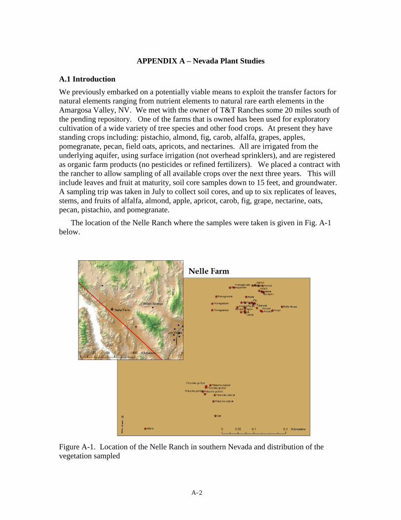
A-2
APPENDIX A –Nevada Plant Studies
A.1 Introduction
We previously embarked on a potentially viable means to exploit the transfer factors fornatural elements ranging from nutrient elements to natural rare earth elements in theAmargosa Valley, NV. We met with the owner of T&T Ranches some 20 miles south ofthe pending repository. One of the farms that is owned has been used for exploratorycultivation of a wide variety of tree species and other food crops. At present they havestanding crops including: pistachio, almond, fig, carob, alfalfa, grapes, apples,pomegranate, pecan, field oats, apricots, and nectarines. All are irrigated from theunderlying aquifer, using surface irrigation (not overhead sprinklers), and are registeredas organic farm products (no pesticides or refined fertilizers). We placed a contract withthe rancher to allow sampling of all available crops over the next three years. This willinclude leaves and fruit at maturity, soil core samples down to 15 feet, and groundwater.A sampling trip was taken in July to collect soil cores, and up to six replicates of leaves,stems, and fruits of alfalfa, almond, apple, apricot, carob, fig, grape, nectarine, oats,pecan, pistachio, and pomegranate.
The location of the Nelle Ranch where the samples were taken is given in Fig. A-1below.
Figure A-1. Location of the Nelle Ranch in southern Nevada and distribution of thevegetation sampled

A-3
A.2 Materials and Methods
The samples were collected July of 2004 at the Nelle farm, placed in paper bags,and shipped overnight to the Pacific Northwest National Laboratory. They were thenunpacked, a fresh weight taken, the samples transferred to tared glass jars, and dried at80°C for 72- to 96-h. Dry weights were then taken and the samples stored at roomtemperature in the closed jars.
The dried samples were then ground with a Wiley Mill (Sargent Welch, Inc.Philadelphia, PA) to a 20 mesh size. The samples were again stored at room temperature.Selected samples (10-g aliquots) have been sent to Huffman Labs, Inc. (Golden,Colorado) for wet digestion and ICP analysis. These are given in Table A-1.
Table A-1. Ten grams of each of the following dried and ground (20 mesh) plant tissuesent to Huffman Laboratories. Golden, CO, for analysis.
GPS Crop Variety TreeID SampleID Segment Code
74 Alfalfa 4 Stem&Leaf AFL-AFS58 Almond 3 3 Leaf ALL58 Almond 3 3 Fruit ALF
55 Apple Goldendelicious 1 1 Leaf AP1L
55 Apple Goldendelicious 1 1 Fruit AP1F
38 Apricot 2,3,4,5 3 Fruit ARF44 Apricot 4 Leaf ARL64 Carob 1 2 Leaf CRL64 Carob 1 2 Fruit CRF53 Fig 4 5 Leaf FIL53 Fig 4 5 Fruit FIF75 Grape 1 1 Leaf GR1L75 Grape 1 1 Fruit GR1F73 Oat Feed 2 All FOL-FOS
67 Pistachio-grafted Grafted 2 3 Leaf GPL
67 Pistachio-grafted Grafted 2 3 Fruit GPF
71 Pistachio-natural Natural 2 3 Leaf NPL
71 Pistachio-natural Natural 2 3 Fruit NPF
39 Pomegranate 1 1 Leaf POL39 Pomegranate 1 1 Fruit POF
Arrangements are being made with the Radiation Center at Oregon StateUniversity to have the bulk of these samples analyzed for a range of constituents using

A-4
neutron activation analysis (NAA). With the NAA technique, very small samples (lessthan 1 gram each) of the plant tissues are irradiated, and the constituents maderadioactive. Neutron activation analysis is a non-destructive, highly precise and accurateanalytical technique capable of determining up to 48 elements in almost all types ofsample matrices. The NAA procedure involves irradiating the samples and appropriatestandard reference materials with neutrons in the Oregon State reactor to produceunstable radioactive nuclides. Many of these radionuclides emit gamma-rays withcharacteristic energies that can be measured utilizing high-resolution semiconductordetectors. The rate that the gamma-rays are emitted from an element in the sample isdirectly proportional to its concentration. Samples as small as 1mg can be quantitativelymeasured by NAA. Detection limits are in the parts per million to parts per billion rangedepending on the element and sample matrix. A new professor at Oregon State hasrecently installed an automated system for performing the sample counting. This shouldallow analysis for a suite of constituents within the next half year.
A.2 Results
The following plants were sampled as shown in Figures A-2 to A-4 and Table A-2.
Fig. A-2. Plants sampled.
Alfalfa
Almond
Field Oat
Apricot

A-5
Fig A-3. Sampled Plants
Carob Nectarine
Natural PistachioGrafted Pistachio

A-6
Fig. A-4. Plants sampled.
Pecan Pomegranate
Fig

A-7
Table A-2. Summary of samples and final dry weights.
GPS Crop Variety TreeID SampleID Segment Code Jar Wt.
(g)Dry Wt.
(g)
TotalSample Wt
(g)74 Alfalfa Feed 1 Stem&Leaf AFL-AFS 232.70 287.69 54.9974 Alfalfa 2 Stem&Leaf AFL-AFS 232.10 281.23 49.1374 Alfalfa 3 Stem&Leaf AFL-AFS 232.85 287.38 54.5374 Alfalfa 4 Stem&Leaf AFL-AFS 231.85 298.89 67.0474 Alfalfa 5 Stem&Leaf AFL-AFS 232.46 292.46 60.0074 Alfalfa 6 Stem&Leaf AFL-AFS 232.25 287.66 55.4174 Alfalfa 7 Stem&Leaf AFL-AFS 192.34 241.11 48.7774 Alfalfa 8 Stem&Leaf AFL-AFS 232.00 277.25 45.2557 Almond 2 2 Leaf ALL 120.49 132.48 11.9957 Almond 2 2 Stem ALS 120.47 150.53 30.0657 Almond 2 2 Fruit ALF 231.64 267.61 35.9758 Almond 3 3 Leaf ALL 120.40 134.74 14.3458 Almond 3 3 Stem ALS 121.53 138.20 16.6758 Almond 3 3 Fruit ALF 233.08 246.40 13.3259 Almond 4 4 Leaf ALL 170.63 178.67 8.0459 Almond 4 4 Stem ALS 121.05 142.26 21.2159 Almond 4 4 Fruit ALF 141.55 171.52 29.9760 Almond 5 5 Leaf ALL 166.06 185.60 19.5460 Almond 5 5 Stem ALS 121.16 158.30 37.1460 Almond 5 5 Fruit ALF 232.79 255.49 22.7061 Almond 6 6 Leaf ALL 172.31 184.30 11.9961 Almond 6 6 Stem ALS 120.45 144.82 24.3761 Almond 6 6 Fruit ALF 233.16 260.78 27.6262 Almond 1 1 Leaf ALL 172.00 183.27 11.2762 Almond 1 1 Stem ALS 121.62 149.19 27.5762 Almond 1 1 Fruit ALF 231.81 255.70 23.89
55 Apple Goldendelicious 1 1 Leaf AP1L 165.88 179.38 13.50
55 Apple Goldendelicious 1 1 Stem AP1S 141.16 174.34 33.18
55 Apple Goldendelicious 1 1 Fruit AP1F 191.33 245.67 54.34
55 Apple Goldendelicious 1 2 Leaf AP1L 165.56 187.58 22.02
55 Apple Goldendelicious 1 2 Stem AP1S 141.16 154.34 13.18
55 Apple Goldendelicious 1 2 Fruit AP1F 192.21 263.83 71.62
63 Apple 2 1 Leaf AP2L 172.17 179.10 6.9363 Apple 2 1 Stem AP2S 142.12 160.34 18.2263 Apple 2 1 Fruit AP2F 142.07 149.68 7.6163 Apple 2 2 Leaf AP2L 121.22 127.65 6.4363 Apple 2 2 Stem AP2S 121.59 139.14 17.5563 Apple 2 2 Fruit AP2F 232.80 265.30 32.50

A-8
38 Apricot 5 1 Leaf ARL 172.45 187.27 14.8238 Apricot 5 1 Stem ARS 232.76 240.79 8.0338 Apricot 5 2 Leaf ARL 171.65 179.08 7.4338 Apricot 5 2 Stem ARS 142.27 151.15 8.8838 Apricot 5 3 Leaf ARL 172.78 181.90 9.1238 Apricot 5 3 Stem ARS 141.78 147.44 5.6638 Apricot 2,3,4,5 3 Fruit ARF 192.51 250.89 58.3844 Apricot 4 Leaf ARL 172.99 188.92 15.9344 Apricot 4 Stem ARS 233.03 261.63 28.60
44 Apricot 4 Fruit ARFTotaledw/ 2,3,
4,545 Apricot 5 Leaf ARL 173.10 194.47 21.3745 Apricot 5 Stem ARS 232.96 253.85 20.89
45 Apricot 5 Fruit ARFTotaledw/ 2,3,
4,546 Apricot 6 Leaf ARL 172.95 197.57 24.6246 Apricot 6 Stem ARS 141.39 159.59 18.20
46 Apricot 6 Fruit ARFTotaledw/ 2,3,
4,564 Carob 1 1 Leaf CRL 165.47 176.30 10.8364 Carob 1 1 Stem CRS 121.76 156.82 35.0664 Carob 1 1 Fruit CRF 231.98 266.71 34.7364 Carob 1 2 Leaf CRL 171.90 188.99 17.0964 Carob 1 2 Stem CRS 121.97 148.85 26.8864 Carob 1 2 Fruit CRF 232.14 254.36 22.2264 Carob 1 3 Leaf CRL 172.16 195.07 22.9164 Carob 1 3 Stem CRS 121.78 160.40 38.6264 Carob 1 3 Fruit CRF 232.81 263.30 30.4965 Carob 2 4 Leaf CRL 120.98 137.95 16.9765 Carob 2 4 Stem CRS 120.59 154.03 33.4465 Carob 2 4 Fruit CRF 141.62 189.46 47.8465 Carob 2 5 Leaf CRL 122.02 139.42 17.4065 Carob 2 5 Stem CRS 121.74 160.95 39.2165 Carob 2 5 Fruit CRF 232.49 281.17 48.6865 Carob 2 6 Leaf CRL 0.0065 Carob 2 6 Stem CRS 121.85 162.46 40.6165 Carob 2 6 Fruit CRF 232.57 284.93 52.3650 Fig 1 1 Leaf FIL 192.83 206.54 13.7150 Fig 1 1 Stem FIS 121.34 139.83 18.4950 Fig 1 1 Fruit FIF 219.72 227.23 7.5150 Fig 1 2 Leaf FIL 165.40 177.13 11.7350 Fig 1 2 Stem FIS 232.13 242.79 10.6650 Fig 1 2 Fruit FIF 218.73 227.48 8.7551 Fig 2 3 Leaf FIL 170.38 181.41 11.0351 Fig 2 3 Stem FIS 232.88 253.36 20.4851 Fig 2 3 Fruit FIF 219.46 227.51 8.05

A-9
52 Fig 3 4 Leaf FIL 192.80 201.81 9.0152 Fig 3 4 Stem FIS 141.13 157.72 16.5952 Fig 3 4 Fruit FIF 219.39 240.29 20.9053 Fig 4 5 Leaf FIL 191.48 209.00 17.5253 Fig 4 5 Stem FIS 121.32 145.88 24.5653 Fig 4 5 Fruit FIF 219.75 235.73 15.9854 Fig 5 6 Leaf FIL 166.33 177.76 11.4354 Fig 5 6 Stem FIS 121.39 135.75 14.3654 Fig 5 6 Fruit FIF 219.53 244.14 24.6175 Grape 1 1 Leaf GR1L 192.94 209.75 16.8175 Grape 1 1 Stem GR1S 191.99 196.80 4.8175 Grape 1 1 Fruit GR1F 191.98 200.18 8.2075 Grape 1 2 Leaf GR1L 191.79 206.11 14.3275 Grape 1 2 Stem GR1S 0.0075 Grape 1 2 Fruit GR1F 121.56 129.95 8.3975 Grape 2 3 Leaf GR2L 166.93 176.39 9.4675 Grape 2 3 Stem GR2S 192.71 198.99 6.2875 Grape 2 3 Fruit GR2F 191.71 216.52 24.8175 Grape 2 4 Leaf GR2L 192.59 207.21 14.6275 Grape 2 4 Stem GR2S 192.45 194.72 2.2775 Grape 2 4 Fruit GR2F 0.0047 Nectarine 1 1 Leaf NCL 192.38 201.96 9.5847 Nectarine 1 1 Stem NCS 121.22 137.25 16.0347 Nectarine 1 1 Fruit NCF 0.0048 Nectarine 2 2 Leaf NCL 166.80 177.81 11.0148 Nectarine 2 2 Stem NCS 141.06 168.23 27.1748 Nectarine 2 2 Fruit NCF 0.0049 Nectarine 3 3 Leaf NCL 165.50 177.23 11.7349 Nectarine 3 3 Stem NCS 121.88 153.33 31.4549 Nectarine 3 3 Fruit NCF 141.95 208.42 66.4773 Oat Feed 1 All FOL-FOS 231.84 354.22 122.3873 Oat Feed 2 All FOL-FOS 232.80 306.62 73.8273 Oat Feed 3 All FOL-FOS 232.16 289.56 57.4073 Oat Feed 4 All FOL-FOS 232.70 296.61 63.9173 Oat Feed 5 All FOL-FOS 232.86 288.27 55.4173 Oat Feed 6 All FOL-FOS 232.99 327.22 94.2373 Oat Feed 7 All FOL-FOS 231.87 283.16 51.2973 Oat Feed 8 All FOL-FOS 231.63 295.48 63.85
56 Pecan-UNKNOWN 1 1 Leaf PCL 122.10 132.22 10.12
56 Pecan 1 1 Stem PCS 121.24 134.80 13.5656 Pecan 1 1 Fruit PCF 142.16 163.38 21.22
66 Pistachio-grafted Grafted 1 1 Leaf GPL 121.65 135.62 13.97
66 Pistachio-grafted Grafted 1 1 Stem GPS 121.81 145.64 23.83
66 Pistachio-grafted Grafted 1 1 Fruit GPF 232.87 280.02 47.15
66 Pistachio-grafted Grafted 1 2 Leaf GPL 122.02 132.62 10.60
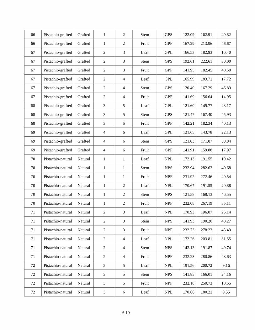
A-10
66 Pistachio-grafted Grafted 1 2 Stem GPS 122.09 162.91 40.82
66 Pistachio-grafted Grafted 1 2 Fruit GPF 167.29 213.96 46.67
67 Pistachio-grafted Grafted 2 3 Leaf GPL 166.53 182.93 16.40
67 Pistachio-grafted Grafted 2 3 Stem GPS 192.61 222.61 30.00
67 Pistachio-grafted Grafted 2 3 Fruit GPF 141.95 182.45 40.50
67 Pistachio-grafted Grafted 2 4 Leaf GPL 165.99 183.71 17.72
67 Pistachio-grafted Grafted 2 4 Stem GPS 120.40 167.29 46.89
67 Pistachio-grafted Grafted 2 4 Fruit GPF 141.69 156.64 14.95
68 Pistachio-grafted Grafted 3 5 Leaf GPL 121.60 149.77 28.17
68 Pistachio-grafted Grafted 3 5 Stem GPS 121.47 167.40 45.93
68 Pistachio-grafted Grafted 3 5 Fruit GPF 142.21 182.34 40.13
69 Pistachio-grafted Grafted 4 6 Leaf GPL 121.65 143.78 22.13
69 Pistachio-grafted Grafted 4 6 Stem GPS 121.03 171.87 50.84
69 Pistachio-grafted Grafted 4 6 Fruit GPF 141.91 159.88 17.97
70 Pistachio-natural Natural 1 1 Leaf NPL 172.13 191.55 19.42
70 Pistachio-natural Natural 1 1 Stem NPS 232.94 282.62 49.68
70 Pistachio-natural Natural 1 1 Fruit NPF 231.92 272.46 40.54
70 Pistachio-natural Natural 1 2 Leaf NPL 170.67 191.55 20.88
70 Pistachio-natural Natural 1 2 Stem NPS 121.58 168.13 46.55
70 Pistachio-natural Natural 1 2 Fruit NPF 232.08 267.19 35.11
71 Pistachio-natural Natural 2 3 Leaf NPL 170.93 196.07 25.14
71 Pistachio-natural Natural 2 3 Stem NPS 141.93 190.20 48.27
71 Pistachio-natural Natural 2 3 Fruit NPF 232.73 278.22 45.49
71 Pistachio-natural Natural 2 4 Leaf NPL 172.26 203.81 31.55
71 Pistachio-natural Natural 2 4 Stem NPS 142.13 191.87 49.74
71 Pistachio-natural Natural 2 4 Fruit NPF 232.23 280.86 48.63
72 Pistachio-natural Natural 3 5 Leaf NPL 191.56 200.72 9.16
72 Pistachio-natural Natural 3 5 Stem NPS 141.85 166.01 24.16
72 Pistachio-natural Natural 3 5 Fruit NPF 232.18 250.73 18.55
72 Pistachio-natural Natural 3 6 Leaf NPL 170.66 180.21 9.55

A-11
72 Pistachio-natural Natural 3 6 Stem NPS 120.87 154.17 33.30
72 Pistachio-natural Natural 3 6 Fruit NPF 232.76 282.80 50.04
39 Pomegranate 1 1 Leaf POL 192.25 205.46 13.2139 Pomegranate 1 1 Stem POS 141.12 150.93 9.8139 Pomegranate 1 1 Fruit POF 192.66 294.59 101.9340 Pomegranate 2 2 Leaf POL 171.67 181.69 10.0240 Pomegranate 2 2 Stem POS 122.12 133.11 10.9940 Pomegranate 2 2 Fruit POF 218.59 306.87 88.2841 Pomegranate 3 3 Leaf POL 171.88 179.97 8.0941 Pomegranate 3 3 Stem POS 121.69 139.67 17.9841 Pomegranate 3 3 Fruit POF 232.89 349.07 116.1842 Pomegranate 4 4 Leaf POL 171.77 179.15 7.3842 Pomegranate 4 4 Stem POS 121.51 137.59 16.0842 Pomegranate 4 4 Fruit POF 191.66 246.84 55.1843 Pomegranate 5 5 Leaf POL 191.66 201.04 9.3843 Pomegranate 5 5 Stem POS 122.09 128.39 6.3043 Pomegranate 5 5 Fruit POF 231.94 364.86 132.9243 Pomegranate 5 6 Leaf POL 171.69 178.64 6.9543 Pomegranate 5 6 Stem POS 121.79 134.27 12.4843 Pomegranate 5 6 Fruit POF 232.88 333.31 100.43
Carob 3 6 Leaf CRL 120.33 133.11 12.78Grape 1 1 Fruit GRF 232.05 241.11 9.06Grape 2 2 Fruit GRF 232.35 245.07 12.72
Nectarine 1 4 Leaf NCL 121.47 138.99 17.52Nectarine 3 6 leaf NCL 121.62 135.50 13.88Nectarine 3 leaf NCL 122.15 140.53 18.38Nectarine 3 Stem NCL 120.83 129.81 8.98Nectarine 1 4 Stems NCS 141.03 172.17 31.14Nectarine 3 5 Stems NCS 232.20 261.29 29.09Nectarine 3 6 Stem NCS 121.74 147.11 25.37
Apricot- fruitcollected from
groundFruit ARF 192.27 316.12 123.85

B- 1
Appendix BIAEA Critical analysis : Arguments for revising the IAEA TRS No. 364

B- 2
IAEA/EMRAS
Revision of the IAEA Technical Reports Series No. 364 : Handbook of parametervalues for the prediction of radionuclide transfer in temperate environments
Critical analysis : Arguments for revising the IAEA TRS No. 364
Pascal Santucci, Gabi Voigt, DRAFT, 4th November 2004comments included : Shigeo Uchida, Sylvie Roussel-Debet
1. Introduction
Most of the safety, performance, or radiological impact assessments concerning either actual orpotential releases, when they comprise biosphere calculations, use parameters such as transfer oraccumulation factors requiring their associated values. One international example is the IAEASRS No. 19 (2001) on the assessment of routine releases. If future assessment purposes arecurrently considered, such as those linked to overall environmental impact assessments (Hunter,2001), most of the current biosphere models still need such parameters and associated values.
In the literature, as said by Whicker et al. (1999), overall syntheses are not very numerous(e.g. the well known Coughtrey, Jackson and Thorne, 1985). One important document is widelyused by the scientific community : the IAEA Technical Reports Series No. 364, "Handbook ofparameter values for the prediction of radionuclide transfer in temperate environments",published in collaboration with the International Union of Radioecologists (IUR) in 1994. Itscontents reflected radioecological results up to 1992. TRS 364 is widely used as a major source ofinformation, because it addresses numerous environmental transfer parameters and radionuclides.It is therefore quoted in numerous impact assessments, even if amended or completed by thescientific community (radiation protection, radioecology). Moreover, many radiation protectionmodels need to predict transfer of a large number of radionuclides. This requires information ontransfer of many less mobile radionuclides, which do not usually comprise an importantcomponent of discharges or dose. Such information is often sparse and difficult to collate. TRS364 provides an important source of such information, and is one of the key cited sources formany models. It is thus essential that such information is kept up-to-date and that any relevantrecent literature is included, especially considering the paucity of existing data sources.
Since 1992, new data have also been produced, such as post-Chernobyl information (Shaw,2001), and new experimental results (e.g. lysimeter studies), potentially completing the existingdata and syntheses, which are now more than 10 years old. A number of high quality criticalreviews have been produced in recent years for some of the transfer parameter values which meritconsideration. International programmes have also been devoted to the construction andvalidation of radioecological models : BIOMOVS, IAEA/VAMP, IAEA/BIOMASS, EuropeanFrameworks, etc. It is then assumed that there is sufficient new information available to warrantreconsideration of a significant proportion of the values given in TRS 364.
As a consequence, there are arguments for updating TRS 364 and extending it, in terms ofcompartments, processes and radionuclides, and even for improving its current contents, becausea critical analysis can highlight some weaknesses. This explains why the IAEA decided in 2003

B- 3
to include the revision of TRS 364, as a topic of the EMRAS programme, "Environmentalmodelling for radiation safety".
2. Justification for the performance of an updated synthesis at an international level
Behind the necessity to take into account progress of science and knowledge, one question is toknow to what extent it is useful or necessary to sustain an international work on that field, ratherthan letting individuals manage the existing information.
During the IAEA/BIOMASS programme, a group was devoted to the issue regarding dataselection for biosphere assessment models. It showed that even if biosphere parameters cannot beconsidered as "constant" as the ICRP dose coefficients, they can be tabulated : as default valueswhen well characterised : this could be the case for IUR soil-to-plant transfer factors, according tobroad crop groups ; as example values or representative values, directly used if the parameter isnot much important in the assessment ; as a starting point if the parameter appears critical (linkwith sensitivity and uncertainty analyses).
Compilation and tabulation of data is then useful, but if the people in charge of such a workhave limited expertise (scope) and little resources, there is a risk of introducing biases during theprocess of data selection (see discussion about expert judgment, e.g. Thorne&Williams, 1992) :
- Representativeness of data, e.g. : individuals are insensitive to sample size : the sameweight, or level of confidence, can be attributed to parameter values for which there are muchor little data (issue when the assessment addresses a broad spectrum of radionuclides) ;individuals are over-sensitive to information, even when information is not related to data :see discussions about site-specific data.
- Availability of data, e.g. : individuals favour the easily available and understandableinformation : it is a question of review management, but also of institutional culture ;individuals can misinterpret the co-occurrence of naturally associated characteristics : theinfluence of potential co-factors could then be assumed rather than tested.
- Anchoring, e.g. : individuals have difficulties to depart from initial values they know, evenif the assessment context requires it ; individuals have the tendency to underestimate therange of variation of a parameter.
From these arguments, it follows that : review and syntheses performed by individuals orsmall groups will generally be limited in scope (few compartments and processes) for a givenassessment context. The recourse to structured elicitation exercises appear interesting, but it isresource consuming and past experience has shown that it is difficult to systematically implementthem (US/NRC&EU on COSYMA, BIOMASS on data selection) ; according to someparticipants, their intrinsic value may even look doubtful ... An intermediate way is to try to buildsyntheses and databases at an international level : access to a large audience with variousbackgrounds and levels of expertise, optimisation of resources by the sharing of the overall effort(e.g. by ecological field) and the already existing material (reviews, bibliographic material,databases).

B- 4
3. General features of the revision of IAEA TRS No. 364
Due to the large audience and use of TRS 364, there is a need to keep such a document asrelevant, accurate and consistent as possible : relevant first, because the purpose is to covervarious assessment contexts such as routine releases and accidental conditions, atmospheric andliquid releases, etc. It should be accurate because mistakes should be corrected and avoided, up-to-date science should be incorporated (this could be difficult when data is scarce, as is the casefor less mobile radionuclides). And last, it should be consistent : consistency between tablesshould be ensured, especially with regards to the list of radionuclides considered, all the moresince integrated assessments require it.
An assessment of the quality of data obtained is of paramount importance to assure that thesuggested best estimates of the environmental parameters can be used in generic predictivemodels. In an ideal world, a critical evaluation of data would include a statistical analysis of thedata. However, because of the availability of resources, this was not attempted in TRS 364, and itmay be difficult to carry it out in a revision.
In practice, the expected values and ranges given in TRS 364 are based on a variety ofdifferent approaches which are not clearly specified for each value. They comprise statisticalanalysis, expert judgement or sometimes only a single experiment. For some of the tables (e.g.animal transfers) the approach has been specified for each value ; it is recommended to extendthis approach to all other tables as far as possible.
Uncertainty should be mostly addressed by giving ranges of variation ; in some casesprobability density functions could be built through the performance of statistical analyses ofdatabases (e.g. on some Kds and soil-to-plant transfer factors). The question should be raisedabout the extrapolation of their statistical results to other categories (e.g. confidence intervalsextrapolated from one radionuclide to another). When data is scarce or missing, a discussionshould be held concerning the use of chemical analogues as a way of completing the tables.Variability could be reduced by revising classification systems (e.g. crop groups) and introducingco-factors (e.g. with Kds, soil-to-plant TFs).
Steady state models are routinely used for dose assessment, for screening purposes andoperational releases. Information in the TRS 364 is directly relevant for such models, when timedependency in transfers is neglected. Many dynamic models are intended for dose assessment inemergency situations. For such models, often both empirical (using classification of systems) andsemi-mechanistic approaches are used. The availability and applicability of improved dynamicmodels based largely on mechanistic information is limited. In general, such models have onlybeen developed for a small number of radionuclides (notably caesium and strontium), inparticular types of system, such as caesium behaviour in soils, forests or freshwaters ormetabolically based models of animals. Such models have the additional advantage of being ableto include the effect of countermeasures in a mechanistic way and complement other moregeneralised models used for radiation protection purposes. It is therefore important to considerwhether the continued use of empirical transfer values is always justified and appropriate.
For an accurate mathematical description of dynamic processes a multi-compartment model,in which the material fluxes are described by mechanism-based rate equations, is essential. Suchdynamic models apply to cycling of radionuclides in ecosystems, retention and accumulation,migration and leaching. It is recognised that complex dynamic models, all the more because theyoften lack consensus and large validation, are outside of the scope of a revised TRS 364. Anexception is made for dynamic one-compartment models in which processes can be modelled by

B- 5
a half-life concept. The dynamics of some of these processes are so important, that neglectingthem would be a serious shortcoming of the new TRS. A consideration of changes with time interrestrial and aquatic systems, expressed as ecological half-lives in different food products andreflecting processes involved in the long-term transfer from soil to vegetation, provides animportant improvement for modelling.
Nomenclature should be tested against official documents such as ICRU 65 (2001)"Quantities, Units and Terms in Radioecology" : it contains a list of units and quantitiesfrequently used in the field of radioecology, and tries to harmonise these units derived fromvarying different disciplines such as ecology, chemistry, medicine or physics.
4. Analysis and completion of the existing TRS 364
4.1. Methodology
Section by section (based on ecological domains), the methodology for reviewing the currentsynthesis is the following : list the processes of interest ; review the modelling aspects, in terms ofcompartments and processes, minimum model representation, alternative modelling, potential co-factors ; analyse the radionuclides currently taken into account ; consider the classificationsystems ; highlight weaknesses and mistakes ; and check the availability of new data for selectionand inclusion in a new TRS.
When rewritten, the sections will be articulated according to a main text devoted toexplaining the main processes involved, with the usual associated parameters, co-factorsinfluencing some processes or the determination of parameters values, and key equations used fordescribing and assessing the transfers. The IAEA SRS 19 could be a basic reference for simplemodelling. Besides, tables of transfer coefficients will be displayed, with values depending onspecies (or groups of species), environmental conditions, co-factors, etc. The references used willbe quoted.
4.2. Agricultural systems - Foliar interception, retention and translocation
Foliar interception is a prominent process after initial release from a nuclear facility. The sectionis not clear enough and not self-sufficient for building the intended model structure. It showsstrong link with plant characteristics, at least because the plant stage of development is a veryimportant factor. For contamination of surfaces, three deposition pathways are considered : directdry or wet deposition and resuspension processes. With regard to the latter, only the soil adhesionto vegetation is considered since it may affect the ingestion dose.
The interception values for dry deposition refer to experimental work mostly performed in theearly nineteen seventies. Values relating to wet deposition refer mainly to two referencespublished in 1965 and 1977. Meanwhile, much more data has become available which needs tobe included, such as experimental and post Chernobyl studies. Also information on theseasonality of intercepted fractions relating to the biomass of different plant species could begreatly improved (in TRS 364 only one reference is given). Instead of providing individualexperimental results, a critical compilation of values showing the dependence of interceptedfractions on the precipitation intensity, time lack, season and plant species should be tabulated. Ithas also been deemed useful to introduce deposition velocities. Since there is a requirementarising from the waste assessment field, irrigation processes, considered as a particular case of thewet deposition, should also be introduced.

B- 6
Under accidental conditions, parameter values should not be averaged over the year. Withsuch a context, the physico-chemical features of the source-term may be of importance(granularity, solubility). The amount of rainfall should also be specified. The European RODOSprogramme could be an important source of information.
In TRS 364, the processes of foliar absorption, translocation and retention need to be clearlydistinguished. In TRS 364, a collation of different translocation coefficients for crops with timedependencies before harvest are given, however conclusions or recommendations on whichvalues to use are not provided. The aim should be to derive generic parameter values from areview of revised data compilation. In addition, the conclusions and recommendations in IAEA/TECDOC 857 (1996) should also be considered.
New data can be added on the transfer to fruit. Inclusion of time dependency in trees andunderstory vegetation (berries) and retention in the canopy information on interception andtranslocation might be useful as their features are different from the other crop groups.
4.3. Agricultural systems - Soil retention and migration : Kds
The current classifications of soil systems used in TRS364 are rather simplistic and limited toonly four categories: sand, loam, clay and peat ; they are somewhat inadequate to account for thesoil parameters that govern the behaviours of different RN. The values were based on a relativelylow number of experiments for a limited number of soils within each category. In recent years thenumber of data for each category has greatly increased, and analysis of the data distribution hasshown a high variability and high degree of overlap. Revised classification systems are currentlydeveloped which are based on mechanistic information including consideration of parametervalues such as pH, soil nutrient status, % clay, exchangeable K and Ca in soil, moisture content ofsoil, organic matter content and the time that a radionuclide is present in a soil. Numerousmultiregression analyses have been developed and give reasonable predictions on a local scalebut have not been proven on a world-wide scale. At least for some radionuclides (e.g. Cs, Sr, U,Tc) a semi mechanistic approach should be used.
4.4. Agricultural systems - Uptake from soil to plant
At the time that TRS 364 was prepared, the IUR had already introduced “crop groups” as cereals, green vegetables, root crops, etc. It was, however, not yet then possible to use these crop groupsto provide expected uptake parameters, so separate transfer values were provided for wheat,barley, rye, etc. These crop groups should now be introduced.
Currently, data given on soil-to-plant transfer factors given in TRS 364 generally uses threeapproaches :
For Cs and Sr, separate values are given for different soil categories (sand, loam, clay andpeat) with a pH constraint. In recent years, the number of data for Cs and Sr has greatly increased,and analysis of the data distribution has shown a high variability and high degree of overlap.Revised classification systems are currently being developed which are based on mechanisticinformation including consideration of parameter values of co-factors, such as pH, soil nutrientstatus, % clay, exchangeable K and Ca in soil, moisture content of soil, organic matter contentand the time that a radionuclide is present in a soil, in consistency with those adopted for Kds.

B- 7
For Pu, Am and many other radionuclides, soil type is not considered. The data have largelybeen collated between 1980 and 1990. For some of them, e.g. Pu, Am, Co, Mn, Tc, Zn, new dataare available. For others it is doubtful that sufficient values for updating tables are available.
Less frequently studied radionuclides are generally based on much older literature. There areprobably few data available.
Both for the second and third group it is probably worthwhile to consider the uptake data ofstable elements. In particular, heavy metals have received considerable recent attention.
4.5. Agricultural systems - Transfer from feed to animal products
This section could be improved by a review of recent literature even if new data are more difficultto find than for plants. For many of the radionuclides, the tabulated data are based on acompilation originating from databases more than 20 years old. The intake rates of feedstuff byanimals are based on European conditions only and should be supplemented by data for otherareas of the world. Some FAO activities and results could be of use.
For ingestion doses the application of equilibrium transfer coefficients for animal products isinappropriate for radionuclides with long biological half-lives. Therefore, in TRS 364 sometransfer coefficients were modified to account for a known lack of non-equilibrium. Thisapproach needs to be extended, possibly by providing half-life information, and evaluated.Furthermore for strontium, iodine and caesium information on biological half-lives is availableand can be compiled.
A statistical analysis of the data is not possible for TRS 364 because many of the values camefrom reviews using extensive data and individual data sets which were not available.Supplementation of recent data with these reviews was attempted, but was only possible usingexpert judgement. For some selected radionuclides a statistical analysis could be performed sincesufficient data and data sets are available. However this would be extremely time consuming andis unrealistic. It is therefore recommended to use recently published reviews where statisticalanalysis have been attempted.
In the last decade detailed and improved information on the influence of stable analogues forcaesium, strontium and iodine has become available and should be considered for inclusion inrevision of TRS 364.
4.6. Freshwater systems
This chapter should be rewritten and enhanced in terms of compartments and processes included,and environmental conditions, in consistency with the IAEA SRS 19 ; in particular, bottomsediments and water particles should be distinguished, as well as trophic levels for fish.
Concerning partition coefficient suspended matter/water : The adsorption and desorptionprocesses of radionuclides by suspended matter strongly influences the behaviour of radioactivesubstances in freshwater systems. Consequently, considerable research has been carried out onthese processes. The most common and simple approach for modelling the adsorption/ desorption

B- 8
processes at equilibrium is based on the partition coefficient Kd. The correlation between thepartition coefficient and the chemical characteristics of the water body should be described. Avariety of researchers have demonstrated that non reversible adsorption processes are ofimportance for some radionuclides, notably caesium. A table of non reversible fraction rates forcaesium in different freshwater ecosystems should be included.
Concerning other relevant migration processes and parameters : Among the various processesoccurring in water bodies the thermal stratification phenomena of deep lake water may stronglyinfluence the concentration of any floating material in the water column. Stratification and de-stratification have a marked seasonal behaviour which can result, even for steady state releases, insignificant seasonal variation in contamination levels in water and fish. During the stratificationperiod, the diffusion of dissolved radionuclides in the upper layer of lake water (epilimnion) tothe bottom water layer (hypolimnion) is prevented by the presence of an intermediate layer(thermocline) that shows a marked temperature gradient. To be able to model the above process,effective diffusion coefficients are needed. Furthermore, more data are required for parameters ofmigration from water column to bottom sediments possibly including migration velocity.
In TRS 364, the table concerning fish is based on a large database for a wide range ofelements. However, the method of selection for the expected values is not specified and appearsto be inconsistent. However, data are quite comprehensive and might be supplemented by a fewrecent literature reviews on concentration factors for the edible portion of fish in freshwaterenvironments.
4.7. Semi-natural ecosystems : forests
It is important to include semi-natural ecosystems for caesium because the range of productsharvested differs greatly from other ecosystems and the rate of transfer to food products is oftenmuch higher than for other ecosystems. Furthermore, the ecological half-lives of caesium in manyproducts harvested from these ecosystems is much longer than in agricultural systems. For somepopulations, consumption of semi-natural products is common, for others it is confined to certainspecial groups. For both cases, such consumption can form a major proportion of ingestion dosein the mid-long term after deposition.
The section on semi-natural ecosystems in TRS 364 was largely based on simple aggregatedtransfer coefficients, since the inherent variability and complexity of such systems makepredictions using other approaches difficult. Recently, some dynamic models have beendeveloped which allow the estimation of transfer to certain forest products, but the number ofproducts considered is limited. It is therefore recommended that the same parameter should beused in the revision to be able to include as wide a range of products as possible. The extension ofthe radionuclide spectrum should also be sought. Fortunately, data availability has greatlyincreased since 1992, largely from the considerable focus in both Europe and the CIS on caesiumtransfer to forest products.
Some game species and humans consume large quantities of mushrooms which can take uplarge quantities of Cs. Mushroom consumption can therefore be a dominant pathway for theingestion of caesium. Currently much more data on mushroom transfer have now becomeavailable. For arctic systems significant improvement of TRS 364 is now possible for quantifyingtransfer of caesium to reindeers and its time dependency, based on a review carried out under theArctic Monitoring and Assessment Programme (AMAP).

B- 9
Recent analysis of transfer to macrofungi suggested that it is not statistically valid to giveseparate values for individual mushroom species, as done in TRS 364. Instead, tag values forecological categories could be more appropriate (mycorhizal, saprophitic and parasitic). Reviewsof tag values are now available for many products and it should be possible to acquire or carry outstatistical analysis of data for many products. In addition, improved ecological half-life data areavailable for many products, notably reindeer, moose, roe deer and wild boar, and should now bereported.
Descriptive text on the transfer processes for each food product could be substantiallyimproved and extended. Mushroom species with consistently higher transfer values than the meanfor their ecological category could be identified (e.g. Rozites caparata). In addition, it may bepossible to give some information on the dependency on soil type for a few mushroom species.
4.8. Food processing
There are a lot of tables, but they are particularly useful in a context of accidental management. Itis recommended to simplify them by focusing on the most efficient processes for radioactivityreduction. For instance, one could focus on the processing of dairy products and mushrooms.
5. Extension of TRS 364 in scope, compartments and processes
5.1. Radioelements
At a methodological level, a discussion on chemical analogy should be introduced as a way toovercome the lack of data for some radionuclides, especially if consistency between the tablesshould be reached.
There are so-called "special" radionuclides such as 3H, 14C, maybe even iodine or chlorine. Ifpossible, it is suggested to keep their specificity, provided that data could feed the tables. Specificmodels should be explicited.
5.2. Climate conditions
TRS 364 was limited to temperate climatic zones because, at the time, few data from otherclimatic zones were available. Since 1992, new data on both arctic regions and tropicalenvironments have become available. From this new data it appears that the climate itself seemsto have little direct influence on radioecological transfer parameters, but that nevertheless theimpact of the climate on other important parameters is large. Climate and parent rock materialdetermine, to a large extent, the development of soil type.
In tropical areas, several soil types occur in which radionuclide uptake by crops consistentlydeviate from the expected values given in TRS 364. Under these hot and wet conditions almostall organic material which reaches the soil surface decomposes rapidly; the accumulation of soilorganic matter is therefore minimal, and there is rapid recycling into the vegetation. In temperatezones, the decomposition of organic debris is slower and accumulation of soil organic matter canbe larger than the rate of decomposition resulting in highly organic soils.

B-10
In arctic regions, ammonium, which is formed during decomposition of organic matter, maynot be completely oxidised, leaving it available for competition with radionuclide cations.Ammonium has a five fold higher affinity than potassium for illitic adsorption sites; thisinfluences the fixation of caesium.
Such examples show that if at least fundamental processes are well documented, theirdependence on temperature could be taken into account.
5.3. Asian food-chains
Because agricultural products and food customs in Asian countries are different from those intemperate ones, it is expected that the critical foods differ as well. In European and NorthAmerican countries, livestock products including meat, eggs, and milk make a big contribution,while, in Asian countries, agricultural products including cereals and vegetables are the maincontributors.
It has also been suggested to extend TRS 364 by introducing Asian food chains. Such food-chains refer to several climate conditions, from temperate to tropical. Some crops are grownunder particular conditions, as is the case for flooded rice.
The FAO/IAEA, in cooperation with IUR, has established various programmes which are ofuse for feeding a new TRS : namely, those entitled "Transfer of radionuclides from air, soil, andfreshwater to the foodchain of man in tropical and sub-tropical environments" (1993-1997), and"The Classification of Soil Systems on the Basis of Transfer Factors of Radionuclides from Soilto Reference Plants" (1999-2003).
5.4. Secondary pathways of contamination
Atmospheric resuspension and wash-off should be introduced as new processes because they areprominent secondary pathways of contamination.
Wash-off amounts to roughly less than 1%.y-1 for Cs and Sr : it is not important in terms oflosses (in a short term period), but it is very important for the secondary contamination of rivers.It depends on amount of water, soil cover, slope or profile. Erosion is included in wash-off. Thereis a competition with vertical migration, which is an argument for time-dependency. In recentyears, many attempts have been carried out to develop new approaches which allow modellers topredict radionuclide migration from catchments by using more simple generic models includinghalf-lives and transfer factors. Due to the data available in the international literature followingthe Chernobyl accident, it is possible to produce a limited, but somewhat instructive, list of half-lives and transfer factors mainly for 90Sr and 137Cs. This list could be helpful for generic modelsapplicable to both steady state and dynamic conditions.
Resuspension and soil adhesion are relevant when soil to plant transfer factors are low (slowtransfers). However, soil adhesion should not be taken too seriously due to the interaction withfood processing (washing, peeling, etc.).

B-11
6. Revision of TRS 364 in practice ...(we are waiting for organisation by section)
- The revision of TRS 364 is one of the main activities of the IAEA programme EMRAS(Environmental modelling for radiation safety), 2003-2006(7)
- The overall work plan is the following (per year) :- September 2003, EMRAS plenary : about 20 participants ; agreement on work andmilestones- November 2004, EMRAS plenary : first draft on the critical analysis of TRS 364, synthesison new available data, draft of computerised database- End 2005, EMRAS plenary : final documents on the TRS critical analysis and on dataavailability, draft of TRS concerning already included parameters, draft on newparameters/ processes to be included, draft CD-rom with new data- End 2006, EMRAS plenary : draft of overall new TRS, draft 2 of CD-rom with source data2007 : finalisation of TRS
- Material :- nearly 90% of the TRS 364 references have been recovered (about 200)- about 400 new references of interest have been found (later than 1992), including reviewsand syntheses ; the grey literature should not be discarded if valuable (institutional reports)which is the case with some overall syntheses- some databases : IUR for soil-to-plant transfers, IAEA CRP on tropical systems, EURadFlux multi-compartments too, national databases (NRPB, IRSN) on Kds, soil-to-plantTFs, animals, food processing
- Collaboration with IUR :- TRS 364 was issued in collaboration with IUR- most of the IAEA/EMRAS participants belong to IUR- the well known database on soil-to-plant TFs was managed by IUR ; IUR was a co-sponsorof RadFlux- there are IUR working groups of interest for the revision (radioecology of rice, radioecologyand waste (special radionuclides)), which explains that this revision is also an IUR activity- an official agreement between IAEA and IUR is about to be reached, as a way to benefitalso from the IUR audience
7. Conclusion
The revision of the IAEA TRS No. 364, "Handbook of parameter values for the prediction ofradionuclide transfer in temperate environments", published in collaboration with the IUR, is anambitious effort which is required by the progress of radioecology, expected by numerous users,and made possible by an international collaboration launched through the IAEA/EMRASprogramme.

B-12
Since such an activity demands expertise and resources, all institutions, all experts arewelcome to contribute and participate through the existing channels : IAEA/EMRAS, IUR oreven personal contacts.
8. References
Coughtrey, P.J., Jackson, D., Thorne, M.C., 1985. Radionuclide Distribution and Transport inTerrestrial and Aquatic Ecosystems - A compendium of data. Balkema, A.A. Publishers,Rotterdam, Netherland.
Hunter, G., 2001. Developments in radioecology in the new millennium. Journal ofEnvironmental Radioactivity 56 (2001) 1-6.
IAEA, 1994. Handbook of parameter values for the prediction of radionuclide transfer intemperate environments. IAEA Technical Reports Series No. 364. International Atomic EnergyAgency, Vienna, Austria.
IAEA, 1996. Modelling of radionuclide interception and loss processes in vegetation and oftransfer in semi-natural ecosystems. TECDOC No. 857, Second report of the VAMP TerrestrialWorking Group. International Atomic Energy Agency, Vienna, Austria.
IAEA, 2001. Generic models for use in assessing the impact of discharges of radioactivesubstances to the environment. IAEA Safety Reports Series No. 19. International Atomic EnergyAgency, Vienna, Austria.
ICRU, 2001. Report 65 : Quantities, Units and Terms in Radioecology. Journal of the ICRU,vol. 1, n° 2. International Commission on Radiation Units and Measurements, NuclearTechnology Publishing, Ashford, England.
Shaw, G., 2001. Radioecology–How did we get here and what do we do now ? Journal ofEnvironmental Radioactivity 54 (2001) 305-309.
Thorne M.C., Williams M.R., 1992. A review of expert judgment techniques with reference tonuclear safety. Progress in Nuclear Energy, Vol. 27, No. 2/3, pp. 83-254.
Whicker F.W., Shaw, G., Voigt, G., Holm, E., 1999. Radioactive contamination : state of thescience and its application to predictive models. Environmental Pollution 100 (1999) 133-149.