assessment of the equivalent level of safety requirements ... · assessment of the equivalent level...
TRANSCRIPT

ASSESSMENT OF THE EQUIVALENT LEVEL OF SAFETY
REQUIREMENTS FOR SMALL UNMANNED AERIAL VEHICLES
by
© Jonathan D. Stevenson, B.Eng., M.Eng.
A Doctoral Thesis submitted to the
School of Graduate Studies
In partial fulfillment of the requirements for the degree of
Doctor of Philosophy
Faculty of Engineering and Applied Science
Memorial University of Newfoundland
June 2015
St. John’s Newfoundland and Labrador
ii
ABSTRACT
The research described in this thesis was a concentrated effort to assess the
Equivalent Level of Safety (ELOS) of small Unmanned Aerial Vehicles (UAVs), in terms
of the requirements needed for the small UAV to be considered at least as safe as
equivalent manned aircraft operating in the same airspace. However, the concept of
ELOS is often quoted without any scientific basis, or without proof that manned aircraft
themselves could be considered safe. This is especially true when the recognized
limitations of the see-and-avoid principle is considered, which has led to tragic
consequences over the past several decades. The primary contribution of this research is
an initial attempt to establish quantifiable standards related to the ELOS of small UAVs in
non-segregated airspace. A secondary contribution is the development of an improved
method for automatically testing Detect, Sense and Avoid (DSA) systems through the use
of two UAVs flying a synchronized aerial maneuver algorithm.

iii
ACKNOWLEDGEMENTS
The author was supported financially through the National Sciences and Research
Council of Canada, including the generous granting of a Canadian Graduate Scholarship.
RAVEN flight operations of the Aerosonde UAV would not have been possible without
the financial support from the Atlantic Canada Opportunity Agency and our industrial
partner, Provincial Aerospace Limited (PAL).
The experiments at Argentia and Bell Island were assisted by the enthusiastic
participation and support of the RAVEN team, especially during operations in 2010 and
2013. The night-time light experiment required the enlistment of a number of volunteer
human test subjects, whose valuable contribution to this research is hereby noted.
The author also wishes to thank of his supervisors, Dr. Siu O’Young and Dr. Luc
Rolland, for their unwavering support, encouragement and assistance, especially during
the final stages of this research and the preparation of the thesis.
The support of my family made the sometimes arduous research bearable. My six
month sabbatical in 2013 would not have been possible without my parents’ support
including accommodations. My older brother Christopher deserves special mention for
his assistance in the preparation of the thesis draft copies for submission.
Finally, the care, encouragement and support provided by my partner, Rennie,
including serving as the “cook” for the human subjects during the night-time light
experiment, is greatly appreciated. This project would not have been completed successfully
without her support.

iv
Table of Contents
ABSTRACT ....................................................................................................................... ii
ACKNOWLEDGEMENTS............................................................................................... iii Table of Contents................................................................................................................ iv List of Tables ................................................................................................................... viii List of Figures .................................................................................................................. viii List of Symbols, Nomenclature or Abbreviations ............................................................... x
List of Appendices ............................................................................................................ xiv Chapter 1 Introduction ...................................................................................................... 1
1.1 The Motivation for Unmanned Aerial Vehicles .................................……1
1.1.1 The Original Military Role ................................................................................ 1
1.1.2 Expansion to Non-Military Roles ..................................................................... 3
1.1.3 The Utility of UAVs.......................................................................................... 4
1.1.4 Classification of UAVs ..................................................................................... 6
1.1.5 The Role for Small LALE UAVs...................................................................... 8
1.2 The Challenges and Limitations of UAVs ................................................. 9
1.2.1 Lack of Pilot See and Avoid Capability .......................................................... 10
1.2.2 Inadequate Anti-Collision Technologies......................................................... 10
1.2.3 No Detect, Sense and Avoid System ............................................................... 11
1.2.4 Limited BLOS Situational Awareness ............................................................ 12
1.2.5 Unique Challenges for the Small LALE ......................................................... 14
1.3 Problem statement .................................................................................... 17
1.3.1 Risk Assessment.............................................................................................. 17
1.3.2 Definition of Equivalent Level of Safety ........................................................ 18
1.3.3 Summary of the Detect Sense and Avoid Problem ......................................... 21
1.4 Thesis Outline .......................................................................................... 23
Chapter 2 Assessing the Risks Posed by UAVs ............................................................. 26
2.1 The Requirements for UAV Integration .................................................. 26
2.2 Perceived and Assumed Risks ................................................................. 30
2.2.1 Risk to the Crew .............................................................................................. 30
2.2.2 High Operational Costs ................................................................................... 32
2.2.3 Financial Risk due to Attrition ........................................................................ 32
2.2.4 The Doctrine of Zero-Tolerance ..................................................................... 34
2.2.5 Public Fear of UAVs ....................................................................................... 35

v
2.2.6 Motivation for Improved Reliability ............................................................... 36
2.2.7 The Motivation for UAV Control Enhancement Research ............................. 37
2.3 Physical Risks from UAVs ...................................................................... 38
2.3.1 Ground Impact Risk ........................................................................................ 39
2.3.2 Mid-Air Collision Risk ................................................................................... 41
2.4 Calculating the Estimated Level of Safety ............................................... 44
2.4.1 Ground Impact Estimated Level of Safety ...................................................... 44
2.4.2 Mid-air Collision Risk..................................................................................... 50
2.5 Summary: The Current Level of Safety ................................................... 58
2.5.1 Ground Risk .................................................................................................... 58
2.5.2 Mid-Air Collision Risk ................................................................................... 59
2.5.3 Where the Small UAV Needs to Improve ....................................................... 59
2.5.4 Mitigation Strategies ....................................................................................... 60
Chapter 3 UAV Control and Situational Awareness ...................................................... 62
3.1 Introduction to UAV Control Methods .................................................... 62
3.2 Analysis of UAV Control Methods ......................................................... 66
3.2.1 Summary of the Manual Control Situation ..................................................... 67
3.2.2 First Person versus Third Person View ........................................................... 69
3.2.3 The Problem of Control Delays ...................................................................... 71
3.3 Virtual Reality Pilot Experiments ............................................................ 77
3.3.1 Various Manual Piloting Methods .................................................................. 77
3.3.2 The VR Landing Experiment Design .............................................................. 79
3.3.3 Argentia VR Landing Experiment (2010) ....................................................... 81
3.3.4 Bell Island Landing Experiment (2013) .......................................................... 96
3.3.5 Conclusions from Both VR Experiments ...................................................... 109
3.4 Extended Range Video Links at Beyond Line of Sight ......................... 111
3.5 Synthetic Environments ......................................................................... 115
3.5.1 Visualization using a Flight Simulator .......................................................... 115
3.5.2 Enhancements using Multi-Player Mode ...................................................... 118
3.5.3 Tests of the Synthetic Environment in Clarenville ....................................... 119
3.5.4 Extension of Synthetic Environment for BLOS Control .............................. 121
3.6 Summary: Effect of Enhanced UAV Control Methods on Safety ........ 123
Chapter 4 Enhancements to UAV Visibility ................................................................. 125
vi
4.1 Theoretical Visibility Estimates ............................................................. 125
4.1.1 The Human Factors of Vision ....................................................................... 126
4.1.2 Day-Time Visibility ...................................................................................... 134
4.1.3 Night-Time Visibility .................................................................................... 145
4.2 Experiments with Anti-Collision Lights ................................................ 152
4.2.1 Night-Time VFR Light Experiment .............................................................. 153
4.2.2 Extended Range Observations ...................................................................... 164
4.2.3 Daytime VFR Anti-Collision Light Testing ................................................. 165
4.2.4 Conclusions from Anti-Collision Light Experiments ................................... 166
4.3 An Equivalent UAV Vision Capability ................................................. 167
4.3.1 Visual Acuity ................................................................................................ 167
4.3.2 Field of View and Scanning Ability .............................................................. 167
4.3.3 Better than Human Vision Abilities .............................................................. 168
4.4 Transponder Technologies ..................................................................... 168
4.4.1 Miniature Mode-S Transponders .................................................................. 169
4.4.2 Automatic Dependent Surveillance-Broadcast Transponders ...................... 172
4.5 Air-band Radios ..................................................................................... 173
4.6 Summary: Impact of Visibility Enhancements on Safety ...................... 174
Chapter 5 4D Simulations and Avoidance Maneuvers ................................................. 176
5.1 4D Encounter Simulation Environment ................................................. 176
5.1.1 Historical Background .................................................................................. 177
5.1.2 Simulation Structure...................................................................................... 179
5.1.3 Mathematical Basis of the Aircraft FDM...................................................... 182
5.1.4 4D Encounter Simulations using Multiplayer ............................................... 187
5.2 Development of 4D Encounter Geometries ........................................... 191
5.2.1 Opposing Circuits.......................................................................................... 191
5.2.2 Time-Synchronization Methods .................................................................... 195
5.2.3 The PHI Maneuver ........................................................................................ 198
5.2.4 The PHI Maneuver with Active Guidance .................................................... 200
5.3 Avoidance Maneuvers ........................................................................... 202
5.3.1 Rules of the Air and Right-of-Way ............................................................... 202
5.3.2 Manned Aircraft versus UAVs...................................................................... 205
5.3.3 UAV Avoidance Algorithms......................................................................... 214
vii
5.4 Predicted 4D Simulation Results ........................................................... 221
5.4.1 Base PHI-Maneuvre Results (Passive Aircraft) ................................. 221
5.4.2 Active Interceptions by the Intruder (Target Passive) ....................... 222
5.4.3 Active Avoidance by the Target (Passive Intruder) ........................... 224
5.4.4 Active Intruder and Active Target ..................................................... 225
5.5 Summary ................................................................................................ 226
Chapter 6 Conclusions and Recommendations ............................................................. 228
6.1 The Equivalent Level of Safety of small UAVs .................................... 228
6.2 Proposed Improvements to Safety ......................................................... 229
6.2.1 Improvements to Ground Risk Safety ........................................................... 230
6.2.2 Reduction of Mid-Air Collision Risk ............................................................ 232
6.2.3 Impact of Mitigation Strategies on Ground Impact Safety ........................... 237
6.3 Proposed Minimum DSA Requirements for small UAVs ..................... 239
6.4 Conclusions ............................................................................................ 242
6.5 Recommendations for Future Research ................................................. 246
References ....................................................................................................................... 248 Appendix A – Project RAVEN ....................................................................................... 267
Appendix B – Aerosonde Specifications ......................................................................... 272 Appendix C – Canadian Aviation Regulations................................................................ 274
Appendix D – GiantStik Specifications........................................................................... 291 Appendix E – Autopilot Model ....................................................................................... 292
Appendix F – Ethics Approval Materials ........................................................................ 306
viii
List of Tables Table 1-1: Summary of the DSA Problem for Small UAVs in VMC ............................... 22 Table 2-1: Typical Population Densities ........................................................................... 45
Table 2-2: Population Ratios for Atlantic Region ............................................................. 51 Table 2-3: Registered Aircraft in Atlantic Canada ............................................................ 52 Table 2-4: Airport Traffic during December 2013 ........................................................... 55 Table 2-5: Estimated Mid-Air Collision Risks in Canadian Airspace ............................. 57 Table 3-1: Human Factor Problems with Manual R/C Control Methods ......................... 71
Table 3-2: 2010 VR Experiment First Day of Tests (Windy Day) ................................... 89 Table 3-3: 2010 VR Experiment Second Day of Tests (Calm Day) ................................. 90 Table 3-4: 2013 VR Results, 29-Nov-AM (“Calm” Winds) ........................................... 105 Table 3-5: 2013 VR Results, 29-Nov-PM (“Windy”) ..................................................... 106
Table 4-1: Typical Values for Background Luminance .................................................. 147 Table 4-2: Light Luminance Intensity at Increasing Visual Ranges ............................... 149 Table 4-3: Angular Separation of Wingtip Lights at Increasing Range .......................... 151
Table 4-4: Wing-set Azimuth Positions Tested .............................................................. 158 Table 5-1: FlightGear Multiplayer Internet Settings ....................................................... 189
Table 5-2: Minimum Detection Ranges for a Successful UAV Avoidance .................... 209 Table 6-1: Improvements to Ground Risk Estimated Level of Safety ............................ 238 Table 6-2: Improvement to Mid-Air ELS Possible without DSA ................................... 238
Table 6-3: Total Improvement to Mid-Air ELS Possible with DSA ............................... 239 Table B-1: Aerosonde Technical Details ......................................................................... 272
List of Figures Figure 1-1: The Radioplane OQ-3 and Norma Jean ............................................................ 1 Figure 1-2: Ryan Firebee I and Ryan Teledyne Firebee II .................................................. 2
Figure 1-3: General Atomics MQ-1 Predator ...................................................................... 3 Figure 1-4: Typical LALE UAVs ........................................................................................ 8
Figure 1-5: APM Mission Planner GCS Display with Annotations .................................. 13
Figure 1-6: Limitations of Manned Aviation “See and Avoid” ........................................ 19 Figure 2-1: Multi-Layered Mid-Air Collision Defenses ................................................... 41
Figure 2-2: Estimated Ground Impact Risk for Small UAV ............................................. 47 Figure 2-3: Ground Fatalities in the U.S. due to Commercial Air Transport .................... 48 Figure 2-4: Ground Fatalities in the U.S. due to General Aviation Accidents .................. 48
Figure 2-5: UAV Traveling in Uncontrolled G Class Airspace over Newfoundland ....... 54 Figure 2-6: UAV Transit into Control Zone near Airport ................................................. 56
Figure 3-1: UAV Manual Pilot Control Situation ............................................................. 67 Figure 3-2: Sources of Control Delay during Manual Piloting ......................................... 72 Figure 3-3: Diagram of Landing Task Used for VR Experiment ..................................... 79 Figure 3-4: Test Site at Argentia (2010) ............................................................................ 82 Figure 3-5: GiantStik Test Vehicle (2010) ........................................................................ 83
Figure 3-6: VR Equipment Schematic (2010) ................................................................... 84 Figure 3-7: VR Dome Installation (2010) ......................................................................... 85
ix
Figure 3-8: VR1000 Goggles used in 2010 ....................................................................... 87
Figure 3-9: Landing Positions, 2010 VR Experiment ....................................................... 92 Figure 3-10: Test Site at Bell Island Airfield (2013) ......................................................... 96 Figure 3-11: GiantStik#10 Test Vehicle (2013) ................................................................ 97
Figure 3-12: VR Camera and Turret (2013) ...................................................................... 99 Figure 3-13: FPV/OSD Components used for VR Setup (2013) .................................... 100 Figure 3-14: Fatshark Goggles used for 2013 Experiment.............................................. 101 Figure 3-15: First Person View (FPV) Display with HUD (2013).................................. 102 Figure 3-16: FPV Static Display LCD on Tripod/Stand (2013) ...................................... 103
Figure 3-17: Landing Positions, 2013 VR Experiment ................................................... 107 Figure 3-18: Beyond Line of Sight (BLOS) Mission to Fox Island ................................ 112 Figure 3-19: FPV View over Fox Island during BLOS Mission ..................................... 114 Figure 3-20: Low-cost Single UAV Synthetic Environment .......................................... 116
Figure 3-21: FlightGear Visualization of GiantStik over Clarenville Airfield ............... 117 Figure 3-22: Synthetic Environment Active during Live Aerosonde Flight ................... 120
Figure 3-23: Post-landing Picture of Aerosonde Framing a Full Moon .......................... 121 Figure 3-24: GCS Enhancement using Combined Video Display .................................. 122
Figure 4-1: Visual Acuity versus Background Luminance ............................................. 128 Figure 4-2: Visual Acuity and Center of Gaze ................................................................ 129 Figure 4-3: Practical FOV Limits .................................................................................... 131
Figure 4-4: Densities of Receptors of the Human Eye .................................................... 133 Figure 4-5: Head-on Views of Three Different Aircraft ................................................. 135
Figure 4-6: Probability of Target Detection, Classification, etc...................................... 140 Figure 4-7: Curve Fit to Off-Axis Visual Acuity ............................................................ 141 Figure 4-8: Detection Range as a Function of Off-Axis View Angle ............................. 142
Figure 4-9: Probability of Detection at 1609m ................................................................ 143
Figure 4-10: AveoFlash LSA 3-in-1 Light Set ................................................................ 155 Figure 4-11: Night VFR Light Experiment Test Stand ................................................... 156 Figure 4-12: Argentia Test Site with Test Ranges Noted ................................................ 157
Figure 4-13: Position Interpretation Accuracy versus Viewing Angle ........................... 163 Figure 4-14: T2000-S and UAV-S Transponders............................................................ 170
Figure 5-1: MATLAB Simulation and FG Visualization on the same Computer........... 178 Figure 5-2: AeroSIM Simulation Top-Level in Simulink ............................................... 179
Figure 5-3: Schematic diagram of 4D Simulation ........................................................... 182 Figure 5-4: 6-DOF Diagram of Aircraft .......................................................................... 183 Figure 5-5: Multiplayer-based 4D Simulation Environment ........................................... 189 Figure 5-6: Screen Capture of a typical simulated 4D Encounter ................................... 190
Figure 5-7: 4D Opposing Circuits (Ideal Case) ............................................................... 192 Figure 5-8: UAV Circuit in Real-World (Windy) Conditions ........................................ 194 Figure 5-9: 4D Time Synchronization System Schematic .............................................. 195
Figure 5-10: Waypoint Adjustments to Synchronize ...................................................... 196 Figure 5-11: The PHI Maneuver ..................................................................................... 199 Figure 5-12: Horizontal Avoidance Maneuver Geometries ............................................ 208 Figure 5-13: Vertical Avoidance Maneuver for UAVs ................................................... 211 Figure 5-14: Collision Areas of two High-Wing Aircraft ............................................... 214 Figure 5-15: Different Head-On Encounter Trajectories ................................................ 215

x
Figure 5-16: Proportional Navigation Diagram ............................................................... 217
Figure 5-17: Constant-Bearing Leading to a Collision ................................................... 219 Figure 5-18: Encounters during Passive PHI Maneuvers ................................................ 222 Figure 5-19: Active Intruder versus Passive Target ........................................................ 223
Figure 5-20: Active Target Avoidance versus Passive Intruder. ..................................... 224 Figure 5-21: Target Avoidance versus Active Intruder ................................................... 226 Figure A-1: LALE UAV Operating at BLOS Range ..................................................... 268 Figure B-1: Aerosonde Mk 4.2 ........................................................................................ 273 Figure C-1: Canadian Airspace Classifications ............................................................... 276
Figure C-2: Aviation Lighting Standards ........................................................................ 286 Figure E-1: Autopilot Top Level ..................................................................................... 293 Figure E-2: GNC Control ................................................................................................ 294 Figure E-3: Waypoint Following Control ....................................................................... 296
Figure E-4: Waypoint Orbit Control ............................................................................... 297 Figure E-5: Targeting Control ......................................................................................... 298
Figure E-6: Proportional Navigation Control .................................................................. 299 Figure E-7: Autopilot Inner Loops .................................................................................. 301
Figure E-8: Roll to Aileron PID Loop ............................................................................. 303 Figure E-9: Throttle to Altitude PID Loop ...................................................................... 304
List of Symbols, Nomenclature or Abbreviations
ACAS Automatic (Autonomous) Collision Avoidance System
ADS-B Automatically Dependent Surveillance-Broadcast
AGL Above Ground Level (altitude above ground)
AIS Automatic Identification System
AMA Academy of Model Aeronautics
APN Anti-Proportional Navigation (avoidance GNC method)
ASL Above Sea Level (altitude above sea level)
ATC Air Traffic Control
AVO Autonomous (or Aerial) Vehicle Operator
BLOS Beyond Line-Of-Sight (range)

xi
CARs Canadian Aviation Regulation(s)
Cd Candela
CD Drag coefficient
CG Center of Gravity
CL Lift Coefficient
Cm Moment Coefficient
CONOPS Concept of Operations
DGPS Differential Global Positioning System
DSA Detect, Sense and Avoid
eLOS Electronic Line-of-Sight
ELOS Equivalent Level of Safety
ELS Estimated Level of Safety
EP External Pilot (also Manual Pilot)
FAA Federal Aviation Administration (US)
FG FlightGear
FOR Field of Regard
FOV Field of View
FPV First Person View
FS Flight Simulator
ft Feet
GA General Aviation (typical small private aircraft, e.g. Cessna C172)
GCS Ground Control Station

xii
GNC Guidance Navigation and Control
GPS Global Positioning System
HALE High Altitude Long Endurance (UAV)
hrs Hours
HUD Heads-Up Display
Ixx Mass moment of inertia (about X body axis, others Iyy, Izz, etc.)
IFR Instrument Flight Rules
LOS Line-of-Sight
ISR Intelligence Surveillance Reconnaissance
kts Knots (1 nautical mile/hour)
km Kilometer (1000 m)
LALE Low-Altitude Long-Endurance (UAV)
MAC Mid-air Collision
MAAC Model Aeronautics Association of Canada
MALE Medium-Altitude Long Endurance (UAV)
m Meter (SI base unit)
mi Statute Mile (i.e. 1 mi = 5280 ft = 1.6093 km)
NMAC Near Mid-Air Collision (i.e. near miss)
n.mi Nautical Mile (1 n.mi = 6076.1 ft = 1.852 km)
NORDO No Radio Operation (i.e. Aircraft without radios)
NOTAM Notice to Airmen
OSD On-screen Display

xiii
PAL Provincial Aerospace Limited
PN Proportional Navigation (GNC method)
RAVEN Remote Aerial Vehicles for ENvironment monitoring
R/C Radio Controlled (also RC)
RF Radio Frequency
SFOC Special Flight Operation Certificate
SI System International (i.e. metric units)
SP Simple Pursuit (GNC method)
TC Transport Canada
TCAS Traffic Alert and Collision Avoidance System
UAS Uninhabited Aerial System
UAV Unmanned Aerial Vehicle
USAF United States Air Force
USN United States Navy
VFR Visual Flight Rules
VMC Visual Meteorological (weather) Conditions
VP Virtual Piloting
VR Virtual Reality
WF Waypoint Following (navigation)
WP Waypoint (also WPT)
xiv
Note on units: The primary units used in this thesis will be System International (SI)
units. However, it must be recognized that aviation regulations in North America use
U.S. standard units (i.e. feet, miles, nautical miles or knots), and these are also the
standard units used by the International Civil Aviation Organisation (ICAO). These units
will therefore be used when quoting such regulations, with the SI equivalent given when
appropriate.
List of Appendices
Appendix A - Project RAVEN
Appendix B - Aerosonde Specifications Appendix C - Canadian Aviation Regulations
Appendix D - GiantStik Specifications Appendix E - Autopilot Model
Appendix F – Ethics Approval Materials

1
Chapter 1 Introduction
1.1 The Motivation for Unmanned Aerial Vehicles
1.1.1 The Original Military Role
The Unmanned Aerial Vehicle (UAV) continues to play an ever-expanding role in
aviation and is expected to take on more roles traditionally done by manned aircraft in
coming years. The UAV has a long history dating back to World War Two, though
originally this was primarily for military purposes. The earliest use was as a target-
practice drone (Botzum, 1985). One of the successful early examples was the Radioplane
OQ-3 as shown in Figure 1-1. This was used as a targeting drone to train anti-aircraft
gunners in the U.S. during the war. Norma Jeane Baker (i.e. later to become Marilyn
Monroe) was discovered in 1945 while working at the Radioplane munitions factory that
assembled this small radio-controlled UAV (Conover, 1981).
Figure 1-1: The first mass-produced UAV, the Radioplane OQ-3 (left) (Botzum,
1985). Norma Jeane at Radioplane Factory in 1945 (right) (Conover, 1981)
2
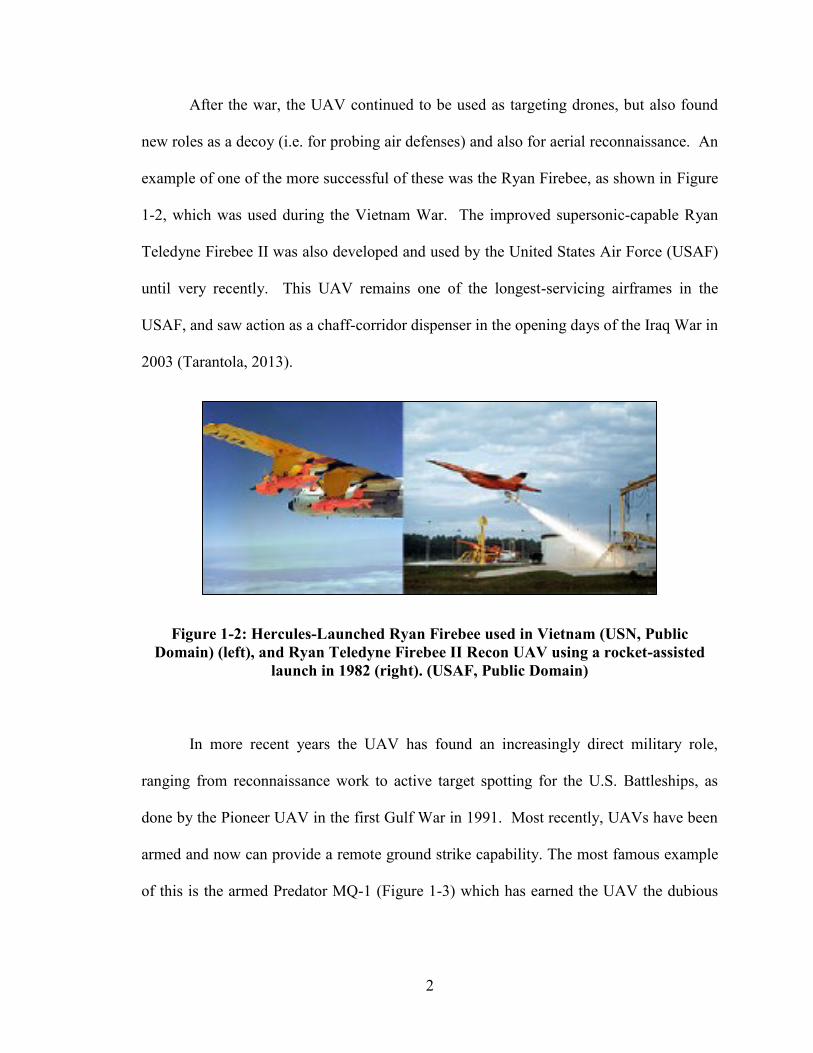
After the war, the UAV continued to be used as targeting drones, but also found
new roles as a decoy (i.e. for probing air defenses) and also for aerial reconnaissance. An
example of one of the more successful of these was the Ryan Firebee, as shown in Figure
1-2, which was used during the Vietnam War. The improved supersonic-capable Ryan
Teledyne Firebee II was also developed and used by the United States Air Force (USAF)
until very recently. This UAV remains one of the longest-servicing airframes in the
USAF, and saw action as a chaff-corridor dispenser in the opening days of the Iraq War in
2003 (Tarantola, 2013).
Figure 1-2: Hercules-Launched Ryan Firebee used in Vietnam (USN, Public
Domain) (left), and Ryan Teledyne Firebee II Recon UAV using a rocket-assisted
launch in 1982 (right). (USAF, Public Domain)
In more recent years the UAV has found an increasingly direct military role,
ranging from reconnaissance work to active target spotting for the U.S. Battleships, as
done by the Pioneer UAV in the first Gulf War in 1991. Most recently, UAVs have been
armed and now can provide a remote ground strike capability. The most famous example
of this is the armed Predator MQ-1 (Figure 1-3) which has earned the UAV the dubious
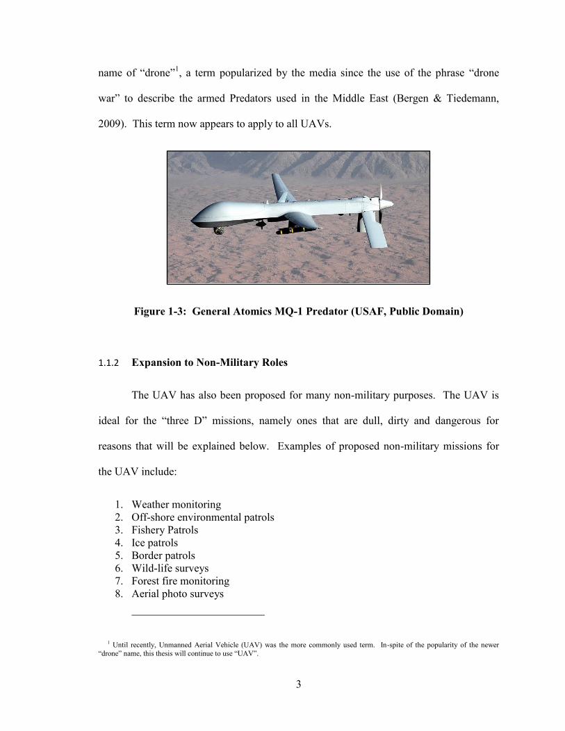
3
name of “drone”1, a term popularized by the media since the use of the phrase “drone
war” to describe the armed Predators used in the Middle East (Bergen & Tiedemann,
2009). This term now appears to apply to all UAVs.
Figure 1-3: General Atomics MQ-1 Predator (USAF, Public Domain)
1.1.2 Expansion to Non-Military Roles
The UAV has also been proposed for many non-military purposes. The UAV is
ideal for the “three D” missions, namely ones that are dull, dirty and dangerous for
reasons that will be explained below. Examples of proposed non-military missions for
the UAV include:
1. Weather monitoring
2. Off-shore environmental patrols
3. Fishery Patrols
4. Ice patrols
5. Border patrols
6. Wild-life surveys
7. Forest fire monitoring
8. Aerial photo surveys
1 Until recently, Unmanned Aerial Vehicle (UAV) was the more commonly used term. In-spite of the popularity of the newer
“drone” name, this thesis will continue to use “UAV”.

4
9. Pipeline surveys
10. Traffic monitoring
11. Communication relays
12. Law Enforcement assistance to police (Levy, 2011)
13. Package deliveries proposed by Amazon (Handwerk, 2013)
14. Food delivery such as the “TacoCopter” (Gilbert, 2012)
Project RAVEN is an example of a proposed use of the Low Altitude Long
Endurance (LALE) class of UAV for the Intelligence Surveillance Reconnaissance (ISR)
missions over the North Atlantic areas off-shore from Eastern Canada (i.e. items 2, 3 and
4 in the previous list). Details on this project are given in Appendix A, which outlines the
proposed Concept of Operations (CONOPS) for the RAVEN Project at Memorial in the
mid-2000s. The primary idea was to use small UAVs to augment what is now done by
Provincial Aerospace Limited (PAL) using manned aircraft like the Beechcraft KingAir.
In this and similar roles requiring close ground inspections, the LALE form of the UAV is
preferred, for reasons which will be elaborated on in the next sections. While there is no
rigorous rule of what defines low-level flight, for the LALE UAV this is certainly less
than 5000 feet (1500m), and more commonly less than 1000 feet (300m).
1.1.3 The Utility of UAVs
Since their inception in the 1940s, the UAV has been used in roles considered too
dangerous or impractical for manned aircraft. The common traits of most operational
UAVs make them ideal for these sorts of missions:
1. DULL – the UAV, having no human pilot or crew to get fatigued, is noted for
having extreme endurance capabilities rivalling the longest-range civilian airliners
or strategic bombers. As an example, a routine mission for the Aerosonde is over
8 hours, and with an extended fuel tank it can fly for in excess of 24 hours

5
(Detailed specs for the Aerosonde Mk4.2 can be found in Appendix B).
Meanwhile, the maximum endurance of a Beechcraft KingAir in the ISR role is
typically around 4-5 hours at low altitudes (Frawley, 1997; Rudkin, 2007). This
extreme endurance makes the UAV ideal for roles requiring it to loiter for hours
on end, or to cover very large distances, both of which will exceed the endurance
limit of any human crew.
2. DIRTY – the UAV is also well suited to fly into situations where the use of a
manned aircraft is impractical or unwise. An early military example was the use of
radio-controlled unmanned aircraft to fly through radioactive fallout clouds during
early nuclear weapons testing in the late 1940s and early 1950s (U.S. Department
of Defense, 2005). A more recent civilian example is forest fire monitoring where
low visibility (smoke) concerns may make the equivalent use of a manned aircraft
too risky, especially at night. Meanwhile the UAV, properly equipped with
Infrared (IR) night vision and flying by autopilot using GPS waypoints, can
operate over forest fires for a full 24 hour period (InsideGNSS , 2013).
3. DANGEROUS – since the UAV has no human crew on board, it may be
considered “expendable” when compared with manned aircraft. This was clearly
the case when it was used as a targeting drone in 1940s or to probe enemy anti-
aircraft defences. A more recent civilian example is the use of the Aerosonde
UAV to fly into the eye of a hurricane. While it is true that the same mission can
be accomplished by manned aircraft, the use of the Aerosonde has found
increasing acceptance due to the obvious lowered risk to crew and airframe plus
the huge cost difference. Even though the Aerosonde is typically sacrificed on
these missions, the cost of an Aerosonde ($100k) is only a fraction the multi-
million dollar price tag of an equivalent Manned Aircraft, and no human lives are
lost. The Aerosonde can also be tasked to stay inside the hurricane for a much
longer duration, and at much lower altitudes then would be considered safe for an
equivalent manned aircraft operation (NOAA, 2005).
6
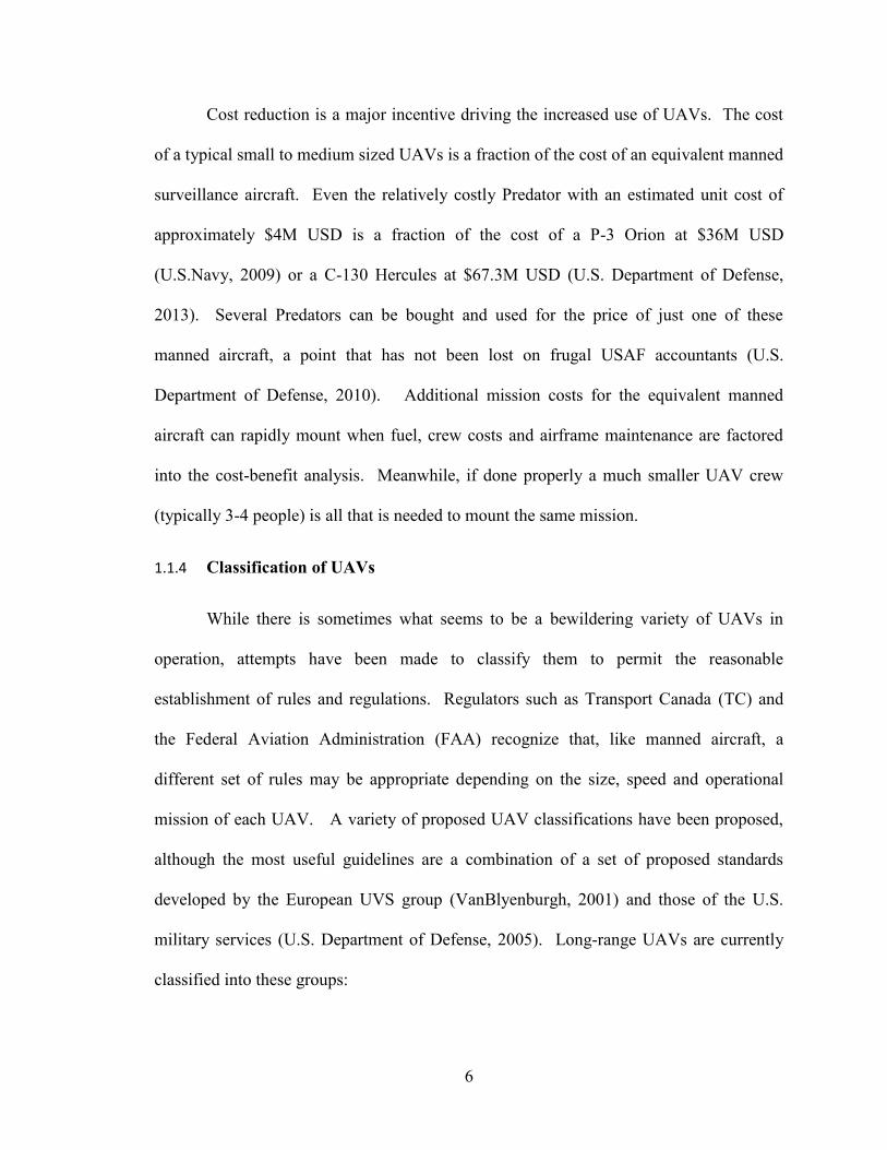
Cost reduction is a major incentive driving the increased use of UAVs. The cost
of a typical small to medium sized UAVs is a fraction of the cost of an equivalent manned
surveillance aircraft. Even the relatively costly Predator with an estimated unit cost of
approximately $4M USD is a fraction of the cost of a P-3 Orion at $36M USD
(U.S.Navy, 2009) or a C-130 Hercules at $67.3M USD (U.S. Department of Defense,
2013). Several Predators can be bought and used for the price of just one of these
manned aircraft, a point that has not been lost on frugal USAF accountants (U.S.
Department of Defense, 2010). Additional mission costs for the equivalent manned
aircraft can rapidly mount when fuel, crew costs and airframe maintenance are factored
into the cost-benefit analysis. Meanwhile, if done properly a much smaller UAV crew
(typically 3-4 people) is all that is needed to mount the same mission.
1.1.4 Classification of UAVs
While there is sometimes what seems to be a bewildering variety of UAVs in
operation, attempts have been made to classify them to permit the reasonable
establishment of rules and regulations. Regulators such as Transport Canada (TC) and
the Federal Aviation Administration (FAA) recognize that, like manned aircraft, a
different set of rules may be appropriate depending on the size, speed and operational
mission of each UAV. A variety of proposed UAV classifications have been proposed,
although the most useful guidelines are a combination of a set of proposed standards
developed by the European UVS group (VanBlyenburgh, 2001) and those of the U.S.
military services (U.S. Department of Defense, 2005). Long-range UAVs are currently
classified into these groups:

7
1. High Altitude, Long Endurance (HALE) – very large UAVs with persistent (24
hr+) with maximum altitudes of about 20,000 m (e.g. RQ-4 GlobalHawk).
2. Medium Altitude, Long Endurance (MALE) - flies for at least 8 hrs, at
altitudes between 5,000-20,000 ft, though these may go lower if required. (e.g.
MQ-1 Predator).
3. Low Altitude, Long Endurance (LALE) – flies at least 8 hrs (many up to 24 hrs)
at altitudes typically under 5000 ft, and most times under 1000 ft (300 m). (e.g.
AAI Shadow200, AAI Aerosonde and Boeing ScanEagle).
UAVs are also classified by size, usually according to maximum takeoff weight
(MTOW). There is some debate over the precise boundary lines between these,
depending on which military service is asked. The accepted classifications as of 2008
were (Bento, 2008):
1. Micro (under 10 lbs)
2. Small/Mini (under 25 kg)2
3. Tactical (25 kg – 1000 lbs)
4. Medium (over 1000 lbs)
5. Heavy (over 10,000 lbs)
The LALE class of UAVs are typically of small to tactical size. Typical examples
are shown in Figure 1-4, including the AAI Shadow 200, Maryland Aerospace VectorP,
AAI Aerosonde and the Boeing ScanEagle.
2 The definition for small UAV varies from 20 kg to 35 kg depending on country/regulator. In this thesis the current Transport
Canada limit of 25 kg will be assumed (TC TP15263, 2014).
8
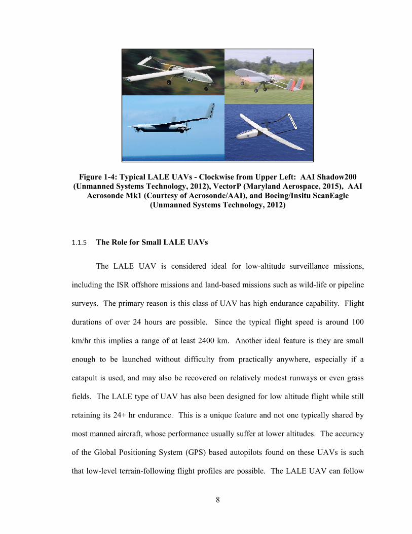
Figure 1-4: Typical LALE UAVs - Clockwise from Upper Left: AAI Shadow200
(Unmanned Systems Technology, 2012), VectorP (Maryland Aerospace, 2015), AAI
Aerosonde Mk1 (Courtesy of Aerosonde/AAI), and Boeing/Insitu ScanEagle
(Unmanned Systems Technology, 2012)
1.1.5 The Role for Small LALE UAVs
The LALE UAV is considered ideal for low-altitude surveillance missions,
including the ISR offshore missions and land-based missions such as wild-life or pipeline
surveys. The primary reason is this class of UAV has high endurance capability. Flight
durations of over 24 hours are possible. Since the typical flight speed is around 100
km/hr this implies a range of at least 2400 km. Another ideal feature is they are small
enough to be launched without difficulty from practically anywhere, especially if a
catapult is used, and may also be recovered on relatively modest runways or even grass
fields. The LALE type of UAV has also been designed for low altitude flight while still
retaining its 24+ hr endurance. This is a unique feature and not one typically shared by
most manned aircraft, whose performance usually suffer at lower altitudes. The accuracy
of the Global Positioning System (GPS) based autopilots found on these UAVs is such
that low-level terrain-following flight profiles are possible. The LALE UAV can follow
9
these flight plans for hours on end without fatigue or impaired pilot judgment causing
problems. The same cannot be said for an equivalent manned aircraft which is forced to
fly at very low altitudes (i.e. 500ft/150m AGL or less) for hours.
1.2 The Challenges and Limitations of UAVs
While there is great interest in expanding the use of UAVs in many non-military
roles, this has been prevented due to a number of deficiencies, both real and imagined,
which have been attributed to UAVs. The most serious is that the UAV, lacking a human
pilot on board, is considered less safe than manned aircraft. This apparent lack of an
Equivalent Level of Safety (ELOS) as manned aircraft is used as a reason to restrict their
operation. This attitude dates back to the Chicago Convention Article 8 (Chicago,
December 7, 1944), which states (ICAO, 2011):
“No aircraft capable of being flown without a pilot shall be flown without a pilot
over the territory of a contracting State without special authorization by that State and in
accordance with the terms of such authorization….”
In Canada, this means a Special Flight Operation Certificate (SFOC) must be
obtained for every UAV operation in Canada (TC SI-623-001, 2014)3. This effectively
prevents the routine use of UAVs for most of the civilian missions proposed.
The specific limitations which appear to be the source of doubts regarding the
safety of the UAV in civilian airspace are detailed in the following sections.
3 There have been very recent developments in both TC and FAA regulations which are a hopeful sign that a balanced approach to
UAV regulations is being followed. In Canada, very recent guidelines have been announced which grants a limited exemption to
several of the CARs related to airworthiness and the lack of a pilot onboard. Two classes of exemptions apply to very small UAVs below 2 kg, and to the small UAVs under 25 kg being considered in this thesis. Provided these are flown below 500 ft AGL and
within visual line of sight at all times, the SFOC requirements have been simplified (TC CAR Exempt., 2014).
10
1.2.1 Lack of Pilot See and Avoid Capability
Since UAVs do not have a pilot on board, the inherent ability implied in the
aviation regulations of the pilot to “see and avoid” other aircraft is absent (FAA AC-90-
48-C, 1983; Henderson, 2010). Of course, the effectiveness of the human “see and
avoid” capability may be questioned (Hobbs, 1991). This perceived deficiency of UAVs
is at the heart of most claims that they are inherently less safe than manned aircraft.
1.2.2 Inadequate Anti-Collision Technologies
The development of appropriate regulations regarding the use of standard anti-
collision equipment on civilian UAVs is very much a work in progress in Canada (UAV
Working Group , 2007), the US (Lacher, Maroney, & Zeitlin, 2007) and the rest of the
world (ICAO, 2011). A detailed discussion will be left for later chapters, although it may
be summarized as follows: simply adopting current standards for manned aircraft, for
example requiring the universal installation of a transponder, navigation and anti-collision
lighting may not be as straight-forward on small UAVs.
Current lighting systems for General Aviation (GA) aircraft such as the Cessna
C172 (35 ft wingspan) may be difficult to fit on the much smaller UAVs like the
Aerosonde Mk4.2. (10 ft wingspan), nor make sense from a geometric point of view (i.e.
light pattern distribution). There is also the problem of power requirements. It is possible
that lighting systems based on ultra-bright LEDs could solve this problem. However,
there are currently no regulations within Canada which define appropriate standards for
vehicles smaller then home-built aircraft such as the Murphy Rebel, considered to be in
the “Ultra Light” class at 1650 lb, 30 ft wingspan (Murphy Aircraft, 2008).

11
There is also confusion over the need for a transponder. In Canada, the legal
requirement is that a transponder is needed only if an aircraft will fly into Controlled
Airspace. The rules for U.S. Airspace are similar (MacDonald & Peppler, 2000).
Generally speaking this is airspace above a certain altitude or within an Air Traffic
Control (ATC) control zone. LALE UAVs are normally used for missions at very low
altitudes and in remote locations far from major population centers. Unless the mission
requires them to launch and recover at a major airport, they are unlikely to fly into
controlled airspace.
As a result of this uncertainty regarding lights and transponder requirements, the
general response by small UAV airframe manufacturers is to simply omit them. The
customer then assumes the responsibility to make any necessary modifications according
to local regulations. This is the case with the Aerosonde Mk4.2, the VectorP and the
TBM UAV1. All are supplied without lights or a transponder. Our own experience is
that in the absence of regulations for small UAVs, the regulator will make rulings on a
case-by-case basis and typically err on the side of stricter requirements than for manned
aircraft.
1.2.3 No Detect, Sense and Avoid System
Most current UAVs are essentially “blind” during autonomous flight and have no
awareness of other potential airborne or ground-based collision hazards. This situation
will persist unless some form of autonomous Detect, Sense and Avoid (DSA) system is
provided. At present a system suitable for use in the smaller LALE class of UAVs is
unavailable (Davis, 2006). This poses a serious risk and concern, and is a major limiting
12
factor to UAVs gaining general acceptance by aviation regulatory bodies and amongst
pilots (Kirkby, 2006).
Without a reliable DSA capability that provides an ELOS as manned aircraft,
small UAVs will be regarded as a threat to flight safety. Flight operations for UAVs in
Canada are currently only allowed through advanced application and approval of an
SFOC (TC SI-623-001, 2014). There are restrictions limiting operational times (i.e.
typically these are daytime visual weather conditions), their ability to fly in controlled
airspace and to fly Beyond Line of Sight (BLOS). These restrictions are contrary to the
type of routine operations in non-segregated airspace implied by the proposed missions
for small LALE UAVs.
1.2.4 Limited BLOS Situational Awareness
Most UAVs, especially the smaller LALE class, have limited Beyond Line of
Sight (BLOS) situational awareness capabilities. This could be considered an element of
the DSA problem but what we are mainly talking about here is the awareness of the
Autonomous Vehicle Operator (AVO) whose job it is to control and monitor the UAV at
the Ground Control Station (GCS). Most commercial GCS software packages used with
small UAVs do an excellent job of showing what the UAV is doing, assuming a good
telemetry link is maintained. The GCS usually shows a plan view in the form of a 2D
map with the current waypoints, UAV location and some track history displayed. An
example is shown in Figure 1-5, in this case the Mission Planner GCS used in conjunction
with the ArduPilot (3D Robotics, 2014). In this annotated example provided by 3D
Robotics, the key elements of the display are detailed. Similar displays are present in the

13
Horizon GCS used with the MicroPilot and the Cloud Cap GCS used with the Piccollo II
autopilot as installed on the Aerosonde.
Figure 1-5: APM Mission Planner GCS Display with Annotations
(courtesy of 3D Robotics)
Only those UAV(s) under the direct command of the local GCS are typically
shown in current commercial GCS software suites. The AVO is usually unaware of any
other entities which are not under his direct control. This could include other UAVs,
ground or terrain obstacles, or manned aircraft which might also be in the vicinity.
Attempts have been made to augment the situation using some other means such as
Automatically Dependent Surveillance-Broadcast (ADS-B) and this is an active research
area. However, this information is usually on a separate display, not integrated into the
GCS and thus very difficult to use for precise coordination, especially at BLOS ranges.
14
Unless these different data streams are fused together into a single, cohesive situation
display at the GCS, the overall situational awareness will be very limited.
1.2.5 Unique Challenges for the Small LALE
While the small LALE type of UAV is an ideal candidate for the ISR missions,
they have a number of unique challenges in addition to those already discussed.
1.2.5.1 Low visibility
The small LALE UAV is typically an airframe with a wingspan of around 10 ft
(3m) and very narrow fuselage under 1 ft (0.3m) diameter. The forward cross-sectional
area, optimized for low drag and endurance unfortunately has the side-effect of creating
an airframe that is very small and difficult to see at normal aviation sighting distances.
The small UAV is essentially invisible to other aircraft without some form of visual
enhancements.
1.2.5.2 Limited Payload
The small LALE UAV, typically with a maximum takeoff weight of under 15 kg
(30 lbs), has a very limited payload, typically in the 5-7 kg (10-15 lb) range, including
fuel. This limits what can be carried by the UAV, especially in terms of anti-collision
and detection equipment. For example, there is no known radar system light or small
enough that would fit on existing small UAVs. This is the primary reason why no system
has yet been developed that would fit on the small UAV and provide the required DSA
capabilities (Ellis, Investigation of Emerging Technologies and Regulations for UAV
‘Sense and Avoid' Capability, 2006).
15
1.2.5.3 Manual Control Methods
Current TC regulations require that even in the case of fully automatic UAV
flight, there exist a manual override capability throughout the flight, equivalent to the
implied Pilot-in-Command capabilities on manned aircraft. This requirement for a human
“Safety Pilot” is expected to remain in the regulations for many years to come (TC SI-
623-001, 2014). Unfortunately, the current Radio Control (R/C) manual pilot method
used by most small UAVs is not suitable for several reasons.
The most obvious problem is that manual R/C control methods restrict control to a
very limited visual range from the airfield, perhaps 0.5 km maximum. This is contrary to
the nature of the long range missions that the LALE UAV is most suited to perform. It is
possible to augment this method somewhat by switching to remote operation of the UAV
using a forward-looking video camera, also called the First Person View (FPV). This is a
commonly employed technique with larger military UAVs like the Predator (USAF,
2010). We have demonstrated a similar capability on the Aerosonde Mk4.2 using much
smaller and lighter analog video transmission equipment. However this mode is only
possible within electronic Line-of-Sight (eLOS) conditions, meaning the range in which a
high speed video and telemetry link is possible, which is typically a maximum of 20 km
range. Note that the precise real-time operation of a UAV will be hampered if not
impossible if satellites are used, due to increased data link latency and/or bandwidth
limitations (Clough, 2005).
Another problem is personnel availability and skill set. It is incorrect to assume
that any manned aircraft pilot can successfully fly a small UAV remotely, especially if the
16
R/C mode is used. The nature of R/C control, where you are viewing the aircraft
externally (as opposed to from within the cockpit), requires a different skill set than with
manned aircraft. Common problems include over-control and pilot disorientation due to
“control reversal” caused when the aircraft is facing the R/C pilot. Another problem,
experienced by this author personally, is in rapidly determining the aircraft orientation
when the small aircraft is far away or under rapidly changing or difficult lighting
conditions (e.g. sunlight glare or airplane silhouetting). A FPV video might alleviate
most of these pilot disorientation effects, but there is still the issue of over-control. This
is especially true for the smaller LALE class of UAV, where the flight dynamics are
similar to the larger acrobatic gas-powered R/C hobby aircraft. The control of these
model aircraft requires extremely gentle control inputs and fast reflexes. It is a skill that
takes years to develop and one which some may never master. This creates a serious
personnel training paradigm (Williams, 2004).
Another concern with manual piloting is the requirement for the LALE UAVs to
fly in less-than-ideal weather conditions, for example if used in the ISR role in the North
Atlantic maritime environment. Current manual piloting practice will restrict flight
operations to relatively benign weather conditions. There are limits on crosswinds and
visibility, which on small airframes is even more restrictive than the rules for the smallest
General Aviation (GA) aircraft. The manual pilot is simply not fast enough to control a
small UAV safely in adverse wind conditions, and completely incapable of piloting a
vehicle in poor visibility conditions. Without remedy, this is a major restriction to
operational use of small UAVs for realistic maritime conditions.
17
1.3 Problem statement
This research project has attempted to assess the current risk imposed by the small
UAV in order to determine its current Estimated Level of Safety (ELS). By comparing
this with manned aircraft we may determine if it is possible to improve the UAV, using
novel technologies or operational methods to give is an ELOS as manned aircraft
operating in the same airspace.
1.3.1 Risk Assessment
The addition of the small UAV to the same airspace where manned aircraft will
also fly (i.e. non-segregated airspace) does create a number of additional risks. The real
physical risks are:
1. Ground Collision Risk – This is the risk the UAV poses to people or property on
the ground due to the UAV crashing or colliding with the ground. This could be
due to equipment failures, environmental or operational errors which cause the
UAV to strike the ground in either an un-controlled crash or controlled flight into
ground obstacles. Environmental factors could include the onset of poor weather
which may lead to equipment failure if not properly designed-for in the airframe.
Bird-strikes are another source of damage. There is a need to improve the take-off
and landing phases, especially for over-loaded small UAVs, to reduce the
incidence of airframe losses at these critical stages. Proper planning for
emergency landing procedures due to in-flight damage (i.e. from bad weather or
bird-strikes) is also required.
2. Mid-Air Collision Risk - This is the additional risk of an air-to-air collision due
to the addition of the UAV into the airspace. This is directly associated with
presence (or lack) of anti-collision technologies, including DSA, on the small
UAV.

18
There are also perceived threats or risks due to UAV operations, both real and
imagined, which limit their acceptability and ability to gain approval to be used in many
of the civilian mission roles. Some of these may be difficult to correct but we must be
aware of them:
1. Fear of UAVs as being an invisible, non-compliant user of the airspace, especially
amongst pilots (Kirkby, 2006).
2. Public fear of the UAV as “drones” in the sense of the Predator usage by the U.S.
to conduct targeted killings in the Middle East. The negative publicity of this
recent use of “drones” has tainted the public perception of all UAVs. (Bergen &
Tiedemann, 2009; Haven, 2011) There have also been recent concerns over
privacy especially with the surge in the popularity of the small hobby drones
(Brown, 2014).
3. Limited reliability data (for civilian UAVs) due to their very recent history,
especially when compare with equivalent manned aircraft which now has many
decades of statistic data to validate their safety. This is a major source of the
generally conservative stance being taken by aviation regulators worldwide
regarding UAV airworthiness.
1.3.2 Definition of Equivalent Level of Safety
This research project has concentrated on one of the more difficult aspects of the
UAV safety problem, and the subject of much debate within the UAV industry and
amongst government aviation regulators – the concept of “Equivalent Level of Safety”
(ELOS). It is interesting that the concept of ELOS is used without much quantification of
what it means. All would agree that the basic interpretation is essentially that the UAV
must be at least as safe as manned aircraft in the same airspace (NATO Naval Armaments
19
Group, 2007). Unfortunately, this is usually where agreement ends, since the definition
of manned aircraft safety is itself open to some debate (Hobbs, 1991).
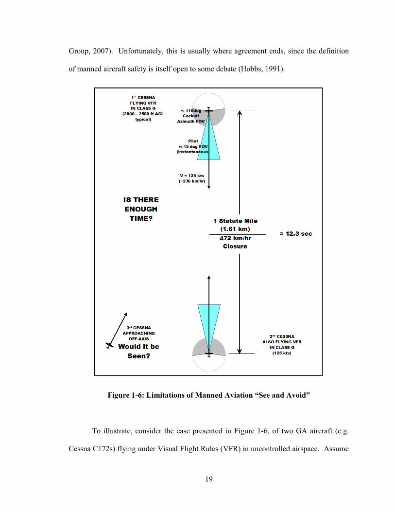
Figure 1-6: Limitations of Manned Aviation “See and Avoid”
To illustrate, consider the case presented in Figure 1-6, of two GA aircraft (e.g.
Cessna C172s) flying under Visual Flight Rules (VFR) in uncontrolled airspace. Assume
20
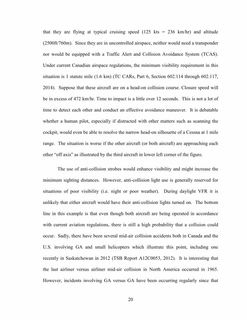
that they are flying at typical cruising speed (125 kts = 236 km/hr) and altitude
(2500ft/760m). Since they are in uncontrolled airspace, neither would need a transponder
nor would be equipped with a Traffic Alert and Collision Avoidance System (TCAS).
Under current Canadian airspace regulations, the minimum visibility requirement in this
situation is 1 statute mile (1.6 km) (TC CARs, Part 6, Section 602.114 through 602.117,
2014). Suppose that these aircraft are on a head-on collision course. Closure speed will
be in excess of 472 km/hr. Time to impact is a little over 12 seconds. This is not a lot of
time to detect each other and conduct an effective avoidance maneuver. It is debatable
whether a human pilot, especially if distracted with other matters such as scanning the
cockpit, would even be able to resolve the narrow head-on silhouette of a Cessna at 1 mile
range. The situation is worse if the other aircraft (or both aircraft) are approaching each
other “off axis” as illustrated by the third aircraft in lower left corner of the figure.
The use of anti-collision strobes would enhance visibility and might increase the
minimum sighting distances. However, anti-collision light use is generally reserved for
situations of poor visibility (i.e. night or poor weather). During daylight VFR it is
unlikely that either aircraft would have their anti-collision lights turned on. The bottom
line in this example is that even though both aircraft are being operated in accordance
with current aviation regulations, there is still a high probability that a collision could
occur. Sadly, there have been several mid-air collision accidents both in Canada and the
U.S. involving GA and small helicopters which illustrate this point, including one
recently in Saskatchewan in 2012 (TSB Report A12C0053, 2012). It is interesting that
the last airliner versus airliner mid-air collision in North America occurred in 1965.
However, incidents involving GA versus GA have been occurring regularly since that

21
time. There have also been several incidents where a GA aircraft collided with a
commercial airliner, perhaps the most infamous being the 1986 Aero-Mexico mid-air
collision over Cerritos, which resulted in catastrophic casualties including many on the
ground (NTSB/AAR-87/07, 1987). In all of these incidents, the NTSB accident report
invariably reaches the same conclusion: that pilot error, and the inherent limitations of the
“see and avoid” principle in manned aircraft were to blame.
The limitations of the “see and avoid” principle in manned aircraft have been
documented by many researchers and known for many years (Graham & Orr, 1970).
These limitations were summarized in an Australian Report in 1991 (Hobbs, 1991). The
recognition of these limitations was the main incentive towards the research and
development of automatic collision avoidance systems in the late 1960s to 1980s, and the
reason why we have the TCAS system as standard equipment on all commercial air traffic
today. The Aero-Mexico mid-air collision in particular, and its similarity to another
incident near San Diego in 1978 was what finally spurred action by the FAA to make
TCAS mandatory by 1993 (FAA AC-120-55-A, 1993). This has clearly made civilian
airline transportation quite safe, but the situation with smaller GA aircraft remains
essentially unchanged, as the accident in Saskatchewan in 2012 demonstrates.
1.3.3 Summary of the Detect Sense and Avoid Problem
Table 1-1 summarizes the combinations inherent in the DSA problem, assuming
Visual Meteorological Conditions (VMC) exist. The first quadrant (1) represents the
situation with manned aircraft, where every pilot is responsible to maintain vigilance for

22
other aircraft and provide the collision avoidance capability. The limitations of the “see
and avoid” principle does cast some doubt on the overall safety of this situation.
Table 1-1: Summary of the DSA Problem for Small UAVs in VMC
Intruder Type
Aircraft
Type
Manned UAV
Manned (1) Manned VFR Flight (2) Can the UAV be seen
and avoided?
UAV (3) Can we see and avoid
manned aircraft?
(4) Cooperative UAVs
Quadrant four (4) represents the other extreme where multiple UAVs in the same
airspace must see and avoid each other. This is technologically the easiest situation to
remedy. There are GPS-based systems which can cooperatively broadcast position
information to other similarly-equipped air vehicles and coordinate avoidance maneuvers,
such as ADS-B (Contarino, 2009). Provided all UAVs in the area use such a system,
implementation of an autonomous DSA system becomes fairly straightforward.
Quadrants two (2) and three (3) represent the challenge for small UAVs, and the
focus of research in the DSA field. In the case of quadrant 2, this is the concern of
whether the UAV represents a collision (obstacle) hazard to manned aircraft. Small
UAVs are more difficult to see then the smallest manned aircraft. Quadrant 3 represents
the problem in the other direction (i.e. “Can the UAV see and avoid manned aircraft?”)
and defines the basic problem of DSA, especially if both cooperative and un-cooperative
aircraft must be considered. The UAV must be able to sense intruding vehicles and other

23
collision hazards in the airspace, and possess some autonomous collision avoidance
capability. However, at present there are no DSA systems recognized by any aviation
regulatory body as providing a small UAV with an equivalent level of safety as that of
manned aircraft (Ellis, Investigation of Emerging Technologies and Regulations for UAV
‘Sense and Avoid' Capability, 2006).
1.4 Thesis Outline
This first chapter has provided an introduction to the topic of small UAV safety.
The motivation driving the use of UAVs, and specifically the small LALE class of UAV,
has been presented along with a summary of the challenges which currently limit their
acceptability and use in civilian airspace. The research in this thesis attempts to assess
the current level of safety of the small UAV. Ways to mitigate the real or perceived risks
posed by the small UAV will be explored in the following chapters, which are organized
as follows.
In Chapter 2 a qualitative measure of the perceived risks associated with UAVs is
presented. This is followed by a quantitative estimate of the real risks that the UAV
poses, primarily in terms of the threat to the ground (i.e. Ground Impact risk) and other
aircraft (Mid-Air Collision risk). This allows an assessment to be made of the ELS of the
small UAV.
Chapter 3 presents research into methods to reduce the ground impact risk by
improving the controllability and situational awareness while operating small UAVs.
This research includes the use of Virtual Reality technologies to fly small UAVs using
FPV techniques, and possible long-range enhanced control methods. Reductions in the
24
mid-air collision risk may also be possible, especially when enhancements to AVO
situational awareness are considered.
Chapter 4 addresses the air-to-air risk pertaining to small UAV visibility, starting
with theoretical calculations of the limits to detection range by human pilots. The chapter
presents results from a series of night time and day time visibility experiments using
lights, and the results of field testing of other visibility enhancement technologies. This
research primarily concerns the “can the UAV be seen?” concern noted in Quadrant 2 of
the DSA summary given in Table 1-1, its effect on the mid-air collision risk, and possible
ways to mitigate this risk.
Chapter 5 presents research into 4D simulation and a theoretical discussion of
various 4D maneuvers and possible avoidance methods. This addresses the mid-air
collision risk implied in Quadrants 2 and 3 of Table 1-1. However, it should be
recognized that the development of a reliable and autonomous DSA capability that
addresses the concerns of manned aviation will involve a multiple-step approach,
including:
1. Theoretical analysis;
2. Simulation of DSA scenarios;
3. Field testing, including data collection, using UAV versus UAV techniques;
and,
4. Field testing involving manned aircraft.
This is a very large subject area, so by necessity this thesis has focused on the first two
steps. In addition to an accurate 4D simulation environment, a novel method to test DSA
strategies and a very promising collision avoidance method are introduced. This lays a
25
strong foundation for the field testing implied in Step 3. It is hoped that the methods
presented might be used during live UAV field testing in the near future, and provide
validation, experience and confidence in the proposed DSA methods. The experience and
confidence gained during Step 3 are essential before contemplating the live testing
involving manned aircraft as implied in Step 4.
Chapter 6 is the conclusion of this thesis. It summarizes the risk assessments from
previous chapters and the potential improvements possible by adopting the mitigation
strategies presented in this thesis. A minimum set of requirements for a DSA system
suitable for small UAVs is presented. The chapter provides the summary of the current
situation related to UAV safety, and in particular very recent developments in this area.
The thesis concludes with some recommendations for follow-on research topics.
26
Chapter 2 Assessing the Risks Posed by UAVs
In this chapter we will discuss both the perception and the reality of the risk posed
by the UAV, and in particular the small UAV4. An attempt will be made to determine the
real threat level posed by the small UAV in a quantitative manner, especially in terms of
the Ground Impact and Mid-Air Collision risks. The other “political” concerns will also
be discussed. Only when an objective comparison is made with manned aviation can we
determine whether or not the small UAV has an ELOS as manned aircraft. With this
knowledge we will be in a much better position to assess if the small UAV meets, exceeds
or falls short of the safety expectations imposed on it. From this analysis we will then be
able to determine where efforts should be focused so that the safety of the UAV may be
improved. In the following discussions, several different aviation regulations will be
mentioned. Excerpts from the Canadian Aviation Regulations (CARs) applicable to this
safety discussion are provided in Appendix C.
2.1 The Requirements for UAV Integration
Even though Unmanned Aerial Vehicles are recognized to be a very effective tool
for many civilian missions, their acceptance by aviation regulators is prevented by the
perception that they are not mature enough to be properly integrated into the busy national
airspace systems of most countries. Specifically, there are many regulatory restrictions
4 It should be recognized that the UAV must be considered as a system – including not just the obvious airframe but also the avionics, GCS and operational procedures. In the following discussions, while much of the risk assessment focuses on the obvious
airframe hardware, mention will also be made of other potential sources of problems, especially operational concerns. And while
software-induced failures will not be described in detail, they will be considered as being included in the overall reliability estimates for typical small UAVs.
27
which prevent the routine operation of UAVs. Routine operations are essential for UAVs
to be both cost-effective and an advantage over equivalent manned operations.
There are active efforts to determine what must be done to permit this to happen.
Very recently, the U.S. Federal Aviation Administration (FAA) presented its updated
roadmap for the integration of Unmanned Aircraft Systems (UAS)5 in the National
Airspace System (NAS). The forward from FAA Administrator Michael Huerta sets the
tone (Federal Aviation Administration, 2013):
“This roadmap outlines the actions and considerations needed to enable UAS
integration into the NAS. The roadmap also aligns proposed FAA actions with
Congressional mandates from the FAA Modernization and Reform Act of 2012. This plan
also provides goals, metrics, and target dates for the FAA and its government and
industry partners to use in planning key activities for UAS integration.”
The FAA roadmap provides detailed information on what is deemed necessary to
allow all this integration to happen. The following excerpt in the FAA roadmap, taken
from the International Civil Aviation Organization (ICAO) circular for UAS summarizes
the requirements very well (ICAO, 2011):
“A number of Civil Aviation Authorities (CAA) have adopted the policy that UAS
must meet the equivalent levels of safety as manned aircraft… In general, UAS should be
operated in accordance with the rules governing the flight of manned aircraft and meet
5 The FAA uses the more generic term Unmanned (or Uninhabited) Aircraft System (UAS), to define the UAV as being a system which includes not only the airframe but also the ground-based control systems and operators. However this thesis will continue to use
the more generic acronym UAV.

28
equipment requirements applicable to the class of airspace within which they intend to
operate…To safely integrate UAS in non-segregated airspace, the UAS must act and
respond as manned aircraft do. Air Traffic, Airspace and Airport standards should not be
significantly changed. The UAS must be able to comply with existing provisions to the
greatest extent possible.”
Thus the basic definition of ELOS may is summarized as this: the UAV must
possess the same inherent safety as manned aircraft, and operate in a similar manner, to
be allowed to operate freely in non-segregated airspace. Another significant FAA
statement relates to the need for the UAV to mature significantly in terms of
airworthiness:
“Except for some special cases, such as small UAS6 with very limited operational
range, all UAS will require design and airworthiness certification to fly civil operations
in the NAS.”
In Canada, Transport Canada (TC) set up a UAV Working Group in the mid-
2000s to make recommendations for changes required to the Canadian Air Regulations
(CARs) to allow UAVs to operate in segregated and non-segregated airspace. Consensus
among the UAV Working Group members was that the growth area in UAV operation
will be in the small class of UAVs. These aircraft are extremely capable, having a service
ceiling of 6,000 m, flight duration exceeding 24 hours and an operating range of many
6 The small UAS being mentioned here is equivalent to modified R/C aircraft equipped with an autopilot, typically flown within 1 km of its landing area.

29
thousand kilometers. An example is the Aerosonde Mk4.2 UAV, detailed in Appendix B.
This class of UAV was deemed problematic since their small size and light weight
precludes the use of existing off-the-shelf systems such as TCAS. A report was generated
with regulations to follow after technical and legal review (TC UAV Working Group,
2007). It was hoped this would eliminate the regulation bottleneck preventing routine
UAV operations in Canada. As recently as two years ago, the development of CARs
specifically for UAVs had stalled. However, the recent surge in “drone” usage has
revived efforts by regulators to define appropriate UAV regulations. An updated SFOC
staff instruction was issued by TC only this past November (TC SI-623-001, 2014). TC
still considers each UAV application on a case-by-case basis, requiring an SFOC for each
and every UAV mission, although exemptions are possible for very small UAVs operated
solely within visual line of sight (TC CAR Exempt., 2014).
Internationally, there have been attempts since 2005 by various international
organizations to develop standards and regulations regarding the operation of UAVs, and
the requirements for DSA technologies. The absence of a viable DSA technology which
may be used by civilian UAVs was considered as the main obstacle (Ellis, Investigation
of Emerging Technologies and Regulations for UAV ‘Sense and Avoid' Capability,
2006). The most comprehensive of these were the European Eurocontrol (2006), the
American ASTM-F2411-04 Committee, and the NATO Joint Capability Group on
Unmanned Aerial Vehicles. The Eurocontrol committee focused on specifications for
military operational air traffic and some recommendations have been adopted selectively
for GA traffic (Eurocontrol, 2006). The ASTM committee focused on performance-based
30
standards, but the recommended certification procedures involve costly flight tests and
simulation runs due to the combinatory nature of the required test scenarios. The NATO
Group generated a comprehensive set of requirements for collision avoidance and general
operating rules applicable to UAVs over 150 kg, with the goal of establishing a set of
international standards applicable amongst its member countries (NATO Naval
Armaments Group, 2007).
As of this writing, there still remains to be seen a definitive set of regulations
applicable to UAV integration. It would appear that many are taking a “wait and see”
attitude, likely hoping for some breakthrough in DSA technology or the FAA taking a
leadership role and spearheading the establishment of such regulations (Murfin, 2013).
2.2 Perceived and Assumed Risks
There are a number of perceived and assumed risks associated with the operation
of an UAV that we have encountered during our initial flight test of several small UAV
systems, including the Aerosonde UAV. The fear of these perceived risks hamper the
acceptance of UAVs and the practical aspects of flight operations have dampened the
initial enthusiasm and assumptions of lowered operational costs.
2.2.1 Risk to the Crew
While the airborne operation of the UAV does not pose any threat to a crew on-
board the aircraft, there is a small risk to the operators on the ground, particularly during
the launch and recovery stages. This is particularly true when manual R/C flying
techniques are used. The threat of injury to a member of the ground crew increases with
31
crew size, so it is incumbent on the UAV operator to limit the number of personnel at the
airfield. It is also important to minimize (or eliminate altogether) any non-involved
spectators who may be interested in watching the UAV operation. The danger is the
small UAV resembles a large R/C aircraft and thus both the operator and bystanders can
become complacent about the risk. As an example, the Aerosonde UAV lands at a very
high speed, approximately 80-90 km/hr and has a set of very narrow wings similar to
propeller blades. During the final stage of landing the Aerosonde is an unpowered glider
approach, meaning it will be coming in to land somewhere after the commitment time
when engine power is cut, and has limited maneuvering options. If this UAV were to hit
someone standing beside the runway, it would most certainly injure them badly, perhaps
fatally.
This is an issue which the R/C hobby has had to deal with in recent years
especially after several incidents in Europe and Canada where spectators were injured (or
killed) while watching R/C flying events (MTI Hungary, 13 May 2006). Adopting a
minimum safe distance from spectators, similar to existing R/C air field guidelines in the
Model Aeronautics Association of Canada (MAAC) or the Academy of Model
Aeronautics (AMA) would also be wise to prevent any incidents involving spectators
(MAAC, 2014).
For the ground crew, this risk is easy to reduce simply by adopting prudent safety
practices at the airfield. In the case of the Aerosonde, requiring that all personnel take
cover (e.g. going inside the GCS van or another vehicle) during the launch and recovery
stages of the mission would be sufficient to eliminate this threat.
32
2.2.2 High Operational Costs
During initial UAV operations, especially by people accustomed to manned
aviation, there is a tendency to apply manned aviation practices to the small UAV. This is
particularly true in terms of the number of people in the cockpit, number of sensor
operators, maintenance personnel and so forth. Whereas most small UAV vendors quote
crews of 2-3 required to operate them, this author has personally witnessed the growth of
the Aerosonde UAV crew to as much as a dozen people at a given time. This mode of
operation might be necessary during the initial training stages, but must transition to a
leaner operating model very quickly, or the economic case for using the UAV will be
defeated. The high initial training and start-up costs with our Aerosonde UAV operations
was a major reason why this portion of the project to stall.
The operation of the small UAV should be possible with only three people: a
manual (safety pilot) who also performs much of the maintenance duties, the AVO who
will monitor and control the autopilot portion of the mission, and a mission supervisor
whose responsibility would be to ensure the SFOC rules are being observed and is
prepared to communicate with other airspace operators using an Air-band radio.
2.2.3 Financial Risk due to Attrition
Another hurdle to UAV acceptance is the fear of losing the aircraft, and the
associated financial cost. In 2006 we had been warned by the Aerosonde UAV vendor to
expect some attrition in our UAV fleet, especially as flight hours increased. This is an
admission that though a very thorough flight checkout procedure preceded every

33
Aerosonde mission, there were still real concerns over the reliability of the airframe,
especially in terms of the radio link between the UAV and the GCS, and with the engine.
We experienced the loss of two airframes, and both incidents were associated with a loss-
link between the manual pilot and airframe. Recently, the Aerosonde UAV power-plant
underwent a thorough re-evaluation after concerns over its reliability surfaced with
increasing utilization with the U.S. military (Rosenberg, 2013). This problem is common
in civil aviation, especially with novel systems or engines. It is only once an airframe
starts to accumulate a high number of hours that quality problems will surface, and the
outcome of reliability estimates (a routine task performed for engines and sub-systems)
are validated. The Aerosonde powerplant problems were solved after a major manned
aircraft engine manufacturer (Lycoming) stepped in and applied civil aviation methods
(Hemmerdinger, 2013).
Especially at the initial stages of small UAV operations, the loss of airframes due
to flight mishaps will have a direct impact on the operating costs of the program, and will
also have the practical effect of decreasing the availability of aircraft to perform missions.
Both concerns are seen to be major drivers behind the “fear factor” preventing the use of
the small UAV for the risky LALE missions for which it was designed to perform.
Based on our own experience, before embarking on a program using commercially
available small UAVs, the attrition cost due to loss of airframes must be considered and
planned for, and then monitored carefully as the project progresses. This is important
later when there may be a need to prove the reliability of the system (e.g. when applying
for an SFOC). It is wise to assume the loss of an airframe as occurring at a particular rate.
34
The best source of information in these situations is to contact another user of the same
UAV, one who has used it for enough hours to permit a realistic assessment of its
operational reliability.
2.2.4 The Doctrine of Zero-Tolerance
Until small UAVs improve in terms of quality and reliability, it is a foregone
conclusion that they will crash. This is where their operation runs afoul of the doctrine of
zero-tolerance to incidents or accidents which exists (for good reason) in manned
aviation. Aircraft operators accustomed to this doctrine follow a similar conservative
stance built-in to manned aviation culture. This is a good thing for manned aviation, but
unfortunately is counter to one of the main reasons to use UAVs – that they may be
considered expendable and used for very risky missions where a crash may very likely be
the final outcome. It is true that to maintain the cost benefit of using UAVs, it is still
prudent to prevent needless airframe losses during routine operations, for example during
takeoff and landing where most of the serious incidents typically occur.
What must be realized is that the civilian UAV is a relative newcomer to aviation,
perhaps having only 15 years’ experience. Manned aviation is now over a century old but
it too experienced much of the same growing pains, crashes, blunders and tragedies,
especially in the early years. The key point is that manned aviation learned from these
early mistakes and experiences, steadily improving the technology and operational
techniques used. The net result is that modern air travel is statistically the safest form of
transportation today (ICAO, 2013).

35
For the UAV to gain acceptance, especially with regulators, it must be allowed to
fly with increasing frequency to allow operators to gain the knowledge and experience
needed to improve them and make them safer. The fear of crashing must be replaced
with a prudent acceptance of failure. Until the small UAV matures and reliability
improves, UAVs must be designed and operated with the assumption that it may crash at
any moment. Operational procedures and the airframes must be designed with this in
mind, always with the aim to minimize the risk, especially to people or property on the
ground, and also to mitigate the effects of a crash. Only once a given small UAV has
been flying for a large number of hours (i.e. 10,000+ hrs) without serious incidents will
this perceived risk be reduced.
2.2.5 Public Fear of UAVs
Public fear of the UAV was not a major concern when civilian UAV operations
were first contemplated in the early 2000s. However, recent negative publicity, especially
the controversy over the use of the Predator-B as a hunter-killer asset in the Middle East
has not helped the case for the UAV (Bergen & Tiedemann, 2009). There seems to be a
growing public perception that the “drone” is to be feared, either as a direct threat to life,
or as an invasion of privacy for some of its proposed surveillance roles.
Unfortunately there is not much we can do (technically) to dispel this perception,
apart from ensuring that our operations do not create any threats to people on the ground
or other aircraft. Public education into the advantages of the civilian UAV is also needed
to combat the negative perception of the evil “drone”. This is a critical time. In a recent
36
article in the AUVSI journal (Haven, 2011), the danger to the future of the UAV industry
was compared to that of the nuclear industry, which is essentially gone in North America
due to poor public perception coupled with the unfortunate timing of several nuclear
accidents. The same thing could happen with UAVs in the current negative political
environment.
Once UAVs are operating and providing reliable services, as package delivery
systems for Amazon, assistance to fire or police emergencies, or as friendly traffic alert
systems in the sky for motorists, public acceptance of the presence of the small UAV in
civilian areas should improve. The one thing that can be done in the meantime is to
strive to improve the reliability of the small UAV to prevent any incidents, and to design
operations to minimize any risk the UAV may pose to the general public.
2.2.6 Motivation for Improved Reliability
Much of the perceived risks (fears) associated with UAVs, and in particular the
small UAV, may be reduced or eliminated through improved reliability of the airframe
and the overall UAV system. Improving the reliability of the airframe should help
reduce airframe attrition rates and drive down costs associated with operations due to lost
aircraft. Overall improved quality of the airframe should also reduce the excessive
amount of maintenance that is currently needed on some small UAVs to maintain even a
modest level of reliability. Improved reliability of the overall UAV system will likewise
reduce the number of incidents and help improve the public perception of the UAV as a
safe user of the air space above their heads. Aviation regulators and other manned aircraft
37
operators alike will also improve their perception of the risk the UAV poses, and allow it
greater operational freedom.
2.2.7 The Motivation for UAV Control Enhancement Research
Another area of improvement is in the area of operations, specifically how the
small UAV is controlled during take-off and landings. It is proposed that much of the
current safety concerns of small UAV operations, in particular the safety of the ground
crew and airframe, may be alleviated if a different mode of operation is used. The manual
R/C method of flying these UAVs may not be the most effective nor safest method. The
use of Automated Take-off and Landing (ATOL) technologies could have a beneficial
impact, reducing incident rates of crashes during these critical flight phases. This would
also help alleviate much of the stress currently encountered with R/C pilots, especially
when they are forced to fly small UAVs at close to their operational limits and in
challenging weather conditions. An effective ATOL capability could allow UAV
operations in poor (i.e. non-VMC) weather conditions, equivalent to the use of the
Instrumented Landing System (ILS) by manned aircraft flying under Instrument Fight
Rules (IFR).
Even if a full ATOL method is not yet available, it is proposed that the use of
alternative control methods such as FPV flying techniques may be a safer approach,
particularly during the landing stage. Eliminating the need to have a manual pilot
standing on the side of a runway, especially during the landing of the faster small UAVs
like the Aerosonde, should be considered. An alternative method whereby the pilot sits

38
inside the GCS and pilots the UAV using true remote control and FPV mode may be more
effective especially in less than ideal weather conditions. However, before deciding on
the precise nature of such a FPV/GCS pilot console, research is needed to determine the
most effective format. This is the primary motivation for much of the research discussed
in Chapter 3.
2.3 Physical Risks from UAVs
It is ironic that the UAV, originally used to eliminate the risk to human crews for
dangerous military operations, should now be considered as increasing the risk to humans
when used in a civilian role. However, it is true that the UAV does pose some real
threats when operated over inhabited areas and within civilian airspace. The two primary
risks are:
1. The hazard to people or property on the ground (i.e. from the UAV crashing); and,
2. The Mid-Air Collision (MAC) hazard to other aircraft;
We introduce the concept of Estimated Level of Safety (ELS) at this point, which
is the statistical probability that the risk might occur. To permit comparison with manned
aviation statistics these values are usually quoted as a rate in terms of a number of
fatalities per flight hour. There are also some statistics such as Near Mid-Air Collision
(NMAC) statistics which relate to incidents/hours. In the quantitative analysis that is
39
resented in this chapter, these incident rates will be carefully differentiated from accident
statistics7.
2.3.1 Ground Impact Risk
The primary risk to people or property on the ground is due to the UAV crashing
or otherwise colliding with terrestrial objects (e.g. buildings, towers, bridges, etc.). There
is also a small threat from falling debris due to in-flight mechanical failures. The later
risk is usually included in the overall crash risk. On most small UAVs, the shedding of
parts is likely going to be a precursor to an immediate crash in any case. Ways to
estimate these risks have been done by others (King, Bertapelle, & Moses, 2005). One of
the most thorough treatments is summarized in an MIT report from 2005 (Weibel &
Hansman, 2005). A concise formulation for the ground risk was developed, as shown
below:
)1(1
exp mitpenground PPAMTBF
ELS (2-1)
Where:
ELSground = number of fatal occurrences per flight hour. The target goal is to match
manned aviation practice. The most stringent of these is that of commercial airline safety,
which is typically quoted as 1 x 10⁻⁷
fatalities per hour of operation (NATO Naval
Armaments Group, 2007).
7 There has been a very recent trend to report both MAC and NMAC rates as incidents/hr within the UAV sense and avoid community, with the nominal NMAC target rate estimated as 1/10 of the equivalent MAC rate (Cook, Brooks, Cole, Hackenberg, &
Raska, 2014). It should be recognized that even a single MAC with a large airliner could potentially involve multiple fatalities. This
may be the reason why a more stringent targeted ELS of 2 x 10⁻⁹ has been proposed (FAA Sense and Avoid Workshop, 2013). However, for the initial ELS estimates in this thesis, and to permit a comparison with Canadian MAC and NMAC statistics, the
original definitions as given above will be used.

40
MTBF = Mean Time Between Failures (hours), a measure of the reliability of the UAV
system, with failure meaning either mechanical or procedural breakdowns (i.e. including
mission planning, software programming, etc.) which cause the UAV to crash.
Aexp = the “area of exposure” created by the crashing UAV. This may be estimated as an
area related to the wingspan, multiplied by the damage path created as the aircraft crashes.
ρ = the population density over which the UAV is flying.
Ppen = the probability that debris from the UAV crash “penetrates” whatever shelter (cars,
buildings, houses, etc.) may be protecting people in the area. For example, in a heavily
built-up area like a city, a large portion of the people will be protected in this manner. The
mass and construction of the UAV must also be considered when estimating this factor.
Pmit = the proportion of accidents for which mitigation prevents the occurrence of a
ground fatality. To be conservative we would assume this to be 0 (i.e. no mitigation).
But the UAV might use some form of contingency system (e.g. emergency parachute,
manual emergency landing) that could reduce or eliminate the harmful effects of a crash.
The risk model represented by equation (2-1) may be used to calculate the
ELSground for a UAV of a certainly size operating over an area of a particular population
density, while using conservative estimates for the remaining terms. Alternatively, we
might calculate what the minimum reliability (MTBF) of the UAV would have to be to
meet a particular ELS target value. The MIT analysis did this for five different UAV
sizes using population density information for the U.S. to calculate the reliability required
to reach a target ELS of 1 x 10⁻⁷
fatalities per hour of operation. Assuming reasonable
estimates for Aexp based on the UAV size and weight, it was found that for much of the
continental US (98% of the area) a MTBF of about 1000 hrs is adequate for mini to small
UAVs. It is interesting that only 100 hrs MTBF was adequate for the lowest-density areas

41
such as Alaska, which is very similar to the scenario in Labrador. When over-flight of
urban areas such as Boston or New York were considered, MTBFs of over 104 hrs and as
high as 106
were estimated as being required to maintain the above target ELS.
2.3.2 Mid-Air Collision Risk
It has been noted by several UAV researchers that collision avoidance safety in
the U.S. national airspace (and by extension Canadian Airspace, as TC regulations mirror
most of the FAA regulations) is provided by a multi-layered set of regulations, aviation
practices and pilot training which form several “layers of defense” against a mid-air
collision (McCalmont, et al., 2007; Contarino, 2009). This is illustrated in schematic
form in Figure 2-1.
Figure 2-1: Multi-Layered Mid-Air Collision Defenses for Manned (left) and
Unmanned Aircraft (right) (Contarino, 2009)
42
In decreasing range from a particular aircraft these are:
1. Procedural Rules (e.g. the use of assigned East-West cruising altitudes)
which if followed strictly should provide an inherent level of safety by
ensuring at least 500 ft separation vertically for opposing traffic;
2. Air Traffic Services (ATC), which with uniform application, radar
coverage and transponder use, should guarantee some minimum traffic
separation, especially in controlled airspace;
3. TCAS, which offers an emergency back-up in the event that for whatever
reason, traffic separation minima have been compromised; and,
4. Pilot “See and Avoid”:, which provides an independent ability for target
detection and (emergency) maneuvering, in the event that the above three
levels of safety have somehow failed, and an aircraft threatens to come
closer than 500 ft.
And for the special case of when an UAV is involved we can also add:
5. UAV Detect-Sense-and-Avoid, which if designed and implemented
properly might give the UAV an inherent capability to maintain good
traffic separation (i.e. “self-separation” as well providing a back-up sense
and avoid capability, even if there is a failure of all manned collision
avoidance defenses above.
This multi-layer defense strategy is of course related to the DSA situation for the
UAV that was presented in Chapter 1 (i.e. see Table 1-1). Once the first three layers have
43
failed, the remaining risk to the manned aircraft from UAVs is two-fold. First, there is
the collision threat caused by the UAV to the manned aircraft (i.e. can the pilot see and
avoid the UAV?). And then there is the opposite risk (i.e. can the UAV see and avoid the
manned aircraft?). For a mid-air collision to take place there needs to be a breakdown of
all of these factors. Taken together these may be used to estimate the Probability of a
Mid-Air Collision (PMAC) as follows (NATO Naval Armaments Group, 2007):
ACfailUAVfailSepLossencMAC PPPPP (2-2)
Where:
Penc = the probability that two aircraft will encounter each other on a potential collision
course (i.e. at the same altitude and heading to the same interception point). This is
related to the air traffic density, and is very much affected by geography, especially how
close an aircraft is to a controlled airspace zone, where air traffic density may increase
dramatically (i.e. at an airport or close to an aerial route).
PSepLoss = the probability that a separation loss can occur. In controlled airspace, assuming
good ATC coverage and the use of transponders and TCAS, this should be low.
However, in un-controlled remote areas (G class) and in the absence of any transponder
use this would increase.
PUAVfail = the probability that the UAV system fails to detect the other aircraft and/or fails
to maneuver or respond to the threat of collision (i.e. failure in Quadrant 3 of Table 1-1).
PACfail = the probability that the manned aircraft fails to detect and avoid the UAV (i.e.
failure in Quadrant 2 of Table 1-1).
In the context of UAV collision avoidance, there is not much that can be done to
influence the first two terms of the PMAC product, apart from altering where and how the
44
UAV is flown. The UAV operator cannot control the actions of the other aircraft, nor
dictate the equipment (radios, transponders) they might be using. The presence of non-
cooperative aircraft such as GA aircraft in remote G class airspace, potentially operating
at low altitudes and without transponders, does create a collision risk. The only saving
factor may be that the density of such air traffic is usually very low, especially in remote
areas such as is common in the Newfoundland wilderness or offshore. An estimate will
be made shortly of precisely what this risk is.
However, the UAV operator may be able to influence the last two terms in the
PMAC equation. The probability that the UAV fails to detect and avoid the manned
aircraft (PUAVfail) would be reduced if a DSA system is installed. The last term of the
equation (PACfail) might also be improved through simple enhancements to the UAV
which improve the chances that it is detectable by manned aircraft at sufficient range to
permit an avoidance maneuver if necessary.
2.4 Calculating the Estimated Level of Safety (ELS)
An attempt will be made here to quantify the physical risks (i.e. ELS ground and
PMAC) to allow us to assess the current level of safety. This will establish the “base value”
for the current situation with small UAVs.
2.4.1 Ground Impact Estimated Level of Safety (ELSground)
The risk that a UAV poses to the ground will depend strongly on its reliability (i.e.
the MTBF) and the population density over which the UAV will fly. The size of the UAV
ground impact area of effect must also be considered. The Aerosonde UAV will be used

45
as the example in these estimates. The damage area exposed by it crashing may be
approximated as a strip 3m wide multiplied by the length of the terminal path that the
UAV cuts through the ground terrain. This author has personally witnessed two crashes
of the Aerosonde, in particular one incident where the UAV crashed deep into nearby
woods. The damage footprint was examined the following day and was a swath of small
trees cut down in a zone about 33m (100ft) long before the aircraft finally came to rest.
The area affected by a second crash on a runway was similar (i.e. about a 33m (100ft)
long debris field). Therefore, we will estimate Aexp as 3 x 33 or 99 m2. A range of
population densities will next be considered. Based on the most recent census data
(2011) these densities may be calculated for several hypothetical regions where the
Aerosonde UAV might fly, as shown in Table 2-1.
Table 2-1: Typical Population Densities (2011 Census Data)
Region
Description
Population
(2011 Census)
Area
(km2)
Density
(/km2)
Labrador 26,728 269,135 0.1
Nfld+Labrador 514,536 370,510 1.4
Newfoundland 487,808 101,376 4.8
Minus Metro StJ 290,842 100,572 2.9
St.John's (city) 106,172 446 238.1
St.John's(metro) 196,966 804 245.0
Toronto (metro) 5,583,064 7,125 783.6
Toronto (city) 2,615,060 630 4150.9
These densities cover a wide range of situations, from the extremely low density
in the Labrador wilderness to the very high density in downtown Toronto (StatsCan,
2014). It is interesting that unlike Toronto, the population density in the Metro St. John’s

46
area is actually higher than that of the city center. No doubt this is due to significant areas
of sub-urban “sprawl” now included in the St. John’s Metropolitan zone (City of St.
John's, 2013).
The penetration factor (Ppen) will vary for each type of terrain. In wilderness
areas, apart from the trees, there will be very little “cover” to protect a person who
happens to be in the wrong place at the wrong time. Therefore for such areas a value of
0.75 will be assumed (i.e. 25% damage absorbed by the trees). At the other extreme,
buildings and cars will protect a large percentage of people in concentrated urban areas.
The construction and velocity of the Aerosonde UAV is such it would not penetrate such
cover, but anyone outside would still be exposed. Therefore a conservative factor of 0.25
will be used. In the sub-urban zones an average value of 0.5 will be assumed. Finally, for
the Aerosonde UAV no mitigation methods are used that would prevent or reduce the
damage from a crash. Therefore Pmit = 0 will be used in these initial estimates.
By assuming a range of Mean-to-Between-Failures (MTBF) we can estimate
ELSground across a range of population densities. Given the order of magnitude nature of
these factors, the easiest way to view the results is in the form of a log-log chart as shown
in Figure 2-2. Assuming a target ELS as stated before (i.e. 1e-7 as indicated in the
figure), we can determine the minimum reliability (MTBF) required by the UAV to fly
over areas of varying population densities.

47
Figure 2-2: Estimated Ground Impact Risk for Small UAV
We find that in remote areas like Labrador, an MTBF of only 100 hours is
sufficient. Meanwhile, an MTBF of at least 2000 hours is needed to maintain the same
safety level over the wilderness areas on the island portion of Newfoundland (i.e. ‘Nfld’
in the chart legend). If UAV operation is contemplated over residential or urban areas the
MTBF requirement increases to levels similar to manned aviation components, i.e.
100,000 hours (sub-urban) to 1,000,000 hours (urban).
It is informative if we compare these estimates with available manned aviation
statistics. Both FAA and TC collect such statistics and regularly publish them for public

48
use. For the immediate subject, we wish to know how many casualties to “uninvolved”
persons (i.e. not passengers or aviation workers at the airport) have occurred on the
ground. An excellent summary of U.S. NTSB ground casualty data was done in the MIT
safety analysis (Weibel & Hansman, 2005, pp. fig. 16-17). These are repeated here as
Figure 2-3 and Figure 2-4 which present the total number of such fatalities for
commercial air transport and general aviation aircraft from 1983-1999.
Figure 2-3: Ground Fatalities in the U.S. due to Commercial Air Transport
Accidents (courtesy of MIT authors)
Figure 2-4: Ground Fatalities in the U.S. due to General Aviation Accidents
(courtesy of MIT authors)

49
For the case of commercial airliner accidents there have been 1-4 fatalities per
year, with many years having none. Note that the infamous 1986 Aero-Mexico mid-air
accident, which resulted in 15 ground fatalities, has been classified here as a GA accident.
The average Commercial Transport ground fatality rate is on the order of 1e-7 (i.e. 1
fatality per 107 hours). For General Aviation the average ground fatalities was higher at
about 15 per year for an accident rate of 5e-7 (i.e. 5 fatalities per 107 hours). Equivalent
data for Canada indicates very rare cases of ground fatalities. For example, using the
2012 data, there was only one fatality versus 4,278,000 hours of flight time, giving an
accident rate of 2.3e-7 (i.e. 2.3 deaths per 107 hours). In the majority of recent years there
have been none (TSB, 2012).
Therefore we can conclude that commercial air traffic poses a very low risk to
people on the ground. General aviation accident rates are about five times worse.
Therefore, the small UAV with an MTBF of 100 hrs and flying in the most remote
wilderness conditions (e.g. Labrador) is actually about twice safer than the manned
accident risk in Canada, or five times safer than the situation in the U.S regarding GA
aircraft. However, the reliability of small UAVs is not sufficient at present to claim the
same safety level if we choose to fly in more dense areas (e.g. including island portion of
Newfoundland). This is despite claims of MTBF as high as 2000 hrs for some UAVs
(King, Bertapelle, & Moses, 2005). Our experience flying the Aerosonde suggests a
value of at most 150 hrs is more realistic for current small UAVs.
50
2.4.2 Mid-air Collision Risk
The estimated safety for small UAVs with respect to the mid-air collision risk will
be calculated using equation 2-2. We will calculate the situation with small UAVs as they
are currently being flown, assuming reasonable values for each of the terms in this
equation. To provide realistic estimates the current situation in Newfoundland will be
analyzed. This is the region where we have the most experience operating small UAVs
like the Aerosonde or VectorP.
Since no-one has demonstrated the use of a certified DSA capability, we must be
conservative about the probability that the UAV could detect and respond to a collision
threat. PUAVfail will probably be 1.0 (i.e. 100% chance that UAV will fail to see and avoid
the other aircraft) in the current situation. For the manned aircraft, there will be a low
probability (<15%)8 that a pilot would be able to see the Aerosonde UAV at the minimum
visibility range required for current VFR rules in low altitude G class airspace (i.e. 1 mi),
and even this chance may be ideal. We will give the manned aircraft the benefit of the
doubt and use PACfail = 0.85 meaning that 85% of the time the manned aircraft will fail to
see the UAV in time to respond effectively to the collision threat.
The remaining two terms, Penc x PsepLoss, will require some investigation to
estimate. These may be interpreted as the “background” threat posed in the airspace
environment where the UAV will fly. The first term (Penc) is related to the traffic density
8 In Chapter 4 we will calculate the minimum theoretical sighting distances and probabilities. However this figure agrees with a similar human factors analysis of minimum sighting distances and probabilities conducted as part of the 1986 Aero-Mexico mid-air
investigation (NTSB/AAR-87/07, 1987).

51
in the airspace, i.e. what is the probability that two aircraft will actually arrive in the same
airspace at the same time? The second term (PsepLoss) represents the chance that once
both aircraft happen to be in the same airspace, loss of separation has occurred due to a
failure of many factors (i.e. ATC, TCAS or ADS-B type technologies). For these initial
estimates we will assume a conservative value PsepLoss = 0.5 if the UAV is flown in
controlled airspace, but 1.0 in uncontrolled, remote areas. i.e. we will take a 0.5 credit
while in controlled airspace (near the airfield) that either the GCS or ATC may be able to
assist in preventing a separation loss incident involving a manned aircraft in about half of
such situations. In uncontrolled airspace we will assume no such capability.
The traffic density will be estimated using real-world statistics and data for the
number of aircraft that may be operating in different airspace areas. The most recent data
describing aircraft registered in Canada unfortunately gives only the total for the entire
Atlantic Region as 1544 (TC Aircraft Reg., 2014). However, the majority of these appear
to be private types, whose number should roughly scale with population. Using recent
census data for the Atlantic Provinces and applying the same population ratios, the
number of aircraft in each of the Atlantic Provinces may be estimated as shown in Table
2-2 and Table 2-3.
Table 2-2: Population Ratios for Atlantic Region (StatsCan, 2014)
Province Population As Percent
NS 921727 40%
NB 751171 32%
NL 514536 22%
PEI 140204 6%
Total 2327638 100%
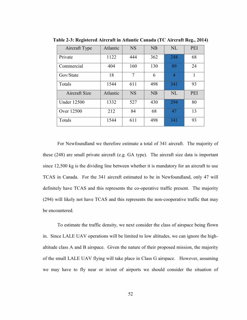
52
Table 2-3: Registered Aircraft in Atlantic Canada (TC Aircraft Reg., 2014)
Aircraft Type Atlantic NS NB NL PEI
Private 1122 444 362 248 68
Commercial 404 160 130 89 24
Gov/State 18 7 6 4 1
Totals 1544 611 498 341 93
Aircraft Size Atlantic NS NB NL PEI
Under 12500 1332 527 430 294 80
Over 12500 212 84 68 47 13
Totals 1544 611 498 341 93
For Newfoundland we therefore estimate a total of 341 aircraft. The majority of
these (248) are small private aircraft (e.g. GA type). The aircraft size data is important
since 12,500 kg is the dividing line between whether it is mandatory for an aircraft to use
TCAS in Canada. For the 341 aircraft estimated to be in Newfoundland, only 47 will
definitely have TCAS and this represents the co-operative traffic present. The majority
(294) will likely not have TCAS and this represents the non-cooperative traffic that may
be encountered.
To estimate the traffic density, we next consider the class of airspace being flown
in. Since LALE UAV operations will be limited to low altitudes, we can ignore the high-
altitude class A and B airspace. Given the nature of their proposed mission, the majority
of the small LALE UAV flying will take place in Class G airspace. However, assuming
we may have to fly near or in/out of airports we should consider the situation of
53
controlled airspace. It is worth noting that statistically, the majority of mid-air collisions
have occurred near airports (i.e. in controlled airspace) involving aircraft in the traffic
circuit (TSB, 2012). Class C would represent a situation where we must fly near a major
airport such as St. John’s or Gander. Class D will apply if we must operate near a smaller
airport like Deer Lake. We may therefore calculate the total volumes represented by
these three airspace categories, and based on the traffic density in each, the probability
that the UAV would encounter another aircraft.
(a) Traffic Density in Uncontrolled (G Class) Airspace
For the Class G case, the total Volume (V) of the airspace will be considered as
the wilderness area of Newfoundland (i.e. the Newfoundland island area less Metro areas
as shown in Table 2-1) multiplied by an average altitude (h) of 2200ft (670m) AGL,
which is likely the highest altitude a LALE UAV would use in Class G airspace. To
estimate the number of aircraft that would be flying at any given moment (i.e. the
rate/hour) we must assume an average utilization rate for these aircraft. Since the
majority will be private GA (i.e. amateur/hobbyist aircraft) we shall assume a low usage
rate, likely a few hours every week, or about 8 hr/month. Therefore at any given hour
there would be 341x8 / (24x30) or about 4 low-altitude aircraft airborne somewhere over
the island. The traffic density is therefore very low. To calculate the Penc, we next
consider the exposure caused by the UAV flying for one hour. The UAV will sweep out
a volume as it flies, the diameter of which may be chosen to represent either a collision
(MAC) or a near-miss (NMAC) threat zone. This situation is illustrated in Figure 2-5.

54
Figure 2-5: UAV Traveling in Uncontrolled G Class Airspace over Newfoundland
For collisions, we will assume a threat area 30ft/10m wide (i.e. wingspan of a
typical GA aircraft). For the case of near-miss incidents a threat zone with 500ft/150m
radius is more appropriate. The Penc in G class airspace may then be calculated as:
VtransV
nP
class
enc (2-3)
Where:
n = number of aircraft in the air per hour
Vclass = volume of the airspace zone
Vtrans = the volume “swept” by the UAV as is travels through the airspace each hour.
The estimate for the Penc will be calculated for both the MAC and NMAC case, to permit
comparisons with equivalent manned aviation statistics.
(b) Traffic Density in Controlled (Class C/D) Airspace
We next estimate Penc in the controlled airspace zones. The majority of the NL-
registered aircraft used to calculate the G class traffic density represent only the aircraft
which fly locally. This does not include the regular inter-provincial or international air
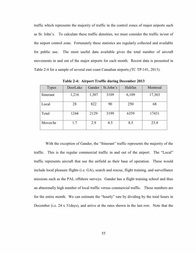
55
traffic which represents the majority of traffic in the control zones of major airports such
as St. John’s. To calculate these traffic densities, we must consider the traffic in/out of
the airport control zone. Fortunately these statistics are regularly collected and available
for public use. The most useful data available gives the total number of aircraft
movements in and out of the major airports for each month. Recent data is presented in
Table 2-4 for a sample of several east coast Canadian airports (TC TP-141, 2013).
Table 2-4: Airport Traffic during December 2013
Types DeerLake Gander St.John’s Halifax Montreal
Itinerant 1,216 1,307 3109 6,109 17,363
Local 28 822 90 250 68
Total 1244 2129 3199 6359 17431
Moves/hr 1.7 2.9 4.3 8.5 23.4
With the exception of Gander, the “Itinerant” traffic represents the majority of the
traffic. This is the regular commercial traffic in and out of the airport. The “Local”
traffic represents aircraft that use the airfield as their base of operation. These would
include local pleasure flights (i.e. GA), search and rescue, flight training, and surveillance
missions such as the PAL offshore surveys. Gander has a flight training school and thus
an abnormally high number of local traffic versus commercial traffic. These numbers are
for the entire month. We can estimate the “hourly” rate by dividing by the total hours in
December (i.e. 24 x 31days), and arrive at the rates shown in the last row. Note that the
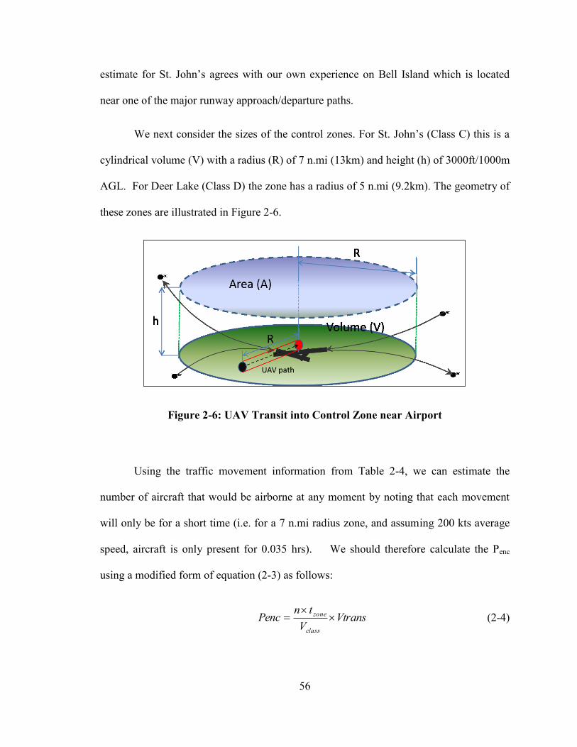
56
estimate for St. John’s agrees with our own experience on Bell Island which is located
near one of the major runway approach/departure paths.
We next consider the sizes of the control zones. For St. John’s (Class C) this is a
cylindrical volume (V) with a radius (R) of 7 n.mi (13km) and height (h) of 3000ft/1000m
AGL. For Deer Lake (Class D) the zone has a radius of 5 n.mi (9.2km). The geometry of
these zones are illustrated in Figure 2-6.
Figure 2-6: UAV Transit into Control Zone near Airport
Using the traffic movement information from Table 2-4, we can estimate the
number of aircraft that would be airborne at any moment by noting that each movement
will only be for a short time (i.e. for a 7 n.mi radius zone, and assuming 200 kts average
speed, aircraft is only present for 0.035 hrs). We should therefore calculate the Penc
using a modified form of equation (2-3) as follows:
VtransV
tnPenc
class
zone
(2-4)
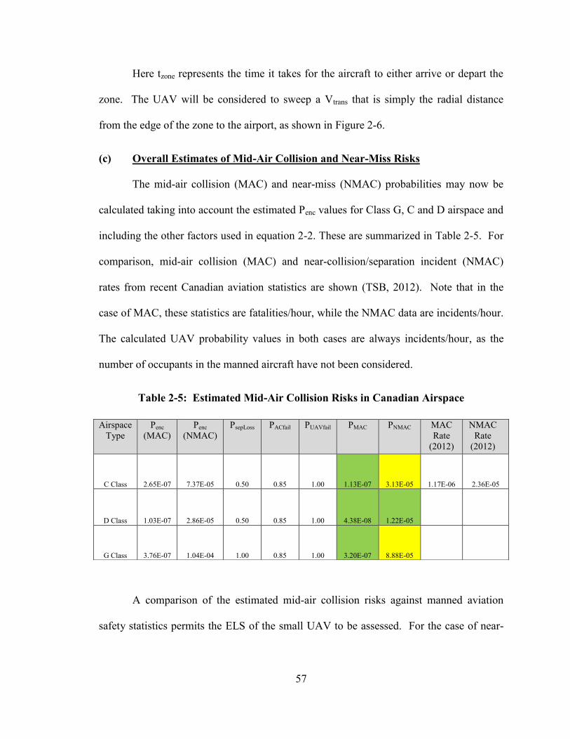
57
Here tzone represents the time it takes for the aircraft to either arrive or depart the
zone. The UAV will be considered to sweep a Vtrans that is simply the radial distance
from the edge of the zone to the airport, as shown in Figure 2-6.
(c) Overall Estimates of Mid-Air Collision and Near-Miss Risks
The mid-air collision (MAC) and near-miss (NMAC) probabilities may now be
calculated taking into account the estimated Penc values for Class G, C and D airspace and
including the other factors used in equation 2-2. These are summarized in Table 2-5. For
comparison, mid-air collision (MAC) and near-collision/separation incident (NMAC)
rates from recent Canadian aviation statistics are shown (TSB, 2012). Note that in the
case of MAC, these statistics are fatalities/hour, while the NMAC data are incidents/hour.
The calculated UAV probability values in both cases are always incidents/hour, as the
number of occupants in the manned aircraft have not been considered.
Table 2-5: Estimated Mid-Air Collision Risks in Canadian Airspace
A comparison of the estimated mid-air collision risks against manned aviation
safety statistics permits the ELS of the small UAV to be assessed. For the case of near-
Airspace
Type
Penc
(MAC)
Penc
(NMAC)
PsepLoss PACfail PUAVfail PMAC PNMAC MAC
Rate
(2012)
NMAC
Rate
(2012)
C Class 2.65E-07 7.37E-05 0.50 0.85 1.00 1.13E-07 3.13E-05 1.17E-06 2.36E-05
D Class 1.03E-07 2.86E-05 0.50 0.85 1.00 4.38E-08 1.22E-05
G Class 3.76E-07 1.04E-04 1.00 0.85 1.00 3.20E-07 8.88E-05
58
miss (NMAC) risk (i.e. loss of separation) the UAV poses a higher risk than manned
aviation in Class C and G airspace. The risk in Class D is estimated to be about half that
of than manned aviation in Canada. The risk in Class C is slight higher (1.3 times). The
risk is about 3.8 times higher for Class G. The lack of any sort of mitigation factors to
prevent traffic conflicts has a detrimental effect on the NMAC safety level, especially in
uncontrolled airspace.
A similar comparison of the PMAC rates against statistical data shows that in all
three airspace situations analyzed, the UAV rate is actually better than the most recent
Canadian manned aviation statistics. However, except for the situation in Class D, the
calculated ELS and statistical results are worse than the target ELS goal of 1e-7. Indeed,
the most recent published Canadian PMAC rate is almost twelve times worse than this
target, due to one particularly costly incident in Saskatchewan in 2012 (TSB Report
A12C0053, 2012).
2.5 Summary: The Current Level of Safety (ELS)
The current estimated levels of safety for the small UAV may now be summarized
as follows9:
2.5.1 Ground Risk
1. Assuming current small UAVs like the Aerosonde can claim an MTBF of 100-
150 hours, it may be considered as safer (or better) than GA aircraft operating in
remote wilderness conditions (e.g. Labrador). The calculated ELS is actually
9 The material in this Chapter plus a discussion of the effects of various mitigation strategies is the subject of a recent Journal of
Unmanned Vehicle System article prepared by the author and his supervisors (Stevenson, O'Young, & Rolland, 2015).
59
two times safer than the equivalent GA accident risk, assuming the worst case
Canadian data from 2012.
2. The same UAV would have to demonstrate at least 2000 hours MTBF to
maintain equivalent safety levels as manned aircraft while flying over more
densely populated rural areas (e.g. island portion of NL). It is doubtful that any
current small UAVs can claim this level of reliability.
3. The small UAV cannot operate over sub-urban or urban areas and claim to be as
safe as even the most basic GA manned aircraft with the current level of
reliability.
2.5.2 Mid-Air Collision Risk
1. In uncontrolled Class G airspace, the small UAV appears to have a NMAC rate
that is about 3.8 times worse than equivalent Canadian statistics. The MAC rate
is better than the most recent (2012) Canadian statistics, but this rate is 3.2 time
worse than the target ELS of 1x10⁻⁷
.
2. In controlled Class C airspace, the small UAV appears to have a slightly higher
NMAC risk (1.3 times) versus manned aircraft. The mid-air (MAC) risk is
lower than the most recent Canadian MAC data, and comparable to the target
ELS.
3. The small UAV does not appear to present an increased collision risk in Class D
airspace, assuming the low traffic concentration used (~2 aircraft/hour) is true.
2.5.3 Where the Small UAV Needs to Improve
It must be the goal of any improvements to the safety of small UAVs to not simply
match manned aviation accident rates, but to exceed them. In order to do this, a number of
deficiencies identified with the small UAV must be corrected. The most serious ones
which have the strongest impact are summarized below:
60
1. Poor Situational Awareness - the small UAV has poor situational awareness,
especially when they are operated at BLOS ranges. The lack of a viable DSA
capability remains the main hurdle preventing integration of the small UAV into
non-segregated airspace. Some means must be found to improve the awareness of
the UAV and also the awareness of the AVO at the GCS.
2. Poor Visibility – the small UAV is essentially invisible to other air space users.
Some means of enhancing its visibility must be found. Note that “visibility” here
includes detectability under both visual (VFR) and instrumentation (IFR) flight
conditions.
3. Poor Reliability - the low quality common in many small UAVs must be
addressed, as these have a direct effect on the need for repairs, excessive
maintenance, and generally results in poor reliability. Only once this is improved
will the small UAV have the demonstrated reliability that would allow greater
freedom to operate over higher density populated areas. Note that an
improvement in reliability would also have the most impact on many of the
Perceived Risks associated with small UAVs in the current political climate.
4. Manual Operations – the previous deficiencies affect the real physical risks
calculated. However, Manual Operations (Control) must be considered as another
source of lowered reliability of the small UAV, and a great concern to operators
and regulators, especially in terms of financial and crew risk. The excessive use
of manual R/C piloting methods increases the risk of a landing or take-off mishap,
especially for the higher-performance small UAVs. A paradigm shift is required
to operate these airframes using higher levels of automation and improved control
methods, especially if the small UAV is to be used in expanded roles and in all
weather conditions.
2.5.4 Mitigation Strategies
It is clear that developing a viable DSA system remains a major goal for civilian
UAV operations. There are hopeful signs that a limited capability may be possible in the

61
near future based on ADS-B transponders. However, even before this DSA capability is
realized, there may be methods we could use now to improve the safety of the small
UAV. Research into these mitigation strategies will be discussed in the following
chapters of this thesis.
1. Improving Control - It is proposed that novel methods can be used to
improve the reliability and controllability of the small UAV, especially during
take-off and landings. A novel Beyond Line of Sight (BLOS) control method
using a synthetic environment approach may also be possible. Chapter 3 will
focus on these subjects.
2. Improving Visibility – a number of techniques used in manned aviation may
be applicable to the small UAV. Chapter 4 will focus on how these may be
applicable (or not). The potential methods include using transponders to
improve IFR visibility and anti-collision lights for VFR visibility. Giving the
UAV some form of air-to-air radio (communication) capability will also be
explored.
3. Improved Avoidance Methods – an improved avoidance method will be
proposed as the “reaction” portion of a hypothetical DSA capability. A
simulation method and initial work into a promising collision avoidance
method based on an Anti-Proportional Navigation guidance law will be
detailed in Chapter 5.
62
Chapter 3 UAV Control and Situational Awareness
Since 2005 this author has been involved in researching technologies and
operational methods with the aim to improve the reliability and safety of small UAVs
when under manual control. This chapter will provide a summary of the results from
these efforts. Improvements may be possible in terms of improved control accuracy and
enhanced situational awareness, resulting in improved safety. The primary objective is to
mitigate the Ground Impact risk. Improved situational awareness may also reduce some
of the Mid-Air collision risk from UAV operations.
3.1 Introduction to UAV Control Methods
If we survey the current situation with UAVs ranging from the small UAV up to
the larger military types, we find that similar control methods are common throughout.
The most common methods, grouped into Autonomous or Manual Control modes are:
1. Autonomous Control:
a. GPS-based Autopilot (AP) control using waypoints to define a flight plan;
b. Inertial, airspeed and pressure sensors used for attitude, airspeed and altitude
control (i.e. inner-loop airframe control); and,
c. Automatic Take-off and Landing (ATOL) capabilities offered by some autopilots,
using D-GPS and high-resolution altimeter sensors and/or external ATOL system
installed at airfield.
2. Manual Control:
a. Radio Control (R/C) Aircraft methods by an External Pilot (EP) using un-aided
third person visual view of the remote UAV, very common with small UAVs;

63
b. A Flight Console, similar to a dual-pilot cockpit, using a forward fixed camera
view to allow a Manual Pilot (MP) to fly the UAV as in a simulator. This mode is
especially popular with military UAVs like the Predator; and,
c. Virtual Reality (VR) methods employing various forms of FPV flying. This is
becoming increasingly popular in the R/C hobby as an alternative to the traditional
remote third-person view.
While it is true that some autopilots provide a capability to conduct Automatic
Takeoff and Landings (ATOL) it is the experience of our research team as well as the
majority of small UAV operators in North America, that manual control methods are
more common with small UAVs. This is in spite of the fact that a careful review of
available UAV accident reports reveals that the majority of UAV accidents occur during
take-off and landing, especially by UAVs which rely on a manual pilot to accomplish
these tasks (Williams, 2004). In the EP-dependant systems takeoff and especially landing
errors account for a majority (68% to 78%) of the accidents. For the other UAVs the
causes for accidents appeared to be more or less evenly split between equipment failures
and air crew procedural errors. There were human-factor relate problems noted due to
GCS display designs especially with the Predator GCS at that time (Williams, 2004).
This later finding is very interesting when the crash of a Predator-B in Nogales, Arizona
is considered; as that incident was primarily caused by a controls settings error that was
traced to the GCS design (NTSB/CHI06MA121, 2006).
In our experience, the reason why ATOL is avoided in small UAVs is the
difficulty in obtaining a reliable control system especially with small airframes, given the
limited accuracy of most low-cost autopilots, which results in poor-quality (and at times

64
hazardous) automated landings. In most cases, it is deemed much easier and safer to
have a highly-skilled EP conduct the takeoffs and landings. A similar reluctance to use
ATOL is evident in larger military UAVs such as the Predator. The Predator requires that
a highly-trained UAV pilot conduct the landings and takeoff at a forward GCS, before
passing off autonomous control to a remote GCS which might be located on the other side
of the world (Hodges, 2009). This concept of operations (CONOPS) is still the normal
mode for operational Predators, despite recent demonstrations of enhanced ATOL
capabilities (ASDNews, 2012).
Therefore, for a typical small UAV, the mission will most likely progress through
these flight stages:
1. Takeoff (Manual Control)
2. Transition to Automatic Control
3. Autonomous Flight (AP in control)
4. Transition back to Manual Control
5. Landing
The External Pilot (EP) will conduct the take-off manually and climb to a pre-
selected altitude and establish a stable loiter circuit over the launch site (Stage 1). Once
airborne and at a stable altitude and flight condition, control will be switched to
autonomous control (Stage 2). Once stable AP control is confirmed (though with the EP
vigilant and prepared to regain manual control should there be a problem), the UAV will
now fly its mission relying on an on-board autopilot (AP), with supervisory control by an
AVO located at the Ground Control Station (Stage 3). At the conclusion of the mission,
65
the UAV will fly to its recovery airbase, and once in visual range and ready to land,
control will be switched back to manual control (Stage 4). The EP will now resume
control of the UAV and land it manually (Stage 5).
It should be noted that even if a fully-autonomous UAV control capability were
provided (i.e. including ATOL) there will still be a requirement for a manual “safety
pilot” according to current and proposed UAV operating guidelines. There is the
requirement that a competent UAV pilot shall be available and ready to assume control of
the aircraft during all stages of flight, especially in the event of a failure in the autopilot or
if an unsafe situation develops. All SFOCs obtained to date by this research team have
required the presence of such a “safety pilot” for each and every UAV that is airborne
(TC SI-623-001, 2014). Similar rules and regulations are under development in both the
U.S. (FAA, 2008) and Europe (European Commission, 2009).
It must also be recognized that providing a manual override capability at all stages
of UAV operations is a challenge, especially when operations at Beyond Line of Sight
(BLOS) ranges or in non-visual flying conditions are considered. For example, if basic
R/C methods employing unassisted third-person flying techniques are used, effective
manual control is limited to at most 1 km and only under benign daytime visual weather
conditions. Manual override control at BLOS ranges or in non-visual conditions is
currently not possible using standard manual UAV control methods now employed by
most small UAVs. This lack of a viable BLOS manual control method is cited as one of
the major limitations to the legal operational range of small UAVs in the current
regulatory environment, the other being the lack of a reliable DSA system (Ellis,
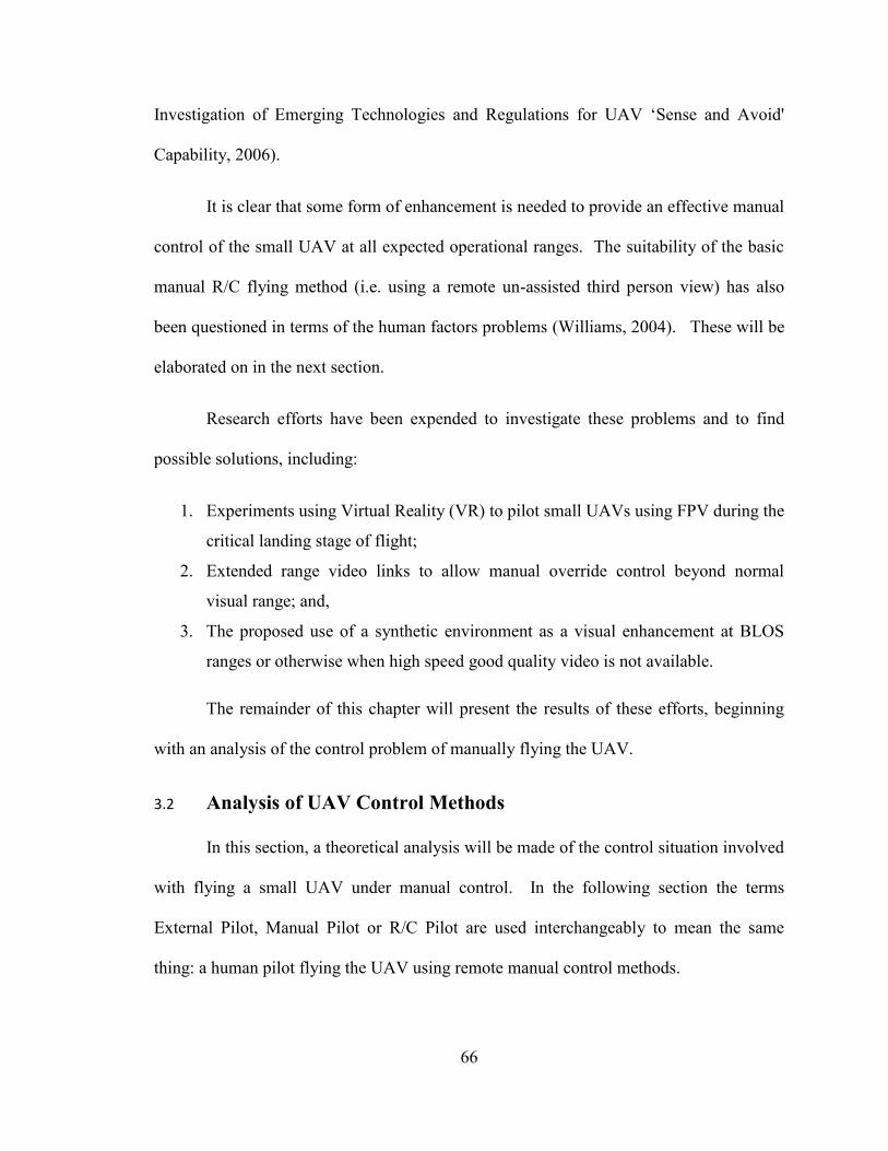
66
Investigation of Emerging Technologies and Regulations for UAV ‘Sense and Avoid'
Capability, 2006).
It is clear that some form of enhancement is needed to provide an effective manual
control of the small UAV at all expected operational ranges. The suitability of the basic
manual R/C flying method (i.e. using a remote un-assisted third person view) has also
been questioned in terms of the human factors problems (Williams, 2004). These will be
elaborated on in the next section.
Research efforts have been expended to investigate these problems and to find
possible solutions, including:
1. Experiments using Virtual Reality (VR) to pilot small UAVs using FPV during the
critical landing stage of flight;
2. Extended range video links to allow manual override control beyond normal
visual range; and,
3. The proposed use of a synthetic environment as a visual enhancement at BLOS
ranges or otherwise when high speed good quality video is not available.
The remainder of this chapter will present the results of these efforts, beginning
with an analysis of the control problem of manually flying the UAV.
3.2 Analysis of UAV Control Methods
In this section, a theoretical analysis will be made of the control situation involved
with flying a small UAV under manual control. In the following section the terms
External Pilot, Manual Pilot or R/C Pilot are used interchangeably to mean the same
thing: a human pilot flying the UAV using remote manual control methods.
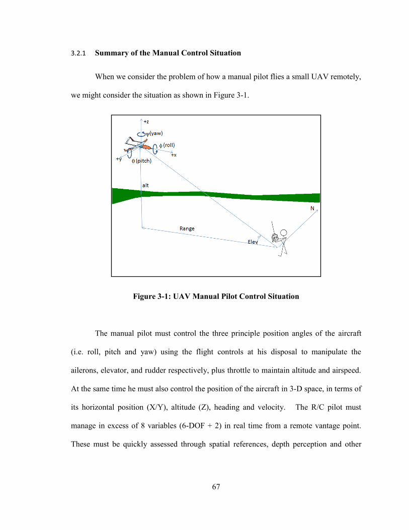
67
3.2.1 Summary of the Manual Control Situation
When we consider the problem of how a manual pilot flies a small UAV remotely,
we might consider the situation as shown in Figure 3-1.
Figure 3-1: UAV Manual Pilot Control Situation
The manual pilot must control the three principle position angles of the aircraft
(i.e. roll, pitch and yaw) using the flight controls at his disposal to manipulate the
ailerons, elevator, and rudder respectively, plus throttle to maintain altitude and airspeed.
At the same time he must also control the position of the aircraft in 3-D space, in terms of
its horizontal position (X/Y), altitude (Z), heading and velocity. The R/C pilot must
manage in excess of 8 variables (6-DOF + 2) in real time from a remote vantage point.
These must be quickly assessed through spatial references, depth perception and other
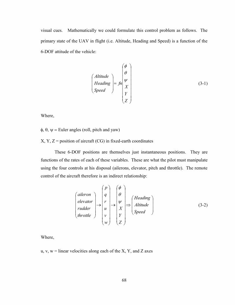
68
visual cues. Mathematically we could formulate this control problem as follows. The
primary state of the UAV in flight (i.e. Altitude, Heading and Speed) is a function of the
6-DOF attitude of the vehicle:
Z
Y
Xfn
Speed
Heading
Altitude
(3-1)
Where,
Euler angles (roll, pitch and yaw)
X, Y, Z = position of aircraft (CG) in fixed-earth coordinates
These 6-DOF positions are themselves just instantaneous positions. They are
functions of the rates of each of these variables. These are what the pilot must manipulate
using the four controls at his disposal (ailerons, elevator, pitch and throttle). The remote
control of the aircraft therefore is an indirect relationship:
Speed
Altitude
Heading
Z
Y
X
w
v
u
r
q
p
throttle
rudder
elevator
aileron
(3-2)
Where,
u, v, w = linear velocities along each of the X, Y, and Z axes

69
p, q, r = angular rates for each Euler angle (roll, pitch, yaw)
This control must be accomplished in real-time, quickly yet smoothly, to maintain
good positive control of the UAV. If we add the extra problem of spatial disorientation
caused by the aircraft being in a strange attitude (e.g. upside down, pointing straight up,
etc.), or the control reversal phenomenon when the aircraft is flying towards you, the
difficulty of the manual pilot problem becomes clear. More than a few R/C aircraft have
been destroyed by this control reversal phenomenon, especially due to incorrect rudder or
aileron control inputs. There is also the problem of what happens if the aircraft flies too
far away, too high, or in difficult lighting conditions (e.g. into bright sun, silhouetted
against clouds, etc.). This can make it difficult if not impossible to determine the UAV’s
orientation, which in turn leads to incorrect control inputs and the risk of going out of
control.
3.2.2 First Person versus Third Person View
If the manual pilot switches from an external third person view to FPV several
things happen. The control of the pitch, roll and yaw of the aircraft are now directly
connected to the pilot’s forward view. In a sense, the aircraft becomes an extension of his
or her body. The need to do the rapid assessment of orientation using an external view is
eliminated altogether. The pilot can now focus on the key parameters of flight which any
full-sized pilot must master – maintaining heading, altitude and airspeed. The control of
pitch, roll and yaw become more or less instinctual. The control problem is reduced by at
least three variables, and perhaps as much as six. The pilot also does not need to figure

70
what each individual component of the 6-DOF position assuming the FPV provides an
accurate indication of the poise of the aircraft (i.e. through a good artificial horizon and
forward video display). What is more important is to maintain heading, altitude, and
speed - and from these the XYZ position follows.
An analogy may be the arguably easier task of driving a car. With the removal of
the need to manage the third axis (i.e. up/down), the task of driving becomes one of
steering the vehicle in the right direction and managing the speed properly. But, as
anyone who has ever tried to drive one of those small R/C cars can attest, this task
becomes much more difficult when we are forced to use a third person remote view. If
real vehicles were as difficult to drive as the R/C car experience would suggest, cars
should be leaving the sides of roads every 200-300 m along their intended journey!
Clearly, being inside the vehicle with a good forward view appears to simplify the manual
control problem and improves accuracy.
A summary of the human factors problems associated with using remote third-
person R/C control of a small UAV is provided in Table 3-1. As noted this is a
combination of the conclusions determined in previous reports (Williams, 2004) and the
analysis by this author (Stevenson, O'Young, & Rolland, 2015).
71
Table 3-1: Human Factor Problems with Manual R/C Control Methods
Human Factor Problem Source
Control reversal/disorientation Williams/Stevenson
Visual problems (bad lighting/aircraft
orientation)
Stevenson
Limited range (< 500m) Stevenson
Limited to VMC conditions Williams/Stevenson
Airframe dynamics too fast Stevenson
Training Problem (limited external pilot skillset
availability)
Williams/Stevenson
The incorporation of the FPV view should improve the controllability of the
airframe. However, it must be recognized this benefit only applies if the manual pilot is
already familiar with manned flight, and knows the basics of good airmanship. Of course
the dynamics of the small UAV and any control delays must also be considered, as will be
discussed in the next section.
3.2.3 The Problem of Control Delays
The problem of flying a small UAV using manual methods is closely linked to the
dynamics of the airframe being controlled and any control delays that are imposed. If
these delays or the aircraft dynamics become extreme, accurate manual control becomes
difficult if not impossible. An analysis can be done to quantify the sources of delay that
contribute to the control lapse rate situation during remote manual piloting. Three
different methods for manually piloting are shown schematically in Figure 3-2, with
annotations showing the sources of the delays.

72
Figure 3-2: Sources of Control Delay during Manual Piloting
The total control lag will vary considerably depending on the form of remote
manual control used. Taking a simple view, the total lag will be the sum of all of the sub-
element delays. In the worst case scenario, it would be:
delay = pilot + a/c comm + gcs (3-3)
Where each term is described below:
a) pilot = Human Operator (pilot) Reaction Time
A major contributor to the manual control lag is the reaction time of the pilot.
Typical human reaction times to simple stimuli have been measured and range from 150
to 300 ms, with 250 ms being typical for alert operators. Age, environmental conditions

73
(e.g. light level), fatigue and general situational awareness are factors in determining the
reaction time of a specific person. Highly trained individuals such as athletes and pilots
can condition themselves to improve this reaction time, although consistently the best
reaction time is on average 180 ms (McCormick, 1970). Note that these are reaction
times to expected events (e.g. such as during normal closed-loop control of an aircraft).
Reactions to unplanned or unexpected events can be much slower. The average reaction
time in this situation is commonly quoted in the literature as 750 ms (e.g. this is typically
used for estimating automobile stopping distances). However, this figure has been called
into question by some, as it is also based on clinical testing. In independent tests of
drivers in realistic situations, reaction times of up to 2 seconds were measured for entirely
unexpected and unplanned events (Lerner, 1993). Given the relatively predicable nature
of R/C control, a value of 250 ms will be assumed for normal closed-loop control of a
small UAV.
b) a/c = Response Lag of the Airframe (i.e. especially roll or pitch rates)
This term is dominated by the aerodynamics of the airframe and also the avionics
response rates (i.e. servos and flight surfaces). For the size of vehicle being considered
here, the dynamic response of the avionics/servos are very fast for hand-flown UAVs,
typically about 20 Hz, equivalent to a lag time of about 5 ms (Barnard, 2007).
c) comm = Communication Lag (Video and Telemetry)
This is the combination of processing delays in the communication hardware plus
the physics involved in radio frequency (RF) signal transmission (i.e. speed of light
74
propagation) in both the send and receive directions. The magnitude of this total delay
varies considerably depending on the form of control being used. For the case of a
Manual Pilot (1) standing by the runway, or a Virtual Pilot sitting at a local GCS (2), the
major source would be delays in the video/data feeds, perhaps due to hardware limitations
in the RF link, or any delays in sending the manual control inputs back to the UAV. The
total RF signal transmission path itself is insignificant (i.e. less than 2 km round trip),
resulting in total transmission delays of under 7 microseconds. Limitations in RF
transmission rates (especially for small video cameras) were an issue in the past, however
even small low-end video cameras are now common and can transmit TV-quality (at least
25 Hz frame rate, typically as high as 60 Hz) video over a range of up to 6 km. Transfer
of airframe data (i.e. data to drive a virtual cockpit display or Heads-Up Display/HUD)
and the manual control signals back to the airframe must be kept at a rate to match the
video update rate to ensure synchronization between the video and the aircraft attitude.
The situation changes when attempting to tele-operate the UAV from a remote
GCS as in (3). In this case, the communication lags could become very significant. This
is particularly true if the communication channel makes use of communication satellites.
Turn-around delays of at least 500 ms and as much as 7 seconds are noted by some UAV
researchers, especially if geostationary types are used (Clough, 2005). If a terrestrial feed
is used (e.g. through an internet connection – the horizontal path from the local
GCS/receiving station to a remote GCS as shown in Figure 3-2 the channel delays would
be dictated by the overall capacity of the network connection. The speed of the “weakest
link” would determine the maximum throughput. This is likely to be the first link, from
75
the local GCS which will typically be in a remote location and most likely away from
high capacity hard-wired communication cables. In this case a wireless internet link to a
nearby community or repeater tower may impose serious restrictions on the maximum
data rate, possibly as low as 56Kbit/sec. This may be adequate for attitude/control data
but would severely limit the quality and frame rate of the video signal provided to the
manual pilot.
d) gcs = Delays in GCS Console (Software and Hardware)
Delays in the computer console itself (i.e. GCS computer software or hardware)
may contribute to the control latency. This is not as great a concern as it was over a
decade ago. For example, most current laptop PCs are capable of running graphics-
intensive software (i.e. games or flight simulators) while maintaining an animation frame
rate well above the “flicker limit” of 25 Hz. Frame-rates of 50-60 Hz are common. To be
prudent we will assume 25 Hz as worst case here.
Assuming reasonable values for each delay term, the overall control delay for each
of the three Virtual Pilot (VP) scenarios may be calculated:
(1) Manual Pilot: delay = delay = pilot + a/c = 250 + 5 = 255 ms
(2) Local GCS: delay = pilot + a/c + gcs = 255 + 1/25 = 359 ms
(3) Remote GCS: delay = pilot + a/c comm + gcs = 359 + 500 = 859 ms (best case)
to 7.6 sec (worst case)

76
3.2.3.1 Comparison with Typical UAV Airframe Dynamics
Stable control of the UAV can only be assured if the overall speed of the
controller (i.e. Manual Pilot including delays) is faster than the airframe. As a rule of
thumb, it is desirable for the controller to be several times faster than the plant (i.e.
airframe) under control, ideally ten times faster although five times is acceptable
(Mohammed S. Santina, 1996). Therefore for the local Manual Pilot (Case 1) we can
estimate that the aircraft being controlled should have a minimum time constant of around
1.3 sec. The corresponding “controllable” airframe is slightly slower (1.8 sec) for the
Local GCS (Case 2), but quite a bit slower (4.3 sec) for the Remote GCS (Case 3) even
for the best-case communication scenario.
This analysis confirms what this author has observed during operations of the
Aerosonde UAV and the GiantStik while under Manual Pilot control. Landing speeds
(and dynamics) are relatively benign for the GiantStik. It lands with full flaps at about 8
m/s (~29 km/hr) with the engine still operating. The overall airframe response time in
roll in good weather is something like 1.5-2.0 seconds. Therefore while fast, the
GiantStik should still be within the control ability of most intermediate R/C pilots. In
contrast, the Aerosonde lands typically at 18 m/s (~65 km/hr) without engine power. Its
longitudinal (roll) axis time constant is estimated to be 0.75-1.0 seconds. This is below
the range where a typical human operator can maintain control, and is why highly-skilled
R/C pilots are needed for the Aerosonde EP role.
77
The combination of a fast airframe and excessive control delays may make it
fundamentally impossible to safely control the small UAV under manual control. During
Aerosonde UAV trials, our EP noted a small lag (about 0.25 sec) when moving the
Aerosonde flight surfaces using a standard R/C console, but with the control signals
processed and transmitted by the Piccolo GCS. He noted that this lag was not present
when flying his own normal high-performance R/C aircraft using direct R/C control
(Trickett, 2007). The sensitivity of the Aerosonde UAV, especially in roll, was always a
cause for concern. The additional lag identified by the EP may have been a major
contributor to the crash of the second Aerosonde Trainer (AC171) on 8 June 2008 at Bell
Island. If we compare the roll rate of the Aerosonde with the control lag of an EP whose
commands must pass through a GCS (i.e. Case 2) that imposes an additional 0.25 sec
delay, we see that the safe control of the Aerosonde under manual control is questionable,
especially at critical times such as when flying very close to the ground.
3.3 Virtual Reality Pilot Experiments
3.3.1 Various Manual Piloting Methods
There are several possible forms of manual control that might be used to control a
small UAV. A Virtual Pilot view (i.e. FPV10
equivalent to a manned aircraft cockpit
view) is hypothesized to be one way where the controllability of small UAVs may be
improved during the most crucial portions of a mission - the takeoff and landing of the
10 At the time of the planning and implementation first set of experiments documented here (i.e. 2006-2010) the accepted
terminology for this technology was called Virtual Reality (VR). However, in the years since that time, and with the increased
availability of such equipment in the R/C hobby, First Person View (FPV) has become the more popular description of these methods. This is in contrast to the remote third person view normally used for R/C flying. In the following text both terms will be used
interchangeably.
78
aircraft. This is a common technique used with larger military UAVs such as the
Predator, which has become possible in smaller vehicles due to availability of
miniaturized Virtual Reality (VR) equipment at reasonable cost.
A series of experiments have been conducted to answer the question: “What form
of virtual (manual) piloting is the best method, or the most appropriate for small UAVs?”
Three different forms of UAV manual control were assessed:
(a) Radio Control (RC) Mode - the current “default” method, whereby the UAV
autopilot is overridden and the aircraft is flown using standard Radio Control
(R/C) techniques, using an un-aided external third-person view of the aircraft.
(b) Flight Simulator (FS) Mode - A fixed forward camera view along the aircraft
centerline, providing a FPV to the pilot on a fixed screen in front of him. The pilot
therefore flies the UAV in a manner similar to a flight simulator. Ideally, the pilot
should be sitting down and use a joystick, similar to modern fly-by-wire cockpits.
(c) Immersive (VR) Mode – A fully immersive view using VR Goggles, providing a
FPV binocular video image on a set of tiny LCD screens directly in front of both
eyes of the pilot. These goggles also featured 2-axis tilt sensors on the “forehead”
of the goggle housing, providing a head-tracking ability. This allowed the VR
pilots to turn his head and pan/tilt the camera on the aircraft, giving the illusion of
being on the aircraft.
This may be the first time that this sort of objective experimental method has been
used to assess VR methods on small UAVs, apart from attempts to establish VR training
systems for UAVs (Smith & Smith, 2000). This experiment focused on the critical
Landing phase to allow an assessment of maneuver accuracy while using these three
different control methods.

79
3.3.2 The VR Landing Experiment Design
The VR experiment used a Design of Experiments (DOE) factorial approach.
This allows the use of a sparse matrix of test factor combinations while preserving the
statistical validity of the results. This is useful when conducting real-world tests where
running a full statistical set of all possible combinations would be too expensive,
dangerous or impractical. The objective in the DOE method is to determine those factors
which are the most significant to the response variables being studied. By using a
randomized order of test runs, the effect of random factors beyond the researchers’
control is minimized and appears as “noise” in the statistical analysis.
Figure 3-3: Diagram of Landing Task Used for VR Experiment
Figure 3-3 illustrates the task used as the basis for this experiment – landing a
small aircraft (UAV) under manual control on a small runway of fixed heading. The goal
during these experiments was to assess the relative “quality” of each landing. The

80
primary objective is to land the UAV on the centerline of the runway, preferably just past
the near end of the runway. This allows room for a successful post-landing roll out and
deceleration without running off the far end of the runway. At the same time, the track
should be straight down the center of the runway, to avoid violent lateral accelerations
and to avoid sideways runway excursions.
3.3.2.1 Factors Considered (Independent Variables):
The following factors were studied in this experiment:
A = Form of Manual Piloting:
Radio Controlled (RC) mode (i.e. 3rd
person view of aircraft)
Flight Simulator (FS) mode (FPV using fixed forward display on a screen)
Immersive (VR) Mode (FPV using VR Goggles with head tracking)
B = Skill Level of Pilot
Veteran (10+ years’ experience)
Rookie (<2 years’ experience)
C = Wind Conditions
Calm (<10 km/hr)
Windy (>30 km/hr)
3.3.2.2 Response Variables
To assess the quality of each landing, the following Response Variables were used:
X = Distance of landing touchdown point from landing end of runway
81
Y = Maximum deviation of landing track versus runway centerline. During the
experiment it was noted this was the touch-down point, as both pilots corrected quickly to
the centerline once landed.
3.3.3 Argentia VR Landing Experiment (2010)
The originally proposed test location was the Bell Island Airstrip (CCV4). This is
a single 2700 x 66 foot runway with heading 26-08, located on Bell Island in the middle
of Conception Bay, Newfoundland. However, due to demonstrated concerns on previous
UAV missions with the security of the site, the test location was moved to the abandoned
U.S. Air Base at Argentia, Newfoundland. Although much of the original runway and
tarmac pavement has deteriorated over the decades, there is still a substantial area that
was found to be adequate for small UAV testing. One such area was a taxiway for
strategic bombers (SAC). In an attempt to establish an equivalent situation as on Bell
Island, a section of pavement was marked with high-visibility (green) spray paint,
establishing a mock-up runway 8m wide by 80m long. This runway and the locations of
the mobile GCS, test pilots and video recording cameras are annotated in Figure 3-4. It
was noted by both pilots these were far from aviation-grade runway markings both in
colour and size, and difficult to see from the air. However, the centerline of the marked
runway did correspond to the centerline of the taxiway. Even after 30 years the centerline
marking was still visible. The large green target in the center of the hand-drawn runway
could also be seen during final approach. Thus, while not ideal, the test setup was
deemed adequate for the basic assessment of landing accuracy.

82
Figure 3-4: Test Site at Argentia (2010)
3.3.3.1 Flight Test Vehicle
A large R/C aircraft was used as the test vehicle. In 2010, the Great Planes “Giant
BigStik” (hereafter called the GiantStik) was the largest member of this family of R/C
aircraft, with a wingspan of 80”, and nominal gross weight of 13-15 lbs. A detailed
description is given in Appendix D. This test vehicle is shown with the author in Figure
3-5. The GiantStik uses a symmetric airfoil which has favourable handling properties,
especially in the high winds common to Newfoundland. Originally, a gasoline-powered
version of the GiantStik was planned, but was converted to electric power. This reduced

83
the vibration issues previously encountered during initial tests of the VR equipment, and
provided a stable video image for the pilots.
Figure 3-5: GiantStik Test Vehicle
3.3.3.2 The Pilots of the 2010 Experiment
For the 2010 VR Experiment, two pilots were recruited from the Project RAVEN
team to act as the test pilots. The two pilots used were:
a) Marc Schwarzbach (the “veteran”), a German graduate student who spent
2010-2011 flying with Project RAVEN as the primary manual pilot. At the time
Marc had approximate 10 years’ experience flying R/C aircraft (mostly electric
types) in Europe. He was also very familiar (and enthusiastic) about the use of
VR flying methods, having tried it himself on several occasions in Germany.
b) Jesse Ross-Jones (the “rookie”), one of the local graduate students who joined
Project RAVEN in 2009. A recent flyer, he had only achieved his “wings” earlier

84
in the Summer of 2010. However, he was very comfortable flying the electric
GiantStik and thus was an ideal “rookie” flyer candidate.
3.3.3.3 2010 VR Equipment
Figure 3-6 provides a schematic of the VR equipment setup that was used during
the 2010 VR Landing experiment. As shown, the equipment may be divided into a set of
Airborne and Ground Components.
Figure 3-6: VR Equipment Schematic (2010)
I. Airborne Components:
a) Camera and Turret in 4” Dome - The onboard camera was mounted on a 2-axis
turret inside a small 4” acrylic hemispheric dome assembly. This assembly was

85
mounted to an aluminum flashing belt which provided the anchoring method to
the aircraft, using the existing main wing attachment bolts and dowels. Figure 3-7
shows a close-up of the VR Dome assembly installed on the test vehicle.
Figure 3-7: VR Dome Installation (2010)
The camera and turret were obtained as part of the X11 FPV VR Set from RC-
Tech in Switzerland in 2007 (RC-Tech, 2010). The video image was provided by a small
NTSC-format camera with a 2.4 GHz analog transmitter integrated to the back of the
camera. The power source was a 7.4V 2-cell LiPo battery installed in the cylindrical base
of the turret assembly. The camera and integrated transmitter provided a reasonably clear
image to a maximum range of about 1 km, adequate for the landing experiment, provided
that a tracking 4” x 4” patch antenna was used at the receiver. The use of an analog 2.4
GHz video link meant 2.4 GHz R/C control could not be used, due to severe interference
at the receiver station. For this reason the GiantStik was reverted to 72 MHz FM R/C
86
control. The two-axis turret permitted head-tracking by the camera, using two auxiliary
channels of the aircraft R/C receiver.
b) Azimuth (AZ) Range Extender - for the azimuth (yaw) direction, the range of
the servo was increased to approximately +/- 90º by use of a Pulse Width
Modulation range-doubler. This small unit was installed similar to a servo
extension cable on the AZ servo cable. The increased AZ range allowed the VR
pilot to look over each wing tip, similar to full-size pilot practice.
II. Ground Components:
a) 2.4 GHz AV Receiver - The receive station for the VR video was a small 2.4 GHz
analog receiver, using a 4”x4” patch antenna. During the experiment, the aircraft
was tracked manually by pointing the face of the patch antenna at the vehicle.
This permitted clear video during most of the circuits used during the VR flights.
b) Video Splitter - A video-splitter was used so that the video feed could be sent to
both the VR Goggles and a video capture card on a laptop. Airborne video could
therefore always be seen and recorded, provided a good quality video link was
maintained. Extension cables were used to allow the VR goggles to be worn by
the pilot at a comfortable distance from the receive station.
c) Video Capture Card and Laptop – To permit the video to be displayed and
recorded, a PCMCIA card-bus video capture card was used. The software
provided with the capture card was used to display the VR camera image on
screen, add annotations, and create digital video recordings for each experimental
run. These video clips were recorded for all tests, whether using VR mode or not.
The Laptop screen display was used as the fixed view for the FS mode. This fixed
view corresponded to the mechanical and R/C center of the 2-axis turret, adjusted
to give a view straight along the propeller centerline, and slightly downward
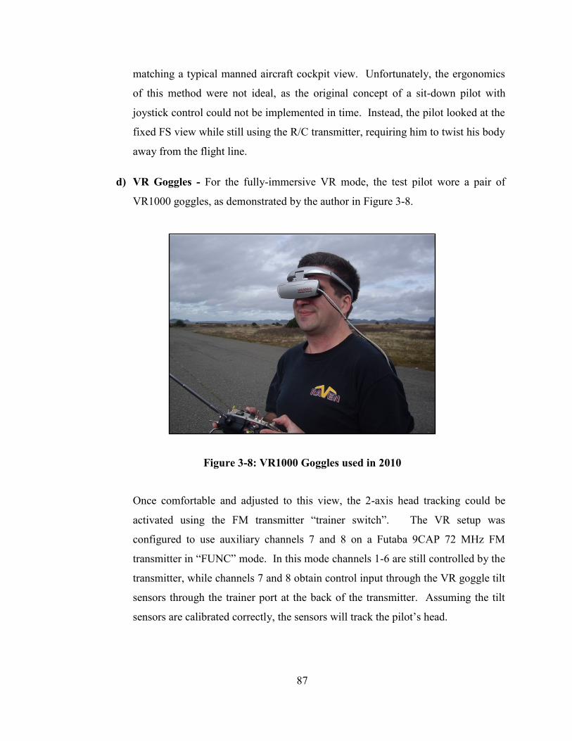
87
matching a typical manned aircraft cockpit view. Unfortunately, the ergonomics
of this method were not ideal, as the original concept of a sit-down pilot with
joystick control could not be implemented in time. Instead, the pilot looked at the
fixed FS view while still using the R/C transmitter, requiring him to twist his body
away from the flight line.
d) VR Goggles - For the fully-immersive VR mode, the test pilot wore a pair of
VR1000 goggles, as demonstrated by the author in Figure 3-8.
Figure 3-8: VR1000 Goggles used in 2010
Once comfortable and adjusted to this view, the 2-axis head tracking could be
activated using the FM transmitter “trainer switch”. The VR setup was
configured to use auxiliary channels 7 and 8 on a Futaba 9CAP 72 MHz FM
transmitter in “FUNC” mode. In this mode channels 1-6 are still controlled by the
transmitter, while channels 7 and 8 obtain control input through the VR goggle tilt
sensors through the trainer port at the back of the transmitter. Assuming the tilt
sensors are calibrated correctly, the sensors will track the pilot’s head.

88
In practical use, the 2-axis tilt sensors were quite sensitive to the way they were
calibrated. A critical step was to leave the goggles motionless on a firm surface during
initial transmitter power-up. The tilt sensors obtain their power through the trainer port
connection. The VR Goggles were left in this position for a period of at least 1 minute.
This allowed the solid-state tilt sensors to properly warm up before attempting to use
them to measure head tracking. Even with careful calibration, it was noted that the head
tracking tended to drift slowly, especially in the elevation direction. A reset button was
provided which re-centered the view to the mechanical center of the airborne turret.
During the VR experiment this was shown to be a minor nuisance, since the pilot would
simply turn his head more to compensate. It was only when the drift moved close to a
mechanical stop that a reset was needed, approximately once every 60 sec.
III. Recording Instruments
In addition to the laptop computer which recorded the onboard video from the VR
camera, two tripod-mounted video cameras were used to record the landings from a side-
runway and end-runway view. The location of the end-view video camera was moved to
the upwind (departure) end of the runway. While the original intent was to use this video
to measure the touchdown points of each landing, it was quicker and more straightforward
to simply note the touchdown point for each landing, and mark the location quickly as
soon as the aircraft had cleared, using sidewalk chalk. Accurate measurements were done
once several landing test points were finished using a surveyors tape. During the

89
experiment, the direction and magnitude of the wind speed was noted, making use of a
mast-mounted anemometer on the mobile GCS.
3.3.3.4 2010 Experimental Results
The experiment was run over two days, August 25-26, 2010. Originally, it was
hoped to run a blend of windy and calm conditions on each day, since this was a factor in
the experiment and thus should have been randomized. However, as is usual for
Newfoundland, the weather did not cooperate. Instead, the runs were divided into two
Blocks, one for each day. The Windy cases were done on Day 1, and are summarized in
Table 3-2.
Table 3-2: 2010 VR Experiment First Day of Tests (Windy Day)
Run Factor A:
Form of VR
Factor B:
Pilot Skill
Factor C:
Winds
Response X:
Touchdown
Location (m)
Response Y:
Centerline
Deviation (m)
1 None/RC Veteran Windy -1.6 +0.75
2 VR Goggles Rookie Windy +2.7 -1.9
3 FlightSim Rookie Windy -2.2 -3.1
4 FlightSim Veteran Windy -42.7 -0.9
5 VR Goggles Veteran Windy -26.3 -0.9
6 None/RC Rookie Windy -2.2 -1.0
7 VR Goggles Rookie Windy +3.7 -1.7
8 None/RC Veteran Windy +3.75 +0.3
9 FlightSim Veteran Windy -24.3 -2.2
10 VR Goggles Veteran Windy -55 -3.5
11 None/RC Rookie Windy -20.4 -0.3
12 FlightSim Rookie Windy +24.5 +3.5
All measurements were taken relative to the target circle at the center of the
runway. Negative X values are landings short of the target point, positive X values are

90
after the target point. Negative Y values are to the left of the centerline, and positive Y
values are to the right. The Winds varied from 15-18 kts (average 16.5 kts or 31 km/hr),
from the South-East (SE), approximately 45º to the right of the runway heading. This
tended to push the aircraft off course to the left, which is evident in the majority of the Y
measurements.
The Calm Day runs were conducted on Day 2, as summarized in Table 3-3. The
winds this time were 4-5 kts (8.5 km/hr average) for the majority of the tests. However,
as is normal for coastal Newfoundland, the winds did pick up later in the day, peaking at
9 kts (17 km/hr) by the end of the tests. The winds were again from the SE, though this
time about 30º off the runway centerline.
Table 3-3: 2010 VR Experiment Second Day of Tests (Calm Day)
Run Factor A:
Form of VR
Factor B:
Pilot Skill
Factor C:
Winds
Response X:
Touchdown
Location (m)
Response Y:
Centerline
Deviation (m)
13 FlightSim Veteran Calm -28.6 +2.8
14 VR Goggles Veteran Calm -24.7 +10.2
15 VR Goggles Rookie Calm -51.1 +4.9
16 None/RC Veteran Calm -5.2 0.0
17 FlightSim Rookie Calm +19.8 -3.5
18 None/RC Rookie Calm -12.8 -2.7
19 VR Goggles Veteran Calm -37.7 -3.1
20 None/RC Rookie Calm -10.3 -0.2
21 FlightSim Rookie Calm 0.0 -5.6
22 VR Goggles Rookie Calm +0.6 0.0
23 FlightSim Veteran Calm Aborted Aborted
24 None/RC Veteran Calm -3.3 -0.8
During the FlightSim mode runs on Day 2, the ergonomics of the position of the
laptop and the need to use the RC controller at the tailgate of a parked vehicle resulted in

91
an uncomfortable situation for the pilots. There were incidences of irregular aircraft
control due to possible antenna shielding and interference as the pilot twisted his body to
view the LCD screen. This was most likely due to the poor position of the FM
transmitter close to the parked vehicle. The situation eventually led to the decision to
abort Run 23 when the control situation was deemed unsafe.
3.3.3.5 Analysis of the 2010 Experimental Results
The results from the 2010 VR Landing experiment were analyzed using a
statistical approach using the commercial software called Design Expert (Stat-Ease,
2014). The basic method used was an Analysis of Variance (ANOVA) for each of the
response variables. A detailed description of this method and its use in the analysis of
Design of Experiment (DOE) results is out of scope for this thesis. The reader is directed
to many excellent textbooks (Montgomery, 2001) and online resources on this subject
(Lane, 2014). Based on the results of this analysis, the significance (or insignificance) of
each factor or combination of factors were assessed and documented in a paper presented
at UVS Canada 2010 (Stevenson, 2010).
However, the results were inconclusive. Early in the analysis there was concern
over a major “blocking effect” imposed on Factor C (the winds) given that the tests were
conducted on two separate days. Also, the effect of the winds appeared to be opposite of
what was expected. Indeed, the quality of many of the landings on the second day (Calm
winds) were worse, especially in terms of centerline deviation.
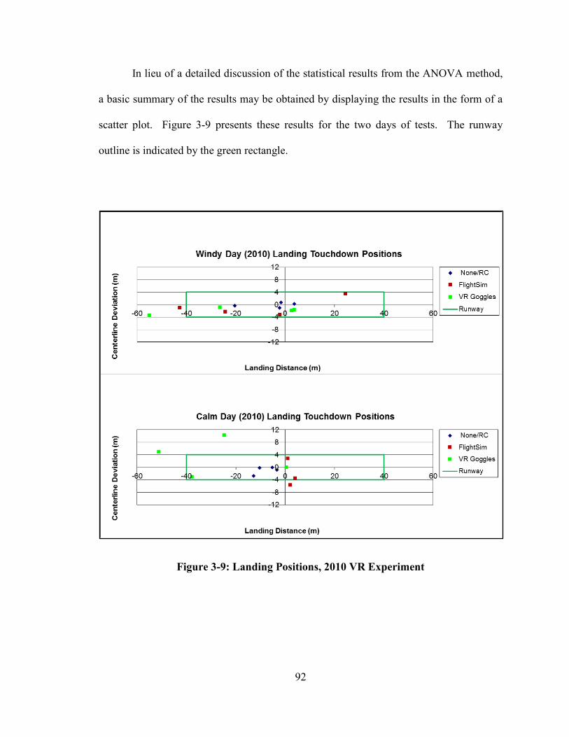
92
In lieu of a detailed discussion of the statistical results from the ANOVA method,
a basic summary of the results may be obtained by displaying the results in the form of a
scatter plot. Figure 3-9 presents these results for the two days of tests. The runway
outline is indicated by the green rectangle.
Figure 3-9: Landing Positions, 2010 VR Experiment
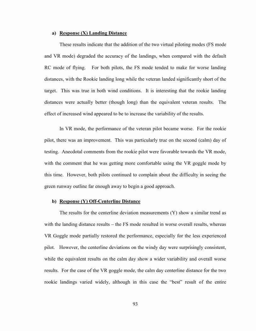
93
a) Response (X) Landing Distance
These results indicate that the addition of the two virtual piloting modes (FS mode
and VR mode) degraded the accuracy of the landings, when compared with the default
RC mode of flying. For both pilots, the FS mode tended to make for worse landing
distances, with the Rookie landing long while the veteran landed significantly short of the
target. This was true in both wind conditions. It is interesting that the rookie landing
distances were actually better (though long) than the equivalent veteran results. The
effect of increased wind appeared to be to increase the variability of the results.
In VR mode, the performance of the veteran pilot became worse. For the rookie
pilot, there was an improvement. This was particularly true on the second (calm) day of
testing. Anecdotal comments from the rookie pilot were favorable towards the VR mode,
with the comment that he was getting more comfortable using the VR goggle mode by
this time. However, both pilots continued to complain about the difficulty in seeing the
green runway outline far enough away to begin a good approach.
b) Response (Y) Off-Centerline Distance
The results for the centerline deviation measurements (Y) show a similar trend as
with the landing distance results – the FS mode resulted in worse overall results, whereas
VR Goggle mode partially restored the performance, especially for the less experienced
pilot. However, the centerline deviations on the windy day were surprisingly consistent,
while the equivalent results on the calm day show a wider variability and overall worse
results. For the case of the VR goggle mode, the calm day centerline distance for the two
rookie landings varied widely, although in this case the “best” result of the entire

94
experiment was accomplished by the Rookie pilot (X=+0.6m, Y=0m). This was one of
the last tests of the day, and it was at this point that the rookie pilot commented that he
was getting more comfortable with this mode of flying.
c) Control Problems with FS Mode
The FS mode suffered from poor ergonomics during this experiment, and most
likely was a main reason for the generally poor results when either pilot used this mode.
The need to twist the body to see the laptop display in the back of vehicle (to provide a
sunshield) was not ideal, especially while using an FM R/C transmitter with its long
(1.5m) antenna. The odd position of this antenna, and its potential shielding so close to a
large metallic object (the vehicle) is the suspected source of radio interference which
resulting in one of the test cases being aborted on Day 2 due to safety concerns.
3.3.3.6 Summary of 2010 VR Landing Results
For the experienced R/C pilot it appeared that the default RC mode was the
method which he was most comfortable using, and seemed the most appropriate
(accurate) method for landing small UAVs under manual control. The addition of VR
technologies did not assist the experienced R/C flier, and appeared to degrade his
performance in terms of landing location accuracy.
For the less experienced flyer, the addition of VR technologies did provide some
assistance, improving the accuracy of precision landings, especially in terms of centerline
deviation (Y). However, the FS mode yielded worse performance. It is very likely that
the poor ergonomics of the makeshift FS mode used during these experiments had a
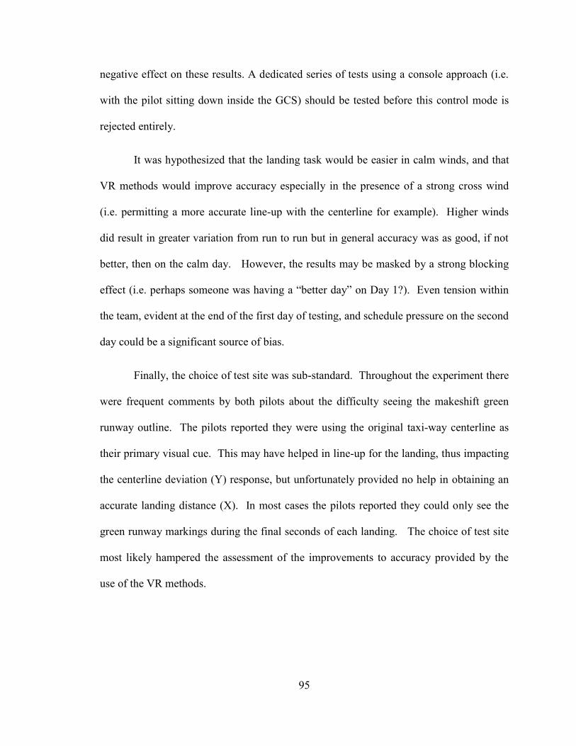
95
negative effect on these results. A dedicated series of tests using a console approach (i.e.
with the pilot sitting down inside the GCS) should be tested before this control mode is
rejected entirely.
It was hypothesized that the landing task would be easier in calm winds, and that
VR methods would improve accuracy especially in the presence of a strong cross wind
(i.e. permitting a more accurate line-up with the centerline for example). Higher winds
did result in greater variation from run to run but in general accuracy was as good, if not
better, then on the calm day. However, the results may be masked by a strong blocking
effect (i.e. perhaps someone was having a “better day” on Day 1?). Even tension within
the team, evident at the end of the first day of testing, and schedule pressure on the second
day could be a significant source of bias.
Finally, the choice of test site was sub-standard. Throughout the experiment there
were frequent comments by both pilots about the difficulty seeing the makeshift green
runway outline. The pilots reported they were using the original taxi-way centerline as
their primary visual cue. This may have helped in line-up for the landing, thus impacting
the centerline deviation (Y) response, but unfortunately provided no help in obtaining an
accurate landing distance (X). In most cases the pilots reported they could only see the
green runway markings during the final seconds of each landing. The choice of test site
most likely hampered the assessment of the improvements to accuracy provided by the
use of the VR methods.

96
3.3.4 Bell Island Landing Experiment (2013)
Due to the inconclusive results in 2010, it was decided that a repeat of the landing
experiment should be done when time and schedule permitted. After a three year hiatus,
the experiment was revived and repeated in November 2013. The test site was reverted
back to the originally planned location at the Bell Island airfield, as shown in Figure 3-10.
The locations of the pilots, side and end cameras and a trailer used as the GCS are noted.
The target point for the landings was between the numbers “26”, directly in front of the
pilots, located 45 m from the end of the runway. The runway is approximately 20 m (66
ft) wide as shown.
Figure 3-10: Test Site at Bell Island Airfield (2013)

97
3.3.4.1 Flight Test Vehicles for 2013
The same class of test vehicle was used for the 2013 repeat, although not the
identical aircraft. The original aircraft used in 2010 was unfortunately lost in a flight
mishap in 2011. Two new GiantStiks were constructed, GBS#10 and GBS#11 to support
the 2013 experiment. As with the 2010 aircraft, electric propulsion was used. During
initial flight tests to shake-down the FPV equipment, GBS#11 was lost at sea north of the
Argentia while investigating interference problems with the video link. The significance
of this unplanned event will be discussed in detailed in Section 3.3.4.6. A third GBS#12
was constructed as a replacement for GBS#11. The idea was that a second aircraft would
always be available in case the primary vehicle (GBS#10) was lost during the experiment.
In the end, this proved un-necessary and GBS#10, as shown in Figure 3-11, performed its
function perfectly and survived.
Figure 3-11: GiantStik#10 Test Vehicle (2013)

98
3.3.4.2 The Pilots of the 2013 Experiment
For the 2013 VR Experiment, a new pair of pilots were recruited:
a) Stephen Crewe (Veteran Pilot), the veteran pilot this time was the primary
manual pilot for Project RAVEN since 2012. Stephen had about 10 years flying
experience flying R/C aircraft at the time of the 2013 VR Experiment. He also
had about one year experience using FPV equipment with his own personal R/C
flying.
b) Dilhan Balage (Rookie Pilot), the rookie pilot this time was a staff engineer from
Project RAVEN whose background is primarily electrical/computer engineering.
He had been flying R/C aircraft only for the previous two flying seasons, and most
of this experience was on the smaller Ultra40 and electric “foamy” type aircraft.
He appeared to be nervous about flying the relatively large GiantStik, but quickly
learned it shared much of the flight characteristics as its smaller cousin (i.e. the
Ultra40). However, Dilhan had limited experience in aviation, apart from his
work with Project RAVEN as an AVO.
3.3.4.3 Updated 2013 VR Equipment
The state of the art of VR equipment has advanced significantly since the original
used in the 2010 experiment. The older equipment was replaced by updated First Person
View (FPV) components, based around the EagleTree series of FPV products. Aimed at
the high-end R/C hobby community, these FPV components are now borderline UAV
avionics sets, including built-in GPS, On-Screen Display (OSD), and a rudimentary
autopilot-capability (Eagle Tree Systems, 2013). For these experiments only the GPS and
OSD features were used.

99
I. Updated Airborne Components
The camera used by the new FPV system is supplied in an integrated pan/tilt turret
format. This was installed on the GiantStik using a custom built mount held to the top of
the main wing using a rubber/plastic band (similar to the aluminum flashing band used in
the 2010 experiment). Suspected RF interference caused by the original idea of using an
aluminum band prompted the switch to the rubber/plastic material. The 2013 airborne
equipment, including the new camera turret mount may be seen Figure 3-15.
Figure 3-12: VR Camera and Turret (2013)
The complete FPV system as installed on the aircraft consisted of the components
shown in the annotated Figure 3-16. The new FPV system used a dedicated 5.8 GHz
high-power video transmitter (C). Initially the normal 5.8 GHz antenna (B) was used, but
this was switched to a special mushroom-shaped bi-polar style antenna (A) which had
superior transmission range, especially when combined with a more powerful transmitter
(i.e. at least 6 km when used with a 600 mW transmitter). For the electric-powered
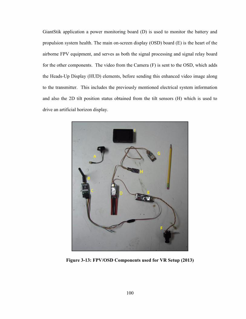
100
GiantStik application a power monitoring board (D) is used to monitor the battery and
propulsion system health. The main on-screen display (OSD) board (E) is the heart of the
airborne FPV equipment, and serves as both the signal processing and signal relay board
for the other components. The video from the Camera (F) is sent to the OSD, which adds
the Heads-Up Display (HUD) elements, before sending this enhanced video image along
to the transmitter. This includes the previously mentioned electrical system information
and also the 2D tilt position status obtained from the tilt sensors (H) which is used to
drive an artificial horizon display.
Figure 3-13: FPV/OSD Components used for VR Setup (2013)

101
The GPS module (G) provides the 3D position of the aircraft, which the OSD uses
to calculate altitude, ground speed and the position of “home base” which is the saved
location when the OSD was first turned on (i.e. the GCS location). The rectangular box
(I) at top is a small solid-state recording device which is part of the Ground Components,
and described in the next section.
II. Ground Components
(a) VR Goggles
The 2013 VR experiment used a new set of FPV goggles from “Fat Shark” (Fat
Shark , 2013). The new style of goggles used can be seen being worn by one of the pilots
in Figure 3-14.
Figure 3-14: Fatshark Goggles used for 2013 Experiment

102
These goggles have a built-in receiver. The new headset also includes pan/tilt
sensors, similar to those in the VR1000, but with much better accuracy and reliability.
The modern FPV equipment also used a solid-state data recorder (i.e. Component I in
Figure 3-13) to record the FPV video, eliminating the need to use a video capture card
(b) Heads-Up Display (HUD)
The FPV equipment featured a HUD display, using the sensors on the aircraft to
measure GPS location and pan/tilt of the aircraft. The OSD module used GPS to calculate
the airspeed, altitude and heading of the aircraft. The direction to “home base” is also
shown. When combined with the pan/tilt sensor, this allowed the display of a HUD.
Figure 3-15 is an example of the display provided to the VR pilots.
Figure 3-15: First Person View (FPV) Display with HUD (2013)

103
The HUD provided the current aircraft position, ground speed (MPH) and altitude
above ground (ft) in the form of “ladders” on the left and right sides respectively, as well
as an artificial horizon. Although this artificial horizon was found to “lag” reality (as
shown in the figure), the altitude and ground speed were accuracy enough to allow for
good “flares” during the VR landings. The items in the lower left and right corners
provided the current power draw and total power consumed by the electrical propulsion
system. Since we used 10,000 mAH of total battery power this display acted like a “fuel
gauge” letting us know when the aircraft power was dropping too low (i.e. when total
power consumed exceeded 8000 mAH). Even in cold weather (1-4ºC), we had flight
endurances of between 20 and 25 minutes on a fully charged set of batteries.
(c) Improved FS Mode Display
For the 2013 experiment a dedicated FPV display screen was used. This was
mounted on a tripod in front of the pilot, as shown in Figure 3-16.
Figure 3-16: FPV Static Display LCD on Tripod/Stand (2013)
104
In addition to improving the ergonomics of having to turn to view an LCD inside
the back of a vehicle, this arrangement eliminated the contradiction due to the pilot’s
aural (hearing) cues being opposite to his visual cues as the aircraft flew past when his
back was turned to the runway. The FPV screen also included a safety feature not
common to most LCDs. The FPV display is an analog device, and will continue to show
the degraded video if the signal strength drops. Even a scratchy black-and-white display
is better than nothing. In practical use, such video drop-outs were of limited duration (1-2
seconds) when flying in FPV mode, assuming the analog method is used and the aircraft
was kept within 1 km range. The VR goggles video also behaves in this manner. The use
of a dedicated FPV display therefore allowed a much better assessment of the
effectiveness of the FS mode during the 2013 experiment.
3.3.4.4 2013 Experimental Results
Following a practice day on 27-November, and dodging cold and rainy weather all
week, the experiment was finally ran on Friday, November 29, 2013. The winds were
down the runway (i.e. almost no cross wind) at 5-7 knots (about 9-13 km/hr). Conditions
were sunny with a few clouds but quite cold (~2ºC). The test cases ran in the morning
were deemed to be “Calm Day” conditions. The results showed a marked improvement
in overall pilot performance versus the 2010 results. The effect of running the
experiment on a proper runway, with aviation-grade markings was clear. Both pilots
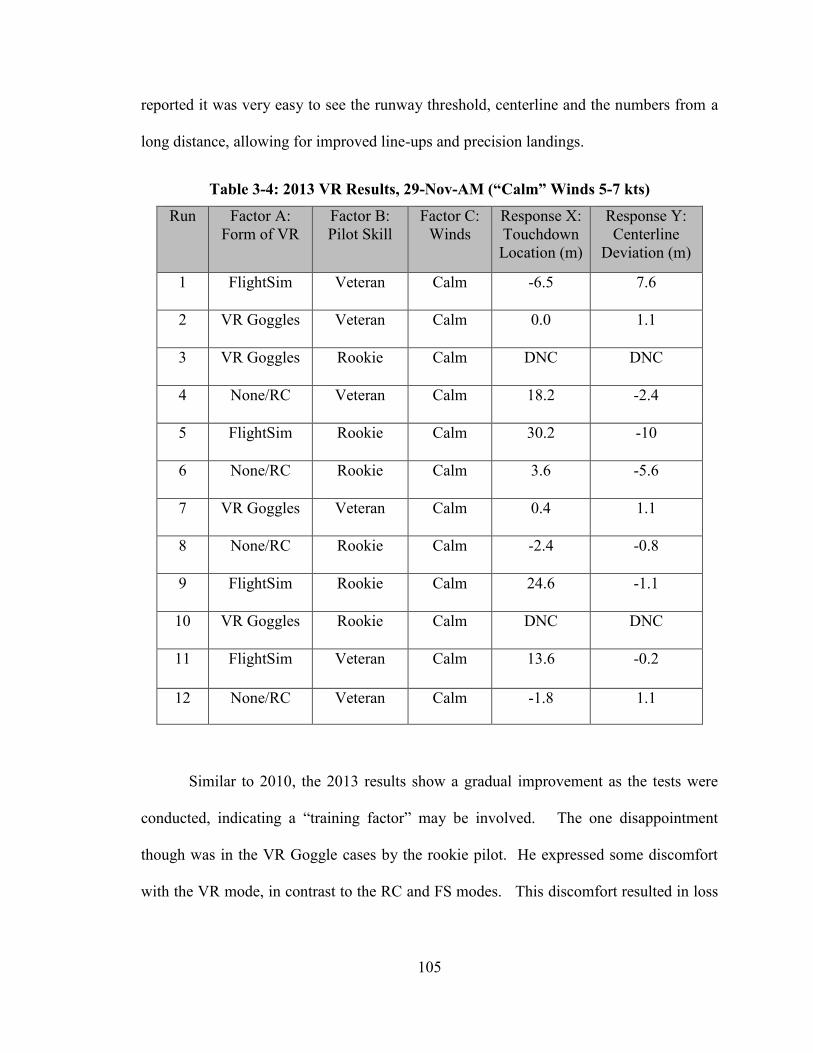
105
reported it was very easy to see the runway threshold, centerline and the numbers from a
long distance, allowing for improved line-ups and precision landings.
Table 3-4: 2013 VR Results, 29-Nov-AM (“Calm” Winds 5-7 kts)
Run Factor A:
Form of VR
Factor B:
Pilot Skill
Factor C:
Winds
Response X:
Touchdown
Location (m)
Response Y:
Centerline
Deviation (m)
1 FlightSim Veteran Calm -6.5 7.6
2 VR Goggles Veteran Calm 0.0 1.1
3 VR Goggles Rookie Calm DNC DNC
4 None/RC Veteran Calm 18.2 -2.4
5 FlightSim Rookie Calm 30.2 -10
6 None/RC Rookie Calm 3.6 -5.6
7 VR Goggles Veteran Calm 0.4 1.1
8 None/RC Rookie Calm -2.4 -0.8
9 FlightSim Rookie Calm 24.6 -1.1
10 VR Goggles Rookie Calm DNC DNC
11 FlightSim Veteran Calm 13.6 -0.2
12 None/RC Veteran Calm -1.8 1.1
Similar to 2010, the 2013 results show a gradual improvement as the tests were
conducted, indicating a “training factor” may be involved. The one disappointment
though was in the VR Goggle cases by the rookie pilot. He expressed some discomfort
with the VR mode, in contrast to the RC and FS modes. This discomfort resulted in loss

106
of orientation, resulting in some erratic flying.. In both VR landing attempts, the situation
deteriorated to the point were safety for the GCS crew was a concern, and the other pilot
had to take emergency control. These are noted in the table as DNC (did not complete).
Following the morning tests, and facing deteriorating team morale and weather, it
was decided to perform a series of “demonstration” runs. The author stepped in to be the
rookie pilot. Only four cases were ran before weather conditions forced a stop to the
experiment. These results are shown in Table 3-4, where “Jon” denotes the cases flown by
this author. Both pilots expressed optimism about the quality of the video feed, and also
the ease of flying well coordinated approaches. The VR Goggle method was not
disorienting for either of us. The accuracy of the approaches, especially in terms of
centerline deviation, is pretty clear. One of the author’s approaches went quite long,
similar to full-sized aircraft “floating” behavior, but landed within 1 m of the runway
centerline. Weather conditions were rapidly deteriorating at this point, as it started to
snow, forcing a stop to the flying activities on this day. This would turn out to be the
final flying of Project RAVEN.
Table 3-5: 2013 VR Results, 29-Nov-PM (“Windy” 9-11 kts)
Run Factor A:
Form of VR
Factor B:
Pilot Skill
Factor C:
Winds
Response X:
Touchdown
Location (m)
Response Y:
Centerline
Deviation (m)
1 None/RC Veteran Windy -6.8 4.8
2 VR Goggles Jon Windy 19.5 2.0
3 FlightSim Jon Windy 88.2 -0.8
4 FlightSim Veteran Windy -2.8 1.8
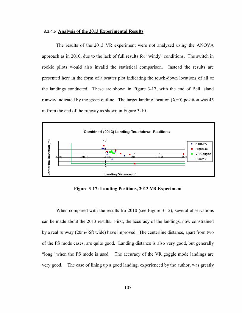
107
3.3.4.5 Analysis of the 2013 Experimental Results
The results of the 2013 VR experiment were not analyzed using the ANOVA
approach as in 2010, due to the lack of full results for “windy” conditions. The switch in
rookie pilots would also invalid the statistical comparison. Instead the results are
presented here in the form of a scatter plot indicating the touch-down locations of all of
the landings conducted. These are shown in Figure 3-17, with the end of Bell Island
runway indicated by the green outline. The target landing location (X=0) position was 45
m from the end of the runway as shown in Figure 3-10.
Figure 3-17: Landing Positions, 2013 VR Experiment
When compared with the results fro 2010 (see Figure 3-12), several observations
can be made about the 2013 results. First, the accuracy of the landings, now constrained
by a real runway (20m/66ft wide) have improved. The centerline distance, apart from two
of the FS mode cases, are quite good. Landing distance is also very good, but generally
“long” when the FS mode is used. The accuracy of the VR goggle mode landings are
very good. The ease of lining up a good landing, experienced by the author, was greatly
108
increased when the immersive VR mode was used. Still, the poor performance of the first
rookie pilot while using the VR mode was a cause for concern. It became evident that
while the VR mode assisted myself and the veteran pilot, both who have flown flight
simulators extensively since adolescence, to a person untrained in “normal” flying the VR
mode does not provide the same advantage. Indeed, Dilhan first learned to fly using RC
mode, and this appears to be the flying style he is most comfortable with. This was a
result those of us involved in aviation had not considered. Generally, learning to fly R/C
aircraft after you already know how to fly “real planes” involves combatting the third
person disorientation effects caused by control reversal. The FPV mode is one way of
skipping this problem altogether.
3.3.4.6 Significance of the Loss of GSB#11
The loss of GBS#11 during initial FPV equipment shakedown, while not a
planned event, is an important result of these VR experiments. It was flown beyond the
range of the FPV video transmitter resulting in a loss of signal, and was too far away to
allow recovery using normal R/C means. This illustrated one of the dangers of using
FPV mode that this author and others have noted – pilots tend to fly much higher and
further than normal R/C flying, possibly in an attempt to emulate full-size aircraft flying
practice, to the point where FPV becomes the only viable means of manual remote
control. The gigantic nature of the runways at Argentia (i.e. 200 foot wide runways) only
served to exacerbate this tendency.
109
Without a reliable BLOS manual control link, the use of R/C methods alone at the
extended ranges encouraged by the use of FPV may render the small UAV uncontrollable.
It is for this reasons that both MAAC and AMA set strict guidelines on the use of FPV
techniques by their members (MAAC, 2012) (AMA, 2014). According to these
guidelines FPV can only be used within unassisted visual range and always with the
presence of a dedicated spotter who is also a second pilot ready to assume normal R/C
control, should the FPV pilot become disorientated or the FPV equipment fail. Also, TC
cautions the UAV operator to not assume that FPV technology alone can provide the
desired situational awareness at BLOS ranges, in terms of providing the “sense and
avoid” function of a manned aircraft pilot (TC TP15263, 2014).
3.3.5 Conclusions from Both VR Experiments
When the results from both VR experiments are considered together there are a
number of important observations and conclusions that may be drawn:
1. The use of a real runway, using aviation grade markings, results in a
significant improvement in VR mode landing accuracy, but has almost no
effect on R/C mode.
2. For someone “entrenched” in the use of R/C alone, the addition of VR
methods may hinder landing accuracy.
3. The VR method appears to be a promising method, but only if used by
pilots familiar with full-size aircraft flying methods, and with sufficient
training.
4. There appears to be a training effect involved in the use of novel VR
methods for UAV control. In the case of both sets of experiments there
was evidence that pilot performance was improving gradually as the test
110
progressed. To someone already trained in the use of FPV methods, such
as the second Veteran pilot, this effect is quite strong.
5. The fixed-view FS mode, while being easier to implement (i.e. not
requiring the tilt sensor or head tracking equipment) appears to be less
accurate then the VR mode. It is possible, especially when the second
(2013) set of results are examined, that there may be a fear factor involved.
Forcing yourself to look at a small FPV screen when you could hear the
aircraft approaching was difficult. The natural tendency for most R/C
pilots is to avoid hitting yourself with your own aircraft! Most R/C pilots
tend to err on the side of safety, and land beyond the pilot position. The
results for the 2013 FS mode in particular appear to show this effect, as the
pilot position was much closer to the runway centerline than in 2010.
6. When flying in FPV mode, pilots have a tendency to fly higher and further
than normal R/C flying. It therefore becomes crucial that sufficient video
feed signal strength (i.e. range) is provided to avoid sudden video signal
drop-outs.
7. The addition of a HUD display improves the quality of the landing
approach and with practice, encourages the use of proper landing speeds
and flared landings.
Following the 2013 experiment, the video footage, especially of the various VR
and FS modes was re-examined from both series of tests. The measurements of landing
distance (X) and centerline deviation (Y) do not tell the complete story. It was noticed
that when flying in R/C mode, the aircraft turns and altitude holding were not as accurate
or smooth as with the FPV modes. When flying FPV, the pilot appears to naturally start
to fly like a full-size aircraft. Turns are gentler with bank angles more typical of manned
aircraft. Altitude, especially with the addition of HUD instruments, is typically held
111
within 50 feet. However, the size of the circuits are much bigger in FPV mode, with the
pilot flying downrange quite some distance before turning onto final approach to land.
Again, this is very similar to full-sized aircraft flying practice.
3.4 Extended Range Video Links at Beyond Line of Sight
Project RAVEN has been testing extended range video, still images and remote
data transfer technologies since 2006. Unfortunately, for a majority of this flight testing,
flight at Beyond Line of Sight (BLOS) range was not permitted due to SFOC restrictions.
However, in the fall of 2013 Project RAVEN was granted an exception and permitted to
fly the first true BLOS mission. To be permitted to do this, a section of airspace north of
the old Argentia airbase would be blocked off and temporarily classified as restricted
airspace (i.e. Restricted Class F airspace). We would also equip the UAV with an
extended range FPV setup, and an extended range telemetry link to maintain the link
between the aircraft autopilot and the GCS throughout the mission.
Figure 3-18 shows the flight plan used for the BLOS mission to Fox Island. The
UAV would launch from the NE end of the main runway, fly 4 km to the island,
circumnavigate it, and then fly back. This flight plan would be repeated for as long as the
aircraft endurance would allow. For this mission one of the gasoline-powered GiantStik
aircraft would be used, equipped with an ArduPilot autopilot system (3DRobotics, 2013).
The GiantStik used featured an enlarged fuel tank which allowed approximately 40-45
minutes of useful flight time.

112
Figure 3-18: Beyond Line of Sight (BLOS) Mission to Fox Island
An extended-range version of the FPV setup as used by the 2013 VR experiment
was used for this mission. Key to this system was the use of a more powerful video
transmitter (i.e. 600 mW power, about three times that normally used by consumer-grade
remote video units). A high-gain antenna suitable for 5.8 GHz was also used, mounted
on top of a 30’ tall radio mast. A second hi-gain antenna suitable for the 900 MHz
Ardupilot telemetry link was also mounted on the mast. In the case of the FPV setup a
diversity RF switching system was used to switch between the hi-gain antenna and the
FPV goggle antenna, depending on the strength of the signal received by both. In theory,
the manual control override system built-in to the Ardupilot system could also have been
used to override the autopilot at BLOS range (provided the telemetry link is maintained),

113
and fly the aircraft based on the FPV video, in a manner very similar to the FS mode in
the VR experiment. However, this was not tested during this initial BLOS mission. The
FPV video was used only to monitor the situation and prove we could maintain a good
video signal at long range (6+ km).
Before we could fly this mission we verified that both the video and telemetry
links could be maintained at a minimum 6 km range. A series of range tests were
conducted in the same area, by setting up both the autopilot GCS and FPV receivers at the
location of an elevated Lookout as shown in Figure 3-18, and flying the aircraft over the
runway, near the GCS location indicated. The range was approximately 2.5 km.
Attenuators were used to deliberately degrade the signal during static tests, to determine
the maximum useful range of both links. The directionality of the hi-gain antennas was
also investigated. In both cases the effect beam width turned out to be quite narrow,
approximately +/- 15º in azimuth and +/-10º in elevation. The sensitivity in elevation was
also marked, especially if the antenna was pointed straight forward or slightly down cast.
This makes sense if multi-path effects are considered.
Following successful range tests of both the FPV and telemetry links, including
drilling of emergency procedures and conducting a mock GCS switchover to a remote
station located at the lookout location (while the UAV was flown over the Argentia
runway), the BLOS was finally conducted on October 30, 2013. A sample image from
the forward FPV camera during this mission may be seen in Figure 3-19.

114
Figure 3-19: FPV View over Fox Island during BLOS Mission
The aircraft was able to travel back and forth and circumnavigated Fox Island
many times during the 45 minutes duration of the mission. The telemetry link between
the ArduPilot and the GCS worked flawlessly. We calculated that the maximum range
was approximately 5.0 km, when the UAV was north of Fox Island. The FPV system
maintained good video quality for most of the mission. The only times of degraded
quality appeared to be brief moments when the aircraft turned the antenna away from the
GCS location, usually during the return track and off to the right of Argentia as seen from
the aircraft. The video footage over Fox Island was good enough for us to spot a small
fishing vessel just north of the island, indicated by the yellow circle in Figure 3-19. This
was well beyond the line of sight of all the crew including the spotters at the GCS, and
confirms the basic utility of FPV to enhance situational awareness at BLOS range.
115
3.5 Synthetic Environments
Synthetic environments are commonly used in the field of Unmanned Aerial
Vehicles to provide a simulation environment where various experimental UAV control
methods and mission planning may be accomplished, without risking actual flight
hardware. In the context of the research outlined in this chapter, a low-cost synthetic
environment was developed, initially to assist in mission planning in the early stages of
the Aerosonde flight program. However, this synthetic environment was expanded and
used in other roles, including use as a potential Beyond Line of Sight (BLOS) situation
display. Details of how this simulation evolved and was used will be explored in the
following sections.
3.5.1 Visualization using a Flight Simulator
A visualization tool was developed that permitted small UAVs to be simulated and
observed in a variety of views, including several external views and also a “virtual pilot”
(i.e. from the cockpit) view. The basis of this simulation was an aerodynamic simulation
of the Aerosonde UAV, developed in MATLAB with the assistance of a third party
aerodynamic library called AeroSIM (Unmanned Dynamics, 2006). This library was
developed specifically for simulating small airframes such as the Aerosonde UAV. This
block set included an interface that could be used to send Flight Dynamic Model (FDM)
state information (i.e. aircraft position, angles and velocities) to either the Microsoft
Flight Simulator 2002 or the FlightGear (FG) flight simulator for use as a visualization
tool. This permitted the creation of a low-cost (i.e. about the cost of two modern desktop

116
PCs) UAV synthetic test environment. This basic simulation environment is shown
schematically in Figure 3-20.
Figure 3-20: Low-cost Single UAV Synthetic Environment
FlightGear (FG) was found to be the better choice of visualization tool in terms of
animation quality, especially frame rate. Also, since it is open-source, it was more easily
customized. This same visualization method was used by the Aerosonde GCS for in-lab
simulation and mission planning using hardware-in-the-loop techniques. Figure 3-21 is a
screen shot showing one of our UAV test vehicles, the GiantStik, flying over the
Clarenville Airfield in this simulated environment. The GiantStik visual model was
created by this author using relatively inexpensive (<$100) 3D modeling tools. The
terrain data was available via free download from the FlightGear website. The
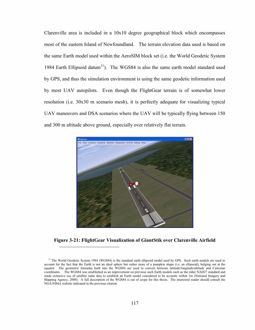
117
Clarenville area is included in a 10x10 degree geographical block which encompasses
most of the eastern Island of Newfoundland. The terrain elevation data used is based on
the same Earth model used within the AeroSIM block set (i.e. the World Geodetic System
1984 Earth Ellipsoid datum11
). The WGS84 is also the same earth model standard used
by GPS, and thus the simulation environment is using the same geodetic information used
by most UAV autopilots. Even though the FlightGear terrain is of somewhat lower
resolution (i.e. 30x30 m scenario mesh), it is perfectly adequate for visualizing typical
UAV maneuvers and DSA scenarios where the UAV will be typically flying between 150
and 300 m altitude above ground, especially over relatively flat terrain.
Figure 3-21: FlightGear Visualization of GiantStik over Clarenville Airfield
11 The World Geodetic System 1984 (WGS84) is the standard earth ellipsoid model used by GPS. Such earth models are used to
account for the fact that the Earth is not an ideal sphere but rather more of a pumpkin shape (i.e. an ellipsoid), bulging out at the equator. The geometric formulae built into the WGS84 are used to convert between latitude/longitude/altitude and Cartesian
coordinates. The WGS84 was established as an improvement on previous such Earth models such as the older NAD27 standard and
made extensive use of satellite radar data to establish an Earth model considered to be accurate within 1m (National Imagery and Mapping Agency, 2000). A full description of the WGS84 is out of scope for this thesis. The interested reader should consult the
NGA/NIMA website indicated in the previous citation.
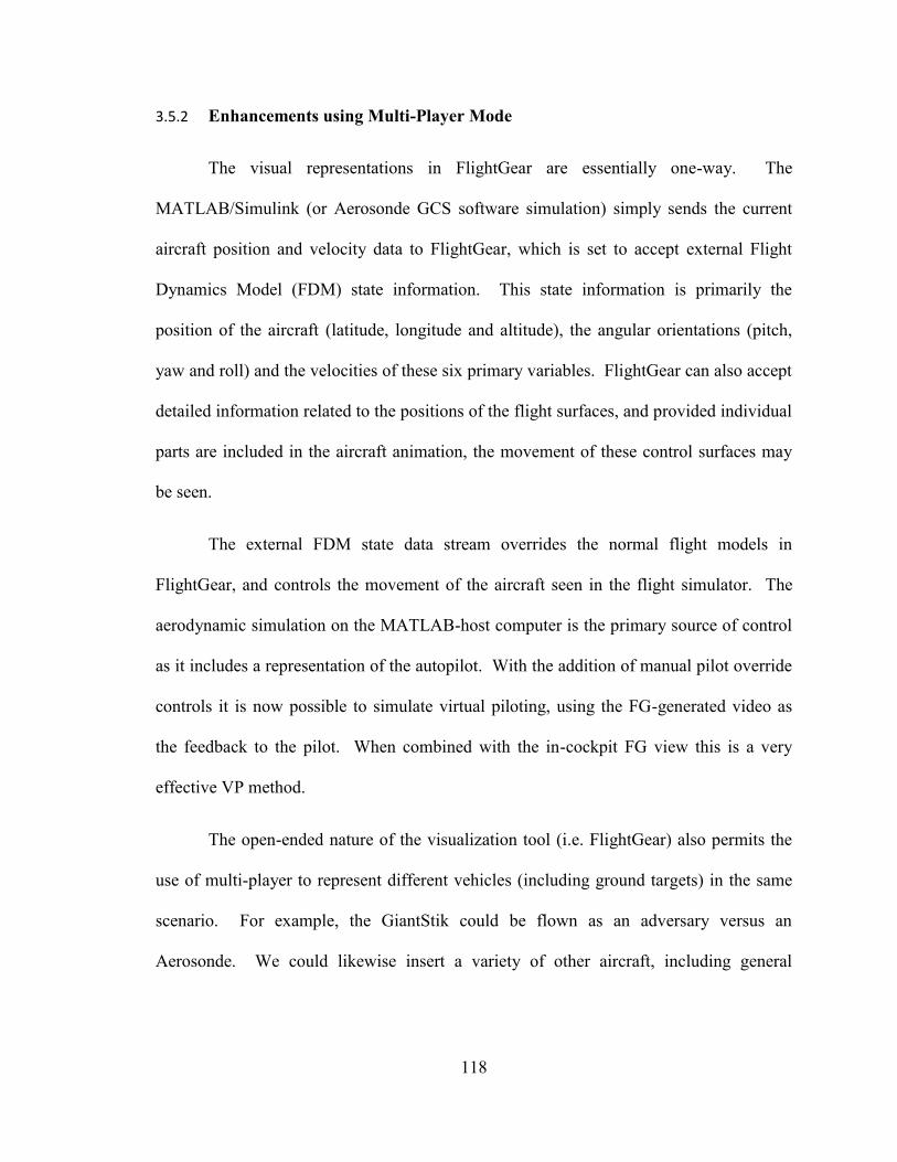
118
3.5.2 Enhancements using Multi-Player Mode
The visual representations in FlightGear are essentially one-way. The
MATLAB/Simulink (or Aerosonde GCS software simulation) simply sends the current
aircraft position and velocity data to FlightGear, which is set to accept external Flight
Dynamics Model (FDM) state information. This state information is primarily the
position of the aircraft (latitude, longitude and altitude), the angular orientations (pitch,
yaw and roll) and the velocities of these six primary variables. FlightGear can also accept
detailed information related to the positions of the flight surfaces, and provided individual
parts are included in the aircraft animation, the movement of these control surfaces may
be seen.
The external FDM state data stream overrides the normal flight models in
FlightGear, and controls the movement of the aircraft seen in the flight simulator. The
aerodynamic simulation on the MATLAB-host computer is the primary source of control
as it includes a representation of the autopilot. With the addition of manual pilot override
controls it is now possible to simulate virtual piloting, using the FG-generated video as
the feedback to the pilot. When combined with the in-cockpit FG view this is a very
effective VP method.
The open-ended nature of the visualization tool (i.e. FlightGear) also permits the
use of multi-player to represent different vehicles (including ground targets) in the same
scenario. For example, the GiantStik could be flown as an adversary versus an
Aerosonde. We could likewise insert a variety of other aircraft, including general
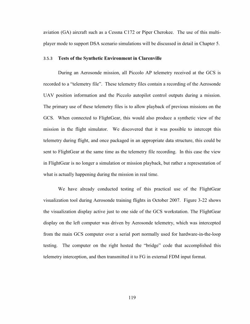
119
aviation (GA) aircraft such as a Cessna C172 or Piper Cherokee. The use of this multi-
player mode to support DSA scenario simulations will be discussed in detail in Chapter 5.
3.5.3 Tests of the Synthetic Environment in Clarenville
During an Aerosonde mission, all Piccolo AP telemetry received at the GCS is
recorded to a “telemetry file”. These telemetry files contain a recording of the Aerosonde
UAV position information and the Piccolo autopilot control outputs during a mission.
The primary use of these telemetry files is to allow playback of previous missions on the
GCS. When connected to FlightGear, this would also produce a synthetic view of the
mission in the flight simulator. We discovered that it was possible to intercept this
telemetry during flight, and once packaged in an appropriate data structure, this could be
sent to FlightGear at the same time as the telemetry file recording. In this case the view
in FlightGear is no longer a simulation or mission playback, but rather a representation of
what is actually happening during the mission in real time.
We have already conducted testing of this practical use of the FlightGear
visualization tool during Aerosonde training flights in October 2007. Figure 3-22 shows
the visualization display active just to one side of the GCS workstation. The FlightGear
display on the left computer was driven by Aerosonde telemetry, which was intercepted
from the main GCS computer over a serial port normally used for hardware-in-the-loop
testing. The computer on the right hosted the “bridge” code that accomplished this
telemetry interception, and then transmitted it to FG in external FDM input format.
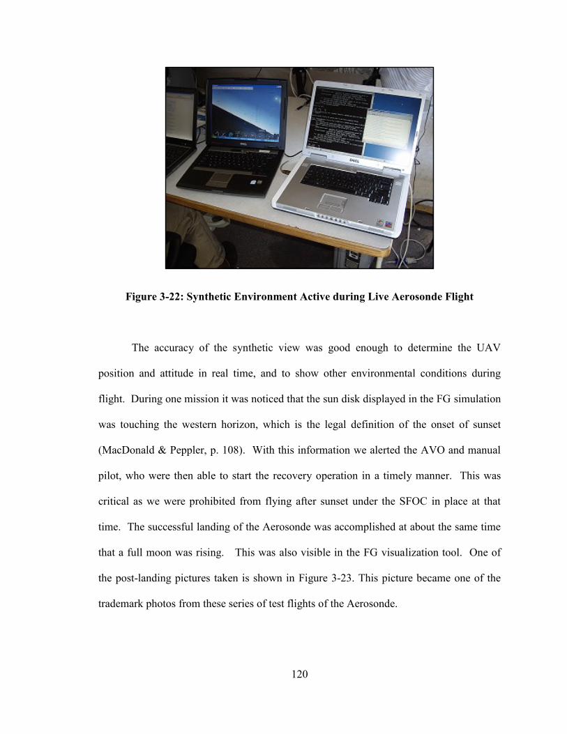
120
Figure 3-22: Synthetic Environment Active during Live Aerosonde Flight
The accuracy of the synthetic view was good enough to determine the UAV
position and attitude in real time, and to show other environmental conditions during
flight. During one mission it was noticed that the sun disk displayed in the FG simulation
was touching the western horizon, which is the legal definition of the onset of sunset
(MacDonald & Peppler, p. 108). With this information we alerted the AVO and manual
pilot, who were then able to start the recovery operation in a timely manner. This was
critical as we were prohibited from flying after sunset under the SFOC in place at that
time. The successful landing of the Aerosonde was accomplished at about the same time
that a full moon was rising. This was also visible in the FG visualization tool. One of
the post-landing pictures taken is shown in Figure 3-23. This picture became one of the
trademark photos from these series of test flights of the Aerosonde.
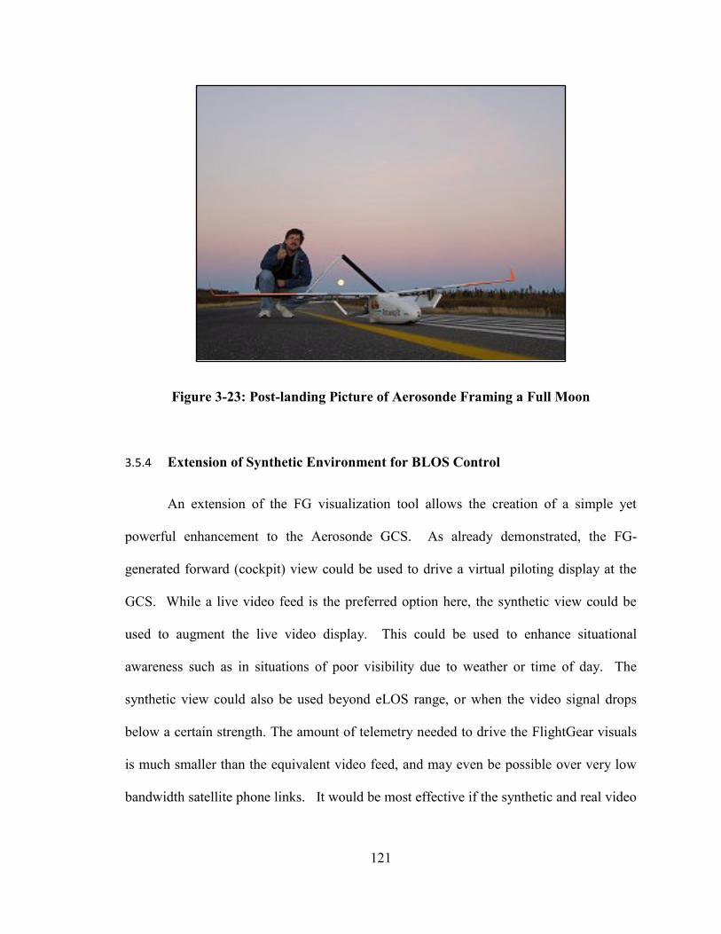
121
Figure 3-23: Post-landing Picture of Aerosonde Framing a Full Moon
3.5.4 Extension of Synthetic Environment for BLOS Control
An extension of the FG visualization tool allows the creation of a simple yet
powerful enhancement to the Aerosonde GCS. As already demonstrated, the FG-
generated forward (cockpit) view could be used to drive a virtual piloting display at the
GCS. While a live video feed is the preferred option here, the synthetic view could be
used to augment the live video display. This could be used to enhance situational
awareness such as in situations of poor visibility due to weather or time of day. The
synthetic view could also be used beyond eLOS range, or when the video signal drops
below a certain strength. The amount of telemetry needed to drive the FlightGear visuals
is much smaller than the equivalent video feed, and may even be possible over very low
bandwidth satellite phone links. It would be most effective if the synthetic and real video
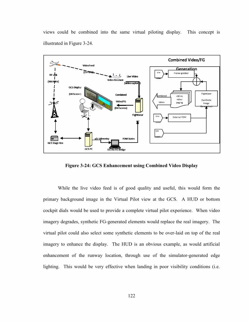
122
views could be combined into the same virtual piloting display. This concept is
illustrated in Figure 3-24.
Figure 3-24: GCS Enhancement using Combined Video Display
While the live video feed is of good quality and useful, this would form the
primary background image in the Virtual Pilot view at the GCS. A HUD or bottom
cockpit dials would be used to provide a complete virtual pilot experience. When video
imagery degrades, synthetic FG-generated elements would replace the real imagery. The
virtual pilot could also select some synthetic elements to be over-laid on top of the real
imagery to enhance the display. The HUD is an obvious example, as would artificial
enhancement of the runway location, through use of the simulator-generated edge
lighting. This would be very effective when landing in poor visibility conditions (i.e.
123
equivalent to IFR with manned aircraft). The synthetic display could also display any
detected entities, either targets on the ground, or other airborne targets nearby, assuming
these are detected via other sensors (e.g. Automatic Identification System (AIS) for ships,
ADS-B, TCAS for cooperative aircraft, etc.), even when these target are well beyond
normal visual range or visible in the video feed.
Most of the pieces needed for this system have been tested within Project
RAVEN, especially the synthetic FG environment and extended range video, however it
must be stressed that a fully-integrated version of the concept illustrated in Figure 3-5
remains a future subject for research, possibly as a focused electrical or computer
engineering project. The concept of combining live-video with synthetic visual
enhancements should be possible even with fairly simple and light-weight electronics. A
form of such an enhanced video, combining real video imagery with synthetic elements,
is the basis of the OSD used by the EagleTree FPV products (Eagle Tree Systems, 2013)
used in the 2013 VR Experiments documented in Section 3.3.4.
3.6 Summary: Effect of Enhanced UAV Control Methods on Safety
An enhanced method to remotely operate a UAV manually could be a significant
improvement to the overall robustness and safety of the system. A FPV view has been
shown, both theoretically and through experiment, to improve the accuracy of precision
flying, if used by a properly trained manual pilot. This improved accuracy should
enhance the safety of UAV flight during takeoffs and landings. The FPV view also
provides a means to accomplish manual emergency landings should the need arise.
124
Instead of the UAV simply crashing into some random location, FPV may be used to
guide the aircraft to a safe dead-stick (i.e. engine out) landing, perhaps on an abandoned
field or road. This emergency landing capability is an important element of manned
aviation safety and trained for by manned aircraft pilots. If applied to small UAV
operations this could represent a significant “mitigation strategy” and would contribute to
a non-zero value in the Pmit term used in equation 2-1.
FPV and enhanced BLOS vision technologies could also be used to improve AVO
situational awareness and reduce the mid-air collision risk12
. The enhanced range FPV
view, if combined with synthetic enhancements, would benefit UAV operations in times
of reduced visibility. Traffic de-conflicting also becomes a possibility should manned
aircraft be encountered and an emergency avoidance maneuver become necessary.
Without such a system, the AVO is indeed blind, and would have no chance to do
anything about the situation. This is one of the primary complaints of small UAVs in
their present form. Any improvement in situational awareness should provide an
improvement to the PUAVfailure (i.e. the chance that the UAV fails to avoid a collision) term
in equation 2-2.
12 It should be noted that Transport Canada does not give much credit to the use of FPV technology as a possible sense and avoid
technology in its present form (TC SI-623-001, 2014). However, with sufficient development, especially if a BLOS synthetic environment could be fused with data from a DSA system, it could one day become an integral part of a possible BLOS remote
piloting system.

125
Chapter 4 Enhancements to UAV Visibility
In this chapter we will explore methods and technologies which may be used to
enhance the visibility of the small UAV. This of course is directly related to the Mid-Air
Collision threat posed by the small UAV. We will begin by determining the theoretical
limits of the “See and Avoid” principal when dealing with the small UAV. This will be
followed by the results from the research of several proposed visibility enhancements,
including:
1. A thorough study of a possible lighting system for the UAV;
2. Using transponder technologies to enhance UAV detectability; and,
3. Providing the UAV with an air-band radio capability.
The goal is to improve the chances that others in the same airspace will be able to
spot the small UAV with sufficient warning to avoid traffic conflicts, thus addressing
Quadrant 2 of the DSA Situation as shown in Table 1-1 (i.e. “Can the UAV be seen and
avoided?). Note also that the concept of “visibility” must be extended to include non-
visual detection means, especially if operation of the small UAV in non-visual weather
conditions is to be contemplated.
4.1 Theoretical Visibility Estimates
In this section, the probability that a small UAV would be seen by a manned
aircraft will be estimated. In addition to the small UAV, the detection ranges for different
sized manned aircraft will be included. These may be used to create a preliminary
126
specification for the requirements of a hypothetical UAV vision/sensing system. The
ability of a pilot to see another aircraft is of course directly related to human visual acuity,
which will be summarized first.
4.1.1 The Human Factors of Vision
Perhaps the most important ability of a human pilot is the sense of sight. It has
been suggested that up to 80% of the sensor input used by humans comes from the eyes
(Chapanis, 1996), and this is especially true for the human pilot. The human eye is
extraordinarily sensitive and has remarkable detection capabilities, although these
capabilities have limitations.
4.1.1.1 Visual Acuity
The visual acuity (i.e. resolving ability) of the human eye varies depending on the
type of detection being attempted and background illumination level. In general, visual
acuity decreases as the complexity of the target detection task increases or when
background illumination is low (Chapanis, 1996, p. 218). In increasing order of difficulty
(and decreasing acuity) these tasks may be classified as:
1. Detection (detecting the presence of something);
2. Vernier (detecting misalignments);
3. Separation (resolving gaps between parts, lines, dots, etc.); and,
4. Identification (letters, object classifications, etc.)
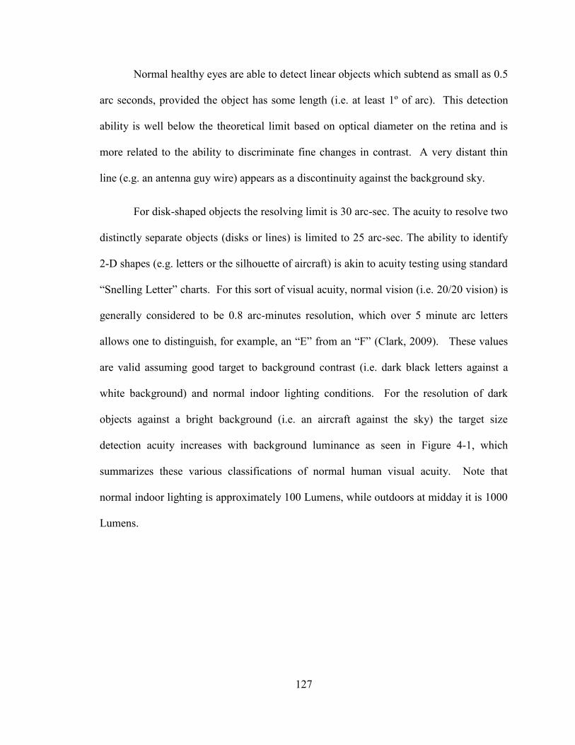
127
Normal healthy eyes are able to detect linear objects which subtend as small as 0.5
arc seconds, provided the object has some length (i.e. at least 1º of arc). This detection
ability is well below the theoretical limit based on optical diameter on the retina and is
more related to the ability to discriminate fine changes in contrast. A very distant thin
line (e.g. an antenna guy wire) appears as a discontinuity against the background sky.
For disk-shaped objects the resolving limit is 30 arc-sec. The acuity to resolve two
distinctly separate objects (disks or lines) is limited to 25 arc-sec. The ability to identify
2-D shapes (e.g. letters or the silhouette of aircraft) is akin to acuity testing using standard
“Snelling Letter” charts. For this sort of visual acuity, normal vision (i.e. 20/20 vision) is
generally considered to be 0.8 arc-minutes resolution, which over 5 minute arc letters
allows one to distinguish, for example, an “E” from an “F” (Clark, 2009). These values
are valid assuming good target to background contrast (i.e. dark black letters against a
white background) and normal indoor lighting conditions. For the resolution of dark
objects against a bright background (i.e. an aircraft against the sky) the target size
detection acuity increases with background luminance as seen in Figure 4-1, which
summarizes these various classifications of normal human visual acuity. Note that
normal indoor lighting is approximately 100 Lumens, while outdoors at midday it is 1000
Lumens.
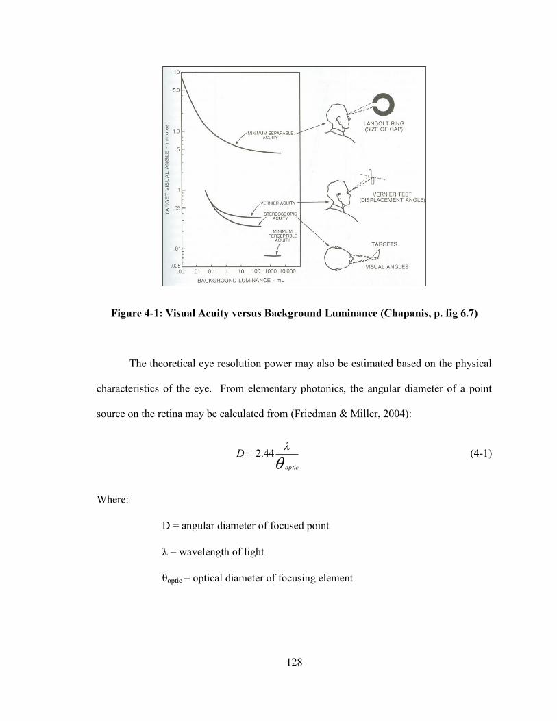
128
Figure 4-1: Visual Acuity versus Background Luminance (Chapanis, p. fig 6.7)
The theoretical eye resolution power may also be estimated based on the physical
characteristics of the eye. From elementary photonics, the angular diameter of a point
source on the retina may be calculated from (Friedman & Miller, 2004):
optic
D 44.2 (4-1)
Where:
D = angular diameter of focused point
λ = wavelength of light
θoptic = optical diameter of focusing element
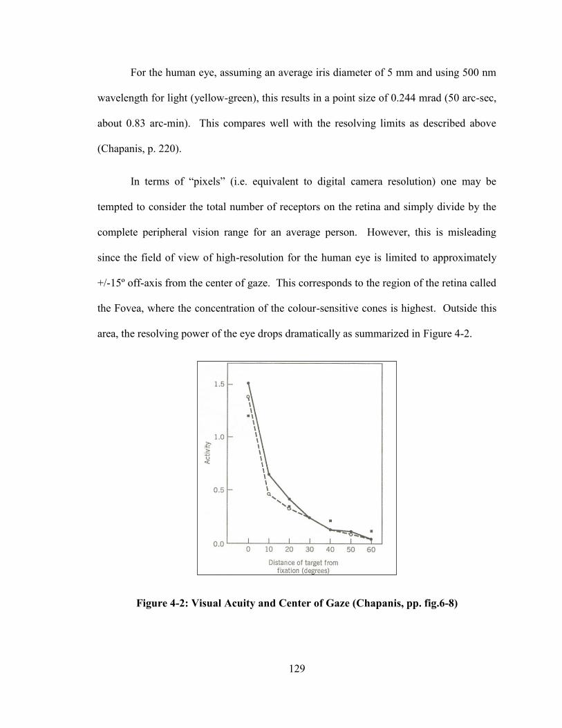
129
For the human eye, assuming an average iris diameter of 5 mm and using 500 nm
wavelength for light (yellow-green), this results in a point size of 0.244 mrad (50 arc-sec,
about 0.83 arc-min). This compares well with the resolving limits as described above
(Chapanis, p. 220).
In terms of “pixels” (i.e. equivalent to digital camera resolution) one may be
tempted to consider the total number of receptors on the retina and simply divide by the
complete peripheral vision range for an average person. However, this is misleading
since the field of view of high-resolution for the human eye is limited to approximately
+/-15º off-axis from the center of gaze. This corresponds to the region of the retina called
the Fovea, where the concentration of the colour-sensitive cones is highest. Outside this
area, the resolving power of the eye drops dramatically as summarized in Figure 4-2.
Figure 4-2: Visual Acuity and Center of Gaze (Chapanis, pp. fig.6-8)
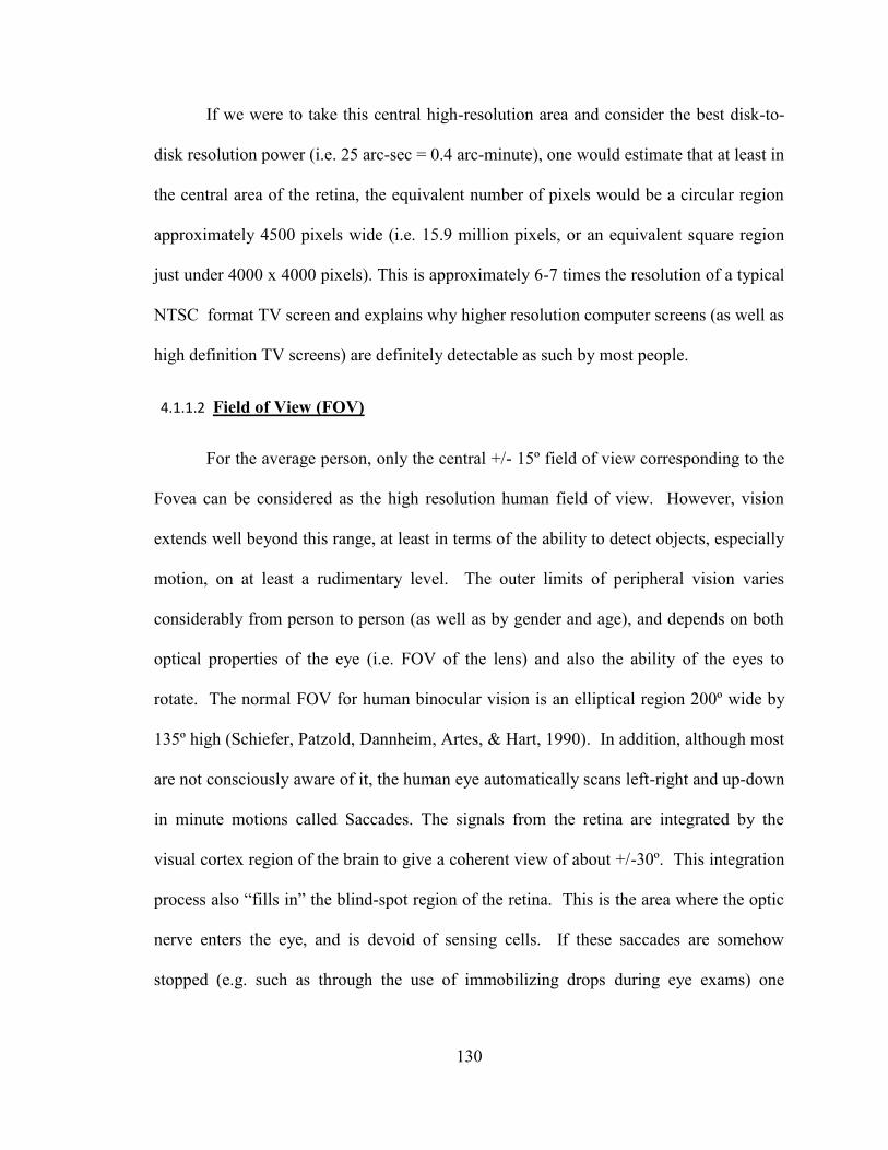
130
If we were to take this central high-resolution area and consider the best disk-to-
disk resolution power (i.e. 25 arc-sec = 0.4 arc-minute), one would estimate that at least in
the central area of the retina, the equivalent number of pixels would be a circular region
approximately 4500 pixels wide (i.e. 15.9 million pixels, or an equivalent square region
just under 4000 x 4000 pixels). This is approximately 6-7 times the resolution of a typical
NTSC format TV screen and explains why higher resolution computer screens (as well as
high definition TV screens) are definitely detectable as such by most people.
4.1.1.2 Field of View (FOV)
For the average person, only the central +/- 15º field of view corresponding to the
Fovea can be considered as the high resolution human field of view. However, vision
extends well beyond this range, at least in terms of the ability to detect objects, especially
motion, on at least a rudimentary level. The outer limits of peripheral vision varies
considerably from person to person (as well as by gender and age), and depends on both
optical properties of the eye (i.e. FOV of the lens) and also the ability of the eyes to
rotate. The normal FOV for human binocular vision is an elliptical region 200º wide by
135º high (Schiefer, Patzold, Dannheim, Artes, & Hart, 1990). In addition, although most
are not consciously aware of it, the human eye automatically scans left-right and up-down
in minute motions called Saccades. The signals from the retina are integrated by the
visual cortex region of the brain to give a coherent view of about +/-30º. This integration
process also “fills in” the blind-spot region of the retina. This is the area where the optic
nerve enters the eye, and is devoid of sensing cells. If these saccades are somehow
stopped (e.g. such as through the use of immobilizing drops during eye exams) one

131
experiences a pronounced narrowing of the field of view (i.e. “tunnel vision”) and in
some cases a pronounced “blind spot” just off-axis from the center of gaze (Friedman &
Miller, p. 138).
Figure 4-3: Practical FOV Limits (Chapanis, pp. fig.4-5)
Of course, the pilot can also turn his head. The ergonomics of this situation have
been studied at length to determine practical limits for this head motion, especially in the
design of man-machine interfaces, for example aircraft cockpits or the interiors of
automobiles. Figure 4-3 gives a summary for normal human operators when taking into
132
account the most acute eye FOV, eye rotation and head turning. As shown the neutral
human line-of-sight is angled downwards at 15º from horizontal, which explains the most
common arrangement seen in aircraft cockpits and automobile dashboards. From an
ergonomic standpoint, it is important to not rely on frequent and continuous head turning.
While it is possible to turn your head back and forth perhaps every other second, to do so
continuously would rapidly become very tiresome. For this reason, the most important
information (e.g. front windows and flight instruments) should be kept within a relatively
narrow forward region (perhaps 30º wide), but additional information (side windows,
radio and engine controls, etc.) can be placed over a wider horizontal and vertical area
(Chapanis, 1996).
It is interesting to note that during particularly intense maneuvers (e.g. final
approach during aircraft landings), human factor researchers including this author have
noticed that most pilots have already fixed their gaze more or less in the forward
direction, with very little side-to-side head motions, as they become fixated on the target
in front of them (Hobbs, p. 11). Any scanning at this point is limited to the view directly
out the front of the aircraft, and the most important cockpit instruments, such as airspeed,
rate of descent, altitude, and the ILS glide-slope indicator. This tendency (“target
fixation”) is frequently cited in aviation accident reports as a major limitation of the “See
and Avoid” principle (TSB Report A00O0057, 2000).

133
4.1.1.3 Sensitivity (Night Vision)
The sensitivity of the human eye to bright light sources, especially at night, is
important in the detection of lights on aircraft, especially the anti-collision strobe. Once
adapted to dark conditions, the sensitivity of the human eye increases by several orders of
magnitude (approximately x106), but generally at the expense of the ability to distinguish
colours (Wandell, 1995). In the early years of nuclear physics, dark-adapted humans eyes
(usually those of graduate students!) were noted as being the most sensitive instruments
for detecting very small numbers of particle (photon) emissions. Legend was that they
could detect a single photon, although later experiments showed that a burst of 5 or more
photons over a particular timeframe is required to be detectable by the human visual
system (Friedman & Miller, p. 138).
Figure 4-4: Densities of Receptors of the Human Eye (Osterberg, 1935)

134
The large increase in eye sensitivity in low light conditions is explained by the
dilation of the iris and also the increased light sensitivity of the rods in the retina. While
most of the colour-sensitive cones are concentrated in the fovea region, the rest of the
retina is covered by the more plentiful (and sensitive) rods. Figure 4-4 shows a summary
of the measured densities of rods and cones in a typical human eye (x1000 per mm2),
where the complementary nature of the two may be seen. Note the gap due to the blind
spot (Osterberg, 1935).
In theory, in dark (starless and moonless) night conditions, a human pilot might be
able to detect the anti-collision lights of another aircraft from as few as 1 to 5 photons (for
black/white) and 10 to 15 photons for colour determination. The smallest detectable
luminance is approximately 10-6
milli-lumens (Chapanis, pp. Table 6-2). Of course, the
inside of an aircraft cockpit at night will not be completely dark. The actual sensitivity of
the pilot’s eyes at night will likely be an average of night-adapted vision and the light
conditions inside the cockpit. Red back-lighting is typically used, as this has been shown
to cause the least amount of degradation of night-adapted human eyesight (AOA, 2014).
We will return to this discussion of night visibility in the section on aircraft lighting
systems in this chapter.
4.1.2 Day-Time Visibility
The human factors summarized in the previous section may now be applied to
estimate the limits of the human pilot in terms of the ability to detect another aircraft
during day time VMC conditions.

135
4.1.2.1 Maximum Detection Range based on Photonics
From elementary photonics, the angular size (radians) of an object of size L, at a
distance D from the observer may be calculated from:
D
LArc
2tan2 (radians) (4-2)
Which for small angles (i.e. θ < 10º), may be simplified as:
D
L)60)(3.57( (arc-min) (4-3)
Either equation may be used in conjunction with human visual acuity limits to estimate
the maximum (ideal) detection range. Alternatively, we may also estimate the smallest
detectable target at a given range. Consider the head-on view of three aircraft shown
approximately to scale in Figure 4-5.
Figure 4-5: Head-on Views of Three Different Aircraft

136
In Figure 4-5, the small size of the Aerosonde (3m/10ft wingspan) is apparent
when compared to a typical GA aircraft (Cessna C172, 11m/36ft wingspan) and the larger
twin-turboprop King Air (16.6m/54.5ft wingspan). If we consider the characteristic
geometries of all three aircraft, we may idealize them as:
(a) A slender horizontal bar (wings); and,
(b) A prominent central disk (fuselage).
Next, consider the minimum legal sighting distance under current VFR rules,
which is 1 statute mile (1609 m) in uncontrolled G class airspace above 1000 feet
(MacDonald & Peppler, p. 115). From this distance, the ability to detect the wings will be
limited by the very slender nature of airfoils. However, the eye can detect very fine linear
objects subtending as low as 0.5 arc-sec. At 1609 m this equates to a thickness of only 4
mm (e.g. an antenna guy wire). However, this ability exists only if the object also
subtends at least 1º of arc in length (Chapanis, 1996). Using this later limit we may
estimate that the minimum detectable wingspan at this range as:
1609)60)(3.57(deg)min/60deg)(1( minL
arc
mL 28min
This suggests that none of these aircraft have wide enough wingspans to be
detected, at least based on the eye’s ability to detect long thin objects. However, the
fuselage might be easier to spot. Assuming a best-case detection limit is 30 arc-sec,

137
which is the absolute limit for human vision in bright lighting, we might estimate the
minimum diameter detectable as:
30 arc-sec/60 =
1609)60)(3.57(min5.0
minarc
m234.0min
This is approximately the diameter of the Aerosonde fuselage. The Cessna
fuselage is approximately 1.52m (5ft) diameter while the King Air is 2.1m (7ft) diameter.
Therefore, it seems the Aerosonde is at the lower limit of detection at 1609m, while the
two larger aircraft would theoretically be detectable at longer range, the Cessna at 10.2
km, and the King Air at 14.6 km. However, we must be careful when using these
estimates as they are based on ideal object to background contrast, laboratory lighting
conditions, and prolonged attention by the observer. This is also detection of a point
object, which is hardly enough to recognize another aircraft. Under practical conditions,
especially time-limited detection tasks, the assumed human visual acuity limit (i.e. 30 arc-
sec in this case) could be lower by a factor of ten (Chapanis, 1996). There is also the
effect of whether an un-cued pilot would even be scanning the right area of the sky for
maximum visual acuity to apply.
Based on the AFRL results (i.e. F-16, of similar size as the Cessna, detected at a
maximum range of 3 km by the average USAF pilot), a scale factor of approximately 3.3
seems appropriate (McCalmont, et al., 2007). Hence, the adjusted maximum detection
ranges would be 488 m for the Aerosonde, 3.1 km for the Cessna and 4.4 km for the King
138
Air. The Cessna and King Air detection ranges comply with the VFR visibility rules, but
the Aerosonde is too small to be detectable at a minimum 1.6 km (1 mi) range.
4.1.2.2 Maximum Detection Range Estimate based on Johnson’s Criteria
An alternative estimate of detection range may be made based on Johnson’s
criteria. These criteria were developed for the U.S. Army in the 1950s to estimate the
target size required by an observer (sensor or human) to accomplish an observation task
with 50% success rate (Friedman & Miller, pp. 4-5). These criteria are:
1. Detection (i.e. The presence of something) – 0.5 to 1.0 line pairs;
2. Orientation (including estimate of motion direction) – 2 to 3 line pairs;
3. Reading Alphanumeric (English characters) – 2.5 to 3 line pairs;
4. Recognition (i.e. is it a tank or artillery piece?) – 3 to 4 line pairs; and,
5. Classification (i.e. is it a T-72 or Sheridan tank?) – 6+ line pairs.
A line pair is one way to define spatial resolution. It is equal to a dark bar and a
white space (often also called one cycle) across the critical dimension of the target.
Crudely, the number of pixels is approximately twice the number of cycles (Friedman &
Miller, p. 6). The critical dimension is usually the diameter or width (across a uniform
disk or square shape, respectively). For an irregular shape it may be estimated as the
square of the area. These criteria have continued to be used during the development of
targeting systems into the 1980s. Recent researchers have also extended them to the
analysis of digital imagery (Vollmerhausen, 1999). Estimates of the probability of
success have been modeled successfully using these relationships:

139
E
E
N
N
N
N
NP
50
50
1
)( (4-4)
Where:
N50 = Number of cycles needed to be resolved across the target dimension for 50 percent
of the observers to get the target choice correct (with the probability of chance
subtracted); target dimension is typically taken as the square root of target area.
N = Number of cycles actually resolved across the target.
E = An empirical scaling factor, equal to:
50
5.07.1N
NE (4-5)
The empirical scaling factor (E) is the outcome of over four decades of target observation
model development (including field tests) and was the currently accepted form as of 2004
(Friedman & Miller, pp. 11-12).
The application of Johnson’s Criteria, and in particular equations 4-4 and 4-5, to
determine the probability of success in four levels of target detection may be summarized
as shown in Figure 4-6. The number of pixels required to successfully accomplish a
certain observation task increases with the task complexity.
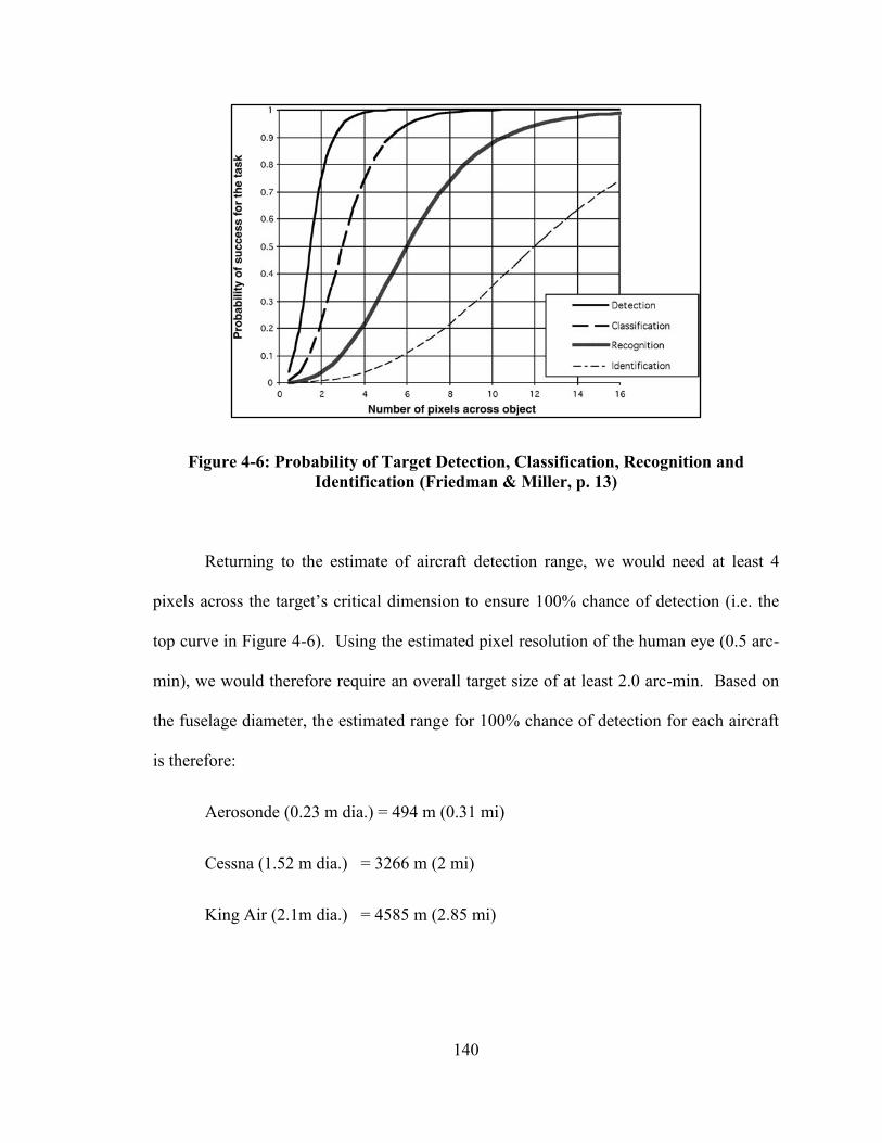
140
Figure 4-6: Probability of Target Detection, Classification, Recognition and
Identification (Friedman & Miller, p. 13)
Returning to the estimate of aircraft detection range, we would need at least 4
pixels across the target’s critical dimension to ensure 100% chance of detection (i.e. the
top curve in Figure 4-6). Using the estimated pixel resolution of the human eye (0.5 arc-
min), we would therefore require an overall target size of at least 2.0 arc-min. Based on
the fuselage diameter, the estimated range for 100% chance of detection for each aircraft
is therefore:
Aerosonde (0.23 m dia.) = 494 m (0.31 mi)
Cessna (1.52 m dia.) = 3266 m (2 mi)
King Air (2.1m dia.) = 4585 m (2.85 mi)

141
These calculations based on Johnson’s Criteria agree well with the previous
photonic estimates assuming the inclusion of the AFRL scale factor (i.e. Aerosonde = 488
m, Cessna = 3.1 km, King Air = 4.4 km) as in Section 4.1.2.1. We can conclude that the
minimum detection range for the Aerosonde UAV is approximately 500 m.
4.1.2.3 Effect of Human Field of View (i.e. Visual Scanning)
When combined with eyeball and modest head rotation, the region of good
scanning is generally defined as a 60º wide cone out front. First, we consider the drop in
visual acuity as an object appears further away from the center of gaze. To model this
effect, we apply a curve fit to human eye visual acuity curve in Figure 4-2 and find that an
exponential curve fits the measured acuity as shown in Figure 4-7.
Figure 4-7: Curve Fit to Off-Axis Visual Acuity
Acuity versus Off-Axis Angle
y = 1.5e-0.0579x
0
0.2
0.4
0.6
0.8
1
1.2
1.4
1.6
0 20 40 60 80 100
Off-axis Angle
Ac
uit
y

142
If we take 1.5 as maximum (ideal) visual acuity, we may estimate the maximum
detection range (Rmax) of a fuselage ( fuselage ) over a range of angles from the center of
gaze by using Equation 4-3:
75.0))(60)(3.57(
)60)(3.57(min75.0
,)60)(3.57(min)5.0)(5.1(
max
max
max
fuselage
fuselage
fuselage
acuityR
Racuity
arc
Racuity
arc
(4-6)
Applying equation 4-6 for the three aircraft being considered over a range of
viewing angles off the center of gaze, we obtain the results as seen in Figure 4-8.
Figure 4-8: Detection Range as a Function of Off-Axis View Angle
Adjusted Detection Ranges
0
500
1000
1500
2000
2500
3000
3500
4000
4500
5000
0 20 40 60 80 100
Off-Axis View Angle
Ma
x.R
an
ge
(m)
Aerosonde
Cessna
KingAir

143
We can now use the estimated drops in visual acuity to calculate the modified
chance of target detection for our aircraft at 1609m (1 mi) range, using the Johnson’s
Criteria method of the previous section. These results are summarized in Figure 4-9, and
show a marked drop in detection range (and probability of detection) off-axis from a fixed
forward gaze. This shows the danger inherent with the “target fixation” problem. Another
aircraft could literally blind-side the pre-occupied pilot. However, assuming the pilot
continues to maintain a good visual scan, the forward 60º view should be monitored fairly
evenly every few seconds.
Figure 4-9: Probability of Detection at 1609m (1 mi)
The effect of pilot visual scanning is difficult to quantify precisely but may be
approximated as follows. The azimuth angle as seen in Figure 4-8 and Figure 4-9 will be
blurred by approximately 20º. Therefore, the visual acuity in the 0-5º range will extend
Probability of Detection at 1 Mile
0.0%
20.0%
40.0%
60.0%
80.0%
100.0%
120.0%
0 20 40 60 80 100
Off-axis View Angle (deg)
Ch
an
ce o
f D
ete
cti
on
(%
)
Aerosonde
Cessna
KingAir
144
out to 20-25º range, and all subsequent results will be as shown, only shifted 20º. Even
with this broadened scan area, the detectability for an aircraft approaching from an
azimuth angle of only 40º or more would still be quite low (< 20%) even for the largest
aircraft being considered here. In the case of the very small Aerosonde, without any form
of visibility enhancements, detectability at 1609m (1 mi) will be near impossible even
when approaching head-on.
4.1.2.4 Safety Aspects of Daytime Visual Detection
Preliminary estimates of the maximum detection ranges for three aircraft have
been made using several different techniques. Based on these results, the safety of the
minimum sighting rules seen in current Aviation Regulations may be called into question.
Assuming a head-approach direction, the Cessna and King Air could be detected at a
maximum range of 3.2 km (2 mi) and 4.6 km (2.85 mi) respectively, assuming ideal
lighting conditions and that the pilot is actively scanning. Detection beyond 4.8 km (3
mi) seems unlikely. The Aerosonde is very small and would only be detected at close
range of 500m (1640 ft) even under ideal conditions.
The danger of an aircraft approaching at some off-axis angle (>40º) is also clear, if
human visual scanning is relied upon. Unless a pilot is actively searching for other
aircraft, it is unlikely he would be looking in the right area of sky to detect the aircraft in
time before it approaches to very close range. This is in fact the typical scenario in most
air-to-air near misses reported, especially for GA aircraft (Hobbs, 1991). Accident
investigation reports involving mid-air collisions universally acknowledge the limitations
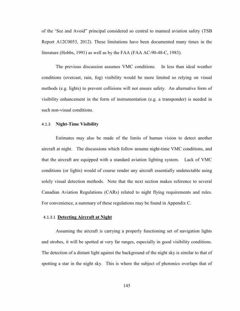
145
of the ‘See and Avoid” principal considered so central to manned aviation safety (TSB
Report A12C0053, 2012). These limitations have been documented many times in the
literature (Hobbs, 1991) as well as by the FAA (FAA AC-90-48-C, 1983).
The previous discussion assumes VMC conditions. In less than ideal weather
conditions (overcast, rain, fog) visibility would be more limited so relying on visual
methods (e.g. lights) to prevent collisions will not ensure safety. An alternative form of
visibility enhancement in the form of instrumentation (e.g. a transponder) is needed in
such non-visual conditions.
4.1.3 Night-Time Visibility
Estimates may also be made of the limits of human vision to detect another
aircraft at night. The discussions which follow assume night-time VMC conditions, and
that the aircraft are equipped with a standard aviation lighting system. Lack of VMC
conditions (or lights) would of course render any aircraft essentially undetectable using
solely visual detection methods. Note that the next section makes reference to several
Canadian Aviation Regulations (CARs) related to night flying requirements and rules.
For convenience, a summary of these regulations may be found in Appendix C.
4.1.3.1 Detecting Aircraft at Night
Assuming the aircraft is carrying a properly functioning set of navigation lights
and strobes, it will be spotted at very far ranges, especially in good visibility conditions.
The detection of a distant light against the background of the night sky is similar to that of
spotting a star in the night sky. This is where the subject of photonics overlaps that of

146
astronomy. The anecdotal comment within the astronomy community is that properly
dark-adapted human eyes are capable of detecting sky objects down to a magnitude of +6,
though some claim as high as +8 (Clark, 2009). Here we are using the relative magnitude
scale used by Astronomers since antiquity, and which was originally based on the order
(or “class”) in which stars appear to the naked eye as the night sky darkens after sunset.
6th
magnitude stars were by definition considered the faintest observable by unaided
eyesight (Keill, 1739). This magnitude scale has been expanded upwards and downwards
more or less using a logarithmic scale, especially to cover the situation of very faint
objects that are normally invisible to the naked human eye. This magnitude scale is
interesting from an historical perspective, but for practical calculations we need to relate
human eyesight capabilities to engineering units and quantities.
Fortunately, much work has been done to characterize the capabilities of the eye,
especially at night, for obvious reasons of flight safety. The light intensity requirements in
the aviation regulations imply a detection range of at least 3.2km (2 mi) (MacDonald &
Peppler, p. 109). The ability to detect an illumination source is directly related to its
contrast against the background luminance of the scene. For example, attempting to spot
the light of an aircraft against a dark night is much easier than against a busy background
(e.g. town/city with lights), or a night sky dominated by sky glow or a full moon. The
minimum detection threshold for a human eye-sight has been studied extensively,
including studies of the special situation for human pilots viewing scenes close to the
ground (Federal Aviation Administration, 1997). A useful correlation has been developed
for this situation versus the background luminance (B) as follows:
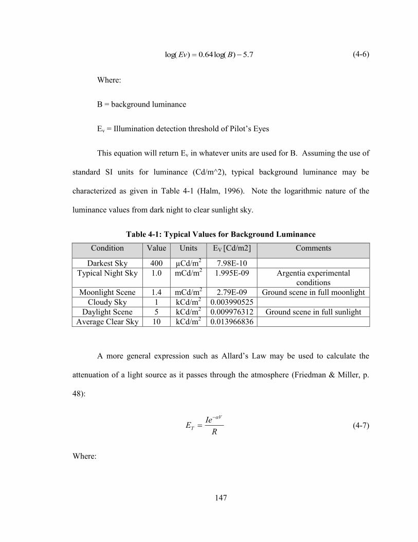
147
7.5)log(64.0)log( BEv (4-6)
Where:
B = background luminance
Ev = Illumination detection threshold of Pilot’s Eyes
This equation will return Ev in whatever units are used for B. Assuming the use of
standard SI units for luminance (Cd/m^2), typical background luminance may be
characterized as given in Table 4-1 (Halm, 1996). Note the logarithmic nature of the
luminance values from dark night to clear sunlight sky.
Table 4-1: Typical Values for Background Luminance
Condition Value Units EV [Cd/m2] Comments
Darkest Sky 400 µCd/m2 7.98E-10
Typical Night Sky 1.0 mCd/m2 1.995E-09 Argentia experimental
conditions
Moonlight Scene 1.4 mCd/m2 2.79E-09 Ground scene in full moonlight
Cloudy Sky 1 kCd/m2 0.003990525
Daylight Scene 5 kCd/m2 0.009976312 Ground scene in full sunlight
Average Clear Sky 10 kCd/m2 0.013966836
A more general expression such as Allard’s Law may be used to calculate the
attenuation of a light source as it passes through the atmosphere (Friedman & Miller, p.
48):
R
IeE
V
T
(4-7)
Where:

148
R = Range (m)
V = Atmospheric Visibility (same as R, but in km)
α = Attenuation factor through the atmosphere (e.g. 0.2 = 20% drop per km)
I = Power intensity of the light source
ET = Illumination intensity at range R.
Note that for the units of ET to be consistent, the value of R in the denominator
should be in base units (i.e. meters). The V term in the exponent is the same quantity, but
in units of km to match the attenuation unit (i.e. 1/km for α). The value of α is related to
the propagation of light through the atmosphere, which is associated with the effective
visibility. A correlation for airborne objects is given by Koshchmeider’s rule (Friedman
& Miller, p. 48):
Visibility (V) = 3/α (4-8)
For example, if the visibility is quoted as 10 or 15 km, the corresponding
attenuation (α) would be 0.3 or 0.2 (per km) respectively. This will be affected by
atmospheric conditions at low altitude, especially haze, dust or precipitation. However,
for typical VMC conditions near sea level, the above mentioned range (0.2-0.3) appears
appropriate, especially when compared to empirical data as summarized in the U.S.
Navy’s R384 database (Biberman, 2001).
Using a conservative value of attenuation of 0.3, and assuming the minimum
brightness requirements for the lights (i.e. 40 Cd for the navigation lights, 400 Cd for the

149
strobe), we may use equation 4-7 to generate a table of light intensity levels for the two
classes of lights at increasing ranges, as summarized in Table 4-2. By comparing these
with the estimated human eye detection thresholds as in Table 4-1, we can determine the
maximum range where the lights might be seen by a human operator (i.e. pilot).
Table 4-2: Light Luminance Intensity at Increasing Visual Ranges
Range
(km)
NAV LIGHTS
(I = 40 Cd)
STROBE
(I = 400 Cd)
Comments
1 2.963E-05 2.963E-04
2 5.488E-06 5.488E-05
5 3.570E-07 3.570E-06
10 1.991E-08
1.991E-07 RED/GREEN viewed side-on
15 1.975E-09 1.975E-08 Maximum range for NAV LIGHTS
(normal night) viewed head-on
17 8.438E-10 8.438E-09
17.1 8.094E-10 8.094E-09 Maximum range for NAV LIGHTS
(darkest night) viewed head-on
20 2.479E-10 2.479E-09
20.5 2.031E-10 2.031E-09 Maximum range for STROBES
(normal night)
22 1.666E-10 1.666E-09
22.9 7.921E-11 7.921E-10 Maximum range for STROBES
(darkest night)
23 7.620E-11
7.620E-10
The comparison between the estimated human detection thresholds (Table 4-1)
and calculated light intensities at increasing viewing ranges (Table 4-2) yields the
following results. In the case of the NAV LIGHTS, assuming we are viewing them head-
on (i.e. aircraft pointing towards us), the maximum range is estimated to be 15 km
(normal night, lighter blue highlights) and as high as 17.1 km (very dark conditions, dark

150
blue highlights). If viewed side-on (aircraft turned 90º, so pointing either wingtip
towards us), the light intensity is approximately 1/10, so one order of magnitude lower.
The maximum detection range would then be 10 km as noted by the cyan highlighting.
In the case of the STROBE, which emits 10x the power of the NAV LIGHTS, the
corresponding estimates are 20.5 km (normal night) to 22.9 km (dark night).
Based on these theoretical estimates, the navigation lights should be seen at 10
km, and the flashing strobe at 20.5 km in typical VMC conditions at night. At first these
estimates may seem far too high. However, consider the case of an airliner as it passes
overhead on a clear night at cruise altitude. Most will spot the strobe first, when the
aircraft is still over the horizon, about 25 km away. When it passes directly overhead (10
km altitude) the strobes are very easy to see. Some may also note the red/green wingtip
lights, but likely only when it is overhead. The intensity of the flashing strobes may
however dominate the relatively weak red/green wingtip lights when viewed at extreme
range.
Our observations of a hypothetical UAV light set does support the contention that
the strobe is by far the most obvious light visible, and easily spotted at ranges of at least
2.6 km which was the farthest range we tested. The intensity noted even at 2.6 km
suggested the range of visibility to be many times this tested range. It was also noted that
the steady red/green lights tended to be overpowered by the strobe flashes even at this
range. This will be discussed in detail in Section 4.2.

151
4.1.3.2 Determining Orientation13
At night, the ability to distinguish between the different lights on the aircraft (i.e.
their separation) is required if we are to determine orientation. This is directly associated
with the visual resolution limits of the human eye. Equation 4-2 may be used to estimate
the apparent angular separation of these lights as point-sources, and increasing range from
the viewer. Assuming no attenuation effect, we might estimate these angular size of a
3m (10 ft) wingset as summarized in Table 4-3. Note that the light experiment results
mentioned in the comments are discussed in the next section.
Table 4-3: Angular Separation of Wingtip Lights at Increasing Range
Range
(km)
Angular Size
(Arc-min)
Comments
0.5 20.958048 Light Experiment Range B1
1 10.479024 B2
1.609 6.512755749 B3
2 5.239512
2.4 4.36626 Worst case naked eye [i.e. Marr, 1982]
2.5 4.1916096
2.6 4.030393846 Lookout range, also average visual acuity of 4 arc-min.
2.9 3.613456552 Best case naked eye [i.e. Wegman, 1995]
3 3.493008
4 2.619756
5 2.0958048
6 1.746504
7 1.497003429
8 1.309878
9 1.164336
10 1.0479024 Limit if 1 Arcmin (not reasonable!)
13 For this section, the reader unfamiliar with standard aviation light standards may wish to reference Figure C-2 in Appendix C.

152
Reviewing the calculations in Table 4-3, the assumption 1 arc-min resolution
capability for average human visual acuity clearly does not apply for the night-time light
detection task. Most certainly this limit is based on ideal (indoor) laboratory conditions,
and not applicable to night. Also, in order to determine the orientation of multiple light
points a minimum number of “pixels” (at least 4 using Johnson’s Criteria) will be
required if we are to achieve at least 75% accuracy, which suggests a much lower limit of
about 4 Arcmin. The practical limit of naked eye visual acuity at night (i.e. its ability to
discern very close light points in the sky) has been a concern for astronomers since
antiquity. The limit for naked eyes to resolve a point source is quoted by astronomers as
0.8-1.0 arc-min (Siegal, 2010). This would mean an overall object size of 4 arc-min
would be needed to distinguish two or more lights using the above Johnson’s Criteria.
Similar analysis by others concerned about computer screen resolution suggests a
minimum human visual limit of 3.6 arc-min (Wegman, 1995). An earlier theoretical
calculation based on eye anatomy suggested a limit of 4.38 arc-min (Marr, 1982). A
value of 4 arc-min therefore appears to be a very good “average” limit for normal human
eyesight at night. It would of course be very informative if a human factors experiment
was conducted to test these theoretical limits for human eyesight. This is the subject of
the next section.
4.2 Experiments with Anti-Collision Lights
Based on the preceding theoretical discussions, the use of anti-collision lights is
hypothesized to be an effective way of enhancing the visibility of small UAVs. However,

153
there is the question of what sort of lights and whether the geometry would make sense on
a very small wingspan vehicle. Is it simply a matter of duplicating full-sized manned
aircraft practise, i.e. with red/green wingtip lights and a strobe? Would they be equally
effective both night and day? At what range could a human pilot see the light-equipped
UAV? In an attempt to answer these and other questions, a series of experiments and
field tests were conducted14
.
4.2.1 Night-Time VFR Light Experiment
A night-time VFR light experiment was conducted in Fall 2013 to determine
whether aviation-grade navigation and anti-collision lights would work on a small (3m
wingspan) UAV in terms of the ability to detect the UAV and also determine its
orientation.
4.2.1.1 Light System Requirements
Night-time visual flight rules (VFR) as currently implemented in Canadian
Aviation Regulations are based on the premise that all aircraft will be equipped with a set
of lighting equipment which meets or exceeds a set of minimum requirements. These
lighting requirements (cf. Appendix C, Figure C-2) may be summarized as follows:
a) Navigation/Position Lights
Each aircraft operating at night must be equipped with a set of navigation
(Position) lights as follows:
14 The Interdisciplinary Committee on Ethics in Human Research (ICEHR) paperwork for the review and approval of this
experiment (ICEHR Reference #2014-0493-EN) are included in Appendix F.

154
Red Navigational Light – on left wing tip, projecting Aviation Red over an arc
from 0º (directly ahead) to 110º Counter-clockwise. The light must have a minimum
intensity of 40 Candles (towards front) and 5 Candles when viewed from the left side.
Green Navigational Light – Similar to the red light, but on right wing tip,
projecting Aviation Green.
White Position Light – On the tail, projecting backwards over a 140º arc. The
light must have a minimum intensity of 20 Candles over the entire 140º arc.
b) Anti-Collision (Strobe) Lights
The aircraft must be equipped with an anti-collision (strobe) light system which
provides 360º coverage in the horizontal plane, and +/-75º coverage in the vertical plane.
Note that depending on the aircraft geometry, multiple strobes may be needed to cover the
complete azimuth and elevation angular ranges described in the CARs (for details see
Appendix C). The anti-collision lights may be either aviation red or aviation white lights,
with an effective flash rate of between 40 and 100 per minute. The intensity of the strobe
must be at least 400 Candles over the 360º horizontal plane. The intensity in the vertical
direction may be dimmer, but cannot drop below 20 Candles at +/-30 to +/-75º.
4.2.1.2 Candidate LED-Based UAV Light System
A powerful, light-weight and power efficient set of lights were acquired as a
possible candidate lighting system for small UAVs. The AveoFlash LSA light system, as
shown in Figure 4-10, uses banks of ultra-bright LEDs to create the minimum intensity
and coverage arcs for the various colours of the navigation lights.
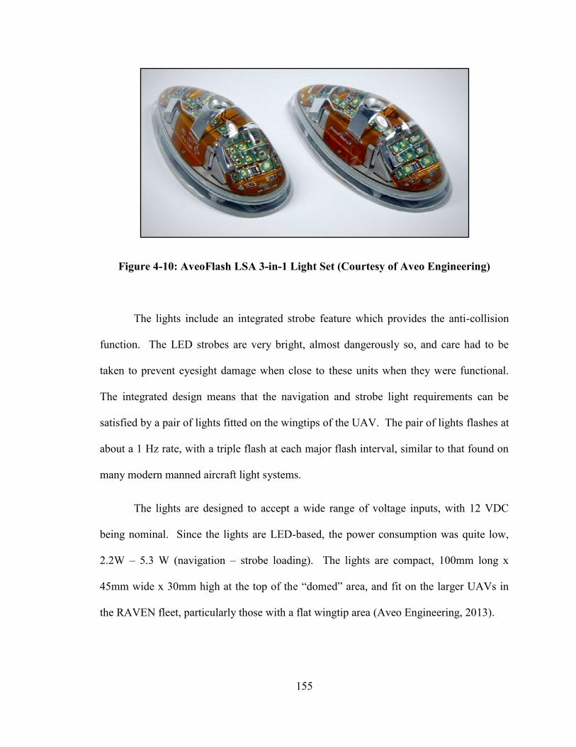
155
Figure 4-10: AveoFlash LSA 3-in-1 Light Set (Courtesy of Aveo Engineering)
The lights include an integrated strobe feature which provides the anti-collision
function. The LED strobes are very bright, almost dangerously so, and care had to be
taken to prevent eyesight damage when close to these units when they were functional.
The integrated design means that the navigation and strobe light requirements can be
satisfied by a pair of lights fitted on the wingtips of the UAV. The pair of lights flashes at
about a 1 Hz rate, with a triple flash at each major flash interval, similar to that found on
many modern manned aircraft light systems.
The lights are designed to accept a wide range of voltage inputs, with 12 VDC
being nominal. Since the lights are LED-based, the power consumption was quite low,
2.2W – 5.3 W (navigation – strobe loading). The lights are compact, 100mm long x
45mm wide x 30mm high at the top of the “domed” area, and fit on the larger UAVs in
the RAVEN fleet, particularly those with a flat wingtip area (Aveo Engineering, 2013).

156
4.2.1.3 Light Installation and Test Stand Apparatus
The light set was installed on the wingtips of a 3m (10ft) wing-set from a small
UAV. Wires were routed inside the wing-set and terminated using plugs to allow reliable
and safe connection to the power supply. A blue synchronization wire was used to
connect the pair of wingtip lights together, such that the strobe flashes were synchronized.
A custom-build wooden stand was available within the project, having been
constructed the year before for another purpose in the RAVEN Project. The wing set
was bolted onto the central “head” section, which also featured a pivot platform with
regular 22.5º interval azimuth settings pre-measured. This made the stand ideal for the
light experiment. The complete wing set setup, installed and powered at the end of the
main Argentia runway at dusk conditions, may be seen in Figure 4-11.
Figure 4-11: Night VFR Light Experiment Test Stand
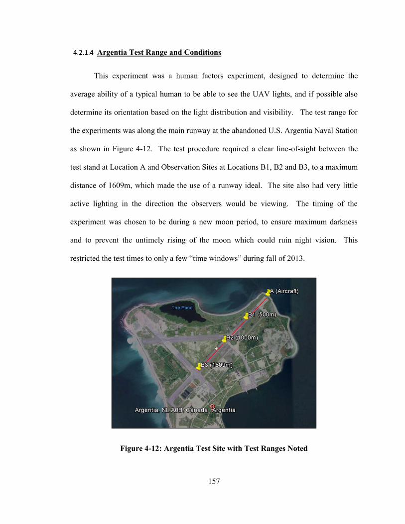
157
4.2.1.4 Argentia Test Range and Conditions
This experiment was a human factors experiment, designed to determine the
average ability of a typical human to be able to see the UAV lights, and if possible also
determine its orientation based on the light distribution and visibility. The test range for
the experiments was along the main runway at the abandoned U.S. Argentia Naval Station
as shown in Figure 4-12. The test procedure required a clear line-of-sight between the
test stand at Location A and Observation Sites at Locations B1, B2 and B3, to a maximum
distance of 1609m, which made the use of a runway ideal. The site also had very little
active lighting in the direction the observers would be viewing. The timing of the
experiment was chosen to be during a new moon period, to ensure maximum darkness
and to prevent the untimely rising of the moon which could ruin night vision. This
restricted the test times to only a few “time windows” during fall of 2013.
Figure 4-12: Argentia Test Site with Test Ranges Noted

158
4.2.1.5 Experimental Procedure
With the wing-set installed on the test stand and powered, the test operator at
Location A positioned the wing-set by turning it on the stand such that it presented
different azimuth view angles to observers at positions B1 through B3. Eight positions
were used as summarized in Table 4-4. The angles used followed the standard nautical
bearing sense (i.e. clockwise is positive, counter-clockwise negative).
Table 4-4: Wing-set Azimuth Positions Tested
Code Azimuth (deg) Descriptions
P1 0 Aircraft Pointing towards observation post (front view)
P2 45 Aircraft turning RIGHT at 45º relative to observation post
P3 90 Aircraft turning RIGHT at 90 º relative to observation post
P4 135 Aircraft turned RIGHT and heading away from observation
post at 45º
P5 180 Aircraft Pointing away from observation post (rear view)
P6 225 Aircraft turned LEFT and heading away from observation
post at 45º
P7 270 Aircraft turning LEFT at 90º relative to observation post
P8 315 Aircraft turning LEFT at 45º relative to observation post
At each of the Observation locations, tests subjects were brought inside the
darkened cab of a large Recreational Vehicle (RV), simulating night-time conditions in a
cockpit. After allowing vision to adjust to the dark conditions, the test sequence was
started. Five random positions were used for each test subject. The order was
randomized, and not all azimuth cases were tested for all subjects. Repeats of test points
were also possible. The idea was to present a completely random set of cases, and to
159
eliminate the possibility of test subjects guessing. Once each azimuth position adjustment
was done, the Test Operator at A communicated to the Operator at B in the cab that the
wing-set was “in position” and the subject was asked:
1) What lights can you see?
2) What is the orientation?
The correct determination of the relative direction of another aircraft at night,
based on the navigation lights visible, is an obvious safety consideration. This ability is
generally not an automatic one, but one learned by people in aviation or nautical fields,
both of which use the same conventions for navigation lights (i.e. red = left/port, green =
right/starboard). For this reason a visual aid was provided for the observers during the
experiment - a small UAV model with the position of the navigation lights shown – to
assist the observers.
The answers for each test subject were recorded by the Tester at location B, who
also did not know the order of the positions. In this way, any possibility of bias or “hints”
was reduced since neither the test subject nor Tester at B knew the real test orientations
being used at A.
This procedure was repeated for all test subjects. The RV was then moved further
down the runway to the next position, and the entire test sequence was repeated. This was
done until all test subjects were tested at all three observation positions:
1) B1 - 500m
2) B2 - 1000m
3) B3 – 1609m
160
The experiment was conducted on Saturday night, 5 October, 2013. The weather
at the start of the experiment was overcast, about 9ºC, with light winds (5 kts). A total of
thirteen (13) human test subjects arrived. The subjects had a good spread of ages (24 – 61
years), and a 5/8 split by gender (female/male). There was a blend of members from
Project RAVEN, significant others, plus a couple enlisted from the nearby community of
Placentia. A total of 65 observations were made at each of the three viewing ranges.
The first observations at B1 (500m) were conducted somewhat slowly as everyone
became accustomed to the test procedure. There were concerns about the late start (9:15
PM) and also the possibility of the weather deteriorating. It took a little over 1hr to
conduct the first set of tests. The results of each set of recordings will be summarized in
the next section. After this was completed, the RV was moved to the B2 (1000m)
location.
The second set of tests started at 10:30 PM. By this time, a light drizzle had
started, which hampered visibility out the window due to water droplets. However, the
lights on the wing-set were still visible, especially the strobe flashes. The windshield was
wiped frequently to keep the water droplets under control. However, this did cause delays
and resulted in the B2 series taking much longer. The RV was then moved to the final
B3 (1609m) location.
The third series was started at 12:15 AM. By this time the weather had cleared
and the drizzle which plagued the 1000m series had stopped. The temperature had dipped
161
and there was some concern about the health of the equipment and Operator at A.
However, both performed admirably, and the third set of observations were finally
completed at 1:30 AM. The human subjects were dismissed and the crew began the
teardown procedure at A which was completed by 2 AM.
4.2.1.6 Analysis of the Results
The results from the VFR Night-time Light experiment were analyzed to
determine the observation accuracy for all of the observers at each sighting distance.
While it is true that the sample size of the number of human subjects is small (13) the
total number of observations at each viewing location (65) does permit the determination
of overall trends in the results.
This first thing that was noted for all observers at all observation ranges and
viewing angles was that the strobe (flashing) of the wing-set lights were always visible.
This confirms the hypothesis that simply carrying a strobe, flashing at 1 Hz, immediately
makes the UAV easy to be spotted. The maximum range tested during the experiment
was 1609m. However, later observations from as far away as the lookout location
described in Chapter 3 (over 2.6 km away), confirmed the strobe was immediately
obvious at this range too. Thus, the addition of just the anti-collision strobe feature
should improve the chance that the small UAV would be spotted by human pilots, at least
out to a range of 2.6 km (1.6 mi).
The ability of the observers to determine the orientation of the aircraft (wing-set)
was also assessed, by comparing the observed position (what each person thought they

162
saw) against the actual position as recorded by the Operator at position A. To permit a
numerical accuracy to be calculated, the error in the observed positions versus the actual
position was calculated using these rules:
If observed position = actual, the accuracy is 100%
If observed position within +/-45º (i.e. one position step), accuracy is 75%
If observed position was off by +/-90º, accuracy is 50%
If observed position was off by +/-135º, accuracy is 25%
Worse than this was deemed to be an accuracy of 0%
The last rule represents the worst case scenario, where the observer has
misinterpreted the orientation by 180º (e.g. tail-on as a head-on situation).
The accuracy results are shown in Figure 4-13 for each of the three ranges B1
(500m), B2 (1000m) and B3 (1609m) in the form of polar plots. These summarize the
observation accuracy versus the real orientation of the wing-set as represented by the
Aerosonde UAV icon in the center (i.e. 0º = head-on, 90º = right side view, 180º =tail-on,
etc.). A mark on the outer circle indicates 100% accuracy, while a mark at the center
denotes 0% accuracy. The first three polar plots show the results sorted by gender. The
lower right is summary of all three observation ranges ignoring gender, plotted together to
permit a comparison.
There was almost no difference between genders in terms of observation accuracy.
The head-on and tail-on orientations were the easiest ones to be determine, generally at an

163
accuracy of 75% or better. The most difficult positions were the 45º off-axis positions,
especially those pointing away from the observer. These were the source of all of the 0%
accuracy results.
(B1) (B2)
(B3) (B123)
Figure 4-13: Position Interpretation Accuracy versus Viewing Angle at: (B1) 500m;
(B2) 1000m; (B3) 1609m; and, (B123) Comparison of all three ranges.
164
The results show a degradation of observation accurate with range, which was
expected. However, the degradation from 500m to 1000m is much worse than the step
from 1000m to 1609m. Indeed, the results appear to improve between the second and last
set of data. The drizzle during much of the 1000m observations likely deteriorated these
results. However, even in the face of adverse sighting conditions (i.e. rainy weather,
water on the windshield, etc.) the majority of the observations were still 50% accurate or
better at 1000m.
A surprising result is that even at 1609m, a full mile away, the majority of the
observations were able to distinguish the orientation of the aircraft, especially along the
cardinal directions (i.e. Front/Back and Left/Right). There were a few instances of
confusion over red/green versus left/right which may account for the lower accuracy at
270º azimuth (i.e. which is when the RED wing-tip was pointing towards us).
Therefore, even on a very small aircraft (i.e. 3m/10ft wingspan), the red/green wingtip
light method does appear to work, and the brightness and separation of the colours is still
sufficient to permit orientation to be determined.
4.2.2 Extended Range Observations
Unfortunately, time did not permit a check of the light visibility at longer ranges
on the same night as the VFR Night-time experiment. One month later during the next
new moon period, the Night VFR experiment setup was re-assembled in Argentia to
accomplish two tasks. First, still and video footage was recorded of the wing-set setup at
each of the three ranges B1 through B3. The original intent was to do these recordings at

165
the same time as the experiment. However, concerns over the safety of the delicate video
camera equipment in the wet weather (drizzle) prompted this step to be skipped. On the
night of November 5th
, the video recordings were conducted, though not without some
equipment failures due to the cold weather, including failure of a mounting system for the
hi-res video equipment which impacted the quality of the imagery obtained.
Next, the observing crew moved and re-assemble at the location of the lookout
area about 2.6 km away. From this vantage point, the lights on the wing-set were
immediately visible to the four people present, especially due to the distinct strobe pattern
used. This was how we were first able to locate the distant wing-set stand. When the
wing-set was rotated we could discern the change in orientation, but not based on the
ability to see individual points of light. Instead, the orientation could be determine as the
dominant colour of what appears as a fat single-point light source shifted from mostly
white, red/white, red/green together, green/white, then back to white again.
The ease by which we could locate the wing-set due to the strobe is very
important. We may conclude that as long as we are able to carry a strobe, it appears the
UAV would be visible at night in VMC conditions, at least 2.6 km away.
4.2.3 Daytime VFR Anti-Collision Light Testing
During the set-up of the light-stand both on the day of the night-time experiment
and the later set-ups for the video recordings, we were able to make observations of the
lighted wing-set during bright noon-hour conditions, mid-afternoon and about 1 hour
before dusk. It was noted that the coloured lights, especially the green, was very difficult
166
to see in full sunlight. However, the strobe flashes were still visible. Indeed, it was
usually by seeing the flashing lights that the eye was able to locate the position of the
wing-set against the busy background beyond the end of the runway. Predominantly this
was the ocean, and green forested terrain beyond. The inability to see the green light
made determining orientation difficult at 1000m, and impossible at 1609m. Orientation
could still be determined at 500m, by everyone in the crew (about 6 people) still located
at the GCS location.
As the light conditions started to dim, by around 4PM (i.e. 1 hour before sunset),
the coloured wingtip lights could now be seen quite clearly out to range of 1000m. But
determining the orientation at 1609m range was still very difficult, mostly due to sun
glare on the ocean surface beyond the end of the runway. However, just like in the
results from the Night-time observations, the flashing strobe pattern could always be seen.
4.2.4 Conclusions from Anti-Collision Light Experiments
Based on the results of the Night-time VFR experiment, and additional
observations both at day and night conditions, we may conclude the following concerning
the use of aviation lights on a small UAV:
1. The anti-collision strobe is easily spotted, particularly at night at least to a range of
2.6 km as tested. The brilliance of the strobe even at this range suggests that the
theoretical range limits calculated in Section 4.1 may be valid.
2. Determining the orientation of the small UAV appears possible out to at least 1.6
km based on the ability to see individual lights, but only during night-time VFR
conditions.
167
3. The limit of human vision acuity to discern distinct points of light at night is
estimated to be 4 arc-min. For our light set on a 3m (10ft) wing-set this
corresponds to a range of about 2.6 km, where the different lights merge together
to form a single point source. Our observations from 2.6 km validate this
theoretical estimate.
4. The ability to see the red or green wing-tip lights in conditions of full sunlight is
limited, perhaps only to a maximum range of 500m.
5. Equipping a small UAV with an anti-collision strobe should allow it to be detect at
least 2.6 km away during night, and also up to 1.6km away during the day.
4.3 An Equivalent UAV Vision Capability
Assuming we wish to equip the small UAV with a machine vision system that at
least matches the capabilities of a human pilot we could write the following requirements.
4.3.1 Visual Acuity
The vision system should have the following minimum visual detection capabilities:
1. Shall be able to detect a Cessna-size aircraft at a minimum range of 1609m (1 mi)
assuming Daytime VMC conditions.
2. Shall be able to detect anti-collision lights in Night-time VMC conditions at a
minimum of 3.2km (2 mi), and resolve wingtip navigation lights separated 3m at a
range of 1.6 km.
3. Shall have an instantaneous FOV of 60º. This would be a central conical area 30º
wide (15º half angle) with very high resolution equivalent to 4500 pixels wide (i.e.
15.9 million pixels in a circular region). The remaining area can be equivalent to
NTSC resolution.
4.3.2 Field of View and Scanning Ability
The vision system should have the following minimum FOV and scanning abilities:

168
1. Shall have a minimum Field of Regard (FOR) of +/- 110º horizontal and +/-15º
vertically.
2. Shall scan the entire range of azimuth and elevation angles at least once every 10
seconds.
4.3.3 Better than Human Vision Abilities
By meeting the above requirements, the UAV vision system would be equivalent
to a very consistent and perceptive human pilot. However, simply matching human pilot
visual capabilities is not sufficient, given the acknowledged limitations of normal human
vision. A better option may be to reduce the guaranteed detection range (e.g. to 1000m)
while giving the UAV the equivalent of HD resolution capability but with a full 360º FOR
in the horizontal plane. A vertical FOR of +/-30º should also be possible. This could be
implemented by a camera with a 60º FOV, using a fast rotating scan to sweep through
360º of azimuth. Such a vision system would exceed any human pilot in terms of
situational awareness in VFR conditions, in particular the ability to detect collision threats
approaching from behind.
4.4 Transponder Technologies
Transponders can be a very effective way to alert cooperative airspace users of
each other’s presence. The Mode-C, or altitude reporting version is the preferred type in
this role, especially to prevent mid-air collisions. If the transponder is also Mode-S
compliant it will also respond to TCAS interrogations. Transponders allow ATC to
monitor the location of each aircraft within their control zone, assuming the transponder is
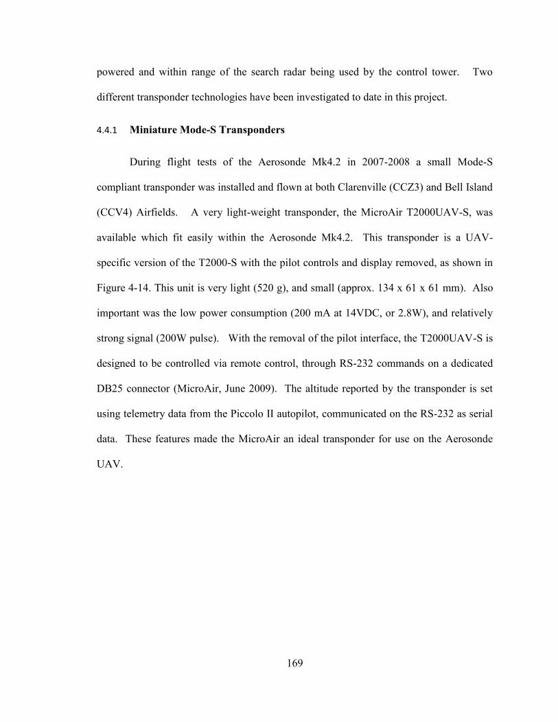
169
powered and within range of the search radar being used by the control tower. Two
different transponder technologies have been investigated to date in this project.
4.4.1 Miniature Mode-S Transponders
During flight tests of the Aerosonde Mk4.2 in 2007-2008 a small Mode-S
compliant transponder was installed and flown at both Clarenville (CCZ3) and Bell Island
(CCV4) Airfields. A very light-weight transponder, the MicroAir T2000UAV-S, was
available which fit easily within the Aerosonde Mk4.2. This transponder is a UAV-
specific version of the T2000-S with the pilot controls and display removed, as shown in
Figure 4-14. This unit is very light (520 g), and small (approx. 134 x 61 x 61 mm). Also
important was the low power consumption (200 mA at 14VDC, or 2.8W), and relatively
strong signal (200W pulse). With the removal of the pilot interface, the T2000UAV-S is
designed to be controlled via remote control, through RS-232 commands on a dedicated
DB25 connector (MicroAir, June 2009). The altitude reported by the transponder is set
using telemetry data from the Piccolo II autopilot, communicated on the RS-232 as serial
data. These features made the MicroAir an ideal transponder for use on the Aerosonde
UAV.
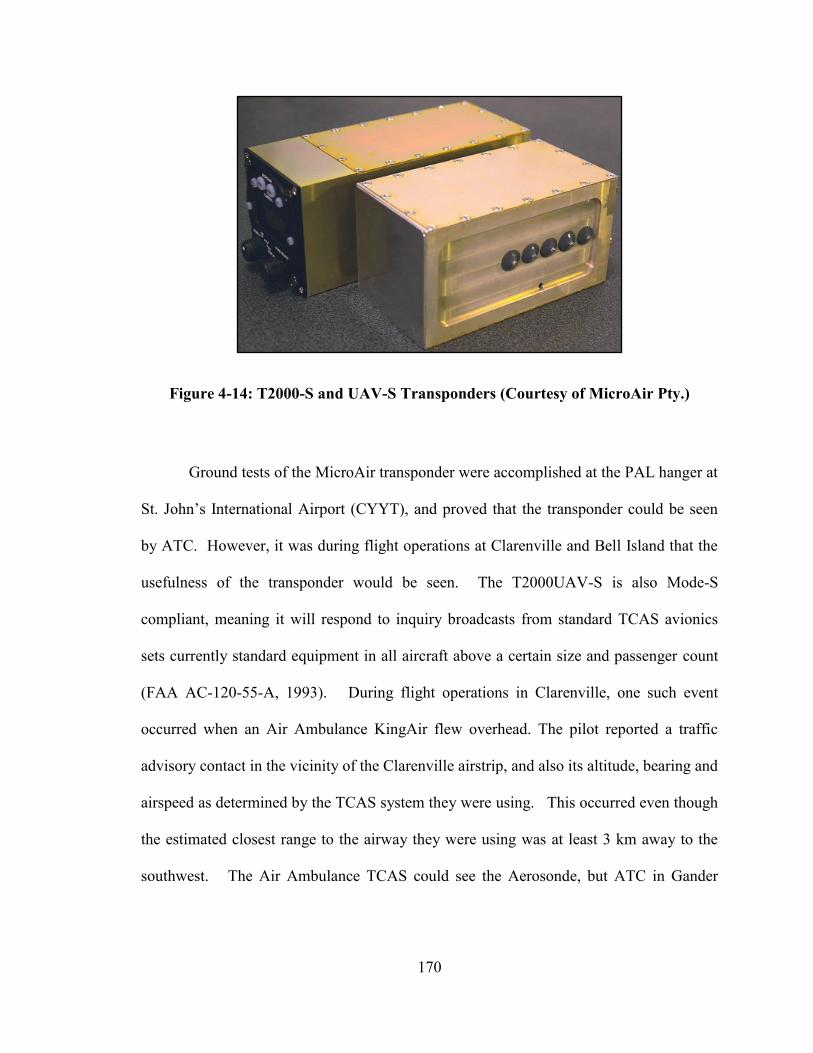
170
Figure 4-14: T2000-S and UAV-S Transponders (Courtesy of MicroAir Pty.)
Ground tests of the MicroAir transponder were accomplished at the PAL hanger at
St. John’s International Airport (CYYT), and proved that the transponder could be seen
by ATC. However, it was during flight operations at Clarenville and Bell Island that the
usefulness of the transponder would be seen. The T2000UAV-S is also Mode-S
compliant, meaning it will respond to inquiry broadcasts from standard TCAS avionics
sets currently standard equipment in all aircraft above a certain size and passenger count
(FAA AC-120-55-A, 1993). During flight operations in Clarenville, one such event
occurred when an Air Ambulance KingAir flew overhead. The pilot reported a traffic
advisory contact in the vicinity of the Clarenville airstrip, and also its altitude, bearing and
airspeed as determined by the TCAS system they were using. This occurred even though
the estimated closest range to the airway they were using was at least 3 km away to the
southwest. The Air Ambulance TCAS could see the Aerosonde, but ATC in Gander

171
could not, as we were well beyond the range of the Gander search radar, especially given
the terrain between Gander and Clarenville. However Gander ATC was aware of our
presence at Clarenville due to the SFOC and Notice to Airmen (NOTAM) we had filed,
and advised the Air Ambulance pilot of our experimental UAV operations.
During a second series of flight tests at Bell Island on June 18, 2008, a
transponder-equipped Aerosonde was flown over the airstrip, which is located on the
northwest coast of the island. We were located about 2km north of the approach path to
Runway 11 at St. John’s International Airport, flying well below (i.e. under 365m/1200ft)
so we would not conflict with air traffic on this approach vector. The weather conditions
were such that this was the approach being used at around noon, when several
commercial aircraft flew overhead. Each reported a TCAS traffic advisory, similar to the
experience of the Air Ambulance pilot in Clarenville. Since we were monitoring using
an Air band radio, a requirement since we were using an active runway on Bell Island, we
were able to hear both the pilot and ATC exchanges concerning these TCAS events. One
typical exchange was that of an Air Canada A319 captain:
Pilot: “Torbay tower this is AC flight xxx, reporting TCAS contact at our 11 o’clock…
VERY low…around sea level…going 50 knots…..please advise…”
Tower: “…Roger AC flight xxx….that is experimental UAV flying at Bell Island
runway…”
Pilot: “….Roger…didn’t know these could be seen on traffic advisory…very good…it’s
tracking them pretty good…”
172
Similar exchanges were noted with a WestJet B737 and an Air Labrador Dash-8
also landing on Runway 11. What is key is all of these aircraft could see the Aerosonde
on their TCAS systems, and all reported what must have appeared as a very strange
contact (i.e. a 50 knot aircraft at sea level!). We can conclude that the “professional”
flyers, especially the larger passenger planes which must use TCAS, are able to see our
UAV if equipped with a Mode-S compliant transponder like the MicroAir T2000UAV-S,
and at a significant range (i.e. at least 3 km).
4.4.2 Automatic Dependent Surveillance-Broadcast Transponders
RAVEN has also been experimenting with the use of ADS-B transponders as
another method for cooperative aircraft traffic de-confliction and collision avoidance.
Each ADS-B avionics set determines its own position using GPS, and broadcasts this
information using 1040 or 975 MHz (these two bands are proposed for larger aircraft, or
smaller types which fly below 6000 m (18,000 ft), respectively). All ADS-B receivers in
range are therefore able to determine the location of all other similarly-equipped aircraft.
It is proposed in the U.S. to replace the present transponder-based air traffic control
system with the ADS-B based method by 2020 (Federal Aviation Administration (FAA),
2010). The ADS-B system also allows other information to be received, including
weather, terrain, NOTAM/Advisory information and also position information sent by
ATC for aircraft whose location is known via other means (e.g. traditional transponders or
search radars). This last data-fusion capability remains an active research area in the
follow-on research activities after Project RAVEN.
173
4.5 Air-band Radios
A technology that has overlooked for UAVs is the provision of a two-way radio
communication capability. For manned aircraft, two-way radio communications with
other aircraft, and between aircraft and ATC, are major contributors to the situational
awareness of each pilot who share the same radio channels. The ability to be able to hear
status and position reports, and also the stated intentions of each pilot, especially close to
busy airports, is cited in VFR and IFR regulations as a major requirement and is a
contributor to the overall flight safety regime (MacDonald & Peppler, 2000). The
inability of pilots to communicate with the “blind and dumb” UAV is a common
complaint against them (Kirkby, 2006).
It is proposed that all UAVs should be given the ability to communicate their
status and intentions to other users of the airspace, and ATC, in a manner exactly like the
regular radio calls that are the standard practise in manned aviation (RMC Inc.). This
capability could take the form of the UAV acting as a relay station to the GCS. The AVO
would then assume the role of the manned pilot, communicating with ATC and the other
aircraft using the same standard language and following standard radio call procedures. If
this method is used, every AVO would have to be trained and certified in the use of
aviation air-band radios, or hold the equivalent of a GA pilot license (MacDonald &
Peppler, p. 217).
An alternative form of this communication capability could be an autonomous
two-way communication channel centered on the UAV. The UAV could be programmed

174
to respond automatically when it detects another aircraft in the vicinity, or if it detects it
has entered a controlled airspace zone. The automatic response could be triggered by a
TCAS or ADS-B query, radar/transponder sweeps, or when the channel detects a message
directed at itself (i.e. assuming the use of a unique call sign similar to manned aircraft).
This would require some form of speech recognition and artificial intelligence to ensure
the UAV “voice” responds properly. This autonomous mode would be most effective
when the UAV is flying in very remote locations outside the range of any GCS.
4.6 Summary: Impact of Visibility Enhancements on Safety
Without some form of visibility enhancements, it is unlikely that small UAVs
would be visible to manned aircraft at anywhere near the normal sighting distances
implied in aviation regulations. Theoretical estimates suggest that a small UAV such as
the Aerosonde is unlikely to be spotted until it is less than 500m away under ideal
daylight lighting conditions.
With the addition of an anti-collision strobe, night-time visibility should improve
when VFR conditions prevail. Based on night-time observations, the strobe should be
visible at 2.6 km range or more. During daylight conditions, observations indicate the
strobe would still be visible up to 1.6 km away. Therefore, the Estimated Level of Safety
of the small UAV could be improved simply by it carrying a set of aviation-grade lights,
in particular an anti-collision strobe. This would improve the chances that a manned
aircraft might spot the small UAV with sufficient warning to avoid traffic conflicts and

175
reduce the probability of a mid-air collision. This would apply whether or not the other
aircraft is co-operative (i.e. using a transponder), but only in visual flying conditions.
If the small UAV is equipped with a small Mode-S Transponder (i.e. one
compliant with TCAS interrogation protocols), it will become visible to both ATC and
any aircraft nearby equipped with TCAS. The range of detection has been demonstrated
to be a minimum of 3 km. The range for detection by ATC has not been measured
rigorously but should be at least this range or better, especially given the improved
sensitivity of the ground-based receive antennas used by the control towers at major
airports. ADS-B may have a similar effect, but only in a cooperative DSA environment.
Unlike the light system, these transponder-based enhancements will work in non-visual
(IFR) conditions. If combined with the TCAS functionality, detection of the small UAV
should be automatic at the 3 km range. This would greatly reduce the risk of mid-air
collision, especially in controlled airspace.
Equipping the small UAV with a two-way radio would be a simple but important
enhancement to safety, simply by enhancing the situational awareness of all pilots and
ATC in the area of the UAV presence and intentions. This may also have the beneficial
impact of improving the perception of the UAV amongst pilots, who might start to regard
the UAV as a cooperative member of the airspace community.
176
Chapter 5 4D Simulations and Avoidance Maneuvers
The topic of DSA related to UAVs naturally leads to the subject of 4D maneuvers.
4D maneuvers refer to two UAVs which are synchronized in both space and time in such
a way that they encounter each other (i.e. 3D space plus time or 4D). The ability to create
a rich set of repeatable 4D maneuvers is crucial for enabling the collection of realistic air-
to-air data which may be used to develop DSA sensors and strategies. They are also a
means to conduct validation testing of any hypothetical DSA method. But setting up 4D
encounters is not easy. In this chapter a simulation environment will be described which
may be used to develop 4D maneuver flight-plans and DSA before committing to
expensive field testing until confident they will work. A discussion of typical 4D
maneuvers will follow, including an introduction to an improved 4D maneuver method.
Finally, assuming a collision threat is detected, what avoidance maneuvers are possible
for either the manned aircraft or small UAV? Is such an avoidance maneuver the best
option and what form should it take?
5.1 4D Encounter Simulation Environment
An aerodynamic simulation environment has been developed which permits the
simulation of dual-UAV encounter scenarios in real-time. This section will describe in
detail how this simulation was developed, the mathematical basis for the simulation and
the enhanced features recently added to support 4D simulations.

177
5.1.1 Historical Background
The current simulation environment is the result of over 8 years of development.
The simulation has evolved greatly and has been used for many different purposes. It
was originally developed as a mission simulation and planning tool to simulate typical
ship inspection scenarios by small UAVs in the Newfoundland offshore environment
(2005-2006). The simulation started as an enhancement of a demo simulation included in
the original AeroSIM toolkit for MATLAB/Simulink (Unmanned Dynamics, 2006). The
original visualization method used the Microsoft Flight Simulator 2004. However, poor
real-time performance and the closed nature of this commercial product limited the
possibilities of customizing the simulation. The visualization method was switched to
FlightGear (FG), a free open-source flight simulator. A key feature of FG was that it
permitted the use of an external simulation to drive the Flight Dynamics Model (FDM).
Even at this early stage of development, the MATLAB/Simulink simulation was able to
drive the FG visual display on the same computer, as shown in Figure 5-1, with
reasonable performance. This method could also be used to send FDM across the
internet to a remote PC running the visualization tool (FG). The simulation also included
a rudimentary autopilot simulation which could control the UAV heading, speed and
airspeed. This was used to simulate typical off-shore inspection maneuvers, involving
orbiting a moving ground target (i.e. ship) at typical distances of 300-500 m.
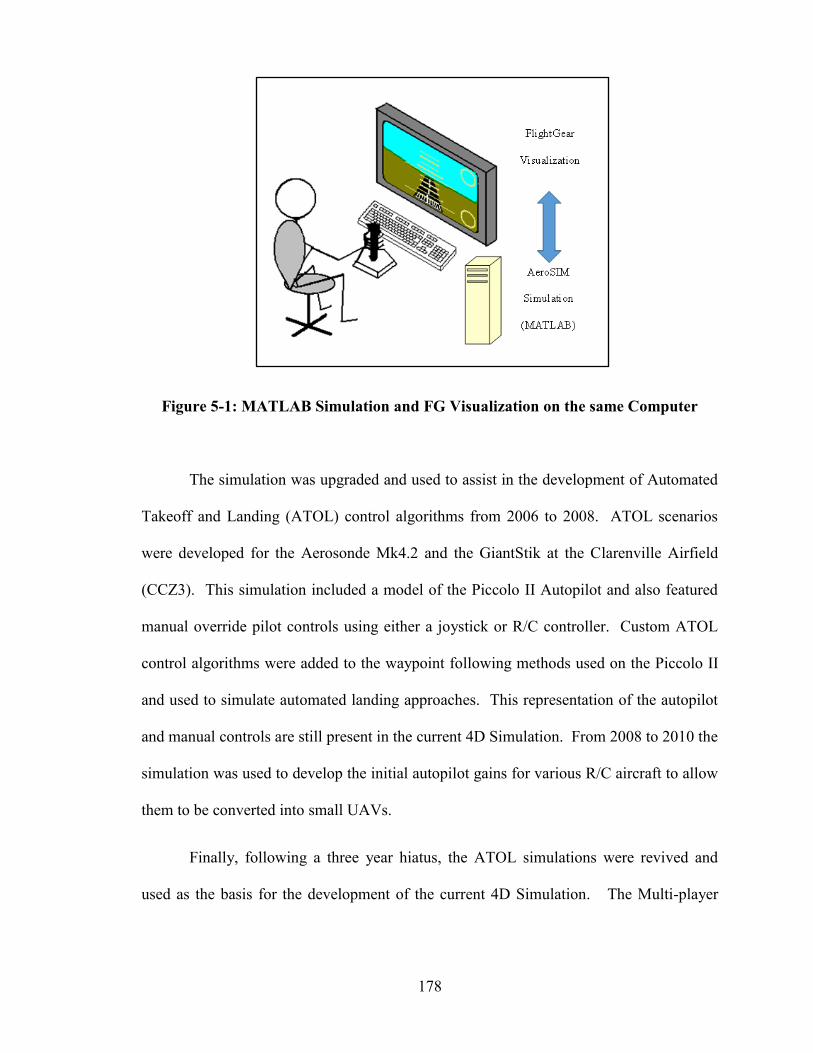
178
Figure 5-1: MATLAB Simulation and FG Visualization on the same Computer
The simulation was upgraded and used to assist in the development of Automated
Takeoff and Landing (ATOL) control algorithms from 2006 to 2008. ATOL scenarios
were developed for the Aerosonde Mk4.2 and the GiantStik at the Clarenville Airfield
(CCZ3). This simulation included a model of the Piccolo II Autopilot and also featured
manual override pilot controls using either a joystick or R/C controller. Custom ATOL
control algorithms were added to the waypoint following methods used on the Piccolo II
and used to simulate automated landing approaches. This representation of the autopilot
and manual controls are still present in the current 4D Simulation. From 2008 to 2010 the
simulation was used to develop the initial autopilot gains for various R/C aircraft to allow
them to be converted into small UAVs.
Finally, following a three year hiatus, the ATOL simulations were revived and
used as the basis for the development of the current 4D Simulation. The Multi-player
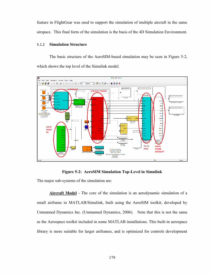
179
feature in FlightGear was used to support the simulation of multiple aircraft in the same
airspace. This final form of the simulation is the basis of the 4D Simulation Environment.
5.1.2 Simulation Structure
The basic structure of the AeroSIM-based simulation may be seen in Figure 5-2,
which shows the top level of the Simulink model.
Figure 5-2: AeroSIM Simulation Top-Level in Simulink
The major sub-systems of the simulation are:
Aircraft Model - The core of the simulation is an aerodynamic simulation of a
small airframe in MATLAB/Simulink, built using the AeroSIM toolkit, developed by
Unmanned Dynamics Inc. (Unmanned Dynamics, 2006). Note that this is not the same
as the Aerospace toolkit included in some MATLAB installations. This built-in aerospace
library is more suitable for larger airframes, and is optimized for controls development

180
work. The AeroSIM library from Unmanned Dynamics was developed specifically to
allow the simulation of smaller aircraft, in particular UAVs like the Aerosonde or small
R/C type aircraft (Unmanned Dynamics, 2006). The mathematical basis of this aircraft
model is provided in the next section.
Autopilot - This is a representation of the Piccolo II autopilot, which will be
described only at a very high level here. A detailed description is provided in Appendix
E. Outer Loop control loops are used to calculate speed, heading and altitude commands.
The nominal waypoint following method defines these based on the range and distance to
the next waypoint. Additional modes include waypoint orbit and simulated active
guidance to a target. The Outer Loop commands are used to drive a set of Inner Loops.
These Inner Loops are PID-based control loops which control the pitch, yaw, roll, altitude
and velocity needed to achieve the Outer Loop commands, by manipulating the flight
surfaces (elevator, aileron, rudder and flaps) and engine throttle settings. The outputs
from the Autopilot are feed to the Aircraft Model block which includes detailed models of
the effects from the flight surfaces and throttle setting. The manual control overrides are
located just underneath the Autopilot and are direct inputs of the flight surfaces and
throttle settings, which may come from a standard R/C controller or a joystick.
Inputs from FG – This is an AeroSIM interface module which allows the
interception of FG output information. This is used in the current simulation to return the
ground altitude obtained from the FG terrain mesh. This is used for ATOL control
modes.
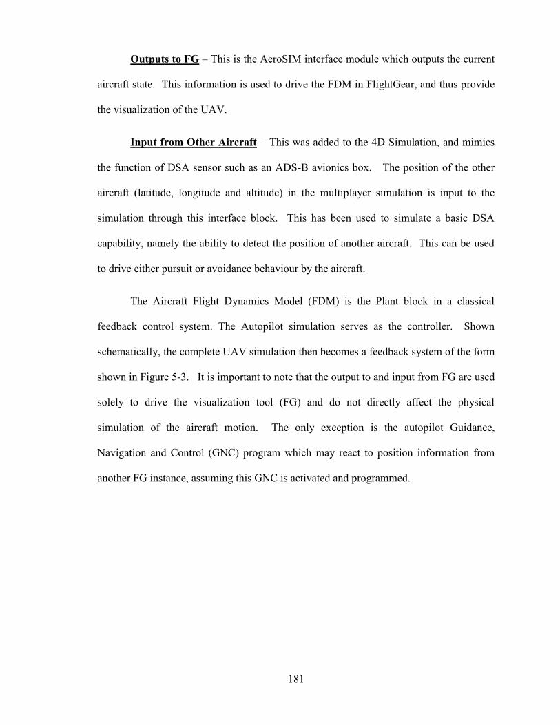
181
Outputs to FG – This is the AeroSIM interface module which outputs the current
aircraft state. This information is used to drive the FDM in FlightGear, and thus provide
the visualization of the UAV.
Input from Other Aircraft – This was added to the 4D Simulation, and mimics
the function of DSA sensor such as an ADS-B avionics box. The position of the other
aircraft (latitude, longitude and altitude) in the multiplayer simulation is input to the
simulation through this interface block. This has been used to simulate a basic DSA
capability, namely the ability to detect the position of another aircraft. This can be used
to drive either pursuit or avoidance behaviour by the aircraft.
The Aircraft Flight Dynamics Model (FDM) is the Plant block in a classical
feedback control system. The Autopilot simulation serves as the controller. Shown
schematically, the complete UAV simulation then becomes a feedback system of the form
shown in Figure 5-3. It is important to note that the output to and input from FG are used
solely to drive the visualization tool (FG) and do not directly affect the physical
simulation of the aircraft motion. The only exception is the autopilot Guidance,
Navigation and Control (GNC) program which may react to position information from
another FG instance, assuming this GNC is activated and programmed.
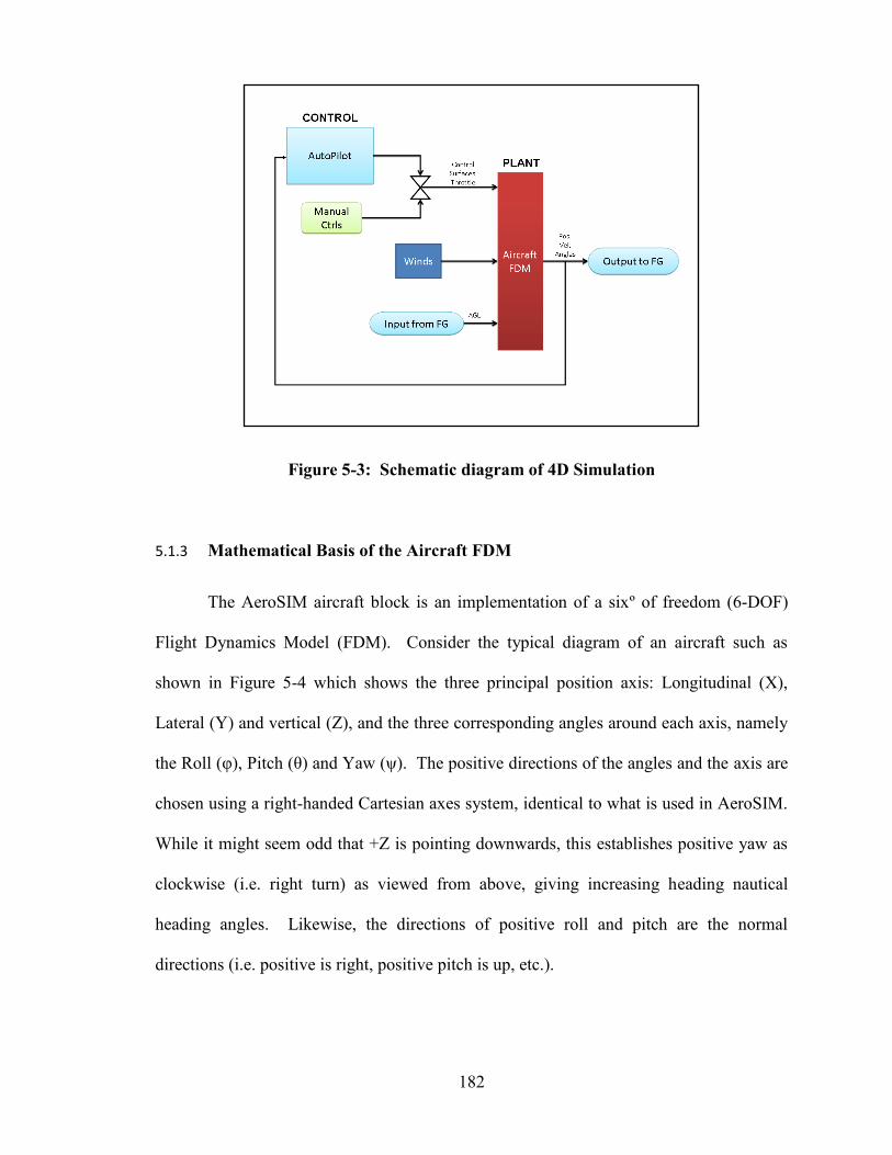
182
Figure 5-3: Schematic diagram of 4D Simulation
5.1.3 Mathematical Basis of the Aircraft FDM
The AeroSIM aircraft block is an implementation of a sixº of freedom (6-DOF)
Flight Dynamics Model (FDM). Consider the typical diagram of an aircraft such as
shown in Figure 5-4 which shows the three principal position axis: Longitudinal (X),
Lateral (Y) and vertical (Z), and the three corresponding angles around each axis, namely
the Roll (φ), Pitch (θ) and Yaw (ψ). The positive directions of the angles and the axis are
chosen using a right-handed Cartesian axes system, identical to what is used in AeroSIM.
While it might seem odd that +Z is pointing downwards, this establishes positive yaw as
clockwise (i.e. right turn) as viewed from above, giving increasing heading nautical
heading angles. Likewise, the directions of positive roll and pitch are the normal
directions (i.e. positive is right, positive pitch is up, etc.).
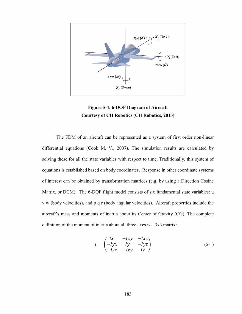
183
Figure 5-4: 6-DOF Diagram of Aircraft
Courtesy of CH Robotics (CH Robotics, 2013)
The FDM of an aircraft can be represented as a system of first order non-linear
differential equations (Cook M. V., 2007). The simulation results are calculated by
solving these for all the state variables with respect to time. Traditionally, this system of
equations is established based on body coordinates. Response in other coordinate systems
of interest can be obtained by transformation matrices (e.g. by using a Direction Cosine
Matrix, or DCM). The 6-DOF flight model consists of six fundamental state variables: u
v w (body velocities), and p q r (body angular velocities). Aircraft properties include the
aircraft’s mass and moments of inertia about its Center of Gravity (CG). The complete
definition of the moment of inertia about all three axes is a 3x3 matrix:
𝐼 = (
𝐼𝑥 −𝐼𝑥𝑦 −𝐼𝑥𝑧−𝐼𝑦𝑥 𝐼𝑦 −𝐼𝑦𝑧−𝐼𝑧𝑥 −𝐼𝑧𝑦 𝐼𝑧
) (5-1)

184
The signs are used to preserve the right-hand coordinate system centered on the
aircraft CG. For most aircraft, symmetry and uniform distribution of mass about the x-z
plane can be assumed, so the products of inertia may be assumed to be zero (i.e. Ixy = Iyx
= Izy = Iyz = 0). Since Ixz and Izx are generally very small for a symmetrical body, we
may also assume that Ixz = Izx = 0. The linear accelerations along the three principle
axes can be expressed as follows (Cook M. V., 2007):
�̇� = 𝑟𝑣 − 𝑞𝑤 + ∑ 𝐹𝑥/𝑚 (5-2)
�̇� = 𝑝𝑤 − 𝑟𝑢 + ∑ 𝐹𝑦/𝑚 (5-3)
�̇� = 𝑞𝑢 − 𝑝𝑣 + ∑ 𝐹𝑧/𝑚 (5-4)
Where u, v and w are the linear velocities along the x, y and z axes. Likewise, r,
p, q are angular velocities about the x, y and z axes. Fx, Fy, and Fz are total forces along
each axis. m is the mass of the vehicle. In the AeroSIM model, mass is calculated at
each time step, starting with the empty mass plus the current mass of the fuel tank. As
fuel is consumed, the mass of the fuel tank and the overall vehicle mass will decrease.
There will also be a slight shift of the CG position fore or aft, depending on where the
fuel tank position is defined. Note that this only applies to fuel-driven aircraft. For
electric-powered aircraft, mass is held constant, and these adjustments are un-necessary.
The angular accelerations about the three axes can be expressed as (Cook M. V.,
2007):
�̇� = [∑ 𝑀𝑥 + (𝐼𝑦 − 𝐼𝑧)𝑞𝑟]/𝐼𝑥 (5-5)
�̇� = [∑ 𝑀𝑦 + (𝐼𝑥 − 𝐼𝑧)𝑝𝑟]/𝐼𝑦 (5-6)

185
�̇� = [∑ 𝑀𝑧 + (𝐼𝑥 − 𝐼𝑦)𝑝𝑞]/𝐼𝑧 (5-7)
The moment terms take into account the instantaneous sums of these moments
about the aircraft CG in all three axes. This includes the effect of the aerodynamic
loadings on the various parts of the aircraft, in particular the main wing, fuselage and tail
surfaces. In all cases standard non-dimensional aerodynamic coefficients, in particular
the Lift (CL), Drag (CD) and Moment Coefficients (Cm) are calculated as functions of
the appropriate angles. All three angular conditions are considered, and not just pitch.
The effect of roll, pitch and yawing moments are calculated from the appropriate moment
coefficients based on how the body is moving through the airstream (i.e. the actual body
angles versus perfect alignment with the free stream velocity). The effect of the control
surfaces are included as deltas on these nominal moment coefficients, which generally
increase as a function of how far the control surface has rotated. The effect of the throttle
setting is also included, and is used to set the propeller rotational speed. Propeller speed
ultimately translates into a thrust, primarily along the longitudinal axis of the aircraft and
thus mostly affecting the Fx term in equation 5-2. The effect of off-axis and side-thrust
are included, to account for off-axis propeller line of force, which is common in single
engine propeller aircraft.
The rates of change of the roll, pitch and yaw angles may be calculated as follows
(Mathworks, 2007):
�̇� = 𝑝 + (𝑞 sin 𝜙 + 𝑟 𝑐𝑜𝑠𝜙)𝑠𝑖𝑛𝜃/𝑐𝑜𝑠𝜃 (5-8)
�̇� = 𝑞 cos 𝜙 − 𝑟 𝑠𝑖𝑛𝜙 (5-9)
�̇� = (𝑞 sin 𝜙 + 𝑟 𝑐𝑜𝑠𝜙)/𝑐𝑜𝑠𝜃 (5-10)
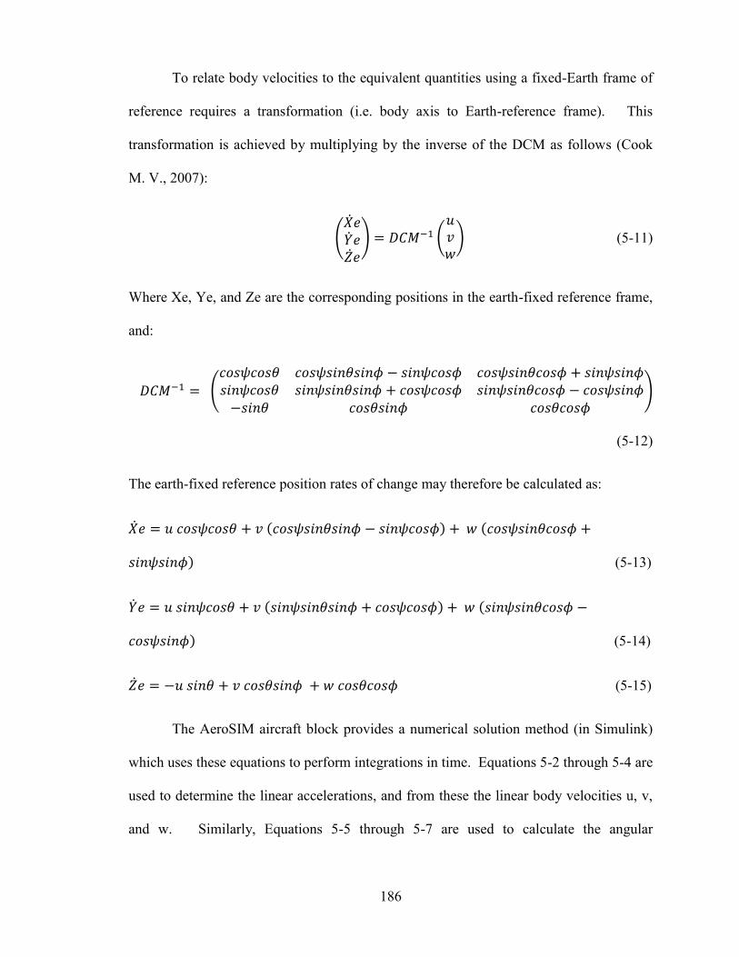
186
To relate body velocities to the equivalent quantities using a fixed-Earth frame of
reference requires a transformation (i.e. body axis to Earth-reference frame). This
transformation is achieved by multiplying by the inverse of the DCM as follows (Cook
M. V., 2007):
(�̇�𝑒�̇�𝑒�̇�𝑒
) = 𝐷𝐶𝑀−1 (𝑢𝑣𝑤
) (5-11)
Where Xe, Ye, and Ze are the corresponding positions in the earth-fixed reference frame,
and:
𝐷𝐶𝑀−1 = (
𝑐𝑜𝑠𝜓𝑐𝑜𝑠𝜃 𝑐𝑜𝑠𝜓𝑠𝑖𝑛𝜃𝑠𝑖𝑛𝜙 − 𝑠𝑖𝑛𝜓𝑐𝑜𝑠𝜙 𝑐𝑜𝑠𝜓𝑠𝑖𝑛𝜃𝑐𝑜𝑠𝜙 + 𝑠𝑖𝑛𝜓𝑠𝑖𝑛𝜙𝑠𝑖𝑛𝜓𝑐𝑜𝑠𝜃 𝑠𝑖𝑛𝜓𝑠𝑖𝑛𝜃𝑠𝑖𝑛𝜙 + 𝑐𝑜𝑠𝜓𝑐𝑜𝑠𝜙 𝑠𝑖𝑛𝜓𝑠𝑖𝑛𝜃𝑐𝑜𝑠𝜙 − 𝑐𝑜𝑠𝜓𝑠𝑖𝑛𝜙
−𝑠𝑖𝑛𝜃 𝑐𝑜𝑠𝜃𝑠𝑖𝑛𝜙 𝑐𝑜𝑠𝜃𝑐𝑜𝑠𝜙)
(5-12)
The earth-fixed reference position rates of change may therefore be calculated as:
�̇�𝑒 = 𝑢 𝑐𝑜𝑠𝜓𝑐𝑜𝑠𝜃 + 𝑣 (𝑐𝑜𝑠𝜓𝑠𝑖𝑛𝜃𝑠𝑖𝑛𝜙 − 𝑠𝑖𝑛𝜓𝑐𝑜𝑠𝜙) + 𝑤 (𝑐𝑜𝑠𝜓𝑠𝑖𝑛𝜃𝑐𝑜𝑠𝜙 +
𝑠𝑖𝑛𝜓𝑠𝑖𝑛𝜙) (5-13)
�̇�𝑒 = 𝑢 𝑠𝑖𝑛𝜓𝑐𝑜𝑠𝜃 + 𝑣 (𝑠𝑖𝑛𝜓𝑠𝑖𝑛𝜃𝑠𝑖𝑛𝜙 + 𝑐𝑜𝑠𝜓𝑐𝑜𝑠𝜙) + 𝑤 (𝑠𝑖𝑛𝜓𝑠𝑖𝑛𝜃𝑐𝑜𝑠𝜙 −
𝑐𝑜𝑠𝜓𝑠𝑖𝑛𝜙) (5-14)
�̇�𝑒 = −𝑢 𝑠𝑖𝑛𝜃 + 𝑣 𝑐𝑜𝑠𝜃𝑠𝑖𝑛𝜙 + 𝑤 𝑐𝑜𝑠𝜃𝑐𝑜𝑠𝜙 (5-15)
The AeroSIM aircraft block provides a numerical solution method (in Simulink)
which uses these equations to perform integrations in time. Equations 5-2 through 5-4 are
used to determine the linear accelerations, and from these the linear body velocities u, v,
and w. Similarly, Equations 5-5 through 5-7 are used to calculate the angular
187
accelerations which are integrated to determine p, q and r. The change of the body
angles are then calculated using equations 5-8 through 5-10. Equations 5-13 through 5-15
are used to calculate the corresponding change in the aircraft position in terms of the
fixed-earth.
Once the body velocities are known, the angle of attack α, and side-slip angle β,
both which are critical to determining the aerodynamic coefficients, may be determined
from basic trigonometry:
tan 𝛼 = 𝑤
𝑢 (5-16)
sin 𝛽 =𝑣
√𝑢2+𝑣2+𝑤2 (5-17)
Simulink integrates the FDM mathematics for each time step, marching forward in
time. The size of this time step is critical, as it needs to be fine enough for numerical
stability. However, if the time step is too small, the ability to simulate the aircraft in real-
time is limited. For the small UAVs being simulated in this project, a base time step of
10 ms using the Runge-Kutta (ode4) integration method gave a good compromise
between simulation stability and accuracy while still allowing the simulation to run in
real-time.
5.1.4 4D Encounter Simulations using Multiplayer
The multiplayer feature built-in to FlightGear was intended to allow users to
experience the realism of flying an aircraft in an environment shared by other aircraft
(FlightGear, 2010). The FlightGear multiplayer method uses internet protocol ports to
output the local aircraft FDM data to a remote server. A corresponding input port is used
188
to accept FDM data for any other aircraft in the local area of the user’s aircraft. FG has
limits on what will be displayed based on range, centered on the current view. Usually
this is the forward cockpit view, but could also be a tower view or other external view
like a chase plane view, all which are typically near the local aircraft. The range limit for
most aircraft in FG is 5000m (5 km), though this is also user-configurable in each aircraft
definition file. Several international server sites have been created to support the FG
Multiplayer mode.
Given the open source nature of FG, it was determined that any computer could be
used as a server, requiring only that the internet protocol (IP) address be known by the
other computer(s). An experiment was conducted where the server address for computer
1 was defined as that of a second nearby computer 2. Likewise, the server address for
computer 2 was set to that of computer 1. Once the right port numbers were assigned the
experiment was successful and the two aircraft could see each other. The external views
on both FG instances also showed both aircraft existing simultaneously on each of the FG
visualizations.
Each computer was then setup to host one instance of the MATLAB simulation,
and a local instance of FG as the visualization tool. This created a dual-computer 4D
simulation environment as shown in Figure 5-5.

189
Figure 5-5: Multiplayer-based 4D Simulation Environment
The UDP port numbers and IP addresses for each computer become the
corresponding remote settings for the other computer. For example, assuming the Target
PC has an address of 192.168.2.11 while the Intruder PC has an address of 192.168.2.12,
the Multiplayer settings for each computer then become as shown in Table 5-1.
Table 5-1: FlightGear Multiplayer Internet Settings
Computer Local IP
Address
Multiplayer
Server IP
INPUT
PORT
OUTPUT
PORT
Target
UAV
192.168.2.11 192.168.2.12 5510 5520
Intruder
UAV
192.168.2.12 192.168.2.11 5520 5510
The FG multiplayer mode provides a stable simulation assuming a good internet
connection is maintained. This works across any two computers located anywhere in the
world with an internet connection. The method also works for laptops using a wireless
connection. However, connection problems were encountered when attempting to drive

190
the simulation on remote PCs where one was protected behind a network firewall. As
long as reasonably powerful computers are used, the simulations run in real-time.15
The
4D simulation environment provides a compelling visual test environment as shown in
Figure 5-6. In this example, an Aerosonde UAV has just crossed in front of the first
aircraft, travelling from right to left. This environment was used to develop typical 4D
encounter maneuvers as discussed in the next section.
Figure 5-6: Screen Capture of a typical simulated 4D Encounter
15 This simulation is fairly math-intensive. While a desktop or laptop can be used, The PC hardware must be able to run
both FlightGear and MATLAB simultaneously. For this reason the minimum processor should be a Centrino Duo or better, although
an i5 or better is preferred. The PC should also have a good amount of memory (1GB minimum for WinXp based, 4GB minimum for
Windows 7). The PC must also have good graphics capability to support the FlightGear visualization tool at high-resolution (i.e.
minimum of 1080x768, although 1280 x 800 is preferred).

191
5.2 Development of 4D Encounter Geometries
The creation of repeatable 4D encounter geometries is of obvious interest and
importance to anyone involved in the development of DSA technologies. In spite of the
concerns regarding the UAV as a collision threat, deliberately creating the hazardous
situation of one aircraft being on a collision course with another at a variety of encounter
angles, is not a trivial task.
5.2.1 Opposing Circuits
One of the simplest methods used to create 4D encounter scenarios, and a method
commonly used within Project RAVEN, is to use opposing circuits. This was the method
used during the ADS-B testing described in Chapter 4. In this method, one aircraft is
flown in a typical circuit, such that it flies down the center line of the runway once per
circuit. This is easily accomplished using a basic 4-waypoint autopilot flight-plan as
shown in Figure 5-7 in BLUE (i.e. ABCD). A second aircraft is now added, flying a
similar circuit but in the opposite direction (i.e. BADC) as shown in RED. Note that an
alternative method could be to define the second circuit as illustrated in GREEN.
However, assuming the manual pilots and GCS are located at the bottom edge of the
runway as noted, this GREEN flight-plan would involve one of the aircraft flying behind
the GCS every circuit. This is not normally done as it could pose a safety hazard. The
requirement that one of the manual pilots must now “pirouette” during every circuit also
becomes very tiresome. For these reasons the RED and BLUE patterns are more
typically used.
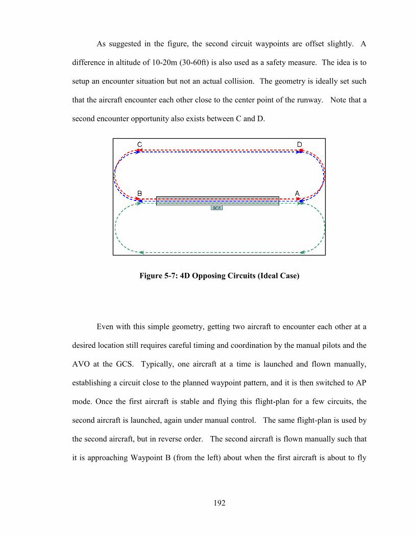
192
As suggested in the figure, the second circuit waypoints are offset slightly. A
difference in altitude of 10-20m (30-60ft) is also used as a safety measure. The idea is to
setup an encounter situation but not an actual collision. The geometry is ideally set such
that the aircraft encounter each other close to the center point of the runway. Note that a
second encounter opportunity also exists between C and D.
Figure 5-7: 4D Opposing Circuits (Ideal Case)
Even with this simple geometry, getting two aircraft to encounter each other at a
desired location still requires careful timing and coordination by the manual pilots and the
AVO at the GCS. Typically, one aircraft at a time is launched and flown manually,
establishing a circuit close to the planned waypoint pattern, and it is then switched to AP
mode. Once the first aircraft is stable and flying this flight-plan for a few circuits, the
second aircraft is launched, again under manual control. The same flight-plan is used by
the second aircraft, but in reverse order. The second aircraft is flown manually such that
it is approaching Waypoint B (from the left) about when the first aircraft is about to fly
193
through A (from the right). At this point, the second aircraft is switched to AP mode, and
hopefully will now fly towards A. If timed correctly, the two Aircraft will encounter
each other in a head-on situation, about half-way down the runway.
In practical field tests using this method, the limitations of the opposing circuit
strategy may be seen. Besides the obvious need for very precise timing, which will not be
as straight forward in practical real flight conditions, there is the issue of winds, which
have been ignored until now. With real aircraft flights, winds are shown to cause the
flight plans to shift from the ideal situation implied in Figure 5-7. Even if assuming the
ideal case of the wind direction coming straight down the runway (i.e. no cross-wind) one
of the aircraft will encounter a head-wind, while for the other aircraft this will be a tail-
wind. One aircraft will see a sudden increase in airspeed when it turns to fly down the
runway and its altitude will tend to “balloon” or rise. The AP will of course try to correct
this, but not completely before the encounter occurs. Similarly, for the other aircraft there
will be a sudden decrease in airspeed, and its altitude will tend to drop.
In the more typical cross-wind situation, the heading corrections for the two
aircraft will also not be the same, to the point where the flight-plans for each will become
distorted. The typical effects on a simple 4-waypoint flight-plan in real flying conditions
can be seen in Figure 5-8, which is a screen capture from the GCS during the Fox Island
mission discussed in Section 3.4. The track record is shown in dark blue. The distortion
effects will be quite different between the predominantly “up-wind” and “down-wind”
aircraft.

194
Figure 5-8: UAV Circuit in Real-World (Windy) Conditions
The “ballooning” effect of one of the aircraft and the altitude drop of the other
aircraft may also set up a situation where altitude separation, defined as a safety measure,
could become compromised. The accuracy of the airspeed and altitude sensors may also
be questioned, especially in the presence of sudden shifts in the wind direction caused by
the aircraft making essentially 90º turns at each waypoint. Airspeeds errors of up to 10
knots (5m/s) have been noted during GiantStik flights. Altitude errors of up to 50 feet
(17m) are typical. The airspeed and altitude errors conspire to prevent the type of
precision 4D flying depicted in Figure 5-7, to the point where the safe and reliable
establishment of a 4D encounter is impossible.
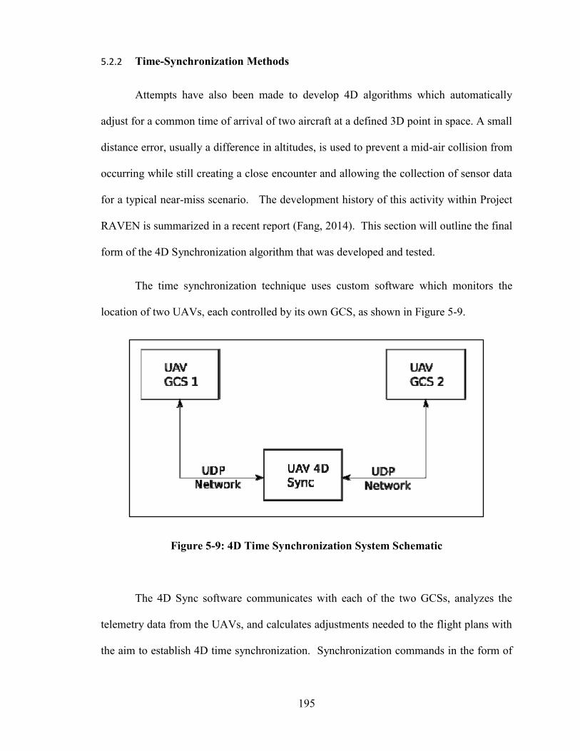
195
5.2.2 Time-Synchronization Methods
Attempts have also been made to develop 4D algorithms which automatically
adjust for a common time of arrival of two aircraft at a defined 3D point in space. A small
distance error, usually a difference in altitudes, is used to prevent a mid-air collision from
occurring while still creating a close encounter and allowing the collection of sensor data
for a typical near-miss scenario. The development history of this activity within Project
RAVEN is summarized in a recent report (Fang, 2014). This section will outline the final
form of the 4D Synchronization algorithm that was developed and tested.
The time synchronization technique uses custom software which monitors the
location of two UAVs, each controlled by its own GCS, as shown in Figure 5-9.
Figure 5-9: 4D Time Synchronization System Schematic
The 4D Sync software communicates with each of the two GCSs, analyzes the
telemetry data from the UAVs, and calculates adjustments needed to the flight plans with
the aim to establish 4D time synchronization. Synchronization commands in the form of
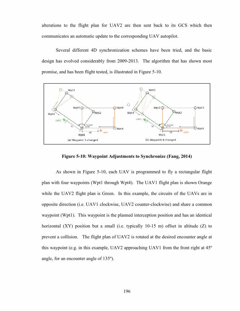
196
alterations to the flight plan for UAV2 are then sent back to its GCS which then
communicates an automatic update to the corresponding UAV autopilot.
Several different 4D synchronization schemes have been tried, and the basic
design has evolved considerably from 2009-2013. The algorithm that has shown most
promise, and has been flight tested, is illustrated in Figure 5-10.
Figure 5-10: Waypoint Adjustments to Synchronize (Fang, 2014)
As shown in Figure 5-10, each UAV is programmed to fly a rectangular flight
plan with four waypoints (Wpt1 through Wpt4). The UAV1 flight plan is shown Orange
while the UAV2 flight plan is Green. In this example, the circuits of the UAVs are in
opposite direction (i.e. UAV1 clockwise, UAV2 counter-clockwise) and share a common
waypoint (Wpt1). This waypoint is the planned interception position and has an identical
horizontal (XY) position but a small (i.e. typically 10-15 m) offset in altitude (Z) to
prevent a collision. The flight plan of UAV2 is rotated at the desired encounter angle at
this waypoint (e.g. in this example, UAV2 approaching UAV1 from the front right at 45º
angle, for an encounter angle of 135º).
197
The 4D synchronization algorithm leaves the UAV1 flight plan unchanged, and
makes automatic adjustments to the UAV2 flight plan in real time. The goal is to
minimize the distance error (d1-d2) as the two aircraft are both approaching Wpt1. When
this distance error is tuned to zero, 4D synchronization is achieved. The algorithm first
adjusts the airspeed of UAV2 in an attempt to synchronize to a common time of arrival at
Wpt1. However, the range of safe airspeed adjustments and the rate by which they will
have the desired effect on the UAV is limited, especially when real-world flight
conditions (winds) are considered. Once these limits are reached, the algorithm then uses
adjustments to the UAV2 flight plan, by making adjustments to the location of Wpt3 as
shown in Figure 5-10 (a). Moving Wpt3 inwards (toward the lower right) will decrease
the time needed for UAV2 to reach Wpt1, and moving it outwards will increase the time.
The algorithm uses these adjustments to Wpt3 until the limit to what is possible is reached
(i.e. when the error d1-d2 cannot be decreased any further). Adjustments to Wpt4 are
then used in a similar manner to fine-tune the 4D synchronization as shown in the Figure
5-10 (b).
The success of the algorithm, and the speed at which it converges to a 4D
synchronization solution depends strongly on the flight conditions (i.e. especially the
presence or absence of strong or variable winds) and the starting situation of the two
UAVs. The algorithm assumes that the UAVs have already been roughly synchronized
using course methods by the GCSs, and are flying under autopilot control such that the
UAVs are each on the final “legs” (Wpt4 to Wp1) of their flight plan when the 4D
synchronization algorithm is engaged. An average of three or four circuits are typically
needed before 4D synchronization is achieved (Fang, 2014).

198
This time-synchronization method has been used with some success during
practical field trials at Argentia, including tests conducted in late September 2013.
During these trials this author was the manual pilot for one of the two UAVs involved.
As observed during these tests, provided the aircraft are flown with properly-tuned
autopilots and in reasonable wind conditions, head-on, chasing and 135º encounter
scenarios similar to the example shown in this section can be achieved. However, the
difficulties in maintaining constant altitudes and accurate airspeeds have hampered
attempts to record a good set of video footage for such scenarios. Given the field of view
of most cameras, the size of the aircraft involved and their relative speeds, even if an
interception is missed by only a few seconds, the encounter footage (if any) will be
limited.
The 4D Sync method described here does show promise but clearly more work is
needed to provide a truly autonomous method of achieving 4D synchronization and
permitting the collection of a rich set of 4D encounter data.
5.2.3 The PHI Maneuver
During simulated testing of opposing circuits within the 4D Simulation
Environment, a new method was discovered. While setting up opposing circuits, one of
the aircraft was forced to intercept a waypoint that was inside its minimum turn radius.
Most autopilots like the Piccolo II feature an escape algorithm to prevent this situation, by
forcing the UAV to fly to the next waypoint if it is impossible for it to reach the current
one in a certain time limit. However, the representation used in the 4D Simulation does
not have this algorithm. Instead, the aircraft continued to turn in an attempt to intercept
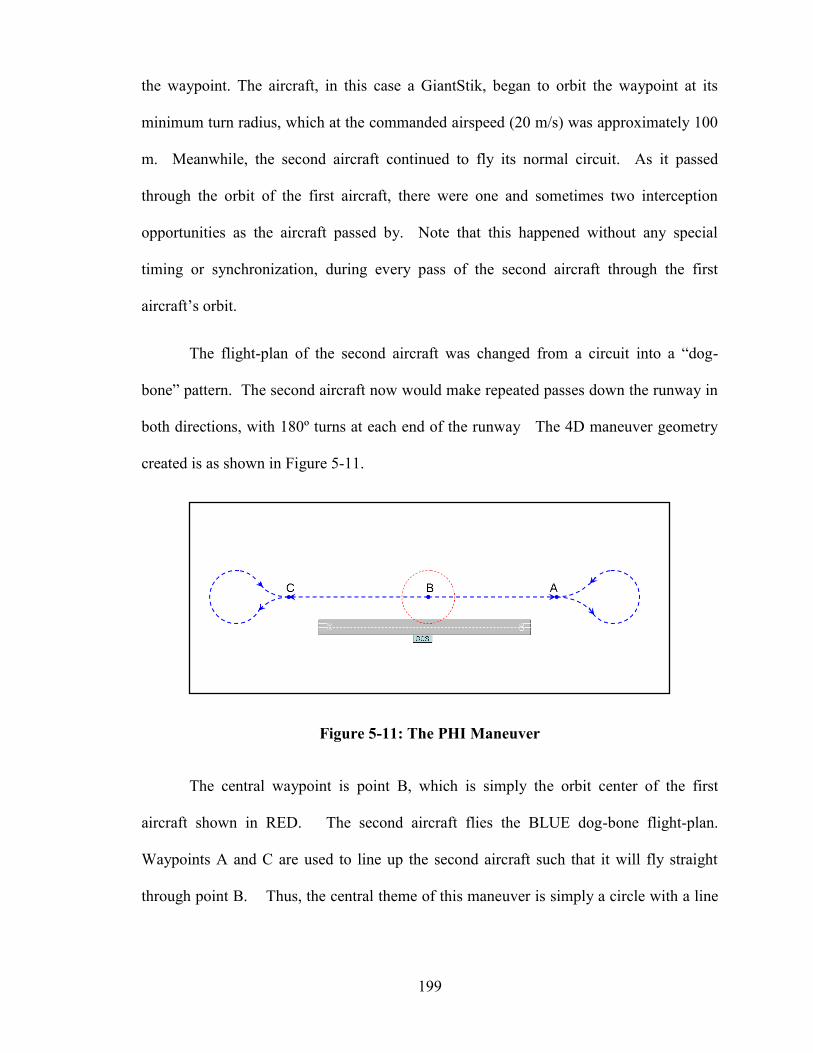
199
the waypoint. The aircraft, in this case a GiantStik, began to orbit the waypoint at its
minimum turn radius, which at the commanded airspeed (20 m/s) was approximately 100
m. Meanwhile, the second aircraft continued to fly its normal circuit. As it passed
through the orbit of the first aircraft, there were one and sometimes two interception
opportunities as the aircraft passed by. Note that this happened without any special
timing or synchronization, during every pass of the second aircraft through the first
aircraft’s orbit.
The flight-plan of the second aircraft was changed from a circuit into a “dog-
bone” pattern. The second aircraft now would make repeated passes down the runway in
both directions, with 180º turns at each end of the runway The 4D maneuver geometry
created is as shown in Figure 5-11.
Figure 5-11: The PHI Maneuver
The central waypoint is point B, which is simply the orbit center of the first
aircraft shown in RED. The second aircraft flies the BLUE dog-bone flight-plan.
Waypoints A and C are used to line up the second aircraft such that it will fly straight
through point B. Thus, the central theme of this maneuver is simply a circle with a line
200
through it – resembling the Greek letter Ф (PHI). It is from this resemblance that the
name “PHI Maneuver” has been created. The simplicity of this maneuver is that only one
waypoint needs to be defined accurately. As shown this should be shifted away from the
GCS so that the encounter area is always in front. Most commercial autopilots have a
waypoint-orbit capability built-in so the RED flight-plan is easy to define. The radius
should be chosen such that it is a wider than the minimum turn radius of the aircraft.
Otherwise, the orbital radius will effectively become this minimum radius. The AP will
struggle to maintain the aircraft in a stable orbit that is on the edge of what the vehicle can
do aerodynamically. By leaving some margin for an inward turn, the maneuver options
for the orbiting aircraft are also kept open.
The other aircraft only has to fly through waypoint B to guarantee at least one 4D
encounter for every pass. The random nature of the 4D encounters created by this
maneuver geometry will be such that the exact locations of each aircraft will not be
known ahead of time. The range of each encounter will also be random. This assumes no
enhancements are used to improve the chances of an interception.
5.2.4 The PHI Maneuver with Active Guidance
The 4D Simulation has been used to experiment with the concept of giving one of
the aircraft active interception guidance control, similar to that of an air-to-air missile, to
force an encounter. Note that only a high level discussion of these experiments is given
here. Detailed simulation results are provided in Section 5.4.
The orbiting aircraft was given a simple interception guidance program, which
remains dormant while the second aircraft is far away. Once the second aircraft comes

201
within range of the orbiting aircraft, it goes from being “passive” to “active”, and
attempts to intercept the approaching aircraft. Simple Pursuit was used initially, where
the heading command has set equal to the instantaneous bearing to target. However, as
expected this almost always resulted in the pursuing aircraft flying behind and chasing the
second aircraft, especially if the aircraft was being forced to exceed its maximum turn
rate. The difference in airspeeds was usually not enough to give the interceptor any
advantage once it was chasing the target, so the interception never happened. The target
aircraft simply flew away, beyond the active pursuit range, and the interception attempt
was stopped. The orbiting aircraft then returned to its previous (orbit) program to wait for
the next opportunity.
It was when the GNC method was switched to Proportional Navigation (PN)16
that
the results got more interesting. Unlike Simple Pursuit, PN adjusts the course of the
intercepting aircraft such that the bearing angle to the target remains fixed. This
adjustment occurs automatically even if either aircraft are actively maneuvering, and
usually results in the interceptor “leading the target”, a very common technique used by
dog-fighting pilots using machine guns. Simple Pursuit was abandoned decades ago as a
missile GNC method and replaced by PN, precisely for the reasons encountered in the last
paragraph (Abramovitz, 1953). PN is also one of the few GNC strategies that can allow
an interception when there is a large difference between target and interceptor velocities
(Stallard, 1968).
16 A detailed description of the Proportional Navigation Guidance method is provided in Section 5.3.3.2.
202
Using PN, the orbiting aircraft was able to intercept the approaching target aircraft
with fair regularity, once the PN gain and maximum bank angle of the interceptor were
properly adjusted. In several cases, a side-ways encounter was quickly followed by a
second pursuit-style tail-on encounter. The chance of a successful encounter appeared to
be associated with where the aircraft was in its orbit when the approaching aircraft was
first detected. The best situations were when the interceptor was turning past the 12 or 6
o’clock positions relative to the runway direction, and with the aircraft approaching in
front of the interceptor.
An alternative strategy is to provide the aircraft flying the “dog-bone” pattern with
the interception GNC program, while the target assumes the orbit pattern. This resulted
in even more dramatic interceptions, especially when the intruder aircraft was given a
detection range of between two and three times the orbital radius of the loitering aircraft.
The intruder aircraft was able to intercept the loitering aircraft once per pass and once
again attempted multiple interceptions.
5.3 Avoidance Maneuvers
In this section we will discuss avoidance maneuvers. Assuming one aircraft has
detected a collision threat posed by another aircraft, what should it do next? Is an
avoidance maneuver possible or safe? If an avoidance maneuver is performed, what is
the most effective (and safe) method?
5.3.1 Rules of the Air and Right-of-Way
Before any avoidance maneuver strategy can be proposed, it is important to
consider what rules or regulations apply. The following discussion will make reference

203
to the Canadian Aviation Regulations (CARs). A summary of the regulations applicable
to this subject material is also provided in Appendix C. Here we will concentrate on the
rules which apply to the collision avoidance problem. Assuming the manned aircraft pilot
is obeying these rules, it may be assumed that he/she will attempt to follow them while
attempting to avoid collisions. The small UAV should try to follow these same rules in
order to be a predictable and cooperative member of the air traffic.
It is the responsibility of every pilot-in-command to be aware of his surroundings
(FAA AC-90-48-C, 1983), follow ATC directions, and obey the Rules of the Air in such a
way as to minimize the risk of traffic conflicts. For example, by following the cruising
altitude rules for VFR and IFR traffic, this should in theory guarantee at least 500 ft
vertical separation by opposing traffic17
. Note that this does not prevent the situation of
two aircraft which might be on converging courses both at the same altitude, when both
are headed in more or less the same direction.
The manned pilot is also responsible to remain “well clear” of other aircraft and to
stay clear of clouds when flying by VFR. In this thesis a spherical distance of 500 ft has
been assumed. However is must be pointed out that this is not rigorously defined in
manned aviation regulations. The 500 ft value represents the notion of safe minimum
separation as commonly used by GA pilots. This differs from the “well clear” notion as
held by commercial pilots and military pilots who are more accustomed to ATC
definitions of horizontal separation minima which are usually quoted as a minimum time
separation between high-speed aircraft. The lack of agreement on what is a quantitative
17 A summary of applicable Canadian Aviation Regulations (CARs) related to cruising altitudes is provided in Appendix C.
204
and rigorous definition of “well clear” has been the subject of a great deal of discussion
amongst UAV researchers. The lack of a quantitative definition was identified very
recently by an FAA Workshop as a major research requirement to allow development of
effective DSA capabilities to proceed (FAA Sense and Avoid Workshop, 2013). There
has been very recent consensus reached that the “well clear” definition developed at MIT
Lincoln Labs may be the ideal candidate in terms of compatibility with existing manned
aviation including TCAS. This candidate “well clear” definition is a cylindrical zone
center on the UAV with a radius of 4000 ft and height of 700 ft (Cook, Brooks, Cole,
Hackenberg, & Raska, 2014).
There are minimum altitudes that must also be followed. In Canada, these are
1000 ft above the highest obstacle while in cruise and 500 ft minimum altitude in remote
uncontrolled airspace, and at least 1000 ft minimum above any built-up area (MacDonald
& Peppler, pp. 114-117). Implied in the regulations is the assumption that the pilot
provides a last-ditch capability if these rules fail to maintain good separation, especially
with other aircraft (FAA AC-90-48-C, 1983).
The Right-of-Way rules also specify the correct course of action in the case of a
potential traffic conflict. Right-of-Way must be yielded to the air vehicle of lesser
maneuverability, i.e. first balloons, then airships (rare but still in the regulations), gliders,
and finally powered aircraft. UAVs are generally considered as having lower priority
versus equivalent powered (manned) aircraft, and must yield to manned aircraft. This last
rule is not in the CARs, but has been the effective operating practice by TC Canada when
granting UAV operators SFOCs.
205
If two aircraft find themselves on a head-on collision course, the rule is to always
turn right. If an aircraft is approaching from behind and overtaking another aircraft, it
should bear right and pass well to the right (at least 500 ft horizontal minimum distance)
of the other aircraft. If two aircraft are on converging courses, the aircraft on the right
has the Right-of-Way and should maintain its course and speed. The aircraft on the left is
required to alter his course to avoid the collision. However, the rules still state the aircraft
on the right must still maintain vigilance and take whatever actions are necessary to avoid
a collision (MacDonald & Peppler, p. 108)
The Right-of-Way rules also state that, in general, the aircraft required to give way
should never maneuver in such a way such that it passes over, under or crosses in front of
the other aircraft. This last rule is important when considering how UAV collision
avoidance maneuvers should be handled.
5.3.2 Manned Aircraft versus UAVs
It is a misconception when people speak of UAVs colliding with manned aircraft,
especially when the small UAV is considered. The implication is that the UAV strikes
the manned aircraft, akin to an interception by a missile, with no fault due to the manned
aircraft motion A similar misconception is frequently encountered during discussions of
collisions between aircraft and birds, the so-called “bird strike”. Perhaps the most
dramatic recent event was the “miracle on the Hudson” incident in 2009, when an Airbus
A320 flew through a flock of Canada Geese shortly after takeoff from La Guardia airport
in New York City. This resulted in multiple bird-strikes including several being sucked
into both engines – and the rare but dreaded dual-engine failure. This forced the pilot
206
crew to accomplish one of the few successful water landings “ditches” by an airliner
(NTSB/AAR-10/03, 2010). Note that while climbing after takeoff like this A320 was,
airliners are accelerating to about 250 kts while below 10,000 ft. Meanwhile Geese fly at
between 30-40 MPH (26-35 kts) (Hoar, De Smet, Campbell, & Kennedy, 2010). The
airliner outclasses the birds in speed by almost an order of magnitude (i.e. almost ten
times). Any attempt by the birds to “dodge” such an on-coming aircraft is clearly futile.
A similar situation applies to the small UAV. A small UAV like the Aerosonde
cruises at 55-60 kts. Manned aircraft will typically outclass the small UAV speed by at
least two to three times. For example, GA aircraft such as a Cessna C172 cruises at 125
kts (i.e. about twice the top speed of an Aerosonde) while a Beechcraft King Air cruises
at 289 kts (i.e. almost five times faster). In Chapter 4 we have estimated the theoretical
minimum sighting distances and the probability that a human would spot a small UAV.
Even under ideal conditions, most human pilots are unlikely to spot an Aerosonde until a
range of under 500m. This leaves mere seconds for the human pilot to spot the UAV,
recognize the danger and start a maneuver. As with the situation with the birds, it is more
likely that the manned aircraft will be completely oblivious to the presence of the
Aerosonde and will fly straight through it.
Therefore, short of the UAV using visual enhancement methods or a transponder
to alert manned aircraft at long range, we must assume that the onus will be on the UAV
to detect the on-coming aircraft, and attempt an avoidance maneuver. The chance of
success will depend greatly on how soon the UAV is able to detect the approaching
aircraft, and the relative velocities involved.

207
5.3.2.1 Horizontal Avoidance Maneuvers
In this initial analysis we will ignore altitude and assume the two aircraft are
roughly at the same altitude such that the situation is essentially 2D. Consider the
diagram in Figure 5-12, which shows a hypothetic situation of a UAV flying North (top
of the page) as shown. We next assume threat aircraft approaching the UAV from three
directions, head-on (A), side-ways (B) and back-on (C). If we impose a requirement to
maneuver out of the path of the on-coming aircraft such that at least 500 ft (150 m)
separation is achieved, we may now estimate the limits of what the UAV can do in each
situation.
The head-on (A) is the worst case, as the closure velocity will be the sum of the
threat aircraft and UAV speeds (i.e. Va/c + VUAV). The UAV must attempt to turn right
and exit the 500 ft (150 m) threat area as quickly as possible. Assuming a minimum turn
radius of 150 m, which is typical for an Aerosonde flying at 58 kts (~30 m/s), it will take
the curved path as shown in green, or about one quarter the circumference of a 150 m
radius circle. This will take about 7.8 seconds to accomplish. The futility of the manned
aircraft attempting to maneuver with only a few seconds left at 500 m now becomes clear.
For the side-ways case (B), the closure velocity to the current center position of
the 500’ threat circle is simply the velocity of the threat aircraft (i.e. Va/c). In this
situation, the UAV should simply fly straight ahead, as this is the fastest way (5 sec) to
clear the 150m radius circle. This is an example where maintaining the current course
and speed is the best strategy for the UAV.
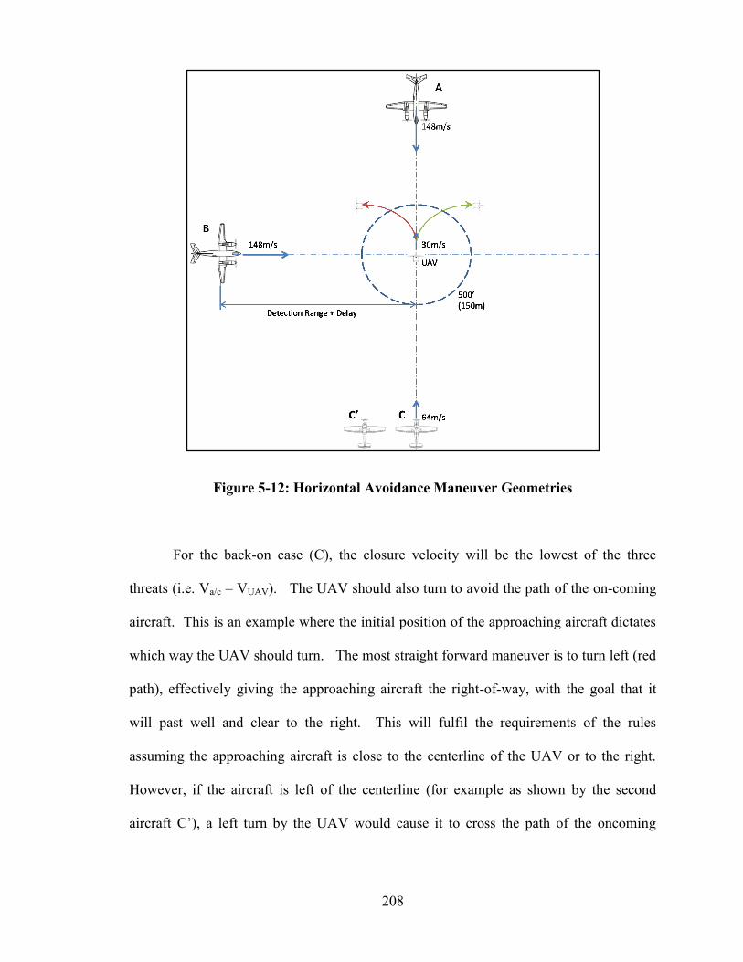
208
Figure 5-12: Horizontal Avoidance Maneuver Geometries
For the back-on case (C), the closure velocity will be the lowest of the three
threats (i.e. Va/c – VUAV). The UAV should also turn to avoid the path of the on-coming
aircraft. This is an example where the initial position of the approaching aircraft dictates
which way the UAV should turn. The most straight forward maneuver is to turn left (red
path), effectively giving the approaching aircraft the right-of-way, with the goal that it
will past well and clear to the right. This will fulfil the requirements of the rules
assuming the approaching aircraft is close to the centerline of the UAV or to the right.
However, if the aircraft is left of the centerline (for example as shown by the second
aircraft C’), a left turn by the UAV would cause it to cross the path of the oncoming
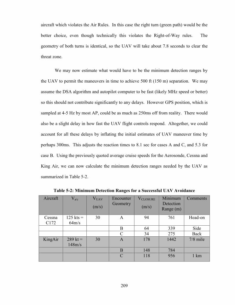
209
aircraft which violates the Air Rules. In this case the right turn (green path) would be the
better choice, even though technically this violates the Right-of-Way rules. The
geometry of both turns is identical, so the UAV will take about 7.8 seconds to clear the
threat zone.
We may now estimate what would have to be the minimum detection ranges by
the UAV to permit the maneuvers in time to achieve 500 ft (150 m) separation. We may
assume the DSA algorithm and autopilot computer to be fast (likely MHz speed or better)
so this should not contribute significantly to any delays. However GPS position, which is
sampled at 4-5 Hz by most AP, could be as much as 250ms off from reality. There would
also be a slight delay in how fast the UAV flight controls respond. Altogether, we could
account for all these delays by inflating the initial estimates of UAV maneuver time by
perhaps 300ms. This adjusts the reaction times to 8.1 sec for cases A and C, and 5.3 for
case B. Using the previously quoted average cruise speeds for the Aerosonde, Cessna and
King Air, we can now calculate the minimum detection ranges needed by the UAV as
summarized in Table 5-2.
Table 5-2: Minimum Detection Ranges for a Successful UAV Avoidance
Aircraft Va/c VUAV
(m/s)
Encounter
Geometry
VCLOSURE
(m/s)
Minimum
Detection
Range (m)
Comments
Cessna
C172
125 kts =
64m/s
30 A 94 761 Head-on
B 64 339 Side
C 34 275 Back
KingAir 289 kt =
148m/s
30 A 178 1442 7/8 mile
B 148 784
C 118 956 1 km

210
Although the situation is not quite as bad as for the Canada Geese, it is clear that
the detection requirements for the UAV are demanding. In the case of the Cessna threat,
the UAV would require detection at 761 m or more to ensure enough time to avoid it by
500 ft (150 m) in the worst case head-on scenario. For the faster King Air threat, the
required detection range is 1442 m or about 7/8 of a statute mile. It will be very difficult
to equip the small UAV with sensors capability of reliably detecting aircraft at these
ranges, although a detection range of 500 m or 1000 m may be possible using existing
EO/IR methods (Kharhoff, Limb, Oravsky, & Shephard, 2006).
5.3.2.2 Vertical Avoidance Maneuvers
The previous section assumed only a 2D approach to the avoidance strategy,
which forces the UAV detection system to have a range capability of 761 m assuming a
GA aircraft head-on collision threat. However, the UAV may be able to improve the
chances of avoiding a collision by using vertical maneuvers. While such an avoidance
maneuver would be undesirable on a manned aircraft for obvious safety reasons, the
unmanned UAV could perform a sudden “crash dive” towards the ground. This would
take advantage of the natural assistance of gravity, and is a common technique used by
birds to avoid predators (Hoar, De Smet, Campbell, & Kennedy, 2010).
Given the limited time available to accomplish a separation maneuver, it can be
shown that the dive maneuver is the quickest method available. The UAV of course must
have sufficient altitude to accomplish a drop of 500 ft (150 m) while still maintaining
sufficient altitude above the ground. If we are strict about the minimum altitude rule (500
ft AGL) this implies such a dive maneuver would only be appropriate at altitudes of at

211
least 1000 ft AGL. However, in the interests of flight safety the UAV might be allowed
to dive to very low altitudes (i.e. 100-200 ft AGL) in remote un-inhabited areas - much
lower then what would be considered safe for manned aircraft. Thus, the dive might be
done at as low as 600-700 ft AGL altitude.
Assuming the goal of a drop of 500 ft, we can estimate how fast the UAV can
accomplish this feat. If we assume the UAV is able to dive by a very steep angle, say 60º
while maintaining the same forward speed, and pull out at the bottom of the dive, the
maneuver then becomes a vertical “S-curve” as shown in Figure 5-13.
Assuming the UAV can maintain its normal airspeed, once the dive angle is
established the effective vertical component of its velocity would start at about 26 m/s but
would accelerate due to gravity (i.e. 9.8 m/s2). From simple kinematics, we can calculate
the time required to accomplish the 150 m drop as follows:
Figure 5-13: Vertical Avoidance Maneuver for UAVs
212
𝑆𝑦 = 𝑉𝑦𝑡 +1
2𝐴𝑦𝑡2 (5-18)
150 𝑚 = (26 𝑚/𝑠)𝑡 +1
2(9.8 𝑚/𝑠2)𝑡2
∴ 𝑡 = 3.48𝑠
Therefore this maneuver can be accomplished in about 3.5 seconds, for an
effective descent rate of 42.8 m/s, which is over 8000 feet per minute.18
The equivalent detection ranges needed by the UAV to accomplish this vertical
avoidance maneuver may now be estimated. Assuming similar GPS and control delays as
before, approximately 3.8 sec is needed. We can now consider just the approaching
aircraft velocity (equivalent to the horizontal B case), and from this find that the detection
range required is 243 m for the Cessna, and 562 m for the King Air. If the dive was
combined with heading change (i.e. to prevent over-flight for the head-on or tail-on cases)
this would be a very effective avoidance method. The foregoing discussion assumes the
UAV airframe is capable of sustaining the high accelerations implied without suffering
structural failure, especially of the main wing or control surfaces. However, even if a
more modest dive angle of 45º is used and the above analysis repeated, it is found that the
detection ranges needed are reasonable, approximately 262 m in the case of a Cessna, and
606 m for the King Air.
18 This estimate assumes the AP allows the acceleration due to gravity to occur, which is the normal case when the AP responds to a sudden step change in the commanded altitude. If it actively controls the descent (i.e. maintaining airspeed) the dive can still be
accomplished in about 5.7 seconds.

213
5.3.2.3 The Danger of Last-Minute Avoidance Maneuvers
It is important to realize that an incorrect avoidance maneuver may be counter-
productive and could in fact increase the risk of a collision. This includes incorrectly
deciding which way to turn, as discussed in the horizontal avoidance case for scenario C
in the previous section. Care must always be taken to make sure the avoidance maneuver
causes an increase in the separation range and prevents over-flights, under-flights or
crossing the path of the other aircraft. Even in the straight forward case of the head-on
situation, where both aircraft turn right, the evasion maneuvers must be initiated at
sufficient range to prevent the cross-path situation.
The chance of a collision is also increased dramatically due to the fact that aircraft
turns usually involve a bank angle. If we consider two aircraft on a head-on (or tail-on)
collision course, there is actually a relatively small cross-sectional area where a collision
can occur, assuming neither aircraft turns. This is easier to explain by reference to the
diagram of Figure 5-14 (Hobbs, p. 22) which shows the threat area for two high-wing
aircraft of roughly the same size. If the wings are keep level as in the top case, there is a
relatively small intersection area. However, if the aircraft were to bank as shown in the
bottom case, the intersection area increases dramatically due to the interaction between
the wings. If we consider the risk of collision to be proportional to these intersection
areas, the chance of a collision has increased by as much as four times.
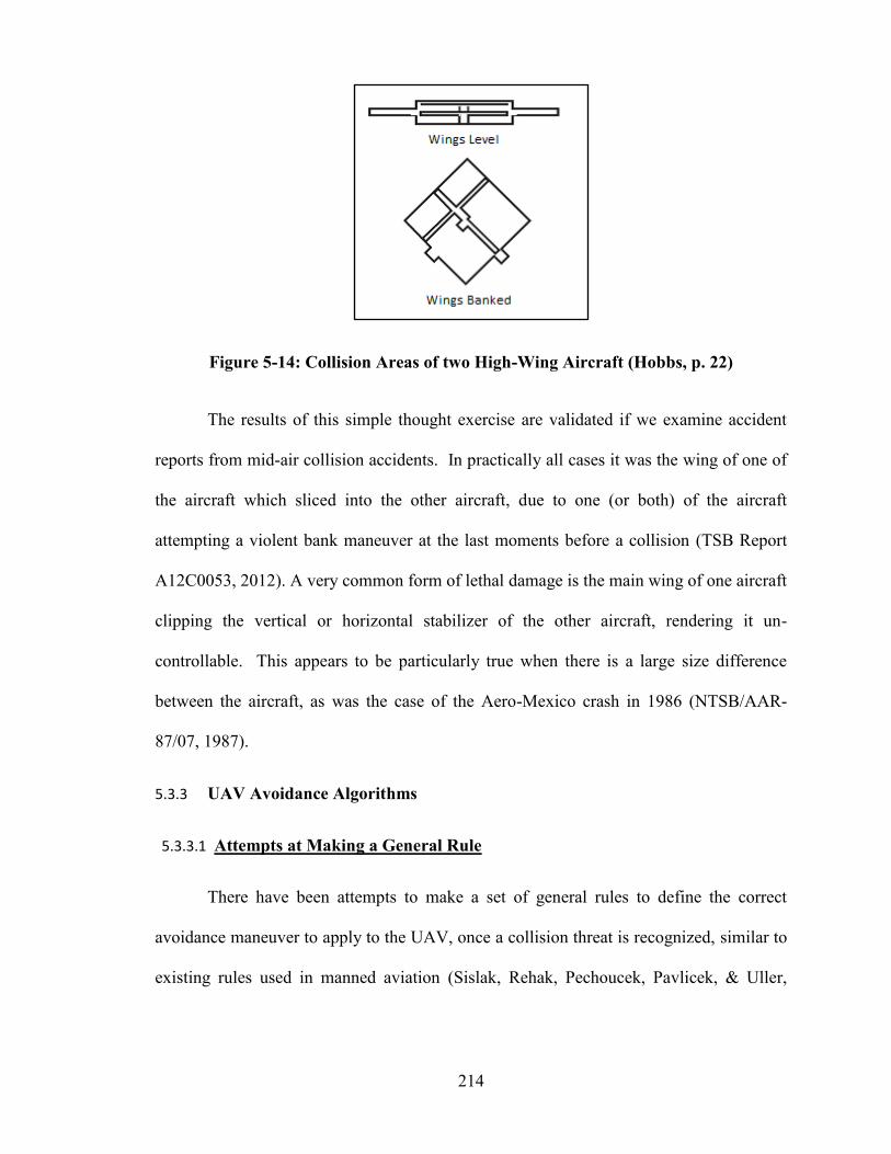
214
Figure 5-14: Collision Areas of two High-Wing Aircraft (Hobbs, p. 22)
The results of this simple thought exercise are validated if we examine accident
reports from mid-air collision accidents. In practically all cases it was the wing of one of
the aircraft which sliced into the other aircraft, due to one (or both) of the aircraft
attempting a violent bank maneuver at the last moments before a collision (TSB Report
A12C0053, 2012). A very common form of lethal damage is the main wing of one aircraft
clipping the vertical or horizontal stabilizer of the other aircraft, rendering it un-
controllable. This appears to be particularly true when there is a large size difference
between the aircraft, as was the case of the Aero-Mexico crash in 1986 (NTSB/AAR-
87/07, 1987).
5.3.3 UAV Avoidance Algorithms
5.3.3.1 Attempts at Making a General Rule
There have been attempts to make a set of general rules to define the correct
avoidance maneuver to apply to the UAV, once a collision threat is recognized, similar to
existing rules used in manned aviation (Sislak, Rehak, Pechoucek, Pavlicek, & Uller,

215
2006). Examples are the rule to always right in the case of a head-on encounter, and to
bear left for the tail-on case, such that approaching aircraft will pass to the right.
However, even for these simple encounter geometries, depending on the relative positions
and velocities of the two aircraft, there will always be exceptions where rule-based
maneuvers might actually decrease safety.
Figure 5-15: Different Head-On Encounter Trajectories
To illustrate, consider the situation shown in Figure 5-15, which shows three
different head-on encounters of an aircraft and an UAV, but with slightly different off-
axis velocities as shown. In each case, the future (unmodified) course is projected,
representing the situation where the manned aircraft has not detected the UAV. For
Aircraft A, the right turn strategy by the UAV (green path) makes sense and results in a
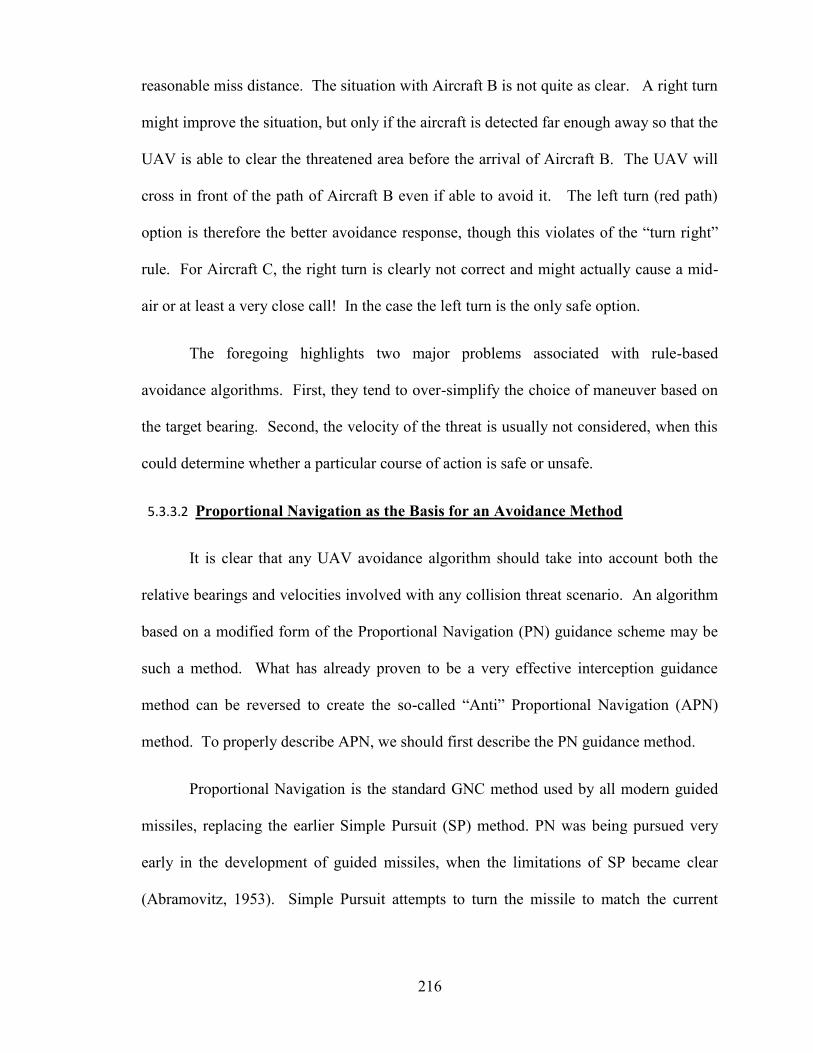
216
reasonable miss distance. The situation with Aircraft B is not quite as clear. A right turn
might improve the situation, but only if the aircraft is detected far enough away so that the
UAV is able to clear the threatened area before the arrival of Aircraft B. The UAV will
cross in front of the path of Aircraft B even if able to avoid it. The left turn (red path)
option is therefore the better avoidance response, though this violates of the “turn right”
rule. For Aircraft C, the right turn is clearly not correct and might actually cause a mid-
air or at least a very close call! In the case the left turn is the only safe option.
The foregoing highlights two major problems associated with rule-based
avoidance algorithms. First, they tend to over-simplify the choice of maneuver based on
the target bearing. Second, the velocity of the threat is usually not considered, when this
could determine whether a particular course of action is safe or unsafe.
5.3.3.2 Proportional Navigation as the Basis for an Avoidance Method
It is clear that any UAV avoidance algorithm should take into account both the
relative bearings and velocities involved with any collision threat scenario. An algorithm
based on a modified form of the Proportional Navigation (PN) guidance scheme may be
such a method. What has already proven to be a very effective interception guidance
method can be reversed to create the so-called “Anti” Proportional Navigation (APN)
method. To properly describe APN, we should first describe the PN guidance method.
Proportional Navigation is the standard GNC method used by all modern guided
missiles, replacing the earlier Simple Pursuit (SP) method. PN was being pursued very
early in the development of guided missiles, when the limitations of SP became clear
(Abramovitz, 1953). Simple Pursuit attempts to turn the missile to match the current
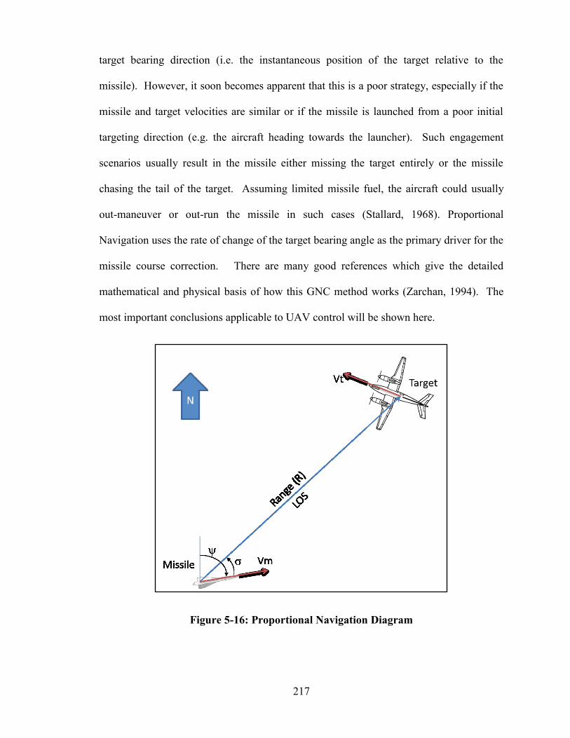
217
target bearing direction (i.e. the instantaneous position of the target relative to the
missile). However, it soon becomes apparent that this is a poor strategy, especially if the
missile and target velocities are similar or if the missile is launched from a poor initial
targeting direction (e.g. the aircraft heading towards the launcher). Such engagement
scenarios usually result in the missile either missing the target entirely or the missile
chasing the tail of the target. Assuming limited missile fuel, the aircraft could usually
out-maneuver or out-run the missile in such cases (Stallard, 1968). Proportional
Navigation uses the rate of change of the target bearing angle as the primary driver for the
missile course correction. There are many good references which give the detailed
mathematical and physical basis of how this GNC method works (Zarchan, 1994). The
most important conclusions applicable to UAV control will be shown here.
Figure 5-16: Proportional Navigation Diagram

218
Consider the proportional navigation situation as illustrated in Figure 5-16. The
missile is assumed to have a seeker in the nose which is able to track the location of the
target. At the moment depicted, the missile and target are both moving at different
velocities and headings. Relative to the missile, the target will be located at a Range (R),
and at a Line-of-Sight (LOS) angle (σ). Due to the relative motions of both objects, this
angle will likely be changing (�̇�) as shown. It may be shown that the missile should
adjust its heading to counter this angle change according to the law:
ѱ̇ = 𝐾 ∗ 𝜎 ̇ (5-19)
Where,
K = Proportional Navigation constant (Gain)
�̇� = rate of change of the LOS angle
ѱ̇ = rate of change of missile heading
This GNC law will have the effect to null-out the LOS rate until it becomes zero
(i.e. �̇� = 0). The choice of K depends on how aggressive a maneuver is required or
desired, and the turn-rate capabilities of the missile. A value of 3-5 is typical, but 10 may
be needed to accommodate head-on engagements (Stallard, 1968). This navigation
method will automatically adjust to any LOS changes caused by either the target or the
missile. Assuming a constantly decreasing range, this will eventually set up the situation
of a fixed target bearing, with the missile “leading the target” to a common
intercept/impact point as illustrated in Figure 5-17.
219
Figure 5-17: Constant-Bearing Leading to a Collision
This is the same principal known for centuries in nautical navigation as the
Constant Bearing Decreasing Range situation (O'Brian, 1996). If the relative bearing
angle between your vessel and another vessel is constant, and assuming the range is
decreasing, you will eventually collide with the other vessel. Sailors are taught to avoid
this hazardous situation by turning in such a way to change the bearing angle to the other
ship. Ideally, this should also be done with the aim to increase the range between them.
This forms an excellent basis for an avoidance algorithm for UAVs.

220
5.3.3.3 Anti-Proportional Navigation as an Avoidance Algorithm
The PN algorithm was first applied in the 4D DSA simulation to give the Intruder
aircraft interception guidance. While setting up this PN scheme, a sign error was made
in the LOS angle correction which had the effect of creating a course correction away
from the Target, resulting in the Intruder engaging in an evasive maneuver. For example,
if the LOS angle was decreasing to zero in a counter-clockwise direction, the aircraft
would suddenly turn right of the target and miss it entirely. Likewise, if the LOS was
decreasing in a clockwise direction, the intruder course veered to the left. Since the
desired behaviour was to intercept, the sign error was fixed – but this was another
example of an accidental discovery during this research, and hinted at a very promising
avoidance method.
A literature search was conducted and confirmed that the erroneous PN algorithm
initially programmed was in fact a form of the Anti-Proportional Navigation scheme as
investigated by others (Ham & Bang, 2004). It is noted by several authors that even a
modest APN gain of 3 appears to be sufficient to create an effective avoidance maneuvers
for typical small UAVs, provided the other aircraft is detected at sufficient range (George
& Ghose, 2009). A detection range of 300-500 m appears to be the minimum needed to
guarantee a 500 ft miss distance. The simplest way to implement the APN is to use the
same guidance law suggested by equation 5-19 but with a negative value for the gain (K).
The APN avoidance GNC algorithm has been implemented in the 4D Simulation.
Preliminary results indicate this is a very effective avoidance method, and takes care of
the 2-D azimuth avoidance direction automatically. It is also possible to implement APN

221
in the vertical direction too, but a simpler approach is to combine the APN maneuver in
the horizontal plane with a simple vertical dive maneuver.
5.4 Predicted 4D Simulation Results
This section presents simulation results of the more promising 4D encounter and
avoidance strategies covered previously in this chapter. The 4D simulation was setup
using the PHI maneuver as described in Section 5.2.3, using the Clarenville Airstrip as the
test site. Both aircraft were configured to be GiantStik aircraft, and thus of the same
aerodynamic capability. In the following results the Intruder was programmed to fly the
dog-bone waypoint flight plan. The Target was programmed to orbit a waypoint at the
mid-point of the runway at a radius of 200 m.
5.4.1 Base PHI-Maneuvre Results (Passive Aircraft)
In these tests, the aircraft were allowed to fly their autopilot programs in a passive
mode (i.e. neither using any form of active guidance). The simulation was run for one
hour (3600 sec). An encounter was considered to start once the range between the
vehicles was 300 m or less, and ended once the range was over 300 m. During each
encounter, both instances of the 4D simulation calculated and recorded the instantaneous
range and bearing to the other aircraft. These results were post-processed to yield the
polar plots presented below. Figure 5-18 shows these results from the point of view of
the Target aircraft. In the left image, the trajectory of each encounter is shown as a black
line. The point of closest approach for each encounter is circled in red. For clarity, the
right image has the trajectories removed.

222
Figure 5-18: Encounters during Passive PHI Maneuvers; (left) Trajectories and
Closest Approaches; and (right) Closest Approaches.
There were at total of 40 encounters during the scenario (i.e. for a rate of 40/hour).
This agrees with a theoretical estimate of one encounter every 90 seconds based solely on
the geometry of the dog-bone waypoint pattern used by the Intruder. The Intruder passes
by the Target at a variety of ranges up to a maximum of 200 m. There were several
passes when the Intruder essentially intercepted the Target (i.e. < 3 m range). The
relative bearings of the closest approaches are distributed around the Target, with the
furthest approaches being biased along the 155 - 335º cardinal directions, which is at a
right angle to the runway heading.
5.4.2 Active Interceptions by the Intruder (Target Passive)
The Intruder aircraft was given active interception guidance using Proportional
Navigation (PN). A PN constant (K) between three and five was tried. The results shown

223
here are for the K=5 case. The Intruder would now attempt an interception as soon as the
range to the Target dropped below the detection range of 300 m. The Target was left
passive and programmed to continue its orbit program without any reaction. To limit the
number of encounters to a single attempt per pass, the PN algorithm was programmed to
break off the intercept attempt when the range to the Target began to increase. This
scenario was run for 3600 sec, which resulted in the encounters as shown in Figure 5-19.
Figure 5-19: Active Intruder versus Passive Target; (left) Trajectories and Closest
Approaches; and (right) Closest Approaches.
The Intruder now performs a very deliberate trajectory towards the Target, with
most encounters resulting in a hit (i.e. Range < 3 m) and at a variety of encounter angles.
There were three encounters where the Intruder halted the interception attempt – due to
the lucky geometry of the Target orbit causing an increasing range at the start of the
224
encounter. There were fewer encounters (32/hour) due to the Intruder spending more
time per encounter attempting to intercept the Target.
5.4.3 Active Avoidance by the Target (Passive Intruder)
In this scenario, the Target was given active avoidance guidance in the form of
Anti-Proportional Navigation (APN) as detailed in Section 5.3.3.3. This was identical to
the PN interception guidance as used by the Intruder, though with a negative value for the
navigation constant. In the results shown here a value of K = -5 was used. In this first
case, the Intruder was made passive (i.e. no interception guidance). The same basic rules
of engagement were used as before, i.e. detection range of 300 m, and deactivation of
APN once the range to the intruder started to increase. The results are shown in Figure
5-20.
Figure 5-20: Active Target Avoidance versus Passive Intruder; (left) Trajectories
and Closest Approaches; and (right) Closest Approaches.

225
The Target avoidance results show that the APN algorithm works well, at least
versus a passive Intruder. With the exception of only two cases, the closest approaches
were limited to a range of 130 m. The two exceptions had closest approaches of 85 m
and 100 m. Since the Intruder followed its dog-bone waypoint flight plan un-interrupted
there were 40 encounters during this 1 hour scenario.
5.4.4 Active Intruder and Active Target
This scenario was a combination of the previous two scenarios. The Target was
given APN avoidance guidance as before (K=-5). However, this time it was versus an
active Intruder using PN interception guidance with K=5. This so-called “kamakazi”
scenario where an Intruder is deliberately attempting to hit, while perhaps not very
realistic as far as normal aviation may be concerned, does represent a worst case scenario
for an avoidance algorithm. It shows some of the strengths (and weaknesses) of using
APN as an avoidance method. The results are summarized in Figure 5-21.
The Target was able to avoid the aggressive interception attempts by the Intruder
during most of the encounters. However, there were several cases where APN avoidance
failed and the Intruder was allowed to pass very close (i.e. less than 20 m) to the Target.
In most of these events the Intruder was initially evaded, but the Intruder then “re-
acquired” the Target and made a second interception attempt. There were fewer
encounters (33/hour) similar to the Intruder Intercepting scenario.

226
Figure 5-21: Target Avoidance versus Active Intruder; (left) Trajectories and
Closest Approaches; and (right) Closest Approaches.
During initial trials of this scenario these were several cases of the creation of an
“endless chase” situation. Since both aircraft are of similar speed and maneuvering
abilities, repeated avoidance and re-interception attempts could result in the Intruder
chasing the Target away from the airfield. Once this chase was established, the APN
stopped working as an avoidance method since there was no change in bearing, and a
more or less constant distance maintained between the vehicles. To prevent such an
endless chase scenario from continuing, a time limit of 30 seconds was imposed to end
each encounter.
5.5 Summary
If we assume that the UAV would not be spotted in time by manned aircraft, the
onus will then be on the UAV to engage in an avoidance maneuver. Against fast threats,

227
the minimum detection requirements needed to ensure at least a 150 m (500 ft) horizontal
separation may be quite high (1.4 km detection range worst-case). However, a vertical
dive maneuver will be faster and reduce the detection range requirement to a more
reasonable range of 562m.
A 4D simulation environment has been developed which may be used to develop
new DSA test maneuvers and avoidance strategies. A maneuver called the PHI maneuver
is proposed as a simple yet effect means to permit a high number of random DSA
encounter types with a minimum amount of autopilot programming. The 4D Simulation
environment has been used to estimate the predicted performance of the PHI maneuver.
It has also been to test an avoidance maneuver method based on Anti-Proportional
Navigation. An APN-based collision avoidance algorithm appears to be an effective
promising avoidance method suitable for small UAVs, assuming it is used against a
passive (non-deliberate) intruder.
It was noted in the literature search there has been a lot of theoretical work on the
potential of APN as an avoidance method for UAVs, but very little practical field tests or
experiments to see if it would work in reality. All papers were essentially very thorough
simulation studies (Ham & Bang, 2004). Our own 4D Simulation results also look very
promising, but it is important to note that these results must be validated against flight test
data. Practical field testing of both the PHI maneuver and the APN method as an
avoidance algorithm remains an important future research goal.

228
Chapter 6 Conclusions and Recommendations
In this final chapter the ELOS for small UAVs will be summarized. An attempt will
be made to quantify the safety of the small UAV, in particular how it compares with
manned aircraft. A suggested set of safety improvements will also be presented. These
will form the main recommendations of how safety may be improved. A recommended
list of requirements for a DSA system which addresses the findings of this research will
also be given. The conclusions from the research documented in this thesis will be
presented, followed by recommendations for future research.
6.1 The Equivalent Level of Safety of small UAVs
The ELOS of small UAVs may now be summarized based on the estimated risks
and their comparison with manned aircraft. Assuming the current situation regarding
small UAV operation in Canada (i.e. little or no safety equipment, use of hobby-grade
components, no DSA capability) we may conclude the following:
1. The risk posed by small UAVs to property and people on the ground is
equivalent to that of GA manned aircraft, but only if they are flown in
remote areas with very low population density and if they have a certain
minimum reliability, expressed as a mean time between failures (MTBF).
2. When flown over very sparsely populated wilderness (< 1 person/km2) the
small UAV is equivalent to GA aircraft in terms of ground impact risk, but
only with a minimum reliability of 100 hours MTBF. Operation over
higher population densities will require correspondingly higher
reliabilities.
229
3. The reliability of current small UAVs is not sufficient to permit their use
over densely populated areas until a demonstrated reliability of at least
50,000 hours MTBF can be achieved.
4. The Mid-Air collision risk posed by the introduction of small UAVs into
non-segregated airspace depends on the type of airspace being used.
5. If flight operations are restricted to low altitude G class airspace, small
UAVs pose about the same level of risk as that already present with un-
cooperative GA class aircraft operating in the same areas in Canada. The
ELOS of the small UAV is thus similar to the small GA aircraft in this
situation, but lower than that of commercial air transportation.
6. The small UAV does represent an increased safety risk if it is flown into
the control zones near airports. The lack of credible DSA technologies and
general low visibility poses an increased collision risk to other aircraft in
such zones when compared with equivalent manned aircraft.
6.2 Proposed Improvements to Safety
It is proposed that the estimated level of safety (ELS) of the small UAV may be
improved significantly by adopting improved methods of control and operation, combined
with the provision of a minimum set of safety equipment to every airframe. This is the
same multi-layered approach to safety that has been used by manned aviation for decades.
It is noted by ICAO analysis that aviation accident rates have been on a steady decline
since the early 1980s, especially for Commercial Air Transport (ICAO, 2013). The
reasons include improvements in operating procedures but must also include the
improvement in aircraft system design and reliability. The addition of mandatory anti-
collision technologies (i.e. TCAS) since the late 1980s has also had a beneficial impact.
If the same rigor were applied to the UAV safety situation there will be benefits both on a

230
practical and political level. Less frequent accidents will reduce operational costs,
especially the need to replace or repair airframes. Reduction of accident rates will also
diminish or eliminate negative impressions that the UAV poses a threat to public safety
(Haven, 2011).
6.2.1 Improvements to Ground Risk Safety
The following improvements are proposed to improve the ELS of the small UAV in
terms of the risk to people and property on the ground. Where possible, the effect on the
estimated ELS values calculated earlier will be noted.
1. Automated Take-off and Landings (ATOL) – all UAVs, especially those near
maximum takeoff weight should be controlled using automatic takeoff and
landing methods. On UAV systems which rely on an External Pilot to conduct
takeoff or landings, the majority of accidents occur due to manual pilot error at
these flight stages (Williams, 2004). Crashes also become more likely as the
maximum performance limits are approached for the airframe19
, requiring super-
human skills by the manual pilot. ATOL is absolutely essential if small UAVs are
to be used routinely in a wide range of weather conditions. Assuming a reliable
ATOL system can be equipped, the reduction in UAV mishaps will have a strong
effect on the overall reliability of the UAV system, perhaps reducing the current
UAV accident rate by 75-80% and thus increasing the time between failures (i.e.
an estimated four times improvement in MTBF).
2. Automated Emergency-Landing Capability – the UAV should be equipped and
programmed with a means to attempt an emergency landing on its own, especially
if it encounters problems at Beyond-Line-of-Sight (BLOS) range, such as engine
trouble, bird strikes, or the onset of very bad weather, that prevent it from
19 For many small UAV programs, the desire to maximize the payload carried tends to push the operation towards flying near the maximum takeoff weight (MTOW) of the airframe. This author has personally experienced this on numerous occasions during
RAVEN flight operations.
231
returning to base . Similar to manned aircraft practice, the UAV should have pre-
selected alternate landing sites known to it along its flight plan (e.g. large fields,
barren areas, abandoned farms, etc.) that it may divert to and attempt an
automated landing. It should not simply cut its throttle and crash randomly into
the ground.20
An alternative strategy would be for the UAV to cut its engine,
deploy a parachute and settle gently to the ground. Such an effective emergency
recovery procedure could mitigate much of the ground-impact risk (i.e. Pmit =
0.75 or better).
3. Manual-Override Control Method at all Stages of Flight – The UAV should be
equipped with equipment to allow a human pilot to take over control of the
aircraft at all stages of flight. This includes close operations around the
launch/recovery site and also at BLOS ranges. Even if the UAV is equipped with
ATOL a manual method must be available as a back-up mode should the
automatic system fail. A manual override control capability should also be
available if the UAV is required to “ditch” after an equipment failure at BLOS
range. In the BLOS case it will be crucial to provide the manual pilot with an
FPV or equivalent real-time forward control mode. Otherwise, the safe recovery
of the UAV at BLOS range will be impossible. A FPV system has been shown to
improve the precision of any such landing if used by a competent pilot. During
our own testing using FPV, dead stick landings could be adjusted to land precisely
where we wanted (e.g. avoiding a tree at the last minute, aiming for a nice flat
patch of grass, etc.). At BLOS range long-range video will be required to provide
this FPV capability. We have demonstrated such a capability to 6km, and with the
20 There is a trend in small UAVs to claim that incorporating a throttle “kill switch” is somehow an improvement to UAV
safety. Since we are talking about the risk to the ground, this is an illogical position. As with manned aircraft, one of the worst things
an aircraft can do is turn off its engine, especially at low altitudes. One of the more infamous recent UAV incidents in the U.S.
involved a Predator whose engine was inadvertently killed due to a control mix-up at the GCS (Carrigan, Long, Cummings, &
Duffner, 2008). The UAV lost altitude quickly and crashed into a hillside in Arizona (NTSB/CHI06MA121, 2006). Fortunately no-
one was injured in this event, but it does demonstrate the danger to the ground should the UAV lose power and perform an
uncontrolled ditch into the ground.

232
right video transmission equipment such a capability should be possible to eLOS
of at least 25 km. If such a long-range FPV cannot be provided it may be possible
to use a synthetic display, similar to an enhanced flight simulator but using real
aircraft telemetry for position, to allow the pilot to make the best landing possible
under the circumstances. This capability would effectively mitigate most of the
threat posed by an otherwise random crash by the UAV. Perhaps 75% of
otherwise disastrous crashes might be averted in this manner (i.e. Pmit=0.75).
4. Improve UAV Reliability – builders, integrators and operators of UAVs must
recognize that they are aircraft, and like manned aircraft should be treated in a
similar manner with respect to quality and reliability. This is particularly
important if UAVs are ever to routinely operate in controlled airspace, near
airports, or over dense population areas. Where possible components such as
fasteners, connectors and wire harnesses should be also upgraded to aviation-
grade parts. Construction materials should be chosen with the aim to maximize
airframe life and environmental compatibility (e.g. weatherproof, corrosion
resistance, etc.) exactly like for manned aircraft. Where possible the use of fail-
safe and redundant system design must be incorporated into the UAV. It is
important to re-use much of the wisdom and knowledge that has been gained,
sometimes painfully and tragically, within the manned aviation realm. An
immediate improvement in the MTBF should be possible given the low quality
starting point of most current small UAV systems. The goal should be to achieve
an MBTF improvement of at least ten times (x10) but with a stretch goal to
50,000+ hrs. Only once this level of reliability is achieved can the small UAV
claim to have an equivalent level of safety as for manned aircraft.
6.2.2 Reduction of Mid-Air Collision Risk
The following improvements are proposed to improve the safety of the small
UAV in terms of the mid-air collision risk. While the provision of an autonomous DSA
capability remains the ultimate objective, there are existing technologies which may be
233
used now to improve UAV safety. Where possible, the effect on the estimated mid-air
risk ELS values presented in Chapter 2 will be noted.
1. Install Anti-Collision Lights on every Airframe – it should be possible to
equip a small UAV with a set of aviation-grade lights. Assuming this system
fulfils the minimum requirements in the CARs (see Appendix C) this should
improve the visibility of the small UAV, especially at night. The small UAV
should be visible at a minimum range of 2 mi (3.2 km) assuming night VFR
conditions. Our own tests of an LED-based anti-collision light set also shows
that the anti-collision strobe is visible during bright mid-day light conditions at
about half this range. We may estimate this improvement by adjusting the
PACfail term in the mid-air collision equation downwards by at least 0.5, giving
a new value of 0.35.
2. Install a Transponder on every Airframe– it is also possible to install a
small Mode-S compliant transponder on the small UAV. We conducted our
own tests using a small transponder available from MicroAir, the T2000S-
UAV, and installed this unit on the Aerosonde UAV during flight testing in
2006-2008 (MicroAir, June 2009). The effect of carrying a Mode-S
transponder is two-fold: (1) ATC will immediately be able to see the small
UAV on their search radars, at fairly long distances (i.e. estimate is at least 6
n.mi); and (2) any aircraft equipped with TCAS will also be able to detect the
presence of the small UAV. During our tests using the T2000S-UAV, all
commercial traffic detected the Aerosonde as a Traffic Advisory (TA) on
TCAS, at a range of at least 3 n.mi Both effects are important, and would
result in improved situational awareness of the UAV. This effect may be
estimated by an improvement in PSepLoss, especially in Controlled Airspace
Zones. To be conservative we will assume that in ATC-monitored control
zones 90% of traffic conflicts will be resolved in this manner (i.e. PSepLoss =
0.10). For uncontrolled airspace we will be more pessimistic and only assume
234
that 90% of TCAS-equipped aircraft will be able to respond, for an adjusted
PSepLoss = (1 – 0.9 x 47/341) = 0.876.
3. Install TCAS (or Equivalent) on the UAV21
– In the absence of a complete
DSA system, equipping the small UAV with the equivalent of a TCAS
capability would provide a limited ability to detect other TCAS-equipped
aircraft and avoid them, using the TCAS Resolution Advisory (RA) as an
autopilot override command22
. In the current aviation climate, we may expect
this to work mostly in controlled airspace and against aircraft of a certain
minimum size. For example, in the C class control zone around St. John’s, the
majority (97%) of traffic is of passenger/commercial type and these would
carry TCAS. Meanwhile, in uncontrolled G-Class we must assume that only
47/341 or 13.7% of manned aircraft would have TCAS. Assuming a 90%
effective use of TCAS as before, we can estimate these effects as an
improvement on PUAVfail. For Class C/D this would be PUAVfail = 0.127. In
Class G, PUAVfail = 0.876.
4. Provide UAV with Air Band Radio Capability - current small UAVs do not
have the ability to communicate directly with ATC or other aircraft, nor to
respond to radio signals directed at them. This has contributed to a lack of
acceptance, especially amongst pilots, who regard UAVs as un-responsive
potentially hazard obstacles in the sky (Kirkby, 2006). It is proposed that this
ability be added to allow the small UAV to provide regular status updates,
especially when they enter controlled aircraft or detect either ATC or other
transponder scans (e.g. TCAS inquiries). This would improve the awareness
of other aircraft, and assist in traffic de-confliction. This would be very
21 An equivalent capability may be possible based on ADS-B technology, which is much smaller, lighter and uses less power
(Contarino, 2009). An ADS-B based solution would only work assuming all other airborne threats in the area are similarly equipped. This may not be an unreasonable assumption, as FAA rules plan to make ADS-B mandatory by 2020 (Federal Aviation Administration
(FAA), 2010).
22 It must be recognized that the UAV sense and avoid “well clear” volume must be carefully coordinated to be compatible with
existing TCAS traffic advisory and resolution advisory limits (Cook, Brooks, Cole, Hackenberg, & Raska, 2014).
235
helpful especially in areas away from ATC. We might estimate this effect to
be a slight improvement to PSepLoss in controlled airspace (i.e. the TCAS effect
already described above would be stronger and more immediate) but greater in
G class. We will estimate the effect in controlled airspace as a further 5%
reduction, for an overall PSepLoss = 0.05. The effect in uncontrolled airspace we
will be estimated as a 50% improvement (i.e. assume half of traffic conflicts
may be averted) giving PSepLoss = 0.376.
The next three improvements assume the existence of a reliable DSA system that
has been developed and installed on the small UAV:
5. Enhanced Air Vehicle Operator (AVO) Display – the GCS must be
enhanced to provide the AVO with a 3D representation of the situation around
the UAV. The basic 2D display used on most GCS is fine for mission
planning and adjusting waypoints. However, there should always be a second
display which gives the UAV’s forward field of view, and an accurate and
timely representation of its environment. The BLOS Synthetic/Video system
proposed in Chapter 3 is an example of the type of system required. When
within eLOS the system would use a video feed with HUD similar to the
display used during the Aerosonde UAV/FlightGear visualization testing in
Clarenville. At beyond eLOS when no video is available a synthetic display
would be used. In both cases any other detected entities, especially airborne
objects, should be represented using an enhanced cursor style method, similar
to that used in most video games involving air-to-air combat. Such an
enhanced UAV operator display would significantly eliminate the “flying
blind” aspect of UAV operations and permit traffic de-confliction in the event
of a collision threat. The effect would be the PUAVfail probability would no
longer be 100%. Even if only half of the situations could be avoided this
would mean PUAVfail = 0.5, effectively cutting all mid-air collision risks in half.
6. Detection System with full 360º FOR – the UAV must be provided with a
system capable of detecting other airborne entities at a range of at least 500m,

236
and if possible 1 mi (1609m). The minimum FOR proposed for such a system
has been suggested to be +/-110º in azimuth and +/-15º in elevation (NATO
Naval Armaments Group, 2007). Such a system would be a compromise and
would simply mimic manned aviation. Given the recognized limitations of the
see-and-avoid principle (Hobbs, 1991) which raises doubts about the existing
safety level of manned aviation (Contarino, 2009), the goal for the UAV
should be to exceed these limitations. It is proposed that any detection system
should provide the UAV with a full 360º FOR in the horizontal plane. It
would be ideal if the UAV also had 180º in the vertical plane, but +/-30º (i.e.
60º FOR) would be sufficient to guard against normal fixed-wing aircraft
threats. The detection system might include a machine vision system (i.e.
based on EO/IR sensors) which would function in VMC conditions. However,
this should be complemented by an equivalent IFR method (based on TCAS or
ADS-B) capable of detecting other IFR-equipped aircraft in non-VMC
conditions. This system would of course be the core of the DSA system for
the small UAV, and represents the ultimate objective of small UAV DSA
research. If such a system could be developed which was only 75% effective,
this would reduce the mid-air collision threat powerfully. In terms of the ELS
calculation, Puavfail would be reduced to 0.25.
7. Improved Collision Avoidance Maneuver Capability – Once the UAV has
the ability to detect an on-coming collision threat, it must have an effective
avoidance algorithm to reduce the chances of a mid-air collision. A very
promising avoidance algorithm based on Anti-Proportional Navigation (APN)
could be a very effect way for the UAV to automatically avoid an on-coming
aircraft from any direction, without the need for complicated rules-based
decision making. This would handle the avoidance maneuver in a 2D
horizontal direction (i.e. azimuth). To improve chances, a vertical crash-dive
maneuver of up to 500ft (150m) should be considered if the UAV has
sufficient maneuverability and altitude to do so. The combination of APN and
this crash-dive should allow the UAV to dodge aircraft even if detection range
237
is reduced to 500m. The effect of such an effective avoidance maneuver
would be another reduction of Puavfail. Assuming a similar 75% effectiveness
for the avoidance maneuver, the overall Puavfail would be 0.25 x 0.25 = 0.0625.
6.2.3 Impact of Mitigation Strategies on Ground Impact Safety
The effect of implementing the recommendations for ground impact safety has
been estimated, using modifications to the values used in Equation 2-1, as summarized in
Table 6-1. The Green highlights denote ELS which match or exceed the target ELS goal
of 1e-7. Yellow are borderline values, with values in the same magnitude order as the
stated goal safety level, but worse than current Canadian aviation statistics. Increasing
UAV reliability will expand the areas where it could operate and claim to have an
equivalent level of safety as manned aircraft. Achieving a MTBF level of 50,000 hours
should permit the small UAV to operate in most areas of Canada and claim the same
safety level as manned aircraft.
The effect of implementing the mid-air collision risk reduction suggestions are
also summarized in the following tables. All improvements are in reference to the current
estimated safety levels as presented in Chapter 2. Table 6-2 summarizes the estimated
improvement in safety if the small UAV was equipped with the recommended safety
equipment used by prudent manned aircraft, namely anti-collision lights, a transponder,
and an air-band radio. The green and yellow highlights indicate that the improved ELS is
better than the Canadian MAC rate but not quite as good as the equivalent Canadian
NMAC rate for operations in Class G airspace.

238
Table 6-1: Improvements to Ground Risk Estimated Level of Safety
Improvements MTBF Pmit LAB NFLD St.John’s Toronto Comments
None 100 0 7.37E-08 2.15E-06 5.89E-05 1.03E-03 Only
Labrador
ATOL 400 0 1.84E-08 5.37E-07 1.47E-05 2.57E-04 Nfld
borderline
Emerg. Manual
Landing
100 0.75 1.84E-08 5.37E-07 1.47E-05 2.57E-04
ATOL
+Emerg.
Landing
400 0.75
4.61E-09 1.34E-07 3.68E-06 6.42E-05 Nfld OK
x10MTBF 1000 0 7.37E-09 2.15E-07 5.89E-06 1.03E-04 No cities
All Above 1000 0.75 1.84E-09 5.37E-08 1.47E-06 2.57E-05 No cities
50000 MTBF 50000 0.75 3.69E-11 1.07E-09 2.95E-08 5.14E-07 Everywhere
except
Toronto
Table 6-2: Improvement to Mid-Air ELS Possible without DSA
Air
Space
Penc
(MAC)
Penc
(NMAC)
PsepLoss PACfail PUAVfail PMAC PNMAC Canadian
MAC Rate
(2012)
Canadian
NMAC Rate
(2012)
C Class 2.65E-07 7.37E-05 0.05 0.35 0.127 5.89E-10 1.64E-07 1.17E-06 2.36E-05
D Class 1.03E-07 2.86E-05 0.05 0.35 0.127 2.29E-10 6.37E-08
G Class 3.76E-07 1.04E-04 0.376 0.35 0.876 4.34E-08 1.20E-05
If a viable DSA system can be installed such that the last three recommendations
can also be implemented, the added effect of these improvements can be seen in Table

239
6-3. The green highlights indicate that the ELS in all areas exceeds the MAC an NMAC
rates for manned aircraft in Canada, and also approaches the target goal rate quoted by
FAA of 1x10⁻⁷
(FAA, 14 CFR Part 23). The small UAV could then claim to have better
safety than equivalent manned aircraft.
Table 6-3: Total Improvement to Mid-Air ELS Possible with DSA
Air
Space
Penc
(MAC)
Penc
(NMAC)
PsepLoss PACfail PUAVfail PMAC PNMAC Canadian
MAC
Rate(2012)
Canadian
NMAC Rate
(2012)
C Class 2.65E-07 7.37E-05 0.05 0.35 0.0625 2.90E-10 8.06E-08 1.17E-06 2.36E-05
D Class 1.03E-07 2.86E-05 0.05 0.35 0.0625 1.13E-10 3.13E-08
G Class 3.76E-07 1.04E-04 0.376 0.35 0.0625 3.09E-09 8.59E-07
6.3 Proposed DSA Requirements for small UAVs
Based on the analysis of the current equivalent level of safety of small UAVs, it is
clear that a credible detect, sense and avoid (DSA) capability is required if we are to
claim that the small UAV is as safe as equivalent manned aircraft operating in both
controlled and un-controlled airspace. The following list is offered as the minimum
requirements for a DSA system for small UAVs:
1. The DSA system shall perform three core functions:
a. Maintain self-separation between aircraft and UAV23
;
b. Detect any potential collision threats; and,
c. Perform an avoidance maneuver if necessary.
23 It should be noted that there will likely be a distinction made between the self-separation and collision avoidance requirements
which are applicable to the UAV. Until very recently, even the definition of what constitutes an acceptable “well clear” distance for
UAVs has been the subject of much discussion (Cook, Brooks, Cole, Hackenberg, & Raska, 2014). It appears likely that a much larger self-separation volume, of the order of 4000 ft x 700 ft, will be used to define the UAV “well clear” volume. This will encompass the
collision avoidance volume which will be similar to the 500 ft minimum distance used in point 10.

240
2. The DSA System shall provide the UAV with an estimated level of safety
versus the mid-air collision threat of 1x10⁻⁷
(i.e. one fatality per 107 hours of
flight).
3. The DSA system shall have the capability to detect other airborne threats
ideally at a minimum range of 1609 m.
4. The detection system shall be able to detect both co-operative (transponder-
equipped) and non-cooperative aircraft.
5. The DSA system should be autonomous, not requiring intervention from the
AVO or ATC to perform the core functions described above.
6. The DSA system shall alert the GCS/AVO when it is engaging in a DSA
maneuver, and permit a manual override if necessary.
7. The detection system should have a minimum FOR of +/-110º horizontally
and +/-15º vertically. However, it is strongly recommended to extend the
FOR to 360º horizontally and +/-90º vertically.
8. The DSA system shall be designed to give the above detection capabilities in
VMC conditions but should also have the capability to permit detection of
other similarly-equipped IFR aircraft in non-VMC conditions. The minimum
IFR detection range should be 1 mile (1609 m).
9. The DSA system shall be integrated into the GCS, and used to give the AVO
an enhanced situational awareness display, especially when the UAV is
operated at BLOS range.
10. The DSA system shall provide the UAV with an avoidance maneuver
capability that will ensure at least 500 ft separation, both in the horizontal and
vertical directions (i.e. a 500 ft sphere centered on the UAV).
11. Where possible, the DSA shall follow current rules of the air with regards to
maintaining good separation. However, if a collision threat is imminent, the
UAV will have the means to perform an acrobatic style avoidance maneuver,
241
in particular a combined crash-dive and heading change, to avoid the on-
coming aircraft.
12. The DSA system shall have a demonstrated reliability of 50,000 hrs MTBF or
better.
13. The DSA system shall have a means to monitor its “health” and advise the
AVO of its status, in particular if a failure has been detected.
These next recommendations are not part of the DSA system per se but should be
considered as the “minimum equipment” that the small UAV should carry to be
considered equivalent to manned aircraft in terms of safety and co-operative use of the
airspace:
14. The UAV should be equipped with a set of aviation-grade anti-collision lights,
with a minimum visibility range of 2 miles (3.2 km). The anti-collision strobe
should be used at all times (day or night). The navigation/position lights are
also recommended to be used at all times.
15. The UAV should be equipped with a Mode S Transponder. The transponder
should be used at all times, whether in controlled or un-controlled airspace. A
transponder is recommended even if ADS-B is used, until such time that ADS-
B becomes the new standard for manned aircraft, to ensure compatibility with
existing TCAS installations.
16. The UAV should be equipped with an air-band radio, to allow it to
communicate with other aircraft or ATC. This should include the ability to
perform standard radio status messages (i.e. alerting other nearby users of
intent), the ability to respond to inquiries, and also the ability to respond to
ATC directions.
242
6.4 Conclusions
There has been a tremendous growth in the civilian use of UAVs in only the last
few years. This recent surge in the popularity of the small or mini UAV, especially non-
professional recreational use of the camera-equipped “drone” has resulted in a heightened
public awareness and media coverage of the potential safety risks, including risks to
personal property and privacy (Brown, 2014). Several high-profile near misses involving
commercial airliners including one near Vancouver Airport (CBC News, 2014) have also
served to highlight the risk to aviation presented by the un-regulated use of these UAVs.
These incidents are increasing the pressure on aviation regulators to create regulations
which threaten to pose ever-increasing restrictions on civilian UAV use (Pilkington,
2014). So far in Canada the approach adopted by TC balances public and aviation safety
against the size of the UAV and needs of the industry (TC TP15263, 2014). However, we
are only one disaster away from the entire industry being effectively shut down in the
current political climate (Haven, 2011). The research described in this thesis, and the
recommendations for improvements to small UAV safety have become very topical to the
current situation.
It must be recognized that small UAVs do indeed represent an increased risk to
the general public, due to the risk of uncontrolled ground impacts, especially if flown
over high-density population areas. Our own quantitative estimates suggest that given the
low reliability of most small UAV airframes, we cannot fly over even rural populated
areas and claim to be at least as safe as equivalent manned aircraft. A major improvement
in small UAV reliability, through the adoption of aviation-grade components and
operational practice, is required to permit safe small UAV operations over populated
243
areas. A clear distinction also needs to be made between professional uses of small
UAVs versus the recreational use of the “drone” by hobbyists (TC SI-623-001, 2014).
The low visibility of the small UAV and the absence of standard safety equipment
(lights, transponders) also creates an increased mid-air collision risk, especially if these
UAVs are flown in controlled airspace such as near busy airports which are typically
located near major urban centers. The mid-air collision risk in uncontrolled G class
airspace is roughly equivalent (or better) to that of GA aviation, although the risk of a
near-miss loss of separation even is about four times greater. These conclusions assume a
comparison with recent Canadian aviation statistics, but these are worse than the desired
world-wide safety ELS goal of 1x10⁻⁷
. The absence of a credible Detect, Sense and Avoid
capability remains a limiting factor allowing the general use of the small UAV in non-
segregated airspace and at BLOS ranges. However, a DSA system that satisfies the
requirements presented in Section 6.3 and the requirements determined in a recent
assessment at NRC (Ellis, 2014) could eliminate this operational restriction.
The conclusion that the small UAV does not represent a significantly increased
risk to the ground or other aircraft assuming it is flown in remote areas, has been partially
validated by the recent granting of an exception to sections 602.41 and 603.66 of the
Canadian Aviation Regulations (CARs) by Transport Canada (TC CAR Exempt., 2014).
Operators of small UAVs between 2 kg and 25 kg are exempt from the need to file an
SFOC assuming certain operational restrictions are met. The language in this exception,
along with the recent update to the TC staff instruction for SFOC reviews (TC SI-623-
001, 2014) suggests that TC has decided that, provided the small UAV is operated away
from populated areas and controlled airspace, they do not represent a significant risk to
244
aviation. But this exception is quite restrictive, and applies only to small UAVs operated
within unaided visual line of sight and below 500 feet AGL. Autonomous UAVs are
forbidden as well as the use of FPV technologies, such as those presented in Chapter 3 of
this thesis. These recent developments are definitely a step in the right direction; but we
are still far from the state where routine BLOS operations by a small UAV might be
conducted. However, this does provide an opportunity to conduct routine DSA research
at a properly designated test site, similar to flight activities as done by Project RAVEN at
Argentia, without the SFOC restrictions which ultimately grounded the Aerosonde UAV
operations.
The risk the small UAV presents to the general public (i.e. ground impact risk)
and the mid-air collision risks can be reduced significantly through adoption of a layered
approach to safety, similar to manned aviation practice. The quality of the UAV airframe,
avionics and propulsion systems must be upgraded by adopting aviation design practice,
components, testing and maintenance procedures. Improved control methods for the UAV
must be adopted to improve the operational reliability of the UAV. These improvements
must include increased automation for landings and takeoffs (ATOL), improved manual
control methods (e.g. using FPV as the manual control method) and better systems to
allow emergency landings at all operational ranges. Operations beyond eLOS will require
the development and use of a hybrid synthetic flight simulator and FPV display as
detailed in Chapter 3.
While providing an effective autonomous DSA capability remains the ultimate
goal for the small UAV, it is possible to reduce the mid-air collision risk by equipping the
small UAV with a minimum set of safety equipment, including anti-collision lights, a
245
mode-S transponder and an air-band radio. These will enhance the detectability of the
small UAV by other airspace users and contribute to the multi-layered approach to mid-
air collision avoidance (i.e. improving the “can we be seen” chance). DSA would provide
the small UAV with an additional final layer of defense (i.e. improving the “can we see
other aircraft and avoid them?” chance).
A minimum set of DSA capability standards have been presented in Section 6.3.
Development of such a DSA system, and effectively certifying it will require a rigorous
set of flight tests involving the repeatable performance of a rich set of 4D encounter
scenarios. Practical field tests and theoretical simulation work has shown that the
development of such a set of 4D scenarios is not a trivial task. To this end, a novel “PHI
maneuver” has been developed which should provide a simple, yet powerful way to
develop a random set of 4D encounter geometries assuming the use of two small UAVs
both equipped with tuned autopilots. This PHI maneuver should provide a means to
gather valuable 4D encounter data, permitting the development of DSA sensor
technologies and avoidance algorithms. It may also be used later during field testing of
proposed DSA technologies.
A dual-aircraft 4D simulation environment has been developed to support this
activity. This environment allows the accurate simulation and development of plausible
DSA detection and avoidance strategies, before committing to a particular set of hardware
or field tests. Preliminary simulation results indicate that an avoidance strategy using
Anti-Proportion Navigation (APN) in the horizontal sense, combined with a vertical dive
maneuver provides a simple yet effective avoidance strategy that shows great promise for
whatever DSA scheme is used for the small UAV.
246
6.5 Recommendations for Future Research
During the research presented in this thesis, progress has been made to quantify
the ELS of the small UAV. Several recommended safety improvements have been
defined which should allow the small UAV to achieve an ELOS as manned aircraft.
However, there is still much work to be done to establish the small UAV as a safe and
reliable vehicle for practical commercial, government or research work. The following
are recommendations for future research and development activities:
1. Develop an enhanced AVO Situation Display - the hybrid FPV/synthetic
view display system described in Chapter 3 should be developed as an
enhancement to the existing GCS currently used for small UAVs. This
display system is crucial to allow improved AVO situational awareness and
manual control at BLOS ranges.
2. Develop a Spherical FOR Visual Detection System - It is proposed that the
small UAV should be given 360º vision in the horizontal plane, combined with
a 180º vertical view that is swept about the 360º horizontal view. This would
give the UAV a complete spherical FOR that surpasses anything done in
manned aviation.
3. Field Test the PHI Maneuver – the 2013 flying season ended before the PHI
maneuver could be field testing using a live dual-aircraft 4D mission. This
mission should be conducted as the initial step in any future DSA development
program. Both aircraft should be fitted with video camera systems in a variety
of resolutions (e.g. high-definition and NTSC) to collect video footage of each
encounter created. This should generate a rich set of typical air-to-air footage
which will be vital for the development of the machine vision system
envisioned in point 2 above.
4. Test APN-based Avoidance Methods - the improved avoidance algorithm
described in Chapter 5 should be implemented into one of the autopilot
247
systems, and the ADS-B based 4D testing done in 2012 repeated using this
new method. This would test the Anti-Proportional Navigation law in the
horizontal plane (i.e. 2D avoidance).
5. Test Vertical Dive Avoidance Maneuvre - A second series of field tests
could be conducted to test vertical avoidance strategies including the idea of a
“crash-dive” strategy as discussed in Chapter 5.
6. Use PHI Maneuver to automate DSA System Testing –The PHI maneuver
is proposed as a simple way to create a large number of encounters of a
random nature, over the space of several hours, especially if used with LALE
UAVs with high endurance capabilities (i.e. the Aerosonde UAV). This level
of testing will be needed if the DSA system is to be certified to aviation
standards.

248
References
3D Robotics. (2014). The GCS Flight Data Screen. Retrieved August 5, 2014, from APM
Copter - 3D Robotics: http://copter.ardupilot.com/wiki/common-mission-planner-
ground-control-station/
3DRobotics. (2013, July 15). APM: Plane, Open Source Autopilot, Version 2.74.
Retrieved from APM Multi-Platform Autopilot, 3DRobotics: www.ardupilot.com
Abramovitz, M. (1953). Theoretical Investigation of the Performance of Proportional
Navigation Guidance Systems. Ames Aeronautical laboratory.
Aerosonde AAI. (2006). Aerosonde UAV System Product Description, Aerosonde Mk4.
Notting Hill, Australia: Aerosonde Pty Ltd.
AMA. (2014, January 12). Radio Controlled Model Aircraft Operation Using "First
Person View" Systems. Retrieved August 4, 2014, from Academy of Model
Aeronautics, AMA Document #550: http://www.modelaircraft.org/files/550.pdf
AOA. (2014). The Eye and Night Vision - Cockpit Illumination. Retrieved Oct 10, 2014,
from American Optometric Association: http://www.aoa.org/optometrists/tools-
and-resources/clinical-care-publications/aviation-vision/the-eye-and-night-
vision?sso=y
ASDNews. (2012, Sept 18). Predator B Demos Automatic Takeoff and Landing
Capability. Retrieved from Aerospace and Defense News:
http://www.asdnews.com/news-
45001/Predator_B_Demos_Automatic_Takeoff_and_Landing_Capability.htm
249
Aveo Engineering. (2013). AveoFlashLP LSA - Installation. Retrieved July 31, 2014,
from Aveo Engineering Group S.R.O. :
http://www.aveoengineering.com/index.php/installation-aveoflashlp-lsa
Barfield, A. F. (2000). Autonomous Collision Avoidance: The Technical Requirements .
National Aerospace and Electronics Conference (NAECON) 2000 (pp. 808-813).
Dayton, Ohio, USA: Proceedings of the IEEE.
Barnard, J. (2007). Small UAV Command, Control and Communication Issues. Retrieved
from Barnard Microsystems Limited:
http://www.barnardmicrosystems.com/media/presentations/IET_UAV_C2_Barnar
d_DEC_2007.pdf
Bento, M. d. (2008, Jan/Feb). Unmanned Aerial Vehicles: An Overview. InsideGNSS.
Bergen, P., & Tiedemann, K. (2009, June 3). The Drone War. New America Foundation.
Biberman, L. (2001). “Weather, Season, Geography, and Imaging System Performance”, .
Electro-Optical Imaging System Performance and Modeling, SPIE Press , 29-33
to 29-37.
Botzum, R. A. (1985). 50 Years of Target Drone Aircraft. Northrup.
Brown, C. (2014, May 19). Drone have Regulators, Hobbyists on collision course.
Retrieved from CBC News: http://www.cbc.ca/news/technology/drones-have-
regulators-hobbyists-on-collision-course-1.2644232
250
Carrigan, G., Long, D., Cummings, M., & Duffner, J. (2008). Human Factors Analysis of
Predator B Crash. Proceedings of AUVSI 2008. San Diego, CA: Unmanned
Systems North America,.
CBC News. (2014, July 1). Drone seen flying in path of landing planes at Vancouver
airport. Retrieved from CBC News: http://www.cbc.ca/news/canada/british-
columbia/drone-seen-flying-in-path-of-landing-planes-at-vancouver-airport-
1.2693601
CH Robotics. (2013). Understanding Euler Angles. Retrieved from CH Robotics LLC.:
http://www.chrobotics.com/library/understanding-euler-angles
Chapanis, A. (1996). Human Factors in System Engineering . New York & Toronto: John
Wiley & Sons, Inc. .
City of St. John's. (2013). Statistical Profile, St. John’s Metro. Office of Strategy and
Engagement.
Clark, R. N. (2009, November 25). Notes on the Resolution and Other Details of the
Human Eye. Retrieved from Clarkvision:
http://www.clarkvision.com/articles/human-eye/
CloudCap Technologies. (2006). Piccolo System User's Guide, Version 1.3.2. Hood
River, OR: CloudCap Technologies.
Clough, B. T. (2005). Unmanned Aerial Vehicles: Autonomous Control Challenges, a
Researcher’s Perspective. Journal of Aerospace Computing, Information and
Communication, Volume 2, Issue 8, pp. 327-347.

251
Conover, D. (1981). Finding Marilyn: A Romance, 1st edition . Grosset & Dunlap.
Contarino, M. (2009). All Weather Sense and Avoid System for UASs. Report to Office of
Naval Research, R3 Engineering, Scire Consultants.
Cook, M. V. (2007). Flight Dynamics Principles . Amsterdam: Elsevier Publishing Ltd.
Cook, S., Brooks, D., Cole, R., Hackenberg, D., & Raska, V. (2014). Defining Well Clear
for Unmanned Aircraft Systems. AIAA SARP, 2014-1114.
Davis, D. (2006). Unmanned Aircraft Systems in the US National Airspace System. UVS
Canada 4th Annual Conference. Montebello, Quebec: UVS Canada.
Eagle Tree Systems. (2013). Guardian and OSD FPV . Retrieved from Eagle Tree
Systems, LLC, Bellevue, WA: https://www.eagletreesystems.com
Ellis, K. (2006). Investigation of Emerging Technologies and Regulations for UAV ‘Sense
and Avoid' Capability. National Research Council Institute for Aerospace
Research, Report LTR-FR-258.
Ellis, K. (2014). Phase 2: Under 25 kg BVLOS Sense and Avoid. UVS Canada 12th
Annual Conference. Montreal, Quebec: UVS Canada.
Eurocontrol. (2006). Specifications for the Use of Military Unmanned Air Vehicles as
Operational Air Traffic Outside Segregated Airspace. UAV-OAT Task Force.
European Commission. (2009, October 08). HEARING ON LIGHT UNMANNED
AIRCRAFT SYSTEMS (UAS). Retrieved from European Commission, Directorate
F - Air Transport:
http://ec.europa.eu/transport/modes/air/doc/2009_10_08_hearing_uas.pdf
252
Fang, S. X. (2014). UAV 4D Synchronization. St. John's: Project RAVEN.
Fat Shark . (2013). Attitude V2 FPV Goggle with Trinity Head Tracking, User Manual,
Revision B, 12/23/2013. Fat Shark RC Vision Systems .
Federal Aviation Administration, 14 CFR Part 23. (n.d.). Airworthiness Standards:
Normal, Utility, Acrobatic, and Commuter Category Airplanes, Title 14 Code of
Federal Regulations, 14 CFR Part 23. Federal Aviation Administration (FAA).
Federal Aviation Administration. AC-90-48-C. (1983). Pilots’ Role in Collision
Avoidance. Federal Aviation Administration (FAA).
Federal Aviation Administration. AC-120-55-A. (1993). Air Carrier Operational
Approval and Use of TCAS II. Federal Aviation Administration (FAA).
Federal Aviation Administration. (1997). United States Experience Using Forward
Scatterometers for Runway Visual Range, DOT-VNTSCFAA-97-1. U.S.
Department of Transportation (DOT).
Federal Aviation Administration. (2008). Interim Operational Approval Guidance 08-01:
Unmanned Aircraft Systems Operations in the U.S. National Airspace System.
Retrieved from Federal Aviation Administration:
http://www.faa.gov/about/office_org/headquarters_offices/ato/service_units/syste
mops/aaim/organizations/uas/coa/faq/media/uas_guidance08-01.pdf
Federal Aviation Administration (FAA). (2010). Automatic Dependent Surveillance-
Broadcast (ADS–B) Out Performance Requirements to Support Air Traffic
Control (ATC) Service, 14 CFR Part 91. Department of Transportation.

253
Federal Aviation Administration. (2013). Integration of Civil Unmanned. Washington,
DC: U.S. Department of Transportation. Retrieved July 15, 2014, from
http://www.faa.gov/about/initiatives/uas/media/uas_roadmap_2013.pdf
FAA Sense and Avoid Workshop. (2013). Sense and Avoid for Unmanned Aircraft
Systems. SAA Workshop (p. Second Caucus Final Report). Washington, DC:
Federal Aviation Administration.
FlightGear. (2010, February 25). The FlightGear Manual, For version 2.0.0. Retrieved
from FlightGear Flight Simulator:
http://www.flightgear.org/Docs/getstart/getstart.html
Frawley, G. (1997). The International Directory of Civil Aircraft, 1997/98 Edition.
Canberra: Aerospace Publications Pty. Ltd.
Friedman, E., & Miller, J. L. (2004). Photonics Rules of Thumb, 2nd Edition . New York :
McGraw-Hill.
George, J., & Ghose, D. (2009). A Reactive Inverse PN Algorithm for Collision
Avoidance among Multiple Unmanned Aerial Vehicles. 2009 American Control
Conference.
Gilbert, J. (2012, August 20). Tacocopter Aims To Deliver Tacos Using Unmanned
Drone Helicopters. Huffington Post .
Graham, W., & Orr, R. H. (1970). Separation of Air Traffic by Visual Means: An
Estimate of the Effectiveness of the See-and-Avoid Doctrine . Proceedings of the
IEEE, Vol. 58, No. 3.
254
Great Planes. (2005 ). Giant Big Stik ARF Instruction Manual, Document GPMZ0197 for
GPMA1224 V1.0. Champaign, IL, USA: Great Planes Inc.
Halm, L. (1996). Units in Photometry. Retrieved July 31, 2014, from University of
Pennsylvania: http://retina.anatomy.upenn.edu/~rob/lance/units_photometric.html
Ham, S., & Bang, H. (2004). Proportional Navigation-Based Optimal Collision
Avoidance for UAVs. 2nd International Conference on Autonomous Robots and
Agents.
Handwerk, B. (2013, December). 5 Surprising Drone Uses (Besides Amazon Delivery).
National Geographic .
Haven, K. (2011, August). Controlling the Public Perception of Unmanned Systems and
Robotics. AUVSI, Volume 29 No.8.
Hemmerdinger, J. (2013, October 21). Lycoming to Overhaul, Improve Aerosonde
Engines . FlightGlobal, Washington DC.
Henderson, D. (2010, May 20). Aviation Safety Letter 4/2004. Retrieved from Transport
Canada: http://www.tc.gc.ca/eng/civilaviation/publications/tp185-4-04-612-
3817.htm
Hoar, T., De Smet, K., Campbell, W., & Kennedy. (2010). Birds of Canada . Lone Pine
Publishing.
Hobbs, A. (1991). Limitations of the See-and-Avoid Principle. Australia: Publication
Number 0-642-16089-9, Bureau of Air Safety Investigation.
255
Hodges, J. (2009, Sept 1). Computer co-pilots: 'Smarter' UAVs Could Help Avoid Human
Error During Landings. Retrieved from Defense News:
http://www.defensenews.com/print/article/20090901/C4ISR02/909010307/Compu
ter-co-pilots
ICAO. (2011). Unmanned Aircraft Systems (UAS), Circular 328, AN/190. Montreal:
International Civil Aviation Organization (ICAO).
ICAO. (2012). Operational and Safety Benefits Brought by New Airborne Collision
Avoidance System (ACAS) Features, Twelfth Air Navigation Conference, AN-
Conf/12IP/14. Montreal, Canada: International Civil Aviation Organization
(ICAO).
ICAO. (2013). 2013 Safety Report. Montreal: International Civil Aviation Organization
(ICAO). Retrieved July 22, 2014, from International Civil Aviation Organi:
http://www.icao.int/safety/State%20of%20Global%20Aviation%20Safety/ICAO_
SGAS_book_EN_SEPT2013_final_web.pdf
InsideGNSS . (2013, August 30). Predator UAV Provides Surveillance in Battle Against
Yosemite Fire. Retrieved May 15, 2014, from Inside GNSS News:
http://www.insidegnss.com/node/3678
Keill, J. (1739). An introduction to the true astronomy (3rd Ed. 1739). Retrieved July 31,
2014, from American Libraries:
https://archive.org/details/anintroductiont01keilgoog
Kharhoff, B., Limb, J., Oravsky, S., & Shephard, A. (2006). Eyes in the Domestic Sky:
An Assessment of Sense and Avoid Technology for the Army’s Warrior
256
Unmanned Aerial Vehicle. Proceedings of the 2006 Systems and Information
Engineering Design Symposium (pp. 36-42). Charlottesville, Virginia: Institute of
Electrical and Electronics Engineers ( IEEE ).
King, D., Bertapelle, A., & Moses, C. (2005). UAV Failure Rate Criteria for Equivalent
Level of Safety. International Helicopter Safety Symposium. Montreal: American
Helicopter Society International.
Kirkby, B. (2006). Sharing the Air from a General Aviation Perspective. UVS Canada 4th
Annual Conference, November 2006. Montebello, Quebec: UVS Canada.
Lacher, A. R., Maroney, D. R., & Zeitlin, A. D. (2007). UNMANNED AIRCRAFT
COLLISION AVOIDANCE – TECHNOLOGY ASSESSMENT AND EVALUATION
METHODS. McLean, VA, USA: The MITRE Corporation.
Lane, D. M. (2014, August 21). Analysis of Variance (ANOVA) - Introduction. Retrieved
from Online Statistics:
http://onlinestatbook.com/2/analysis_of_variance/intro.html
Lerner, N. (1993). Brake Perception-Reaction Times of Older and Younger Drivers.
Proceedings of the Human Factors and Ergonomics Society 37th Annual Meeting,
(pp. 206-210). Santa Monica, CA.
Levy, S. (2011, August). Arlington, Texas Police Ramp Up UAS Program. Special
Report: Law Enforcement, Unmanned Systems, AUVSI, p. Volume 29 No.8.
MAAC. (2012, March). FPV Guidelines. Retrieved from Model Aeronautics Association
of Canada: http://www.maac.ca/docs/2012/maac_fpv_guidelines.pdf
257
MAAC. (2014). “R/C Flying Field Specifications”, Policy and Procedures Document
MPPD 8. Model Aeronautics Association of Canada (MAAC).
MacDonald, A. F., & Peppler, I. L. (2000). From the Ground Up, Millennium Edition.
Ottawa, Ontario, Canada: Aviation Publishers Co. Limited.
Marr, D. (1982). Vision . New York: Freeman Press.
Maryland Aerospace. (2015, May 29). Vector P. Retrieved from Maryland Aerospace,
Inc.: http://d6110363.ozt807.onezerotech.com/products/air/vectorp/
Mathworks. (2007). Aerospace Blockset 2 User’s Guide. Natick, MA: The MathWorks,
Inc.
McCalmont, J., Utt, J., Deschenes, M., Taylor, M., Sanderson, R., Montgomery, J., . . .
McDermott, D. (2007). Sense and Avoid Technology for Unmanned Aircraft
Systems,. Automatic Target Recognition XVII, Proceedings of SPIE, Vol. 6566.
Orlando, FL: The International Society for Optical Engineering (SPIE).
McCormick, E. J. (1970). Human Factors Engineering, 3rd Ed. New York: McGraw-
Hill.
MicroAir. (June 2009). T2000UAV-S Transponder Installation and User Manual.
Queensland, Australia: Microair Avionics Pty. Ltd.
Mohammed S. Santina, A. R. (1996). Chapter 16: Sample-Rate Selection. In W. S.
Levine, The Control Handbook (pp. 313-317). Boca Raton, FL: CRC Press LLC.
Montgomery, D. C. (2001). Design and Analysis of Experiments (5th ed.). New York:
Wiley.
258
MTI Hungary. (13 May 2006). 2 Killed At Airshow. RC Plane Responsible . Budapest,
Hungary: Hungarian State News Agency (MTI).
Murfin, T. (2013, November 18). FAA Releases Roadmap for Unmanned Aircraft. GPS
World.
Murphy Aircraft. (2008). Murphy Rebel. Chilliwack, BC, Canada: Murphy Aircraft
Manufacturing Ltd.
National Imagery and Mapping Agency. (2000, January 3). DEPARTMENT OF
DEFENSE WORLD GEODETIC SYSTEM 1984. Retrieved from National
Geodetic-Intelligence Agency (NGA): http://earth-
info.nga.mil/GandG/publications/tr8350.2/wgs84fin.pdf
NATO Naval Armaments Group. (2007). Sense and Avoid Requirements for Unmanned
Aerial Vehicle Systems Operating in Non-Segregated Airspace, PFP(NNAG-
JCGUAV)WP(2006)0002-REV2. Joint Capability Group on Unmanned Aerial
Vehicles.
NAV Canada. (1999). Air Traffic Control Manual of Operations (ATC MANOPS), ATS
Standards, Procedures and Operations. Ottawa: NAV Canada .
NOAA. (2005). Final Report: First-Ever Successful UAS Mission into a Tropical Storm
(Ophelia - 2005). National Oceanic and Atmospheric Administration, U.S.
Department of Commerce.
NTSB/AAR-10/03. (2010). Loss of Thrust in Both Engines After Encountering a Flock of
Birds and Subsequent Ditching on the Hudson River by US Airways Flight 1549

259
Airbus A320‐214, N106US, Weehawken, New Jersey, January 15, 2009. National
Transport Safety Board (NTSB) Accident Report.
NTSB/AAR-87/07. (1987). Collision of Aeronaves de Mexico, S.A. McDonnell Douglas
DC-9-32, XA-JED and Piper PA-28-181, N489lF, Cerritos, California, 31-Aug-
1986. National Transport Safety Board (NTSB) Accident Report.
NTSB/CHI06MA121. (2006). MQ-9 Predator-B Crash Investigation Report, Nogales,
AZ. National Transport Safety Board (U.S.).
O'Brian, P. (1996). Master and Commander, 40th Anniversary Ed. UK General Books.
Osterberg, G. (1935). Topography of the Layer of Rods and Cones in the Human Retina .
Acta Ophthalmologica, Vol. 13 Suppl. 6 , 1–97.
Patterson AeroSales. (2007). Murphy Rebel Specifications. Retrieved from Patterson
AeroSales: http://www.pattersonaerosales.com/Aircraft/Elite/EliteSpecs.html
Pilkington, E. (2014, August 1). Rise of the Drones has Police and Regulators
Scrambling to Catch Up. Retrieved from The Guardian:
http://www.theguardian.com/world/2014/aug/01/drones-uav-faa-police
RC-Tech. (2010). X11 FPV Set. Retrieved from RC-Tech, Switzerland: http://www.rc-
tech.ch
RMC Inc. (unknown). VFR Radio Procedures in Canada. Ottawa, Canada: RMC Inc.,
Canada.
Rosenberg, Z. (2013, February 1). AAI Tackles Aerosonde Propulsion Fault .
FlightGlobal, Washington DC.

260
Rudkin, P. (2007, November 4). Endurance of the King Airs when used in ISR Missions.
Conversations with Pip Rudkin. Clarenville, Newfoundland, Canada.
Schiefer, U., Patzold, J., Dannheim, F., Artes, P., & Hart, W. (1990). Conventional
Perimetry (translation). International Perimetric Society.
Siegal, E. (2010, June 2). How Well Can You See? An Astronomy Test . Retrieved July 31,
2014, from ScienceBlogs:
http://scienceblogs.com/startswithabang/2010/06/02/how-well-can-you-see-an-
astron/
Sislak, D., Rehak, M., Pechoucek, M., Pavlicek, D., & Uller, M. (2006). Negotiation-
based Approach to Unmanned Aerial Vehicles. Proceedings of the IEEE
Workshop on Distributed Intelligent Systems: Collective Intelligence and Its
Applications (DIS'06) (pp. 279-284). Washington, DC: IEEE Computer Society.
Smith, G. S., & Smith, G. J. (2000). A Virtual Reality Flight Trainer for the UAV Remote
Pilot. Proceedings of SPIE, Vol. 4021 (pp. 224-233 ). The International Society
for Optical Engineering (SPIE).
Stallard, D. V. (1968). Classical and Modern Guidance of Homing Interceptor Missiles.
Raytheon Company.
Stat-Ease. (2014, August 21). Design-Expert V8 Software for Design of Experiments
(DOE). Retrieved from State-Ease Inc.:
http://www.legacy.statease.com/dx8descr.html

261
StatsCan. (2014, January 13). Population and dwelling counts, for census metropolitan
areas, 2011 and 2006 Censuses. Retrieved from Statistics Canada:
http://www12.statcan.gc.ca/census-recensement/2011/dp-pd/hlt-fst/pd-pl/Table-
Tableau.cfm?LANG=Eng&T=205&S=3&RPP=50
Stevenson, J. (2010). Assessment of UAV Manual Pilot Techniques using a Design of
Experiment Approach. UVS Canada 8th
Annual Conference. Montreal, Canada:
UVS Canada.
Stevenson, J., O'Young, S., & Rolland, L. (2015). Asessment of Alternative Manual
Control Methods for Small Unmanned Aerial Vehicles. Journal of Unmanned
Vehicle Systems, JUVS_2015-0007.
Stevenson, J., O'Young, S., & Rolland, L. (2015). Estimated Levels of Safety for Small
Unmanned Aerial Vehicles and Risk Mitigation Strategies. Journal of Unmanned
Vehicle Systems, 2014-0016.
Tarantola, A. (2013, August 27, 2013 27). The Ryan Firebee: Grandfather to the Modern
UAV. Retrieved June 6, 2014, from Monster Machines, Gizmodo Online Article:
http://gizmodo.com/the-ryan-firebee-grandfather-to-the-modern-uav-1155938222
TC. (2010, May 3). Unmanned Air Vehicle (UAV). Retrieved May 15, 2014, from
Transport Canada (TC): http://www.tc.gc.ca/eng/civilaviation/standards/general-
recavi-brochures-uav-2270.htm
TC Aircraft Reg. (2014, January). Canadian Civil Aircraft Register, January 2014.
Retrieved from Transport Canada: http://wwwapps2.tc.gc.ca/saf-sec-
sur/2/ccarcs/aspscripts/en/menu.asp
262
TC CAR Exempt. (2014, November 27). Exemption from Sections 602.41 and 603.66 of
the Canadian Aviation Regulations. Retrieved from Transport Canada:
http://www.tc.gc.ca/civilaviation/regserv/affairs/exemptions/docs/en/2879.htm
TC CARs, Part 5, 523-VLA-1385 to 1401. (2014, August 5). Aircraft Light
Requirements, Canadian Aviation Regulations, CAR 523-VLA-1385 to 1401.
Retrieved July 22, 2014, from Transport Canada:
http://www.tc.gc.ca/eng/civilaviation/regserv/cars/part5-standards-523vla-
1808.htm#523vla_1385
TC CARs, Part 6, Section 602.114 through 602.117. (2014, August 13). Visual Flight
Rules, Canadian Aviation Regulations. Retrieved from Justice Laws Website,
Government of Canada: http://laws-lois.justice.gc.ca/eng/regulations/SOR-96-
433/FullText.html#s-602.114
TC CARs, Part 6, Section 602.14 and 602.15. (2014, August 13). Minimum Distances,
Altitudes, Canadian Aviation Regulations. Retrieved from Justice Laws Website,
Government of Canada: http://laws-lois.justice.gc.ca/eng/regulations/SOR-96-
433/FullText.html#s-602.14
TC CARs, Part 6, Section 605.17(2). (2014, August 13). Use of Position and Anti-
Collision Lights, Canadian Aviation Regulations. Retrieved from Justice Laws
Website, Government of Canada:
http://www.tc.gc.ca/eng/civilaviation/regserv/cars/part5-standards-523vla-
1808.htm#523vla_1385

263
TC CARs, Part 8, Standard 821. (2014, August 5). Canadian Domestic Air Traffic
Control Separation, Canadian Aviation Regulations. Retrieved from Transport
Canada, Government of Canada:
http://www.tc.gc.ca/eng/civilaviation/regserv/cars/part8-standards-standard821-
2804.htm
TC SI-623-001. (2014, Nov 19). Review and Processing of an Application for a Special
Flight Operations Certificate for the Operation off an Unmanned Air Viehicle
(UAV) System. Retrieved Dec 1, 2014, from Staff Instruction (SI) No. 623-001:
http://www.tc.gc.ca/eng/civilaviation/opssvs/managementservices-
referencecentre-documents-600-623-001-972.htm
TC TP-141. (2013, Dec). Aircraft Movement Statistics: NAV CANADA Towers and Flight
Service Stations (TP 141). Retrieved July 22, 2014, from Statistics Canada:
http://www.statcan.gc.ca/pub/51-007-x/51-007-x2013012-eng.htm
TC TP15263. (2014, August). TP15263 - Knowledge Requirements for Pilots of
Unmanned Air Vehicle Systems (UAV) 25 kg or Less, Operating within Visual
Line of Sight. Retrieved from Transport Canada:
http://www.tc.gc.ca/eng/civilaviation/publications/page-6557.html
TC UAV Working Group. (2007). Unmanned Air Vehicle Working Group Final Report.
Civil Aviation, Transport Canada.
Trickett, C. (2007, October 16). Discussions of External Pilot Control Lags with
Aerosonde GCS. (J. Stevenson, Interviewer)

264
TSB. (2012). Statistical Summary - Aviation Occurrences 2012. Retrieved July 22, 2014,
from Transport Safety Board of Canada:
http://www.tsb.gc.ca/eng/stats/aviation/2012/ss12.asp
TSB Report A00O0057. (2000). Aviation Investigation Report: Midair Collision Between
Island Air Flight School & Charters Inc. Cessna 172 C-GSAR and Cessna 337
Skymaster C-GZYO, 13 March 2000. Transport Safety Board (TSB) of Canada.
TSB Report A12C0053. (2012). Aviation Investigation Report: Midair Collision Piper
PA-28R-200 Arrow C-GLAJ and Lake La-4-200 Buccaneer C-GFCH, St.Brieux,
Saskatchewan, 12 May 2012. Transport Safety Board of Canada.
U.S. Department of Defense. (2005). Unmanned Aircraft Systems (UAS) Roadmap, 2005-
2030. USA: Office of the Secretary of Defense.
U.S. Department of Defense. (2010). Department of Defense Fiscal Year (FY) 2011 .
President's Budget Submission", pp. 4–118.
U.S. Department of Defense. (2013). Fiscal Year (FY) 2014 President's Budget
Submission. Justification Book Volume 1 of 2.
U.S.Navy. (2009, Feb 18). P-3 Orion Long Range ASW Aircraft. Retrieved from United
States Navy Fact Sheets:
http://www.navy.mil/navydata/fact_display.asp?cid=1100&tid=1400&ct=1
Unmanned Dynamics. (2006). AeroSIM Aeronautical Simulation Blockset, Version 1.2.
Hood River, OR: Unmanned Dynamics Inc.
265
Unmanned Systems Technology. (2012, July 11). Insitu Pacific Announces Contract for
ScanEagle UAS with MHI of Japan. Retrieved from Unmanned Systems
Technology: http://www.unmannedsystemstechnology.com/2012/07/insitu-
pacific-announces-contract-for-scaneagle-uas-with-mhi-of-japan/
Unmanned Systems Technology. (2012, July 18). National Technical Systems will
Showcase UAV Payload at AUVSI North America Conference. Retrieved from
Unmanned Systems Technology:
http://www.unmannedsystemstechnology.com/2012/07/national-technical-
systems-will-showcase-uav-payload-pod-at-auvsi-north-america-conference/
USAF. (2010, July 20). MQ-1B Predator Fact Sheet. Retrieved August 5, 2014, from
U.S. Air Force:
http://www.af.mil/AboutUs/FactSheets/Display/tabid/224/Article/104469/mq-1b-
predator.aspx
VanBlyenburgh, P. (2001, October). Overview of the Current UAV Situation with a Focus
on Europe. Retrieved May 15, 2014, from European Manned Vehicle Systems
Association (EuroUVS): http://uvs-
international.org/phocadownload/01_5_Presentations_by_UVSI/005_TAAC_US
A_Oct-2001_Overview-of-the-current-uav-situation-with-a-focus-on-Europe.pdf
Vollmerhausen, R. (1999). Influence of Sampling on Target Recognition and
Identification. Optical Engineering 38(5), 763.
Wandell, B. (1995). Foundations of Vision. Sunderland, MA: Sinauer Associates, Inc.
266
Wegman, E. (1995). Huge Data Sets and Frontiers in Computational Feasibility. Journal
of Computer Graphics and Statistics , 281-295.
Weibel, R. E., & Hansman, R. (2005). Safety Considerations for Operation of Unmanned
Aerial Vehicles in the National Airspace System. Cambridge, MA: MIT
International Center for Air Transportation, Report No. ICAT-2005-1.
Williams, K. (2004). A Summary of Unmanned Aircraft Accident/Incident Data: Human
Factors Implications. Oklahoma City: Federal Aviation Administration.
Zarchan, P. (1994). Tactical and Strategic Missile Guidance, 2nd Edition. American
Institute of Aeronautics and Astronautics.

267
Appendix A – Project RAVEN
A.1 Project Overview
Project RAVEN (Remote Aerial Vehicle for Environmental Monitoring) was a major
research project at Memorial University active from 2005-2014 in the field of Unmanned
Aerial Vehicles (UAVs). The primary objective of this project was to develop
operational techniques and technologies to permit the use of UAVs to augment
commercial ISR missions, such as the manned aerial patrols conducted by PAL aircraft
off Canada’s east coast. A secondary objective was to “pave the way” to allow routine
commercial UAV operations within both controlled and uncontrolled airspace. Research
thrusts focused on the issues of BLOS control of UAVs (see Figure A-1) and technologies
to ease the operational restrictions imposed on UAVs, including:
Effective UAV supervisory control technology to overcome operational
limitations of communications with long latency inherent in BLOS satellite
communications;
Data management for near real-time vehicle telemetry, photographic images,
video and other sensor data over low-bandwidth communications channels;
Integration of commercial-off-the-shelf products into an UAV platform to enable
effective operation of long endurance ISR missions under harsh weather
conditions;
Enhanced situational awareness to operators at the Ground Control System
through the use of novel techniques including real time synthetic environment
enhancements; and,
Field experiments to support development of Detect, Sense and Avoid (DSA)
technologies suitable for small UAVs.
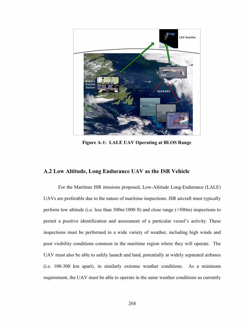
268
A.2 Low Altitude, Long Endurance UAV as the ISR Vehicle
For the Maritime ISR missions proposed, Low-Altitude Long-Endurance (LALE)
UAVs are preferable due to the nature of maritime inspections. ISR aircraft must typically
perform low altitude (i.e. less than 300m/1000 ft) and close range (<500m) inspections to
permit a positive identification and assessment of a particular vessel’s activity. These
inspections must be performed in a wide variety of weather, including high winds and
poor visibility conditions common in the maritime region where they will operate. The
UAV must also be able to safely launch and land, potentially at widely separated airbases
(i.e. 100-300 km apart), in similarly extreme weather conditions. As a minimum
requirement, the UAV must be able to operate in the same weather conditions as currently
LE O S ate llite
G round
C ontro l
S tation
U A V
S E N S O R S
Figure A-1: LALE UAV Operating at BLOS Range
269
flown by manned aircraft, if they are to be considered as an enhancement to manned
aircraft capabilities.
The LALE UAV is also a preferred platform for extended duration (i.e. over 12
hour) missions over large land areas, such as wildlife surveys and forest fire monitoring,
due to their ability to maintain extended presence on station. They typically have flight
endurance many times that of equivalent manned aircraft, and are able to fly lower and
slower then what would be considered safe for manned aircraft. Since they are
autonomous (i.e. have autopilots) they can follow a very precise “terrain hugging”
altitude profile for very long durations – well beyond the endurance limit for most human
pilots.
A.3 Outline of a Typical ISR Mission
The typical Maritime ISR mission to be performed by a LALE UAV may be divided
into several phases:
1. Launch – lift-off of the UAV at an airstrip.
2. Cruise to patrol area (1-2 hours).
3. Loiter in patrol area (8+ hours).
4. Inspect target(s) – as needed during loiter in area, tasked from shore-based GCS or
from local mobile airborne GCS. Duration of each would be a few minutes, with
possibly many (5+) each hour.
5. Return cruise to base (1-2 hours).
6. Landing.
Current operational UAVs can only be operated in a Waypoint Following (WF)
mode or Manual Pilot (MP) mode. In WF mode, the UAV autonomously follows a set of
270
GPS waypoints that are pre-programmed into the UAV before launch or dynamically
uploaded from the GCS while the UAV is in flight. The UAV relies on maintaining a
continuous GPS signal during this mode of navigation. Phases 2 and 5 would make
extensive use of this method of navigation. Phase 3 would likely use a special form of
WF available to most LALE UAVs, which allows the UAV to “orbit” a waypoint at a
certain distance and for a specified duration.
WF mode may be used during Phase 4 but only in limited cases, as the accuracy of
this navigation mode does not allow the precision necessary for successful close
inspections of moving vessels. Severe weather conditions may impact the availability and
integrity of the GPS signal. High winds could reduce the accuracy of WF course tracking
to the point where small UAVs may be blown off course by as much as 50-100 m, to the
point where it may pose a collision hazard to the target vessel. It was quickly realized
that some form of active guidance system would be needed during Phase 4, possibly using
visual or radar-based tracking similar to that used by guided missile seekers. Such a
guidance system must be able to operate in conditions of low visibility and to track
moving targets of interest, typically ships, to a fair level of accuracy (<30 m). It was
planned to combine this feature with an active DSA system to reduce the danger of
collisions with ground obstacles (including the target being inspected) and other airborne
vehicles.
In Manual Pilot (MP) mode, the vehicle is under real-time control by an operator. It
was noted that most operational UAVs use some form of MP during launch and landing
(Phases 1 and 6). In one configuration, the operator sits at a remote console at the
GCS. The operator relies on video and instrument data from the UAV, operating the
271
vehicle as if in the cockpit of the UAV. This is sometimes referred to as Virtual Piloting
(VP), or by the more current term FPV flying. This method requires very high quality
video camera imagery with little or no signal delay. In a more basic configuration, an
External Pilot (EP) remotely controls the UAV using standard radio-control (R/C)
equipment and methods, while standing at the side of the airstrip during take-off and
landing operations, relying on his or her natural eyesight to control the small aircraft.
This “third person view” mode is the most common method used for small LALE UAVs.
A.4 Experience with the Aerosonde UAV
A small fleet of Aerosonde UAVs were acquired in 2006 to be used to test the basic
utility of using this type of LALE UAV in the proposed ISR role. Detailed specifications
for the model purchased, the Mk4.2, may be found in Appendix B (Aerosonde AAI,
2006). Training and field operations were conducted from Fall 2006 until Summer 2008.
It soon became clear that while the Aerosonde UAV was capable of extreme endurance
(i.e. 24+ hrs) the limited payload, high cost of operation, and high attrition rate of
airframes soon defeated any attempt to use it in the originally proposed ISR role.
Increasingly restrictive rules being applied by TC at the time also served to curtail BLOS
operations (TC, 2010; TC UAV Working Group, 2007), to the point where flight
operations were restricted to basic circuit work within a kilometer of the runway.

272
Appendix B – Aerosonde Specifications
Table B-1: Aerosonde Technical Details (Aerosonde AAI, 2006)
Specification
Weight 13 - 15 kg (28.6 to 33 lb)
Max Take-off Weight 15 kg (33 lb)
Wing span 2.9 m (9.5 ft)
Engine 24 cc, Avgas, 1kw, Single Cylinder, Fuel Injected,
Premium Unleaded Gas
Fuel Consumption 180g/hr level flight
Min/Max Fuel 1.0 – 5.5 kg (1.2 – 6.5 L)
Navigation GPS/DGPS
UHF Communication Range 200 km depending on height and terrain
On board power generation 40 Watts continuous, 75 Watts peak, 18V DC
Payload Computer Supports Serial, Interface Input
Main Payload Bay Area (can be adapted) 100 mm Length, 120 mm Width, 180 mm Depth
Performance
Speed 18 – 32 m/s (49 to 62 Knots)
Endurance ~ 30 Hrs (All Fuel Payload)
~ 5 Hrs (Max Payload, Min Fuel)
Max Range ~ 2000 n.mi (All Fuel Payload)
~ 300 n.mi (Max Payload, Min Fuel)
Altitude Range 100 m to 6000 m
Payload Maximum 5 kg (approx 10-hour flight)
Mk 3 Payload Up to 4 kg (8.8 lb)
Mk 4.1 Payload Up to 6 kg (13.2 lb)
Landing & take off distance Less than 300 m
Take off speed Average 90 km/hr
Launch Vehicle Roof Rack & Catapult
Recovery Skid
Temperature +43ºC to -34ºC (+110ºF to -30ºF)
Operations
Staff for Launch and Recovery 3 People (Controller, Engineer, Pilot/Maintenance)
Staff for Flight Command 1 Person for several aircraft
Ground Equipment Proprietary Staging Box, 2 PCs, GPS
Flight Fully autonomous, or under Base Command.
Ground & Air communications UHF or Satellite (Iridium) to/from Aerosonde
Improvements in Mk4.1
Payload Mass 20% payload increase to 6 kg maximum
Payload Volume 30% payload volume increase
Endurance 20% endurance increase to more than 36 hours.
Engine/Powertrain The new power train system, based around Aerosonde's
proven electronic fuel injected engine, now provides a
dedicated payload supply with a 75W continuous
capability. A separate 40W supply is provided for use
by the guidance system.
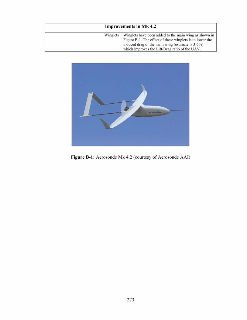
273
Improvements in Mk 4.2
Winglets Winglets have been added to the main wing as shown in
Figure B-1. The effect of these winglets is to lower the
induced drag of the main wing (estimate is 3-5%)
which improves the Lift/Drag ratio of the UAV.
Figure B-1: Aerosonde Mk 4.2 (courtesy of Aerosonde AAI)
274
Appendix C – Canadian Aviation Regulations
The following sections give an overview of the Canadian Aviation Regulations
(CARs), with an emphasis on the rules governing the most important aspects related to
the operation of UAVs in both controlled and uncontrolled airspace. It should be noted
that with minor exceptions, much of the CARs mirror a similar set of rules in other
countries, especially those of the FAA in the United States.
C.1 Airspace Classifications
C.1.1 Domestic Airspace Regions
Canadian Domestic Airspace is broadly classified into two large areas: the
Northern Domestic Airspace (NDA) and Southern Domestic Airspace (SDA) regions.
The NDA corresponds to the region of Canada where magnetic compasses are unreliable
due to the proximity of the north magnetic pole. In this region, aircraft headings, surface
wind directions and runway numbers are based on true north bearings. The NDA is also
where standard barometric altimeter setting (i.e. 29.92” Hg) is to be used. The NDA is
divided at approximately 72º latitude into the Northern Control Area and Arctic Control
Area for definition of the lower limit of controlled high altitude airspace.
The SDA is the southern area of Canada, where most of the population and
civilian airfields exist. In the SDA, magnetic compasses are useful, albeit with a known
declination correction between true north and magnetic north. Aircraft headings, wind
directions and runway headings are given relative to magnetic north. In the SDA, below
flight level FL180, altimeters are set to local barometric settings of airports during
275
landings and takeoffs, and updated as the aircraft passes within range of other barometric
stations en-route. The UAV flight activities by the majority of UAV operators in Canada
(including Project RAVEN) have been in the SDA region.
C.1.2 Controlled Airspace (Classes A-E)
The airspace classification system (i.e. Classes A through G) used in Canada
follows a similar format used worldwide. A common summary is the “inverted wedding
cake” diagram as shown in Figure C-1. This diagram attempts to summarize and simplify
the various classes of airspace, although anecdotal comments from some pilots suggest it
probably just adds to the already confusing array of rules which are contained within the
CARs. An attempt will be made here to summarize the various classifications in terms
important to small UAV operations.
Class A airspace is high altitude airspace where only Instrument Flight Rules
(IFR) flight is allowed. It is all airspace above 18,000 ft in the Southern Domestic
Airspace zone, and includes the high altitude air routes used by high speed civil transport
aircraft (i.e. airliners). All aircraft are expected to be equipped with radios, transponders,
and TCAS. In the Northern Domestic Airspace region, the altitude “floor” is FL230 in
the Northern Control Area and FL280 in the Arctic Control Area. Visual Flight Rules
(VFR) flight is prohibited in Class A airspace. Small UAV operations are unlikely in
Class A airspace.
Class B airspace is high altitude controlled airspace between 12,500 and 18,000 ft
ASL. To operate in Class B airspace, an aircraft must have a Mode C Transponder and
must establish two-way radio communications with Air Traffic Control (ATC). VFR
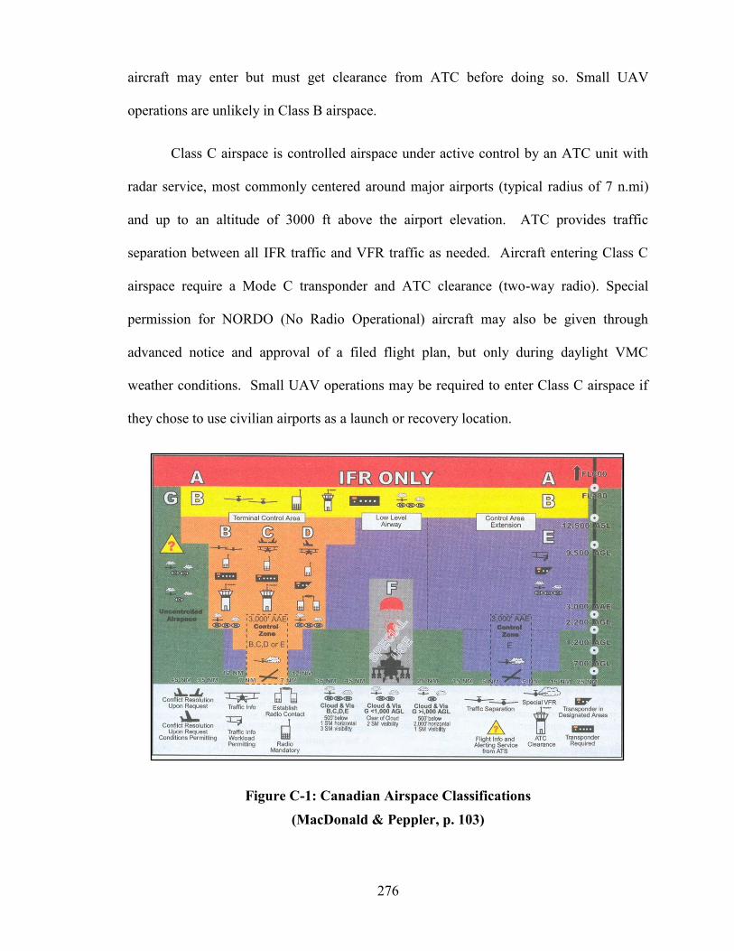
276
aircraft may enter but must get clearance from ATC before doing so. Small UAV
operations are unlikely in Class B airspace.
Class C airspace is controlled airspace under active control by an ATC unit with
radar service, most commonly centered around major airports (typical radius of 7 n.mi)
and up to an altitude of 3000 ft above the airport elevation. ATC provides traffic
separation between all IFR traffic and VFR traffic as needed. Aircraft entering Class C
airspace require a Mode C transponder and ATC clearance (two-way radio). Special
permission for NORDO (No Radio Operational) aircraft may also be given through
advanced notice and approval of a filed flight plan, but only during daylight VMC
weather conditions. Small UAV operations may be required to enter Class C airspace if
they chose to use civilian airports as a launch or recovery location.
Figure C-1: Canadian Airspace Classifications
(MacDonald & Peppler, p. 103)
277
Class D airspace is controlled airspace around smaller airports (typical radius of 5
n.mi) and up to 3000 ft AGL. To enter, aircraft must obtain ATC clearance. A
transponder may be required in some areas although most Class D control towers do not
have radar services. Small UAVs may need to enter Class D airspace if they operate
near or in/out of a smaller airport.
Terminal Control Areas are the “inverted wedding cake” shaped zones centered on
airports with ATC facilities, as seen in Figure C-1. The intent is to provide organized IFR
coverage at increasing flight altitudes at gradually increasing ranges from the airport. It
should be noted that at a particular range from an airport, an aircraft may be in
uncontrolled airspace, even though controlled airspace exists above some altitude. VFR
traffic may operate at the lower altitude without contacting ATC, but must contact ATC
and get clearance before climbing into the overlaying controlled airspace. Care must also
be taken to prevent inadvertent entry into controlled airspace due to horizontal travel (i.e.
moving closer to the airport).
Class E Airspace are areas where controlled airspace is needed at extended ranges
and altitudes from airports. Examples include lower-level airways, airport control zones,
transition areas, and extended approach paths used by commercial airline aircraft when
approaching busy airports. There are no special requirements for VFR aircraft to enter,
however certain areas (especially the control extension zones around some airports) will
require the mandatory use of two-way radios and Mode C Transponders. Most Class C
and D airspace zones revert to Class E when ATC services are shut down at a particular
airport. During RAVEN UAV operations on Bell Island, we were operating underneath

278
and to one side of one of the Class E extensions out of St. John’s International Airport. In
these situations, great care is taken to limit operational altitudes so as not to inadvertently
enter controlled airspace, as this could represent a risk to commercial airline traffic.
C.1.3 Restricted Airspace (Class F)
Class F Airspace is restricted airspace - areas where flight activities must be
confined and where non-participating aircraft operations must be restricted, either for
safety or national security reasons. Permanently established zones are marked on air
navigational charts, and identified (in Canada) by the letters CY, and a letter designating
the areas as either an (A)dvisory, (R)estricted, or (D)anger zone. Advisory areas are
zones where non-participating aircraft are warned to avoid or else exercise extra vigilance
to ensure safety. Restricted areas are (most commonly) zones used by the military for
flight tests and training exercises. Danger Zones are also defined in some areas. These
are restricted areas where special military testing (including live fire exercises) may occur
– which pose an obvious danger to any unexpected or unauthorized aircraft. Temporary
restricted airspace may also be established by being granted a SFOC which also triggers a
NOTAM to warn pilots of restrictions due to unusual activities in an area. This includes
all UAV flight testing undertaken by Project RAVEN since 2006. Note that in the current
regulatory environment, this is currently the only legal method by which UAVs are
permitted to operate in Canada (TC, 2010).
C.1.4 Uncontrolled Airspace (Class G)
All other airspace (i.e. not Class A-F) is considered uncontrolled Class G
Airspace. This encompasses a very large area, especially in the sparsely inhabited regions

279
common to Canada. Offshore areas are also largely uncontrolled. A LALE UAV is likely
to spend most of its operational life in Uncontrolled Airspace. Neither a transponder or 2-
way radio is mandatory when operating solely within Class G airspace. The possibility of
encountering such NORDO aircraft, which are by their nature non-cooperative versus any
transponder-based anti-collision system, represents a significant risk to routine UAV
operations.
C.2 VMC Rules (sighting distances)
The visual sighting minima applicable to Visual Meteorological Conditions
(VMC) are summarized in the following excerpts from the flight training manual “From
the Ground Up” (MacDonald & Peppler, p. 115). These excerpts summarize the visibility
regulations as contained in the Canadian Aviation Regulations (TC CARs, Part 6, Section
602.114 through 602.117, 2014):
Within Controlled Airspace:
Flight and Ground Visibility: not less than 3 miles
Height above surface: 500 ft minimum (1000 ft over built-up areas)
Distance from clouds: 500 ft vertically, 1 mile horizontally
Within Uncontrolled Airspace (at or above 1000 ft AGL):
Flight Visibility by Day: Not less than 1 mile
Flight Visibility by Night: Not less than 3 miles
Distance from clouds: 500 ft vertically, 2000 ft horizontally
Within Uncontrolled Airspace (below 1000 ft AGL):
Flight Visibility by Day: Not less than 2 miles

280
Flight Visibility by Night: Not less than 3 miles
Height above surface: 500 ft minimum (1000 ft over built-up areas)
Distance from clouds: Clear of Clouds
C.3 Aircraft Right-of-Way Rules
The basic Right-of-Way rules for aircraft are based on their relative ability to
maneuver (i.e. to avoid a collision). Therefore, priority is given in this order:
1. Balloons
2. Gliders
3. Airships
4. Aircraft towing another aircraft (i.e. glider tugs)
5. Powered aircraft (airplanes and helicopters)
When two aircraft are travelling in the same direction but on converging paths, the
aircraft to the right has priority. Similarly, any aircraft that is in the process of overtaking
another aircraft should maneuver such that it passes to the right and “well clear” of the
slower aircraft. A minimum distance of 500 feet is required, and fulfills the minimum
distance criteria from any person, vessel, vehicle or obstacle. In the case of a head-on
situation, the rule is to always turn to the right (i.e. both turn right, thus away from each
other). If two aircraft happen to be approaching to land on the same runway, a situation
which should be prevented with proper ATC, the aircraft at the higher altitude must give
way to the lower aircraft. Similarly, powerless aircraft (gliders) have priority over
powered aircraft trying to land on the same airstrip.
281
In any case, no matter what equipment, safety features or maneuverability that an
unmanned aircraft may possess, manned aircraft will likely always be considered as
having Right-of-Way over UAVs, which are generally regarded as “expendable” in the
context of manned aviation safety. It is currently the rule in SFOCs issued for UAV
flights in Canada that “the unmanned aerial vehicle shall give way to manned aircraft”
(TC, 2010). Even amongst USAF researchers, suggestions have been made to define a
specialized version of the “Robotic Laws” (after Isaac Asimov), applicable to UAVs
(“Flybots”). While self-preservation is to be considered (Third Law), this is overridden
by the First Law which forbids a Flybot from causing harm to another aircraft either by
direct action, or inaction. Thus, the UAV would sacrifice itself should the need arise, in
order to avoid harm to a manned aircraft (Barfield, 2000).
C.4 Traffic Separation Rules
C.4.1 Vertical Separation
Normal cruising altitudes for aircraft have been assigned in Canada, depending on
the direction of flight and whether an aircraft is flying by VFR or IFR. Easterly IFR
traffic (defined as having headings from 000º to 179º inclusive), are assigned to odd 1000
ft increments while westerly traffic is assigned to even 1000 ft increments. VFR traffic is
offset from IFR traffic by 500 ft, starting at 3500 ft. These altitudes ensure a minimum of
1000 ft vertical separation between opposing IFR traffic below FL290, and 2000 ft
separation above FL290. VFR traffic will likewise be separated 1000 ft from opposing
VFR traffic, but 500 ft from opposing IFR sharing the same airspace (below 18000 ft).
When VFR traffic is flying in Class B airspace (e.g. high altitude airways) they use the

282
same flight altitudes as IFR. There is no requirement for VFR below 3500 ft to adhere to
these guidelines, although the prudent pilot will still follow the odd/even IFR altitude plus
500 ft offset rule.
C.4.2 Horizontal Separation
There are a host of horizontal separation standards which are defined in the CARs
to ensure safe separation of traffic under ATC control (TC CARs, Part 8, Standard 821,
2014). A companion to these standards is the ATC Manual of Operations, which
establishes a set of standard procedures to be used across Canada (NAV Canada, 1999).
An attempt to summarize all of these standards would be outside the scope of this
document. In general, these separation minima are designed around high speed civil
transport aircraft (i.e. with cruise speeds in excess of Mach 0.7), and thus well over the
VMC minimum sighting distances quoted earlier. Separation distances are usually given
in terms of time differences versus a fixed navigation point for aircraft following one
another down an airway. The shortest minimum is 5 minutes. Lateral separation is
usually given in units of nautical miles, and the lowest minima here is 5 n.mi (TC CARs,
Part 8, Standard 821, 2014).
An important exception is where traffic converges in terminal control zones
around airports. Here, separation as low as 2.5 n.mi may be approved in some cases
although 3 n.mi is more typical. A crucial element to these minima being safe is that
airspeeds are limited to a maximum of 250 knots at 10,000 ft ASL and below. Another
concern is the separation of departing and arriving traffic near airports, especially to avoid
a trailing aircraft from flying into the wake of another. The minima applicable in these
283
cases are at least 2500 ft horizontal separation (approximately ½ mile) or three minutes
separation, for arriving and departing aircraft using the same runway.
C.5 Minimum Altitudes (Ground Obstacles)
The regulations concerning minimum altitudes are defined in the CARS (TC
CARs, Part 6, Section 602.14 and 602.15, 2014) with the following Minimum Altitudes
and Distances:
(a) Over Built-up Areas: At least 1000 feet above the highest obstacle located
within a horizontal distance of 2000 feet from the airplane; and,
(b) Elsewhere, a distance of at least 500 feet from any person, vessel, vehicle or
structure.
It is interesting that there are exceptions to these regulations, termed “Permissible
Low Level Flight”. Lower altitude flight is permitted if an aircraft is performing services
under the authority of several government bodies, such as police work, search and rescue,
fire-fighting, administration of The Fisheries or Coastal Fisheries Protection Acts,
provincial or national parks, or for the purposes of flight inspections (TC CARs, Part 6,
Section 602.14 and 602.15, 2014). Note that much of the Maritime ISR functions
currently executed by contracted private manned aircraft (e.g. PAL aircraft) fall into
several of these categories, as would a LALE UAV doing a similar role.
In the case of extended range LALE UAV operations over land, common
applications include wildlife aerial surveys, aerial mineral prospecting and aerial mapping
missions, which are also noted in Section 602.15 as “Permissible Low Level Flight”.

284
Thus, the LALE UAV, especially since it is unmanned, may legally operate at very low
altitudes, provided that there is no hazard to persons or property. This is unlikely to be a
difficult requirement, given the remote nature of most of these proposed land-based uses
of the LALE UAV.
C.6 Aircraft Lighting Requirements
The regulations for light requirements for small UAVs are yet to be finalized.
However, indications are that they may be considered to fall under the category of “very
light aircraft” (VLA). This is the same category as, for example, the kit-built Murphy
Elite floatplane which has a wingspan of about 30 feet and maximum gross weight of
1800 lbs (Patterson AeroSales, 2007). Assuming that the VLA requirements will apply,
these may be summarized with reference to the CAR 523-VLA-1 (TC CARs, Part 5, 523-
VLA-1385 to 1401, 2014). These lighting requirements are described below and
summarized in Figure C-2:
C.6.1 Navigation/Position Lights
The following steady navigation (Position) lights must be carried:
a) Red Navigational Light – on left wing tip, projecting Aviation Red over an arc
from 0 deg (directly ahead) to 110 deg Counter-clockwise. The light must have
minimum intensity of 40 Candela (towards front) and 5 Cd when viewed from the
left side.
b) Green Navigational Light – Similar to the red light, but on right wing tip,
projecting Aviation Green.
285
c) White Position Light – On the tail, projecting backwards over a 140º arc. The
light must have a minimum intensity of 20 Cd over the entire 140º arc.
The intent is for these lights to be visible at least 2 miles from the primary viewing
angle. In the case of the wingtip lights, this is the aircraft viewed head-on, while for the
tail lights it is when viewed from behind. This allows other aircraft to estimate the
relative aircraft orientation. For example, if both the green and red lights are visible, the
aircraft must be heading straight for you. If just the white lights are visible you are
behind the aircraft, etc. These lights must also be visible above and below the horizontal
plane, according to a factor table specified in the CARs. The requirement definition is
intended to guarantee good visibility within +/-30º of the horizontal plane.
C.6.2 Anti-Collision (Strobe) Lights
If an aircraft is going to operate in IFR conditions, or anytime at night, an anti-
collision light system must be used (TC CARs, Part 5, 523-VLA-1385 to 1401, 2014).
There are a several possible configurations permitted, as shown in Figure C-2. Whatever
configuration is used, the anti-collision light system must provide 360º coverage in the
horizontal plane, as well as +/-75º coverage in the vertical plane. Some view angle
obstruction (i.e. caused by the aircraft structure) is allowed, provided the total obstruction
is below 0.5 Steradians. The anti-collision lights may be either aviation red or aviation
white lights, with an effective flash rate of between 40 and 100 per minute. The intensity
of the strobe must be at least 400 Cd over the 360º horizontal plane. The intensity in the
vertical direction may be dimmer, but cannot drop below 20 Cd at +/-30 to +/-75º.
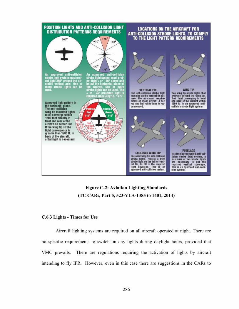
286
Figure C-2: Aviation Lighting Standards
(TC CARs, Part 5, 523-VLA-1385 to 1401, 2014)
C.6.3 Lights - Times for Use
Aircraft lighting systems are required on all aircraft operated at night. There are
no specific requirements to switch on any lights during daylight hours, provided that
VMC prevails. There are regulations requiring the activation of lights by aircraft
intending to fly IFR. However, even in this case there are suggestions in the CARs to

287
exercise caution when using anti-collision lights (strobes) when an aircraft is in thick
cloud or fog – as bright flashing lights have been known to cause problems with some
pilots. The pilot-in-command has the authority to turn the light system off, “where the
pilot-in-command determines that, because of operating conditions, doing so would be in
the interests of aviation safety” (TC CARs, Part 6, Section 605.17(2), 2014). However,
for the case of the small (and difficult to spot) LALE UAV, since there is no pilot
onboard that might be confused by exterior flashing lights, it would be more prudent to
leave the anti-collision strobe system on at all times.
C.7 Transponders
Transponders are required by aircraft which must fly within controlled airspace
(i.e. Classes A-C). Transponders may also be required in designed areas of Class D and E
airspace. According to ICAO regulations, the use of ACAS/TCAS II has been mandated
since 2005 for any aircraft above 5700 kg (12,600 lbs) and/or which will carry more the
19 passengers. This mandatory use of transponders and TCAS have resulted in a
significant improvement in safety, especially within the busy control zones around major
airports and along major air flight routes (ICAO, 2012, p. 3).
In contrast, the LALE UAV is likely to operate mostly in uncontrolled Class G
airspace, where there are no requirements for either radio communications or
transponders. This is one of the main issues regarding the integration of UAVs in civilian
airspace. There are also exceptions for Class D and E airspace, as well as the possibility
of NORDO aircraft in low-level Class G airspace. Unless there is a universal and
288
mandatory requirement for all aircraft to carry transponders, one cannot guarantee safety
through the use of transponder-based collision avoidance technologies.
C.8 Radio Use
The use of radio communication in aviation has become an indispensable tool, and
when used properly is a major contributor to the overall safety environment (MacDonald
& Peppler, p. 207). It is also a regulatory requirement that aircraft be equipped with a
minimum two-way radio capability (sometimes also called an “Airband Radio”) if they
plan to fly using IFR. It is also a requirement for VFR aircraft when they fly in controlled
airspace. These mandatory radio usage rules are noted in Figure C-1.
Radio communication is used in a two-way mode by ATC and aircraft to
coordinate air traffic, and also to provide regular traffic following services, especially for
high altitude commercial aircraft as they transitions from one control zone to another.
Smaller aircraft also benefit from such ATC guidance when within their control zone.
Local Tower radio control is used to coordinate take-offs and landings. All of this
requires precise radio call procedures both to and from various aircraft, as well as during
hand-offs from tower, to ATC, and to the next control zone.
Meanwhile, each pilot has the responsibility to properly respond and obey
ATC/Tower radio commands and to use regular radio calls, especially when approaching
airports or control zones where Mandatory Frequency (MF) rules are in place (RMC Inc.,
p. Section 4). The pilot is required to inform the ATC or Tower in advance of his arrival
in the aerodrome area, request proper landing/circuit directions and may also request
runway or weather reports. Regular calls are usually made as the pilot approaches and

289
enters the local traffic pattern, at regular intervals as he approaches to land, and when he
has cleared the runway, for example:
“Kilo Sierra Tango 5 mile southwest three thousand five hundred feet, inbound to
land”, “Entering Circuit”, “Established on Final”, “Clear of Runway”, etc.).
A similar set of calls are used when departing from an airport. It is normal to
request a runway for takeoff, wait for clearance, and to inform Tower when starting the
takeoff, and when the aircraft has successfully departed. The hand-off to ATC is handled
in a similar manner.
All of these regular radio calls serve a dual purpose – alerting and then updating
ATC on the progress of your aircraft, and also alerting other aircraft in the area of your
location and intensions. This contributes greatly to the overall situational awareness of all
of the nearby users of the aerodrome airspace.
The use of an Airband Radio follows a very specific standard for language and
usage. The universal language, by ICAO mandate, has been to use English as the primary
language when communicating with ATC. Standard phraseology and also the use of
phonetics for letters (e.g. “Alpha”, “Bravo”, “Charlie”) is used to provide the safest and
most effective communication, aiming to avoid confusion and also compensate for
mediocre radio reception. The use of such a radio requires that the operator hold the
appropriate license - in Canada this is Restricted Radiotelephone Operator’s Certificate.
Due to the flight training they receive, this by definition includes people having a valid
Pilot’s License. By reciprocal agreement this rules applies equally in in either Canada or
the U.S. (MacDonald & Peppler, p. 217)

290
It is noteworthy that radio usage is not mandatory if an aircraft flies in low-
altitude Class G. The presence of such NORDO aircraft in the modern aviation
environment is a little surprisingly. This exception is perhaps intended to allow the
occasional use of small “hobby aircraft” and also agricultural “crop dusters” without
requiring the apparently needless expense of equipping them with radios. However this
author has personally experienced the advantage to two aircraft operating in remote G
class airspace while using radios. In this situation, one of the pilots has the capability of
alerting the other to his presence (“I can see you”). It allows for the coordination of
landings at the many small single runway airstrips which dot the landscape across North
America. The prudent pilot will always equip his aircraft with a radio, and also a
transponder – to allow for the possibility that he may fly to a major airport. The small
UAV should likewise be similarly equipped.
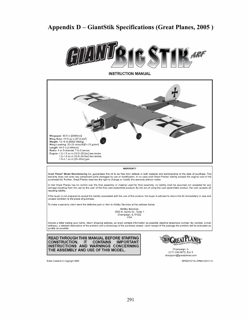
291
Appendix D – GiantStik Specifications (Great Planes, 2005 )

292
Appendix E – Autopilot Model
The following sections give a detailed description of the model developed to
represent the Autopilot (AP) used in the 4D Simulation Environment described in Chapter
5. The intent is to provide sufficient detail to permit the reader to understand how it was
implemented, and to allow replication of the methods used. Note that while the Picollo II
was the autopilot specifically simulated, the simulation is sufficiently generic to permit it
to represent any Proportional-Integral-Derivative (PID)-based autopilot which might be
used by a small UAV. Note that the extension of the AP to include active target guidance
was a novel addition by this author, as this is generally not a normal feature on any
current autopilots used for small UAVs.
E.1 Basic Autopilot Structure
A model of the Picollo II autopilot was developed in MATLAB/Simulink to
permit the accurate real-time simulation of typical Aerosonde UAV missions. The
development of this simulation was possible through detailed information contained in the
Picollo II technical documentation (CloudCap Technologies, 2006).
The basic autopilot structure may be seen in Figure E-1. The AP uses a set of
Outer Loop control laws, contained in the GNC Control block, to calculate the high-level
GNC commands. To keep the Simulink model neat most signals are multiplexed vectors,
each containing multiple parameters grouped into logical sets. For example, in the case
of GNC commands this is a triple of values representing the commanded Heading, Speed
and Altitude. These GNC commands are used, along with the current instantaneous UAV
state (i.e. angles, velocities, altitude) to drive a set of PID-based Inner Loops, contained in
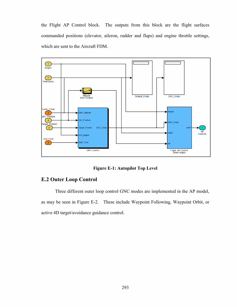
293
the Flight AP Control block. The outputs from this block are the flight surfaces
commanded positions (elevator, aileron, rudder and flaps) and engine throttle settings,
which are sent to the Aircraft FDM.
Figure E-1: Autopilot Top Level
E.2 Outer Loop Control
Three different outer loop control GNC modes are implemented in the AP model,
as may be seen in Figure E-2. These include Waypoint Following, Waypoint Orbit, or
active 4D target/avoidance guidance control.
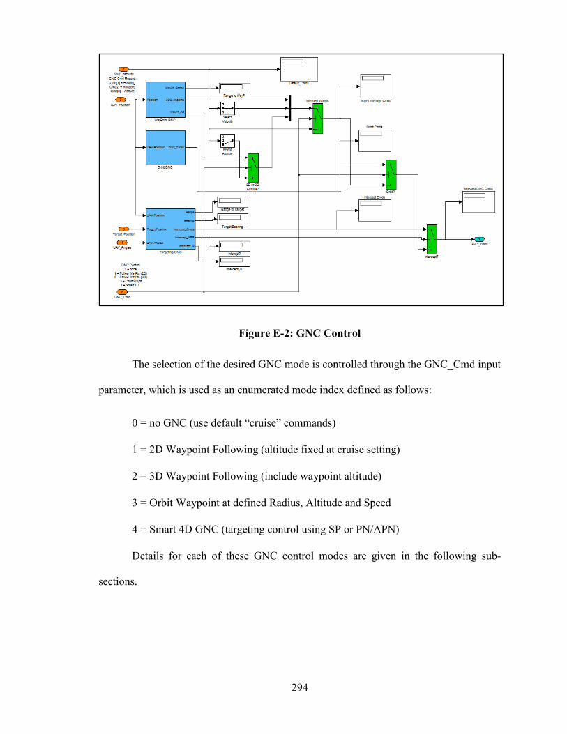
294
Figure E-2: GNC Control
The selection of the desired GNC mode is controlled through the GNC_Cmd input
parameter, which is used as an enumerated mode index defined as follows:
0 = no GNC (use default “cruise” commands)
1 = 2D Waypoint Following (altitude fixed at cruise setting)
2 = 3D Waypoint Following (include waypoint altitude)
3 = Orbit Waypoint at defined Radius, Altitude and Speed
4 = Smart 4D GNC (targeting control using SP or PN/APN)
Details for each of these GNC control modes are given in the following sub-
sections.

295
E.2.1 Waypoint Following
Figure E-3 shows the Waypoint Following control law which has been
implemented. The algorithm calculates the range and heading from the UAV location
(i.e. Position input) to the current waypoint position. All positions are defined in terms of
latitude, longitude and altitude above sea level. Built-in calculation blocks included with
the AeroSIM library are used to determine the distance between 3D points assuming an
earth-centered reference frame, and use of the WGS84 standard earth ellipsoid model
(Unmanned Dynamics, 2006). The waypoint selector block automatically cycles through
a pre-defined set of waypoints which are in sequence order. The waypoint selector
automatically switches from the current waypoint to the next one when the UAV position
comes within a minimum range of the targeted waypoint (i.e. typically 100m). 2D range
is used to define the required UAV heading (called LOC_heading) needed to intercept the
waypoint in a horizontal manner (i.e. latitude and longitude only). The waypoint altitude
is also set as the UAV commanded altitude if 3D waypoint following is activated.
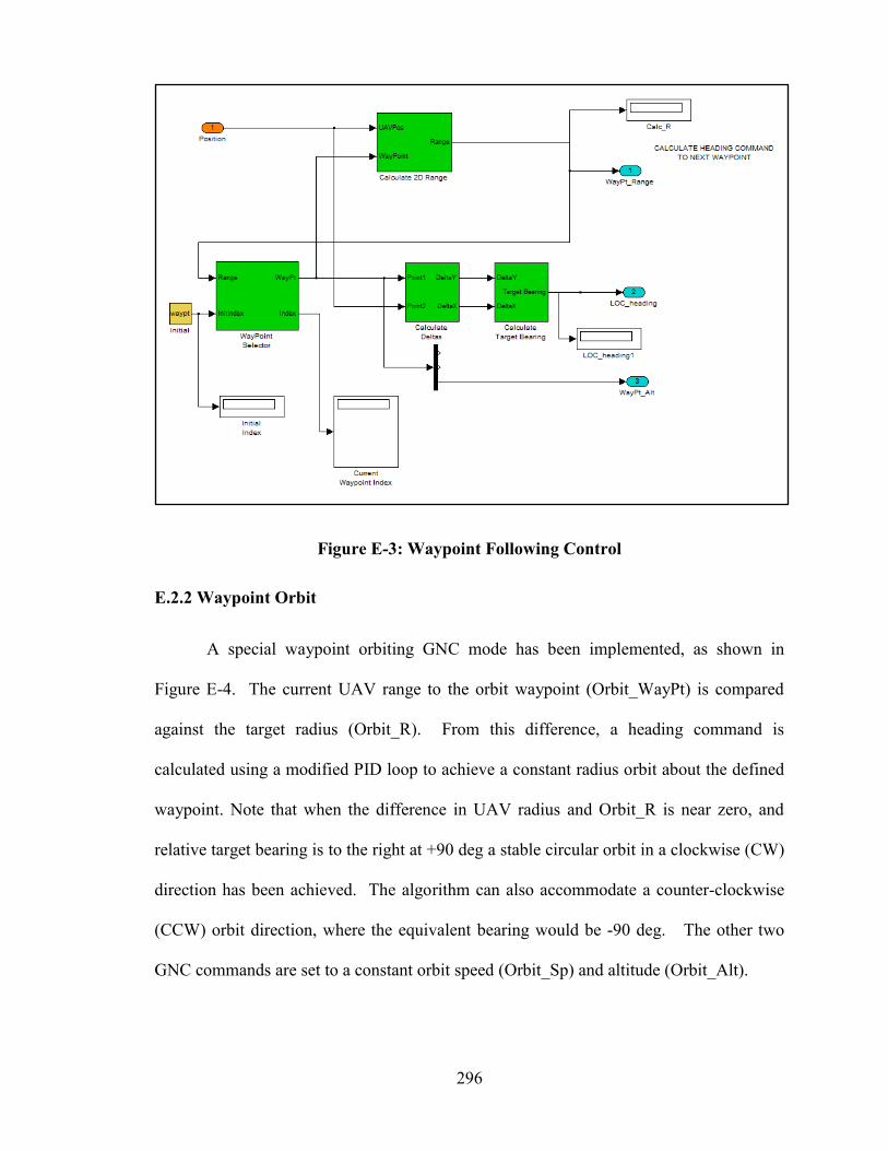
296
Figure E-3: Waypoint Following Control
E.2.2 Waypoint Orbit
A special waypoint orbiting GNC mode has been implemented, as shown in
Figure E-4. The current UAV range to the orbit waypoint (Orbit_WayPt) is compared
against the target radius (Orbit_R). From this difference, a heading command is
calculated using a modified PID loop to achieve a constant radius orbit about the defined
waypoint. Note that when the difference in UAV radius and Orbit_R is near zero, and
relative target bearing is to the right at +90 deg a stable circular orbit in a clockwise (CW)
direction has been achieved. The algorithm can also accommodate a counter-clockwise
(CCW) orbit direction, where the equivalent bearing would be -90 deg. The other two
GNC commands are set to a constant orbit speed (Orbit_Sp) and altitude (Orbit_Alt).
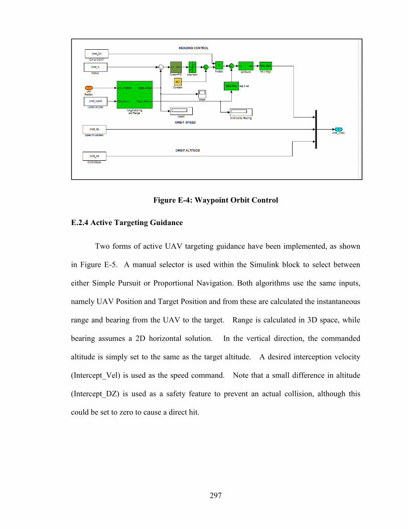
297
Figure E-4: Waypoint Orbit Control
E.2.4 Active Targeting Guidance
Two forms of active UAV targeting guidance have been implemented, as shown
in Figure E-5. A manual selector is used within the Simulink block to select between
either Simple Pursuit or Proportional Navigation. Both algorithms use the same inputs,
namely UAV Position and Target Position and from these are calculated the instantaneous
range and bearing from the UAV to the target. Range is calculated in 3D space, while
bearing assumes a 2D horizontal solution. In the vertical direction, the commanded
altitude is simply set to the same as the target altitude. A desired interception velocity
(Intercept_Vel) is used as the speed command. Note that a small difference in altitude
(Intercept_DZ) is used as a safety feature to prevent an actual collision, although this
could be set to zero to cause a direct hit.
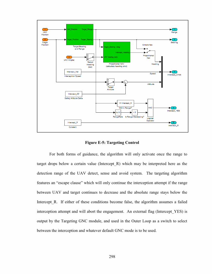
298
Figure E-5: Targeting Control
For both forms of guidance, the algorithm will only activate once the range to
target drops below a certain value (Intercept_R) which may be interpreted here as the
detection range of the UAV detect, sense and avoid system. The targeting algorithm
features an “escape clause” which will only continue the interception attempt if the range
between UAV and target continues to decrease and the absolute range stays below the
Intercept_R. If either of these conditions become false, the algorithm assumes a failed
interception attempt and will abort the engagement. An external flag (Intercept_YES) is
output by the Targeting GNC module, and used in the Outer Loop as a switch to select
between the interception and whatever default GNC mode is to be used.
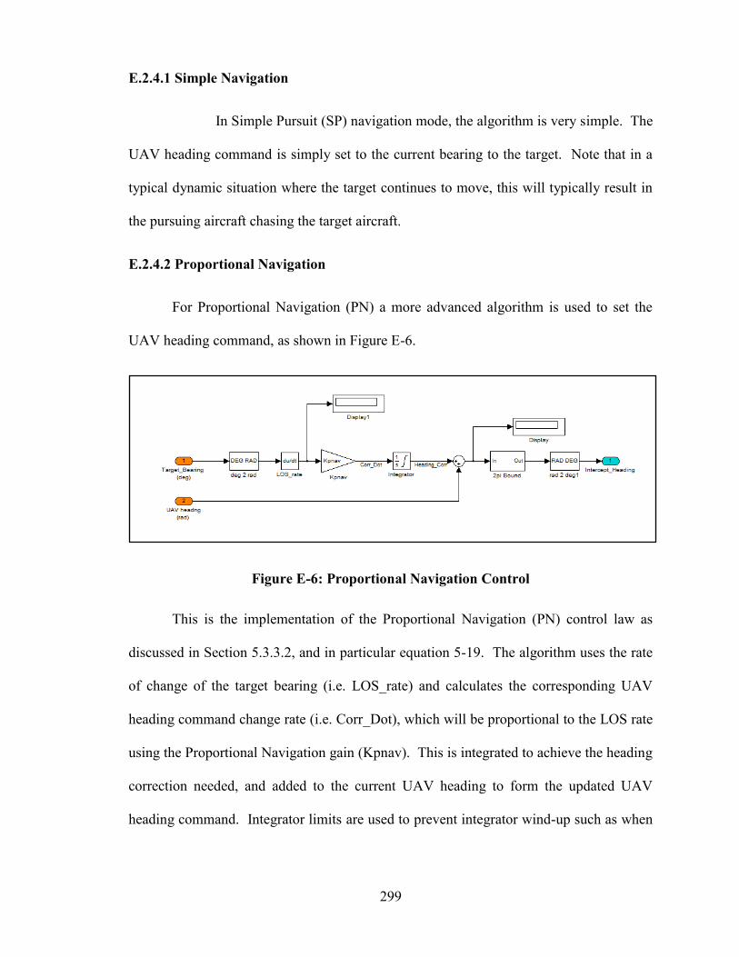
299
E.2.4.1 Simple Navigation
In Simple Pursuit (SP) navigation mode, the algorithm is very simple. The
UAV heading command is simply set to the current bearing to the target. Note that in a
typical dynamic situation where the target continues to move, this will typically result in
the pursuing aircraft chasing the target aircraft.
E.2.4.2 Proportional Navigation
For Proportional Navigation (PN) a more advanced algorithm is used to set the
UAV heading command, as shown in Figure E-6.
Figure E-6: Proportional Navigation Control
This is the implementation of the Proportional Navigation (PN) control law as
discussed in Section 5.3.3.2, and in particular equation 5-19. The algorithm uses the rate
of change of the target bearing (i.e. LOS_rate) and calculates the corresponding UAV
heading command change rate (i.e. Corr_Dot), which will be proportional to the LOS rate
using the Proportional Navigation gain (Kpnav). This is integrated to achieve the heading
correction needed, and added to the current UAV heading to form the updated UAV
heading command. Integrator limits are used to prevent integrator wind-up such as when

300
this algorithm should be dormant (i.e. range is outside the Intercept_R). When LOS rate
approaches zero, so will the heading correction rate. Assuming a properly tuned value of
Kpnav this should create the situation where the UAV will appear to lead the target,
which should result in a successful interception.
The forgoing discussion assumes a Proportional Navigation law, where the desire
is to intercept the target (i.e. create a 4D encounter). If a negative value of Kpnav is used,
this will have the opposite effect, and cause the aircraft to attempt to avoid the other
aircraft. A negative value of Kpnav results in heading corrections which will tend to
maximize the LOS rate between the interceptor and target.
E.3 Inner Loop Control
Inner loop controls are used to calculate the aircraft flight surfaces and throttle
settings needed to achieve the GNC commands calculated by the Outer Loop modes as
discussed previously. The overall structure may be seen in Figure E-7. In general, these
inner loops are simple PID-based control laws which dynamically adjust the various flight
controls in a closed-loop feedback control format to obtain these goals. The current UAV
body angles (angles), airstream velocities (VelAir) and altitude are used to in conjunction
with the GNC commands (GNC_Cmds) to calculate the corresponding errors in the UAV
attitude, airspeed and altitude, and from these the various control surface deflections and
throttle settings are determined.

301
Figure E-7: Autopilot Inner Loops
The Picollo II autopilot uses the concept of scaled PID gains in most of the PID
loops, to adjust the control behavior to the current flight speed of the UAV. This feature
is included in the AP model and follows the description provided in the Picollo II
technical manual (CloudCap Technologies, 2006). A reference dynamic pressure of 380
Pascals24
is used, based on the technical details provided in this reference and the gain
24 Dynamic pressure is Pdyn = ½ * air density * airspeed2. Assuming standard day and near sea level conditions, where air density is
approximately 1.2 kg/m3, a dynamic pressure of 380 Pascals corresponds to a forward airspeed of about 12.6 m/s.

302
definition for the Aerosonde UAV (Aerosonde AAI, 2006). Details for each of the
individual Inner Loops featured in the current AP model are as follows.
E.3.1 Heading from Roll (Aileron Control)
The commanded heading and UAV heading are compared, to determine the
heading error. A simple proportional gain is used to calculate the required bank angle.
This bank angle is limited to the aerodynamic limits of the airframe, and compared with
the UAV roll body angle to determine the roll error. Note that the inner PID control loops
for each of the primary flight controls (ailerons, elevator and rudder) are essentially
identical. The aileron loop is shown here as an example. Any major differences will be
noted in the next sub-sections.
Roll error is the primary driver for the aileron PID control loop, which is shown in
Figure E-8. As shown this is a modified PID control loop, with each of the gains scaled
by the reference dynamic pressure versus the actual UAV dynamic pressure. The
proportional term will be roll error multiplied by the scaled Kp. The integral term will
integrate the roll error and multiply this by Ki. The derivative term will be the current
first derivative of roll (i.e. roll rate) multiplied by Kd. These three terms are added
together to form the overall aileron flight surface command. A limit is applied as shown
in Figure E-7, which corresponds to the mechanical limits of the aileron deflection angle.
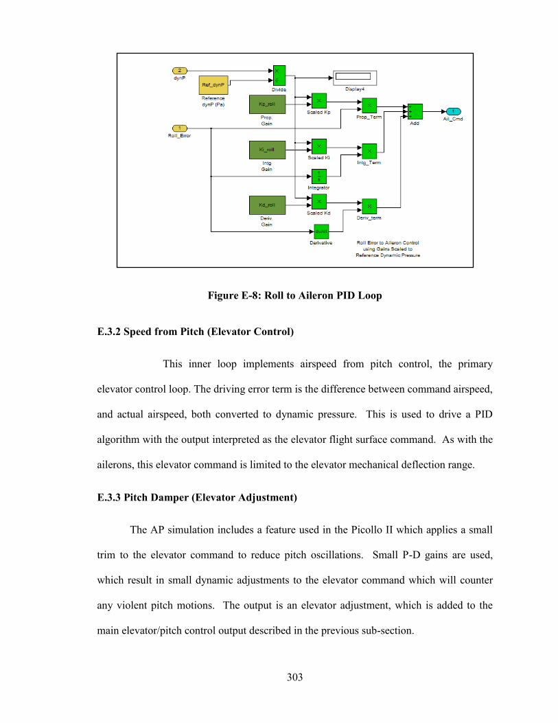
303
Figure E-8: Roll to Aileron PID Loop
E.3.2 Speed from Pitch (Elevator Control)
This inner loop implements airspeed from pitch control, the primary
elevator control loop. The driving error term is the difference between command airspeed,
and actual airspeed, both converted to dynamic pressure. This is used to drive a PID
algorithm with the output interpreted as the elevator flight surface command. As with the
ailerons, this elevator command is limited to the elevator mechanical deflection range.
E.3.3 Pitch Damper (Elevator Adjustment)
The AP simulation includes a feature used in the Picollo II which applies a small
trim to the elevator command to reduce pitch oscillations. Small P-D gains are used,
which result in small dynamic adjustments to the elevator command which will counter
any violent pitch motions. The output is an elevator adjustment, which is added to the
main elevator/pitch control output described in the previous sub-section.
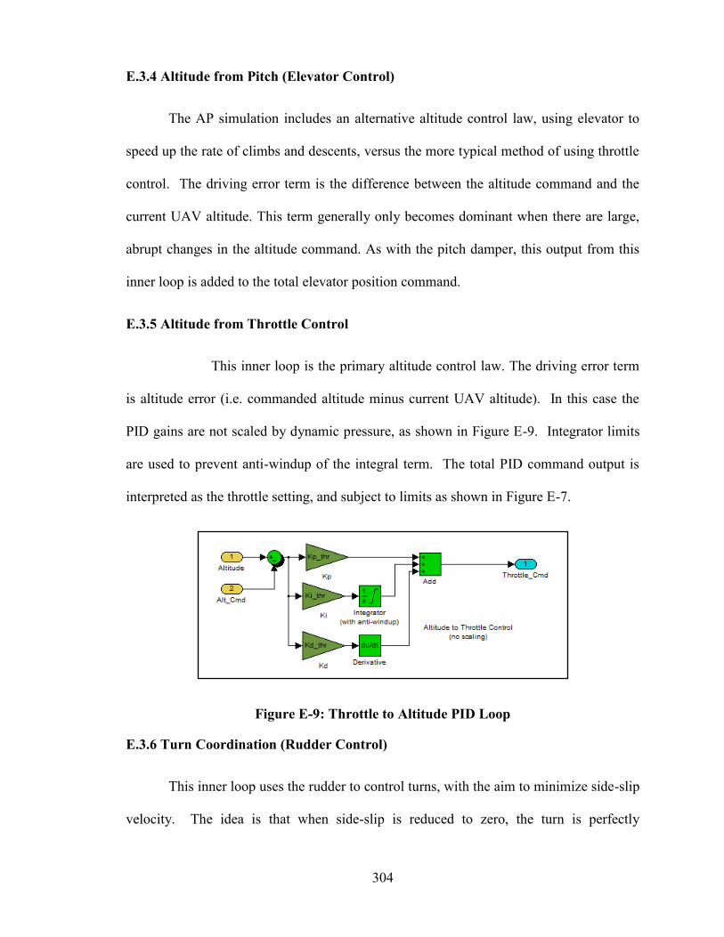
304
E.3.4 Altitude from Pitch (Elevator Control)
The AP simulation includes an alternative altitude control law, using elevator to
speed up the rate of climbs and descents, versus the more typical method of using throttle
control. The driving error term is the difference between the altitude command and the
current UAV altitude. This term generally only becomes dominant when there are large,
abrupt changes in the altitude command. As with the pitch damper, this output from this
inner loop is added to the total elevator position command.
E.3.5 Altitude from Throttle Control
This inner loop is the primary altitude control law. The driving error term
is altitude error (i.e. commanded altitude minus current UAV altitude). In this case the
PID gains are not scaled by dynamic pressure, as shown in Figure E-9. Integrator limits
are used to prevent anti-windup of the integral term. The total PID command output is
interpreted as the throttle setting, and subject to limits as shown in Figure E-7.
Figure E-9: Throttle to Altitude PID Loop
E.3.6 Turn Coordination (Rudder Control)
This inner loop uses the rudder to control turns, with the aim to minimize side-slip
velocity. The idea is that when side-slip is reduced to zero, the turn is perfectly
305
coordinated. Since the goal is zero, the error term is simply the current side-slip value,
assuming the use of negative PID gains. As with the throttle control loop, these PID
gains are not scaled so the internal PID algorithm is similar to as shown in Figure E-9.
The output of this inner loop is the rudder deflection angle command, which is limited to
the mechanical deflection limits of the rudder. This also drives a tail-wheel position for
the case of the GiantStik, but this has no effect on 4D simulation cases.
E.3.7 Flap Setting
This is a hold-over from when the simulation was used to develop automatic
takeoff and landing (ATOL) algorithms, where flaps are typically used. There is no
active flap inner loop in the 4D simulation. The flaps are simply set to a fixed scaled
value (i.e. 0-100% of maximum deflection angle) which for typical 4D simulations will
be zero (i.e. no flaps used).
306
Appendix F – Ethics Approval Materials
The Night-time VFR Light Experiment as documented in Chapter 4 was a human
factors experiment which involved the recruitment of human test subjects from both
within and outside the RAVEN project team. As such, the Interdisciplinary Committee
on Ethics in Human Research (ICEHR) review process in place at Memorial University
was followed. The ICEHR reference number assigned to this research project is
20140493-EN. This appendix is an archive of the ICEHR review and approval
paperwork applicable to this research project, as follows:
1. Ethics Review Approval Letter (September 20, 2013)
2. Signed Consent Form (Sample)
3. Renewal Request and Progress Report (September 26, 2014)
4. Application for Ethics Review (August 9, 2013)
The test procedure used during the experiment was included as an attachment in
the original Application for Ethic Review form. This is already detailed in Chapter 4 and
for the sake of brevity is omitted this Appendix.
As per ICEHR guidelines the originals of the Signed Consent Forms and notes and
data collections forms used during the experiment will be securely retained for a
minimum of five (5) years from the publication date of this thesis.

307
F.1 Ethics Review Approval Letter
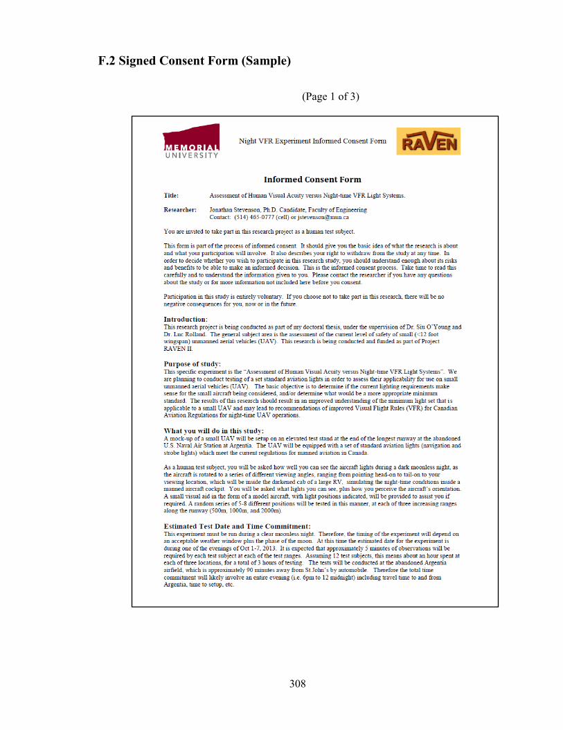
308
F.2 Signed Consent Form (Sample)
(Page 1 of 3)

309
(Page 2 of 3)
310
(Page 3 of 3)
311
F.3 Renewal Request and Progress Report
(Page 1 of 4)
312
(Page 2 of 4)

313
(Page 3 of 4)

314
(Page 4 of 4)
315
F.4 Application for Ethics Review
SECTION A – GENERAL INFORMATION
General instructions: This application form has been revised to facilitate the application and review process. It is designed to be completed and submitted electronically. Use the space inside the expandable textbox to provide the information requested. Please do not skip items. Answer “n/a” if it does not apply to your proposed research. Click or double - click on the “yes/no” box to select.
1. TITLE OF PROPOSED RESEARCH PROJECT
Assessment of Human Visual Acuity versus Night-time VFR Light Systems
b. PREVIOUS OR OTHER RESEARCH ETHICS BOARD
APPROVAL(S)
Has this research project been reviewed by another institution’s ethics board or another ethics board within
your institution?
Yes [Attach a copy of the application you submitted and the approval letter.]
Pending application Animal Care BioSafety [ please attach copies of
approvals]
No
Note: Research that has been reviewed and approved by another REB, please refer to Guidelines for
completing the proposal..
2. ORGANIZATIONAL OR COMMUNITY CONSENT If the research is taking place within a recognized organization or community (e.g. School Boards,
Band Councils, etc.) which requires that formal consent be sought prior to the involvement of individual
participants, explain whether consent from that organization/community will be sought. Describe this consent
process and attach a copy of the approval document. If consent will not be sought, please provide a
justification and describe any alternative forms of consultation that may take place.
N/A
3. STUDENT OR POST DOCTORAL FELLOW PRINCIPAL
INVESTIGATOR INFORMATION
Title: (Dr./Mr./Ms./etc)
Mr Last Name: Stevenson
First Name:
Jonathan Middle Initial:
D Department/Faculty/School (or Institution if not MUN):
Engineering Mailing address for correspondence, if different from
department/faculty/school:
Use Faculty of Engineering
MUN email address mandatory:
Telephone:
(514) 465-0777
MUN Student No.
008427577
316
Positions:
MUN Undergraduate Student MUN Master’s Student MUN PhD
Student
MUN Post-Doctoral Fellow Other (specify): Click here to enter text.
4. PROJECT PROGRAM
Undergraduate Honours Thesis Master’s Thesis Doctoral
Dissertation
Other: Click here to enter text.
5. CO-PRINCIPAL INVESTIGATOR INFORMATION (to be completed
if the project is being conducted by a group of students doing a group paper or
report) N/A
6. CO-INVESTIGATOR(S): [Do not include supervisor’s information here – see
item 6]
Name Position Faculty/Department Email
N/A
N/A N/A N/A
Click here to enter
text.
Click here to enter
text.
Click here to enter text. Click here to enter
text.
Click here to enter
text.
Click here to enter
text.
Click here to enter text. Click here to enter
text.
7. SUPERVISOR(S)
Name Department/Faculty/School (or Institution if not MUN) Email
Principal Supervisor:
Dr. Siu O’Young Engineering [email protected]
Co-supervisor:
Dr. Luc Rolland Engineering [email protected]
8. DATA COLLECTION START AND END DATES
Beginning of formal recruitment or informed consent process normally constitutes the start date of data collection.
Estimated project start date: 05-Aug-2013
Estimated start date of data collection involving human participants: 03-Oct-2013
Note – Please allow 4 weeks for review process, 6 weeks during peak periods.
End date of involvement of human participants is when all data has been collected from participants, no further contact
with them will be made, and all data are recorded and stored in accordance with the provisions of the approved
application.
Estimated end date of involvement of human participants for this project: 30-Nov-2013
Estimated project end date 31-Dec-2013
9. USE OF SECONDARY DATA

317
Does your project involve secondary use of data collected for other purposes? If it involves the use
of secondary data that is not in the public domain, provide letter of approval from the data holder.
Only secondary data
Both human participants and secondary data
Only human participants
10. FUNDING OF PROJECT
Is this project funded? No
Yes, funding agent/sponsor: ACOA/Project RAVEN II
If no, is funding being sought? No
Yes, funding agent/sponsor: Click here to enter text.
Will funds be administered through MUN? Yes No N/A
Funded research title if different from this application:
Project RAVEN II (ACOA funded)
Principal Investigator of above funded research: Dr. Siu O’Young
11. CONTRACTS
Is there a MUN funding or non-funded contract/agreement associated with the research? Yes No
If Yes, please include one (1) copy of the contract/agreement with this application
The full RAVEN-ACOA contract is undergoing amendment but is now available at the office of
the VPR (VP Research)
Is there any aspect of the contract/agreement that could put any member of the research team in a potential conflict of
interest? Yes No
If Yes, please elaborate under Section C, item #5.
12. SCHOLARLY REVIEW
The ICEHR will assume that research proposals prepared for presentation to the three national granting
councils (CIHR, NSERC and SSHRC), as well as other funding agencies, will be subjected to scholarly
review before funding is granted. The ethics review process for research that is beyond minimal risk will
incorporate a determination of the project’s scholarly merit and may request the researcher to provide full
documentation of such scholarly review.
Please check one:
The research project has undergone scholarly review prior to this application for ethics review by (specify
review committee – e.g. departmental research committee, peer-review committee, etc):
This experiment was presented in the Research Proposal presented at my Comprehensive Exam in Jan 2009.
The research project will undergo scholarly review prior to funding by (specify review committee – e.g.
departmental research committee, peer-review committee, etc):

318
Click here to enter text.
The research project will not undergo scholarly review.
The research project has been reviewed the supervisor(s).
SECTION B – SUMMARY OF PROPOSED RESEARCH
1. RATIONALE AND PURPOSE/RESEARCH QUESTION
Explain in non-technical, plain and clear language the purpose and objectives of the proposed project. Include
hypothesis or research question if applicable. The rationale for doing the study must be clear.
Maximum 1 page
The full experimental plan is attached to this application. The overall research project (PhD
project) is attempting to assess the equivalent level of safety aspects as related to unmanned
aerial vehicles (i.e. how to make them as safe or safer then manned aircraft). One of the aspects
is the sense and avoid aspects which includes the use of aviation lights to enhance the visibility
of an aircraft, especially at night or in adverse lighting/weather, to prevent collisions. The
specific research experiment in this application is focused on assessing the visual acuity of
typical human subjects at ever-increasing sight distances.
2. PROPOSED STUDY DESIGN/METHOD
Describe in some detail all procedures and methods to be used. Explain what the participants will be doing in
the study, types of information to be gathered from participants, where and how it will be obtained and
analyzed. If research includes intentions to publish, please indicate publication venues.
Attach a copy of all materials (survey questionnaires, interview questions, or other non-standard test
instruments) to be used in the study.
Maximum 3 pages
Please see the attached experimental plan. The basic procedure will be to have each human
subject seated inside a simulated night-time cockpit environment (inside the cab of an RV). A
small 10’ wingspan aircraft will then be presented to the test subject some distance away, with a
set of standard aviation lights attached. The aircraft will be rotated to present various angles of
sight (azimuth/heading) and the human subject will be asked to describe what they see and also
their estimate of the relative position of the aircraft based on the lights visible.
3. PARTICIPANTS INVOLVED IN THE STUDY
a. Indicate who will be recruited as potential participants in this study
Undergraduate students Graduate students Faculty or staff
General population Children Adolescents
Senior citizens Aboriginal people Other (specify): Click
here to enter text.
b. Specify the expected number of participants and exclusion criteria. Provide justification if
participation is dependent on attributes such as culture, language, religion, mental or physical disability,
sexual orientation, ethnicity, gender or age.
A minimum of 12 human subjects. At least half will be obtained from the current team
members of Project RAVEN, and to ensure a good mix of genders, their friends/partners.
319
The idea will be to dovetail the experiment proposed on existing plans to have the majority
of the team already at Argentia airfield. The test subjects will be identified in an
anonymous fashion, on the basis of gender, age and visual acuity (e.g. do they wear
glasses/contacts)
c. If your research involves Aboriginal peoples, please describe in detail the ethical issues relevant to
the proposed project and how you plan to comply with the TCPS2 guidelines Chapter 9.
N/A
d. Is there any pre-existing relationship between you (or any member of your research team) and the
participants (e.g. instructor-student; manager-employee)?
Yes No N/A
If yes, please explain:
As previously explained, most of the test subjects will be from the RAVEN team. This will include
using my supervisor(s) as test subjects too.
e. Are you or any member of your research team in a direct position of power to the participants
outside the scope of the research study?
Yes No N/A If yes, please explain:
My supervisors will be there as test subjects, but they are also a member of the research team
and thus some other members of the team are their students.
f. Will you or any member of your research team be collecting research data from your/their own
students?
Yes No N/A
If yes, please explain: My supervisors will be there as test subjects, but they are also a member of the
research team and thus some other members of the team are their students.
g. Will the targeted research population consist of any vulnerable group that will have difficulty
understanding or will not be able to give free and informed consent e.g. the mentally disabled, minors
(under 19), or any institutionalized individuals such as prisoners, etc?
Yes No
If yes, please explain:
N/A
4. RECRUITMENT PROCESS AND STUDY LOCATION a. Describe how, by whom, and from where the potential participants will be recruited. Where
participant observation is to be used, please explain the form of your (or members of your team)
insertion into the research setting (e.g. living in a community, visiting, attending organized functions).
Please make it explicit where it is reasonable to anticipate that all or some of the participants who will be
recruited will not speak English or will speak English as a second language. Describe any translation of
recruitment materials, how this will occur and whether or not those people responsible for recruitment
will speak the language of the participants. Attach a copy of any materials to be used for recruitment
[e.g., emails, posters, advertisements, letters, and telephone scripts].
Maximum 2 pages
Please see details in the research plan attached.
b. Identify where the study will take place.
On campus (e.g. university classroom, university lab, etc.) Please specify below.

320
Off campus (e.g. aboriginal community, schools, etc.) Please specify below.
Tests will be off-site at the abandoned Argentia Airfield.
5. EXPERIENCE For projects that involve collection of sensitive data, methods that pose greater than minimal risk to
participants, or involve a vulnerable population, please provide a brief description of your (or your research
team) experience with this type of research (including people who will have contact with the participants).
N/A
6. COMPENSATION If compensation is offered, it should not impose undue influence on a participant’s decision to participate in
the research. Justification for the amount of compensation to be offered should be provided.
a. Will participants receive compensation for participating in the research?
Yes No If yes, please provide details and justification for the amount or value of the compensation offered.
Participants will be volunteers from within the RAVEN Team and their partners.
b. If participants choose to withdraw, how will you deal with the compensation offered?
N/A
7. SHARING OF RESEARCH RESULTS WITH PARTICIPANTS
Explain what and how information/feedback will be provided to participants and/or communities after their
participation in the project is complete. (e.g., report, poster presentation, pamphlet, etc.)
A scientific paper and thesis chapter is expected to be the outcome of this research project.
RAVEN team members will of course we included in any invitations for lectures or presentation
of such results.
SECTION C – STATEMENT OF ETHICAL ISSUES
1. BENEFITS
a. Identify and describe any known or anticipated direct benefits to the participants (or to the
community) from their involvement in the project. Please do not list compensation as a benefit.
Within the RAVEN Team, the successful conclusion of this project may results in measurable
and new standards for light systems on UAVs and clear up the current confusion on whether to
equipt the UAVs with these lights, and if so, what configuration and type, etc.
b. Identify and describe any known or anticipated benefits to the scientific/scholarly community or
society that would justify involvement of participants in the research.
The outcome of this research is expected to be an updated set of HF data applicable to UAVs,
specific to night flying and UAV lighting standards. This will improve the safety of UAVs and
enhance their visibility.
2. HARMS
In explaining the risks involved in participating in a project, it is important to provide potential participants
with a clear understanding of the potential for harm. Research risks are those that reflect the likelihood and
magnitude of harms that participants may experience as a direct result of taking part in this research (e.g.,
stress or anxiety during data collection, stigma, loss of job, injury, etc.).
Please indicate if the participants as individuals or as part of an identifiable group or community might
experience any of the following risks by being part of this research project. In particular, consider any
factors that pose potential harm to at-risk groups.
321
a. Physical risks (including any bodily contact, administration of
any substance or in dangerous location such as politically unstable
countries)?
Yes No
b. Psychological/emotional risks (feeling uncomfortable,
embarrassed, anxious or upset)?
Yes No
c. Social risks (including possible loss of status, privacy or
reputation)?
Yes No
d. Is there any deception involved?
Yes No
e. Will your methods induce participants to act against
their wishes?
Yes No
f. Will participants be asked to disclose information of an
intimate nature or otherwise sensitive nature?
Yes No
g. Financial risks to participants (e.g. loss of job, promotion
opportunities, etc.)?
Yes No
h. Financial risks to organization/company (decrease in
demand for goods/services, loss of funding opportunities, etc.)?
Yes No
If yes to any of the above, please explain the risks and describe how they will be managed or minimized. In
the case of an adverse event (if any), provide information on how you plan to manage the risks inherent in
your research and provide information or resources to participants who might experience adverse effects
stemming from participation in your research.
The main physical risk involves the potential for accidents due to the need to travel from
St.John’s to Argentia after dark. Also, the tests involve a number of moves up/down the
main runway at Argentia, also in the dark.
The travel risk should be mitigated by organizing carpooling from St.John’s to Argentia to
minimize the need and number of vehicles used.
A large RV will be used both as the test “cockpit” and also as a means to house the human
subjects as they await their turn. The RV will also be used to move the human subjects
up/down the runway in a safe and quick manner.
The test itself is very simple and should not cause any stress, especially to anyone already
familiar with basic aviation lighting practise (i.e. red on left wingtip, green on right, white
tail lights, strobes, etc). A small visual aid in the form of a small model plane with the
various lights indicated will be available to assist anyone nervous or unsure about their
“expertise” in aviation light geometries.
3. FREE AND INFORMED CONSENT
You are encouraged to examine our informed consent form template for information on the required
minimum elements that should be included in the information letter and consent form, and follow a
similar format.
a. What process will you use to inform the potential participants about the study’s details and to obtain
the participants’ consent for participation? If the research involves extraction or collection of personally
identifiable information from a participant, please describe how consent from the individuals or
authorization from the data custodian will be obtained.
An “Informed Consent Form” will be used. This will adhere to the suggested ICEHR
format for such consent letters. A copy of the proposed Consent Form is included in this
review submission. In addition to serving as the written/signed consent form, it will serve
as the “Information Letter” for the study outlining the basic research plan, who the test

322
subjects will participate, what data will be collected and how it will be used. There will
also be a section used to collect basic test subject identification and contact information for
those who wish to participate. The only identification information collected will be gender,
age, nominal visual acuity (i.e. whether they wear vision correction like glasses/contacts)
and whether they have any aviation experience which might effect/bias there responses
during testing. Contact information (i.e. an email address) will be used to allow
coordination for the test date/time and travel arrangements, due to the unique nature of
the timing of these experiments (i.e. must be a clear dark moonless night).
b. If you will not be obtaining written consent, please provide the rationale for oral or implied consent
(e.g. discipline, cultural appropriateness, etc.) and explain how consent will be recorded. Also, explain
how you will ensure that participants understand that their participation is voluntary.
It is not expected that the volunteer nature of the participation of RAVEN team members
in one of their own team member’s PhD research will require significant problems with
regards to consent. The anonymous nature of how the human subjects will be identified
shouldn’t be a problem. However, a written and signed consent form will still be used for
ALL test subjects, and prepared/signed in advance, given the anonymous nature of how
each will be identified. This will also be helpful to explain the basic test procedure so
expectations once on the airfield are clear.
c. If the target population is not competent by reason of age or mental ability to provide free and
informed consent (the age of legal consent in this province is 19 years of age), describe and justify the
process you will use to obtain parental or third-party consent. [Note: If the participants are capable of
understanding the objectives and consequences of the research, their assent should be obtained in
addition to the consent of the parent or guardian.]
N/A
4. ANONYMITY OF PARTICIPANTS AND CONFIDENTIALITY OF DATA a. Describe the procedures you will use to protect anonymity of participants or informants, where
applicable, and the confidentiality of data during the conduct of the research and in the release of the
findings.
See previous comments.
c. Explain how written records, video/audio recordings, photographs, artifacts and questionnaires will
be securely stored, how long they will be retained, who will have access, and provide details of their
storage location and final disposal. Provide a justification if you intend to store your data for an
indefinite length of time. If the data may have archival value, discuss this and whether participants will
be informed of this possibility during the consent process. Data security measures should be consistent
with Memorial University’s Policy on Integrity on Scholarly Research .
Written records in the form of test recording sheets, and human subject identification forms will
be retained until the conclusion of the PhD research project. The intent is to have this as the
“raw data” until it is properly analysed and summarized and presented in the form of statistical
results (e.g. scatterplots). The results will become part of at least one chapter in my Thesis and
possibly also in a scientific paper. d. Describe any limitations to protecting the confidentiality of participants’ data (eg. access to or
disclosure of information during or at the end of the study) whether due to the law, the methods used or
other reasons (e.g. duty to report).
N/A
323
e. If participants’ anonymity is difficult or impossible to achieve (e.g. in focus groups), please explain
the limits to anonymity.
N/A
5. CONFLICT OF INTEREST If any member of the ICEHR is ineligible to review your application because of a conflict of
interest, please notify the ICEHR administrative staff.
If the proposed research involves real or apparent conflict of interest (e.g., yours or your team’s judgement
may be influenced or appear to be influenced by private or personal interests such as remuneration,
intellectual property rights, rights of employment, consultancies, board membership, stock options, etc.),
please identify and explain how you will inform research participants of these conflicts.
N/A
6. PARTICIPANT WITHDRAWAL
a. Please describe how participants will be informed of their right to withdraw from the project.
Outline the procedures which will be followed to allow them to exercise this right.
Participation in the experiment will be solely voluntary – drawing from individuals from
the team members and their friends/partners. A written consent form will be used. The
form will clearly state that given the logistics of gathering everyone at the remote test site,
it may not be practical (or safe) for test subjects to leave prematurely, once the test
procedure has started. The consent form will include a description of the test procedure
and the expected time commitment for each test subject so they can make an informed
decision to participate.
c. Indicate what will be done with the participant’s data and any consequences that withdrawal may
have on the participant.
N/A
d. If participants will not have the right to withdraw from the project at all, or beyond a
certain point, please explain.
Once the experiment is started, each test subject will be required to “see it through” and
complete each of their test points to completion. This will involve three sets of 5min
observations each, for a total of about 1 hour spent at each range location. This is to ensure
a valid set of data, especially for comparisons between the three sighting distances, and to
permit some statistical analysis. With the reduced number of human subjects (12) this is
especially important.
7. DECEPTION a. Describe and justify the use of deception or intentional non-disclosure in this study.
N/A
b. Explain and justify if information will be withheld from participants that might reasonably lead
them to decline to participate in the study.
N/A
324
c. Explain and justify if participants will be photographed or video- or audio-taped without their
knowledge or consent.
N/A
d. Debriefing (Attach a copy of written debriefing sheet or script) Outline the process to be used to debrief participants. Explain and justify whether participants will
be given the option of withdrawing their data following the debriefing.
No debriefing planned.
Recruitment Documents and Consent Forms A template of an Informed Consent Form is available on the ICEHR Website. The Committee encourages you to examine the template and follow a similar format. Note that the template outlines only the minimum information that should be included in an informed consent form. Please consult the ICEHR guidelines for additional information that may be required.
Note:
The ICEHR approval statement must be included on all recruiting information and consent forms given to participants, and should be in a paragraph separated from all other text or contact information.
A consent form checklist is provided to assist you to ensure you that you have covered everything necessary for your project.
Application Checklist (This checklist must be completed and included with your electronic application)
New application
HREA Notification Form (only for health related research) N/A
Resubmission as requested Forwarded e-copy of electronic application and attachments to [email protected]
Answered all questions on the application form Section D of Form 1B completed and signed by PI and supervisor and forwarded to ICEHR
The ICEHR Approval Statement included on Informed Consent Form and Recruitment Documents Where Applicable, Attachments Included with Application:
Proposed Recruitment letter, Advertisement, Poster (include in Consent Form) Proposed Questionnaire, Survey, or Other Instrument Proposed Interview Questions Proposed Oral Script for Recruitment (e.g., in-class and telephone invitation/information script) Proposed Information Letter for Participants (include in Consent Form) Proposed Informed Consent Form for Participants Proposed Information Letter for Parents, Guardians, Proxy Proposed Consent Form for Parents, Guardians, Proxy Proposed Debriefing Statement (if using deception) Other, please specify: Detailed TEST PLAN for experiment

325
SECTION D – SIGNATURE
TITLE OF PROPOSED RESEARCH PROJECT
Assessment of Human Visual Acuity versus Night-time VFR Light Systems
PRINCIPAL INVESTIGATOR:
As the Principal Investigator on this project, my signature confirms that I have read Memorial University’s Policy on
Ethics of Research Involving Human Participants and the Tri-Council Policy Statement on Ethical Conduct for
Research Involving Humans (TCPS2). I will ensure that all procedures performed under the project will be conducted
in accordance with the TCPS2 and all relevant university, provincial, national and international policies and regulations
that govern the collection and use of personally identifiable information in research involving human participants. I
agree to conduct the research subject to Section 3 (Guiding Ethical Principles) and accept the responsibilities as outlined
in Section 18 (Responsibilities of Researchers) of Memorial University’s Policy on Ethics of Research Involving
Human Participants.
Any deviation from the project as originally approved will be submitted to ICEHR for approval prior to its
implementation. I understand that deviations from the project that alter the risks to participants and that are
implemented without ethics approval constitute a violation of the TCPS2 and Memorial University’s policy.
If there is any occurrence of an adverse event(s), I will complete and submit Form 5 – Adverse Event(s) Report to the
Chair of ICEHR immediately.
My signature confirms that my project has been reviewed and approved by my supervisor(s) and advisory committee
(where applicable). If my status as a post-doctoral fellow/student changes, I will inform the ICEHR.
Click here to enter text.
Click here to enter text.
Name and Signature of Principal Investigator
Jonathan Stevenson
Date
PRINCIPAL SUPERVISOR:
As the Principal Supervisor of this project, my signature confirms that I have reviewed and approved the scholarly
and/or scientific merit of the research project and this ethics protocol submission.
I understand that as the Principal Supervisor, I have ultimate responsibility for the conduct of the study, the ethical
performance of the project and the protection of the rights and welfare of human participants. I will provide the
necessary training and supervision to the researcher throughout the project to ensure that all procedures performed
under the research project will be conducted in accordance with the TCPS2 and all relevant University, provincial,
national or international policies and regulations that govern research involving human participants.
I will ensure that any deviation from the project as originally approved will be submitted to the ICEHR for approval
prior to its implementation, and any occurrence of adverse event(s) will be reported to the ICEHR immediately.
Click here to enter text.
Name and Signature of Principal Supervisor
Dr. Siu O’Young
Dr. Luc Rolland
Date