assessment of the fluid-structure interaction … · vii european congress on computational methods...

ECCOMAS Congress 2016VII European Congress on Computational Methods in Applied Sciences and Engineering

M. Papadrakakis, V. Papadopoulos, G. Stefanou, V. Plevris (eds.)Crete Island, Greece, 5–10 June 2016

ASSESSMENT OF THE FLUID-STRUCTURE INTERACTIONCAPABILITIES FOR AERONAUTICAL APPLICATIONS OF THE

OPEN-SOURCE SOLVER SU2.

Ruben Sanchez1∗, H. L. Kline2, David Thomas3, Anil Variyar2, Marcello Righi4, ThomasD. Economon2, Juan J. Alonso2, Rafael Palacios1, Grigorios Dimitriadis3, Vincent

Terrapon3

1Department of Aeronautics, Imperial College LondonLondon, SW7 2AZ, United Kingdom

e-mail: r.sanchez-fernandez14, [email protected]

2 Department of Aeronautics & Astronautics, Stanford UniversityStanford, CA, 94305, USA

e-mail: hlkline, anilvar, economon, [email protected]

3 Department of Mechanical and Aerospace Engineering, University of LiegeLiege, 4000, Belgium

e-mail: dthomas, vincent.terrapon, [email protected]

4 School of Engineering, Zurich University of Applied SciencesWinterthur, 8401, Switzerland

e-mail: [email protected]

Keywords: Fluid-Structure Interaction, Computational Aeroelasticity, Reynolds-Averaged NavierStokes, Geometrically-Nonlinear Solid Mechanics

Abstract. We report on an international effort to develop an open-source computational en-vironment for high-fidelity fluid-structure interaction analysis. In particular, we will focus onverification of the implementation for application in computational aeroelasticity. The capabil-ities of the SU2 code for aeroelastic analysis have been further enhanced both by developingnatively embedded tools for the study of largely deformable solids, and by wrapping it usingPython tools for an improved communication with external solvers. Both capabilities will bedemonstrated on relevant test cases, including rigid-airfoil solutions with indicial functions,the Isogai Wing Section, test cases from the AIAA 2nd Aeroelastic Prediction Workshop, andthe vortex-induced vibrations of a flexible cantilever in the wake of a square cylinder. Resultsshow very good performance both in terms of accuracy and computational efficiency. The mod-ularity and versatility of the baseline suite allows for a flexible framework for multidisciplinarycomputational analysis. The software libraries have been freely shared with the community toencourage further engagement in the improvement, validation and further development of thisopen-source project.

Sanchez, Kline, Thomas, Variyar, Righi, Economon, Alonso, Palacios, Dimitriadis, Terrapon

1 INTRODUCTION

The interaction between fluids and structures on complex geometries is a challenging compu-tational problem that has attracted substantial interest due to its relevance across disciplines, in-cluding aeronautical and civil engineering, biomechanics, and turbomachinery. In this work, wewill focus on aeronautical applications, and particularly on computational aeroelasticity [1–3].Due to the complexity of the constitutive equations and the strongly non-linear coupling effectsbetween fluid and structure, the development of accurate and efficient solvers able to be runin highly-parallel environments becomes a determining factor, specially when addressing largeproblems that require refined discretisations.

With this in mind, the open-source software suite SU2 [4–6] has been used as the basicinfrastructure for the development of a set of tools for Fluid-Structure Interaction (FSI). Dueto its modularity and versatility, it has been possible to develop natively embedded tools fornon-linear structural analysis in SU2, thus allowing for a self-contained, open-source suite ca-pable to deal with FSI problems involving largely deformable solids [7]. At the same time, thesuite has been wrapped using Python tools for improved communication with external solvers,which increases the flexibility for the user when aiming to solve problems using other in-houseor commercial platforms. In this paper we will detail the modular implementations we haveincluded in SU2 in the context of FSI, and we will assess the validity of these methods.

The paper is organized as follows. Section 2 briefly describes the governing equations forfluid and structural mechanics, and establishes the interface coupling conditions. Section 3sketches the structure of the code for the fluid and structural solver, and the architecture that per-mits the coupling of the independent solvers with each other or with external tools via Python.Section 4 presents the first set of results obtained using the different approaches described. Fi-nally, section 5 summarizes the current state of the project and outlines some of the plannedfuture developments.

2 BACKGROUND

2.1 Fluid mechanics

2.1.1 Governing equations

We are concerned with compressible, turbulent fluid flows governed by the Reynolds-averagedNavier-Stokes (RANS) equations, which can be expressed in arbitrary Lagrangian-Eulerian(ALE) [8] differential form as

∂U

∂t+∇ · Fc −∇ · Fv −Q = 0 in Ω× [0, t] (1)

where the conservative variables are given by U = ρ, ρv, ρET, and the convective fluxes,viscous fluxes, and generic source term are

Fc =

ρ(v − uΩ)

ρv ⊗ (v − uΩ) + ¯IpρE(v − uΩ) + pv

, Fv =

·¯τ

¯τ · v + µ∗totcp∇T

, (2)

and Q = qρ,qρv, qρET, where ρ is the fluid density, v = v1, v2, v3T ∈ R3 is the flow speedin a Cartesian system of reference, uΩ is the velocity vector at a point for a domain in motion(mesh velocity after discretization), E is the total energy per unit mass, p is the static pressure,


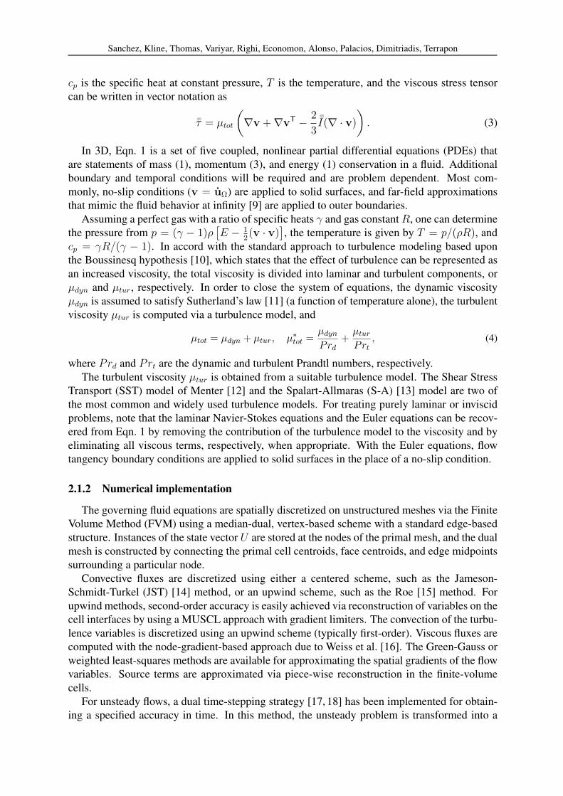
cp is the specific heat at constant pressure, T is the temperature, and the viscous stress tensorcan be written in vector notation as

¯τ = µtot

(∇v +∇vT − 2

3¯I(∇ · v)

). (3)

In 3D, Eqn. 1 is a set of five coupled, nonlinear partial differential equations (PDEs) thatare statements of mass (1), momentum (3), and energy (1) conservation in a fluid. Additionalboundary and temporal conditions will be required and are problem dependent. Most com-monly, no-slip conditions (v = uΩ) are applied to solid surfaces, and far-field approximationsthat mimic the fluid behavior at infinity [9] are applied to outer boundaries.

Assuming a perfect gas with a ratio of specific heats γ and gas constantR, one can determinethe pressure from p = (γ − 1)ρ

[E − 1

2(v · v)

], the temperature is given by T = p/(ρR), and

cp = γR/(γ − 1). In accord with the standard approach to turbulence modeling based uponthe Boussinesq hypothesis [10], which states that the effect of turbulence can be represented asan increased viscosity, the total viscosity is divided into laminar and turbulent components, orµdyn and µtur, respectively. In order to close the system of equations, the dynamic viscosityµdyn is assumed to satisfy Sutherland’s law [11] (a function of temperature alone), the turbulentviscosity µtur is computed via a turbulence model, and

µtot = µdyn + µtur, µ∗tot =µdynPrd

+µturPrt

, (4)

where Prd and Prt are the dynamic and turbulent Prandtl numbers, respectively.The turbulent viscosity µtur is obtained from a suitable turbulence model. The Shear Stress

Transport (SST) model of Menter [12] and the Spalart-Allmaras (S-A) [13] model are two ofthe most common and widely used turbulence models. For treating purely laminar or inviscidproblems, note that the laminar Navier-Stokes equations and the Euler equations can be recov-ered from Eqn. 1 by removing the contribution of the turbulence model to the viscosity and byeliminating all viscous terms, respectively, when appropriate. With the Euler equations, flowtangency boundary conditions are applied to solid surfaces in the place of a no-slip condition.

2.1.2 Numerical implementation

The governing fluid equations are spatially discretized on unstructured meshes via the FiniteVolume Method (FVM) using a median-dual, vertex-based scheme with a standard edge-basedstructure. Instances of the state vector U are stored at the nodes of the primal mesh, and the dualmesh is constructed by connecting the primal cell centroids, face centroids, and edge midpointssurrounding a particular node.

Convective fluxes are discretized using either a centered scheme, such as the Jameson-Schmidt-Turkel (JST) [14] method, or an upwind scheme, such as the Roe [15] method. Forupwind methods, second-order accuracy is easily achieved via reconstruction of variables on thecell interfaces by using a MUSCL approach with gradient limiters. The convection of the turbu-lence variables is discretized using an upwind scheme (typically first-order). Viscous fluxes arecomputed with the node-gradient-based approach due to Weiss et al. [16]. The Green-Gauss orweighted least-squares methods are available for approximating the spatial gradients of the flowvariables. Source terms are approximated via piece-wise reconstruction in the finite-volumecells.

For unsteady flows, a dual time-stepping strategy [17, 18] has been implemented for obtain-ing a specified accuracy in time. In this method, the unsteady problem is transformed into a


series of steady problems at each physical time step that can then be solved using all of thewell-known convergence acceleration techniques for steady problems. Each physical time stepis relaxed in pseudo time using implicit integration.

During time-accurate calculations on dynamic meshes, the coordinates and velocities of thegrid nodes must be updated at each physical time step using suitable methods for displacingthe nodes of the volume mesh and computing the resulting grid node velocities. Two typicalstrategies involve rigid mesh transformations or dynamically deforming meshes. In the former,the grid node coordinates and velocities are often computed analytically based on a prescribedmotion of the mesh as a rigid body. The dynamically deforming case, which is typically nec-essary for FSI problems, requires an additional technique to deform the fluid volume mesh toconform to specified changes in the positions of solid boundaries. After updating the positionof all nodes in the fluid mesh, the local grid velocity at a node can be computed by storing thenode coordinates at prior time instances and using a finite differencing approximation that isconsistent with the chosen dual time-stepping scheme.

Finally, when computing unsteady flows on dynamic meshes with the ALE form of theequations, a Geometric Conservation Law (GCL) should be satisfied. First introduced byThomas and Lombard [19], it has been shown mathematically and through numerical exper-iment [20–22] that satisfying the GCL can improve the accuracy and stability of the chosenscheme. A straightforward technique for the numerical implementation of the GCL [23,24] hasbeen included as part of the dual-time stepping approach.

2.2 Structural mechanics

2.2.1 Rigid body models

The following model can be considered for the constrained displacement of non-deformablebodies. The kinematics can be described by a finite set of degrees of freedom correspondingto a translation of body-attached point O and a rotation around this point. This is illustrated inFig. 1 where both an absolute frame of reference and a relative frame of reference attached tothe solid body (denoted by the ’ symbol) are considered. Initially, these two referential framesare superposed. After a displacement, the absolute position s of any point P within the solid canthus be written as [25]:

sP = sO + r′ = sO + Rr (5)

where sO is the translation of the reference point, r′ is the relative position of P in the body-attached frame of reference, r is the position of P before the displacement and R is a rotationmatrix.

The rotation matrix is based on the choice of the parametrization for the rotation and de-scribes the rotation of the relative frame of reference O’ in the absolute referential frame. Inthe case of a three-dimensional rotation, it can be separated into ordered rotations of angles θ,φ and ψ around the x, y and z-axis respectively, which gives the following rotation matrix:

R(θ,φ,ψ) =

cosφ cosψ sin θ sinφ cosψ − cos θ sinψ cos θ sinφ cosψ + sin θ sinψcosφ sinψ sin θ sinφ sinψ + cos θ cosψ cos θ sinφ sinψ − sin θ cosψ− sinφ sin θ cosφ cos θ cosφ

In the case where the rigid body displacement is dynamically constrained by some constant

stiffness or damping, Lagrange’s equation [26,27] can be used to build the equations of motion


O

O’

P

P

r

r’sO

sP

ex

ez

ey

ex

’

ey

’

ez

’

Figure 1: Vectorial description of a rigid body displacement, before (blue) and after (red) thedisplacement.

for an arbitrary number n (from one to six) of degrees of freedom uj:

d

dt

(∂T

∂uj

)−(∂T

∂uj

)+

(∂V

∂uj

)+

(∂D

∂uj

)= Fj(t) j = 1, · · · , n (6)

where T is the kinetic energy related to the mass and the inertia, V the potential energy relatedto the stiffness, D is the dissipation function related to the damping and Fj is the generalizedtime-dependent force associated to the j th degree of freedom. This can be expressed in matrixform as:

Mu + Cu + Ku = F(t) (7)

where u is the vector containing the uj .

2.2.2 Solid mechanics

In the context of geometrically non-linear, solid mechanics problems, the governing equationmay be written [28] as

ρs∂2u

∂t2= ∇(F · S) + ρsf in Ω× [0, t] (8)

where ρs is the structural density, u are the displacements of the solid, F the material deforma-tion gradient, f the volume forces on the structural domain, and S the second Piola-Kirchhoffstress tensor, which are related to the Cauchy Stress tensor σ by means of a Piola transforma-tion [29]. The mechanical response of the continuum is addressed by means of a Lagrangian(spatial) description, where the displacements, velocities and accelerations of the structure atthe nodes are tracked by following material particles [29, 30].

The current implementation of a solid structural solver within SU2 accounts both for lin-ear elastic problems, and also for geometrically non-linear problems with a hyperelastic, Neo-Hookean material model. In a linear setting, and assuming no structural damping, Eq. 8 maybe discretized in space using the Finite Element Method (FEM), resulting in

Mu + KLu = F(t) (9)


where F(t) is the vector of externally applied forces, M the mass matrix and KL the linearstiffness matrix, which multiply, respectively, the acceleration and displacement terms of thesolution [31]. In a non-linear setting, on the other hand, we linearise the principle of virtualwork and reformulate the problem in an incremental, implicit Newton-Raphson way [29,31], as

Mut+1 + KNL∆u(k = −Rt+1

u(kt+1 = u

(k−1t+1 + ∆u(k (10)

Rt+1 = T(k−1t+1 − Ft+1

where the tangent matrix KNL accounts for the constitutive and stress terms of the equationsand R is the residual vector which is computed as the difference between internal equivalentnodal forces T and the external forces F. In order to obtain time-accurate solutions on solidstructural analysis, both the Newmark [32] and the Generalized-α [33] integration methods havebeen implemented in SU2.

2.3 Coupling

2.3.1 Coupling conditions

It is necessary to impose appropriate boundary conditions on the interface in order to fullydefine the coupled problem. First of all, continuity of displacements may be imposed over theFluid-Structure interface Γ as

uΓf= uΓs = uΓ. (11)

Second, assuming a viscous flow with no-slip boundary conditions, the tractions on the fluidinterface are defined as tf = −pnf + ¯τ fnf , where p is the pressure of the fluid on the interface,¯τ the viscous stress tensor and nf the dimensional, fluid normal outwards from the surface. Onthe other hand, the tractions on the structural interface are defined as ts,n = ¯σsns, where ns isthe dimensional, structural normal pointing away from the surface.

We can now define a Dirichlet-to-Neumann [34, 35] non-linear operator that maps the dis-placements on the fluid interface into the fluid tractions, tΓf

= F (uΓf) on Γf . Analogously for

the structural side, tΓs = S (uΓs) on Γs. Imposing equilibrium of tractions, and combining itwith the continuity condition in Eqn. (11), we obtain a Steklov-Poincare equation [34, 35]

F (uΓ) + S (uΓ) = 0. (12)

This equation can be rewritten in the form of a fixed-point equation [35] using an inverseNeumann-to-Dirichlet operator on the structural side, uΓs = S −1(λΓs), resulting in the inter-face condition

S −1(−F (uΓ)) = uΓ. (13)

2.3.2 Time coupling

A partitioned approach has been adopted in this work, which permits the employment ofan adequate solver for each subproblem [35] while maintaining the modularity of SU2. Twopossible strategies are available for the integration in time of the coupled problem: an explicit,loosely-coupled method, and an implicit, strongly-coupled method. The choice of the schemewill depend on the particularities of the problem to be solved.

The explicit procedure runs sequentially one single solution of the the fluid and structuresolvers and advances the solver in time without enforcing the coupling conditions at the end of


each time step. Due to its simple and modular implementation, this is widely used in computa-tional aeroelasticity, where the coupled dynamics are often mostly determined by the vibrationscharacteristics of the structure [3, 36–38]. However, this scheme may be unstable or inaccuratein certain cases, due to its high dependency on the density ratio ρs/ρf and the compressibilityof the flow [35, 39, 40].

An implicit scheme improves the quality of the solution for cases in which explicit algorithmsare inadequate. Implicit schemes require both solvers to meet the coupling conditions definedin section 2.3.1 at the end of each time step. In particular, our implementation uses the BlockGauss-Seidel (BGS) method, which iteratively solves the fluid and structural problems withinthe time step until a tolerance criterion is met in the continuity condition (11).

However, low convergence and even divergence has been reported when density ratios arelow, the flow is incompressible or the structural deformations are large [40–42]. One commonstrategy to improve the convergence of the scheme is the use of high-order displacement predic-tors combined with the employment of relaxation techniques [35,40,43,44]. The definition of afixed relaxation parameter ω generally results on a large number of iterations [43]; however, theuse of the Aitken’s ∆2 dynamic relaxation parameter [45], which has also been included in SU2,is a simple and efficient option [40, 43, 44] to improve the convergence of implicit schemes.

2.3.3 Spatial coupling

The computational study of a Fluid-Structure Interaction problem using a partitioned ap-proach requires the transfer of the coupling conditions defined in 2.3.1 between the fluid andstructural discretizations in an appropriate way. Due to differences in the physical behavior andthe possibility of local effects on one, or both, of the domains, matching discretizations willoften either over- or under-refine one of the domains. This motivates the implementation ofinterpolation between non-matching discretizations. It should be noted that the interpolationof fields on the non-matching interface may compromise the accuracy of the whole simula-tion [46], and several authors have addressed the problem of coupling two non-matching dis-cretizations [1, 46–51]. The general criteria for choosing the appropriate interpolator relates toits efficiency, robustness, accuracy, and conservation of momentum and energy [1, 46, 49, 52].

It is a common approach in the literature to apply the principle of virtual work [1,46,49,53]to define a conservative transfer scheme. Brown [52] and Farhat [1] have introduced projectionmethods that apply the conservation of virtual work to the problem of transferring load anddeformations in FSI problems on non-matching meshes. By requiring the interpolation methodto conserve virtual work across the displacements and forces on the two meshes, the resultingdistributions are physically consistent and result in the same integrated forces. Following theirwork an expression for the virtual work performed by the forces applied to the structure F,moved through a virtual nodal displacement δuΓ,s is:

δWE = FT · δuΓ,s (14)

The virtual work must equal the similar expression using the forces of the fluid solution andthe virtual displacements of the fluid mesh:

δWE =

∫Γ,f

(−p~nf + ¯τ f~nf )T · δuΓ,fdSf (15)

where ~nf is the unit normal on the fluid side of the problem and Sf the curvilinear coordinate


along the fluid interface. Equating Equations (14) and (15):

FT · δuΓ,s =

∫Γ,f

(−p~nf + ¯τ f~nf )T · δuΓ,fdSf (16)

In the discrete interface, the displacements on the fluid side may be mapped using the dis-placements on the structural side through the use of a matrix H which will need to be definedfor each problem and method used, thus resulting in uf = Hus. For the common case ofa finer fluid mesh we have a set of distributed forces λf including both surface pressure andtraction. According to the previously described principle of virtual work, the tractions at thestructural interface may be mapped from the fluid domain as λs = HTλf . Therefore, it ispossible to define a full space-coupling scheme that would meet the criteria of conservation ofwork by adequately defining a transformation matrix H. Global conservation of forces can alsobe achieved by imposing that the rowsum of H is equal to one [49].

3 IMPLEMENTATION

The SU2 software suite was conceived as a common infrastructure for solving multi-physicsPDE-based problems on unstructured meshes. The full suite is composed of compiled C++executables and high-level Python scripts that perform a wide range of tasks related to PDEanalysis, PDE-constrained optimization, or coupled multi-physics problems. Below, we willdescribe some of the key implementation details for the various FSI approaches for both C++and Python. A more complete description of the suite can be found in Economon et al. [54].

3.1 Fluid solver

Much of the C++ class design in SU2 is shared by all of the core modules. In particular,this includes the geometry (i.e., grids), integration, configuration (input file), and output classstructures. Only specific numerical methods for the convective, viscous, and source terms arere-implemented for different physical models where necessary. There is no fundamental limita-tion on the number of state variables or governing equations that can be solved simultaneouslyin a coupled or segregated way (other than the physical memory available on a given computerarchitecture), and the more complicated algorithms and numerical methods (including paral-lelization, multigrid, and linear solvers) have been implemented in such a way that they can beapplied without special consideration during the implementation of a new physical model.

The schematic in Fig. 2 shows the structure of the fluid solver in SU2. A similar structurewould arise for other single-physics solvers, as will be seen below for the structural solver. Themain SU2 loop drives the iterations of the particular physics, and in this example, the iterationclass for the flow problem is executed. Within that iteration, some classes that are shared amongall solvers are leveraged, such as the geometry and integration classes, while others have beenspecialized to the flow problem, such as the solver, numerics, and variable classes. The solver,numerics, and variable classes contain the routines that are specific to a chosen physical model.

3.2 Structural solver

The structural solver has been designed based on the original fluid solver, and follows itsmain structure, as shown in Fig. 3. However, some modifications have been carried out inorder to account for the specific characteristics of solid mechanics problems. In particular,two layers of abstraction have been included that deal, independently, with geometrical andmaterial nonlinear effects. The Finite Element analysis is performed at the solver level and


OutputInput

Space & Time Integration

Geometry: Dual Grid FV Mesh Euler / NS / RANS Solver

Variable: Node

CFD Numerical Methods

SU2

Flow Iteration

Single Physics Driver

Figure 2: Structure of the fluid solver.

relies on a C++ class common for any kind of element. This structure has been designed withthe philosophy of maintaining the flexibility of the code while easing and encouraging furthercontributions. Further details may be found in Sanchez et al. [7].

OutputInput

Space & Time Integrator

Geometry: FEM Mesh Solid Mechanics Solver

Variable: Node

FEM: Structural Analysis

SU2

Structural Iteration

Single Physics Driver

Element Geometrical model

Material modelGaussian Point

Figure 3: Structure of the Solid Mechanics solver.

3.3 Multizone solver

The solution process in SU2 has been redesigned to improve its ability to run several solverswith a single instance of the software. With this objective, a so-called driver structure has beenintroduced, in which the developer can make use of the different parts of the code as if theywere black-boxes. When different solvers are used and need to interact with each other, it isnecessary to introduce mechanisms to communicate information at their interface. This is a


complex task, specially when the solution process is run in multiple processors.This situation is illustrated in Fig. 4 for an example in which a solid wall is immersed in

a flow in a channel and run in two processors. A multi-core, multi-physics problem run ona distributed memory computer requires the MPI communication of information to be donenot only within each independent solver, but also across the different solvers. Moreover, anoptimal partition of the discretization of each zone of the physical domain, which reduces toa minimum the number of edges cut by the partitions, may result in non-compliant regionsacross zones. This fact forces the transfer mechanisms to be able to efficiently distribute theinformation from processor i in the fluid domain to processor j in the structural domain. Thisissue has been resolved by abstracting the physics of the information to be transferred from theMPI transfer routines, thus allowing for different and specialized teams to develop and improveeach particular part of the problem independently. More specifically, and for Fluid-StructureInteraction applications, the resulting code structure is shown in Fig. 5.

FSI Interface

(Processor 1) (Processor 2)(MPI Communication)

(MPI Communication)

(Processor 2)(Processor 1)

(MPI Communication

Fluid halo region

Structural halo region

Fluid domain Fluid domain

Structural domain Structural domain

across differentphysical problems)

Figure 4: Sample FSI problem run in multiple cores.

OutputInput

SU2

Flow Iteration

Fluid-Structure Interaction Driver


MPI-Compliant Transfer Methods

Fluid Tractions

Structural Displacements

I II

I II

Figure 5: Transfer structure for Fluid-Structure Interaction problems.


3.3.1 Time-accurate solver

The self-contained FSI solver implemented within SU2 includes a Block Gauss-Seidel (BGS),partitioned, strongly-coupled, implicit solution method in order to advance the fluid and struc-tural solvers in time, as described in section 2.3.1. This solver takes advantage of the modularimplementation of SU2, in particular of the driver and iteration methods which allow to useeach solver as a black-box, together with the transfer methods described in section 3.3. Thecode subiterates within each time step according to the diagram shown in Fig. 6, until the con-vergence criteria that has been established over the interface displacements is met.

Interface

Equilibrium

t f,Γ ts,Γ+ = 0

Fluid Solver Structural Solver

S ( ts,Γ )=us,Γ

Continuity

uf,Γ us,Γ= =uΓ

(t f,Γ )= u f,ΓF ,um.

Mesh Morpher

( )= u f,ΓMum.

-1

Figure 6: Block Gauss-Seidel subiterations for strong coupling.

3.3.2 Interpolation methods

It is rarely the case that the separate fluid and structure problems will require the same meshdistributions. For this reason the capability to interpolate between non-matching meshes hasbeen implemented in SU2. The location of interpolation within the problem is shown in Fig. 7.

Interpolation is implemented as a class (CInterpolator) which locates the ’donor’ nodes andcalculates weighting coefficients. These values are evaluated once in a preprocessing step of themulti-zone problem, and stored such that the transfer structure will continue as described in sec-tion 3.3 with the only difference that the transferred information originates from a weighted sumof nodes rather than being restricted to a single node. The particular weighting and selectionof nodes is determined by which interpolation method is chosen. Each interpolation method isimplemented as a child class of CInterpolator, inheriting the data structures and methods neededby most interpolation routines.

The implemented interpolation methods include a Nearest-Neighbor approach which identi-fies the closest point and uses a weighting value of 1.0, and an Isoparametric approach whichcomputes isoparametric coefficients for the nodes of the closest surface element. A ’Conserva-tive’ approach is also implemented, which re-uses the computation of isoparametric coefficients,but rather than re-computing the coefficients in either direction it computes the coefficients fromthe coarser mesh to the finer mesh and mirrors these values for the transfer in the opposite direc-tion, such that the transfer matrix is the same in both directions. This is consistent with methodsdescribed in literature [52] and section 2.3.3.


OutputInput

SU2

Flow Iteration

Fluid-Structure Interaction Driver


Structural

Mesh 0 Interface Vertex Mesh 1

Displacements Interpolation Mesh 1 - Mesh 0

Interface Vertex

Fluid Tractions

Interpolation Mesh 0 - Mesh 1

I

II

III

III I

II

Figure 7: Interpolation structure for Fluid-Structure Interaction problems.

3.4 Python wrapper

SU2 can also be used for FSI computations when it is externally coupled with a third-partystructural solver. This particular type of coupling is achieved through a Python wrapper de-signed to synchronize the solvers within one single Python environment. The implementationof the wrapper is detailed first, and the coupling mechanisms are illustrated after that.

3.4.1 Implementation of the wrapper

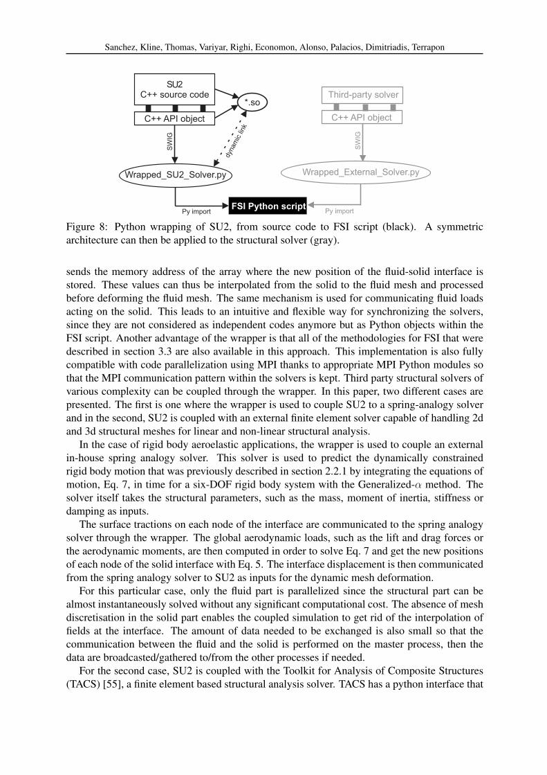
The flexibility of the Python language is used to couple SU2 with other third-party structuralsolvers in order to perform externally-coupled FSI simulations. Some specific functions imple-mented in SU2, such as those performing CFD iterations or mesh deformation, are rearrangedin a new C++/API object representing the SU2 solver as the fluid part of the FSI algorithm.The SU2 code with the API object are then compiled as a dynamic library using any C++ com-piler. An additional compilation using SWIG is required to translate the API into a wrappingPython module that is linked with the library and importable in any Python script where theFSI algorithm is built. In this way, the SU2 solver, through the Python-wrapped API, can bemanaged in an intuitive language but the critical and computationally intensive calculations areperformed with the same C++ routines as in the basic source code. This wrapping methodologyis illustrated in the left (black) part of Fig. 8.

3.4.2 Coupling with a third party solver

The coupling with external structural solvers is achieved within the Python script itself, pro-viding the considered solver also has a Python-translated API that can be imported as a Pythonmodule representing the solid part of the computation. This is illustrated in the right (gray) partof Fig. 8. For modularity purposes, the methods of the API object of any structural solver to becoupled with the Python wrapper should be built on a template that covers the main steps of anFSI algorithm.

The communications between the fluid and solid modules can be directly performed throughmemory by explicitly exchanging memory addresses as input/output to/from the specific APIfunctions. For example, when an update of the solid displacement is needed, the solid part


S 2C++ source code

U

C++ API object

Wrapped_SU2_Solver.py

*.so

SW

IG

dyn

am

ic li

nk

FSI Python scriptPy import

Third-party solver

C++ API object

Wrapped_External_Solver.py

SW

IG

Py import

Figure 8: Python wrapping of SU2, from source code to FSI script (black). A symmetricarchitecture can then be applied to the structural solver (gray).

sends the memory address of the array where the new position of the fluid-solid interface isstored. These values can thus be interpolated from the solid to the fluid mesh and processedbefore deforming the fluid mesh. The same mechanism is used for communicating fluid loadsacting on the solid. This leads to an intuitive and flexible way for synchronizing the solvers,since they are not considered as independent codes anymore but as Python objects within theFSI script. Another advantage of the wrapper is that all of the methodologies for FSI that weredescribed in section 3.3 are also available in this approach. This implementation is also fullycompatible with code parallelization using MPI thanks to appropriate MPI Python modules sothat the MPI communication pattern within the solvers is kept. Third party structural solvers ofvarious complexity can be coupled through the wrapper. In this paper, two different cases arepresented. The first is one where the wrapper is used to couple SU2 to a spring-analogy solverand in the second, SU2 is coupled with an external finite element solver capable of handling 2dand 3d structural meshes for linear and non-linear structural analysis.

In the case of rigid body aeroelastic applications, the wrapper is used to couple an externalin-house spring analogy solver. This solver is used to predict the dynamically constrainedrigid body motion that was previously described in section 2.2.1 by integrating the equations ofmotion, Eq. 7, in time for a six-DOF rigid body system with the Generalized-α method. Thesolver itself takes the structural parameters, such as the mass, moment of inertia, stiffness ordamping as inputs.

The surface tractions on each node of the interface are communicated to the spring analogysolver through the wrapper. The global aerodynamic loads, such as the lift and drag forces orthe aerodynamic moments, are then computed in order to solve Eq. 7 and get the new positionsof each node of the solid interface with Eq. 5. The interface displacement is then communicatedfrom the spring analogy solver to SU2 as inputs for the dynamic mesh deformation.

For this particular case, only the fluid part is parallelized since the structural part can bealmost instantaneously solved without any significant computational cost. The absence of meshdiscretisation in the solid part enables the coupled simulation to get rid of the interpolation offields at the interface. The amount of data needed to be exchanged is also small so that thecommunication between the fluid and the solid is performed on the master process, then thedata are broadcasted/gathered to/from the other processes if needed.

For the second case, SU2 is coupled with the Toolkit for Analysis of Composite Structures(TACS) [55], a finite element based structural analysis solver. TACS has a python interface that


allows it to be coupled easily with SU2. The load transfer between the fluid and structure solversis performed using an in-house python module developed for finite element based structuralweight estimation for aircraft configurations [56]. The python based FSI framework comprisingSU2, TACS and the load transfer module permits the solution of different FSI problems (steadyand unsteady) in two and three dimensions. Different fluid structure coupling architectures likethe Conventional Staggered or Block Gauss Seidel can be formulated without recompiling SU2or TACS simply by rearranging the function calls to the fluid and structural modules in thePython driver scripts. A test case for the unsteady solution of an elastic beam behind a squarecylinder (shown in in Section 4.2.3) is used to demonstrate the capabilities of the framework.

4 RESULTS

4.1 Fluid-Structure Interaction solver for rigid body applications

A typical aeroelastic reference model is the two-dimensional pitching-plunging airfoil [57](2 DOF) with a chord c in a free-stream flow of velocity U∞ (or Mach number M∞). Thismodel is illustrated in Fig. 9. The displacement h of the elastic axis is positive downwards andthe pitch angle α is positive clockwise. The positions along the chord of the center of gravityxCG and the elastic axis xf are considered from the nose of the airfoil. The product betweenthe distance (xCG − xf) and the airfoil mass m is the static unbalance S. The spring analogycontrols the motion of the airfoil with a stiffness Kh (or Kα) and a damping Ch (or Cα) for theplunging (or pitching) mode.

xfxCG cc/2

h t( )

α t( )

Kh

Kα

Cα

Ch

CG

U

x

y

Figure 9: Schematic of a two degrees of freedom pitching-plunging airfoil aeroelastic model.

The equations of motion, Eq. 7, for this aeroelastic system can be written as:

mh+ Sα + Chh+Khh = −LSh+ If α + Cαα +Kαα = M

(17)

where If is the inertia of the airfoil around the elastic axis, L the lift and M the aerodynamicmoment around the elastic axis. The lift is positive upwards and the aerodynamic momentaround the elastic axis is considered positive clockwise, as the pitch angle. This model can alsobe described by a set of non-dimensional parameters, i.e., the normalized static unbalance χand inertia rα, the uncoupled natural frequency ratio ω and the mass ratio µ:

χ =S

mb, rα =

If

mb2, ω =

ωhωα

, µ =m

πρ∞b2(18)


In these expressions b is the half-chord, ωh =√Kh/m (ωα =

√Kα/If) is the uncoupled

plunging (pitching) natural frequency and ρ∞ is the free-stream density of the fluid.

4.1.1 Two-dimensional pitching-plunging NACA 0012 airfoil

The Python wrapper is used here to couple SU2 with the basic spring analogy integratordescribed in section 3.4.2 to solve the basic two-dimensional aeroelastic problem involving apitching-plunging NACA 0012 airfoil in a free-stream flow. The unsteady RANS solver of SU2is used with the k − ω SST turbulence model and the FSI simulation is based on a strongly-coupled scheme with a tolerance on the solid displacement of 10−6 (leading to about 4 FSIiterations).

The case is set with the non-dimensional parameters χ = 0.25, rα = 0.5, ω = 0.3185and µ = 100. The elastic axis is placed at the quarter-chord point. Several free-stream Machnumbers are considered in order to capture both sub- and post-critical conditions. The chord-based Reynolds number is fixed at a value Rec = 4 · 106 for a chord c = 1 m. The naturalpitching frequency is set to ωα = 45 rad/s. A pitch angle for the airfoil of α = 0.872 rad (5o)is used as initial condition. These parameters are chosen in order to predict a subsonic flutterMach number that allows the comparison with incompressible theoretical models (see below).The calculations are performed with 139 time steps per period of the pitch mode for accuracypurposes.

The sub-critical response of the system for M∞ = 0.1 is compared with theoretical pre-dictions using the thin airfoil theory [58] for aerodynamic load predictions and Wagner func-tion [59] for dynamic fluid-solid coupling. Fig. 10 shows the normalized plunge displacementand pitch angle as a function of a non-dimensional time τ = ωαt. At this sub-critical Machnumber the system is strongly damped. The coupled computation is in good agreement with thetheoretical expectations, particularly for the pitch mode.

0 20 40 60 80 100 120

τ

-0.04

-0.02

0

0.02

0.04

h/b

Wagner model

Coupled computation

(a) Plunge displacement

0 20 40 60 80 100 120

τ

-0.1

-0.05

0

0.05

0.1

α[rad]

(b) Pitch angle

Figure 10: Aeroelastic response as a function of time at sub-critical conditions (M∞ = 0.1).

The Python wrapper is thus able to capture the response at flow conditions being quite farfrom critical conditions (flutter). Fig. 11 shows the computed responses of the plunging and


pitching modes at three different free-stream Mach numbers corresponding to sub-critical, crit-ical and post-critical conditions. The flutter Mach number, M∞ = 0.357, obtained from thecomputation differs only slightly from the theoretical prediction based on Wagner model, i.e.,M th∞ = 0.371. As expected, the response at M∞ = 0.3 is strongly damped. An increase of

the Mach number reduces the damping ratio until critical conditions are reached, at which theamplitude of the response remains constant in time. Finally, at post-critical conditions (e.g.,M∞ = 0.364), the response becomes unstable.

0 10 20 30 40 50 60 70

τ

-0.4

-0.2

0

0.2

0.4

h/b

M∞

= 0.3

M∞

= 0.357

M∞

= 0.364

(a) Plunge displacement

0 10 20 30 40 50 60 70

τ

-0.3

-0.2

-0.1

0

0.1

0.2

0.3

α[rad]

(b) Pitch angle

Figure 11: Aeroelastic response as a function of time at sub- and post-critical conditions.

Fig. 12 shows the computed dimensionless frequencies of the two airfoil modes as a funcionof the free-stream Mach number. The evolution of the frequencies is in good agreement withthe theoretical model. In particular, the two frequencies converge with increasingM∞ until theycoincide at the flutter Mach number and beyond it.

At the post-critical conditions the amplitude of the response is strongly amplified duringthe first 6 cycles, but then reaches a limit-cycle oscillation (LCO). This is due to the nonlineareffects of boundary layer separation and stall that appear for large displacements and anglesof attack. Fig. 13 shows the temporal response of the system over a longer time period. Thered bullets correspond to instants when significant flow separation occurs alternatively on theextrados or intrados of the airfoil. A sudden drop of the amplitude is systematically observedafter each separation. Subsequently, the amplitude increases again due to flutter instabilitiesbefore reaching another separation point. This mechanism allows the aeroelastic response toremain bounded in time and explains the development of a LCO mode.

A visualization of this flow dynamics is shown in Fig. 14 for times corresponding to thesecond set of red bullets in Fig. 13. The separation occurs when the two airfoil modes reachtheir local maximum values. On the suction side, the local Mach number becomes very large(close to 1.6) [Fig. 13 (a) and (b)]. Then a massive flow separation event is observed while theairfoil moves back towards its neutral position (α = h = 0) [Fig. 13 (c) and (d)]. Finally, theflow progressively reattaches until the instantaneous displacement (both modes) of the airfoil isclose to zero [Fig. 13 (e) and (f)]. A similar dynamics takes place for negative pitching angles.This highlights the capabilities of the wrapper coupling method to predict complex and non-linear dynamics that can be observed in aeroelastic systems beyond the linear coupled mode


0 0.05 0.1 0.15 0.2 0.25 0.3 0.35 0.4 0.45

M∞

0

0.2

0.4

0.6

0.8

1

1.2

ω/ωα

Flutter point

Plunge mode Wagner

Pitch mode Wagner

Plunge mode computed

Pitch mode computed

Figure 12: Dimensionless frequencies of the aeroelastic response as a function of the free-stream Mach number.

0 50 100 150 200 250

τ

-0.5

0

0.5

h/b,

α[rad]

plunge mode

pitch mode

Figure 13: LCO response of the system at M∞ = 0.364 under non-linear aerodynamic phe-nomena. The times when massive boundary layer separation occurs are marked by the redbullets.

flutter, keeping in mind the loss of accuracy for separated flows due to the RANS model.

4.1.2 Isogai wing section

The Python wrapper coupling SU2 and the spring-analogy integrator is also applied to theclassical Isogai wing section aeroelastic case (case A) [60,61]. This test case represents the dy-namics of the outboard portion of a swept back wing in the transonic regime. The correspondingparameters are χ = 1.8, rα = 1.865, ω = 1, µ = 60. The elastic axis is placed in front of theairfoil at a distance xf = −b from the leading edge and the natural pitching frequency is here


τ = 85.95 τ = 86.40 τ = 86.85

τ = 87.30 τ = 87.75 τ = 88.20

(a) (b) (c)

(e)(d) (f)

Figure 14: Visualization of the flow separation mechanism leading to a LCO response of thesystem beyond the flutter point.

set to ωα = 100 rad/s.The Euler equations are considered in the transonic regime (M∞ = 0.7− 0.9) with an initial

pitch angle for the airfoil of α0 = 0.0174 rad (1o) and the FSI simulation is again performedwith a strong-coupling scheme with the same tolerance than the previous test case. For thiscase, the number of time steps per period of the pitch mode is reduced to 39.

Several FSI simulations at different transonic Mach numbers are performed with variablespeed index

V ∗ =U∞

bωα√µ

(19)

in order to predict the flutter point. This state is reached when the damping extracted fromthe dynamic response of the system is close to zero. The results are illustrated in Fig. 15 thatshows a comparison of the computed flutter speed indices with those found in other references[62–65]. The best approximation curve (spline) is a representation of the limit between stableand unstable regions. It can be seen that the ”transonic dip” and the typical ”S-shape” flutterboundary for M∞ between 0.7 and 0.9 are both well predicted.

4.1.3 Test cases from the 2nd AIAA Aeroelastic Prediction Workshop

The second AIAA Aeroelastic Prediction Workshop [66] was officially launched in January2015 and took place in January 2016 (both events at Scitech) with the aim of assessing theaccuracy of the predictions provided by the available numerical approaches. The planned testcases include the investigation of forced and unforced wing oscillations as well as the studyof wing flutter with a pitch-and-plunge kinematics. All measurements were carried out by


0.7 0.75 0.8 0.85 0.9 0.95

M∞

0

0.5

1

1.5

2

2.5

3

V∗ f

Stable

Unstable

Current calculations

Spline interpolation

Liu et al.

Alonso & Jameson

Biao et al.

Thomas et al.

Figure 15: Flutter speed index as a function of the free-stream Mach number. Comparisonbetween current computations and numerical results from the literature.

NASA in Langley’s TDT wind tunnel. The wing model is the Benchmark Supercritical Wing(BSCW) [67–69]. All test cases are transonic and supercritical for the BSCW wing. Machnumber ranges between 0.70 and 0.84, Reynolds number (based on chord) is around 5 million.The fluids used for the experiments are heavy gases (R12 and R134a depending on the testcase). The angle of attack is chosen in order to position the shock wave differently in each testcase. The boundary layer is tripped at 7% of the chord. The three dimensionality of the flow inthe tip region – the BSCW wing has an aspect ratio of 4 – contributes to the complexity of thecase.

Pre-requisites for a physically consistent simulation include the full resolution of the bound-ary layer, and an acceptable prediction of the steady-state shock-boundary layer interaction,hence a correct positioning of the shock on the upper and lower side of the wing.

The fluid solver in SU2 has been used to simulate test case 1, which includes forced pitch os-cillations around the axis at 30% of the chord at frequency 10 Hz with an amplitude of±1. Themedian angle of attack of 3 is sufficient to generate a small supersonic region around the upperside of the nose of the wing and a shock at approximately 10% of the chord. The distributionof the pressure, obtained from SU2, is shown in Fig. 16. A time-accurate simulation with rigidgrid motion was conducted with the second order dual-time stepping, following a steady-statesolution, also obtained with SU2. Both simulations were run with the central scheme (JST). TheSpalart-Allmaras one-equation turbulence model [13] was used. For the steady-state simulationand for the subiterations in the time-accurate run, a CFL of 4.0 was used with the Euler implicittime stepping (iterations limited to 5).

Time-accurate pressure measurements - static data and first harmonic - are available in anumber of points at the section at 60% of the span. The results obtained with SU2 are comparedwith experimental data, whenever available, and with those obtained with Edge [70], a well-known CFD package developed by the Swedish Defence Research Centre (FOI) for aeroelastic


problems.

Figure 16: Steady state solution, pressure coefficient distribution over upper and lower wingsides

x/c

0 0.2 0.4 0.6 0.8 1

Cp

-1

-0.5

0

0.5

1

SU2

Edge

Exp

Figure 17: Pressure coefficient distribution averaged over ten periods

The agreement with the experimental data in terms of average pressure coefficient, presentedin Fig. 16, may be considered as good despite a difference of a few percentage points of chordin shock position. The agreement between SU2 and Edge is excellent. The comparison of thefirst harmonic (10 Hz), which is presented in Fig. 18 (magnitude of oscillations) and Fig. 19(phase delay with respect to pitch signal) shows again a very good agreement between SU2and Edge and larger deviations, but still acceptable to engineering standards, between CFDand experiments. The most noticeable differences concern the recovery area, downstream of


x/c

0 0.2 0.4 0.6 0.8 1

Cp

0.05

0.1

0.15

0.2

0.25

0.3

0.35

0.4

SU2

Edge

Exp

x/c

0 0.1 0.2 0.3 0.4 0.5 0.6 0.7 0.8 0.9 1

Cp

0.02

0.04

0.06

0.08

0.1

0.12SU2

Edge

Exp

Figure 18: First harmonic of response, magnitude, pressure coefficient, upper (lhs) and lower(rhs) wing side

x/c

0 0.2 0.4 0.6 0.8 1

DE

G

-100

-50

0

50

100SU2

Edge

Exp

x/c

0 0.2 0.4 0.6 0.8 1

DE

G

0

20

40

60

80

100

120

140

160

180SU2

Edge

Exp

Figure 19: First harmonic of response, phase delay in degrees, pressure coefficient, upper (lhs)and lower (rhs) wing side

the shock, where the predicted phase angle is overestimated, and the shock area, where theexperimental data show much lower value in correspondence of sensor 5. The most likely cause- according to the researchers and organizers of the Workshop - is some local deformationeffect which is not being taken into consideration in CFD simulation. Two effects are expectedto play a major role in the evolution of static pressure on the upper wing side as a function ofthe oscillating pitch angle; on the one hand, the motion of the stagnation point causes a firstpressure peak to grow in phase with pitch angle, on the other hand, the shock wave moves upand downstream also in phase with the pitch angle. The two effects generate a “double peak”,which is clearly visible in Fig. 18, in both CFD and experimental data.

The flow being strongly non-linear, the response of the aerodynamics contains several non-negligible harmonics; the Fourier expansion of the pressure coefficients has a non negligibleamplitude at the reference frequency f = 10Hz and also at 2× f , 3× f and 4× f . This is pre-sented in Fig. 20. Again, the agreement between SU2 and Edge is very good. No experimentaldata is available for frequencies higher than 10 Hz.


x/c

0 0.2 0.4 0.6 0.8 1

Cp

0.02

0.04

0.06

0.08

0.1

0.12

0.14

SU2

Edge

x/c

0 0.2 0.4 0.6 0.8 1

Cp

0.01

0.02

0.03

0.04

0.05

0.06

0.07

0.08 SU2

Edge

x/c

0 0.2 0.4 0.6 0.8 1

Cp

0.01

0.02

0.03

0.04

0.05

0.06

SU2

Edge

Figure 20: Second, third and fourth harmonics of response, magnitude, pressure coefficient

4.2 Fluid-Structure Interaction solver with deformable solids

4.2.1 Benchmark problem for native FSI solver in SU2

In order to test our native implementation of the FSI solver for deformable solids within SU2,we focus on a well-known benchmark test case first proposed by Wall and Ramm [71] (see, forexample, [35, 44, 72–75]). They investigated the dynamics of a flexible cantilever attached tothe downwind side of a square cylinder in a low-speed flow, as described in Fig. 21.

14 .5 H

12 H

H L

tH

5 H

u

x

y

slip-wall

outlet

8

H L

Geometry:==

t =

14

0.06

uρ

Fluid properties==

μ =

0.5131.18

∞

f

f

cm

m/skg/mkg/m s

cmcm

1.82 10. -5

3

.

Eρ

Structural properties==

ν =100s

Pakg/m

0.35

3

.2.50 10 5

Re = 332

slip-wall

Figure 21: Benchmark for FSI solver with deformable solids.

The physics that lie behind this problem may be briefly described as follows. The squarecylinder, rigid and static, generates vortical structures in the low-Reynolds number flow. Thesevortices generate an alternating pressure in the wake, that induces motions of the flexible can-tilever attached to the downwind side of the square, as shown in Fig. 22.

Figure 22: Pressure contours and structural displacements for the benchmark test cases for afull cycle of oscillation. From left to right, T=0, T=π/2, T= π, T=3π/2.


The two parameters that have been used in the literature to assess the validity of differentFSI implementations are the frequency and amplitude of the vertical displacement at the tip ofthe cantilever. With regards to the frequency, published values range from 2.78 to 3.25 Hz, thisis, in the surroundings of the first natural frequency of the cantilever, equal to 3.03 Hz. Themaximum tip displacement has been found to be within the range 1-1.4 cm, thus a 25-35% ofthe cantilever length, which results in geometrically-nonlinear effects on the structure.

We have tested this problem using SU2 and several different time and space discretisations.In these tests, we have obtained values of frequency ranging from 3.05 to 3.15 Hz and maximumtip displacements in the range of 1.05 - 1.15 cm, showing a very good agreement with the liter-ature. In a previous work, see [7], we have also shown the ability of the solver to capture somemodulations in the amplitude due to the complex physics involved, and the different behaviourof the coupled problem when modifying some relevant parameters, such as the structural densityand first natural frequency.

In order to reduce the computational time, we have also tested in this work the ability of theAitken’s dynamic parameter and the first order displacement predictor to reduce the number ofBGS subiterations. In Fig. 23, we compare different configurations against a BGS strongly-coupled strategy in which we use a fixed relaxation parameter ωfixed = 0.5. This approachconverges slowly to the solution, in about 8-10 iterations per time step.

5 6 7 8 9 101.5

1.0

0.5

0.0

0.5

1.0

1.5

5 6 7 8 9 101.5

1.0

0.5

0.0

0.5

1.0

1.5

5 6 7 8 9 101.5

1.0

0.5

0.0

0.5

1.0

1.5

5 6 7 8 9 101.5

1.0

0.5

0.0

0.5

1.0

1.5

5 6 7 8 9 10

Time (s)

0

2

4

6

8

10

12

5 6 7 8 9 10

Time (s)

0

2

4

6

8

10

12

5 6 7 8 9 10

Time (s)

0

2

4

6

8

10

12

5 6 7 8 9 10

Time (s)

0

2

4

6

8

10

12

Dis

plac

emen

t (cm

)

ωfixed=0 7 ωfixed=0 9 ωAitken dyn ωAitken dyn + Predictor

Num

ber

of it

erat

ions

. . , ,

Figure 23: Time histories of the vertical tip displacements for different values of the relaxationparameter for the BGS FSI solver. The base solution (in grey) is obtained with ωfixed = 0.5, andno predictor.

By increasing the fixed relaxation parameter to ωfixed = 0.7, we reduce the computationaltime in a 33%. However, as it may be seen in Figure 23, a higher relaxation parameter introducessome deviations in the solution, that we believe are closely related to the value of ω being toolarge in the first subiteration, ω0. This effect becomes more clear when we increase the fixedrelaxation parameter to ωfixed = 0.9, when both the frequency and the amplitude are affected


and the amplitude modulation is almost damped out.On the other hand, the use of the Aitken’s dynamic relaxation parameter (ωAitken,dyn) clearly

improves the convergence of the scheme. In particular, the number of BGS subiterations isreduced to 4-5 per time step, resulting in the computational time being a 38% shorter. Byusing a first order predictor on the first BGS subiteration, we can further reduce the number ofiterations to 3-4 and the computational time by a 56% with respect to the baseline case, whileobtaining effectively the same solution. It is important to note that, in these two cases, we havelimited the value of the relaxation parameter in the first BGS iteration to ω0 = 0.5, then allowingit to adapt dynamically in the remaining subiterations.

4.2.2 Interpolation framework for non-matching discretizations

To test the implementation of the interpolation routines, the case of a solid wall immersed ina flow in a channel case is used. The geometry is shown in Fig. 24, and the flow conditions wereset as Mach 0.15 viscous unsteady flow with adiabatic no-slip walls on the flexible vertical wallwithin the channel, and slip wall conditions on the upper and lower surfaces. The Reynoldsnumber is 300 per meter. The ratio of densities between the structure and the fluid is 1 : 0.0106.

t

h

L

Hinlet

upper

lower

outlet

L = 0.20 m

H = 0.02 m

t = 0.001 m

h = 0.016 m

x

y

wall

Figure 24: Test case used for interpolation routines.

Several meshes were generated with varying refinement. The results shown are from a ’fine’mesh with 100 elements on the upwind surface of the vertical wall, and a ’coarser’ mesh with90 elements on that same wall. Fig. 25 illustrates the results of simulating the coupled dy-namics with either matching ’fine’ discretizations, matching ’coarser’ discretizations, or a non-matching discretization with the ’coarser’ mesh used for the structural dynamics. This plot il-lustrates the effect of using these methods on the accuracy of the solution. Figure 26 illustratesthe deformed geometry at time step 25. We can see from these plots that the nearest-neighborinterpolation results in discontinuous values. Using isoparametric weighting coefficients resultsin a smoother deformation, however when examining the accuracy of this deformation in Fig-ure 25, we can see that a smoother interpolation has not resulted in more accurate results ascompared to the nearest neighbor approach. Both of these methods use a transformation ma-trix H that has been calculated separately for the two transfer directions. The combination ofthis smoother interpolation and the use of a single H results in the most accurate interpolatedresults.

4.2.3 Python-wrapped FSI with interface to external solvers

In order to test/demonstrate the flexibility of the python interface of SU2, the FSI problemof a flexible cantilever attached to the downwind side of a square cylinder (described in Section4.2.1) is solved by coupling the flow and structural solvers using the python interface. The


Figure 25: Time history of horizontal displacement of the upper right-hand corner of the de-flecting beam. The geometry has been held static until time step 18.

(a) Matching discretiza-tion.

(b) Unmatched dis-cretization with Nearest-Neighbor interpolation.Discontinuities can beseen in the deformedshape.

(c) Unmatched discretiza-tion with Isoparametricweights used in interpo-lation. The deformationis smooth, but does notagree with matched dis-cretization results.

(d) Unmatched dis-cretization with ’Con-servative’ method as inSection 2.3.3. The defor-mation agrees with thematched discretization,and is smooth.

Figure 26: Deformed geometry after 25 time steps

geometry of the problem is the same as Section 4.2.1 but the conditions are slightly differentcorresponding to those specified in Dettmer et al. [73]. These are stated again in Fig. 27. Theresults shown in Figs. 28, 29 were computed using a conventional staggered (CS) couplingapproach. We see that the maximum tip displacement of the beam, not including the transientregion, is 1.03 and the average frequency is 2.93 Hz showing a good agreement with [73] andthe results in Section 4.2.1. Simulations with the Block Gauss Seidel (BGS) coupling approachgive similar results but these have not been shown here.


Figure 27: Geometry, flow and structural properties used for the 2d simulation using the pythoninterface

Figure 28: Time history of vertical tip displacements obtained using the python based coupling

Figure 29: Convective flux contours and structural displacements for the benchmark test cases(using the python based framework) for a full cycle of oscillation. From left to right, T=0,T=π/2, T= π, T=3π/2.

5 CONCLUSION

We have introduced a new open-source Fluid-Structure Interaction solution framework tai-lored to high-fidelity analysis in computational aeroelasticity. It includes a natively embeddedFSI solver and a code wrapper methodology that simplify the communication of the code withother external commercial and in-house solvers. We have carried out some relevant tests of themethodology and the different capabilities that have been implemented. We have compared theresults obtained using this software with some relevant benchmark test cases, obtaining resultsthat agree well with the open literature.

This infrastructure has been implemented by an international group of researchers with dif-ferent backgrounds and expertise, and is publicly available in a github repository that can beaccessed through the SU2 project website, http://su2.stanford.edu/. The main goal of this col-laborative work is to progressively incorporate new capabilities into the platform while main-taining its modularity, thus encouraging for further developments of state-of-the-art techniques


within the different disciplines that conform the study of the interaction between fluids andstructures.

ACKNOWLEDGEMENTS

H. Kline would like to acknowledge the support of a NASA Space Technology ResearchFellowship.

REFERENCES

[1] C. Farhat, M. Lesoinne, and P. LeTallec. Load and motion transfer algorithms forfluid/structure interaction problems with non-matching discrete interfaces: Momentumand energy conservation, optimal discretization and application to aeroelasticity. Com-puter Methods in Applied Mechanics and Engineering, 157(1-2):95–114, 1998.

[2] A. Beckert. Coupling fluid (CFD) and structural (FE) models using finite interpolationelements. Aerospace Science and Technology, 4(1):13–22, 2000.

[3] C. Farhat, K.G. van der Zee, and P. Geuzaine. Provably second-order time-accurateloosely-coupled solution algorithms for transient nonlinear computational aeroelasticity.Computer Methods in Applied Mechanics and Engineering, 195(17-18):1973–2001, 2006.

[4] F. Palacios, M.R. Colonno, A.C. Aranake, A. Campos, S.R. Copeland, T.D. Economon,A.K. Lonkar, T.W. Lukaczyk, T.W.R. Taylor, and J.J. Alonso. Stanford UniversityUnstructured (SU2): An open-source integrated computational environment for multi-physics simulation and design. In AIAA 51st Aerospace Sciences Meeting, 7-10 January,Grapevine, TX, 2013.

[5] F. Palacios, T.D. Economon, A.C. Aranake, S.R. Copeland, A.K. Lonkar, T.W. Lukaczyk,D.E. Manosalvas, K.R. Naik, A. Santiago Padrn, B. Tracey, A. Variyar, and J.J. Alonso.Stanford university unstructured (SU2): Open-source analysis and design technology forturbulent flows. In AIAA 52nd Aerospace Sciences Meeting, SciTech, 13-17 January, Na-tional Harbor, MD, 2014.

[6] T. Economon, F. Palacios, J. Alonso, G. Bansal, D. Mudigere, A. Deshpande, A. Hei-necke, and A. Smelyanskiy. Towards High-Performance Optimizations of the Unstruc-tured Open-Source SU2 suite. In AIAA 53rd Aerospace Sciences Meeting, Scitech, 5-9January, Kissimmee , FL, 2015.

[7] R. Sanchez, R. Palacios, T.D. Economon, H.L. Kline, J.J. Alonso, and F. Palacios. Towardsa Fluid-Structure Interaction solver for problems with large deformations within the open-source SU2 suite. In 57th AIAA/ASCE/AHS/ASC Structures, Structural Dynamics, andMaterials Conference, AIAA SciTech, 4-8 Jan, 2016.

[8] J. Donea, A. Huerta, J.-Ph. Ponthot, and A. Rodriguez-Ferran. Arbitrary Lagrangian-Eulerian Methods in Encyclopedia of Computational Mechanics. John Wiley and Sons,2004.

[9] C. Hirsch. Numerical Computation of Internal and External Flows. Wiley, New York,1984.


[10] D.C. Wilcox. Turbulence Modeling for CFD. 2nd Ed., DCW Industries, Inc., 1998.

[11] F. M. White. Viscous Fluid Flow. McGraw Hill Inc., New York, 1974.

[12] F.R. Menter. Zonal two equation k − ω, turbulence models for aerodynamic flows. AIAAPaper 1993-2906, 1993.

[13] P. Spalart and S. Allmaras. A one-equation turbulence model for aerodynamic flows.Number AIAA Paper 1992-0439, 1992.

[14] A. Jameson, W. Schmidt, and E. Turkel. Numerical solution of the Euler equations byfinite volume methods using Runge-Kutta time stepping schemes. Number AIAA Paper1981-1259, 1981.

[15] P. L. Roe. Approximate riemann solvers, parameter vectors, and difference schemes.Journal of Computational Physics, 43(2):357 – 372, 1981.

[16] J. M. Weiss, J. P. Maruszewski, and A. S. Wayne. Implicit solution of the Navier-Stokesequation on unstructured meshes. AIAA Paper 1997-2103, 1997.

[17] A. Jameson. Time dependent calculations using multigrid, with applications to unsteadyflows past airfoils and wings. Number AIAA Paper 1991-1596, 1991.

[18] A. Jameson and S. Schenectady. An assessment of dual-time stepping, time spectral andartificial compressibility based numerical algorithms for unsteady flow with applicationsto flapping wings. Number AIAA Paper 2009-4273, 2009.

[19] P. D. Thomas and C. K. Lombard. Geometric conservation law and its application to flowcomputations on moving grids. AIAA Journal, 17(10):1030–1037, October 1979.

[20] J. T. Batina. Unsteady Euler airfoil solutions using unstructured dynamic meshes. AIAAJournal, 28(8):1381–1388, August 1990.

[21] M. Lesoinne and C. Farhat. Geometric conservation laws for flow problems with movingboundaries and deformable meshes, and their impact on aeroelastic computations. Com-puter Methods in Applied Mechanics and Engineering, 134(1–2):71 – 90, 1996.

[22] C. Farhat, P. Geuzaine, and C. Grandmont. The discrete geometric conservation law andthe nonlinear stability of ALE schemes for the solution of flow problems. Journal ofComputational Physics, 174(2):669–694, December 2001.

[23] S. A. Morton, R. B. Melville, and M. R. Visbal. Accuracy and coupling issues of aeroe-lastic Navier-Stokes solutions on deforming meshes. Journal of Aircraft, 35(5):798–805,1998.

[24] R. T. Biedron and J. L. Thomas. Recent enhancements to the FUN3D flow solver formoving-mesh applications. AIAA Paper 2009-1360, 2009.

[25] M. Geradin and A. Cardnna. Flexible Multibody Dynamics, A Finite Element Approach,chapter Kinematics of Finite Motion. John Wiley & Sons, LTD, 2001.

[26] M. Geradin and D.J. Rixen. Mechanical Vibrations : Theory and Application to StructuralDynamics, chapter Analytical Dynamics of Discrete Systems. Wiley, 2015.


[27] F. Amirouche. Fundamentals of Multibody Dynamics, Theory and Applications, chapterHamilton-Lagrange and Gibbs-Appel Equations. Birkhauser, 2006.

[28] M. Hojjat, E. Stavropoulou, T. Gallinger, U. Israel, R. Wchner, and Bletzinger K.-U. FluidStructure Interaction II, volume 73, chapter Fluid-Structure Interaction in the Contextof Shape Optimization and Computational Wind Engineering, pages 351–381. SpringerBerlin Heidelberg, 2010.

[29] J. Bonet and R. D. Wood. Nonlinear Continuum Mechanics for Finite Element Analysis.Cambridge University Press, 1997.

[30] J. Donea, A. Huerta, J.-Ph. Ponthot, and A. Rodrıguez-Ferran. Encyclopedia of Computa-tional Mechanics, chapter Arbitrary Lagrangian-Eulerian Methods. John Wiley & Sons,Ltd, 2004.

[31] K.-J. Bathe. Finite Element Procedures in Engineering Analysis. Civil engineering andengineering mechanics series. Prentice-Hall, 1982.

[32] N. M. Newmark. A method of computation for structural dynamics. Journal of the Engi-neering Mechanics Division, 85(3):67–94, 1959.

[33] J. Chung and G.M. Hulbert. Time integration algorithm for structural dynamics with im-proved numerical dissipation: the generalized-α method. Journal of Applied Mechanics,Transactions ASME, 60(2):371–375, 1993.

[34] S. Deparis, M. Discacciati, G. Fourestey, and A. Quarteroni. Fluid-structure algorithmsbased on Steklov-Poincare operators. Computer Methods in Applied Mechanics and En-gineering, 195(41-43):5797–5812, 2006.

[35] C. Kassiotis, A. Ibrahimbegovic, R. Niekamp, and H.G. Matthies. Nonlinear fluid-structure interaction problem. part I: Implicit partitioned algorithm, nonlinear stabilityproof and validation examples. Computational Mechanics, 47(3):305–323, 2011.

[36] S. Piperno and C. Farhat. Partitioned procedures for the transient solution of coupledaeroelastic problems part II: energy transfer analysis and three-dimensional applications.Computer Methods in Applied Mechanics and Engineering, 190(2425):3147–3170, 2001.Advances in Computational Methods for Fluid-Structure Interaction.

[37] C. Farhat, M. Lesoinne, P. Stern, and S. Lantri. High performance solution of three-dimensional nonlinear aeroelastic problems via parallel partitioned algorithms: Method-ology and preliminary results. Advances in Engineering Software, 28(1):43–61, 1997.

[38] C. Farhat and M. Lesoinne. Two efficient staggered algorithms for the serial and parallelsolution of three-dimensional nonlinear transient aeroelastic problems. Computer Methodsin Applied Mechanics and Engineering, 182(34):499–515, 2000.

[39] W.G. Dettmer and D. Peric. A new staggered scheme for fluid-structure interaction. In-ternational Journal for Numerical Methods in Engineering, 93(1):1–22, 2013.

[40] M. Von Scheven and E. Ramm. Strong coupling schemes for interaction of thin-walledstructures and incompressible flows. International Journal for Numerical Methods inEngineering, 87(1-5):214–231, 2011.


[41] J. Degroote, K.-J. Bathe, and J. Vierendeels. Performance of a new partitioned procedureversus a monolithic procedure in fluid-structure interaction. Computers and Structures,87(11-12):793–801, 2009.

[42] P. Le Tallec and J. Mouro. Fluid structure interaction with large structural displacements.Computer Methods in Applied Mechanics and Engineering, 190(24-25):3039–3067, 2001.

[43] U. Kuttler and W.A. Wall. Fixed-point fluid-structure interaction solvers with dynamicrelaxation. Computational Mechanics, 43(1):61–72, 2008.

[44] C. Habchi, S. Russeil, D. Bougeard, J.-L. Harion, T. Lemenand, A. Ghanem, D.D. Valle,and H. Peerhossaini. Partitioned solver for strongly coupled fluid-structure interaction.Computers and Fluids, 71:306–319, 2013.

[45] B. M. Irons and R. C. Tuck. A version of the Aitken accelerator for computer iteration.International Journal for Numerical Methods in Engineering, 1:275–277, 1969.

[46] M.J. Smith, D.H. Hodges, and C.E.S. Cesnik. Evaluation of computational algorithmssuitable for fluid-structure interactions. Journal of Aircraft, 37(2):282–294, 2000.

[47] J.R. Cebral and R. Lohner. Conservative load projection and tracking for fluid-structureproblems. AIAA Journal, 35(4):687–692, 1997.

[48] G.P. Guruswamy. A review of numerical fluids/structures interface methods for computa-tions using high-fidelity equations. Computers and Structures, 80(1):31–41, 2002.

[49] A. de Boer, A.H. van Zuijlen, and H. Bijl. Review of coupling methods for non-matchingmeshes. Computer Methods in Applied Mechanics and Engineering, 196(8):1515–1525,2007.

[50] X. Jiao and M.T. Heath. Overlaying surface meshes, part I: Algorithms. InternationalJournal of Computational Geometry and Applications, 14(6):379–402, 2004.

[51] R.K. Jaiman, X. Jiao, P.H. Geubelle, and E. Loth. Assessment of conservative load transferfor fluid-solid interface with non-matching meshes. International Journal for NumericalMethods in Engineering, 64(15):2014–2038, 2005.

[52] S A Brown. Displacement Extrapolations for CFD+CSM Aeroelastic Analysis. AIAAPaper, pages 291–300, 1997.

[53] A. Beckert and H. Wendland. Multivariate interpolation for fluid-structure-interactionproblems using radial basis functions. Aerospace Science and Technology, 5(2):125–134,2001.

[54] T. D. Economon, F. Palacios, S. R. Copeland, T. W. Lukaczyk, and J. J. Alonso. SU2: AnOpen-Source Suite for Multi-Physics Simulation and Design. AIAA Journal, (accepted),2015.

[55] G. J. Kennedy and J.R.R.A. Martins. A parallel aerostructural optimization framework foraircraft design studies. Structural and Multidisciplinary Optimization, Volume 50, Issue6, 2014.


[56] A. Variyar, T.D. Economon, and J. J. Alonso. Multifidelity conceptual design and opti-mization of strut-braced wing aircraft using physics based methods. 54th AIAA AerospaceSciences Meeting, 2016.

[57] R.L. Bisplinghoff, H. Ashley, and R. L. Halfman. Aeroelasticity. Dover Publications,1996.

[58] Anderson J.D. Fundamentals of Aerodynamics, chapter Incompressible Flow over Air-foils. Mc Graw Hill, Inc., 2011.

[59] Y. C. Fung. An Introduction to the theory of aeroelasticity, chapter Fundamentals of flutteranalysis. Dover Publications, 2002.

[60] K. Isogai. On the transonic-dip mechanism of flutter of a sweptback wing. AIAA Journal,17(7):793–795, 1979.

[61] K. Isogai. Transonic-dip mechanism of flutter of a sweptback wing: part ii. AIAA Journal,19(9):1240–1242, 1981.

[62] F. Liu, J. Cai, and Y. Zhu. Calculation of wing flutter by a coupled fluid-structure method.Journal of Aircraft, 38(2):334–342, 2001.

[63] J.J. Alonso and A. Jameson. Fully-implicit time marching aeroelastic solution. In AIAA32nd Aerospace Sciences Meeting and Exhibit, 10-13 January, 1994.

[64] Z. Biao, Q. Zhide, and G. Chao. Transonic flutter analysis of an airfoil with approximateboundary method. In 26th international congress of the aeronautical sciences, 2008.

[65] J.T. Thomas, K.C. Hall, and E.H. Dowell. Reduced-order aeroelastic modeling usingproper-orthogonal decomposition. CEAS/AIAA/ICASE/NASA Langley International Fo-rum on Aeroelasticity and Structural Dynamics, 1999.

[66] J. Heeg, P. Chwalowski, D. M. Schuster, D. Raveh, A. Jirasek, and M. Dalenbring. Plansand example results for the 2nd AIAA Aeroelastic Prediction Workshop. AIAA Paper,2015.

[67] B. E. Dansberry, M. H. Durham, R. M. Bennett, D. L. Turnock, E. A. Silva, and J. A.Rivera Jr. Physical properties of the benchmark models program supercritical wing, vol-ume 4457. Citeseer, 1993.

[68] D. J. Piatak and C. S. Cleckner. Oscillating turntable for the measurement of unsteadyaerodynamic phenomena. Journal of aircraft, 40(1):181–188, 2003.

[69] R. M. Bennett, C. V. Eckstrom, J. A Rivera Jr, B. E. Dansberry, M. G. Farmer, and M. H.Durham. The benchmark aeroelastic models program: Description and highlights of initialresults. 1991.

[70] P. Eliasson and P. Weinerfelt. Recent Applications of the Flow Solver Edge. Proceedingsof the 7th Asian CFD Conference, 2007.

[71] W.A. Wall and E. Ramm. Fluid-Structure interaction based upon a stabilized (ALE) finiteelement method. In E. Onate S.R. Idelsohn and E.N. Dvorkin (Eds.), editors, Computa-tional Mechanics. New Trends and Applications. CIMNE, Barcelona, Spain, 1998.


[72] H. G. Matthies and J. Steindorf. Partitioned strong coupling algorithms for fluidstructureinteraction. Computers & Structures, 81(811):805–812, 2003.

[73] W. Dettmer and D. Peric. A computational framework for fluid-structure interaction: Fi-nite element formulation and applications. Computer Methods in Applied Mechanics andEngineering, 195(41-43):5754–5779, 2006.

[74] C. Wood, A.J. Gil, O. Hassan, and J. Bonet. A partitioned coupling approach for dy-namic fluid-structure interaction with applications to biological membranes. InternationalJournal for Numerical Methods in Fluids, 57(5):555–581, 2008.

[75] B. Froehle and P.-O. Persson. A high-order discontinuous Galerkin method for fluid-structure interaction with efficient implicit-explicit time stepping. Journal of Computa-tional Physics, 272:97–104, 2014.

assessment of the fluid-structure interaction … · vii european congress on computational methods...

Documents