asset price fluctuation and price indices

103

Asset Price Fluctuation and Price Indices

Asset Price Fluctuationand Price Indices

Shigenori Shiratsuka

Research Division 1, Institute for Monetary and Economic Studies, Bank of Japan (E-mail: [email protected])

This paper is an updated version of Shiratsuka (1996) written in Japanese. The author isgrateful to Hiroshi Shibuya for his helpful comments on the earlier draft; to MichaelBryan, Ben Craig, William T. Gavin, Ed Green, and seminar participants at the FederalReserve Bank of Chicago, Cleveland, and St. Louis for their useful comments and discus-sions; and to Laura Kutianski for her assistance to make this paper more readable.Opinions expressed are those of the author and do not necessarily reflect those of theBank of Japan.

MONETARY AND ECONOMIC STUDIES/DECEMBER 1999

Since the late 1980s, the Japanese economy has experienced tremendous rise and fall of asset prices and large fluctuations of realeconomic activity, while the general price level has remained rela-tively stable. Such developments have raised the question of whethermonetary policy should target asset prices rather than conventionalprice indices. This paper focuses on how to make use of informationinherent with asset price fluctuations in the monetary policy judgment. To this end, it investigates the possibility of incorporatingasset price data into inflation measures by extending the conven-tional price index concept into a dynamic framework. The mainconclusion of this paper is as follows. Although the concept of suchextensions of the conventional price index is highly evaluated from atheoretical viewpoint, it is difficult for monetary policy makers toexpect it to be more than a supplementary indicator for monetarypolicy judgment. This is because (1) reliability of asset price statisticsis quite low, compared with the conventional price indices; and (2) asset price changes do not necessarily mean that the future pricechanges, because there are a lot of sources for asset price fluctuationbesides the private-sector expectation for inflation.

Key words: Asset price; Intertemporal cost of living index;Dynamic equilibrium price index; Monetary policy;Information variable

I. Introduction

Looking at Japan’s macroeconomic development since the late 1980s, the so-called“bubble era,” asset prices rose and declined tremendously, and business conditionsfluctuated remarkably, while consumer and wholesale prices remained relatively stable. Such developments raised questions of whether monetary policy should havetargeted asset prices rather than conventional price indices.1 In general, asset pricesreflect market participants’ expectations about the future, and market expectationsseem to have played an important role behind the scene of the bubble economy.Keeping this question in mind, I examine the possibility of constructing a reliableinflation measure that includes asset price information from the theoretical and practical viewpoints.2

As far as monetary policy tries to achieve the medium- to long-run sustainableprice stability, it is insufficient to monitor the fluctuation of the conventional priceindices that reflect only information on the current inflation.3 By contrast, assetprices provide monetary policy makers with useful information in the sense thatvividly reflects the private-sector expectation for inflation.4 Moreover, the dynamicextension of the conventional price index concept indicates that asset prices are adesirable proxy for the future inflation. Alchian and Klein (1973) first proposed anintertemporal cost of living index (ICLI) to trace the intertemporal changes in thecost of living that is required to achieve a given level of intertemporal utility. Then,Shibuya (1992) formulated the ICLI as a practical index formula and named it thedynamic equilibrium price index (DEPI).

However, given the importance of asset price information, it difficult for mone-tary policy makers to employ such inflation measures as one of the core indicators in monetary policy judgment. This is because such inflation measures are hardlyoperational, since they are too unreliable to be used in any formal assessment of theexpected future course of inflation. Therefore, monetary policy makers cannot expectasset prices to be more than supplementary indicators of inflation pressures.5

104 MONETARY AND ECONOMIC STUDIES/DECEMBER 1999

1. See, for example, Noguchi (1992), Suzuki (1995), and Okina (1993). Matsushita (1995), the former Governor ofthe Bank of Japan, stated the role of asset prices in conducting monetary policy as follows:

In pursuit of price stability, however, we believe that it is not appropriate to treat the stability of asset prices,such as those of land and stocks, on the same basis as general price stability, and to include it in the goal ofmonetary policy. As asset prices move in response to the private-sector expectations for economic growth, it isimpossible to establish any clear criteria, such as that zero inflation is desirable as in the case of general prices.

2. When we consider the problems concerning the relationship between asset prices and monetary policy, the creditchannel is emphasized in the transmission mechanism that the fluctuation of asset prices affects real economicactivity. In addition, it is also an important point of discussion that financial crisis often occurs as an aftermath ofsignificant drops in asset prices. For the issues such as the relationship between asset price fluctuation and creditconstraint, and the impact on financial system stability, see, for example, Hoshi (1996), who surveys the recentresearches on these issues.

3. See Shiratsuka (1997) for the discussion on the practical definition of price stability as an objective of monetary policy.4. For the discussion on the role of asset prices as an information variable for monetary policy judgment, see Borio et

al. (1994). In addition, in relation to the argument in Bernanke and Woodford (1997), it should be noted that itis not the case that monetary policy makers can respond mechanically to private-sector inflation forecasts, sincesuch a policy response leads to indeterminacy of rational expectation equilibria. However, this paper concludesthat asset price information, while containing useful information on the future course of inflation and othermacroeconomic fluctuations, is too inaccurate to be adopted by monetary policy makers as a policy target variable.

5. Goodhart (1995) and his discussants (Bockelmann [1995] and Bruni [1995]) raise a similar argument on the feasibility of constructing a reliable inflation measure by combining the current price index and asset prices.

In this context, the following two points are crucial: (1) policy implication of assetprice fluctuation differs in accordance with the sources of asset price changes; and (2) acceptability of remarkably high weight for asset prices, suggested from the theoretical foundation, is questionable. More precisely, it is very difficult to interpretasset price information as a monetary policy indicator due to the possibility of elements in asset prices that reflect bubbles in the private-sector expectations and/orstructural changes in the economy. In addition, reliability of the current price indicesis by far higher than that for asset prices. While the current price indices are alsoaffected by measurement errors, their reliability is far higher than asset pricestatistics.6 Therefore, it seems quite difficult to construct a reliable price index thatincludes asset price information.

The rest of the paper is constructed as follows. In Chapter II, I discuss the possi-bility of incorporating asset price information into an inflation measure by extendingthe static price index concept into a dynamic framework. Then, I compute the DEPIand empirically examine the role of asset prices as an information variable for mone-tary policy in Chapter III. In Chapter IV, I explore the difficulties monetary policymakers will be faced with, if such a dynamic inflation measure that reflects the assetprice fluctuations as well as the current inflation is employed as the core indicator formonetary policy judgment. In Chapter V, I discuss the optimal inflation measure formonetary policy makers. Finally, in Chapter VI, I summarize the major results of thispaper, and conclude it. In the appendices, I explain the theoretical foundation of thedynamic price index concept, and estimate the observation errors in the consumerprice index (CPI), with its disaggregated data.

II. Extension of Price Index to Dynamic Framework

In this chapter, I explore the possibility of constructing a price index that incorpo-rates asset price data from the theoretical viewpoints. Then, I extend the con-ventional price index concept into the dynamic framework by taking into accountthe intertemporal optimization of consumer behavior.

A. Intertemporal Cost of Living IndexWhen we discuss price indices as a measure of change in cost of living, we alwaysfocus on the current consumption activity, and consider price indices as measures for tracing price changes from the base period up to the current period.7 However,consumer behavior possesses a dynamic nature so that current consumption dependsclosely on the future path of consumption. Moreover, since monetary policy tries toachieve the medium- to long-run sustainable price stability, it is insufficient to moni-tor the fluctuation of the conventional price indices that reflect only information onthe current inflation. Therefore, it would be reasonable to extend the conventional

105


6. Although it is true that the current price indices are also affected by measurement errors, their reliability is farhigher than asset price statistics. For the discussion on the measurement errors in the Japanese CPI, see Shiratsuka(1998, 1999).

7. For the details of theoretical foundation of price indices, see, for example, Shiratsuka (1998, 1999) and Pollak (1989).

price index concept into the dynamic framework so as to trace intertemporal changesin the cost of living.

Alchian and Klein (1973) proposed the idea of the intertemporal cost of livingindex (ICLI) that traces the intertemporal changes in the cost of living that arerequired to achieve a given level of intertemporal utility.8 In this case, since priceinformation for future goods and services is not readily available from futures markets, an alternative measure to extract such information must be devised.Considering the intertemporal maximization problem for a household, its budgetconstraint is its lifetime income.9 If we take into account intangible assets such ashuman capital as well as tangible assets, total amounts of assets correspond to theclaim to future consumption.

In this case, asset prices can be interpreted as prices of sources to purchase goodsand services in the future. In other words, we can take asset prices as a proxy forfuture prices for goods and services.10 Based on such discussion, it might be the casethat monetary policy makers should take into account the fluctuation of asset pricesas well as the current price indices such as the GDP deflator and the CPI.

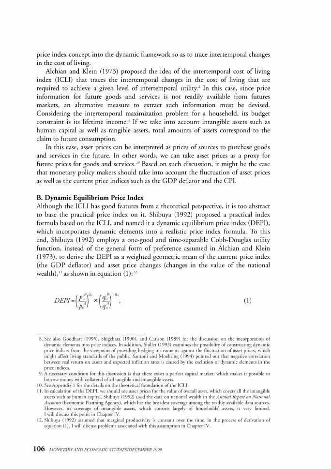
B. Dynamic Equilibrium Price IndexAlthough the ICLI has good features from a theoretical perspective, it is too abstractto base the practical price index on it. Shibuya (1992) proposed a practical index formula based on the ICLI, and named it a dynamic equilibrium price index (DEPI),which incorporates dynamic elements into a realistic price index formula. To thisend, Shibuya (1992) employs a one-good and time-separable Cobb-Douglas utilityfunction, instead of the general form of preference assumed in Alchian and Klein(1973), to derive the DEPI as a weighted geometric mean of the current price index(the GDP deflator) and asset price changes (changes in the value of the nationalwealth),11 as shown in equation (1):12

p0B α0 q0

B 1–α0

DEPI = —— × —— , (1)( p0A) (q0

A)


8. See also Goodhart (1995), Shigehara (1990), and Carlson (1989) for the discussion on the incorporation ofdynamic elements into price indices. In addition, Shiller (1993) examines the possibility of constructing dynamicprice indices from the viewpoint of providing hedging instruments against the fluctuation of asset prices, whichmight affect living standards of the public. Santoni and Moehring (1994) pointed out that negative correlationbetween real return on assets and expected inflation rates is caused by the exclusion of dynamic elements in theprice indices.

9. A necessary condition for this discussion is that there exists a perfect capital market, which makes it possible toborrow money with collateral of all tangible and intangible assets.

10. See Appendix 1 for the details on the theoretical foundation of the ICLI.11. In calculation of the DEPI, we should use asset prices for the value of overall asset, which covers all the intangible

assets such as human capital. Shibuya (1992) used the data on national wealth in the Annual Report on NationalAccounts (Economic Planning Agency), which has the broadest coverage among the readily available data sources.However, its coverage of intangible assets, which consists largely of households’ assets, is very limited. I will discuss this point in Chapter IV.

12. Shibuya (1992) assumed that marginal productivity is constant over the time, in the process of derivation ofequation (1). I will discuss problems associated with this assumption in Chapter IV.

where α0 = ρ/(1 + ρ), and α0 and ρ represent the weight for the current goods andservices, and time preference, respectively.13

III. Asset Prices as a Leading Indicator of Inflation

In this chapter, I compute the DEPI by following the methodology in Shibuya(1992), and examine the information content of asset prices as a leading indicator of inflation.

A. Calculation of DEPII calculate the DEPI by following the methodology described in Appendix 2 of Shibuya (1992), where the weights for the GDP deflator and national wealth (hereafter, aggregate asset price index) are assumed to be 0.03 and 0.97, respectively.Figure 1 plots the movements of the DEPI from 1957 to 1997.14

This figure shows the large divergence between the DEPI and the GDP deflatorduring the late 1960s, the early and late 1970s, and the early 1980s. Focusing on thedevelopment since the mid-1980s, the DEPI rose sharply from 1986 to 1990, whilethe GDP deflator remained relatively stable, and then the growth rate of the DEPIturned negative from 1991. During this period, the inflation rate in the GDP deflatoraccelerated until 1991, and the inflation rate was subdued from 1992. Such devel-opment of the DEPI might be interpreted as an understatement of the inflationarypressure in the late 1980s and the deflationary pressure from the early 1990s.15

107


13. α0 can be written as αt = (1 + ρ)–t/∑∞s =0(1 + ρ)–s in general form, and are the normalized factors of time preference,

which add up to one. Thus, when we calculate the DEPI on a monthly and quarterly basis, we have to use therate of time preference transformed into a monthly and quarterly basis.

14. I will discuss the appropriateness of the DEPI weights estimated in Shibuya (1992) in Chapter III.15. Shibuya (1992, 1995) pointed out that the large fluctuation of the DEPI suggested a phenomenon of disequilibrium

dynamics in the economy.

–10

–5

0

5

10

15

20

25

30

1957

Note: For the details of the calculation method of the DEPI, see Shibuya (1992).Source: Economic Planning Agency, Annual Report on National Accounts.

59 61 63 65 67 69 71 73 75 77 79 81 83 85 87 89 91 93 95 97

DEPIGDP deflator

Changes from the previous year, percent

Figure 1 DEPI and GDP Deflator

B. Statistical Relationship between Asset Prices and InflationNext, I statistically test the hypothesis that asset prices are a leading indicator of inflation. To this end, I conduct two types of empirical exercises. First, I check theGranger causality among various macroeconomic indicators, including the GDPdeflator and aggregate asset price index, with various setups of vector autoregression(VAR) models. Second, I examine the robustness of Granger causality from assetprices to the GDP deflator over the time with rolling regression across the full sample period.1. Granger causality among various setups of VAR modelsFirst, I check the Granger causality from asset prices to inflation in various setups of VAR models.

The variables used in the VAR models are as follows: (1) first log difference of theGDP deflator (DLCP); (2) first log difference of the aggregate asset price index(DLAP); (3) first log difference of real GDP (DLRY); (4) long-term interest rate(long-term prime lending rate, LR); and (5) first log difference of M2+CD (DLNM).All the series are annual basis, since the aggregate asset price index is available in onlyannual basis, and the estimation period is from 1957 to 1997.

Using these variables, I examine the robustness of Granger causality from theaggregate asset price index to the GDP deflator in three setups of VAR models: (1) two-variable VAR model with only the GDP deflator and aggregate asset priceindex; (2) four-variable VAR model with the GDP deflator, aggregate asset priceindex, real GDP, and long-term interest rate; and (3) five-variable VAR model with all the above variables. In all three VAR models, one-year lags are chosen by the criteria of minimizing the Akaike’s information criteria (AIC).

Table 1 summarizes the results for Granger causality test in three setups of VARmodels. In all cases, the aggregate asset price index Granger causes the GDP deflatorat least at the 5 percent statistical significance. On the contrary, the GDP deflatordoes not Granger cause the aggregate asset price index, except for the five-variableVAR model at 20 percent significance.

These results indicate that asset price fluctuations contain specific informationabout the future price movement, suggesting the potential usefulness of asset prices asan information variable in Japan. 2. Granger causality from asset price to inflation over timeNext, I conduct the second empirical exercise to check the robustness of the Grangercausality from the asset prices to the inflation over time. To this end, I conduct three types of rolling regressions on the aforementioned five-variable VAR modelwith 15-year, 20-year, and 25-year sample periods.


[3] Five-Variable VAR Estimation

Dependent Independent variablesvariable DLCP DLAP DLRY LR DLNM

DLCP 5.620 4.959 0.000 0.033 0.956(0.024) (0.033) (0.998) (0.857) (0.335)

DLAP 1.768 6.773 0.386 0.006 3.130(0.193) (0.014) (0.539) (0.937) (0.086)

DLRY 2.385 3.152 5.234 0.201 6.116(0.132) (0.085) (0.028) (0.657) (0.019)

LR 0.274 6.671 0.005 98.183 0.191(0.604) (0.014) (0.944) (0.000) (0.665)

DLNM 0.988 0.055 0.000 0.702 23.310(0.327) (0.816) (1.000) (0.408) (0.000)

Notes: 1. M2+CD is connected series of the followingtwo series: (1) annual average of outstandingat the end of each month in 1956–69; and (2) annual average of average outstanding ofeach month in 1970–97.

2. Figures in the table are F-values and P-values(in the parentheses).

Sources: Bank of Japan, Economic Statistics Annual;Economic Planning Agency, Annual Reporton National Accounts.

109


Table 1 Granger Causality Test with Different Setup of VAR Models

[1] Two-Variable VAR Estimation

Dependent Independent var.variable DLCP DLAP

DLCP 15.749 21.024(0.000) (0.000)

DLAP 0.171 29.893(0.682) (0.000)

[2] Four-Variable VAR Estimation

Dependent Independent variablesvariable DLCP DLAP DLRY LR

DLCP 7.282 10.549 0.598 0.519(0.011) (0.003) (0.444) (0.476)

DLAP 0.798 16.529 0.353 0.982(0.378) (0.000) (0.556) (0.328)

DLRY 0.807 0.256 20.835 2.850(0.375) (0.616) (0.000) (0.100)

LR 0.435 11.326 0.068 133.663(0.514) (0.002) (0.796) (0.000)

Granger’s causalitySignificant at 1 percent level: lead lagSignificant at 5 percent level: lead lagSignificant at 10 percent level: lead lagSignificant at 20 percent level: lead lag

DLAPDLCP

LR

DLAPDLCP

DLRY

DLNM

DLAPDLCP

DLRY

LR

Figure 2 shows the estimation results for the Granger causality from asset prices toinflation over time. The Granger causality from the aggregate asset price index to the GDP deflator is highly significant in the earlier sample periods. However, it isincreasingly insignificant in the sample periods beginning in the mid-1960s and later on.


F-value

Beginning of sample period

1 percent critical value


0

1412108642

1958 59 60 61 62 63 64 65 66 67 68 69 70 71 72 73 74 75 76 77 78



Beginning of sample period1958 59 60 61 62 63 64 65 66 67 68 69 70 71 72 73

02468

101214

F-value

[2] 20-Year Rolling Regressions


0

2

4

6

8

10

1958 59 60 61 62 63 64 65 66 67 68 69 70 71 72 73 74 75 76 77 78 79 80 81 82 83

F-value

Beginning of sample period


Figure 2 Granger Causality from Asset Price to GDP Deflator over Time


This result suggests that the usefulness of asset prices as an information variablefor inflation development depends on the macroeconomic environments. As a result,it is important to examine the factors behind the asset price fluctuations to extract ameaningful policy implication.

IV. Practical Problems in the DEPI

In this chapter, I examine the practical problems inherent in the DEPI, which makeit less attractive to employ as a target indicator.

A. Appropriateness of Weight for Asset PricesThe weight for the current price index in the DEPI (α0) is calculated from the timepreference (ρ), based on the formula of α0 = ρ/(1 + ρ). Shibuya (1992) employed the modified golden-rule (equilibrium condition of neoclassical growth model withconsidering the optimization behavior of households)16 to estimate this parametervalue. In more detail, the rate of time preference is estimated as 0.03, deducting therate of depreciation as 0.06, the growth rate of labor as 0.01, the rate of techno-logical progress as 0.03 from the real return on assets as 0.13, thus implying that the weights for the current price index and the asset prices are equal to 0.03 and0.97, respectively.

Although the price index formula for the DEPI is the weighted geometric meanof the current price index and asset prices, the movement of the DEPI is almost identical to that of asset prices, because the weight for asset prices is very close to one.As a result, if the DEPI is employed to evaluate the inflation development, it isalmost equivalent to look at the asset price movement.

Moreover, the recent estimation results for the consumption-based capital assetpricing model (CAPM) suggest the possibility of overstatement of the current inflation, even if time preference is assumed as 0.03. For example, Hamori (1996)estimated the Euler equation by assuming the general form of time-separable utilityfunction, and obtained a time preference (ρ) around 0.01.17 If this parameter value is employed, the weights for current price and asset price are 0.01 and 0.99, respectively. Therefore, the weight for asset prices is likely to be much larger, sincethis result holds regardless of the property of the production function.

111


16. For the details of modified golden rule, see, for example, Barro and Sala-i-Martin (1995).17. In general, time preferences are estimated as an inverse number of gross rate of time preference (1/(1 + ρ)) in the

consumption Euler equation. Estimation results with monthly data shown in Hamori (1996) range from 0.985to 0.995. These figures correspond to the time preference of 0.01 on an annual basis.

From the viewpoint of supporting the DEPI, it must be reasonable that the DEPIallocates the very large (small) weight for the asset prices (the current prices), basedon the intertemporal optimization behavior of economic agents. However, such an argument misses the critical point that reliability of asset price statistics is very low. While the current price indices are also affected by measurement errors, theirreliability is by far higher than asset price statistics.18

Therefore, it seems quite difficult to construct a reliable price index that includesasset price information. Putting large weight on the asset prices cannot be rational-ized without considering the large difference in the reliability of statistics. This pointwill be examined in more detail below.

B. Reliability of Asset Price Statistics1. Coverage of statisticsThe ICLI measures changes in the current and future prices of consumption flowsimplied in the asset price fluctuations, while keeping the lifetime utility level


18. See Chapter V for more a detailed discussion on the reliability of the DEPI.

Consider how the weights for the current price index and asset prices will beaffected when the planning horizon of economic agents varies. Table 2 shows thesimulation results. It suggests that the weights for asset prices exceed 0.9 when theplanning horizon of economic agents becomes longer than 10 years, thus indicatingthat the impact of asset price fluctuation becomes dominant.

Table 2 Planning Horizon and Weight for DEPI

Planning Discount factor = 0.03 Discount factor = 0.01horizon Current price Asset price Current price Asset price

2 0.507 0.493 0.502 0.498

4 0.261 0.739 0.254 0.746

6 0.179 0.821 0.171 0.829

8 0.138 0.862 0.129 0.871

10 0.114 0.886 0.105 0.895

20 0.065 0.935 0.055 0.945

30 0.050 0.950 0.038 0.962

40 0.042 0.958 0.030 0.970

50 0.038 0.962 0.025 0.975

60 0.035 0.965 0.022 0.978

70 0.033 0.967 0.020 0.980

80 0.032 0.968 0.018 0.982

90 0.031 0.969 0.017 0.983

100 0.031 0.969 0.016 0.984

∞ 0.029 0.971 0.010 0.990

constant. In this case, it is crucial to emphasize that the ICLI must cover all assets,which are sources of present and future consumption, such as tangible and intangi-ble, financial and nonfinancial, and human and nonhuman assets. Nevertheless, eventhe National Wealth Statistics, which have the broadest coverage among the assetprice statistics and are used in compiling the DEPI, do not include human capital.19

The reasons why no comprehensive asset price statistics, which cover human capital, exist are as follows. First, human capital is never traded in the markets, and itis quite difficult to estimate its market value. Second, human capital investment has along development period, and opportunity cost is an important factor for humancapital investment decisions. Third, it is not possible to make a bank loan contractwith collateral of human capital because of an imperfection in capital markets.

Now we try to make some rough estimates on the human capital value, in orderto examine the coverage of currently available asset price statistics. The calculation isbased on the assumption that the value of human capital (WH ) is equivalent to thepresent discounted value of labor income (YL ) under the following conditions:20

(1) growth rate of future labor income (g ), depreciation rate of human capital (d ),and discount rate of future income (r ) are all constant over time; (2) gross growthrate of labor income is equal to the product of gross depreciation rate of human capi-tal and gross discount rate; and (3) population composition and human capitalinvestment pattern are constant over time.

In this case, value of human capital, which is calculated as the present discountedvalue of labor income with average expected job tenure of n -year, is

1 + g 1 + g 2 1 + g n

WH = YL —————— +YL —————— + . . . YL —————— .(2)

(1 + d )(1 + r ) ((1 + d )(1 + r )) ((1 + d )(1 + r ))= nYL

According to the System of National Accounts in Japan, the compensation ofemployees was ¥286 trillion in 1997. If we assume that average expected job tenure is25 years, the value of human capital is calculated as ¥7,157 trillion in 1997 fromequation (2).21

113


19. Ishikawa (1991) provides an extensive survey of the issues related with human capital. 20. The following estimation methodology is taken from Iwata (1992). In addition, there exist other types of estima-

tion methods such as summation of human capital investment, and using an estimated consumption functionbased permanent income hypothesis.

21. Takayama (1992) applies individual data of National Survey of Family Income and Expenditure to estimate thevalue of households’ human capital in 1984 at ¥4,406 trillion. It corresponds to ¥5,146 trillion on a 1994-yearbasis after adjusting for inflation between 1984 and 1994. This figure is judged as approximately equivalent tothe estimates in this paper, because the estimates in Takayama (1992) do not cover the one-person family.

2. Accuracy of price informationAnother problem of asset price statistics is that their accuracy is insufficient for quan-titative analysis. For example, land, which is a typical tangible asset, is characterizedby its diversity and variety. In practice, there are various evaluations of land prices,ranging from actual traded prices to the Officially Published Land Prices, and it isquite difficult to say which price indicates fair prices. In this case, although it may be possible to apply a hedonic approach to estimate quality-adjusted price changes,limited data availability would make such research quite difficult.22

3. Changes in composition of asset holdingsIn constructing an aggregated asset price indicator, it is also difficult to adjust thechanges in asset composition over time. Table 4 shows an asset and debt compositionin the consolidated balance sheet for Japan over time, and two points should benoted. First, both the asset and debt sides of the national balance sheet for Japanexpanded more rapidly than the national wealth (deducted debt and equity fromtotal assets). The ratio of total assets (equal to the sum of total debt and net worth) tothe nominal GDP increased to 16.6 in 1990 from 8.1 in 1970, and declined to 14.6in 1997. During the same time period, net worth rose from 4.0 in 1970 to 8.2 in1990 and declined to 6.4 in 1997. Second, looking at the composition of assets anddebt, the weight of financial assets, and debt excluding equity increased.


When we sum up the above estimated value of human capital and the value ofnonhuman capital assets in the System of National Accounts, total net asset value ofhouseholds reached ¥8,854 trillion in 1997 (Table 3). The table also shows that theratio of nonhuman and human capital is about one to three, and the relative impor-tance of human capital is high. This indicates that the coverage of the NationalWealth Statistics is just 25 percent of the total assets in the household sector.

Table 3 Balance Sheet for Households in 1997

¥ trillions, percent

Nonhuman capital 2,654 ( 28.4)

Net fixed assets 303 ( 3.2)

Land 1,068 ( 11.4)

Financial assets 1,222 ( 13.1)

Others 61 ( 0.6)

Debt 401 ( 4.3)

Net worth 2,187 ( 23.4)

Human capital 7,157 ( 76.6)

Net total assets 9,344 (100.0)

National wealth 3,241Notes: 1. Figures on human capital are the author’s estimation.

2. Net total assets are sum of net worth and human capital.3. National wealth covers nonfinancial incorporated enterprises, financial

institutions, and general government, in addition to households.Source: Economic Planning Agency, Annual Report on National Accounts.

22. See Suzuki and Ohta (1994) for an application of the hedonic approach to land price analysis. In addition, thereare estimates such as Ito and Hirono (1993) and Kasuga (1996) for housing prices and rents.

The DEPI focuses on the changes in net national wealth to trace the fluctuationsin the aggregated asset value as the sources of future consumption expenditure.However, it should be noted that changes in the net national wealth might reflect theimpact of changes in the composition of assets and debt.

C. Policy Implications and Sources of Asset Price Fluctuation1. Dispersion from fundamentalsBased on the discounted present value formula, which is the basic theoretical frame-work for asset pricing, asset price is equal to the present discounted value of futureflow of its income. Profit maximization of the firm indicates that its marginal revenuecorresponds to its marginal productivity of assets. Therefore, if we assume that marginal productivity of capital (MPK ), nominal interest rate (r ), and expected rateof inflation (π) are all constant over time, real asset price (q /p) is determined as

q /p = MPK /(r – π). (3)

This equation implies that expected return on assets and expected nominal rate determine the fluctuation of real asset price.

115


Table 4 Consolidated Accounts for Japan

¥ trillions, percent

1970 80 90 97

Reproducible tangible assets 121 ( 20.5) 592 ( 22.4) 1,053 ( 14.8) 1,387 ( 18.7)

Non-reproducible tangible assets 174 ( 29.4) 745 ( 28.2) 2,420 ( 33.9) 1,729 ( 23.3)

Financial assets 296 ( 50.1) 1,305 ( 49.4) 3,663 ( 51.3) 4,306 ( 58.0)

Total assets 591 (100.0) 2,642 (100.0) 7,137 (100.0) 7,422 (100.0)

Debt (excluding equity) 266 ( 45.1) 1,177 ( 44.6) 3,008 ( 42.1) 3,810 ( 51.3)

Equity 28 ( 4.7) 125 ( 4.7) 607 ( 8.5) 371 ( 5.0)

Net wealth 296 ( 50.2) 1,340 ( 50.7) 3,522 ( 49.4) 3,241 ( 43.7)

Ratio to nominal GDP 4.0 5.6 8.2 6.4

Total debt and national wealth 591 (100.0) 2,642 (100.0) 7,137 (100.0) 7,422 (100.0)

Ratio to nominal GDP 8.1 11.0 16.6 14.6

Source: Economic Planning Agency, Annual Report on National Accounts.

Figure 3 plots the time series of changes in real price of net national wealth, realGDP growth,23 and changes in expected real interest to examine the relationshipbetween asset price and fundamentals. It shows that real asset price changes almostcorrespond to the movements in fundamentals. The changes in real asset price have apositive correlation with real GDP growth, and a negative correlation with expectedchanges in the real interest rate.


–25

–20

–15

–10

–5

0

5

10

15

20

25

1957 59 61 63 65 67 69 71 73 75 77 79 81 83 85 87 89 91 93 95 97

Percent

National wealth growthReal GDP growthChanges in ex post long-term real interest rates

Note: Ex post long-term real interest rates correspond to the long-term prime lending rate deducted by the changes of the GDP deflator.Sources: Economic Planning Agency, Annual Report on National Accounts; Bank of Japan, Financial and Economic Statistics Monthly.

Figure 3 Asset Price Fluctuation and Fundamentals

However, it is also true that the degree of correlation between the real asset price and fundamentals varies over time. For example, from the late 1980s, Japanexperienced tremendous fluctuation of asset prices, which is much larger than thefluctuation implied by the fundamental variables such as real GDP growth andexpected changes in the real interest rate.

Prolonged deviation of asset price from its fundamental value is often called abubble. Even if investors are perfectly rational, the actual stock price may contain a bubble element and, therefore, there can be a divergence between the asset priceand its fundamental value.24 In general, asset prices reflect investors’ expectationsabout the future, and such expectations seem to have played an important role in sustainability of bubbles. In this case, it is impossible to extract information on futureinflation rates of goods and services from the asset prices.

23. Real GDP growth can be thought of as a proxy for profitability of assets on a real basis. 24. In order to exclude the bubble path, it is assumed that asset prices will not diverge to infinity. See, for example,

Blanchard and Watson (1982) for the discussion on the asset price bubble.

However, in the case of the collapse of the bubble, the negative impact on theeconomy will increase, as the overvaluation of asset prices continues, thus resulting inlarger swings in business conditions. In this sense, the rise in the DEPI due to theovervaluation of asset prices may be viewed as a signal for monetary tightening. 2. Adjustment for changes in marginal productivity of assetsThe above discussion assumes a static expectation on the marginal return on assets.That is, it assumes that constant rates of economic growth or marginal return onassets continue over time. Indeed, Shibuya (1992) assumes that marginal return onassets is constant over time in order to compute the DEPI with readily available data.

However, the increases in land prices do not necessarily imply the increase in thefuture prices of services that will be produced by land. The increases in land pricesmay reflect the higher productivity of land in the future, which is the consequence oftechnological innovations, such as advances in construction technology of the higherskyscrapers and smart buildings.

Now suppose that the changes in the marginal productivity of assets occurbetween the economic conditions A and B. Then the DEPI defined equation (1) ismodified as follows:

p0B α0 q0

B/MPK B 1–α0

DEPI = —— × ————— . (4)( p0A ) (q0

A/MPK A )This equation implies that asset prices must be deflated by their marginal

productivity to convert them into the asset prices in efficiency unit when we try toextract information on the future prices of products and services. For example, thechanges in the marginal productivity must be deducted from the changes in the unitprice of land.

Figure 4 plots the year-to-year changes of land prices in Japan by usage. In general, land prices show a similar trend across usage, and no significant changes inthe relative prices are observed. In this case, as mentioned above, it is necessary to

117


–30

–20

–10

0

10

20

30

40

50

Average of all purposeCommercial landResidential land

1970 72 74 76 78 80 82 84 86 88 90 92 94 96

Changes from a year earlier, percent

Source: Japan Real Estate Institute, Urban Land Price Index.

Figure 4 Land Prices by Use

detect the asset price changes measured in the efficiency unit to extract meaningfulinformation. However, such changes in marginal productivity of assets are notdirectly observable, nor does a readily available proxy exist. Therefore, it is necessaryto estimate an aggregate production function to compute the marginal productivityin a rigorous way. Still, it is difficult to estimate the marginal productivity for different assets, and accumulation of time-series data is required to deduct the structural breaks with econometric methodology.

In addition, even though the current marginal productivity can be traced properly, it might be the case that deviation from the proxy for the fundamentalsoccurs under the expectations on the higher marginal return on assets, reflecting thefuture innovations. In this case, the difficult question arises to judge in advancewhether such asset price increases are phenomena of euphoria.

In summary of the above discussion, when we employ the DEPI as one of thecore economic indicators for monetary policy judgment, it is necessary for monetarypolicy makers to access the possibility of unobserved structural breaks that provokethe substantial changes in the marginal productivity of the economy.

In the monetary policy regime of inflation targeting, which most clearly definesthe policy objectives in terms of inflation measures, escape clauses are introduced topermit central banks to temporarily deviate from the targeted range of inflation ratesin the case of significant supply shocks, such as remarkable rises in oil prices and natural disasters.25 In this context, the shift in the marginal productivity of assets,which is interpreted as the structural change in the supply-side of the economy,should be included in the escape clauses, if a central bank adopts an inflation targetfor the DEPI for its monetary policy framework. In addition, the validity of marketexpectations, such as the possibility of bubble and euphoria, should be examined toextract the policy implication from the changes in the DEPI properly.

Considering these limitations, it is inappropriate for monetary policy makers toemploy the DEPI as one of the core indicators for monetary policy judgment.


25. See Bank of Japan (1995), Bernanke et al. (1999), and Leiderman and Svensson (1995) for the details of inflation targeting.

V. Optimal Inflation Measure in Practice

In this chapter, based on the above discussion, I will explore the question of what theoptimal inflation measure for monetary policy is in practice.

A. Reliability of DEPIIn order to discuss the optimal inflation measures, it is important to obtain the feasible combinations between the weight for asset prices and the observation errorsin the inflation measures. To this end, I perform a simulation on the observationerrors in the DEPI to analyze its reliability under the following conditions.

(1) I assume the distributions of changes in price index and asset price follow the nor-mal distribution. This implies that price index and asset price levels follow thelognormal distribution. As a result, the DEPI follows the lognormal distribution,since the DEPI is defined as the geometric mean of price index and asset price.

(2) I assume that observation errors in the GDP deflator are equal to those for theCPI, estimated in Appendix 2 at the level of 0.1 percent annually. In addition,I also assume three levels of observation errors in asset prices, that is, 10, 100,and 1,000 times that for the CPI.26

(3) I assume five levels of correlation between the GDP deflator and asset price fluctuations. The coefficient of correlation is 0.00, 0.10, 0.25, 0.50, and 1.00, respectively.27

(4) I assume six combinations of the weights for the GDP deflator and assetprice: 0.01:0.99, 0.03:0.097, 0.10:0.90, 0.25:0.75, 0.50:0.50, and0.75:0.25, respectively.

(5) Simulation results are compared with the benchmark of the estimated observation errors in the CPI of the lowest aggregation level at 0.1 percent per annum.28

119


26. According to the estimated observation errors of the CPI in Appendix 2, the observation errors increase as theaggregation levels in data become high. The estimate of the highest aggregation data reaches 1.1 percent perannum, while that of the lowest aggregation data remains just 0.1 percent per annum. Therefore, estimatedobservation errors vary in accordance with the data aggregation level, by as much as 10 times between the lowestand highest cases. This suggests that estimations with highly aggregated data enlarge the observation errorsbecause of the deterioration in the accuracy of price information. Since asset prices are characterized by the diversity, their accuracy is far lower than that of the CPI price survey. Based on the above consideration, the simulation in this paper assumes the three different levels of observation errors in the asset prices: 10, 100, and1,000 times the observation errors in the CPI.

27. Coefficients of correlation between the GDP deflator and asset price are 0.27 in 1970 to 1994, and 0.11 in 1980to 1994.

28. This criterion means that the 95 percent confidence range for the observed inflation rate is 0.2 percent in boththe upper and lower sides, when changes in the CPI follow the normal distribution process. For example, whenthe year-to-year inflation rate is 2.0 percent, there will be a true value between 1.8 and 2.2 percent with the probability of 95 percent.

Table 5 reports the simulation results, and shows the large observation errors,close to that of asset prices, when the weights for asset prices exceed 0.9. Minimumvalue among the simulated observation errors in the DEPI is 0.5 percent per annum,and it is 10 times larger than that of the GDP deflator. Considering the above examination on the accuracy of the National Wealth Statistics, actual observationerrors in the DEPI are expected to be far larger than this minimum result. Inaddition, suppose that the achievement of the monetary policy objective is measuredby the divergence from the targeted inflation rate, and the required confidence rangeis 0.5 percent on both the upper and lower sides.29 All the simulation results exceedthe allowance.


29. Those countries that adopt inflation targeting as the monetary policy framework set an allowance range of 1 percent around the targeted inflation rates. In general, the reason why such targeting ranges are set is that thereis a limitation in the controllability of inflation by monetary policy against the business cycle fluctuation andexternal shocks. Therefore, we assume the maximum allowance level of the observation errors is half that of the ordinary targeting ranges.

Table 5 Simulation Results for Observation Errors in the DEPI

Weights Assumption on correlation

Current price Asset price 0.00 0.10 0.25 0.50 1.00

Case 1: Observation errors in asset price = 10 times the current price

0.01 0.99 0.995 0.995 0.995 0.996 0.996

0.03 0.97 0.985 0.985 0.986 0.987 0.988

0.10 0.90 0.949 0.950 0.952 0.954 0.959

0.25 0.75 0.867 0.870 0.873 0.878 0.889

0.50 0.50 0.711 0.714 0.719 0.728 0.745

0.75 0.25 0.507 0.511 0.517 0.526 0.543

Case 2: Observation errors in asset price = 100 times the current price

0.01 0.99 9.950 9.950 9.950 9.950 9.951

0.03 0.97 9.849 9.849 9.850 9.850 9.852

0.10 0.90 9.487 9.488 9.489 9.492 9.496

0.25 0.75 8.660 8.663 8.666 8.671 8.682

0.50 0.50 7.071 7.075 7.080 7.089 7.107

0.75 0.25 5.001 5.004 5.010 5.019 5.038

Case 3: Observation errors in asset price = 1,000 times the current price

0.01 0.99 99.499 99.499 99.499 99.499 99.500

0.03 0.97 98.489 98.489 98.489 98.490 98.492

0.10 0.90 94.868 94.869 94.871 94.873 94.878

0.25 0.75 86.603 86.605 86.608 86.613 86.624

0.50 0.50 70.711 70.714 70.720 70.728 70.746

0.75 0.25 50.000 50.004 50.009 50.019 50.038

As the weight for asset prices increases, the observation errors in the DEPI contin-uously rise. Therefore, their feasible combinations, “the inflation measure frontier,”are downward sloping and convex to the lower right. In addition, the indifference

B. Optimal Weight Allocation to Asset Prices in PracticeNow I will investigate the optimal combination between the weight for asset pricesand the observation errors in the DEPI.

Figure 5 plots the changes in the estimated observation errors in the DEPI inresponse to varying the weights between asset prices and the current price index.30 Inthis figure, the vertical and horizontal axes correspond to the weight assigned to theasset prices and the estimates of the observation errors in the DEPI, respectively.

121


Inflation measure frontier

Weight for asset prices1.2

1.0

0.8

0.6

0.4

0.2

00 2 4 6 8 10 12

Observation errors, percent

Assumption1. Observation errors for asset prices 　are 100 times larger than those of 　current price index.2. There is no correlation between 　fluctuations of asset prices and 　current price index.

Optimal solution

Indifference curve

Figure 5 DEPI Weight and Observation Errors

30. In Figure 5, the simulation is conducted under the assumptions that (1) observation errors in the asset price are100 times more than those for the price index; and (2) there is no correlation between the fluctuation of assetprices and the price index. It should be noted that simulation results shown in Table 5 suggest that simulationresults will not be influenced if there exists correlation between the fluctuation of asset prices and price index.

curve for the desirable inflation measures in terms of the weight for the asset pricesand the observation errors is also downward sloping and convex to the lower right,since there exists a trade-off between the weight for the asset prices and the observa-tion errors (dashed curve in the figure). On the one hand, increased weight for theasset prices is desirable because the DEPI will reflect much more information onfuture inflation expectations. On the other hand, increased observation errors willreduce the credibility of inflation measures.

Both the indifference curve and the inflation measure frontier are downward sloping and convex to the lower right. Thus, if the indifference curve is tangent tothe inflation measure frontier from the inside, the tangency point will be the desirable combination of weight for the asset price and observation errors. However,if the DEPI is employed as a target indicator for monetary policy, the cost for theincrease in the observation errors will rise, as the weight for the asset prices increases.This implies that the slope of the indifference curve is steeper than that of the inflation measure frontier, thus producing the corner solution shown in Figure 5. In this case, the desirable target indicator for the monetary policy will be the conven-tional price index, which allocates the zero-weight for asset prices in the DEPI. Inother words, although there is a reasonable theoretical foundation for supposing thatthe DEPI allocates a large weight for asset prices, it is difficult to employ it as a coreindicator for the monetary policy judgment due to the extremely low accuracy of thereadily available data.

VI. Conclusion

In this paper, I examined the possibility of constructing a reliable inflation measurethat reflects both the current inflation and asset prices from the theoretical and practical viewpoints. Such an inflation measure, the dynamic equilibrium price index(DEPI), is the extension of the conventional price index concept into the dynamicframework. Although the concept of the DEPI is highly evaluated from the view-point of theoretical consistency, it is difficult for monetary policy makers to expectthe DEPI to be more than a supplementary indicator for inflation pressures. This isbecause such modification of the conventional price indices is hardly operational.

The first problem inherent in the DEPI is that asset price changes do not neces-sarily predict future price changes because there are a lot of sources for asset pricefluctuations besides the private-sector expectations for the future course of inflation,such as bubble elements of private-sector expectations and structural changes in theeconomy. Therefore, if the DEPI is employed as one of the core indicators for mone-tary policy judgment, monetary policy makers will be faced with the difficulty that itis very hard to extract from the DEPI an appropriate policy implication in practice.

The second problem is the appropriateness of large weight for asset prices in theDEPI. The DEPI is defined as the geometric weighted mean of the current priceindex and asset price, and its weight for asset price is almost equal to one, while thatfor the current price index is almost zero. From the theoretical viewpoint, it is reason-able to assign the large (small) weight for the asset prices (the current price index),


reflecting the dynamic optimization of economic agents. However, such discussionmisses the practical viewpoint that reliability of asset price statistics is quite low.Although the conventional price indices are also affected by measurement problems,their reliability is much higher than asset price statistics, implying a difficulty in constructing a reliable price index that includes asset prices.

The DEPI will be quite a similar indicator to asset prices, as far as one accepts thetheoretical weights for the current price index and asset prices. If asset prices arejudged to be inappropriate as a policy target indicator, and are limited as informationvariables for monetary policy judgment, it is enough to monitor both the currentprice indices and the asset prices separately.

In this context, it should be noted that, as Kindleberger (1995) pointed out, thereare no cookbook rules for policy judgment, and it is inevitable for monetary policyauthorities to make a discretional judgment.31

The above conclusion implies that the argument by Bernanke and Woodford(1997) is not a serious problem for monetary policy makers in practice. They pointout that it is not the case that monetary policy makers can respond mechanically toprivate-sector inflation forecasts, since it leads to indeterminacy of rational expecta-tion equilibria. In this case, the asset prices are one of the most likely indicators formonetary policy makers to extract the information on the future course of inflationdevelopments.

However, considering the limitation in asset prices discussed in this paper, it isnecessary to make a discretionary judgment to extract an appropriate policy implica-tion from the asset price fluctuations. Therefore, it is not practically feasible toassume a mechanical rule to respond to the asset price fluctuations.32

123


31. Kindleberger (1995) comments on this point as follows:When speculation threatens substantial rises in asset prices, with a possible collapse in asset markets later, andharm to the financial system, or if domestic conditions call for one sort of policy, and international goalsanother, monetary authorities confront a dilemma calling for judgment, not cookbook rules of the game.

32. A similar argument will hold if monetary policy makers employ survey data on the private-sector forecast forinflation as a targeted variable. This is because such survey data are likely to reflect the private sector’s belief ofunseen structural changes in the economy. In this case, it does not seem to be practically feasible for monetarypolicy makers to mechanically react to the private-sector forecasts for inflation.

APPENDIX 1: FORMULATION OF DYNAMICALLY EXPANDEDPRICE INDEX

As an inflation measure for incorporating the dynamic elements of price fluctuation,Alchian and Klein (1973) proposed the idea of an intertemporal cost of living index(ICLI) that traces “the intertemporal changes in the cost of living that is required toachieve a given level of intertemporal utility.”

Assuming that consumer preference depends on both the current and future consumption expenditure as the following utility function:

U = U (x A11, . . . x A

n1, . . . , xitA, . . .) for i = 1, . . . , n ; t = 1, . . . ∞, (A.1)

where xitA represents the consumption expenditure for good i at time t with economic

condition of A. The budget constraint of the consumer corresponds to the total assets (W A) that

cover the tangible and intangible assets as follows:

∞ n m

W A = ∑∑pitA xit

A = ∑qjAyj

A, (A.2)t=1 i=1 j=1

where pitA, qj

A, yjA represent the current price of good i at time t under economic

condition A,33 and price and quantity of asset j at time t under economic condition A.Suppose that the current price of the current or future goods change, and the new

economic condition B is realized. As a result, suppose also that the required asset valuefor the consumer to achieve the same utility level under the economic condition Abecomes W B. The ICLI between the economic conditions A and B is defined as

∞ n m

∑∑pitBxit

B ∑qjByj

B

W Bt=1 i=1 j=1ICLI AB = —— = ———— = ———. (A.3)

W A ∞ n m

∑∑pitAxit

A ∑qjAyj

A

t=1 i=1 j=1

Shibuya (1992) formulates the DEPI as a geometric mean of the current priceindex and asset prices by assuming a time-separable utility function in one goodmodel and constant marginal productivity of assets.


33. This is the present value of the future product and service prices discounted by the discounted factor.

APPENDIX 2: APPLICATION OF OLS METHOD TO ESTIMATEOBSERVATION ERRORS IN PRICE INDEX

Appendix 2 shows the estimation procedure and results for the observation errors inthe price index, which are the basic data for the simulation on the observation errorsin the DEPI. First, following Selvanathan and Prasada Rao (1994), I summarize themethodology to estimate the Laspeyres price index and its observation errors fromthe disaggregated data. Then, I estimate the observation errors with four data setswith different aggregation level of the CPI: 10 major group index, subgroup index,item class index, and item index.

Now let p0t xi 0 and pit xi 0 be consumption expenditure to good i at the base period0 and the current period t , respectively, and consider the regression equation as follows:

pit xi 0 = γt p0t xi 0 + εit , i = 1, 2, . . . , n (A.4)

where γt is identical to all good, and εit is a random component. In addition, assuming

E [εit] = 0, cov[εit , εjt] = σt2pi0xi 0δi j , (A.5)

where δi j is Kronecker’s delta. By dividing equation (A.4) by √pi0xi 0, the following equation is derived:

p*it = γt p*i 0 + uit , (A.6)

where p*it = pit √xi 0/pi0, uit = εit/√pi0xi 0. From equation (A.5),

cov[uit , ujt ] = cov[uit , ujt ]/(pi0xi 0) = σt2δi j . (A.7)

Therefore, the ordinary least square (OLS) estimation can be applied. The estimatedcoefficient is

n n n n

γ̂t = ∑p*itp*i 0/ ∑(p*i 0)2 = ∑pit xi 0/ ∑pi0xi 0, (A.8)

i=1 i=1 i=1 i=1

and coincides with the Laspeyres index formula. Thus, the standard error for the estimated coefficient corresponds to the observation error for the price index.

125



Appendix Table 1 Estimation of Observation Errors in the CPI

1991 92 93 94 95 Average

Estimation by item index

Coeff. 1.033 1.050 1.064 1.071 1.070 —

S.E. 0.002 0.002 0.003 0.004 0.005 0.001

R2 0.996 0.992 0.987 0.978 0.971 —

Estimation by item class index

Coeff. 1.032 1.050 1.063 1.071 1.070 —

S.E. 0.003 0.005 0.006 0.007 0.009 0.006

R2 0.997 0.994 0.992 0.986 0.981 —

Estimation by subgroup index

Coeff. 1.032 1.050 1.064 1.071 1.070 —

S.E. 0.005 0.006 0.008 0.011 0.013 0.008

R2 0.995 0.994 0.990 0.981 0.975 —

Estimation by 10 major group index

Coeff. 1.033 1.050 1.063 1.071 1.070 —

S.E. 0.005 0.007 0.010 0.014 0.017 0.011

R2 0.998 0.997 0.994 0.988 0.982 —

Appendix Table 1 shows the estimation results for the item index, item classindex, subgroup index, and 10 major group index in the Japanese CPI.34 The estimated observation error for the CPI is just 0.1 percent per year for the item index,which has the lowest aggregation level. However, the estimates become larger as theaggregation level gets higher: 0.6, 0.8, and 1.1 percent per year for the item classindex, subgroup index, and 10 major group index, respectively. This implies that theobservation errors expand as the accuracy of price survey decreases.

34. Estimation is conducted with the 1990-base CPI.

Alchian, Armen A., and Benjamin Klein, “On a Correct Measure of Inflation,” Journal of Money, Credit,and Banking, 5 (1), 1973, pp. 173–191.

Ball, Laurence, and N. Gregory Mankiw, “Relative-Price Changes as Aggregate Supply Shocks,”Quarterly Journal of Economics, 110 (1), 1995, pp. 161–193.

Bank of Japan, “Inflation Targeting in Selected Countries,” Bank of Japan Quarterly Bulletin, 3 (2),1995, pp. 39–52.

Barro, Robert J., and Xavier Sala-i-Martin, Economic Growth, McGraw-Hill, Inc., 1995.Bernanke, Ben S., and Michael Woodford, “Inflation Forecasts and Monetary Policy,” Journal of Money,

Credit and Banking, 29 (4), 1997, pp. 654–684.———, Thomas Laubach, Fredric S. Mishkin, and Adam S. Posen, Inflation Targeting: Lessons from the

International Evidence, Princeton University Press, 1999. Blanchard, Olivier J., and Mark W. Watson, “Bubbles, Rational Expectations, and Financial Markets,”

in Paul Wachtel, ed. Crises in the Economic and Financial Structure, Lexington Books, 1982, pp. 295–315.

Bockelmann, Horst, “Comments,” in Kuniho Sawamoto, Zenta Nakajima, and Hiroo Taguchi, eds.Financial Stability in a Changing Environment, Macmillan Press, 1995, pp. 498–500.

Borio, C. E. V., N. Kennedy, and S. D. Prowse, “Exploring Aggregate Asset Price Fluctuations acrossCountries: Measurement, Determinants and Monetary Policy Implications,” BIS EconomicPapers No. 40, 1994.

Bruni, Franco, “Comments” in Kuniho Sawamoto, Zenta Nakajima, and Hiroo Taguchi, eds. FinancialStability in a Changing Environment, Macmillan Press, 1995, pp. 501–505.

Carlson, Keith M., “Do Price Indices Tell Us about Inflation? A Review of the Issues,” Federal ReserveBank of St. Louis Review, 71 (6), 1989, pp. 12–30.

Goodhart, Charles A. E., “Price Stability and Financial Fragility,” in Kuniho Sawamoto, ZentaNakajima, and Hiroo Taguchi, eds. Financial Stability in a Changing Environment, MacmillanPress, 1995, pp. 439–497.

Hamori, Shigeyuki, Shouhisha Koudou to Nihon no Shisan Shijo (Consumer Behavior and Japanese AssetMarkets), Toyo Keizai Shimposha, 1996 (in Japanese).

Hoshi, Takeo, “Shihon Shijo no Hukanzen Sei to Kin’yu Seisaku no Hakyu Keiro: Saikin no KenkyuSeika no Tenbo (Imperfection in Capital Markets and Transmission Mechanism of MonetaryPolicy: Review of Recent Studies),” Kin’yu Kenkyu (Monetary and Economic Studies), 16 (1),Institute for Monetary and Economic Studies, Bank of Japan, 1996, pp. 105–136 (in Japanese).

Ishikawa, Tsuneo, Shotoku to Tomi (Income and Wealth), Iwanami Shoten, 1991 (in Japanese). Ito, Takatoshi, and Keiko Nosse Hirono, “Efficiency of the Housing Market,” Monetary and Economic

Studies, 11 (1), Institute for Monetary and Economic Studies, Bank of Japan, 1993, pp. 1–32.Iwata, Kazumasa, “Sutokku Keizai to Zeisei (Stock Economy and Tax System),” Takatoshi Ito and

Yukio Noguchi, eds. Bunseki Nihon Keizai no Suttoku Ka (Analysis on Advance in StockEconomy), Nihon Keizai Shimbunsha, 1992 (in Japanese).

Kasuga, Yoshiyuki, “Shutoken ni Okeru Jutaku no Kousatsu: Mikuro Deita ni Yoru Jutaku Shijou noKenshou (Housing Problems in Metropolitan Area: Examination of Housing Market by MicroData),” Chousa No. 211, Japan Development Bank, 1996 (in Japanese).

Kindleberger, Charles P., “Asset Inflation and Monetary Policy,” BNL Quarterly Review, No. 192,1995, pp. 17–37.

Leiderman, Leonard, and Lars E. O. Svensson, eds. Inflation Targets, CEPR, 1995.Matsushita, Yasuo, “Role of Capital Market and Its Confronting Problems,” Bank of Japan Quarterly

Bulletin, Bank of Japan, 1995, pp. 15–23.Noguchi, Yukio, Baburu no Keizaigaku (Economics on Bubbles), Nihon Keizai Shimbunsha, 1992

(in Japanese). Okina, Kunio, Kitai to Touki no Keizai Bunseki—‘Baburu’ Genshou to Kawase Reito (Economic Analysis

of Expectations and Speculations—‘Bubble’ Phenomena and Exchange Rates), Toyo KeizaiShimposha, 1985 (in Japanese).

127


References

———, Kin’yu Seisaku (Monetary Policy), Toyo Keizai Shimposha, 1993 (in Japanese).Pollak, Robert A., The Theory of the Cost-of-Living Index, Oxford University Press, 1989.Santoni, G. J., and H. Brian Moehring, “Asset Return and Measured Inflation,” Journal of Money,

Credit, and Banking, 26 (2), 1994, pp. 232–248.Selvanathan, E. A., and D. S. Prasada Rao, Index Numbers: A Stochastic Approach, Macmillan Press,

1994.Shibuya, Hiroshi, “Dynamic Equilibrium Price Index: Asset Price and Inflation,” Monetary and

Economic Studies, 10 (1), Institute for Monetary and Economic Studies, Bank of Japan, 1992,pp. 95–109.

———, “Monetary Policy, Banking Crisis, and Disequilibrium Dynamics: Business Cycles withCapital Price Overshooting,” mimeo, 1995.

Shigehara, Kumiharu, “Shisan Kakaku no Hendo to Infureishon ni Tsuite (Asset Price Fluctuation andInflation),” Kin’yu Kenkyu (Monetary and Economic Studies), 9 (2), Institute for Monetary andEconomic Studies, Bank of Japan, 1990, pp. 1–5 (in Japanese).

Shiller, Robert J., Macro Markets, Oxford University Press, 1993.Shiratsuka, Shigenori, “Shisan Kakaku Hendo to Bukka Shisu (Asset Price Fluctuation and Price

Indices),” Kin’yu Kenkyu (Monetary and Economic Studies), 14 (4), Institute for Monetary andEconomic Studies, Bank of Japan, 1996, pp. 45–72 (in Japanese).

———, “Inflation Measures for Monetary Policy: Measuring the Underlying Inflation Trend and ItsImplication for Monetary Policy Implementation,” Monetary and Economic Studies, 15 (2),Institute for Monetary and Economic Studies, Bank of Japan, 1997, pp. 1–26.

———, Bukka no Keizai Bunseki (Economic Analysis of Inflation Measures), University of TokyoPress, 1998 (in Japanese).

———, “Measurement Errors in the Japanese Consumer Price Index,” Monetary and Economic Studies,Institute for Monetary and Economic Studies, Bank of Japan, 17 (3), 1999, pp. 69–102 (this issue).

Suzuki, Kenji, and Makoto Ohta, “A Hedonic Analysis of Land Prices and Rents in the Bubble:Kanagawa Prefecture in Japan for 1986–1988,” Economic Studies Quarterly, 45 (1), 1994, pp. 73–94.

Suzuki, Yoshio, En Defure to Doru Infure (Yen Deflation and Dollar Inflation), Toyo Keizai Shimposha,1995 (in Japanese).

Takayama, Noriyuki, Sutokku Ekonomi (Stock Economy), Toyo Keizai Shimposha, 1992 (in Japanese).


asset price fluctuation and price indices

Documents