Asset Pricing and Sports Betting

Tobias J. Moskowitz∗

ABSTRACT

I use sports betting markets as a laboratory to test behavioral theories of cross-sectional asset pricing anoma-lies. Two unique features of these markets provide a distinguishing test of behavioral theories: 1) the bets arecompletely idiosyncratic and therefore not confounded by rational theories; 2) the contracts have a known andshort termination date where uncertainty is resolved that allows any mispricing to be detected. Analyzingmore than a hundred thousand contracts spanning two decades across four major professional sports (NBA,NFL, MLB, and NHL), I find momentum and value effects that move betting prices from the open to theclose of betting, that are then completely reversed by the game outcome. These findings are consistent withdelayed overreaction theories of asset pricing. In addition, a novel implication of overreaction uncovered insports betting markets is shown to also predict momentum and value returns in financial markets. Finally,momentum and value effects in betting markets appear smaller than in financial markets and are not largeenough to overcome trading costs, limiting the ability to arbitrage them away.

∗University of Chicago, Booth School of Business and NBER. I have benefited from the suggestions and comments of John

Cochrane, Lauren Cohen, Josh Coval, Eugene Fama, Ken French, Xavier Gabaix, Bryan Kelly, Steve Levitt, Gregor Matvos,

Lasse Pedersen, Amit Seru, Jesse Shapiro, John Shim, Richard Thaler, and Rob Vishny, as well as seminar participants at the

SIFR conference in Stockholm, Sweden in August 2013. I also thank John Shim and Brian Weller for outstanding research

assistance. Moskowitz thanks the Center for Research in Security Prices, the Fama Family Chair, and the Initiative on Global

Markets at the University of Chicago, Booth School of Business for financial support. Moskowitz also has an ongoing consulting

relationship with AQR Capital, who has nothing to do with and no interest in sports betting markets.

Correspondence to: Tobias J. Moskowitz, 5807 S. Woodlawn Ave., Chicago, IL 60637. E-mail: tobias.moskowitz@chicagobooth.edu.

The asset pricing literature is replete with various predictors of returns for financial market securities, yet

there remains much debate on their interpretation, which is essential to understanding asset pricing’s role in

the broader economy for risk sharing, resource allocation, and investment decisions. Security characteristics

that predict returns have become the focal point for discussions of market efficiency, where the debate centers

on whether these variables represent compensation for bearing risk in an informationally efficient market, or

whether they represent predictable mispricing due to investor biases and market frictions.

Progress on the efficient markets question is mired by the joint hypothesis problem (Fama (1970)) that

any test of efficiency is inherently a test of the underlying equilibrium asset pricing model. As a result, a

host of rational and behavioral theories for the existence of various return predictors populate the literature.

Rational theories link return premia to aggregate systematic risks (e.g., macroeconomic shocks or proxies

for state variables representing the changing investment opportunity set and marginal utility of investors)

through the stochastic discount factor in an informationally efficient market, while behavioral theories link

returns to investor cognitive errors or biases in a less than perfectly efficient market.

Capital market security returns provide a difficult, if not impossible, empirical laboratory to distinguish

between these broad views of asset pricing since the researcher cannot directly observe marginal utility or

investor preferences, and where both rational and behavioral forces may simultaneously be at work.1

To circumvent the joint hypothesis problem, I propose an alternative asset pricing laboratory—sports

betting markets. The idea is simple. Either our asset pricing models should explain security returns from

all markets, or we need different models for different asset types. If the former is more appealing, then

there are two key features of sports betting markets that provide a direct test of behavioral asset pricing

theory, distinct and not confounded by any rational asset pricing framework: 1) sports bets are completely

idiosyncratic, having no relation to any aggregate risk or risk premia in the economy; 2) sports contracts have

a very short known termination date where uncertainty is resolved by an outcome independent from betting

activity, which allows mispricing to be detected.

For the first feature, the critical point is that I only examine the cross-section of sports betting contracts—

comparing betting lines across games at the same time and even across different bets on the same game.

Aggregate risk preferences and changing risk premia might affect the entire betting market as a whole but

they should have no bearing on the cross-section of games or the cross-section of contracts on the same

1Complicating matters further is the role played by institutional, market, funding, trading, delegation, and regulation con-straints that may also affect prices and interact with rational and behavioral forces to exaggerate, mitigate, or perpetuate returnpatterns.

1

game.2 Hence, rational asset pricing theories have nothing to say about return predictability for these

contracts. On the other hand, sports betting contracts should be subject to the same behavioral biases that

are claimed to drive the anomalous returns in financial security markets. The behavioral models focus on

beliefs or preferences that deviate from rational expectations utility theory regarding generic risky gambles

(see Barberis and Thaler (2003)), and thus pertaining as much to idiosyncratic sports bets as they do to capital

market securities. The cross-section of idiosyncratic sports bets provides a unique asset pricing laboratory

independent of aggregate risk and solely focused on the role of investor behavior and information.

The second key feature of the sports betting contracts is that they have a known, and very short, termi-

nation date, where uncertainty is resolved by outcomes that are independent of investor behavior, providing

a terminal “true” value for each security.3 The exogenous terminal value allows for the identification of

mispricing, providing a stronger test of the behavioral models, which assume prices deviate from their funda-

mental values due to cognitive biases or erroneous beliefs. Once uncertainty is resolved at the terminal date,

however, those mispricings should be corrected. The alternative hypothesis that these markets are efficient

implies that information moves prices and there is no mispricing, and thus implies no correction is necessary

and there is no return predictability (since there is no risk premium embedded in these contacts). While

other assets also have finite terminal dates and values, such as fixed income and derivative contracts, they

also carry potentially significant risk premia. It is the combination of purely idiosyncratic risk and the finite

terminal value that makes sports betting contracts unique and useful for isolating tests of behavioral theories.

The direction of any pricing correction at the terminal date also helps distinguish among competing

behavioral theories. For example, overreaction models (Daniel, Hirshleifer, and Subrahmanyam (1998))

imply a return reversal from the revelation of the true price, while underreaction models (Barberis, Shleifer,

and Vishny (1998) and Hong and Stein (1999)) imply a return continuation at the terminal date. These

2For example, changing risk aversion and/or risk premia might affect betting behavior and prices for the entire NFL bettingmarket as a whole—how much is bet, the willingness to bet, and perhaps betting odds in aggregate—but should have no impacton the betting behavior and prices of the Dallas vs. New York game relative to the Washington vs. Philadelphia game happeningat the same time. Moreover, sports betting contracts are in zero-net supply and it is rare that one side of the market is beingbet by individuals with the bookmaker taking the other side (in fact, spreads are typically set so that both sides are roughlyeven, providing another reason why aggregate risk premia would not be expected in these markets.

3Unless one believes in conspiracy theories and rampant game fixing by paying players to perform differently than theyotherwise would in order to affect betting outcomes, there should be zero correlation between betting behavior and gameoutcomes. While there are some infamous cases where game fixing is claimed to have happened—the 1919 Chicago Black Soxin the World Series, the Dixie Classic scandal of 1961, the CCNY Point Shaving Scandal in 1950-51, and the Boston Collegebasketball point shaving scandal of 1978-79—such cases are extremely rare, have typically involved obscure and illiquid games,and have never actually been proven. For the overwhelming majority, if not all, of the games analyzed here, game fixing relatedto betting behavior is unlikely a concern given the depth of the sports markets analyzed, and the attention and scrutiny paidto these contests. Plus, given the stakes and salaries of professional athletes over my more recent sample period, it is likelythat attempting to fix games would be extremely costly. Finally, for any of this to matter for the interpretation of the resultsin this paper, it would have to be correlated with the cross-sectional return predictors examined here—momentum, value, andsize—which seems unlikely.

2

additional implications of behavioral models are very difficult to test in financial markets because there is

typically no known terminal date or revelation of true value for financial securities.

Focusing on the cross-section of sports betting contracts, this study examines cross-sectional predictors

of returns found in financial markets: namely the three that have received the most attention from theory,

which not coincidentally, also have the most robust supporting evidence—momentum, value, and size.4

One objective, therefore, is to derive analogous momentum, value, and size measures for sports contracts

that match the measures used in financial markets. Momentum, which is typically measured by past perfor-

mance or returns, is relatively straightforward. For value, I use a variety of “fundamental”-to-price ratios,

long-run reversals, and relative valuation measures, and for size I use market and team size measures.5

The data come from the largest Las Vegas and online sports gambling books across four U.S. professional

sports leagues: the NBA, NFL, MLB, and NHL covering more than one hundred thousand contracts spanning

more than two decades. I find that price movement from the open to the close of betting reacts to momentum

and value measures in a manner consistent with the evidence in financial markets. However, thee price

movements are fully reversed from the close of betting to the game outcome, where the true terminal value

is revealed. The evidence suggests that bettors follow momentum and value signals (e.g., chasing past

performance and “cheap” contracts) that push prices away from fundamentals, that get reversed when the

true price is revealed. These results are consistent with the delayed overreaction story of Daniel, Hirshleifer,

and Subrahmanyam (1998) that argues why similar momentum and value patterns exist in financial security

returns. I find no evidence that size predicts returns over any horizon.

The results are robust across a variety of specifications and measures of momentum and value. Moreover,

the same patterns are found in each of the four different sports, providing four independent sample tests. In

addition, within each sport I find similar patterns for three separate betting contract types (one that bets

on who wins and by how much, one that bets on just who wins, and one that bets on the total number of

4There is a host of evidence that size, value, and momentum explain the cross-section of returns over many markets and timeperiods. For recent syntheses of this evidence and its application to other markets, see Fama and French (2012) and Asness,Moskowitz, and Pedersen (2013). The behavioral and risk-based asset pricing models also focus predominantly on these threeanomalies: Daniel, Hirshleifer, and Subrahmanyam (1998), Barberis, Shleifer, and Vishny (1998), and Hong and Stein (1999) forbehavioral models and Gomes, Kogan, and Zhang (2003), Zhang (2005), Belo (2010), Berk, Green, and Naik (1999), Johnson(2002), Sagi and Seasholes (2007), Hansen, Heaton, and Li (2008), and Lettau and Maggiori (2013) for risk-based explanations.

5There are other robust cross-sectional predictors of returns in financial markets that include liquidity risk (Pastor andStambaugh (2003) and Acharya and Pedersen (2005)), carry (Koijen, Moskowitz, Pedersen, and Vrugt (2013)), profitability(Novy-Marx (2011)), and defensive or low risk strategies (such as Frazzini and Pedersen’s (2012) betting against beta strategyor quality measures from Asness, Frazzini, and Pedersen (2013)) that I do not analyze here for several reasons. The first beingto keep the analysis manageable and focus on the cross-sectional characteristics receiving the most attention from both thebehavioral and rational asset pricing theories. The second being that many of these other variables are not applicable to sportsbetting contracts. For example, carry (as defined by Koijen, Moskowitz, Pedersen, and Vrugt (2013) to be the return an investorreceives if prices do not change) is literally zero for all sports betting contracts and defensive or low risk strategies such as bettingagainst beta cannot be examined either since beta is zero across all contracts due to their purely idiosyncratic nature.

3

points scored by both teams), providing another set of sample tests. The remarkably consistent patterns

found across different sports and different contracts within a sport make the results very unlikely to be driven

by chance.

The evidence is consistent with momentum and value return premia being generated by investor over-

reaction, providing an out of sample test of behavioral theories. In addition, the returns are wiped out by

trading costs in sports betting markets, preventing arbitrageurs from eliminating these patterns in prices and

allowing them to persist.

Can these results also shed light on the return premia in financial markets? While sports betting markets

isolate tests of behavioral theories from risk-based theories, other differences between sports and financial

markets could also matter for generalizing the results. If investor preferences and/or arbitrage activity are

vastly different across the two markets then generalizing the results may be difficult. There are reasons to

be both aggressive and cautious in generalizing the results. On the aggressive side, bettors prefer to make

rather than lose money,6 and the experimental psychology evidence motivating the behavioral theories comes

from generic risky gambles, and hence should apply equally to sports betting contracts as it does financial

securities. Finding that the exact same predictors in financial markets also explain returns in sports betting

markets provides a direct link to financial markets that implies either that behavioral biases are (at least

partially) responsible for the same cross-sectional return patterns in financial markets or that this is just a

remarkable coincidence, or that we require different explanations for the same patterns in different markets.

On the cautious side, comparing economic magnitudes, I find that the returns generated from momen-

tum and value per unit of risk (volatility) are about one fifth as large as those found in financial markets,

suggesting that the majority of the return premia in financial markets could be coming from other sources.

In addition, examining the covariance structure of returns, where unlike financial markets, which show sig-

nificant covariation in value and momentum returns across securities, markets, and even asset types (Asness,

Moskowitz, and Pedersen (2013)), I find no covariance among value or momentum betting contracts. This

may be further testament to behavioral forces influencing prices in this market, since there is no common

source of risk, but diverges from the evidence in financial markets, where a significant part of the return

premia there may come from a separate common source.

Finally, to link capital markets and sports betting markets in a different way, I use an insight from sports

6In addition, the majority of sports betting volume is comprised of investors who use this market professionally and notsimply for entertainment, such as professional gamblers and institutional traders. These include sports betting hedge funds—seeCentaur Galileo, a UK-based sports-betting hedge fund that was launched in 2010 but subsequently closed in January 2012.Peta (2013) discusses the industry of professional gambling and the use of financial tools from Wall Street in the sports bettingmarket, including launching his own sports betting hedge fund.

4

contracts to test a novel conjecture in stock returns. An additional implication of the overreaction is that

the effects are greater when there is more uncertainty or ambiguity about valuations (Daniel, Hirshleifer, and

Subrahnayam (1998, 1999)). Since the quality of teams is more uncertain near the beginning of a season,

I separately examine early games in each season and also where the volatility of betting prices is higher,

and find, consistent with overreaction, that momentum and subsequent reversals are stronger, while value

effects are weaker. Flipping the analysis around, I apply the same idea to financial security returns by

using the passage of time from the most recent earnings announcement. Immediately following an earnings

announcement, firm valuation should be more certain, since earnings provide an important piece of relevant

information. Splitting firms into those who recently announced earnings versus those whose last earnings

announcement was several months ago, where valuation should be more uncertain, I find stronger momentum

profits and subsequent reversals for the stale earnings (more uncertainty) firms and negligible profits for the

recent earnings firms. The opposite holds for value, where value profits are strongest among recent earnings

firms and nonexistent among stale earnings firms. These results match those found in sports betting markets

and are consistent with a delayed overreaction story, where sports betting provides a novel test and new set

of results for momentum and value in financial markets.

The rest of the paper is organized as follows. Section I motivates why sports betting markets are a useful

laboratory for asset pricing, provides a primer on sports betting, and sets up a theoretical framework for the

analysis. Section II describes the data and presents some summary statistics. Section III conducts presents

the results of cross-sectional asset pricing tests of momentum, value, and size in sports betting markets, and

Section IV compares the results to those from financial markets, including a novel test in financial markets

generated from insights in the sports betting market. Section V concludes.

I. Motivation, Primer, and Theory

I first discuss why the sports betting market may be a useful laboratory to investigate asset pricing, provide

a brief primer on how these markets work, and develop a theoretical framework for the analysis.

A. A Useful Asset Pricing Laboratory

Both financial markets and sports betting markets contain investors with heterogenous beliefs and information

who seek to profit from their trades and, like derivatives or the delegated active management industry, the

sports betting market is a zero-sum game.(Levitt (2004) discusses the similarities and differences between

financial and sports betting markets.) However, there are two key features of sports betting markets that

5

make it a useful laboratory to test behavioral asset pricing theory distinct from a rational asset pricing

framework. The first is that the gambles in these markets are completely idiosyncratic, having no relation

to aggregate risk, at least in the cross-section of games or the cross-section of contracts on the same game.

The second key feature of these markets is that the contracts have a known, and very short (ranging from as

much as six days for opening lines in the NFL, for instance, to as short as a few hours for NBA, MLB, and

NHL contracts) termination date, where uncertainty is resolved by outcomes that are independent of investor

behavior. The exogenous terminal value allows for the identification of mispricing, providing a stronger test

of behavioral models, where any mispricing due to investor behavior will be corrected. The direction of price

correction allows for tests of competing behavioral models such as over- and underreaction.

Identifying price correction is very difficult in financial markets because there is typically no known

terminal date for financial securities, such as equities, and no known or observed true terminal value. In

addition, time-varying discount rates make any test of behavioral models difficult as changing interest rates

and risk premia can confound mispricing or its correction. Sports contracts, because of their idiosyncratic

returns and short duration, eliminate this possible confounding influence. While several papers study the

efficiency of sports betting markets, with the evidence somewhat mixed,7 this paper is primarily interested

in linking cross-sectional predictors of returns in financial markets with sports betting markets to provide a

cleaner test of behavioral asset pricing, where aggregate risk and capital market institutional forces cannot

have influence. In addition, this study uniquely takes insights from the sports betting markets through the

lens of behavioral asset pricing models and applies a novel test to financial markets. As described below, the

tests in this paper are novel to both the sports betting and asset pricing literatures.

B. Sports Betting Primer

Three separate betting contracts are examined for each game in each sport: the Spread, Moneyline, and

Over/Under contract.8 Each contract’s payoffs are determined by the total number of points scored by each

of the two teams. Let Pk be the total number of points scored by team k.

7Golec and Tamarkin (1991), Gray and Gray (1997), Avery and Chevalier (1999), Kuypers (2000), Lee and Smith (2004),Sauer, Brajer, Ferris, and Marr (1988), Woodland and Woodland (1994), and Zuber, Gandar, and Bowers (1985) examine theefficiency of sports betting markets in professional football (NFL) and baseball (MLB).

8The sports betting market by some counts accomodates more than $500 billion in wagers annually, though no one reallyknows the exact amounts because sports gambling is illegal in every state except Nevada and hence much of it conducted offshore or under the table. According to the 1999 Gambling Impact Study, an estimated $80 billion to $380 billion was illegallybet each year on sporting events in the United States. This estimate dwarfed the $2.5 billion legally bet each year in Nevada(Weinberg (2003)).

6

B.1 . Spread contract

The Spread (S) contract is a bet on a team winning by at least a certain number of points known as the

“spread.” For example, if Chicago is a 3.5 point favorite over New York, the spread is quoted as −3.5, which

means that Chicago must win by four points or more for a bet on Chicago to pay off. The spread for betting

on New York would be quoted as +3.5, meaning that New York must either win or lose by less than four points

in order for the bet to pay off. Spreads are set to make betting on either team roughly a 50% proposition

or to balance dollars bet on each team, which are not necessarily the same thing, but often are (see Levitt

(2004)). The typical bet is $110 to win $100. So, the payoffs for a $110 bet on team A over team B on a

spread contract of −N points are:

PayoffS =

210, if (PA − PB) > N (“cover”)110, if (PA − PB) = N (“push”)0, if (PA − PB) < N (“fail”)

(1)

where “cover, push, and fail” are terms used to define winning the bet, tying, and losing the bet, respectively.

For half-point spreads, ties or pushes are impossible since teams can only score in full point increments. The

$10 difference between the amount bet and the amount that can be won is known as the “juice” or “vigorish”

or simply the “vig,” and is the commission that sportsbooks collect for taking the bet.

B.2 . Moneyline contract

The Moneyline (ML) contract is simply a bet on which team wins. Instead of providing points to even the

odds on both sides of the bet paying off as in the Spread contract, the Moneyline instead adjusts the dollars

paid out depending on which team is bet. For example, if a bet of $100 on Chicago (the favored team) over

New York is listed as −165, then the bettor risks $165 to win $100 if Chicago wins. Betting on New York (the

underdog) the Moneyline might be +155, which means risking $100 to win $155 if New York wins. Again,

the $10 difference is commission paid to the sportsbook. The payoffs for a $100 bet on team A over team B

on a Moneyline contract listed at −$M are as follows:

PayoffML =

M + 100, if (PA − PB) > 0 (“win”)max(M, 100), if (PA − PB) = 0 (“tie”)0, if (PA − PB) < 0 (“lose”)

(2)

where M is either > 100 or < −100 depending on whether team A is favored or team B is favored to win.9

9Woodland and Woodland (1991) argue that use of point spreads rather than odds that only depend on who wins (such asthe Moneyline) maximizes bookmaker profits when facing risk averse bettors. Consistent with this logic, anecdotal evidencesuggests that retail and casual bettors prefer Spread bets more than Moneyline bets, which tend to be more dominated byprofessional or institutional gamblers.

7

B.3 . Over/Under contract

The final contract I examine, the over/under contract (O/U), is a contingent claim on the total number of

points scored, rather than who wins or loses. Similar to the Spread contract, the O/U contract is a bet of

$110 to win $100. Sportsbooks set a “total”, which is the predicted total number of points the teams will

score combined. Bets are then placed on whether the actual outcome of the game will fall under or over this

total. If the total for the Chicago versus New York game is 70 points, then if the two teams combine for more

than 70 points the “over” bet wins and the “under” bet loses, and vice versa. The payoffs for a $110 bet on

the over of team A playing team B with an O/U contract listed at T total points are as follows:

PayoffO/U =

210, if (PA + PB) > T (“over”)110, if (PA + PB) = T (“push”)0, if (PA + PB) < T (“under”)

(3)

For the “under” bet on the same game the payoffs for the first and third states are flipped.

B.4 . Bookmaking

Bookmakers set an initial “line” or “price” on each contract, which are the “opening” lines. Bookmakers set

prices to maximize their risk-adjusted profits by either equalizing the dollar bets on both sides of the contract

or equalizing the probabilities of the two teams winning the bet, so that they receive the vig with no risk

exposure, which are not necessarily the same thing. If bookmakers are better on average than gamblers at

predicting game outcomes or can predict betting volume, they may also choose to take some risk exposure

to earn even higher profits.10 In the analysis, I use empirically estimated probabilities from actual prices to

compute returns, which should account for whatever bookmakers are doing.

Once the opening price is set, betting continues until the start of the game. As betting volume flows,

the line can change if the bookmaker tries to balance the money being bet on either side of the contract.

For instance, if bettors think the bookmaker has mispriced the contract initially or if new information is

released—like an injury to a key player—then prices may move after the opening of the contract up until the

game starts when a final closing price is posted. Line movements are typically small and infrequent. Bettors

receive the price at the time they make their bet. For some contracts (e.g., the NFL) the time between open

and close is typically six days, while for others (e.g., the NBA) it may only be a few hours.

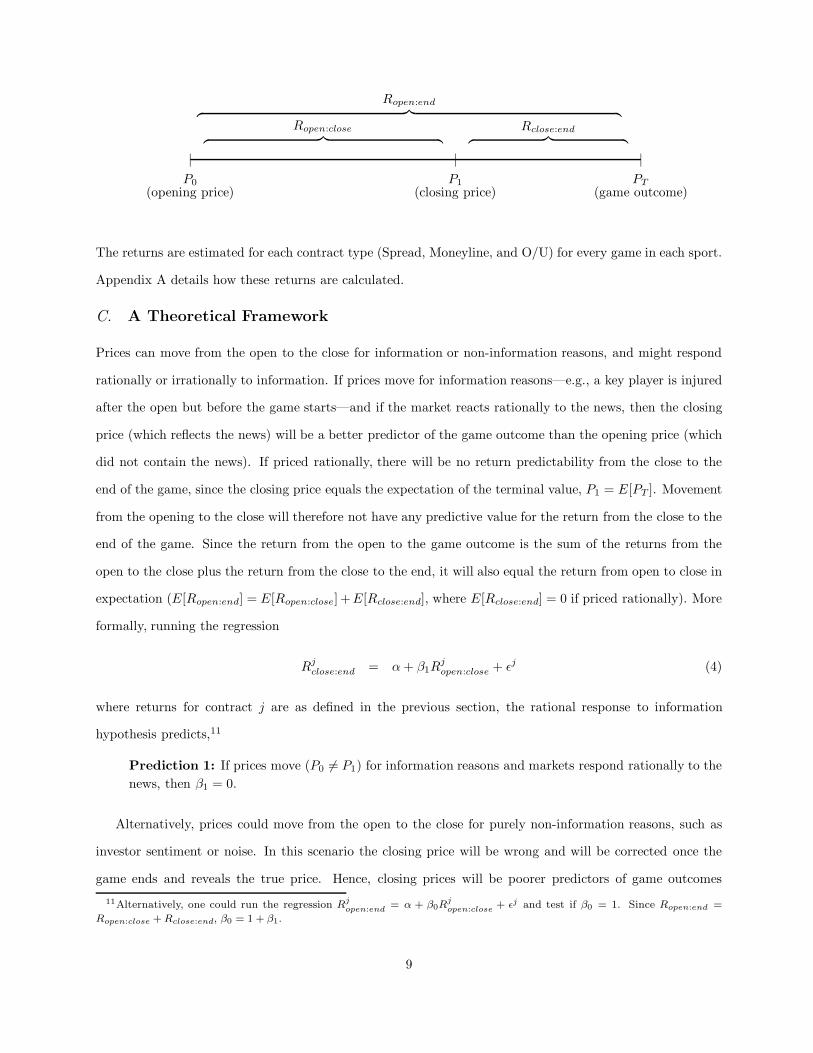
The figure below illustrates the timeline of prices I observe on each betting contract and the three periods

over which I calculate returns.10Levitt (2004) finds that NFL bookmakers predominantly do the former, though often also do the latter. They are good

at predicting betting volume and strategically take advantage of investor biases such as over-betting favorites or local teams.However, bookmakers are careful not to distort prices so much as to make a simple betting strategy, like always betting on theunderdog, become profitable.

8

Ropen:close︷ ︸︸ ︷

|

P1(closing price)

Rclose:end︷ ︸︸ ︷

PT

|

(game outcome)

Ropen:end︷ ︸︸ ︷

P0

|

(opening price)

The returns are estimated for each contract type (Spread, Moneyline, and O/U) for every game in each sport.

Appendix A details how these returns are calculated.

C. A Theoretical Framework

Prices can move from the open to the close for information or non-information reasons, and might respond

rationally or irrationally to information. If prices move for information reasons—e.g., a key player is injured

after the open but before the game starts—and if the market reacts rationally to the news, then the closing

price (which reflects the news) will be a better predictor of the game outcome than the opening price (which

did not contain the news). If priced rationally, there will be no return predictability from the close to the

end of the game, since the closing price equals the expectation of the terminal value, P1 = E[PT ]. Movement

from the opening to the close will therefore not have any predictive value for the return from the close to the

end of the game. Since the return from the open to the game outcome is the sum of the returns from the

open to the close plus the return from the close to the end, it will also equal the return from open to close in

expectation (E[Ropen:end] = E[Ropen:close] +E[Rclose:end], where E[Rclose:end] = 0 if priced rationally). More

formally, running the regression

Rjclose:end = α + β1R

jopen:close + εj (4)

where returns for contract j are as defined in the previous section, the rational response to information

hypothesis predicts,11

Prediction 1: If prices move (P0 6= P1) for information reasons and markets respond rationally to the

news, then β1 = 0.

Alternatively, prices could move from the open to the close for purely non-information reasons, such as

investor sentiment or noise. In this scenario the closing price will be wrong and will be corrected once the

game ends and reveals the true price. Hence, closing prices will be poorer predictors of game outcomes

11Alternatively, one could run the regression Rj

open:end= α + β0R

j

open:close+ εj and test if β0 = 1. Since Ropen:end =

Ropen:close + Rclose:end, β0 = 1 + β1.

9

than opening prices, implying predictability in returns from the open-to-close on final payoffs. Moreover,

the open-to-close return should negatively predict the close-to-end return as prices revert to the truth at the

terminal date, and if there was no information content in the price movement, then prices will fully revert

back to the original price at the open. Under this scenario, equation (4) predicts

Prediction 2: If prices move (P0 6= P1) for non-information reasons, then β1 = −1.

Another possibility is that prices may move for information reasons, but that the market reacts irrationally

to the news. For example, markets may underreact or overreact to the information in an injury report or

weather forecast. Indeed, under- and overreaction are two of the leading behavioral mechanisms proposed in

the asset pricing literature (Daniel, Hirshliefer, and Subrahmanyam (1998), Barberis, Shleifer, and Vishny

(1998), and Hong and Stein (1999)). In this case, closing prices would still be wrong and would therefore

imply predictability of the close-to-end return by the open-to-close return. However, the sign of this return

predictability depends on the nature of the misreaction to news on the part of investors. For example, if

markets overreact to the news, then the open-to-close return will negatively predict the close-to-end return,

but if the market underreacts to the news, then the open-to-close return will positively predict the close-to-end

return. More formally,

Prediction 3: If prices move (P0 6= P1) for information reasons but markets respond irrationally to

the news, then

(a) β1 > 0 if underreaction

(b) β1 < 0 if overreaction.

All three hypotheses—rational information, non-information, and irrational information response—make dis-

tinct predictions for the regression coefficients from equation (4).

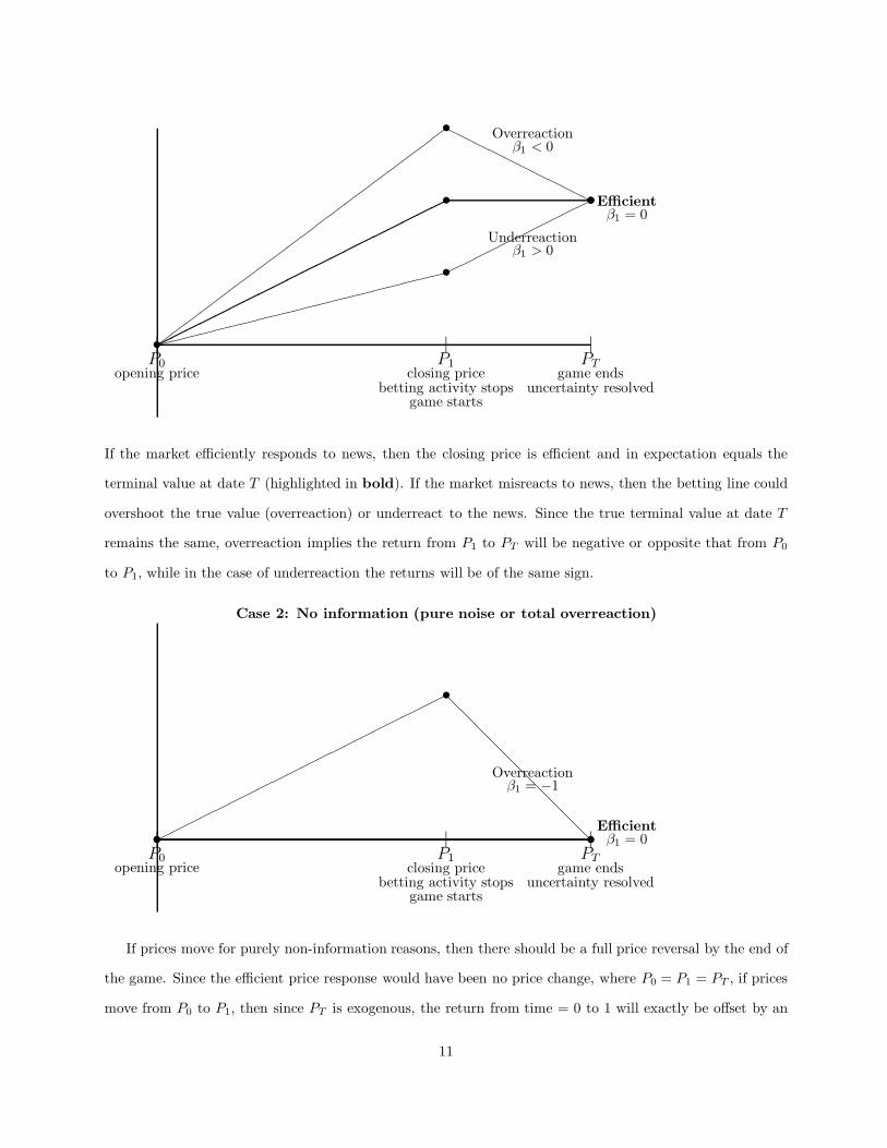
The figures below summarize the implications of Predictions 1 through 3. In the first case, assume that

the line movement contains some information, where the market can respond efficiently or inefficiently to the

news, with the latter resulting in either over- or underreaction.

Case 1: Response to news

10

•|P0

opening price

|P1

closing pricebetting activity stops

game starts

|PT

game endsuncertainty resolved

•

��

��

��

��

��

��

��

��

��

�� •Efficient

β1 = 0

•

��

��

��

��

��

��

��

��

��

��

•

HHHHHHHHHH

Overreactionβ1 < 0

•

��������������������

•

����������

Underreactionβ1 > 0

If the market efficiently responds to news, then the closing price is efficient and in expectation equals the

terminal value at date T (highlighted in bold). If the market misreacts to news, then the betting line could

overshoot the true value (overreaction) or underreact to the news. Since the true terminal value at date T

remains the same, overreaction implies the return from P1 to PT will be negative or opposite that from P0

to P1, while in the case of underreaction the returns will be of the same sign.

Case 2: No information (pure noise or total overreaction)

•|P0

opening price

|P1

closing pricebetting activity stops

game starts

|PT

game endsuncertainty resolved

• •Efficientβ1 = 0

•

��������������������

•

@@

@@

@@

@@

@@

Overreactionβ1 = −1

If prices move for purely non-information reasons, then there should be a full price reversal by the end of

the game. Since the efficient price response would have been no price change, where P0 = P1 = PT , if prices

move from P0 to P1, then since PT is exogenous, the return from time = 0 to 1 will exactly be offset by an

11

opposite signed return from time = 1 to T of equal magnitude. In this way, non-information price moves are

a special case or extreme form of overreaction.

These tests are unique to the literature and can shed light on asset pricing theory more generally. The

general idea of using differences in the ability of the opening versus final point spreads to predict game

outcomes and tease out information from sentiment effects is also explored in Gandar et al. (1988, 1998)

and Avery and Chevalier (1999), who examine the NBA and NFL, respectively. However, the tests here

are novel in several respects. First, they provide a stronger set of tests of the rational and behavioral

theories by examining return patterns over different horizons of the contract. Second, they can differentiate

among behavioral theories, namely over- versus underreaction. Third, redefining betting lines in terms of

financial returns allows for more powerful tests and more information. For example, Gandar et. al (1988,

1998) and Avery and Chevalier (1999) only look at whether closing lines are better at predicting game

outcomes, but neither paper can examine return reversals since they only look at point spreads. In addition,

couching the bets in terms of financial returns makes comparisons to capital markets easier. Finally, I link

the cross-sectional characteristics from the financial markets literature—value, momentum, and size—to the

cross-sectional return patterns in betting markets, which is unique to both literatures.

II. Data and Summary Statistics

This study examines the most comprehensive betting data to date, which includes multiple betting contracts

on the same game and across four different sports, many of which have not previously been explored in depth.

I describe the data and present summary statistics on the returns.

A. Data

Data on sports betting contracts are obtained from two sources: Covers.com (via SportsDirectInc.com) and

SportsInsights.com, two leading online betting resources.

The first data set comes from Covers.com via SportsDirect Inc. Covers.com provides a host of historical

data on sports betting markets, including betting contract prices, spreads, and outcomes, as well as historical

team and game information. The data come from many sportsbooks in both Nevada (where it is legal in the

U.S.) and outside of the U.S. and pertain only to Spread contracts for four different professional sports:

1. The National Football League (NFL) from 1985 to 2013.

2. The National Basketball Association (NBA) from 1999 to 2013.

3. The National Hockey League (NHL) from 1995 to 2013.

12

4. Major League Baseball (MLB) from 2004 to 2013.

For MLB and the NHL, Spread contracts exhibit no cross-sectional variation, merely reporting an identical

−1.5 point spread for all favorites, but where payouts adjust for the probability of winning, which is the same

as the Moneyline contract. These are also simply known as “run” lines and “puck” lines in MLB and the

NHL, respectively.

The second data set comes from SportsInsights.com and has a shorter time-series, but contains a larger

cross-section of betting contracts. The data begin in 2005 and end in May 2013 for all four sports. However,

in addition to the Spread contract, the SportsInsights data also contains information on the Moneyline and

Over/Under contracts. Opening and closing betting lines are provided on all three betting contracts for each

game. In addition, some information on betting volume (the total number of bets, not dollars) is provided

from three sportsbooks per game, which come from Pinnacle, 5Dimes, and BetCRIS who are collectively

considered the “market setting” sportsbooks that dictate pricing in the U.S. market. The betting lines are

those from the Las Vegas legalized sportsbooks and online betting sportsbooks, where all bookmakers offer

nearly identical lines on a given game.12

The data from both sources includes all games from the regular season, pre-season, and playoffs/post-

season. All games include the team names, start and end time of game, final score, and the opening and

closing betting lines across all contracts on each game. Both data sets also include a host of team and

game information and statistics, which I use in the analysis, and also supplement with information obtained

from ESPN.com, Baseball Reference.com, Basketball Reference.com, Football Reference.com, Hockey Refer-

ence.com, as well as the official sites of MLB, the NFL, the NBA, and the NHL.

For each data set, I first check duplicate games for accurate scores and remove lines that represent either

just first half, second half, or other duplicate entries that show the same teams playing on the same date

(except for a few “double headers” in MLB which had to be hand-checked). I also remove pre-season games,

all-star games, rookie-sophomore games, and any other exhibition-type game that does not count toward

the regular season record or playoffs. I then merge the two data sets and check for accuracies for the same

game contained in both data sets over the overlapping sample periods. When a discrepancy arises in final

score (which is less than 0.1% of the time), I verify by hand the actual score from a third source and use the

information from the data set that matched the third source. When a discrepancy arises in the point spread

(less than 1% of the time), I throw out that game.13

12In sports betting parlance, market setting means that other sportsbooks would “move on air” meaning that if one of thesethree big sportsbooks moved their line, other sportsbooks would follow even without taking any significant bets on the game.

13Results are robust to taking an average of the spreads or to simply using the SportsInsights spread.

13

Table I summarizes the data on sports betting contracts across the sports. Reported are the sample

periods for each sport, number of games, and total number of betting contracts. The NBA covers 18,681

games from 1999 to 2013 and 38,939 betting contracts on those games. The NFL contains 7,035 games

and 10,775 betting contracts over the period 1985 to 2013. MLB contains 23,986 games and 47,964 betting

contracts from 2005 to 2013. The NHL has 9,890 games and 19,764 betting contracts from 2005 to 2013.

Overall, the data contain 59,592 games and 117,442 betting contracts. Table I also reports the distribution

of closing lines/prices for each betting contract in each sport. The mean, standard deviation, and 1st, 10th,

25th, 50th, 75th, 90th, and 99th percentiles are reported.

B. Return Distributions

Appendix A details the construction of the sports betting contract return series. To get a sense of what these

returns look like, Figure 1 plots the time-series of aggregate sports betting returns and Figure 2 plots the

cross-sectional return distribution.

Figure 1 aggregates all of the betting returns into a portfolio by placing an equal-dollar bet in every con-

tract and every game. Specifically, every month for each contract type (Spread, Moneyline, and Over/under)

I create an equal-weighted portfolio of the betting returns on all games played that month by systematically

betting on the home team and the favored team for the Spread and Moneyline contracts, and on the over

for the Over/under contract, so that I am invested on only one side of the contract for each game. I then

compute the total return over that month across all of these bets for each contract type and across all sports.

I then equal-weight across sports. Since no sport has a season lasting a full 12 months, no month contains all

four sports with most months containing two and sometimes three sports. Repeating this every month over

the sample period I obtain a time-series of aggregate sports contract returns.

Figure 1 plots the cumulative returns to aggregate sports betting for each of the three contract types along

with the cumulative returns on the U.S. stock market (Center for Research in Security Prices value-weighted

index) over the same sample period. The sports betting aggregate returns are flat and slightly negative (due

to the vig), indicating that systematically betting on the home team, the favored team, or the over is not

profitable (i.e., that markets are efficient with respect to these attributes). More importantly, time-series

variation in the monthly sports betting returns do not appear to move at all with the stock market. The

monthly correlation between the stock market index return and the aggregate return to betting on the home,

favorite, or over is 0.06, -0.01, and 0.03, respectively, none of which are significantly different from zero.

Across all sports and games, sports betting returns appear to be independent from financial market returns,

14

which is not surprising given their idiosyncratic nature.

Turning to the cross-section of returns, which is the focus of this study, Figure 2 plots the distribution of

returns across all NBA betting contracts. Panel A shows returns to Spread contracts, Panel B to Moneyline

contracts, and Panel C to Over/under contracts. In each panel, three sets of returns are shown: open-to-

end, close-to-end, and open-to-close returns. As the figures show, within contract type, the open-to-end and

close-to-end returns have similar distributions that have a mass at −1 (losing the bet) and significant right

skewness for positive payoffs. The open-to-close returns are centered at zero since the majority of the time

the betting line does not change from the open to the close, but there is also significant variation in line

movements.

Looking across contracts, the distribution of Moneyline returns has much fatter tails than Spread or

Over/under contracts, which makes sense since Moneyline contracts have embedded leverage in them because

they adjust payoffs rather than probabilities. The Spread and Over/under contracts are very similarly

distributed. A table of summary statistics on the returns of each contract type is included at the bottom of

Figure 2. The Moneyline has the lowest mean, but fattest tails, and the Spread and Over/under contracts

are very similarly distributed with a slight negative mean for the Spread contract and a slight positive mean

for the Over/under contract, neither of which is reliably different from zero. Return distributions for the

other sports are provided in Appendix B and yield similar results.

Table II reports return correlations for each of the three betting contracts (Spread, Moneyline, and

Over/under) for each game. The non-bolded numbers in Table II are the correlations across contract types.

The correlation in returns between the Spread and Moneyline contracts is about 0.69 on average for open-to-

end and close-to-end returns, which makes sense since the Spread and ML contracts both bet on a particular

team winning, though the former contract adjusts for points while the latter adjusts the payoffs, which is why

the correlations are not one. For the O/U contracts, however, the correlation of returns with both the Spread

and ML contracts are zero at all return horizons. Essentially, the O/U contract provides an idiosyncratic

bet on the same game, which provides a set of independent return observations which can be used to test for

cross-sectional return predictability for the same game.

Within each contract type, the correlations of returns at different horizons are highlighted in bold. Not

surprisingly, the open-to-end return is very highly correlated with the close-to-end return: 0.96 for Spread,

0.99 for Moneyline, and 0.94 for O/U contracts, which simply reflects the fact that lines do not move much

between the open and the close. However, when the lines do move between open and close, the return from

open-to-close is slightly positively correlated with the open-to-end return and is negatively correlated with

15

the close-to-end return.

C. Hypothetical “Point” Returns

Since the payoffs to the betting contracts are discrete, betting outcomes may truncate useful information.

For example, suppose there are two games facing the exact same point spread of −3.5, but in one game

the favored team wins by 4 points, while in the other game the favored team wins by 20 points. In both

cases, the spread contract pays off the same amount. However, treating these two games equally throws out

potentially useful information since one team barely beat its spread, while the other exceeded its spread by a

wide margin. In order to extract more information from these betting contracts, I also compute hypothetical

returns from points scored rather than simply the discrete dollar outcomes of the contracts. Specifically, I

compute hypothetical “point” returns by replacing the dollar payoffs with the actual points scored. These

“point” returns use more information from the distribution of game outcomes and can be applied to both

Spread and O/U contracts. For Moneyline contracts the concept of point returns does not apply since those

contracts are simply bets on who wins or loses, where the payoffs have already been adjusted to reflect the

likelihood of who wins.

The correlation between the dollar returns and the hypothetical point returns is 0.79 for open-to-end

and close-to-end returns, indicating that the returns are highly correlated, but that there is also additional

information in the point returns. For the open-to-close returns, the correlation between dollar returns and

point returns is around 0.28. Results are detailed in Table A2 in Appendix A.

III. Cross-Sectional Asset Pricing Tests

I start with a general test of separating information versus sentiment-based price movements and then focus

on the three cross-sectional return predictors that have received the most attention from behavioral and

rational asset pricing—momentum, value, and size.

A. Testing General Price Movements

Before applying these tests to the cross-sectional characteristics of value, momentum, and size, I first estimate

regression equation (4) to test Predictions 1 through 3 generally in these markets. Panel A of Table III reports

results for the full sample of bets for each sport separately. The first row reports results for the NBA for

all three betting contracts, which shows a consistently strong and highly significant negative coefficient for

β1 for all three betting contracts, indicating that the close-to-end return is strongly negatively related to

16

the open-to-close price movement. These results reject Prediction 1—the rational informationally efficient

hypothesis. The regression coefficients for all three contracts are also statistically different from −1, thus

rejecting Prediction 2—the pure noise hypothesis. The results are most consistent with Prediction 3b, the

overreaction to information hypothesis. The magnitude of the coefficient, which is around −0.50 for the

Spread and Over/under contracts, suggests that about half of the total price movement from open to close

is reversed at game outcome, suggesting that the market overreacts on average by about 50 percent to price-

relevant news. For the Moneyline contract, the coefficient is −0.74, indicating a slightly stronger reversal.

The next three rows of Panel A of Table III report results for the NFL, MLB, and NHL betting contracts.

Results for the NFL Spread and Over/under contracts are very similar to those for the NBA, with negative

coefficients of −0.34 and −0.46, respectively, consistent with overreaction and rejecting both information

efficiency and pure noise. For the Moneyline contract, however, the coefficient is positive and insignificantly

different from zero, consistent with Prediction 1 and information efficiency. Anecdotal evidence from pro-

fessional sports bettors and bookmakers suggests that the Moneyline contract is dominated by professional

bettors and the least preferred by “retail” or individual/casual gamblers. Since the NFL is also the most

heavily bet sport, it is reasonable to conclude that the Moneyline contract in the NFL is relatively more

efficient than other contracts, consistent with the evidence in Table III. For MLB and the NHL, where only

Moneyline and Over/under contracts are available, the results are also similar and indicate overreaction.

Panel B of Table III repeats the regressions excluding the betting lines where there was no price movement.

The results are nearly identical, suggesting that the conditional expectation of close-to-end returns conditional

on no price movement from open to close is also zero (e.g., E[PT

P1

|P1

P0

= 0] = 0).

The results are consistent across different betting contracts and different sports, where open-to-close price

movements negatively predict close-to-end returns, consistent with overreaction. However, the question in

this paper is not whether sports betting markets in general are prone to investor sentiment, but rather

whether the same cross-sectional return predictors found in financial markets have import for sports betting

markets. For example, when lines move from open to close is it because investors chase returns by following

momentum, value, or size-related signals? And, does such movement reverse at game outcomes? Or, are

the characteristics that predict returns in financial markets unrelated to the predictability of sports betting

contract returns? I investigate these questions next.

17

B. Application to Cross-Sectional Return Characteristics

The primary goal of this paper is to investigate whether the cross-sectional characteristics of momentum,

value, and size (all defined below) are related to the return patterns above. I first examine whether movement

from the open to the close (O : C) is related to these characteristics. Specifically, I run the following regression

R̃i,O:C = αO:C + βO:CChari + ε̃i,O:C , (5)

where Chari = {Mom, Val, Size}i is the characteristic of contract i.

Following equation (4) and the logic of the previous subsection, I then regress close-to-end (C : E) returns

on the same characteristic, where the sign of the relation (if any) indicates what theories most likely explain

any relation between the characteristic and open-to-close returns. Specifically, I run the following regression

R̃i,C:E = αC:E + βC:EChari + ε̃i,C:E . (6)

In effect, the characteristic is being used as an instrument for betting line changes, where equation (5) is the

first stage and equation (6) is the second stage regression, represented here in reduced form.

There are several possible roles for the characteristics to have influence. They might affect opening

betting lines, closing lines, or movement from open to close and hence affect the return over the three

horizons considered. The pattern by which these returns are affected by the characteristic helps distinguish

among various theories, summarized by the following predictions:

1. Model 1: No Relevance. Char is not related to either information or sentiment ⇒ βO:C = βC:E = 0.

2. Model 2: Information Efficiency. Char is related to information that is priced efficiently ⇒ βO:C =

βC:E = 0.

3. Model 3: Non-information/Noise. Char is related to non-information or pure noise that erro-

neously moves prices ⇒ βO:C 6= 0, βC:E = −βO:C .

4. Model 4: Information Inefficiency/Sentiment. Char is related to information, which moves

prices (βO:C 6= 0), but the market responds inefficiently to that information. There are two types of

misreaction:

(a) Underreaction ⇒ βO:C × βC:E > 0

(b) Overreaction ⇒ βO:C × βC:E < 0.

Models 1 and 2 cannot be distinguished because both imply no relation between returns and the cross-

sectional characteristics over any horizon. Under Model 1 the characteristics either have no information value

or are not attributes bettors care about. Under Model 2 the characteristics have relevant information content,

but they are priced efficiently so that there is also no predictability in returns.

18

Models 3 and 4 are behavioral models. As Barberis and Thaler (2003) summarize, the behavioral models

deviate from rational expectations in one of two fundamental ways: differences in beliefs or differences in

preferences. Under Model 3, prices move for non-information reasons, such as preferences for a certain team

due to geographic proximity, the color jersey they play in, etc. Alternatively, it could also be the case that

investors use signals that are pure noise, erroneously believing they have information content. In either case,

if prices move for non-information reasons, prices will be inefficient and there will be predictability in returns

from the open to the close that will reverse sign from the close to the end of the game. If those non-informative

signals are related to the characteristics (momentum, value, and size) of the contracts, then those patterns

will show up in regression equations (5) and (6). Moreover, the movement in prices from open to close will

be completely reversed from the close to the game outcome, where βC:E = −βO:C . Another way to frame the

implication of this hypothesis is that the total return from open to end will be zero, despite price movement

from the open to the close, because that price movement will fully reverse at game outcome.

Model 4 is more about differences in beliefs, and is most related to the behavioral asset pricing theories

put forth to explain financial market anomalies. Under this model, the characteristics may have informa-

tion content, but the market misreacts to the information, causing mispricing. There are two possibilities:

underreaction and overreaction. Behavioral models are often motivated by, and experimental evidence from

psychology suggests, individuals underreact to mundane pieces of information and overreact to dramatic news

(see Kahenman and Tversky (1979) generally, and for references to financial applications see Barberis and

Thaler (2003)). Two of the most prominent behavioral theories for momentum and value in financial markets

focus on different aspects of information misreaction. Barberis, Shleifer, and Vishny (1998) and Hong and

Stein (1999) derive a model of underreaction to explain momentum and subsequent correction to capture

the value effect. Daniel, Hirshleifer, and Subrahmanyam (1998) have a model of delayed overreaction that

generates momentum in the short-term and eventual reversals in the long-term related to valuation ratios.

If opening and closing prices are inefficient due to misreaction that is related to the cross-sectional char-

acteristic, regression equations (5) and (6) can help distinguish between competing behavioral theories. For

example, underreaction implies that there is return predictability from open-to-close and from close-to-end

that is of consistent sign. The idea of underreaction is that markets slowly respond to the same information

and prices keep getting updated in the same direction, getting closer to the true price. This implies, for

instance, that the total return from open-to-end is greater than the return from close-to-end as the closing

price will be closer to the true efficient price.

Delayed overreaction, on the other hand, implies that prices deviate further from the truth as investors

19

continue to overreact to news. In this case, if prices are initially too high, for example, because investors

overreacted to good news, delayed overreaction will cause prices to move even higher by the close, which

implies that the return from open-to-close will be positive and the return from close-to-end will be negative.

Hence, this model implies the opposite return patterns as the underreaction model. Model 4(b) predicts

therefore that the sign of the predicted regression coefficients, βO:C and βC:E , will be opposite. In addition,

the absolute magnitude of the close-to-end return will be greater than the open-to-end return, which again

is opposite that predicted by underreaction.

Of course, a combination of effects is also possible. Opening prices may be inefficient and closing prices

efficient, or vice versa. By looking at opening price returns in conjunction with open-to-close returns and

closing price returns, I can identify whether opening or closing prices are affected differently by the same

characteristics and infer how prices are determined in this market in light of the models highlighted above.

C. Measuring Cross-Sectional Characteristics

The goal is derive cross-sectional characteristics of the sports betting contracts that are analogous to those

found in the financial markets literature. For simplicity, I focus on the NBA to illustrate the measures.

Similar measures are used for other sports.

C.1 . Momentum

The easiest characteristic to match to financial markets is momentum, since it is typically measured based

on past performance, which is also easily defined here. The literature uses the past 6 to 12 month return

on a security to measure its momentum. This is simply known as “price” momentum. Other measures of

momentum related to earnings (such as earnings surprises and earnings momentum, see Chan, Jegadeesh,

and Lakonishok (1996)) are termed “fundamental” momentum.

I construct analogous “price” and “fundamental” momentum measures for sports betting contracts using

past performance. Given the short duration of the sports contracts, the horizon relevant for momentum is

likely different than in financial markets. Theory provides little guidance on what horizon is appropriate

for momentum.14 I therefore construct a number of past return measures over various horizons, much

like Jegadeesh and Titman (1993) did in their original study. Specifically, I examine lagged measures of

performance based on: wins, point differential, dollar returns on the same team and contract type, and point

14The theoretical literature has thus far been silent on the question of horizon for momentum. Empirically, momentum isfound for past returns less than 12 months, both in the cross-section (see Jegadeesh and Titman (1993) and Asness (1994))and in the time series (see Moskowitz, Ooi, and Pedersen (2012)), with subsequent reversals occurring two to three years afterportfolio formation.

20

returns on the same team and contract type over the past 1, 2, . . ., 8 games. Eight games is roughly 10%

of the NBA season (each team plays 82 games in the regular season).

I also conduct a series of out-of-sample tests to assess the robustness of these measures and to guard

against data mining that overfits the sample. These out-of-sample tests include applying the same measures

analyzed in one sport to all other sports as well as finding measures from one time period for a given sport

and applying it to other time periods for the same sport. For example, I chose one sport—the NBA—to define

momentum measures, where I used even-numbered years to test momentum measures of various horizons,

and then examined those measures out of sample on odd-numbered years. The results were very stable along

two dimensions. First, variables that appeared stronger in even years where also shown to be stronger out of

sample in odd years. Second, and as shown below, the horizons over which momentum is measured generate

similar results. These selected measures in the NBA are then applied out of sample to other sports, where,

as will be shown, the results are also consistent.

The first two momentum measures are at the team level and the last two measures are at the contract

level (Spread, Moneyline, O/U), with the former being “fundamental” momentum and the latter “price”

momentum.15 In addition, I also create a momentum index of all these measures by taking a principal

component-weighted average of the momentum measures from their correlation matrix (since the variables

are in different units and scales).

Since every game is a contest between two teams, the momentum measure for the betting contract is

the difference between the team momentum measures. For example, the momentum measure on a Spread

contract bet on team A versus team B using past dollar returns over the last N games is,

MOM$ret,Nt (A vs. B) =

N∑

g=1

RS,$t−g,close:end(A) −

N∑

g=1

RS,$t−g,close:end(B), (7)

where RS,$t−g(A) is the dollar return from betting on team A in a Spread contract in the most recent gth

game that team A has played prior to time t. Equation (7) can be easily estimated for other momentum

measures by substituting point returns, wins, or point differentials in place of the past dollar returns. In

addition, equation (7) can be estimated for other sports betting contracts such as the Moneyline, where the

past Spread contract returns are replaced with the past Moneyline contract returns.

For Over/under contracts, which is a bet on the total number of points scored rather then who wins and

by how much, I take the sum of the team momentum measures rather than their difference. However, since

15All lagged measures within a season only pertain to games within that season. I do not use games from the previous seasonto construct past game performance measures since there is a significant time lag between seasons where teams can change alot. Hence, for the NBA, the first set of betting contracts each season starts with game nine when looking at eight game laggedmeasures.

21

the O/U contract is a bet on total points scored and not who wins, I expect the results using past wins to

be much weaker here than for the Spread and ML contracts—a conjecture I test in the next section.

Panel A of Table IV reports the correlations of the various momentum variables across games for different

lags. The measures are all highly correlated, with the “fundamental” team-level momentum measures (win

percentage and net points) having a 0.81–0.88 correlation with each other, the “price” contract-level momen-

tum measuures (dollar and point returns) having a 0.78–0.79 correlation to each other, and the correlation

between fundamental and price momentum being around 0.65.16 The last row of Panel A of Table IV re-

ports the correlation of the momentum principal component index (Mom PC) with each group of momentum

measures averaged across all lags. The Mom PC index is highly correlated with each momentum measure.

C.2 . Value

A more difficult characteristic to match to financial markets is value. In equities, value is often measured

by the ratio of book value of equity to market value of equity or some other ratio of “fundamental” value to

market value of the firm (e.g., E/P, D/P, CF/P; see Fama and French (1992, 1993, 1996, 2012), Lakonishok,

Shleifer, and Vishny (1994), and Israel and Moskowitz (2013), among others.) Another value measure used

that is highly correlated with fundamental-to-market value ratios is the negative of the long-term past return

on the asset, following DeBondt and Thaler (1985, 1987), Fama and French (1996), and more recently Asness,

Moskowitz, and Pedersen (2013), who find that long-short equity strategies sorted on the negative of past

three year returns are 0.86 correlated to strategies formed on book-to-market equity in both the U.S. and

globally across a dozen developed equity markets.

As with momentum, I construct a number of value measures motivated by the finance literature. I group

them into three categories: long-term past performance, fundamental-to-price ratios, and residual measures.

1. Long-term past performance. Following DeBondt and Thaler (1985, 1987), Fama and French

(1996), and Asness, Moskowitz, and Pedersen (2013), I use measures of past performance over the

previous one, two, and three seasons to capture value.

2. Fundamental-to-market ratios. Following Fama and French (1992, 1993, 1996, 2012) and Lakon-

ishok, Shleifer, and Vishny (1994), I take various book values of the team franchise, including book

value of the team, ticket revenue, total revenue (gate sales plus souvenir sales, TV rights, concessions,

etc.), and player payroll, and divide each by the current spread on the Spread contract.

The idea is to use some measure of the “book value” of the underlying team and scale that by the

current market price, in this case the spread, on the game itself. For example, differences in player

payroll between the two teams divided by the spread seems to capture the notion of value used in

16These correlations among different momentum measures are actually very similar to those used in financial markets, where,for instance, Chan, Jegadeesh, and Lakonishok (1996) find that price and earnings momentum are about 0.60 correlated.

22

financial markets. If the labor market for athletic talent is somewhat efficient, then two teams facing

different payrolls should in principal face different probabilities of winning the game. However, payroll

is a slow-moving long-term measure of value/team quality. The spread, on the other hand, provides the

market’s current assessment of how likely the team will win and by how much. Hence, a game that has

big differences in payroll and little differences in spread (or opposite signed differences in the spread),

will look “cheap,” or a value bet.

Another measure of value following the same theme is to come up with a fundamental value of the

game itself. Luckily, the sports analytics community has derived a number of measures of team quality

or strength for use in predicting wins. The most popular is known as the Pythagorean win expectation

formula. Appendix C provides details and intuition for this formula, which has been applied to all

sports. The formula provides an expected win percentage for each team, which I use as a relative

strength measure by taking the difference between the measures for each team and then dividing that

difference by the current betting line or contract price, E(P )/P .

3. Residual measures. Finally, another way to measure value is to directly try to identify surprisingly

cheap or expensive looking contracts. For example, calculate the expected Spread (or Moneyline or

O/U total) on a contract based on observable information and use deviations of the actual Spread from

its expectation as a value indicator. Contracts with positive residuals are expensive and those with

negative residuals are cheap relative to observable information.

I also take a principal component-weighted average of the value measures within each group and across

all groups from their correlation matrix.

Panel B of Table IV reports the correlations across the various value measures. The long-term past

return measures are pretty highly correlated with each other, as are the fundamental-to-price ratios, with

correlations ranging from 0.52 to 0.97. However, the correlations between the long-term performance measures

and the fundamental ratio measures are close to zero. The principal component-weighted index for value has

correlations of -0.30, -032, -0.30 with the long-term past performance (dollar returns) of betting on the same

team over the last season, two seasons, and three seasons, respectively. The correlation of the value index to

the fundamental-to-price ratios are 0.43, 0.45, 0.46, and 0.50. These correlations are very much consistent

with what is found in financial market data, where the long-term past performance on an asset is a negative

indicator of its value and negatively correlated to fundamental-to-price ratios. (For equities in the U.S., the

average correlation between long-term past returns and book-to-market equity ratios is -0.40.) The ratio of

predicted or expected contract price relative to actual price, E(P )/P , is negatively related to the long-term

past performance measures and positively related to the fundamental-to-price measures, consistent with it

being a good proxy for value. Its correlation to the value index is 0.56. The regression residual is basically

uncorrelated to any of the other value measures, which is not terribly surprising since it controls for long-term

observable variables (which the other value measures are based on) and hence largely captures short-term or

unobservable information related to deviations in price.

23

The value measure for each game is the difference between the team value measures for the Spread and

Moneyline contracts and the sum of the two measures for the Over/under contracts.

C.3 . Size

To measure size, I simply use annual franchise value, ticket revenue, total revenue, and player payroll. These

measures are highly correlated with the size of the local market in which the team resides as well as the

popularity of the team, which is a function of many things including long-term historical performance. These

are very slow moving variables whose cross-sectional ranking does not change much over time (e.g., the New

York teams are always “larger” than the teams in Pittsburgh). Panel C of Table IV shows that the size

measures are all highly correlated with each other.

Finally, Panel D of Table IV reports the correlations of the momentum, value, and size indices. Consistent

with the measures used in financial markets, the value and momentum measures are negatively correlated,

albeit not as strongly as they are in financial markets (see Asness, Moskowitz, and Pedersen (2013)), and

so are the size and value measures (see Fama and French (1992, 1993)). Size and momentum are slightly

positively correlated. Hence, the correlations across characteristics are also consistent with those used in

financial markets.

C.4 . Cross-validation

While it is nearly impossible to get consensus on what the right momentum, value, and size measures are,

and this is true in general, the above measures seem to reasonably match the variables examined in financial

markets. Moreover, as emphasized earlier, none of these measures were selected to match returns in this

market, but rather are motivated by similar measures that have been shown to explain returns in financial

markets. In addition, the use of many measures allows for an assessment of the robustness of the results and

using an average across measures helps reduce noise (see Israel and Moskowitz (2013)). Additionally, the

many out-of-sample tests performed in this study should alleviate any data mining or overfitting concerns.

I also asked two of the leading scholars from both sides of the efficient markets debate: Eugene Fama

(proponent of the rational risk-based view and winner of the 2013 Nobel Prize in Economic Sciences in part for

his work on efficient markets) and Richard Thaler (pioneer of behavioral finance and the current co-director,

along with Robert Shiller 2013 Nobel recipient, of the Behavioral Finance working group at the NBER) to

weigh in on the plausibility of these measures before they or I saw any of the results.17 The following are

17This way nobody could complain ex post about the measures if the results failed to confirm their priors.

24

quotes from each when asked whether they thought these were reasonable measures of momentum, value,

and size analogous to those used in financial markets:

Fama: “Most of these make sense to me. . . . I like past team record longer-term for value,

shorter-term for momentum. But the rest seemed ok.”

Thaler: “Momentum is easier. For value, since that’s my [referring to long-term past perfor-

mance] measure with DeBondt, I guess I have to like that one. I also like the difference in power

rankings or quality divided by contract price as a measure of what behavioralists think of value.”

D. Momentum

Armed with these measures for every game, I test whether high versus low exposure to each characteristic

predicts future returns on average. I begin by reporting a full set of results for the NBA, and then report an

abbreviated set of results for the other sports for brevity and simplicity.

Table V reports results from estimating equations (5) and (6) by regressing the returns from open-to-close

and close-to-end, respectively, on the various momentum measures described above.18 The first row of Panel

A of Table V reports results for the open-to-close returns of Spread contracts. For the point differential

momentum measures, there is a strong positive relation between momentum and the open-to-close return

at a one game lag, and a weakly positive relation between momentum and returns at 4 and 8 game lags,

with similar sized coefficients. Using the past dollar return momentum measures, there is an even stronger

positive relation with open-to-close returns at all game lags, with the strongest being at a one game lag.

These results indicate that movement in the betting line from the open to the close is positively related to

recent past performance, consistent with momentum, and where fundamental and price momentum measures

yield similar results. The last column reports results for the momentum index, which shows a positive and

significant coefficient (t-statistic = 2.34).

The second row of Panel A of Table V reports results for close-to-end returns on the momentum measures.

Here, the coefficients are predominantly negative, and marginally significant for the most recent past dollar

returns. These results indicate a reversal of the momentum effect that moved prices from the open to the

close. Following Section D.A, this result is consistent with a model of overreaction for momentum, where

investors push prices too far from the open to the close based on past performance that then reverses at the

game outcome. The third row reports whether the reversal from close to end fully captures the movement

18The win percentage and point differential momentum measures are highly correlated and yield similar results, hence forbrevity, I only report the point differential measures.

25

from open-to-close. Specifically, a formal test of whether βO:C,Mom = −βC:E,Mom is performed. As Table

V indicates, I fail to reject the hypothesis that the betas have opposite sign but identical magnitudes. This

indicates that I cannot reject that a full reversal of the opening to closing price movement from momentum

occurred.

The evidence supports a partial efficiency story of overreaction, where opening prices seem to be set

efficiently with respect to past performance, but prices seem to move from the open to the close based on

investors chasing past performance that pushes prices too high based on good past performance and too low

based on poor past performance. As a consequence, there is positive momentum based on past performance

from the open to the close, and a full reversal from the close to the game outcome when the true terminal

value is revealed. These patterns are consistent with the delayed overreaction story for momentum of Daniel,

Hirshleifer, and Subrahmanyam (1998).

The next three rows of Panel A repeat the regressions using hypothetical “point” returns instead of dollar

returns, where the point returns, as argued above, may capture more information since their payoffs are

not truncated. The results using point returns are stronger and match directionally the results using dollar

returns: momentum has strong positive predictability for open-to-close returns that reverses for close-to-end

returns. These results are consistent with an overreaction story for momentum.

Panel B of Table V repeats the same regressions for the Moneyline contracts. For Moneyline contracts,

only dollar returns are available. The results are mixed. For the point differential momentum measures,

there is positive predictability from open-to-close and close-to-end and the strength of the relationship seems

to increase with the length of the lag of past performance. However, using the dollar return momentum

measures, the results are more consistent with Panel A, where there is positive predictability from open-

to-close and a reversal from close-to-end, consistent with overreaction, though the effects are not generally

significant. It is possible that the Moneyline contract, which is more popular among professional bettors,

may be less prone to momentum patterns. These results are interesting because the Spread and Moneyline

contract payoffs are 0.69 correlated, yet the momentum returns in the Spread contract do not show up as

strongly in the Moneyline contract.

Panel C of Table V looks at the same regression results for the Over/under contracts, which, like the

Spread contract, are more popular among casual bettors. Recall, that the returns of the Over/under contract

are uncorrelated with those on the Spread contract (see Table II). However, despite this zero correlation on

average, the results for momentum on Over/under contracts are very consistent with those for the Spread

contract in Panel A. There is strong positive predictability from momentum on open-to-close returns, with a

26

significant reversal from close-to-end that appears to fully reverse the opening price movement, consistent with

the overreaction hypothesis. The results are stronger using the point (fundamental) momentum measures

rather than the past dollar return (price) measures, which makes sense because the Over/under contract is a

bet on total points scored and hence point totals may be more salient and relevant to investors. In addition,

while past win percentage, which is highly correlated with point totals, delivers positive momentum for the

Spread and Moneyline contracts, which are bets on who wins, it does not predict Over/under returns well,

which is also consistent with this conjecture.

Overall, Table V provides evidence across three different betting contracts consistent with a delayed

overreaction story for momentum. The results suggest that opening prices are on average efficient with

respect to past performance, but investors chasing performance push prices too far in the same direction by

the close, resulting in positive momentum from open-to-close that subsequently reverses from close-to-end

when uncertainty is resolved.

Table VI reports results on momentum for the other sports, estimated separately for the NFL (Panel A),

MLB (Panel B), and the NHL (Panel C), where there are no Spread contracts for MLB and the NHL. The

results are consistent with those for the NBA in Table V. Finding the same pattern in three other distinct

sports and in three betting contract types using the same momentum measures provides an impressive set

of out-of-sample evidence alleviating data mining concerns, especially considering that the contracts across

sports are independent.

While the coefficients are of consistent sign, their statistical significance is sometimes lacking, which could

be due to low power. To increase the power of the tests, Panel D of Table VI reestimates the regressions using

all four sports (including the NBA) simultaneously. The results show a statistically strong and significant

positive momentum pattern from open to close and then an equally strong reversal from close to end. The

t-statistics on the positive momentum coefficients from open to close are all large and significant, ranging

from 3.66 to 10.19, and the negative reversals from close to end exhibit significant t-statistics ranging from

−2.33 to −2.97.

Figure 3 summarizes the results across all four sports by plotting the t-statistics of the betas on momentum

(using the average across all momentum measures) over each return horizon, for each betting contract type,

in each sport. The regressions are estimated for each momentum measure from Section III individually and

then the t-statistics from these regressions are aggregated across all momentum measures and plotted over

each return horizon for each sport separately in Panels A–D as well as for the NBA and NFL combined (Panel

E) and across all four sports (Panel F) combined.

27

A consistent pattern emerges for the Spread and Over/under contracts in every sport, where the momen-

tum betas exhibit a tent-like shape over the three horizons—near zero from open-to-end, significantly positive

from open-to-close, and significantly negative from close-to-end, with the initial price movement from open-

to-close related to momentum being fully reversed by the game outcome. The patterns for the Moneyline

contracts exhibit the same tent-like shape, but are less pronounced, consistent with the Moneyline perhaps

being less affected by “dumb” money and more dominated by “smart” money.19

E. Value

Table VII reports regression results from estimating equations (5) and (6) for the value measures for the

NBA only. Panel A contains the results for Spread contracts, and Panels B and C report results for the

Moneyline and Over/under contracts. Each value measure is signed so that it can be interpreted as a

measure of cheapness (i.e., negative of past performance, negative of residual) and in this way have the

opposite expected sign as the momentum variables.

The first row of Panel A of Table VII reports the value regression results for open-to-close returns. Almost

all of the coefficients on the value measures are negative. The second row reports results for close-to-end

returns, where the coefficients on value are predominantly positive. Cheap contracts get cheaper between

the open and close, and the positive returns from close to end indicate that part of this price movement

is inefficient. These patterns are consistent with the delayed overreaction story of Daniel, Hirshleifer, and

Subrahmanyam (1998) for value, where investors overreact to news that generates a negative relation between

future returns and fundamental-to-price ratios or negative long-term past returns. However, most of the

coefficients are not reliably different from zero, save for the past one and two seasons of contract return

performance.

The point estimates from the regression are generally consistent with an overreaction story related to

value, but the results are statistically weak. A generous interpretation emphasizes that the point estimates

tell a consistent story that matches the story from the momentum results, and the lack of significance could

be due to low power and the difficulty and noise in measuring value. A less generous interpretation argues

19I also interacted the momentum measures with measures of investor salience—a feature that stands out or captures the focusof investors who may face limited attention (Barber and Odean (2008)). I create a dummy variable which identifies a rare orextreme event that fans and the media may pay extra attention to: a player in the NBA scoring at least 50 points in the mostrecent game or recent eight games (only 104 occurrences in the 18,681 games I examine), “triple doubles,” team total pointsgreater than 140, all of which yielded similar results. For other sports I use salience measures in the same spirit, such as threeor more touchdowns by any player in the NFL, a “hat trick,” which is three goals or more in hockey, and multiple home runsby any player in MLB. Table B3 in the appendix reports the results, which for brevity, are only reported for the momentumindex for both dollar and point returns. As the table shows, the interaction terms between momentum and saliency have thepredicted sign but are statistically insignificant.

28

that value may have no predictive content in this market either because it is related to systematic risk, which

is absent in this market, or because value is a much slower moving variable than momentum and the market

is therefore better able to price it.

To help address the power issue, the bottom two rows of Panel A of Table VII repeat the regressions using

the hypothetical point returns, which may contain more information. Here, there is similar and stronger pre-

dictability for value on the returns from the open to the close, and in a direction consistent with overreaction.

The close-to-end returns associated with value are positive, which is also consistent with a correction of the

market’s overreaction.

Estimating the regressions for the Moneyline (Panel B) and Over/under (Panel C) contracts, I get very

similar results: consistently negative coefficients on value measures from open-to-close and positive coefficients

from close-to-end, all of which are supportive of an overreaction story, but the evidence is statistically weak.

Table VIII reports results for the value regressions among the other sports. Just the composite value index

is used for brevity for both dollar and points-based returns as the dependent variable in the regressions. The

results are very consistent with those shown above for the NBA. To increase the power of the tests, Panel

D of Table VIII repeats the regression for all sports (NBA, NFL, MLB, and NHL). The results show a

statistically strong negative coefficient on value for open-to-close returns, consistent with an overreaction

story and consistent with the increased power of the tests coming from combining all sports. However, the

coefficients from open to end remain insignificant, though positive, consistent with price correction from

initial overreaction.

Figure 4 summarizes the results for value across all four sports by plotting the average t-statistics of

the value betas estimated for open-to-end, open-to-close, and close-to-end returns for each betting contract

type. A consistent pattern is evident from the plots: a value contract’s betting line declines between the

open and close and then rebounds between the close and game end, reaching the same level it started at

the open. These patterns are consistent with an overreaction story for value, where value contracts, which

measure “cheapness”, continue to get cheaper between the open and the close, becoming too cheap and thus

rebounding positively when the game ends. This picture is the mirror image of momentum, where value or

cheapness is negatively related to past performance, and hence the pictures for momentum and value tell the

same story. (Though, recall the measures for value and momentum were only mildly negatively correlated.)

29

F. Size

Table IX reports results for regressions on size. Here, there is no predictability of any kind—statistically,

economically, or even of consistent sign—for any contract over any horizon, regardless of the size measure

used. Size, which is the slowest moving of all the variables examined, seems to be either efficiently priced in

both opening and closing prices, or is irrelevant to sports bettors. Table X repeats the size regressions for

the other sports and similarly finds nothing.

Table B4 in the appendix reports results for multivariate regressions that use momentum, value, and size

simultaneously in the regressions. Here, I use the composites of momentum, value, and size for brevity. The

results are largely consistent with the univarirate regressions for each characteristic.

IV. Comparison to Financial Markets

Given the existence of momentum and value return premia in these idiosyncratic sports betting contracts,

a natural question arises as to how to compare these returns to analogous momentum and value returns in

financial markets? In addition, since the return patterns are consistent with investor overreaction, does this

help shed light on these patterns in financial markets?

A. Trading Strategy Profits and Costs

To compare the economic significance of the predictability of returns in sports betting markets to financial

markets, Table XI reports trading strategy profits from using momentum, value, and size in both markets.

A.1 . Sports Betting Trading Strategies

Using the composite measures for momentum, value, and size, a trading strategy is formed that invests

positively (for the favorite) when predicted movements in the betting line are expected to be positive (i.e.,

continuation) and invests negatively (takes the other side of the bet) when line movements are predicted to

be negative (i.e., reversals), where the dollars bet are in proportion to how strong the signal or characteristic

predicting price movement is relative to the cross-sectional average. Specifically, the average trading strategy

returns are computed as follows:

R̄p,t =1

T

T∑

t=1

φt

N∑

j=1

(Charij,t −

1

N

N∑

j=1

Charij,t)r̃

ij,t ∀i ∈ (S, ML, O/U) (8)

where Char = {momentum, value, size} are signed to predict returns positively (hence, momentum and value

enter with opposite sign to predict returns) for game j. For Spread and Moneyline contracts, a positive weight

30

means betting for the favored team and a negative weight means betting on the underdog. For Over/under

contracts a positive weight means betting on the over and a negative weight means betting on the under.

The total bets summed across all games are rescaled to add up to one dollar at each point in time, which

is what the scalar φt does.20 All bets across all contracts are aggregated monthly. Results are reported

separately for each characteristic by itself as well as a combination of all three characteristics used to predict

line movements called “multi-strategy”. Trading strategy profits are computed for both open-to-close returns

and for close-to-end returns.

Two average returns are computed: 1) gross returns and 2) net returns that account for transactions

costs (the “vig”). The gross Sharpe ratio of the strategy is also reported. All returns and Sharpe ratios are

reported as annualized numbers. Panel A reports results for the NBA only and Panel B reports results by

combining all of the bets across all four sports into one portfolio, where each sport is given equal weight in

the portfolio.

The first column of Panel A of Table XI reports that annualized gross returns to betting on momentum,

value, and size for open-to-close returns in the NBA are 60, 21, and −26 basis points, respectively. The

positive predictability in returns from momentum and value is consistent with the previous findings from

the regressions. The multi-strategy portfolio that combines all three characteristics yields 64 basis points on

average per year. The second set of four rows report the gross returns from close to end (where I reverse the

sign so that all trading strategies in expectation will yield positive returns). Here, momentum produces 52

basis points and value 156 basis points, with the multi-strategy yielding 256 basis points.

While the gross returns are positive (except size), the net returns reported in the second column are

significantly negative because of the vig, which at 10 percent on average easily wipes out any profits from

momentum and value, especially for open-to-close returns, since the vig is incurred twice (once at the open

and then again at the close when unwinding the position). The third column reports the gross Sharpe ratio

of each strategy, which ranges from −0.04 for size to 0.10 for the multi-strategy.

Panel B of Table XI reports trading strategy profits using bets across all four sports. While the gross

returns are pretty similar in magnitude to those from the NBA, the net returns and Sharpe ratios are

typically bigger due to lower volatility from increased diversification of using many more uncorrelated bets

across four different sports. Once again, however, none of these strategies are able to overcome trading

costs. Given the size of the vig, attempting to arbitrage away the predictability of returns coming from

momentum and value would prove unprofitable, and hence justifies why such predictability remains in the

20Similar results are obtained assuming $1 is bet equally across all contracts.

31

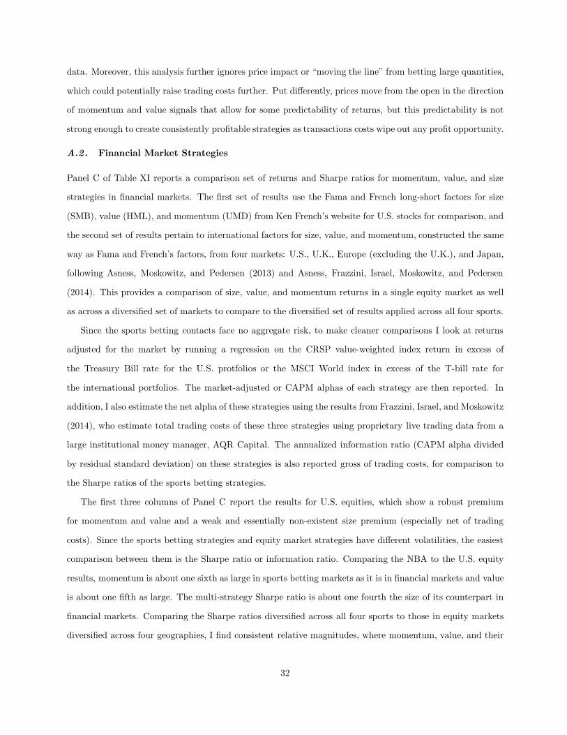
data. Moreover, this analysis further ignores price impact or “moving the line” from betting large quantities,

which could potentially raise trading costs further. Put differently, prices move from the open in the direction

of momentum and value signals that allow for some predictability of returns, but this predictability is not

strong enough to create consistently profitable strategies as transactions costs wipe out any profit opportunity.

A.2 . Financial Market Strategies

Panel C of Table XI reports a comparison set of returns and Sharpe ratios for momentum, value, and size

strategies in financial markets. The first set of results use the Fama and French long-short factors for size

(SMB), value (HML), and momentum (UMD) from Ken French’s website for U.S. stocks for comparison, and

the second set of results pertain to international factors for size, value, and momentum, constructed the same

way as Fama and French’s factors, from four markets: U.S., U.K., Europe (excluding the U.K.), and Japan,

following Asness, Moskowitz, and Pedersen (2013) and Asness, Frazzini, Israel, Moskowitz, and Pedersen

(2014). This provides a comparison of size, value, and momentum returns in a single equity market as well

as across a diversified set of markets to compare to the diversified set of results applied across all four sports.

Since the sports betting contacts face no aggregate risk, to make cleaner comparisons I look at returns

adjusted for the market by running a regression on the CRSP value-weighted index return in excess of

the Treasury Bill rate for the U.S. protfolios or the MSCI World index in excess of the T-bill rate for

the international portfolios. The market-adjusted or CAPM alphas of each strategy are then reported. In

addition, I also estimate the net alpha of these strategies using the results from Frazzini, Israel, and Moskowitz

(2014), who estimate total trading costs of these three strategies using proprietary live trading data from a

large institutional money manager, AQR Capital. The annualized information ratio (CAPM alpha divided

by residual standard deviation) on these strategies is also reported gross of trading costs, for comparison to

the Sharpe ratios of the sports betting strategies.

The first three columns of Panel C report the results for U.S. equities, which show a robust premium

for momentum and value and a weak and essentially non-existent size premium (especially net of trading

costs). Since the sports betting strategies and equity market strategies have different volatilities, the easiest

comparison between them is the Sharpe ratio or information ratio. Comparing the NBA to the U.S. equity

results, momentum is about one sixth as large in sports betting markets as it is in financial markets and value

is about one fifth as large. The multi-strategy Sharpe ratio is about one fourth the size of its counterpart in

financial markets. Comparing the Sharpe ratios diversified across all four sports to those in equity markets

diversified across four geographies, I find consistent relative magnitudes, where momentum, value, and their

32

combination generate return premia per unit of risk about one fifth the size of those in financial markets.

Given these magnitudes, an interpretation of the data is that momentum and value effects, that are not

coming from a systematic source of risk, produce returns per unit of risk about one fifth as large as what

we observe in financial markets. From a behavioral view, one might argue that this evidence suggests that

a significant, or at least non-trivial, portion of momentum and value patterns in markets could be coming

from non-systematic sources, possibly related to investor behavior and sentiment. On the other hand, from a

rational risk-based view, the magnitude of the premia generated from these non-systematic sources is small

compared to the premia in financial markets, and hence the behavioral theories may only contribute a small

part to these premia. Furthermore, given the large trading costs in sports markets, the magnitude of these

effects may be even smaller in financial markets if arbitrage activity is less limited.

B. Covariance Structure

Another key piece of evidence from financial markets on momentum and value (and size) returns is that there

is significant covariance structure in the returns to these strategies (e.g., Fama and French (1993, 1996),

Carhart (1997), Asness, Moskowitz, and Pedersen (2013), Lewellen, Nagel, and Shanken (2009) and Daniel

and Titman (2010)). The significant covariance structure among these portfolios has often been interpreted

as consistent with underlying common risk factors driving their returns. Behavioral models do not explicitly

have a role for comovement and indeed this is one of the distinguishing features that Daniel and Titman

(1997) try to exploit in testing rational versus behavioral theories. On the other hand, more recent models

of investor behavior and institutional frictions derive a role for covariation among these portfolios through

herding and benchmarking (e.g., Barberis and Shleifer (2004)) or correlated behavior and rebalancing (e.g.,

Vayanos and Wooley (2012)).

Given the idiosyncratic nature of the sports betting contracts, it is interesting to examine whether there is

any covariance structure among portfolios of these contracts sorted by the same characteristics. If covariance

structure exists in these markets, it cannot be driven by aggregate risk sources and hence must come from

other sources such as correlated investor behavior. If, however, no such comovement is present in these

markets, then this could possibly be consistent with the common risk factor interpretation given to the

comovement witnessed in financial markets.

Table XII reports regression results of portfolios of contracts formed on momentum and value and regressed

on a momentum and value “factor,” similar in spirit to what has been done in the financial markets literature.

The test portfolios are formed by sorting all games in a given month (with at least 40 games) by their

33

momentum (value) characteristic, which is the weighted-average index, into five quintiles and then taking the

equal-weighted average return of all games within each group. This provides a monthly return to quintile

sorted portfolios based on momentum (value), whose returns are then regressed on the monthly returns of

the momentum (value) factor, which is the high minus low quintile spread returns, Q5 − Q1.

Panel A of Table XII reports results for test assets and factors formed from the same games such that

there is overlap of the betting contracts that comprise the test portfolios and the factors. Panel B of Table

XII reports results for the same exercise where the test assets and factors are formed from non-overlapping

games—e.g., one set of games is used to form the test assets and another set of games is used to form the

factors. To compute the test portfolios and the factors independently each month the number of games are

split randomly into two groups, with one used to form the test assets and the other used to form the factors,

with no overlap in contracts on the left and right hand side of the regression. Reported are the coefficient

estimates (β) on the factor, its t-statistic in parentheses, and the R2 from each regression. The intercept is

not reported for brevity.

Panel A, which reports results for the overlapping sample, shows strong covariation for the extreme

portfolios (the low and high quintiles), but no covariation for quintiles 2 through 4. The covariation with

the extreme portfolios are simply mechanical in that the factor itself is comprised of the same games that

enter the extreme quintile portfolios. The lack of significance of any betas and the low R2s for quintiles 2

through 4 indicate that there is no covariance structure present once this mechanical relation is no longer

present. Confirming this conclusion, Panel B shows that there is no covariance structure at all across any of

the quintiles, including the two extremes, when the test assets and factors contain non-overlapping games.

Hence, there appears to be no significant covariance structure to either momentum or value-sorted portfolios

among the sports betting contracts. The difference in results between Panels A and B highlights the dangers

in using overlapping securities on both the left and right hand sides of the regression in conducting these tests

generally. The lack of covariance structure is consistent with a behavioral interpretation of the momentum

and value premia in these markets and is in contrast to the significant covariance structure found in financial

markets for momentum and value strategies.21

C. From Sports to Financial Markets: A Further Test of Overreaction

To establish an even tighter link between sports and financial markets for learning about asset pricing, I

derive an additional insight from sports betting prices that I then test in financial markets. Specifically, since

21I also examined whether there was any covariation in value or momentum sorted portfolios across sports. Not surprisingly,since there is no correlation within a sport, there was also no correlation across sports in terms of the portfolios’ returns.

34

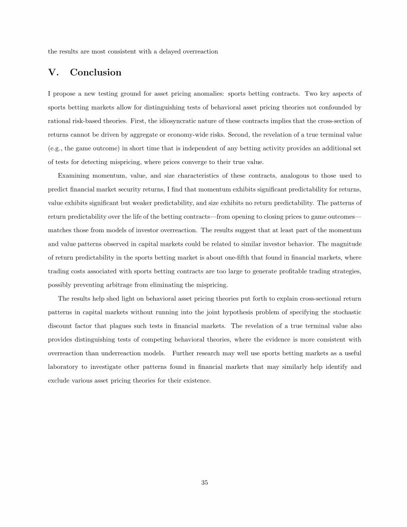
the results are most consistent with a delayed overreaction

V. Conclusion

I propose a new testing ground for asset pricing anomalies: sports betting contracts. Two key aspects of

sports betting markets allow for distinguishing tests of behavioral asset pricing theories not confounded by

rational risk-based theories. First, the idiosyncratic nature of these contracts implies that the cross-section of

returns cannot be driven by aggregate or economy-wide risks. Second, the revelation of a true terminal value

(e.g., the game outcome) in short time that is independent of any betting activity provides an additional set

of tests for detecting mispricing, where prices converge to their true value.

Examining momentum, value, and size characteristics of these contracts, analogous to those used to

predict financial market security returns, I find that momentum exhibits significant predictability for returns,

value exhibits significant but weaker predictability, and size exhibits no return predictability. The patterns of

return predictability over the life of the betting contracts—from opening to closing prices to game outcomes—

matches those from models of investor overreaction. The results suggest that at least part of the momentum

and value patterns observed in capital markets could be related to similar investor behavior. The magnitude

of return predictability in the sports betting market is about one-fifth that found in financial markets, where

trading costs associated with sports betting contracts are too large to generate profitable trading strategies,

possibly preventing arbitrage from eliminating the mispricing.

The results help shed light on behavioral asset pricing theories put forth to explain cross-sectional return

patterns in capital markets without running into the joint hypothesis problem of specifying the stochastic

discount factor that plagues such tests in financial markets. The revelation of a true terminal value also

provides distinguishing tests of competing behavioral theories, where the evidence is more consistent with

overreaction than underreaction models. Further research may well use sports betting markets as a useful

laboratory to investigate other patterns found in financial markets that may similarly help identify and

exclude various asset pricing theories for their existence.

35

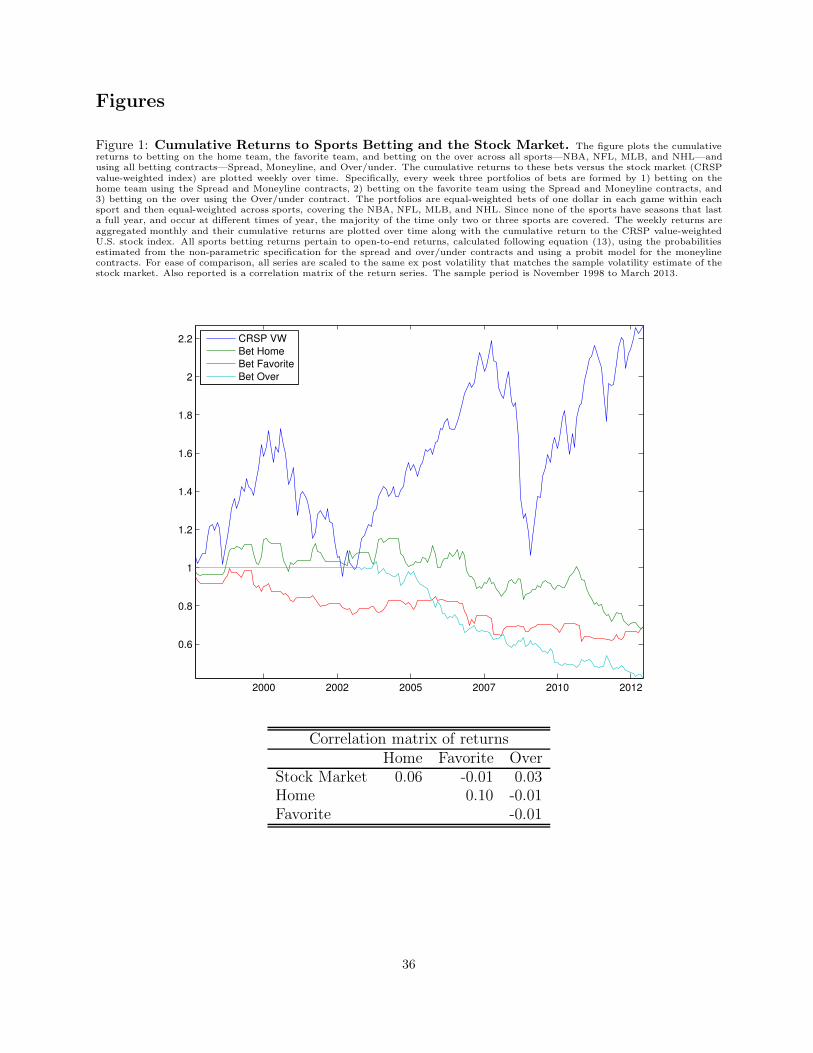
Figures

Figure 1: Cumulative Returns to Sports Betting and the Stock Market. The figure plots the cumulativereturns to betting on the home team, the favorite team, and betting on the over across all sports—NBA, NFL, MLB, and NHL—andusing all betting contracts—Spread, Moneyline, and Over/under. The cumulative returns to these bets versus the stock market (CRSPvalue-weighted index) are plotted weekly over time. Specifically, every week three portfolios of bets are formed by 1) betting on thehome team using the Spread and Moneyline contracts, 2) betting on the favorite team using the Spread and Moneyline contracts, and3) betting on the over using the Over/under contract. The portfolios are equal-weighted bets of one dollar in each game within eachsport and then equal-weighted across sports, covering the NBA, NFL, MLB, and NHL. Since none of the sports have seasons that lasta full year, and occur at different times of year, the majority of the time only two or three sports are covered. The weekly returns areaggregated monthly and their cumulative returns are plotted over time along with the cumulative return to the CRSP value-weightedU.S. stock index. All sports betting returns pertain to open-to-end returns, calculated following equation (13), using the probabilitiesestimated from the non-parametric specification for the spread and over/under contracts and using a probit model for the moneylinecontracts. For ease of comparison, all series are scaled to the same ex post volatility that matches the sample volatility estimate of thestock market. Also reported is a correlation matrix of the return series. The sample period is November 1998 to March 2013.

2000 2002 2005 2007 2010 2012

0.6

0.8

1

1.2

1.4

1.6

1.8

2

2.2

CRSP VW

Bet Home

Bet Favorite

Bet Over

Correlation matrix of returns

Home Favorite Over

Stock Market 0.06 -0.01 0.03

Home 0.10 -0.01

Favorite -0.01

36

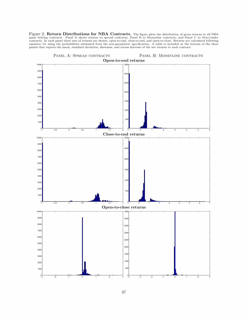
Figure 2: Return Distributions for NBA Contracts. The figure plots the distribution of gross returns to all NBAgame betting contracts. Panel A shows returns to spread contracts, Panel B to Moneyline contracts, and Panel C to Over/undercontracts. In each panel three sets of returns are shown: open-to-end, close-to-end, and open-to-close. Returns are calculated followingequation 13, using the probabilities estimated from the non-parametric specification. A table is included at the bottom of the threepanels that reports the mean, standard deviation, skewness, and excess kurtosis of the net returns to each contract.

Panel A: Spread contracts Panel B: Moneyline contractsOpen-to-end returns

−1 −0.5 0 0.5 1 1.5 20

1000

2000

3000

4000

5000

6000

7000

8000

9000

10000

−1 0 1 2 3 4 5 60

500

1000

1500

2000

2500

3000

3500

Close-to-end returns

−1 −0.5 0 0.5 1 1.5 20

1000

2000

3000

4000

5000

6000

7000

8000

9000

10000

−1 0 1 2 3 4 5 6 70

500

1000

1500

2000

2500

3000

Open-to-close returns

−3 −2 −1 0 1 2 30

1000

2000

3000

4000

5000

6000

7000

8000

9000

10000

−4 −3 −2 −1 0 1 2 30

500

1000

1500

2000

2500

3000

3500

4000

4500

37

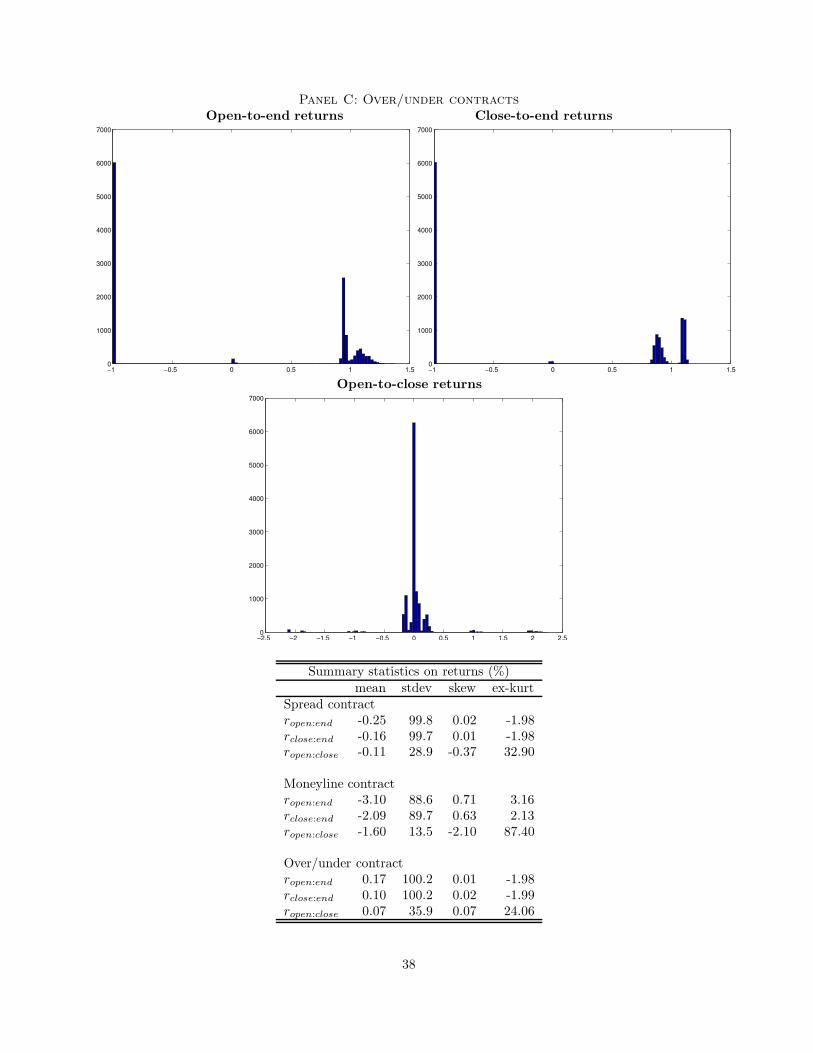
Panel C: Over/under contractsOpen-to-end returns Close-to-end returns

−1 −0.5 0 0.5 1 1.50

1000

2000

3000

4000

5000

6000

7000

−1 −0.5 0 0.5 1 1.50

1000

2000

3000

4000

5000

6000

7000

Open-to-close returns

−2.5 −2 −1.5 −1 −0.5 0 0.5 1 1.5 2 2.50

1000

2000

3000

4000

5000

6000

7000

Summary statistics on returns (%)

mean stdev skew ex-kurtSpread contractropen:end -0.25 99.8 0.02 -1.98rclose:end -0.16 99.7 0.01 -1.98ropen:close -0.11 28.9 -0.37 32.90

Moneyline contractropen:end -3.10 88.6 0.71 3.16rclose:end -2.09 89.7 0.63 2.13ropen:close -1.60 13.5 -2.10 87.40

Over/under contractropen:end 0.17 100.2 0.01 -1.98rclose:end 0.10 100.2 0.02 -1.99ropen:close 0.07 35.9 0.07 24.06

38

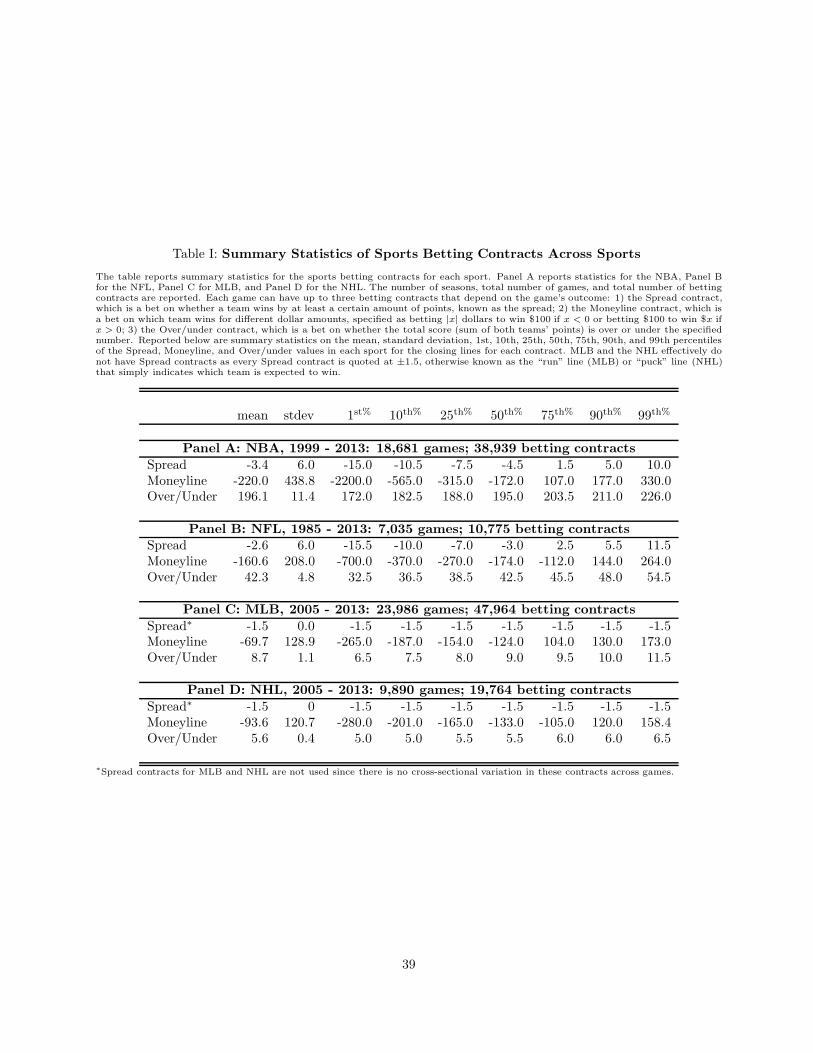
Table I: Summary Statistics of Sports Betting Contracts Across Sports

The table reports summary statistics for the sports betting contracts for each sport. Panel A reports statistics for the NBA, Panel Bfor the NFL, Panel C for MLB, and Panel D for the NHL. The number of seasons, total number of games, and total number of bettingcontracts are reported. Each game can have up to three betting contracts that depend on the game’s outcome: 1) the Spread contract,which is a bet on whether a team wins by at least a certain amount of points, known as the spread; 2) the Moneyline contract, which isa bet on which team wins for different dollar amounts, specified as betting |x| dollars to win $100 if x < 0 or betting $100 to win $x ifx > 0; 3) the Over/under contract, which is a bet on whether the total score (sum of both teams’ points) is over or under the specifiednumber. Reported below are summary statistics on the mean, standard deviation, 1st, 10th, 25th, 50th, 75th, 90th, and 99th percentilesof the Spread, Moneyline, and Over/under values in each sport for the closing lines for each contract. MLB and the NHL effectively donot have Spread contracts as every Spread contract is quoted at ±1.5, otherwise known as the “run” line (MLB) or “puck” line (NHL)that simply indicates which team is expected to win.

mean stdev 1st% 10th% 25th% 50th% 75th% 90th% 99th%

Panel A: NBA, 1999 - 2013: 18,681 games; 38,939 betting contracts

Spread -3.4 6.0 -15.0 -10.5 -7.5 -4.5 1.5 5.0 10.0Moneyline -220.0 438.8 -2200.0 -565.0 -315.0 -172.0 107.0 177.0 330.0Over/Under 196.1 11.4 172.0 182.5 188.0 195.0 203.5 211.0 226.0

Panel B: NFL, 1985 - 2013: 7,035 games; 10,775 betting contractsSpread -2.6 6.0 -15.5 -10.0 -7.0 -3.0 2.5 5.5 11.5Moneyline -160.6 208.0 -700.0 -370.0 -270.0 -174.0 -112.0 144.0 264.0Over/Under 42.3 4.8 32.5 36.5 38.5 42.5 45.5 48.0 54.5

Panel C: MLB, 2005 - 2013: 23,986 games; 47,964 betting contracts

Spread∗ -1.5 0.0 -1.5 -1.5 -1.5 -1.5 -1.5 -1.5 -1.5Moneyline -69.7 128.9 -265.0 -187.0 -154.0 -124.0 104.0 130.0 173.0Over/Under 8.7 1.1 6.5 7.5 8.0 9.0 9.5 10.0 11.5

Panel D: NHL, 2005 - 2013: 9,890 games; 19,764 betting contracts

Spread∗ -1.5 0 -1.5 -1.5 -1.5 -1.5 -1.5 -1.5 -1.5Moneyline -93.6 120.7 -280.0 -201.0 -165.0 -133.0 -105.0 120.0 158.4Over/Under 5.6 0.4 5.0 5.0 5.5 5.5 6.0 6.0 6.5

∗Spread contracts for MLB and NHL are not used since there is no cross-sectional variation in these contracts across games.

39

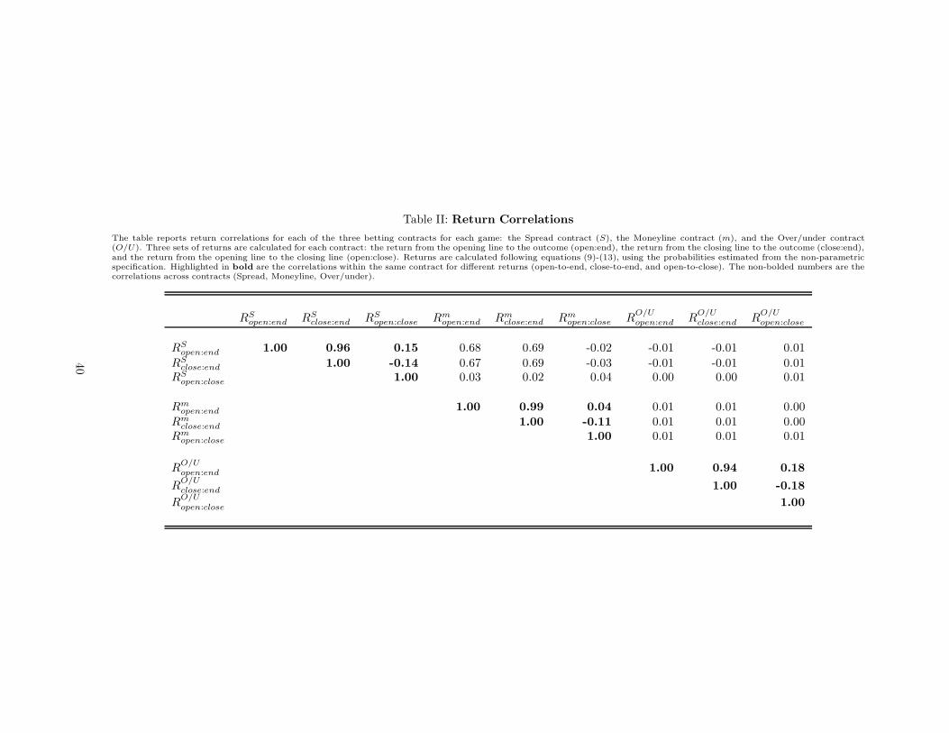
Table II: Return Correlations

The table reports return correlations for each of the three betting contracts for each game: the Spread contract (S), the Moneyline contract (m), and the Over/under contract(O/U). Three sets of returns are calculated for each contract: the return from the opening line to the outcome (open:end), the return from the closing line to the outcome (close:end),and the return from the opening line to the closing line (open:close). Returns are calculated following equations (9)-(13), using the probabilities estimated from the non-parametricspecification. Highlighted in bold are the correlations within the same contract for different returns (open-to-end, close-to-end, and open-to-close). The non-bolded numbers are thecorrelations across contracts (Spread, Moneyline, Over/under).

RSopen:end RS

close:end RSopen:close Rm

open:end Rmclose:end Rm

open:close RO/Uopen:end R

O/Uclose:end R

O/Uopen:close

RSopen:end 1.00 0.96 0.15 0.68 0.69 -0.02 -0.01 -0.01 0.01

RSclose:end 1.00 -0.14 0.67 0.69 -0.03 -0.01 -0.01 0.01

RSopen:close 1.00 0.03 0.02 0.04 0.00 0.00 0.01

Rmopen:end 1.00 0.99 0.04 0.01 0.01 0.00

Rmclose:end 1.00 -0.11 0.01 0.01 0.00

Rmopen:close 1.00 0.01 0.01 0.01

RO/Uopen:end 1.00 0.94 0.18

RO/Uclose:end 1.00 -0.18

RO/Uopen:close 1.00

40

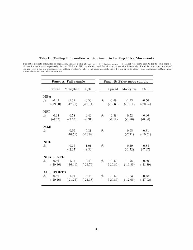
Table III: Testing Information vs. Sentiment in Betting Price Movements

The table reports estimates of regression equation (4): Rclose:end = α + β1Ropen:close + ε. Panel A reports results for the full sampleof bets for each sport separately, for the NBA and NFL combined, and for all four sports simultaneously. Panel B reports estimates ofthe regression for the subsample of betting contracts where the price actually moved from open to close—e.g., excluding betting lineswhere there was no price movement.

Panel A: Full sample Panel B: Price move sample

Spread Moneyline O/U Spread Moneyline O/U

NBAβ1 -0.49 -1.32 -0.50 β1 -0.49 -1.43 -0.50

(-19.30) (-17.91) (-20.14) (-19.68) (-18.11) (-20.24)

NFLβ1 -0.34 -0.58 -0.46 β1 -0.38 -0.52 -0.46

(-6.32) (-2.55) (-8.31) (-7.19) (-1.90) (-8.34)

MLBβ1 -0.95 -0.31 β1 -0.95 -0.31

(-10.51) (-10.09) (-7.11) (-10.51)

NHLβ1 -0.26 -1.01 β1 -0.19 -0.84

(-2.37) (-8.30) (-1.72) (-7.47)

NBA + NFLβ1 -0.46 -1.15 -0.49 β1 -0.47 -1.28 -0.50

(-20.16) (-16.41) (-21.79) (-20.86) (-16.89) (-21.89)

ALL SPORTSβ1 -0.46 -1.04 -0.44 β1 -0.47 -1.23 -0.48

(-20.16) (-21.25) (-24.38) (-20.86) (-17.66) (-27.02)

41

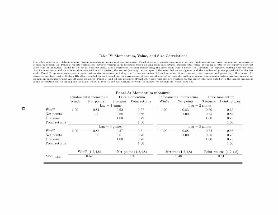
Table IV: Momentum, Value, and Size Correlations

The table reports correlations among various momentum, value, and size measures. Panel A reports correlations among various fundamental and price momentum measures asdefined in Section III. Panel B reports correlations between various value measures based on long-term past returns, fundamental ratios, including a ratio of the expected contractprice from an analytical model to the actual contract price, and a regression residual representing the error term from a model that predicts the expected betting contract pricethat includes home and away team dummies within each season, the record (winning percentage) of the team before each game, and the number of games played within the lastweek. Panel C reports correlations between various size measures, including the Forbes’ estimates of franchise value, ticket revenue, total revenue, and player payroll expense. Allmeasures are described in Section III. Also reported for each panel are the correlations of each variable or set of variables with a principal component-weighted average index of allmomentum measures (Panel A), all value measures (Panel B) and all size measures (Panel C), where variables are weighted by the eigenvector associated with the largest eigenvalueof the correlation matrix among the variables. Panel D reports the correlations between the indices for momentum, value, and size.

Panel A: Momentum measuresFundamental momentum Price momentum Fundamental momentum Price momentumWin% Net points $ returns Point returns Win% Net points $ returns Point returns

Lag = 1 game Lag = 2 gamesWin% 1.00 0.81 0.62 0.67 1.00 0.83 0.60 0.65Net points 1.00 0.68 0.86 1.00 0.65 0.82$ returns 1.00 0.79 1.00 0.78Point returns 1.00 1.00

Lag = 4 games Lag = 8 gamesWin% 1.00 0.85 0.57 0.61 1.00 0.88 0.52 0.56Net points 1.00 0.61 0.76 1.00 0.56 0.70$ returns 1.00 0.78 1.00 0.78Point returns 1.00 1.00

Win% (1,2,4,8) Net points (1,2,4,8) $returns (1,2,4,8) Point returns (1,2,4,8)Momindex 0.52 0.60 0.48 0.51

42

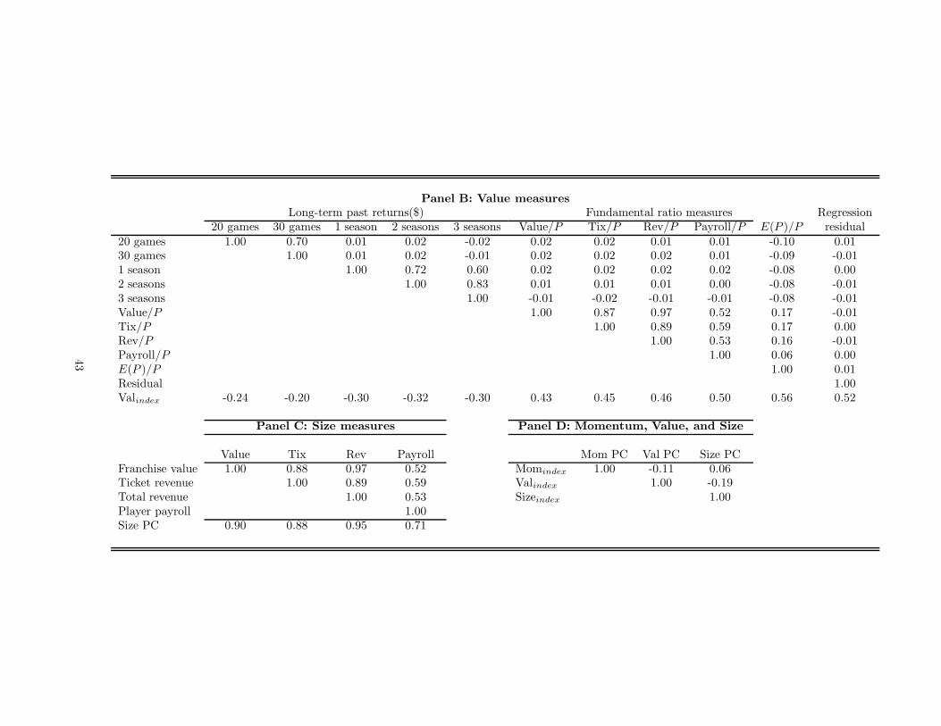
Panel B: Value measuresLong-term past returns($) Fundamental ratio measures Regression

20 games 30 games 1 season 2 seasons 3 seasons Value/P Tix/P Rev/P Payroll/P E(P )/P residual

20 games 1.00 0.70 0.01 0.02 -0.02 0.02 0.02 0.01 0.01 -0.10 0.0130 games 1.00 0.01 0.02 -0.01 0.02 0.02 0.02 0.01 -0.09 -0.011 season 1.00 0.72 0.60 0.02 0.02 0.02 0.02 -0.08 0.002 seasons 1.00 0.83 0.01 0.01 0.01 0.00 -0.08 -0.013 seasons 1.00 -0.01 -0.02 -0.01 -0.01 -0.08 -0.01Value/P 1.00 0.87 0.97 0.52 0.17 -0.01Tix/P 1.00 0.89 0.59 0.17 0.00Rev/P 1.00 0.53 0.16 -0.01Payroll/P 1.00 0.06 0.00E(P )/P 1.00 0.01Residual 1.00Valindex -0.24 -0.20 -0.30 -0.32 -0.30 0.43 0.45 0.46 0.50 0.56 0.52

Panel C: Size measures Panel D: Momentum, Value, and Size

Value Tix Rev Payroll Mom PC Val PC Size PCFranchise value 1.00 0.88 0.97 0.52 Momindex 1.00 -0.11 0.06Ticket revenue 1.00 0.89 0.59 Valindex 1.00 -0.19Total revenue 1.00 0.53 Sizeindex 1.00Player payroll 1.00Size PC 0.90 0.88 0.95 0.71

43

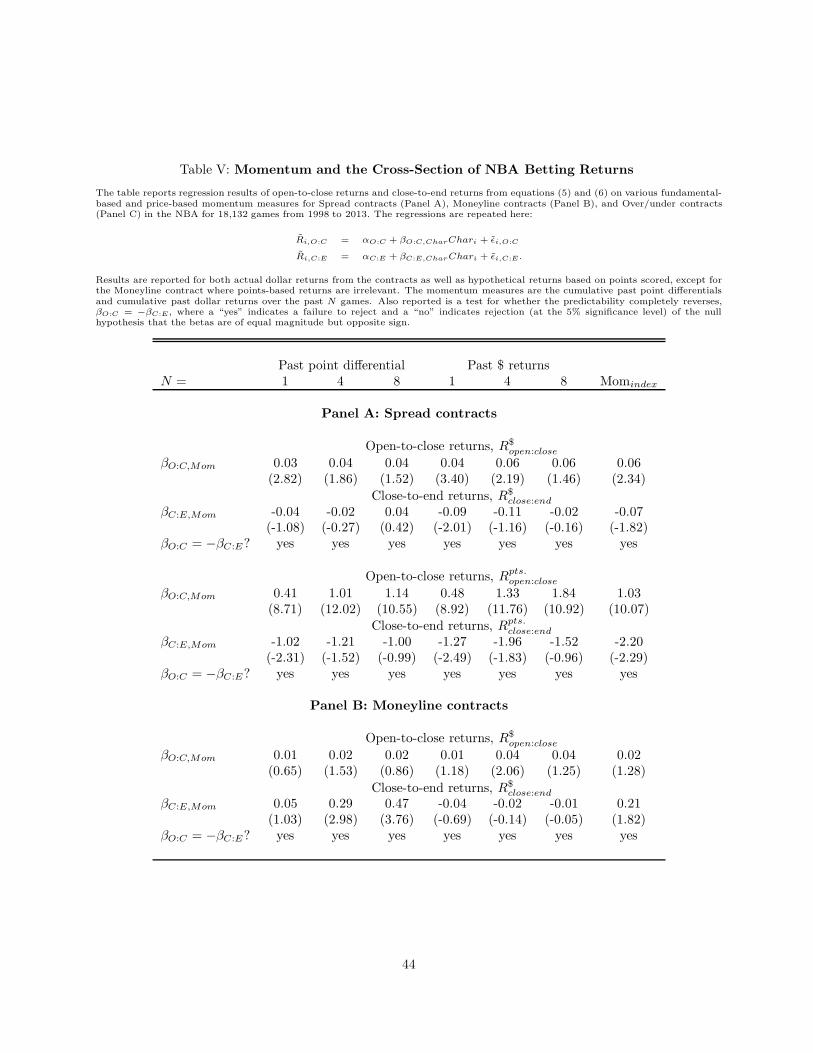
Table V: Momentum and the Cross-Section of NBA Betting Returns

The table reports regression results of open-to-close returns and close-to-end returns from equations (5) and (6) on various fundamental-based and price-based momentum measures for Spread contracts (Panel A), Moneyline contracts (Panel B), and Over/under contracts(Panel C) in the NBA for 18,132 games from 1998 to 2013. The regressions are repeated here:

R̃i,O:C = αO:C + βO:C,CharChari + ε̃i,O:C

R̃i,C:E = αC:E + βC:E,CharChari + ε̃i,C:E .

Results are reported for both actual dollar returns from the contracts as well as hypothetical returns based on points scored, except forthe Moneyline contract where points-based returns are irrelevant. The momentum measures are the cumulative past point differentialsand cumulative past dollar returns over the past N games. Also reported is a test for whether the predictability completely reverses,βO:C = −βC:E , where a “yes” indicates a failure to reject and a “no” indicates rejection (at the 5% significance level) of the nullhypothesis that the betas are of equal magnitude but opposite sign.

Past point differential Past $ returnsN = 1 4 8 1 4 8 Momindex

Panel A: Spread contracts

Open-to-close returns, R$open:close

βO:C,Mom 0.03 0.04 0.04 0.04 0.06 0.06 0.06(2.82) (1.86) (1.52) (3.40) (2.19) (1.46) (2.34)

Close-to-end returns, R$close:end

βC:E,Mom -0.04 -0.02 0.04 -0.09 -0.11 -0.02 -0.07(-1.08) (-0.27) (0.42) (-2.01) (-1.16) (-0.16) (-1.82)

βO:C = −βC:E? yes yes yes yes yes yes yes

Open-to-close returns, Rpts.open:close

βO:C,Mom 0.41 1.01 1.14 0.48 1.33 1.84 1.03(8.71) (12.02) (10.55) (8.92) (11.76) (10.92) (10.07)

Close-to-end returns, Rpts.close:end

βC:E,Mom -1.02 -1.21 -1.00 -1.27 -1.96 -1.52 -2.20(-2.31) (-1.52) (-0.99) (-2.49) (-1.83) (-0.96) (-2.29)

βO:C = −βC:E? yes yes yes yes yes yes yes

Panel B: Moneyline contracts

Open-to-close returns, R$open:close

βO:C,Mom 0.01 0.02 0.02 0.01 0.04 0.04 0.02(0.65) (1.53) (0.86) (1.18) (2.06) (1.25) (1.28)

Close-to-end returns, R$close:end

βC:E,Mom 0.05 0.29 0.47 -0.04 -0.02 -0.01 0.21(1.03) (2.98) (3.76) (-0.69) (-0.14) (-0.05) (1.82)

βO:C = −βC:E? yes yes yes yes yes yes yes

44

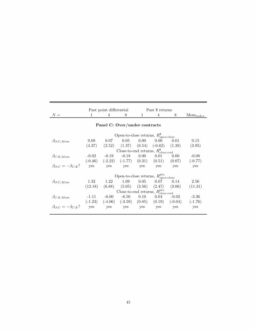
Past point differential Past $ returnsN = 1 4 8 1 4 8 Momindex

Panel C: Over/under contracts

Open-to-close returns, R$open:close

βO:C,Mom 0.08 0.07 0.05 0.00 0.00 0.01 0.15(4.37) (2.52) (1.37) (0.54) (-0.62) (1.28) (3.95)

Close-to-end returns, R$close:end

βC:E,Mom -0.02 -0.19 -0.18 0.00 0.01 0.00 -0.08(-0.46) (-2.22) (-1.77) (0.31) (0.51) (0.07) (-0.77)

βO:C = −βC:E? yes yes yes yes yes yes yes

Open-to-close returns, Rpts.open:close

βO:C,Mom 1.32 1.22 1.09 0.05 0.07 0.14 2.56(12.18) (6.88) (5.05) (3.56) (2.47) (3.06) (11.31)

Close-to-end returns, Rpts.close:end

βC:E,Mom -1.11 -6.00 -6.50 0.10 0.04 -0.02 -3.36(-1.23) (-4.06) (-3.59) (0.85) (0.19) (-0.04) (-1.76)

βO:C = −βC:E? yes yes yes yes yes yes yes

45

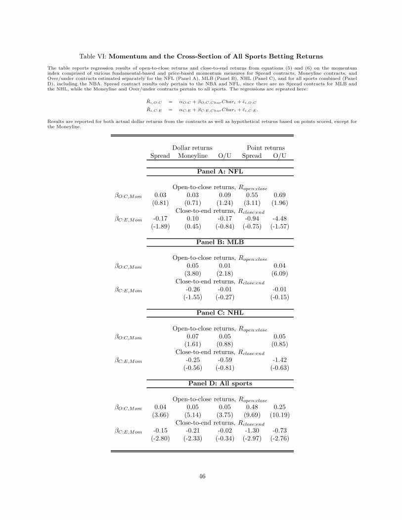
Table VI: Momentum and the Cross-Section of All Sports Betting Returns

The table reports regression results of open-to-close returns and close-to-end returns from equations (5) and (6) on the momentumindex comprised of various fundamental-based and price-based momentum measures for Spread contracts, Moneyline contracts, andOver/under contracts estimated separately for the NFL (Panel A), MLB (Panel B), NHL (Panel C), and for all sports combined (PanelD), including the NBA. Spread contract results only pertain to the NBA and NFL, since there are no Spread contracts for MLB andthe NHL, while the Moneyline and Over/under contracts pertain to all sports. The regressions are repeated here:

R̃i,O:C = αO:C + βO:C,CharChari + ε̃i,O:C

R̃i,C:E = αC:E + βC:E,CharChari + ε̃i,C:E .

Results are reported for both actual dollar returns from the contracts as well as hypothetical returns based on points scored, except forthe Moneyline.

Dollar returns Point returnsSpread Moneyline O/U Spread O/U

Panel A: NFL

Open-to-close returns, Ropen:close

βO:C,Mom 0.03 0.03 0.09 0.55 0.69(0.81) (0.71) (1.24) (3.11) (1.96)

Close-to-end returns, Rclose:end

βC:E,Mom -0.17 0.10 -0.17 -0.94 -4.48(-1.89) (0.45) (-0.84) (-0.75) (-1.57)

Panel B: MLB

Open-to-close returns, Ropen:close

βO:C,Mom 0.05 0.01 0.04(3.80) (2.18) (6.09)

Close-to-end returns, Rclose:end

βC:E,Mom -0.26 -0.01 -0.01(-1.55) (-0.27) (-0.15)

Panel C: NHL

Open-to-close returns, Ropen:close

βO:C,Mom 0.07 0.05 0.05(1.61) (0.88) (0.85)

Close-to-end returns, Rclose:end

βC:E,Mom -0.25 -0.59 -1.42(-0.56) (-0.81) (-0.63)

Panel D: All sports

Open-to-close returns, Ropen:close

βO:C,Mom 0.04 0.05 0.05 0.48 0.25(3.66) (5.14) (3.75) (9.69) (10.19)

Close-to-end returns, Rclose:end

βC:E,Mom -0.15 -0.21 -0.02 -1.30 -0.73(-2.80) (-2.33) (-0.34) (-2.97) (-2.76)

46

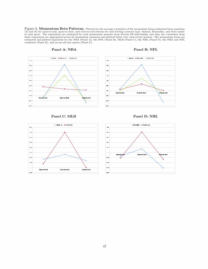
Figure 3: Momentum Beta Patterns. Plotted are the average t-statistics of the momentum betas estimated from equations(5) and (6) for open-to-end, open-to-close, and close-to-end returns for each betting contract type: Spread, Moneyline, and Over/underin each sport. The regressions are estimated for each momentum measure from Section III individually and then the t-statistics fromthese regressions are aggregated across all momentum measures and plotted below over each return horizon. The momentum betas areestimated and plotted separately for the NBA (Panel A), the NFL (Panel B), MLB (Panel C), the NHL (Panel D), the NBA and NFLcombined (Panel E), and across all four sports (Panel F).

Panel A: NBA Panel B: NFL

� � � � �

� � � � �

� � � �

� � � �

� � � �

� � � �

� � � �

� � � �

� � � �

� � �

� � � � � � � � � � � � � � � � � � � � � � � � � � � � � �

� � � � � � � � � � � ! � � " # � � $ % � � � �

& ' ( ) *

& ' ( * *

& * ( ) *

* ( * *

* ( ) *

' ( * *

' ( ) *

+ ( * *

+ ( ) *

, ( * *

- . / 0 1 2 3 1 / 0 4 - . / 0 1 2 3 1 5 6 3 7 / 8 6 3 7 / 1 2 3 1 / 0 4

9 : ; < = > ? @ A < B C D A < E F < ; G H A > < ;

Panel C: MLB Panel D: NHL

I J K L L M

N

J K L L

O K L L

P K L L

Q K L L

R K L L

S K L L

T K L L

U K L L

V W X Y Z [ \ Z X Y ] V W X Y Z [ \ Z ^ _ \ ` X a _ \ ` X Z [ \ Z X Y ]

b c d e f g h d e i j e k l m d n e k

o p q r p s

o p q t p s

o p q u p s

o p q v p s

w

p q v p

p q u p

p q t p

p q r p

x q p p

y z { | } ~ � } { | � y z { | } ~ � } � � � � { � � � � { } ~ � } { | �

� � � � � � � � � � � � � � � � � � �

47

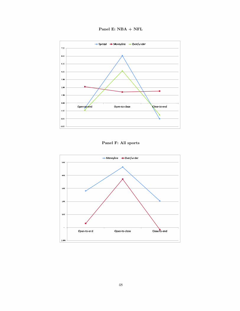
Panel E: NBA + NFL

� � � � �

� � � � �

� � � � �

� � � �

� � � �

� � � �

� � � �

� � � �

� � � �

� � � �

� � � �

� � � �   ¡ ¢   � � £ � � � �   ¡ ¢   ¤ ¥ ¢ ¦ � § ¥ ¢ ¦ �   ¡ ¢   � � £

¨ � © � ª £ « ¢ � � ¬ ¥ ­ � � � ® � © ¯ ° � £ � ©

Panel F: All sports

± ² ³ ´ ´ µ

¶

² ³ ´ ´

· ³ ´ ´

¸ ³ ´ ´

¹ ³ ´ ´

º ³ ´ ´

» ¼ ½ ¾ ¿ À Á ¿ ½ ¾ Â » ¼ ½ ¾ ¿ À Á ¿ Ã Ä Á Å ½ Æ Ä Á Å ½ ¿ À Á ¿ ½ ¾ Â

Ç Á ¾ ½ È Ä É ¾ ½ » Ê ½ Ë Ì Í ¾ Â ½ Ë

48

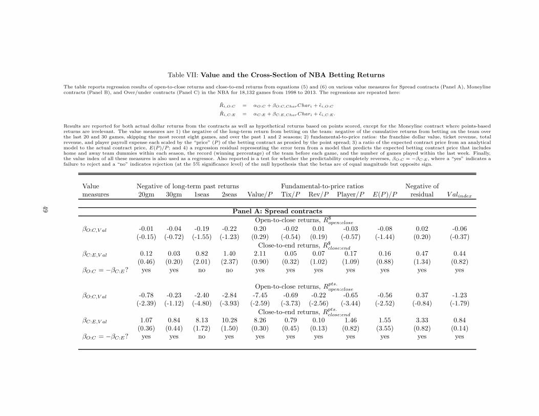
Table VII: Value and the Cross-Section of NBA Betting Returns

The table reports regression results of open-to-close returns and close-to-end returns from equations (5) and (6) on various value measures for Spread contracts (Panel A), Moneylinecontracts (Panel B), and Over/under contracts (Panel C) in the NBA for 18,132 games from 1998 to 2013. The regressions are repeated here:

R̃i,O:C = αO:C + βO:C,CharChari + ε̃i,O:C

R̃i,C:E = αC:E + βC:E,CharChari + ε̃i,C:E .

Results are reported for both actual dollar returns from the contracts as well as hypothetical returns based on points scored, except for the Moneyline contract where points-basedreturns are irrelevant. The value measures are 1) the negative of the long-term return from betting on the team: negative of the cumulative returns from betting on the team overthe last 20 and 30 games, skipping the most recent eight games, and over the past 1 and 2 seasons; 2) fundamental-to-price ratios: the franchise dollar value, ticket revenue, totalrevenue, and player payroll expense each scaled by the “price” (P) of the betting contract as proxied by the point spread; 3) a ratio of the expected contract price from an analyticalmodel to the actual contract price, E(P)/P ; and 4) a regression residual representing the error term from a model that predicts the expected betting contract price that includeshome and away team dummies within each season, the record (winning percentage) of the team before each game, and the number of games played within the last week. Finally,the value index of all these measures is also used as a regressor. Also reported is a test for whether the predictability completely reverses, βO:C = −βC:E , where a “yes” indicates afailure to reject and a “no” indicates rejection (at the 5% significance level) of the null hypothesis that the betas are of equal magnitude but opposite sign.

Value Negative of long-term past returns Fundamental-to-price ratios Negative ofmeasures 20gm 30gm 1seas 2seas Value/P Tix/P Rev/P Player/P E(P )/P residual V alindex

Panel A: Spread contracts

Open-to-close returns, R$open:close

βO:C,V al -0.01 -0.04 -0.19 -0.22 0.20 -0.02 0.01 -0.03 -0.08 0.02 -0.06(-0.15) (-0.72) (-1.55) (-1.23) (0.29) (-0.54) (0.19) (-0.57) (-1.44) (0.20) (-0.37)

Close-to-end returns, R$close:end

βC:E,V al 0.12 0.03 0.82 1.40 2.11 0.05 0.07 0.17 0.16 0.47 0.44(0.46) (0.20) (2.01) (2.37) (0.90) (0.32) (1.02) (1.09) (0.88) (1.34) (0.82)

βO:C = −βC:E? yes yes no no yes yes yes yes yes yes yes

Open-to-close returns, Rpts.open:close

βO:C,V al -0.78 -0.23 -2.40 -2.84 -7.45 -0.69 -0.22 -0.65 -0.56 0.37 -1.23(-2.39) (-1.12) (-4.80) (-3.93) (-2.59) (-3.73) (-2.56) (-3.44) (-2.52) (-0.84) (-1.79)

Close-to-end returns, Rpts.close:end

βC:E,V al 1.07 0.84 8.13 10.28 8.26 0.79 0.10 1.46 1.55 3.33 0.84(0.36) (0.44) (1.72) (1.50) (0.30) (0.45) (0.13) (0.82) (3.55) (0.82) (0.14)

βO:C = −βC:E? yes yes no yes yes yes yes yes yes yes yes

49

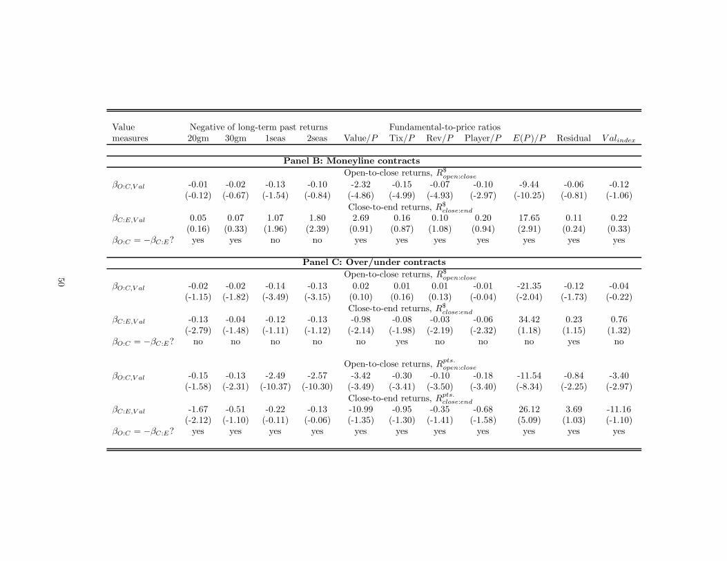
Value Negative of long-term past returns Fundamental-to-price ratiosmeasures 20gm 30gm 1seas 2seas Value/P Tix/P Rev/P Player/P E(P )/P Residual V alindex

Panel B: Moneyline contracts

Open-to-close returns, R$open:close

βO:C,V al -0.01 -0.02 -0.13 -0.10 -2.32 -0.15 -0.07 -0.10 -9.44 -0.06 -0.12(-0.12) (-0.67) (-1.54) (-0.84) (-4.86) (-4.99) (-4.93) (-2.97) (-10.25) (-0.81) (-1.06)

Close-to-end returns, R$close:end

βC:E,V al 0.05 0.07 1.07 1.80 2.69 0.16 0.10 0.20 17.65 0.11 0.22(0.16) (0.33) (1.96) (2.39) (0.91) (0.87) (1.08) (0.94) (2.91) (0.24) (0.33)

βO:C = −βC:E? yes yes no no yes yes yes yes yes yes yes

Panel C: Over/under contracts

Open-to-close returns, R$open:close

βO:C,V al -0.02 -0.02 -0.14 -0.13 0.02 0.01 0.01 -0.01 -21.35 -0.12 -0.04(-1.15) (-1.82) (-3.49) (-3.15) (0.10) (0.16) (0.13) (-0.04) (-2.04) (-1.73) (-0.22)

Close-to-end returns, R$close:end

βC:E,V al -0.13 -0.04 -0.12 -0.13 -0.98 -0.08 -0.03 -0.06 34.42 0.23 0.76(-2.79) (-1.48) (-1.11) (-1.12) (-2.14) (-1.98) (-2.19) (-2.32) (1.18) (1.15) (1.32)

βO:C = −βC:E? no no no no no yes no no no yes no

Open-to-close returns, Rpts.open:close

βO:C,V al -0.15 -0.13 -2.49 -2.57 -3.42 -0.30 -0.10 -0.18 -11.54 -0.84 -3.40(-1.58) (-2.31) (-10.37) (-10.30) (-3.49) (-3.41) (-3.50) (-3.40) (-8.34) (-2.25) (-2.97)

Close-to-end returns, Rpts.close:end

βC:E,V al -1.67 -0.51 -0.22 -0.13 -10.99 -0.95 -0.35 -0.68 26.12 3.69 -11.16(-2.12) (-1.10) (-0.11) (-0.06) (-1.35) (-1.30) (-1.41) (-1.58) (5.09) (1.03) (-1.10)

βO:C = −βC:E? yes yes yes yes yes yes yes yes yes yes yes

50

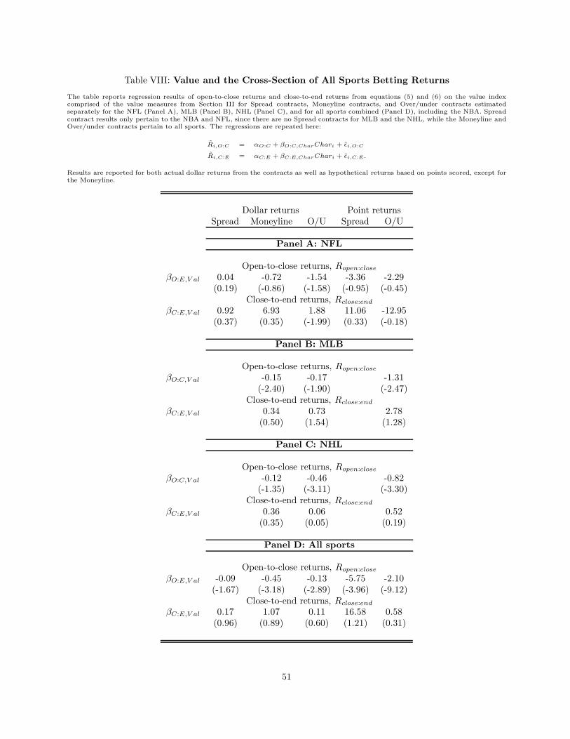
Table VIII: Value and the Cross-Section of All Sports Betting Returns

The table reports regression results of open-to-close returns and close-to-end returns from equations (5) and (6) on the value indexcomprised of the value measures from Section III for Spread contracts, Moneyline contracts, and Over/under contracts estimatedseparately for the NFL (Panel A), MLB (Panel B), NHL (Panel C), and for all sports combined (Panel D), including the NBA. Spreadcontract results only pertain to the NBA and NFL, since there are no Spread contracts for MLB and the NHL, while the Moneyline andOver/under contracts pertain to all sports. The regressions are repeated here:

R̃i,O:C = αO:C + βO:C,CharChari + ε̃i,O:C

R̃i,C:E = αC:E + βC:E,CharChari + ε̃i,C:E .

Results are reported for both actual dollar returns from the contracts as well as hypothetical returns based on points scored, except forthe Moneyline.

Dollar returns Point returnsSpread Moneyline O/U Spread O/U

Panel A: NFL

Open-to-close returns, Ropen:close

βO:E,V al 0.04 -0.72 -1.54 -3.36 -2.29(0.19) (-0.86) (-1.58) (-0.95) (-0.45)

Close-to-end returns, Rclose:end

βC:E,V al 0.92 6.93 1.88 11.06 -12.95(0.37) (0.35) (-1.99) (0.33) (-0.18)

Panel B: MLB

Open-to-close returns, Ropen:close

βO:C,V al -0.15 -0.17 -1.31(-2.40) (-1.90) (-2.47)

Close-to-end returns, Rclose:end

βC:E,V al 0.34 0.73 2.78(0.50) (1.54) (1.28)

Panel C: NHL

Open-to-close returns, Ropen:close

βO:C,V al -0.12 -0.46 -0.82(-1.35) (-3.11) (-3.30)

Close-to-end returns, Rclose:end

βC:E,V al 0.36 0.06 0.52(0.35) (0.05) (0.19)

Panel D: All sports

Open-to-close returns, Ropen:close

βO:E,V al -0.09 -0.45 -0.13 -5.75 -2.10(-1.67) (-3.18) (-2.89) (-3.96) (-9.12)

Close-to-end returns, Rclose:end

βC:E,V al 0.17 1.07 0.11 16.58 0.58(0.96) (0.89) (0.60) (1.21) (0.31)

51

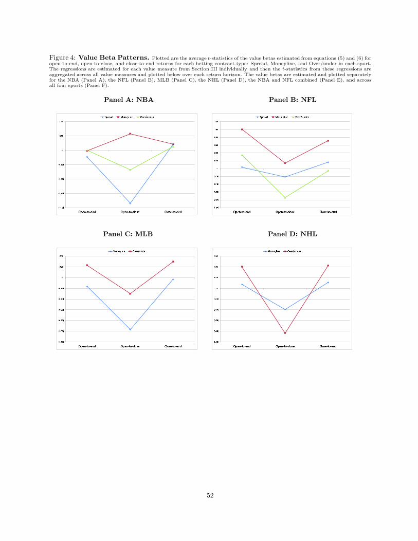
Figure 4: Value Beta Patterns. Plotted are the average t-statistics of the value betas estimated from equations (5) and (6) foropen-to-end, open-to-close, and close-to-end returns for each betting contract type: Spread, Moneyline, and Over/under in each sport.The regressions are estimated for each value measure from Section III individually and then the t-statistics from these regressions areaggregated across all value measures and plotted below over each return horizon. The value betas are estimated and plotted separatelyfor the NBA (Panel A), the NFL (Panel B), MLB (Panel C), the NHL (Panel D), the NBA and NFL combined (Panel E), and acrossall four sports (Panel F).

Panel A: NBA Panel B: NFL

Î Ï Ð Ñ Ñ Ò

Î Ó Ð Ô Ñ Ò

Î Ó Ð Ñ Ñ Ò

Î Ñ Ð Ô Ñ Ò

Õ

Ñ Ð Ô Ñ

Ó Ð Ñ Ñ

Ö × Ø Ù Ú Û Ü Ú Ø Ù Ý Ö × Ø Ù Ú Û Ü Ú Þ ß Ü à Ø á ß Ü à Ø Ú Û Ü Ú Ø Ù Ý

â ã ä å æ ç è é ê å ë ì í ê å î ï å ä ð ñ ê ç å ä

ò ó ô õ õ öò õ ô ÷ õ öò õ ô ø õ öò õ ô ù õ öò õ ô ú õ ö

û

õ ô ú õõ ô ù õõ ô ø õõ ô ÷ õó ô õ õó ô ú õ

ü ý þ ÿ � � � � þ ÿ � ü ý þ ÿ � � � � � � � � þ � � � � þ � � � � þ ÿ �

� � � � � � � � � � � � � � � � � � �

Panel C: MLB Panel D: NHL

� � � � � �� � � � � �� � � � � �� � � � � �� � � � �� � � � � �

!� � � �� � �

" # $ % & ' ( & $ % ) " # $ % & ' ( & * + ( , $ - + ( , $ & ' ( & $ % )

. / 0 1 2 3 4 0 1 5 6 1 7 8 9 0 : 1 7

; < = > > ?; > = @ > ?; > = A > ?; > = B > ?; > = C > ?

D> = C >> = B >> = A >

E F G H I J K I G H L E F G H I J K I M N K O G P N K O G I J K I G H L

Q R S T U V W S T X Y T Z [ \ S ] T Z

52

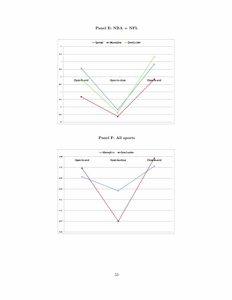
Panel E: NBA + NFL

^ _^ ` a b

^ `^ c a b

^ c^ d a b

dd a b

cc a b

`

e f g h i j k i g h l e f g h i j k i m n k o g p n k o g i j k i g h l

q f r g s l t k h g u n v h g e w g r x y h l g r

Panel F: All sports

z { | } }

z ~ | } }

z � | } }

z � | } }

z � | } }

z � | } }

z � | } }

} | } } � � � �� � � �

� � � � � � �� � � � � � � �

� �� � �

�� � � �

� � �� �

� �� � �

� � ��

� � ��

� � � �

53

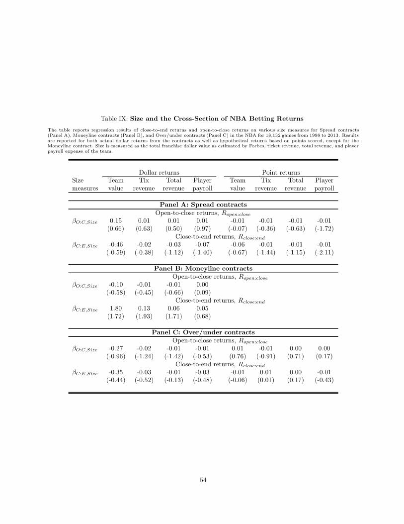
Table IX: Size and the Cross-Section of NBA Betting Returns

The table reports regression results of close-to-end returns and open-to-close returns on various size measures for Spread contracts(Panel A), Moneyline contracts (Panel B), and Over/under contracts (Panel C) in the NBA for 18,132 games from 1998 to 2013. Resultsare reported for both actual dollar returns from the contracts as well as hypothetical returns based on points scored, except for theMoneyline contract. Size is measured as the total franchise dollar value as estimated by Forbes, ticket revenue, total revenue, and playerpayroll expense of the team.

Dollar returns Point returnsSize Team Tix Total Player Team Tix Total Playermeasures value revenue revenue payroll value revenue revenue payroll

Panel A: Spread contracts

Open-to-close returns, Ropen:close

βO:C,Size 0.15 0.01 0.01 0.01 -0.01 -0.01 -0.01 -0.01(0.66) (0.63) (0.50) (0.97) (-0.07) (-0.36) (-0.63) (-1.72)

Close-to-end returns, Rclose:end

βC:E,Size -0.46 -0.02 -0.03 -0.07 -0.06 -0.01 -0.01 -0.01(-0.59) (-0.38) (-1.12) (-1.40) (-0.67) (-1.44) (-1.15) (-2.11)

Panel B: Moneyline contractsOpen-to-close returns, Ropen:close

βO:C,Size -0.10 -0.01 -0.01 0.00(-0.58) (-0.45) (-0.66) (0.09)

Close-to-end returns, Rclose:end

βC:E,Size 1.80 0.13 0.06 0.05(1.72) (1.93) (1.71) (0.68)

Panel C: Over/under contractsOpen-to-close returns, Ropen:close

βO:C,Size -0.27 -0.02 -0.01 -0.01 0.01 -0.01 0.00 0.00(-0.96) (-1.24) (-1.42) (-0.53) (0.76) (-0.91) (0.71) (0.17)

Close-to-end returns, Rclose:end

βC:E,Size -0.35 -0.03 -0.01 -0.03 -0.01 0.01 0.00 -0.01(-0.44) (-0.52) (-0.13) (-0.48) (-0.06) (0.01) (0.17) (-0.43)

54

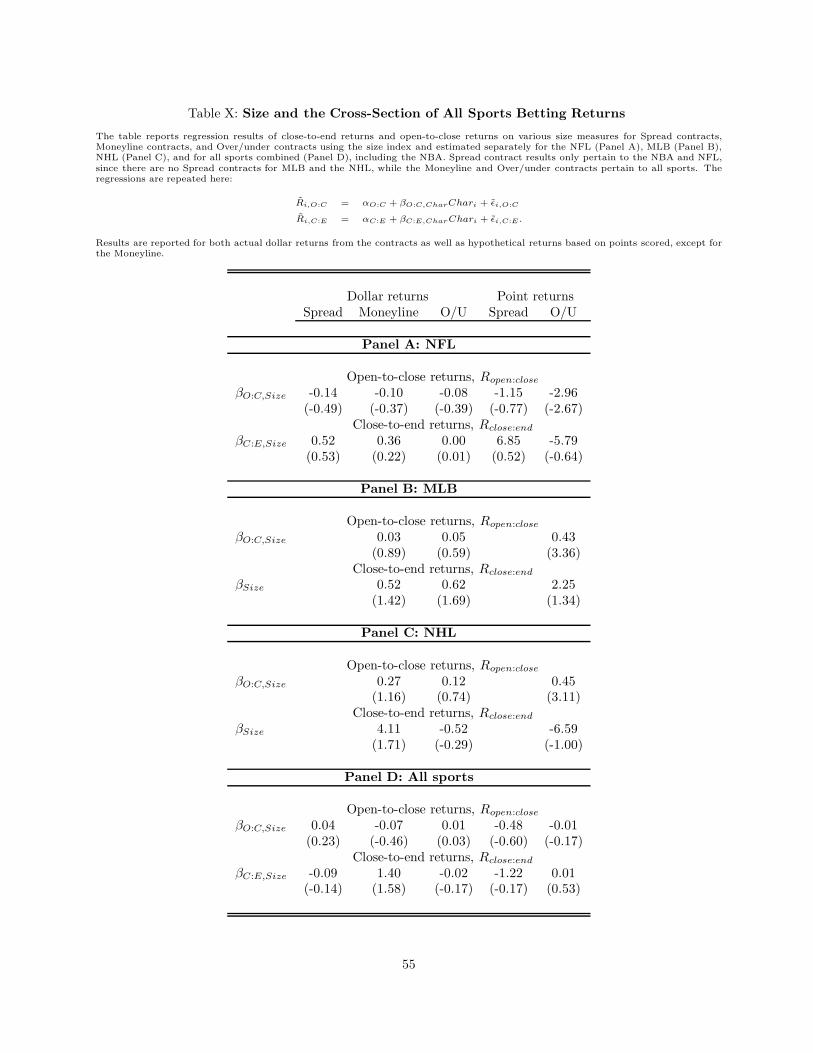
Table X: Size and the Cross-Section of All Sports Betting Returns

The table reports regression results of close-to-end returns and open-to-close returns on various size measures for Spread contracts,Moneyline contracts, and Over/under contracts using the size index and estimated separately for the NFL (Panel A), MLB (Panel B),NHL (Panel C), and for all sports combined (Panel D), including the NBA. Spread contract results only pertain to the NBA and NFL,since there are no Spread contracts for MLB and the NHL, while the Moneyline and Over/under contracts pertain to all sports. Theregressions are repeated here:

R̃i,O:C = αO:C + βO:C,CharChari + ε̃i,O:C

R̃i,C:E = αC:E + βC:E,CharChari + ε̃i,C:E .

Results are reported for both actual dollar returns from the contracts as well as hypothetical returns based on points scored, except forthe Moneyline.

Dollar returns Point returnsSpread Moneyline O/U Spread O/U

Panel A: NFL

Open-to-close returns, Ropen:close

βO:C,Size -0.14 -0.10 -0.08 -1.15 -2.96(-0.49) (-0.37) (-0.39) (-0.77) (-2.67)

Close-to-end returns, Rclose:end

βC:E,Size 0.52 0.36 0.00 6.85 -5.79(0.53) (0.22) (0.01) (0.52) (-0.64)

Panel B: MLB

Open-to-close returns, Ropen:close

βO:C,Size 0.03 0.05 0.43(0.89) (0.59) (3.36)

Close-to-end returns, Rclose:end

βSize 0.52 0.62 2.25(1.42) (1.69) (1.34)

Panel C: NHL

Open-to-close returns, Ropen:close

βO:C,Size 0.27 0.12 0.45(1.16) (0.74) (3.11)

Close-to-end returns, Rclose:end

βSize 4.11 -0.52 -6.59(1.71) (-0.29) (-1.00)

Panel D: All sports

Open-to-close returns, Ropen:close

βO:C,Size 0.04 -0.07 0.01 -0.48 -0.01(0.23) (-0.46) (0.03) (-0.60) (-0.17)

Close-to-end returns, Rclose:end

βC:E,Size -0.09 1.40 -0.02 -1.22 0.01(-0.14) (1.58) (-0.17) (-0.17) (0.53)

55

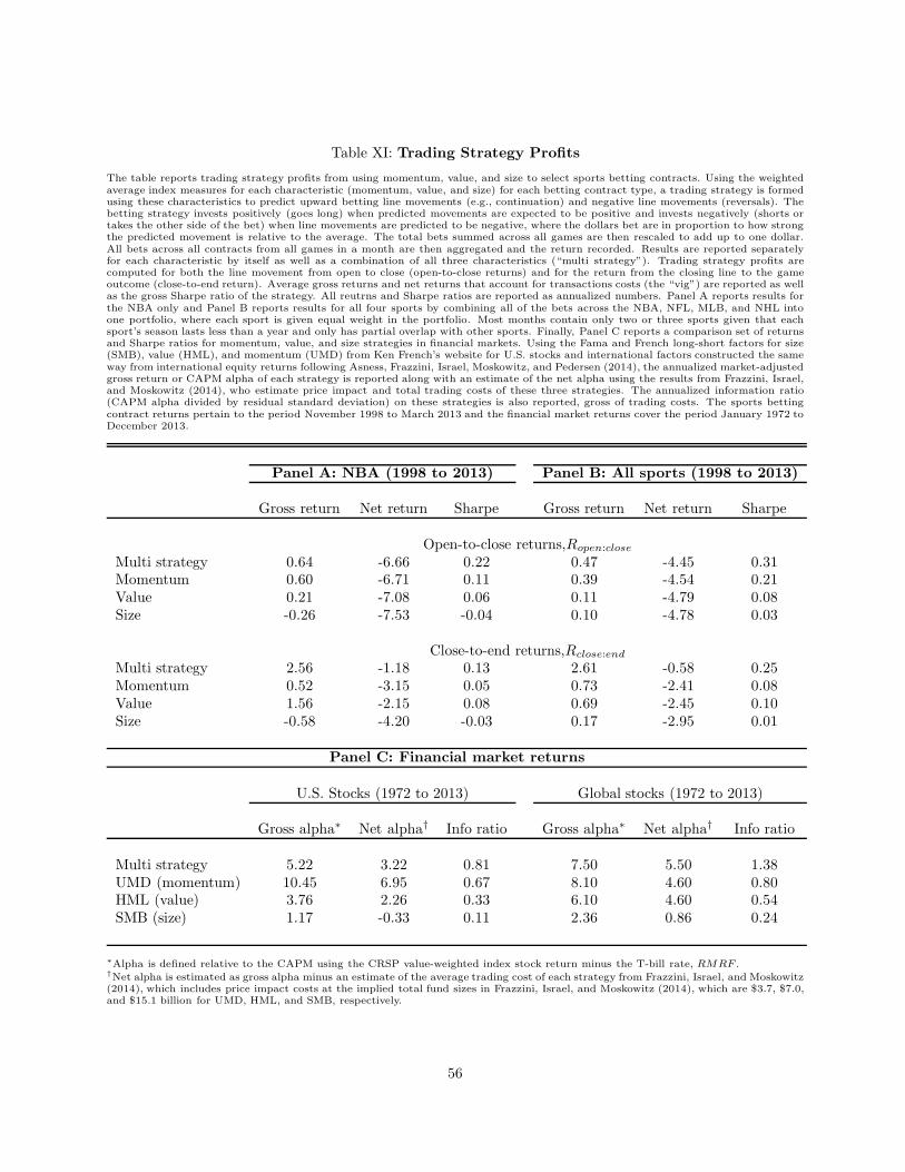
Table XI: Trading Strategy Profits

The table reports trading strategy profits from using momentum, value, and size to select sports betting contracts. Using the weightedaverage index measures for each characteristic (momentum, value, and size) for each betting contract type, a trading strategy is formedusing these characteristics to predict upward betting line movements (e.g., continuation) and negative line movements (reversals). Thebetting strategy invests positively (goes long) when predicted movements are expected to be positive and invests negatively (shorts ortakes the other side of the bet) when line movements are predicted to be negative, where the dollars bet are in proportion to how strongthe predicted movement is relative to the average. The total bets summed across all games are then rescaled to add up to one dollar.All bets across all contracts from all games in a month are then aggregated and the return recorded. Results are reported separatelyfor each characteristic by itself as well as a combination of all three characteristics (“multi strategy”). Trading strategy profits arecomputed for both the line movement from open to close (open-to-close returns) and for the return from the closing line to the gameoutcome (close-to-end return). Average gross returns and net returns that account for transactions costs (the “vig”) are reported as wellas the gross Sharpe ratio of the strategy. All reutrns and Sharpe ratios are reported as annualized numbers. Panel A reports results forthe NBA only and Panel B reports results for all four sports by combining all of the bets across the NBA, NFL, MLB, and NHL intoone portfolio, where each sport is given equal weight in the portfolio. Most months contain only two or three sports given that eachsport’s season lasts less than a year and only has partial overlap with other sports. Finally, Panel C reports a comparison set of returnsand Sharpe ratios for momentum, value, and size strategies in financial markets. Using the Fama and French long-short factors for size(SMB), value (HML), and momentum (UMD) from Ken French’s website for U.S. stocks and international factors constructed the sameway from international equity returns following Asness, Frazzini, Israel, Moskowitz, and Pedersen (2014), the annualized market-adjustedgross return or CAPM alpha of each strategy is reported along with an estimate of the net alpha using the results from Frazzini, Israel,and Moskowitz (2014), who estimate price impact and total trading costs of these three strategies. The annualized information ratio(CAPM alpha divided by residual standard deviation) on these strategies is also reported, gross of trading costs. The sports bettingcontract returns pertain to the period November 1998 to March 2013 and the financial market returns cover the period January 1972 toDecember 2013.

Panel A: NBA (1998 to 2013) Panel B: All sports (1998 to 2013)

Gross return Net return Sharpe Gross return Net return Sharpe

Open-to-close returns,Ropen:close

Multi strategy 0.64 -6.66 0.22 0.47 -4.45 0.31Momentum 0.60 -6.71 0.11 0.39 -4.54 0.21Value 0.21 -7.08 0.06 0.11 -4.79 0.08Size -0.26 -7.53 -0.04 0.10 -4.78 0.03

Close-to-end returns,Rclose:end

Multi strategy 2.56 -1.18 0.13 2.61 -0.58 0.25Momentum 0.52 -3.15 0.05 0.73 -2.41 0.08Value 1.56 -2.15 0.08 0.69 -2.45 0.10Size -0.58 -4.20 -0.03 0.17 -2.95 0.01

Panel C: Financial market returns

U.S. Stocks (1972 to 2013) Global stocks (1972 to 2013)

Gross alpha∗ Net alpha† Info ratio Gross alpha∗ Net alpha† Info ratio

Multi strategy 5.22 3.22 0.81 7.50 5.50 1.38UMD (momentum) 10.45 6.95 0.67 8.10 4.60 0.80HML (value) 3.76 2.26 0.33 6.10 4.60 0.54SMB (size) 1.17 -0.33 0.11 2.36 0.86 0.24

∗Alpha is defined relative to the CAPM using the CRSP value-weighted index stock return minus the T-bill rate, RMRF .†Net alpha is estimated as gross alpha minus an estimate of the average trading cost of each strategy from Frazzini, Israel, and Moskowitz(2014), which includes price impact costs at the implied total fund sizes in Frazzini, Israel, and Moskowitz (2014), which are $3.7, $7.0,and $15.1 billion for UMD, HML, and SMB, respectively.

56

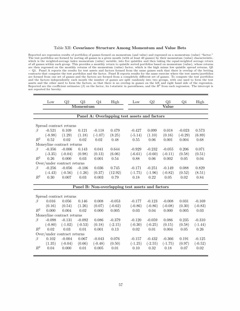
Table XII: Covariance Structure Among Momentum and Value Bets

Reported are regression results of portfolios of games formed on momentum (and value) and regressed on a momentum (value) “factor.”The test portfolios are formed by sorting all games in a given month (with at least 40 games) by their momentum (value) characteristic,which is the weighted-average index momentum (value) variable, into five quintiles and then taking the equal-weighted average returnof all games within each group. This provides a monthly return to quintile sorted portfolios based on momentum (value), whose returnsare then regressed on the monthly returns of the momentum (value) factor, which is the high minus low quintile spread returns, Q5− Q1. Panel A reports the results for test assets and factors formed from the same games such that there is overlap of the bettingcontracts that comprise the test portfolios and the factor. Panel B reports results for the same exercise where the test assets/portfoliosare formed from one set of games and the factors are formed from a completely different set of games. To compute the test portfoliosand the factors independently each month the number of games are split randomly into two groups, with one used to form the testassets and the other used to form the factors, so that there is no overlap in games on the left and right hand side of the regression.Reported are the coefficient estimates (β) on the factor, its t-statistic in parentheses, and the R2 from each regression. The intercept isnot reported for brevity.

Low Q2 Q3 Q4 High Low Q2 Q3 Q4 HighMomentum Value

Panel A: Overlapping test assets and factors

Spread contract returnsβ -0.521 0.109 0.121 -0.118 0.479 -0.427 0.099 0.018 -0.023 0.573

(-8.98) (1.29) (1.18) (-1.07) (8.25) (-5.14) (1.10) (0.16) (-0.29) (6.89)R2 0.52 0.02 0.02 0.02 0.48 0.55 0.06 0.001 0.004 0.68Moneyline contract returnsβ -0.356 -0.006 0.143 0.041 0.644 -0.929 -0.232 -0.055 0.206 0.071

(-3.35) (-0.04) (0.98) (0.13) (6.06) (-6.61) (-0.60) (-0.11) (0.58) (0.51)R2 0.26 0.000 0.03 0.001 0.54 0.88 0.06 0.002 0.05 0.04Over/under contract returnsβ -0.256 -0.056 -0.106 0.036 0.745 -0.171 -0.251 -0.149 0.088 0.829

(-4.43) (-0.56) (-1.26) (0.37) (12.92) (-1.75) (-1.96) (-0.82) (0.52) (8.51)R2 0.30 0.007 0.03 0.003 0.79 0.18 0.22 0.05 0.02 0.84

Panel B: Non-overlapping test assets and factors

Spread contract returnsβ 0.016 0.056 0.146 0.008 -0.053 -0.177 -0.123 -0.008 0.031 -0.169

(0.16) (0.54) (1.26) (0.07) (-0.62) (-0.86) (-0.86) (-0.08) (0.30) (-0.83)R2 0.000 0.004 0.02 0.000 0.005 0.03 0.04 0.000 0.005 0.03Moneyline contract returnsβ -0.098 -0.131 -0.092 0.086 -0.379 -0.120 -0.059 0.086 0.235 -0.310

(-0.80) (-1.02) (-0.53) (0.18) (-2.15) (-0.30) (-0.25) (0.15) (0.58) (-1.44)R2 0.02 0.03 0.01 0.001 0.13 0.02 0.01 0.004 0.05 0.26Over/under contract returnsβ 0.102 -0.004 0.067 -0.043 0.076 -0.157 -0.432 -0.366 0.191 -0.125

(1.35) (-0.04) (0.66) (-0.48) (0.50) (-1.25) (-2.55) (-1.75) (0.97) (-0.52)R2 0.04 0.000 0.01 0.005 0.01 0.10 0.32 0.18 0.07 0.02

57

Appendices

A Computing Prices and Returns

In order to compute returns, I first convert each contract line into a price by estimating the probability, π(St),

of a payoff occurring and calculating the expected value of the contract based on the probability and value

of each payoff state for that contract, where the payoff probability may depend on St, the time t betting line

(Spread, Moneyline, or Over/under value). For example, using equation (1) the price of a Spread contract at

the terminal date T is,

PST = (210) I {cover} + (110) I {push} + (0) I {fail} (9)

where I {cover} and I {push} are indicator functions for the payoff outcomes of the contract at time T . For

dates t < T before the terminal payoff the price of the Spread contract is,

PSt = 210× πcover (St) + 110× πpush (St) + 0 × πfail(St) (10)

where the probability of cover, push, and fail may vary with the value of the spread, St.

For Moneyline contracts, using equation (2) (assuming contracts payoff $100 if m < 0 and cost $100 for

m > 0) prices are

PmT = (|mT | + 100) I {win} + [max(mT , 100)] I {tie}

Pmt =

{(100 − mt)πwin (mt) + (−mt) πtie (mt) + 5 if mt < 0(100 + mt)πwin (mt) + (100)πtie (mt) + 5 if mt > 0

(11)

where mt is the moneyline value at time t and the +5 accounts for the vig charged to both sides of the

contract (assumed to be split evenly between both sides). A “tie” for the Moneyline contract means the two

teams actually tied, which is very rare for the sports I examine, hence I effectively ignore ties.22

Finally, the prices of Over/under contracts are very similar to those of Spread contracts. Using equation

(3) prices for betting on the “over” are,

PO/UT = (210) I {over} + (110) I {push} + (0) I {under}

PO/Ut = 210× πover (O/Ut) + 110× πpush (O/Ut) + 0 × πunder(O/Ut). (12)

Returns for all contracts c ∈ {S, m, O/U} over the three horizons above are then simply,

Rcopen:end =

P cT

P c0

, Rcclose:end =

P cT

P c1

, Rcopen:close =

P c1

P c0

. (13)

A. Estimating payoff probabilities

In order to calculate prices and returns from the above equations, I compute the probabilities of payoff states

for each contract for both opening and closing lines. Specifically, I compute cover and push probabilities for

opening and closing Spreads, home team win probabilities for opening and closing Moneylines, and over and

push probabilities for opening and closing Over/under totals.

I adopt two approaches for computing probabilities. The first is a theoretical approach, where I assume

that contract prices are set such that the odds of winning and losing each bet are equal. The second approach

22Across all of the 59,592 games in the dataset, only 10 games ended in a tie, and only five of those had opening betting lines,all of which are in the NFL. Ties are not allowed in the NBA, MLB, and are not allowed in the NHL since the 2005-2006 season,which is the start of the data, when the NHL instituted shoot outs at the end of tie games to eliminate ties. None of the resultsare affected by excluding the five tied games in the NFL.

58

is to empirically estimate the probabilities of the payoff states from the data. Levitt (2004) argues and finds

that bookmakers try to set their lines/prices such that each side has roughly an equal chance of winning, but

also shows that bookmakers will sometimes deviate from this strategy when they can better predict game

outcomes or betting interest. Hence, the theoretical equal probability approach likely captures the majority of

cases, while the empirical approach should capture any deviations from this, subject to estimation uncertainty.

In both cases, the probability assumptions will only affect the results if either model error or estimation error

is correlated with the cross-sectional characteristics I examine. As I will show, the returns (and all of the

results in the paper) are robust across a variety of probability estimation methods.

Appendix A details the probability estimates used in the paper. The first set come from theory and

assume an equal probability of winning and losing the bet for all betting lines. The second set are estimated

from the data under various models that include a logit, probit, and non-parametric kernel density estimator

(see Appendix A for details).

The four methods for computing probabilities obtain nearly identical results. For simplicity and brevity,

I report estimates only for the NBA contracts to illustrate the calculations, but Appendix A contains the

relevant estimates for the other sports, which show the same patterns. Panel A of Figure A1 plots the

probability of covering or pushing for Spread contracts at every spread value. A small amount of random

noise is added to each data point to gauge the number of contracts at each spread value. The probabilities

associated with full-point spreads and half-point spreads are indicated separately on the graphs, where because

half-point spreads cannot result in pushes, the estimated probabilities exhibit a jagged saw-tooth pattern as

spreads move from full-point to half-point values. Panels B and C of Figure A1 plot the probability of

winning the bet for opening and closing Moneylines and O/U contracts, respectively. (Pushing is not an

issue for Moneyline contracts [see the discussion in footnote 22], so I do not estimate push probabilities.) The

probability estimates are all very similar and match closely the theoretical ones. Given the probabilities of

the payoff states for each contract and betting line, I compute prices and returns using equations (9)–(13).

B. Probability Estimators

Theoretical probabilities. The first set of probabilities assumes all contract prices are set such that

winning and losing is roughly equal. Under this scenario, all contracts face the same probability of covering

or failing, so a spread of 20 points is just as likely to pay off as is a spread of two points. This turns out to

be very close to what bookmakers actually do, but there are some deviations (see Levitt (2004)), which I will

show below and take into account.

For spread and over/under payoff probabilities, I use 0.5 for cover and fail (or over and under) probabilities

for half-point spreads, where pushes are impossible. For full-point spreads, where a push is possible, I

first compute the empirical unconditional push probability for that contract type (separately for opening

and closing lines) using the full sample of data for all contracts facing the exact same point spread or

over/under total, where a minimum of five observations is required to compute this probability. Then, using

that empirical push probability I divide the remaining probability equally for winning and losing the bet,

π(cover) = π(fail) = (1 − π̂ (push)) /2.

For Moneyline contracts, where the probability of winning and losing is clearly not equal, since payoffs

adjust rather than spreads, I solve for π as follows:

(100)π (win) + (m) [1 − π (win)] = −5 if m < 0

(m)π (win) + (−100) [1 − π (win)] = −5 if m > 0

where m is the actual Moneyline quote. This simplifies to

π (win) =− (m + 5)

100− mif m < 0

59

π (win) =95

100 + mif m > 0.

The assumption here is that payoffs × probability are set to equal half of the commission or vig on both sides

of the contract.

Empirically estimated probabilities. Rather than assume all probabilities of winning or losing the

bet are the same across all lines, I also estimate empirically the probability of payoffs for different lines, to

take into account that bookmakers may deviate from equal probability bets.

For Spread contracts, for example, I estimate from the data the frequency of cover, push, and fail for all

contracts facing the same spread for all spreads within each sport. The assumption here is that probabilities

for a given spread are the same across games within a given sport. This is similar in spirit to the literature

that tries to recover real probabilities from risk-neutral probabilities from option contracts (e.g., Ross (2013),

Andersen, Fusari, and Todorov (2014), Borovicka, Hansen, and Scheinkman (2014)). However, the difference

here is that sports betting contracts are not confounded by risk premia, hence extraction of the true prob-

abilities from prices is simpler. However, since some spreads have a limited number of observations, it is

difficult to reliably use sample frequencies to estimate probabilities at all spreads.23 Therefore, I use several

discrete choice models—logit, probit, and a non-parametric Gaussian kernel density estimator—to estimate

probabilities. Specifically, I require a minimum of five observations for each spread, and estimate probabilities

of payoff states for each opening and closing line for each contract under each of the three discrete choice

models. For contracts with many observations, the empirical frequency matches the probability estimates

nicely, including the theoretically-motivated probabilities.

The logit model estimates probabilities from the following regression

πi(cover, push) = 1/ (1 + exp (−Xiβ)) ,

where πi is the probability of each payoff state at spread (moneyline or over/under total) i and Xi is the

spread (moneyline, or over/under line).

The probit model estimates probabilities from,

πi(cover, push) = Φ (Xiβ)

where Φ is the CDF of the normal distribution.

The non-parametric kernel density estimator weights observations with a normal weighting function mul-

tiplied by the number of observations (for each spread, moneyline, over/under line) in order to better ap-

proximate the probabilities for extreme spreads, moneylines, and over/under totals where very few contracts

exist. The normal weighting function uses half the standard deviation of spreads, moneylines, or over/unders

when estimating the probabilities for the cover, win, and over probabilities, respectively. Specifically, I com-

pute the probability of covering/winning for the ith spread/moneyline/OU, linei, by using the average cover

probabilities for all other lines, weighted by the normal density where the mean is linei and the standard

deviation is half the standard deviation of the distribution of unique lines. I then multiply each weight by the

number of observations. I then normalize the weights by dividing by the sum of all the individual weights.

πi(cover, push) =

N∑

j=1

{

wi,j∑N

k=1 wi,k

× Pr (cover, push|linej)

}

wi,j = Ψ

(

linej − linei,σ (all unique lines)

2

)

× (Ni) .

23For example, because of the few number of observations, using the empirical frequency of payoffs to estimate probabilitiesimplies that a 14.5 point favorite in the NBA pays off 100% of the time, while a 15 point favorite never pays off. Clearly, theseare poor estimates of the true probabilities of payoffs for these spreads, which should intuitively be nearly identical.

60

where Ψ is the normal pdf, Ni are the number of contracts with spread (moneyline or over/under total) equal

to i, and j refers to the jth contract with spread i.

For Moneyline contracts, I estimate these equations separately for moneylines > 0 and < 0 since there is

a discontinuity between -100 and 100 (because of the vig).

The distribution of returns is nearly identical using other probability estimates such as logit, probit, or the

model-implied probabilities. Table A1 reports return correlations across the different probability estimates,

where correlations are between 0.993 and 1.000 for open-to-end and close-to-end returns and between 0.90 to

0.99 for open-to-close returns. Consequently, results in the paper are virtually identical under all probability

measures. For the remainder of the paper I report results using returns for only one set of probabilities—

the non-parametric estimates for the Spread and O/U contracts and the probit estimates for the Moneyline

contract.24

24Given the extreme values of some of the Moneyline contracts and the small number of observations at those extremes, thenon-parametric estimator is less reliable than the more constraining probit (or logit) estimator.

61

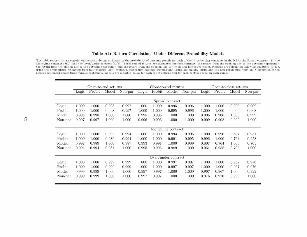
Table A1: Return Correlations Under Different Probability Models

The table reports return correlations across different estimates of the probability of outcome payoffs for each of the three betting contracts in the NBA: the Spread contract (S), theMoneyline contract (ML), and the Over/under contract (O/U). Three sets of returns are calculated for each contract: the return from the opening line to the outcome (open:end),the return from the closing line to the outcome (close:end), and the return from the opening line to the closing line (open:close). Returns are calculated following equations (9-13),using the probabilities estimated from four models: logit, probit, a model that assumes winning and losing are equally likely, and the non-parametric function. Correlation of thereturns estimated across these various probability models are reported below for each set of returns and for each contract type on each game.

Open-to-end returns Close-to-end returns Open-to-close returnsLogit Probit Model Non-par Logit Probit Model Non-par Logit Probit Model Non-par

Spread contract

Logit 1.000 1.000 0.998 0.997 1.000 1.000 0.995 0.996 1.000 1.000 0.906 0.909Probit 1.000 1.000 0.998 0.997 1.000 1.000 0.995 0.996 1.000 1.000 0.906 0.908Model 0.998 0.998 1.000 1.000 0.995 0.995 1.000 1.000 0.906 0.906 1.000 0.999Non-par 0.997 0.997 1.000 1.000 0.996 0.996 1.000 1.000 0.909 0.908 0.999 1.000

Moneyline contract

Logit 1.000 1.000 0.992 0.994 1.000 1.000 0.993 0.995 1.000 0.996 0.807 0.951Probit 1.000 1.000 0.989 0.994 1.000 1.000 0.991 0.995 0.996 1.000 0.764 0.958Model 0.992 0.989 1.000 0.987 0.993 0.991 1.000 0.989 0.807 0.764 1.000 0.705Non-par 0.994 0.994 0.987 1.000 0.995 0.995 0.989 1.000 0.951 0.958 0.705 1.000

Over/under contractLogit 1.000 1.000 0.999 0.999 1.000 1.000 0.997 0.997 1.000 1.000 0.967 0.976Probit 1.000 1.000 0.999 0.999 1.000 1.000 0.997 0.997 1.000 1.000 0.967 0.976Model 0.999 0.999 1.000 1.000 0.997 0.997 1.000 1.000 0.967 0.967 1.000 0.999Non-par 0.999 0.999 1.000 1.000 0.997 0.997 1.000 1.000 0.976 0.976 0.999 1.000

62

Table A2: Correlation of Point Returns

Panel A reports return correlations between dollar-denominated returns and point-denominated returns for the Spread contract (S) andthe Over/under contract (O/U) for three sets of returns for each contract: the return from the opening line to the outcome (open:end),the return from the closing line to the outcome (close:end), and the return from the opening line to the closing line (open:close). PanelB reports the correlations among the point-denominated returns across the different contracts and different return horizons. Returnsare calculated following equations (9-13), using the probabilities estimated from the non-parametric specification.

Panel A: Correlation Between Dollar and Point Returns

Spread contract Over/under contract

Correlation(R$open:end, R

pts.open:end) = 0.79 0.79

Correlation(R$close:end, R

pts.close:end) = 0.79 0.79

Correlation(R$open:close, R

pts.open:close) = 0.28 0.26

Panel B: Point Return Correlations

RSopen:end RS

close:end RSopen:close R

O/Uopen:end R

O/Uclose:end R

O/Uopen:close

RSopen:end 1.00 0.99 0.10 -0.01 -0.01 0.01

RSclose:end 1.00 -0.01 -0.01 -0.01 0.01

RSopen:close 1.00 0.00 0.00 0.03

RO/Uopen:end 1.00 0.99 0.13

RO/Uclose:end 1.00 0.01

RO/Uopen:close 1.00

63

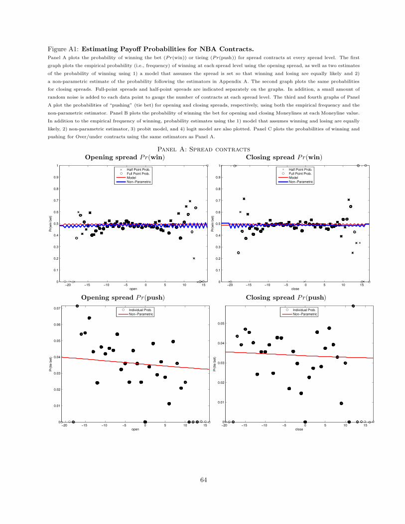
Figure A1: Estimating Payoff Probabilities for NBA Contracts.Panel A plots the probability of winning the bet (Pr(win)) or tieing (Pr(push)) for spread contracts at every spread level. The first

graph plots the empirical probability (i.e., frequency) of winning at each spread level using the opening spread, as well as two estimates

of the probability of winning using 1) a model that assumes the spread is set so that winning and losing are equally likely and 2)

a non-parametric estimate of the probability following the estimators in Appendix A. The second graph plots the same probabilities

for closing spreads. Full-point spreads and half-point spreads are indicated separately on the graphs. In addition, a small amount of

random noise is added to each data point to gauge the number of contracts at each spread level. The third and fourth graphs of Panel

A plot the probabilities of “pushing” (tie bet) for opening and closing spreads, respectively, using both the empirical frequency and the

non-parametric estimator. Panel B plots the probability of winning the bet for opening and closing Moneylines at each Moneyline value.

In addition to the empirical frequency of winning, probability estimates using the 1) model that assumes winning and losing are equally

likely, 2) non-parametric estimator, 3) probit model, and 4) logit model are also plotted. Panel C plots the probabilities of winning and

pushing for Over/under contracts using the same estimators as Panel A.

Panel A: Spread contractsOpening spread Pr(win) Closing spread Pr(win)

−20 −15 −10 −5 0 5 10 150

0.1

0.2

0.3

0.4

0.5

0.6

0.7

0.8

0.9

1

Pr(

win

bet)

open

Half Point Prob.

Full Point Prob.

Model

Non−Parametric

−20 −15 −10 −5 0 5 10 150

0.1

0.2

0.3

0.4

0.5

0.6

0.7

0.8

0.9

1

Pr(

win

bet)

close

Half Point Prob.

Full Point Prob.

Model

Non−Parametric

Opening spread Pr(push) Closing spread Pr(push)

−20 −15 −10 −5 0 5 10 150

0.01

0.02

0.03

0.04

0.05

0.06

0.07

Pr(

tie b

et)

open

Individual Prob.

Non−Parametric

−20 −15 −10 −5 0 5 10 150

0.01

0.02

0.03

0.04

0.05

Pr(

tie b

et)

close

Individual Prob.

Non−Parametric

64

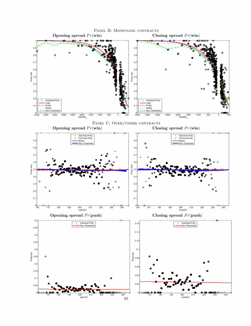
Panel B: Moneyline contractsOpening spread Pr(win) Closing spread Pr(win)

−4500 −4000 −3500 −3000 −2500 −2000 −1500 −1000 −500 0 5000

0.1

0.2

0.3

0.4

0.5

0.6

0.7

0.8

0.9

1

Pr(

win

be

t)

openMLH

Individual Prob.

Logit

Probit

Model

Non−Parametric

−4000 −3500 −3000 −2500 −2000 −1500 −1000 −500 0 5000

0.1

0.2

0.3

0.4

0.5

0.6

0.7

0.8

0.9

1

Pr(

win

be

t)

closeMLH

Individual Prob.

Logit

Probit

Model

Non−Parametric

Panel C: Over/under contractsOpening spread Pr(win) Closing spread Pr(win)

160 170 180 190 200 210 220 230 2400

0.1

0.2

0.3

0.4

0.5

0.6

0.7

0.8

0.9

1

Pr(

win

bet)

openOU

Half Point Prob.

Full Point Prob.

Model

Non−Parametric

160 170 180 190 200 210 220 230 2400

0.1

0.2

0.3

0.4

0.5

0.6

0.7

0.8

0.9

1P

r(w

in b

et)

closeOU

Half Point Prob.

Full Point Prob.

Model

Non−Parametric

Opening spread Pr(push) Closing spread Pr(push)

170 180 190 200 210 220 230 2400

0.05

0.1

0.15

0.2

0.25

0.3

0.35

0.4

0.45

0.5

Pr(

tie b

et)

openOU

Individual Prob.

Non−Parametric

170 180 190 200 210 220 230 2400

0.02

0.04

0.06

0.08

0.1

0.12

0.14

0.16

Pr(

tie b

et)

closeOU

Individual Prob.

Non−Parametric

65

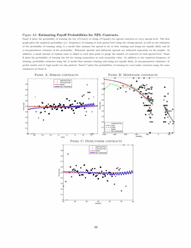
Figure A2: Estimating Payoff Probabilities for NFL Contracts.Panel A plots the probability of winning the bet (Pr(win)) or tieing (Pr(push)) for spread contracts at every spread level. The first

graph plots the empirical probability (i.e., frequency) of winning at each spread level using the closing spread, as well as two estimates

of the probability of winning using 1) a model that assumes the spread is set so that winning and losing are equally likely and 2)

a non-parametric estimate of the probability. Full-point spreads and half-point spreads are indicated separately on the graphs. In

addition, a small amount of random noise is added to each data point to gauge the number of contracts at each spread level. Panel

B plots the probability of winning the bet for closing moneylines at each moneyline value. In addition to the empirical frequency of

winning, probability estimates using the 1) model that assumes winning and losing are equally likely, 2) non-parametric estimator, 3)

probit model, and 4) logit model are also plotted. Panel C plots the probabilities of winning for over/under contracts using the same

estimators as Panel A.

Panel A: Spread contracts Panel B: Moneyline contracts

−20 −15 −10 −5 0 5 10 150

0.1

0.2

0.3

0.4

0.5

0.6

0.7

0.8

0.9

Pr(

win

bet)

close

Half Point Prob.

Full Point Prob.

Model

Non−Parametric

−1000 −800 −600 −400 −200 0 2000

0.1

0.2

0.3

0.4

0.5

0.6

0.7

0.8

0.9

1

Pr(

win

bet)

closeMLH

Individual Prob.

Logit

Probit

Model

Non−Parametric

Panel C: Over/under contracts

30 35 40 45 50 55 600

0.1

0.2

0.3

0.4

0.5

0.6

0.7

0.8

0.9

1

Pr(

win

bet)

closeOU

Half Point Prob.

Full Point Prob.

Model

Non−Parametric

66

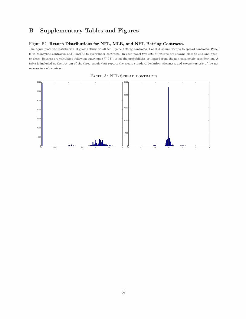
B Supplementary Tables and Figures

Figure B2: Return Distributions for NFL, MLB, and NHL Betting Contracts.The figure plots the distribution of gross returns to all NFL game betting contracts. Panel A shows returns to spread contracts, Panel

B to Moneyline contracts, and Panel C to over/under contracts. In each panel two sets of returns are shown: close-to-end and open-

to-close. Returns are calculated following equations (??-??), using the probabilities estimated from the non-parametric specification. A

table is included at the bottom of the three panels that reports the mean, standard deviation, skewness, and excess kurtosis of the net

returns to each contract.

Panel A: NFL Spread contracts

Close-to-end returns Open-to-close returns

−1 −0.5 0 0.5 1 1.5 20

500

1000

1500

2000

2500

3000

3500

−3 −2 −1 0 1 2 30

500

1000

1500

2000

2500

67

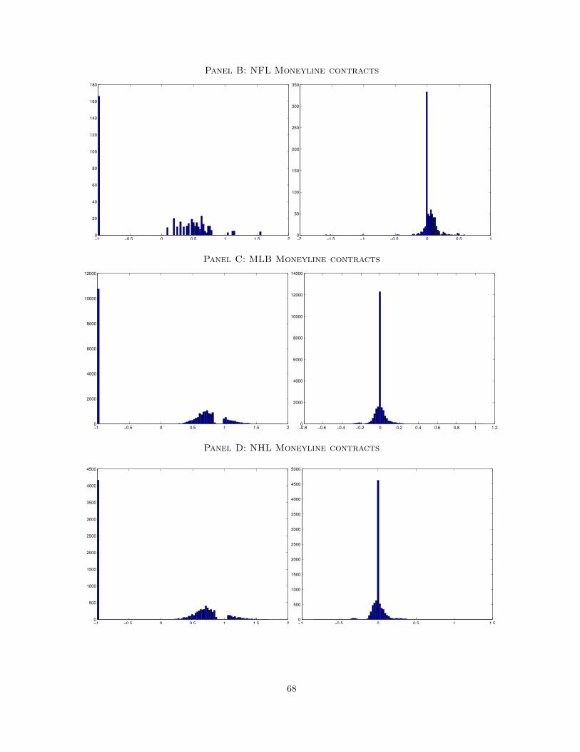
Panel B: NFL Moneyline contracts

Close-to-end returns Open-to-close returns

−1 −0.5 0 0.5 1 1.5 20

20

40

60

80

100

120

140

160

180

−2 −1.5 −1 −0.5 0 0.5 10

50

100

150

200

250

300

350

Panel C: MLB Moneyline contracts

Close-to-end returns Open-to-close returns

−1 −0.5 0 0.5 1 1.5 20

2000

4000

6000

8000

10000

12000

−0.8 −0.6 −0.4 −0.2 0 0.2 0.4 0.6 0.8 1 1.20

2000

4000

6000

8000

10000

12000

14000

Panel D: NHL Moneyline contracts

Close-to-end returns Open-to-close returns

−1 −0.5 0 0.5 1 1.5 20

500

1000

1500

2000

2500

3000

3500

4000

4500

−1 −0.5 0 0.5 1 1.50

500

1000

1500

2000

2500

3000

3500

4000

4500

5000

68

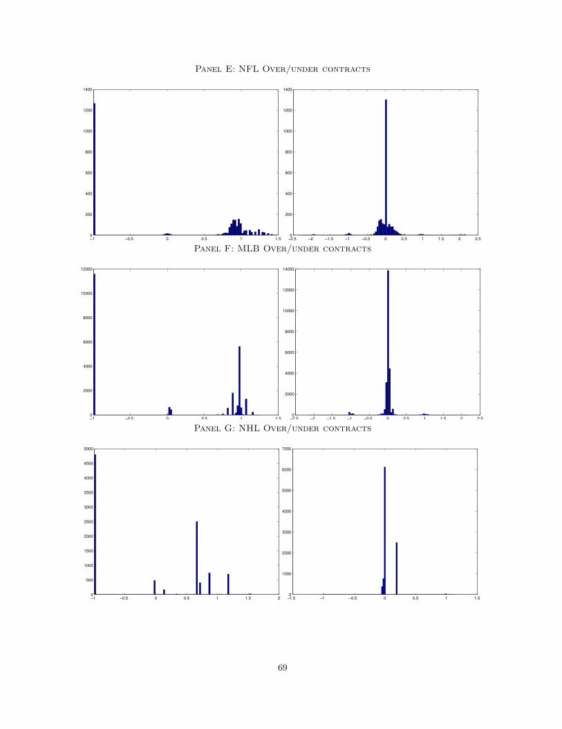
Panel E: NFL Over/under contracts

Close-to-end returns Open-to-close returns

−1 −0.5 0 0.5 1 1.50

200

400

600

800

1000

1200

1400

−2.5 −2 −1.5 −1 −0.5 0 0.5 1 1.5 2 2.50

200

400

600

800

1000

1200

1400

Panel F: MLB Over/under contracts

Close-to-end returns Open-to-close returns

−1 −0.5 0 0.5 1 1.50

2000

4000

6000

8000

10000

12000

−2.5 −2 −1.5 −1 −0.5 0 0.5 1 1.5 2 2.50

2000

4000

6000

8000

10000

12000

14000

Panel G: NHL Over/under contracts

Close-to-end returns Open-to-close returns

−1 −0.5 0 0.5 1 1.5 20

500

1000

1500

2000

2500

3000

3500

4000

4500

5000

−1.5 −1 −0.5 0 0.5 1 1.50

1000

2000

3000

4000

5000

6000

7000

69

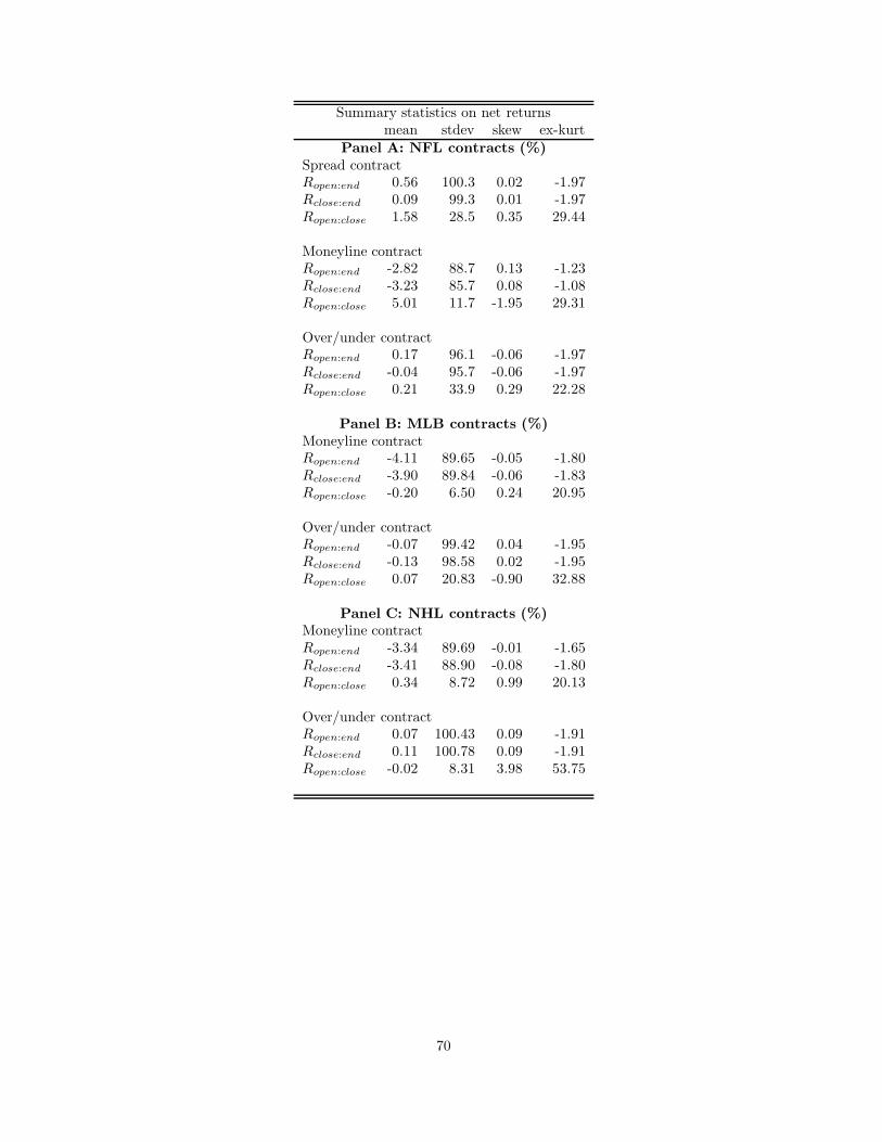
Summary statistics on net returnsmean stdev skew ex-kurt

Panel A: NFL contracts (%)Spread contractRopen:end 0.56 100.3 0.02 -1.97Rclose:end 0.09 99.3 0.01 -1.97Ropen:close 1.58 28.5 0.35 29.44

Moneyline contractRopen:end -2.82 88.7 0.13 -1.23Rclose:end -3.23 85.7 0.08 -1.08Ropen:close 5.01 11.7 -1.95 29.31

Over/under contractRopen:end 0.17 96.1 -0.06 -1.97Rclose:end -0.04 95.7 -0.06 -1.97Ropen:close 0.21 33.9 0.29 22.28

Panel B: MLB contracts (%)Moneyline contractRopen:end -4.11 89.65 -0.05 -1.80Rclose:end -3.90 89.84 -0.06 -1.83Ropen:close -0.20 6.50 0.24 20.95

Over/under contractRopen:end -0.07 99.42 0.04 -1.95Rclose:end -0.13 98.58 0.02 -1.95Ropen:close 0.07 20.83 -0.90 32.88

Panel C: NHL contracts (%)Moneyline contractRopen:end -3.34 89.69 -0.01 -1.65Rclose:end -3.41 88.90 -0.08 -1.80Ropen:close 0.34 8.72 0.99 20.13

Over/under contractRopen:end 0.07 100.43 0.09 -1.91Rclose:end 0.11 100.78 0.09 -1.91Ropen:close -0.02 8.31 3.98 53.75

70

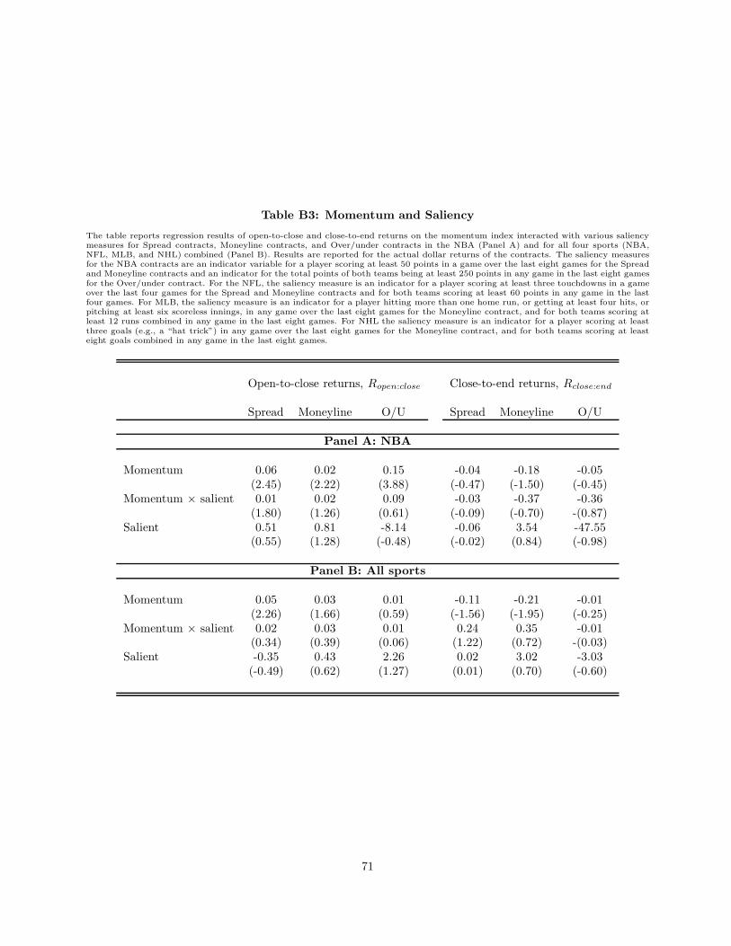
Table B3: Momentum and Saliency

The table reports regression results of open-to-close and close-to-end returns on the momentum index interacted with various saliencymeasures for Spread contracts, Moneyline contracts, and Over/under contracts in the NBA (Panel A) and for all four sports (NBA,NFL, MLB, and NHL) combined (Panel B). Results are reported for the actual dollar returns of the contracts. The saliency measuresfor the NBA contracts are an indicator variable for a player scoring at least 50 points in a game over the last eight games for the Spreadand Moneyline contracts and an indicator for the total points of both teams being at least 250 points in any game in the last eight gamesfor the Over/under contract. For the NFL, the saliency measure is an indicator for a player scoring at least three touchdowns in a gameover the last four games for the Spread and Moneyline contracts and for both teams scoring at least 60 points in any game in the lastfour games. For MLB, the saliency measure is an indicator for a player hitting more than one home run, or getting at least four hits, orpitching at least six scoreless innings, in any game over the last eight games for the Moneyline contract, and for both teams scoring atleast 12 runs combined in any game in the last eight games. For NHL the saliency measure is an indicator for a player scoring at leastthree goals (e.g., a “hat trick”) in any game over the last eight games for the Moneyline contract, and for both teams scoring at leasteight goals combined in any game in the last eight games.

Open-to-close returns, Ropen:close Close-to-end returns, Rclose:end

Spread Moneyline O/U Spread Moneyline O/U

Panel A: NBA

Momentum 0.06 0.02 0.15 -0.04 -0.18 -0.05(2.45) (2.22) (3.88) (-0.47) (-1.50) (-0.45)

Momentum × salient 0.01 0.02 0.09 -0.03 -0.37 -0.36(1.80) (1.26) (0.61) (-0.09) (-0.70) -(0.87)

Salient 0.51 0.81 -8.14 -0.06 3.54 -47.55(0.55) (1.28) (-0.48) (-0.02) (0.84) (-0.98)

Panel B: All sports

Momentum 0.05 0.03 0.01 -0.11 -0.21 -0.01(2.26) (1.66) (0.59) (-1.56) (-1.95) (-0.25)

Momentum × salient 0.02 0.03 0.01 0.24 0.35 -0.01(0.34) (0.39) (0.06) (1.22) (0.72) -(0.03)

Salient -0.35 0.43 2.26 0.02 3.02 -3.03(-0.49) (0.62) (1.27) (0.01) (0.70) (-0.60)

71

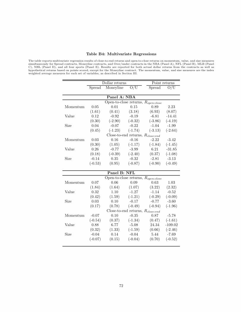
Table B4: Multivariate Regressions

The table reports multivariate regression results of close-to-end returns and open-to-close returns on momentum, value, and size measuressimultaneously for Spread contracts, Moneyline contracts, and Over/under contracts in the NBA (Panel A), NFL (Panel B), MLB (PanelC), NHL (Panel D), and all four sports (Panel E). Results are reported for both actual dollar returns from the contracts as well ashypothetical returns based on points scored, except for the Moneyline contract. The momentum, value, and size measures are the indexweighted average measures for each set of variables, as described in Section III.

Dollar returns Point returnsSpread Moneyline O/U Spread O/U

Panel A: NBA

Open-to-close returns, Ropen:close

Momentum 0.05 0.01 0.15 0.89 2.23(1.61) (0.41) (3.18) (6.93) (8.07)

Value 0.12 -0.92 -0.19 -6.81 -14.41(0.30) (-2.90) (-0.32) (-3.86) (-4.19)

Size 0.04 -0.07 -0.22 -1.04 -1.99(0.45) (-1.23) (-1.74) (-3.13) (-2.64)

Close-to-end returns, Rclose:end

Momentum 0.03 0.16 -0.16 -2.22 -3.42(0.30) (1.05) (-1.17) (-1.84) (-1.45)

Value 0.26 -0.77 -3.99 6.21 -31.85(0.18) (-0.39) (-2.40) (0.37) (-1.08)

Size -0.14 0.35 -0.32 -2.81 -3.13(-0.53) (0.95) (-0.87) (-0.90) (-0.49)

Panel B: NFLOpen-to-close returns, Ropen:close

Momentum 0.07 0.06 0.09 0.63 1.03(1.84) (1.64) (1.07) (3.22) (2.32)

Value 0.32 1.10 -1.27 -1.14 -0.52(0.42) (1.59) (-1.21) (-0.29) (-0.09)

Size 0.03 0.10 -0.17 -0.77 -3.60(0.17) (0.78) (-0.49) (-0.94) (-1.96)

Close-to-end returns, Rclose:end

Momentum -0.07 0.10 -0.35 0.87 -5.78(-0.54) (0.37) (-1.34) (0.47) (-1.61)

Value 0.88 6.77 -5.08 24.34 -109.02(0.32) (1.33) (-1.59) (0.66) (-2.46)

Size -0.04 0.14 -0.04 5.44 -7.69(-0.07) (0.15) (-0.04) (0.70) (-0.52)

72

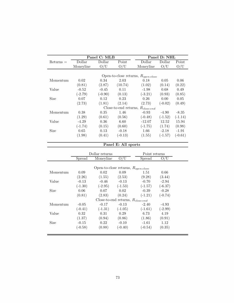
Panel C: MLB Panel D: NHLReturns = Dollar Dollar Point Dollar Dollar Point

Moneyline O/U O/U Moneyline O/U O/U

Open-to-close returns, Ropen:close

Momentum 0.02 0.34 2.03 0.18 0.05 0.06(0.81) (2.87) (10.74) (1.02) (0.14) (0.22)

Value -0.52 -0.45 0.11 -1.98 0.68 0.49(-2.79) (-0.90) (0.13) (-3.21) (0.93) (0.85)

Size 0.07 0.12 0.23 0.26 0.00 0.05(2.73) (1.81) (2.14) (2.73) (-0.02) (0.49)

Close-to-end returns, Rclose:end

Momentum 0.38 0.35 1.46 -0.93 -4.90 -8.35(1.29) (0.61) (0.56) (-0.48) (-1.52) (-1.14)

Value -4.29 0.36 6.60 -12.07 12.52 15.94(-1.74) (0.15) (0.60) (-1.75) (1.74) (0.98)

Size 0.65 0.13 -0.18 1.66 -2.18 -1.91(1.98) (0.41) (-0.13) (1.55) (-1.57) (-0.61)

Panel E: All sports

Dollar returns Point returnsSpread Moneyline O/U Spread O/U

Open-to-close returns, Ropen:close

Momentum 0.09 0.02 0.09 1.51 0.66(2.26) (1.55) (2.53) (9.28) (3.44)

Value -0.13 -0.46 -0.13 -0.70 -2.94(-1.30) (-2.95) (-1.53) (-1.57) (-6.37)

Size 0.06 0.07 0.02 -0.39 -0.28(0.81) (2.83) (0.24) (-1.21) (-0.74)

Close-to-end returns, Rclose:end

Momentum -0.05 -0.17 -0.13 -2.40 -4.93(-0.41) (-1.31) (-1.05) (-1.61) (-2.99)

Value 0.32 0.31 0.29 6.73 4.19(1.37) (0.94) (0.86) (1.86) (0.91)

Size -0.15 0.22 -0.10 -1.61 1.12(-0.58) (0.88) (-0.40) (-0.54) (0.35)

73

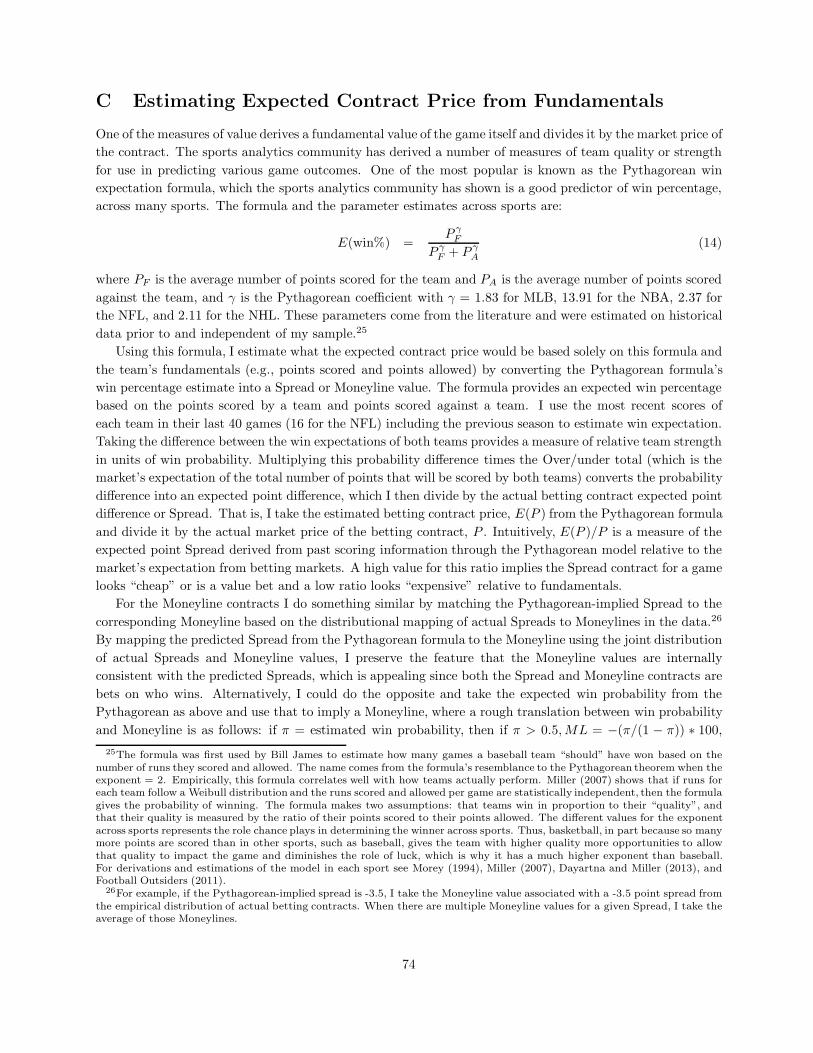
C Estimating Expected Contract Price from Fundamentals

One of the measures of value derives a fundamental value of the game itself and divides it by the market price of

the contract. The sports analytics community has derived a number of measures of team quality or strength

for use in predicting various game outcomes. One of the most popular is known as the Pythagorean win

expectation formula, which the sports analytics community has shown is a good predictor of win percentage,

across many sports. The formula and the parameter estimates across sports are:

E(win%) =P γ

F

P γF + P γ

A

(14)

where PF is the average number of points scored for the team and PA is the average number of points scored

against the team, and γ is the Pythagorean coefficient with γ = 1.83 for MLB, 13.91 for the NBA, 2.37 for

the NFL, and 2.11 for the NHL. These parameters come from the literature and were estimated on historical

data prior to and independent of my sample.25

Using this formula, I estimate what the expected contract price would be based solely on this formula and

the team’s fundamentals (e.g., points scored and points allowed) by converting the Pythagorean formula’s

win percentage estimate into a Spread or Moneyline value. The formula provides an expected win percentage

based on the points scored by a team and points scored against a team. I use the most recent scores of

each team in their last 40 games (16 for the NFL) including the previous season to estimate win expectation.

Taking the difference between the win expectations of both teams provides a measure of relative team strength

in units of win probability. Multiplying this probability difference times the Over/under total (which is the

market’s expectation of the total number of points that will be scored by both teams) converts the probability

difference into an expected point difference, which I then divide by the actual betting contract expected point

difference or Spread. That is, I take the estimated betting contract price, E(P ) from the Pythagorean formula

and divide it by the actual market price of the betting contract, P . Intuitively, E(P )/P is a measure of the

expected point Spread derived from past scoring information through the Pythagorean model relative to the

market’s expectation from betting markets. A high value for this ratio implies the Spread contract for a game

looks “cheap” or is a value bet and a low ratio looks “expensive” relative to fundamentals.

For the Moneyline contracts I do something similar by matching the Pythagorean-implied Spread to the

corresponding Moneyline based on the distributional mapping of actual Spreads to Moneylines in the data.26

By mapping the predicted Spread from the Pythagorean formula to the Moneyline using the joint distribution

of actual Spreads and Moneyline values, I preserve the feature that the Moneyline values are internally

consistent with the predicted Spreads, which is appealing since both the Spread and Moneyline contracts are

bets on who wins. Alternatively, I could do the opposite and take the expected win probability from the

Pythagorean as above and use that to imply a Moneyline, where a rough translation between win probability

and Moneyline is as follows: if π = estimated win probability, then if π > 0.5, ML = −(π/(1 − π)) ∗ 100,

25The formula was first used by Bill James to estimate how many games a baseball team “should” have won based on thenumber of runs they scored and allowed. The name comes from the formula’s resemblance to the Pythagorean theorem when theexponent = 2. Empirically, this formula correlates well with how teams actually perform. Miller (2007) shows that if runs foreach team follow a Weibull distribution and the runs scored and allowed per game are statistically independent, then the formulagives the probability of winning. The formula makes two assumptions: that teams win in proportion to their “quality”, andthat their quality is measured by the ratio of their points scored to their points allowed. The different values for the exponentacross sports represents the role chance plays in determining the winner across sports. Thus, basketball, in part because so manymore points are scored than in other sports, such as baseball, gives the team with higher quality more opportunities to allowthat quality to impact the game and diminishes the role of luck, which is why it has a much higher exponent than baseball.For derivations and estimations of the model in each sport see Morey (1994), Miller (2007), Dayartna and Miller (2013), andFootball Outsiders (2011).

26For example, if the Pythagorean-implied spread is -3.5, I take the Moneyline value associated with a -3.5 point spread fromthe empirical distribution of actual betting contracts. When there are multiple Moneyline values for a given Spread, I take theaverage of those Moneylines.

74

or if π < 0.5, ML = (1 − π)/(π) ∗ 100. Then, taking the Moneyline estimated from the Pythagorean win

probability, I could match the Moneyline to a Spread using the empirical distribution of Moneylines and

Spreads to also make the estimates internally consistent. Both methods of computing expected Spreads and

Moneylines yield nearly identical results.

For Over/under contracts, which are bets on total points scored by both teams combined, I run a rolling

regression model of O/U totals on points scored by the home team, points scored against the home team,

points scored by visiting team, and points scored against visiting team over the last 40 games (16 games in

the NFL) for each team. Using the regression coefficients for both teams, I then apply them to the average

points scored for and against for each team over the last 40 games (16 games in the NFL) and then take an

average of the predicted point totals for the two teams, which represents a predicted O/U point total from

the number of points scored for and against each team over the last 40 games. This predicted point total is

then divided by the actual O/U total from the betting market to obtain a value measure. Alternatively, I

could have taken a moving average O/U total from betting markets over the past 40 games involving either

team and taken the average across the two teams for my fundamental O/U total. Using this measure instead,

I get very similar results.

To estimate the residual value measure, I estimate the expected price of the contract by running a rolling

regression each season of the betting line on team × home and team × away dummy variables, a variable

representing the number of games played in the last three days, a variable representing if the visiting team

is playing its second consecutive game away from home, and cumulative points scored for and against both

teams. The regression requires a minimum of 20 games per team and hence only examines contracts beginning

with the 21st game each season. Using the slope coefficients from this regression, I then forecast the betting

line (Spread, Moneyline, or Over/under) on the next game and take the difference between the actual betting

line and this forecast as the residual value measure. The predicted regressions based on the above observables

have an R2 of 0.80 on average, indicating that this simple model can predict a significant component of these

betting lines. This measure of value changes at a much higher frequency than those above and captures very

short-term deviations from expected betting lines.

75