EE225E/BIOE265 Spring 2013 Miki LustigPrinciples of MRI

Assignment 6 Solutions

Due March 15, 2013

1. Read Nishimura Ch. 6

2. Nishimura assignment 6.5

Solution:This question demonstrates a very cool way of storing encoding information in Mz. The advantagein storing information in the longitudal direction is the long relaxation time of T1, which is usuallymuch longer than T2. This way, encoded information can be stored for long time periods beforedecoded.

Since we ignore relaxation, the solution of the Bloch equation is a series of rotations. The first RFpulse produces a 90◦ degree rotation around the x axis pulse. The z gradient produces a z dependentrotation around the z axis, α = γGzzT . Finally, the 2nd RF pulse produces a −90◦ degree rotationaround the x axis. The series of rotations is:

M = Rx(−90)Rz(γGzzT )Rx(90)M0

So, if the magnetization starts at M0 = [0, 0,Mz0]T then after the first RF we get, 1 0 0

0 0 10 −1 0

0

0Mz0

=

0Mz0

0

.After the gradient we get, cos(γGzzT ) sin(γGzzT ) 0

− sin(γGzzT ) cos(γGzzT ) 00 0 1

0Mz0

0

=

Mz0 sin(γGzzT )Mz0 cos(γGzzT )

0

.After the final RF we get, 1 0 0

0 0 −10 1 0

Mz0 sin(γGzzT )Mz0 cos(γGzzT )

0

=

Mz0 sin(γGzzT )0

Mz0 cos(γGzzT )

.So, Mz is cosine modulated in z. This is in fact encoding the real part of a phase-encode in Mz!

Here is a SpinBench simulation plot, where the gradient produced a phase of 10 cycles/cm (γGzT =10)

ZPosition (mm)-4 -2 0 2 4

Mz

Time

Gx

Gy

Gz

RF

10 cycles/cm

1

3. Mimimum-Phase RF Excitation

a) We would like to use the waveform plotted below as an RF excitation pulse. Assume that theslice select gradient is applied during the pulse, and then inverted to refocus the slice. What isthe duration of the refocusing gradient that produces the maximum signal?

Solution: The refocusing gradient basically takes us backwards in time through the excitationpulse. If the refucusing gradient and the slice select gradient have the same amplitude, thenrefocusing by t ms takes us to a point t ms before the end of the pulse. The signal we receive isproportional to the amplitude of the pulse at that time.

In this case, the largest signal corresponds to a time of 3.1 ms during the pulse, or 0.9 ms fromthe end of the pulse. Hence a refocusing interval of 0.9 ms produces the maximum signal.

b) If we refocus for 2 ms, which is 1/2 the slice select gradient length, how does the signal compareto that of part (a)?

Solution: If we refocus for 2 ms, this will bring us to the t = 2 ms point in the RF pulse,where the k-space weighting is zero. This refocusing interval produces no signal, which is muchsmaller than the answer for (a).

0 0.5 1 1.5 2 2.5 3 3.5 4

−0.01

0

0.01

0.02

0.03

Time, ms

B1(

t), G

2

4. From Midterm I 2011: RF Excitation and Excitation k-space

For each of the following selective excitations, find (qualitatively) the associated excitation k-spaceand the magnitude of the slice profile at the end of the pulse, e.g., |Mxy(z, T )|. Draw them qualita-tively, pointing out the “interesting” parts. Assume small tip-angle approximation.

a) What do these pulses do?

B1

Gz

Solutions:The pulse deposits two windowed sinc B1 pulses next to each other in excitation k-space. Thepulses are not symmetric around kz = 0, but this only affects the phase of the Mxy profile, notthe magnitude!

If the length of the wsinc is T in k-space then the its k-space expression is

B1(kz) = W (kz)sinc(kz) ∗ (δ(kz) + δ(kz − T ))

= 2W (kz)sinc(kz) ∗(δ(kz + T/2) + δ(kz − T/2)

2

)∗ δ(kz + T/2)

The slice profile is the Fourier transform of the above,

Mxy = F{B1(kz)}(z) = 2(w(z) ∗ u(z)) cos

(2πT

2z

)ei2π

T2z.

When we take the magnitude, we lose the linear phase component,

|Mxy| =∣∣∣∣2(w(z) ∗ u(z)) cos

(2πT

2z

)∣∣∣∣Which is a cosine modulated slice profile.

B1 |Mxy|

Kz z

3

b) What do these pulses do?

B1

Gz

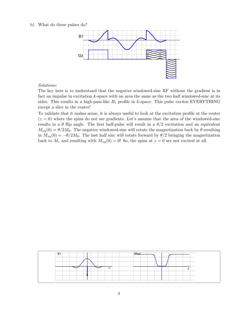
Solutions:The key here is to understand that the negative windowed-sinc RF without the gradient is infact an impulse in excitation k-space with an area the same as the two half windowed-sinc at itssides. This results in a high-pass-like B1 profile in k-space. This pulse excites EVERYTHINGexcept a slice in the center!

To validate that it makes sense, it is always useful to look at the excitation profile at the center(z = 0) where the spins do not see gradients. Let’s assume that the area of the windowed-sincresults in a θ flip angle. The first half-pulse will result in a θ/2 excitation and an equivalentMxy(0) = θ/2M0. The negative windowed-sinc will rotate the magnetization back by θ resultingin Mxy(0) = −θ/2M0. The last half sinc will rotate forward by θ/2 bringing the magnetizationback to Mz and resulting with Mxy(0) = 0! So, the spins at z = 0 are not excited at all.

B1 |Mxy|

Kz z

4

c) What do these pulses do?

B1

Gz

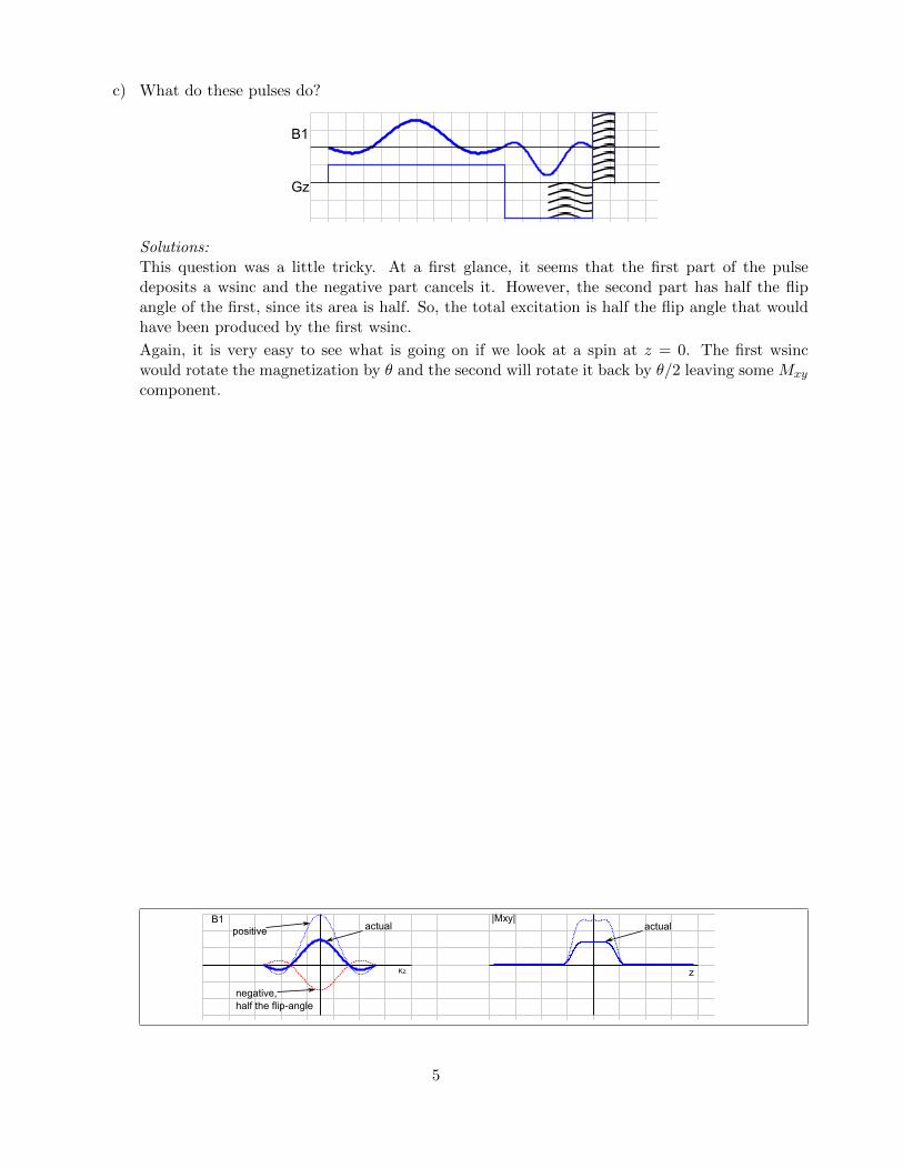
Solutions:This question was a little tricky. At a first glance, it seems that the first part of the pulsedeposits a wsinc and the negative part cancels it. However, the second part has half the flipangle of the first, since its area is half. So, the total excitation is half the flip angle that wouldhave been produced by the first wsinc.

Again, it is very easy to see what is going on if we look at a spin at z = 0. The first wsincwould rotate the magnetization by θ and the second will rotate it back by θ/2 leaving some Mxy

component.

B1 |Mxy|

Kz z

actualpositive

negative, half the flip-angle

actual

5

5. In this problem we will determine the excitation profile of the following pulse, below on the left,

Δkz = 1 cycle/cm

RF

Gz

0 2 4 6 8 t, ms 0 1 2 4 6 8 t, ms

a(t)

This is a small-tip-angle pulse. The RF and gradient are applied alternately. One lobe of the gradientproduces a change in kz of

∆kz =γ

2π

∫ 1

0G(τ)dτ = 1 cycle/cm

The area of each RF subpulse corresponds to a sample of a TBW = 4 windowed sinc shown aboveon the right.

a) Plot the magnitude of the spectrum A(f) of the sampled windowed sinc. You do not have tocompute an expression. Label the axes of the plot.

Solution:

The signal a(t) is a sampled TBW=4 windowed sinc. It is sampled at 1 kHz (1 ms samples) sothe spectrum A(f) is periodic with period 1 kHz. Since (T )(BW ) = 4, and the duration of thepulse is 8 ms, the width of the passband is

BW = 4/8 ms = 0.5 kHz

or ±0.25kHz. The transition width is about 2/T = 2/8 ms = 0.25 kHz. The spectrum |A(f)|then looks like:

|A( f )|

f , kHz0 1 2-1-2

· · ·· · ·500 Hz

6

b) Plot the k-space weighting that the RF pulse produces.

Solution:

The RF and gradient are applied alternately. The gradient lobes produce a step in kz of 1cycle/cm. Each RF pulse is applied at one discrete kz (the gradient is off during the RF), soeach RF subpulse produces an impulse in k-space, each with a strength determined by the area,or flip angle, of each subpulse. The k-space variable is the integral of the remaining gradient,so it starts a 8 cycles/cm, and moves to the left with 1 cycle/cm steps, ending a kz = 0.

The k-space weighting is then

γB1(t) vs k(t)

kz, cycles/cm0 4 8-4-8

c) Plot the magnitude of the magnetization |Mxy(z)| produced by the RF pulse.

Hint: Appoximate the RF pulse as an ideal sampled pulse as in (a) with a constant gradient.

Solution:

The Mxy(z) is the Fourier transform of the function plotted in (b). However, this looks just likea(t), so |Mxy(z) should look like your answer in (a), but will be a function of space, cm, insteadof frequency, kHz. We only need to identify the scale factor.

The simplest approach is to notethat the k-space weighting is discretely sampled, with ∆kz = 1cycle/cm, which means that |Mxy(z)| is periodic with period 1 cm. Referring to (a), 1 cm willcorrespond to 1 kHz, and the magnetization profile will look like:

|Mxy(z)|

z, cm0 1 2-1-2

· · ·· · ·0.5 cm

7

6. Relaxation During RF Pulses (From Midterm II 2012)

When deriving the small-tip-angle approximation for slice selective RF pulses we assumed that theRF pulse duration is much smaller than T2, and so it can be neglected. This is a good approximationin general, but fails when the T2 relaxation is short. In this question we will explore the case whenT2 relaxation can not be neglected anymore. We will still assume the small-tip-angle approximationin which Mz = M0 for the entire pulse duration. Under this approximation, at each time point newtransverse magnetization is created and evolves independently. For example, consider the followingpulse

B1

Gz

t=TG

t=t1t=0

TheB1 field at time t = t1 will produce new transverse magnetization ∆Mxy(z, t1) = iM0 sin(γB1(t1)∆t) ≈iM0γB1(t1)∆t

a) The new x-verse magnetization ∆Mxy(z, t1) will evolve over time. Find an expression for it atthe end of the pulse (at time T). Assume transverse relaxation T2.

Solutions:

The magnetization will exhibit precession due to the remaining gradient e−iγ∫ Tt1Gz(τ)dτ

and

decay e−T−t1

T2 due to the transverse relaxation.

∆Mxy(z, t1) at time T = iM0(γB1(t1)∆t)e−T−t1

T2 e−iγ∫ Tt1Gz(τ)dτ

8

b) Show that the slice profile Mxy(z, T ) has the form of

Mxy(z, T ) = iγM0

∫ T

0B̃1(t)e

−i2πkz(t)zdt

Find the expression for the ”effective RF field” B̃1(t) as a function of the original B1(t). Whatis kz(t)?

Solutions:

First, in the same way as derived in class, we can define kz(t) = γ2π

∫ Tt Gz(τ)dτ . That is, k-space

is the area of the remaining gradient waveform. The transverse relaxation we can bundle with

the B1 field to get B̃1(t) = B1(t)e−T−t

T2 . This means that the effective B1 field is weighted byan exponential decay from the end of the pulse.

B̃1(t) = B1(t)e−T−t

T2 kz(t) = γ2π

∫ Tt Gz(τ)dτ

c) The slice profile can be expressed as a Fourier transform in excitation k-space

Mxy(z, T ) = iγM0

∫kzB̃1(kz)e

−i2πkzzdkz.

For the above pulse, find the expression for t as a function of kz, then find the “effective” RFfield in k-space B̃1(kz).

B̃1(kz) has the form: B̃1(kz) = C ·W (kz)B1(kz) where C is a constant and W (kz) is a functionof kz)

Solutions:

We first need to express t as a function of kz.

kz(t) =γ

2π

∫ T

tGz(τ)dτ

=γ

2πG · (t1 − t)

So,

t = − kzγ2πG

+ t1

and,

B̃1(kz) = B1(kz)e−T−t1

T2 e− kz

γ2πGT2 .

B̃1(kz) = B1(kz)e−T−t1

T2 e− kz

γ2πGT2

9

d) What will be the (two) effects of T2 relaxation on the actual slice profile? Explain.

Solutions:

There are two effects, the dominant one is just bulk scaling of the B1 due to the decay from the

middle of the RF till the end of the pulse e−T−t1

T2 . The other is a k-space weighting e− kz

γ2πGT2

that will cause a blurring of the slice profile.

Effect I: A lower flip angle of e−T−t1

T2 due to the relaxation from the middle of the RF till theend of the pulse

Effect II : An excitation k-space weighting e− kz

γ2πGT2 that will cause a blurring of the slice profile

with the inverse Fourier transform of the weighting.

e) The T2 of white matter is two orders of magnitude longer than the T2 of myelin. Design(qualitatively) a slice selective RF pulse that will mostly excite myelin.

Solutions:

There are many options here. The main point is that the RF for the excitation k-space of thelong T2 should integrate to zero, whereas for the short T2 due to decay it will not integrate tozero.

B1

Gz

7. Design the following slice-selective excitation pulses. In each case, choose a time-bandwidth productthat is a multiple of four. The maximum gradient strength is 4 G/cm. Assume the excitation pulseis a Hamming windowed sinc, as we described in class, and that we want the sharpest profile withinthe constraints.

a) Design a pulse to excite a 3 mm slice. The pulse should be 1 ms in duration. Find the time-bandwidth of the pulse, and the amplitude of the slice-select gradient.

Solution: First, the maximum gradient we have is 4 G/cm, or

(4 G/cm)(4.257 kHz/G) = 17 kHz/cm.

A 3 mm slice then has a bandwidth of

(17 kHz/cm)(0.3cm) = 5.1 kHz.

This is the maximum bandwidth that we will ever need with our gradient system.

Next, we need to choose the time-bandwidth of our RF pulse. The maximum time bandwidthis

(1 ms)(5.1 kHz) = 5.1

10

We want this to be a multiple of 4, so we choose a time-bandwidth of 4.

Then the bandwidth isBW = TBW/T = 4/(1 ms) = 4 kHz.

The gradient strength is then found by solving

γ

2πGz∆z = 4 kHz

for Gz. The result is

Gz =4 kHz

( γ2π )(∆z)

=4 kHz

(4.257 kHz/G)(0.3 cm)= 3.13 G/cm.

b) Design a pulse to excite a 8 cm slab. Assume we want to use a time-bandwidth 16 pulse, andthat the shortest time we can play this waveform is 2 ms, due to limits on peak RF amplitude.What is the gradient amplitude?

Solution: We know the time, and the time-bandwidth product, so the bandwidth of the pulseis

BW = TBW/(T ) = 16/(2 ms) = 8 kHz.

We want this to correspond to an 8 cm slab, so

8 kHz. =γ

2πGz∆z = (4.257 kHz/G)Gz(8 cm)

Solving for Gz we getGz = 0.235 G/cm.

c) A 2 ms, time-bandwidth 8 pulse is to be used to excite a 1 cm slice centered at +12 cm fromgradient isocenter (the zero point of the gradients). Find the gradient amplitude for this pulse,and the frequency for the RF pulse compared to the slice at isocenter.

Solution: The bandwidth of this pulse is

BW = 8/(2 ms) = 4 kHz

If this is a 1 cm slice, then

4 kHz =γ

2πGz∆z = (4.257 kHz/G)Gz(1 cm)

Solving for GzGz = 0.94 G/cm.

This corresponds to

γ

2πGz = (4.257 kHz/G)(0.94 G/cm) = 4 kHz/cm.

Hence, in order to offset the slice by 12 cm, we need to increase the frequency of the RFtransmitter by

(4 kHz/cm)(12 cm) = 48 kHz.

11

8. Introduction: This assignment concerns typical Fourier transform designs of excitation pulses. Thisincludes designing windowed sinc pulses, calculating the RF amplitude required, simulating slice pro-files,designing a pulse for a specific application, and computing the relative SAR of a pulse sequence.For simulating the slice profile, you will need the bloch simulator.

a. Design of Windowed Sinc RF Pulses Write an m-file that computes a Hamming windowedsinc pulse, given a time-bandwidth product, and number of samples.

>> rf = wsinc(timebandwidth, samples)

Write the mfile so that it scales the waveform to sum to one, sum(rf) = 1. Plot windowed sincswith TBW of 4, 8, and 12. The TBW=4 pulse is common for 180 degree pulses, the TBW of 8 istypical for excitation pulses, and a TBW of 12 or 16 is typical for slab select pulses.

Solution:

function rf = wsinc(timebandwidth, samples)

%

% rf = wsinc(timebandwidth, samples)

%

% function returns a hamming windowed sinc rf pulse.

% timebandwidth is T*df, for a windowed sinc it is the number of

% zero crossings of the pulse.

%

%

% Although it is probably not important, I made sure that

% the 1st and last samples are not zero.

%

%

% (c) Michael Lustig 2004

theta = [linspace(-timebandwidth/2, timebandwidth/2, samples+2)]’;

rf = sinc(theta(2:end-1)).*hann(samples);

rf = rf/(sum(rf));

12

0 10 20 30 40 50 60 70 80 90 100−0.05

0

0.05

0.1

0.15

TBW=4TBW=8TBW=12

b. Plot RF Amplitude For convenience, we will assume that the RF waveforms are normalizedso that the sum of the RF waveform is the flip angle in radians. The sampled RF waveform can thenbe thought of as a sequence of small flips. This eliminates the need to explicitly consider the pulseduration in the design and simulation. However, it is sometimes important to compute the RF pulseamplitude in Gauss. In this problem you will write an m-file that takes a normalized RF pulse, andthen, given a overall pulse length, scales the waveform to Gauss.

First, generate a 3.2 ms, TBW = 8 windowed sinc RF pulse, and scale it to a π/2 flip angle

>> rf = (pi/2)* wsinc(8,256);

Then, write an m-file called rfscaleg that takes a normalized RF pulse and a pulse duration, andreturns a waveform that is scaled to Gauss,

>> rfs = rfscaleg(rf, pulseduration);

Plot the pulse you generated, scaled to Gauss. Label the axes. What is the peak amplitude?

Solution: One possible m-file for rfscaleg.m is

function rfs = rfscaleg(rf,t);

% rfs = rfscaleg(rf,t)

%

% rf -- rf waveform, scaled so sum(rf) = flip angle

% t -- duration of RF pulse in ms

% rfs -- rf waveform scaled to Gauss

%

gamma = 2*pi*4.257; % kHz/G

dt = t/length(rf);

rfs = rf/(gamma*dt);

13

This takes the rotation produced by each sample, and determines what RF amplitude would beneeded to produce that rotation in one sample dwell time. Note that the input RF is in radians, sowe need the 2π factor in gamma.

The scaled RF plot looks like

0 0.5 1 1.5 2 2.5 3−0.05

0

0.05

0.1

0.15

Time, ms

Ampl

itude

, Gau

ss

The peak amplitude is a about 0.147 G.

c. Simulated Slice Profiles We will use the bloch simulator for simulating the RF pulse.

Calculate the slice thickness of the TBW = 8 pulse from problem (b), based on the relations presentedin class. Assume the slice select gradient is 0.6 G/cm. Simulate the RF pulse using

> dp = linspace(-2,2,512).’; % simulate from -2cm to 2cm

> mx0 = zeros(512,1); my0=zeros(512,1);, mz0 = ones(512,1);

> dt = 3.2e-3/256;

> [mx,my,mz] = bloch(rfs,g,dt,100,100,0,dp,0,mx0,my0,mz0);

> mxy = mx+i*my;

> figure, plot(dp,abs(mxy)), xlabel(’cm’), ylabel(’amplitude’);

Is the slice the expected width?

Solutions:

The slice width can be found fromT (BW ) = 8

soBW = 8/(3.2 ms) = 2.5 kHz

The gradient strength is 0.6 G/cm or γ2π0.6 G/cm = 2.55 kHz/cm. The slice thickness is then about

2.5 kHz

2.55 kHz/cm= 0.98 cm

14

−2 −1.5 −1 −0.5 0 0.5 1 1.5 2−0.2

0

0.2

0.4

0.6

0.8

1

1.2

position, cm

Ampl

itude

This shows the half-amplitude width to be about 1 cm, very close to what we calculated.

d. Design a Slab Select Pulse You are designing a 3D pulse sequence, and you need a slabselect pulse in the z dimension. You have 6 ms for the pulse, and want it to be as sharp as possible.You also have a peak RF amplitude constraint of 0.17 G.

(a) What is the highest time-bandwidth you can allow, given that the maximum flip angle will be90 degrees?

Solution: Trying a few values we get

>> max(rfscaleg((pi/2)*wsinc(16,256),6))

ans =

0.1572

>> max(rfscaleg((pi/2)*wsinc(17,256),6))

ans =

0.1667

>> max(rfscaleg((pi/2)*wsinc(18,256),6))

ans =

0.1762

So TBW = 17 is OK, and TBW = 18 is not. We could go for more resolution if you want, andcome put with a TBW = 17.35 that is pretty close to 0.17 G, but 16 or 17 is fine.

(b) Assume we want the minimum slab thickness to be 8 cm. What is the gradient amplitude thatthis requires?

Solution: Assuming TBW = 17, and a 6 ms pulse, the frequency bandwidth is

BW =17

6 ms= 2.83 kHz

We want this to be 8 cm, so γ2πG(8 cm) = 2.83 kHz, and

G =2.83 kHz

(4.257 kHz/G)(8 cm)= 0.083 G/cm

15

Your answer will differ, depending on the TBW product you used. The important point to noteis that this is very low, only about 350 Hz/cm. This means that patient susceptibility shifts aregoing to distort the slab.

16

(c) Simulate the slice profile. How wide is the transition band compared to the passband? Assumethat the passband edge is 95% of the middle of the passband, and the stopband edge is 5% ofthe passband.

Solution:

−8 −6 −4 −2 0 2 4 6 80

0.2

0.4

0.6

0.8

1

position, cm

Ampl

itude

3 3.2 3.4 3.6 3.8 4 4.2 4.4 4.6 4.8 50

0.2

0.4

0.6

0.8

1

position, cm

Ampl

itude

The slab thickness is about 8 cm which is what we designed for, and the transition width(neglecting the sidelobe) is about 0.7 cm. We’d expect the transition width to be about 8 cm/(17/2) = 0.94 cm. This is off somewhat, but is due to how exactly the transition width isdefined. It is on the right order, though.

e. Compute the Relative SAR of a Pulse Sequence SAR stands for specific absorption rateand is the amount of RF energy deposition in the body. Usually, this is calculated using softwaremodel that gives the SAR limit measured in terms of 1 ms rectangular 180 degree pulses (“hard”180’s). This depends on the patient weight, body part, and RF coil. The limit might be 100 hard

17

180s per second, for example. The power of a particular RF pulse is

P =

∫B2

1(t) dt.

The relative SAR of a particular RF pulse is it’s power divided by the power in a 1 ms hard 180.The relative SAR of a pulse sequence is computed as the sum of the relative SAR’s of each of thepulses, measured in equivalent hard 180’s.

Write an mfile rsar.m which takes a normalized RF pulse and pulse duration, and returns the relativeSAR, measured in equivalent hard 180’s

>> eq180 = rsar(rf,t)

Assume that you are developing a very fast sequence. The excitation pulse is a 1 ms TBW=2windowed sinc. Assume you need a TR of 2.25 ms. What is the maximum flip angle you can allow,given that the SAR limit is 100 equivalent 180’s per second?

Solution: The samples of the normalized RF pulse are

γB1(ti)∆t

which is the flip angle in radians that each sample produces. What we want to compute is∑i

(γB1(ti))2∆t

and compare this to the value of a hard 180

(γB1)2∆t = π2(1 ms) = π2

An m-file computes this ratio is given below:

function npi = rsar(rf,t)

% npi = rsar(rf,t)

%

% rf -- rf waveform, scaled so that sum(rf) = flip angle

% t -- duration in ms

%

% npi -- number of equivalent hard, 1 ms, pi pulses

%

dt = t/length(rf);

%convert radians to radians/ms

rf = rf/dt;

% compute power (radians^2)(ms)

p = sum(rf.*rf)*dt;

% normalize by value for a hard pi pulse

npi = p/(pi*pi);

18

To answer the flip angle question, first define a TBW=2 RF pulse

>> rf = wsinc(2,256);

This gives an RF pulse that sums to 1 radian. The relative sar of a single 1ms pulse is

>> rsar(rf,1)

ans =

0.1754

With a TR of 2.25 ms, we are applying 444 pulses/second. We want the total relative sar to be 100.So we want to find a constant theta such that

>> 444*rsar(theta*rf,1)

gives an answer of 100. The value theta is then the maximum flip angle in radians. Experimenting,we can rapidly close in on an answer of

θ = 1.135 radian = 65◦.

19