assignment: uncertainties and data processing -...
TRANSCRIPT
PHY- 200 Assignment
Assignment: Uncertainties and data processing
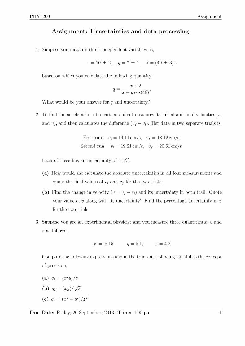
1. Suppose you measure three independent variables as,
x = 10 ± 2, y = 7 ± 1, θ = (40 ± 3).
based on which you calculate the following quantity,
q =x+ 2
x+ y cos(4θ),
What would be your answer for q and uncertainty?
2. To find the acceleration of a cart, a student measures its initial and final velocities, vi
and vf , and then calculates the difference (vf − vi). Her data in two separate trials is,
First run: vi = 14.11 cm/s, vf = 18.12 cm/s.
Second run: vi = 19.21 cm/s, vf = 20.61 cm/s.
Each of these has an uncertainty of ± 1%.
(a) How would she calculate the absolute uncertainties in all four measurements and
quote the final values of vi and vf for the two trials.
(b) Find the change in velocity (v = vf − vi) and its uncertainty in both trail. Quote
your value of v along with its uncertainty? Find the percentage uncertainty in v
for the two trials.
3. Suppose you are an experimental physicist and you measure three quantities x, y and
z as follows,
x = 8.15, y = 5.1, z = 4.2
Compute the following expressions and in the true spirit of being faithful to the concept
of precision,
(a) q1 = (x2y)/z
(b) q2 = (xy)/√z
(c) q3 = (x2 − y2)/z2
Due Date: Friday, 20 September, 2013. Time: 4:00 pm 1
PHY- 200 Assignment
8.16 8.14 8.12 8.16 8.18 8.10 8.18 8.18 8.18 8.24
8.16 8.14 8.17 8.18 8.21 8.12 8.12 8.17 8.06 8.10
8.12 8.10 8.14 8.09 8.16 8.16 8.21 8.14 8.16 8.13
TABLE I: Model data of time t (s).
4. (a) Calculate the mean and standard deviation for the following 30 measurements of
a time t (s),
(b) After several measurements, we can expect about 68% of the observed values to
be within σt of < t > (i.e., < t > ±σt).
(c) For the measurements of part (a),
How many would you expect to lie the range (< t > ±σt)? How many actually
do?
(d) How many would you expect to lie the range (< t > ± 2σt)? How many actually
do?
(e) What does 2σt correspond to?
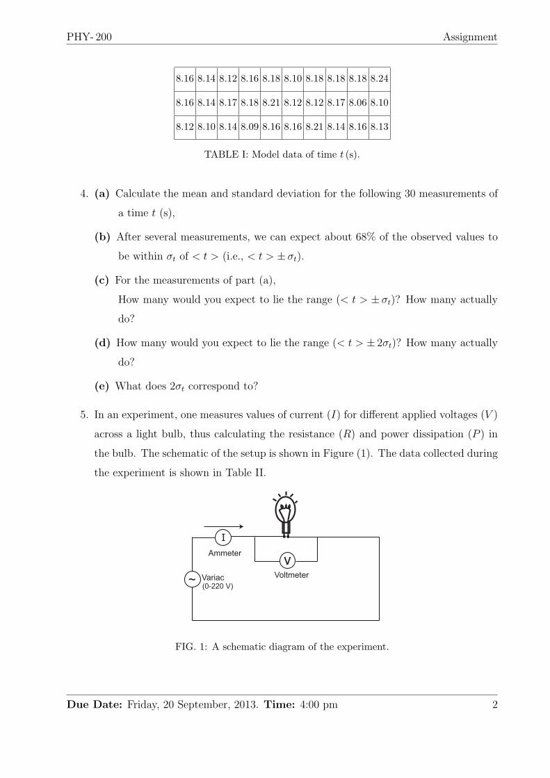
5. In an experiment, one measures values of current (I) for different applied voltages (V )
across a light bulb, thus calculating the resistance (R) and power dissipation (P ) in
the bulb. The schematic of the setup is shown in Figure (1). The data collected during
the experiment is shown in Table II.
V
I
Voltmeter
Ammeter
~ Variac (0-220 V)
FIG. 1: A schematic diagram of the experiment.
Due Date: Friday, 20 September, 2013. Time: 4:00 pm 2
PHY- 200 Assignment
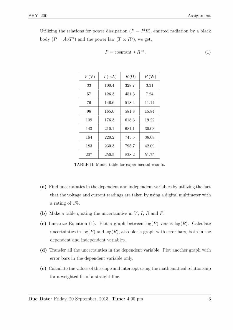
Utilizing the relations for power dissipation (P = I2R), emitted radiation by a black
body (P = AσT 4) and the power law (T ∝ Rγ), we get,
P = cosntant ∗R 4γ. (1)
V (V) I (mA) R (Ω) P (W)
33 100.4 328.7 3.31
57 126.3 451.3 7.24
76 146.6 518.4 11.14
96 165.0 581.8 15.84
109 176.3 618.3 19.22
143 210.1 681.1 30.03
164 220.2 745.5 36.08
183 230.3 795.7 42.09
207 250.5 828.2 51.75
TABLE II: Model table for experimental results.
(a) Find uncertainties in the dependent and independent variables by utilizing the fact
that the voltage and current readings are taken by using a digital multimeter with
a rating of 1%.
(b) Make a table quoting the uncertainties in V , I, R and P .
(c) Linearize Equation (1). Plot a graph between log(P ) versus log(R). Calculate
uncertainties in log(P ) and log(R), also plot a graph with error bars, both in the
dependent and independent variables.
(d) Transfer all the uncertainties in the dependent variable. Plot another graph with
error bars in the dependent variable only.
(e) Calculate the values of the slope and intercept using the mathematical relationship
for a weighted fit of a straight line.
Due Date: Friday, 20 September, 2013. Time: 4:00 pm 3
PHY- 200 Assignment
6. In an experiment to find the acceleration of gravity (g) using a simple pendulum,
a student records the following readings for the time period (T ) and length of the
pendulum (l),
Length, l (cm): 57.3 61.1 73.2 83.7 95.0
Time, T (s): 1.521 1.567 1.718 1.835 1.952
The length of the pendulum (l) is measured by a ruler, which is an analog device, and
a time is measured using a digital stopwatch (rating= 0).
The student uses the following relation to calculate (g),
g =4π2l
T 2. (2)
(a) Calculate the uncertainty in each reading of l and T using probability distribution
function and record them in a table.
(b) The relation for the time period is given as,
T = 2π
√l
g. (3)
Using Matlab, draw a plot between T and√l, also calculate slope of the straight
line using least squares curve fitting.
(c) Plot uncertainties in T and√l along with errobars.
Due Date: Friday, 20 September, 2013. Time: 4:00 pm 4
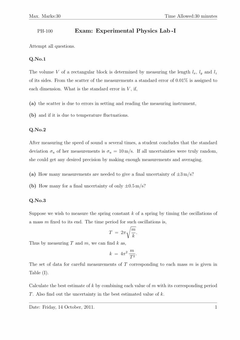
Max. Marks:30 Time Allowed:30 minutes
PH-100 Exam: Experimental Physics Lab -I
Attempt all questions.
Q.No.1
The volume V of a rectangular block is determined by measuring the length lx, ly and lz
of its sides. From the scatter of the measurements a standard error of 0.01% is assigned to
each dimension. What is the standard error in V , if,
(a) the scatter is due to errors in setting and reading the measuring instrument,
(b) and if it is due to temperature fluctuations.
Q.No.2
After measuring the speed of sound u several times, a student concludes that the standard
deviation σu of her measurements is σu = 10m/s. If all uncertainties were truly random,
she could get any desired precision by making enough measurements and averaging.
(a) How many measurements are needed to give a final uncertainty of ±3m/s?
(b) How many for a final uncertainty of only ±0.5m/s?
Q.No.3
Suppose we wish to measure the spring constant k of a spring by timing the oscillations of
a mass m fixed to its end. The time period for such oscillations is,
T = 2π
√m
k.
Thus by measuring T and m, we can find k as,
k = 4π2 m
T 2.
The set of data for careful measurements of T corresponding to each mass m is given in
Table (I).
Calculate the best estimate of k by combining each value of m with its corresponding period
T . Also find out the uncertainty in the best estimated value of k.
Date: Friday, 14 October, 2011. 1

Max. Marks:30 Time Allowed:30 minutes
Mass m (kg) 0.513 0.581 0.634 0.691 0.752 0.834 0.901 0.950
Period T (s) 1.24 1.33 1.36 1.44 1.50 1.59 1.65 1.69
TABLE I: Measured values of mass and time period.
Date: Friday, 14 October, 2011. 2
Solution key for the exam
Amrozia Shaheen and Muhammad Sabieh AnwarLUMS School of Science and Engineering
October 19, 2011
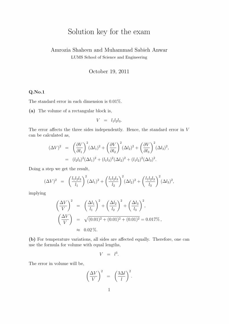
Q.No.1
The standard error in each dimension is 0.01%.
(a) The volume of a rectangular block is,
V = l1l2l3.
The error affects the three sides independently. Hence, the standard error in Vcan be calculated as,
(∆V )2 =
(∂V
∂l1
)2
(∆l1)2 +
(∂V
∂l2
)2
(∆l2)2 +
(∂V
∂l3
)2
(∆l3)2,
= (l2l3)2(∆l1)
2 + (l1l3)2(∆l2)
2 + (l1l2)2(∆l3)
2.
Doing a step we get the result,
(∆V )2 =
(l1l2l3l1
)2
(∆l1)2 +
(l1l2l3l2
)2
(∆l2)2 +
(l1l2l3l3
)2
(∆l3)2,
implying (∆V
V
)2
=
(∆l1l1
)2
+
(∆l2l2
)2
+
(∆l3l3
)2
,(∆V
V
)=
√(0.01)2 + (0.01)2 + (0.01)2 = 0.017% ,
≈ 0.02%.
(b) For temperature variations, all sides are affected equally. Therefore, one canuse the formula for volume with equal lengths,
V = l3.
The error in volume will be, (∆V
V
)2
=
(3∆l
l
)2
.
1
(∆V
V
)=
(3∆l
l
),
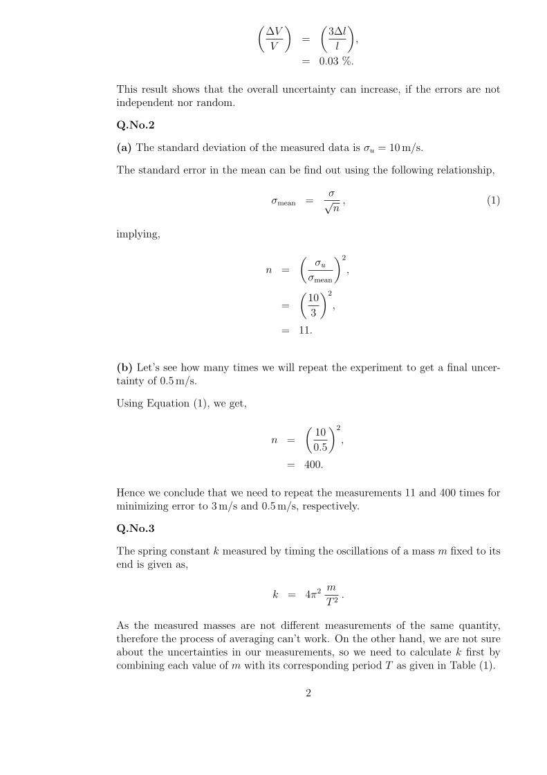
= 0.03 %.
This result shows that the overall uncertainty can increase, if the errors are notindependent nor random.
Q.No.2
(a) The standard deviation of the measured data is σu = 10m/s.
The standard error in the mean can be find out using the following relationship,
σmean =σ√n, (1)
implying,
n =
(σu
σmean
)2
,
=
(10
3
)2
,
= 11.
(b) Let’s see how many times we will repeat the experiment to get a final uncer-tainty of 0.5m/s.
Using Equation (1), we get,
n =
(10
0.5
)2
,
= 400.
Hence we conclude that we need to repeat the measurements 11 and 400 times forminimizing error to 3m/s and 0.5m/s, respectively.
Q.No.3
The spring constant k measured by timing the oscillations of a mass m fixed to itsend is given as,
k = 4π2 m
T 2.
As the measured masses are not different measurements of the same quantity,therefore the process of averaging can’t work. On the other hand, we are not sureabout the uncertainties in our measurements, so we need to calculate k first bycombining each value of m with its corresponding period T as given in Table (1).
2
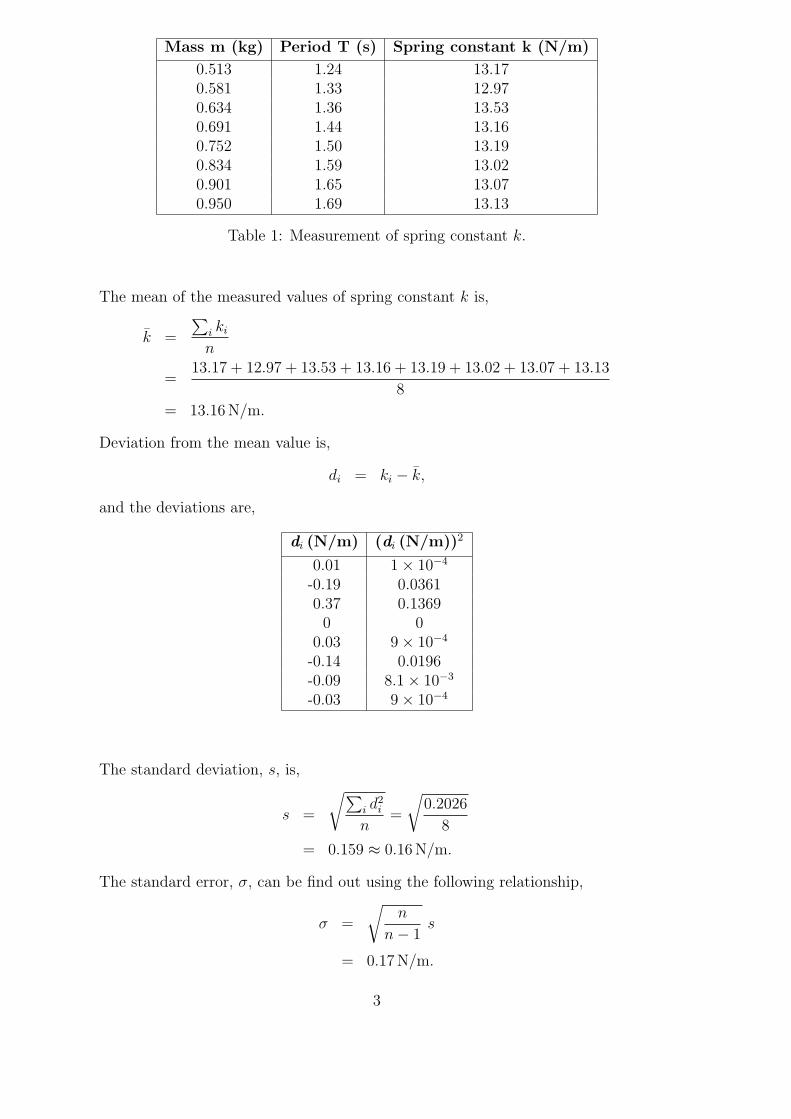
Mass m (kg) Period T (s) Spring constant k (N/m)
0.513 1.24 13.170.581 1.33 12.970.634 1.36 13.530.691 1.44 13.160.752 1.50 13.190.834 1.59 13.020.901 1.65 13.070.950 1.69 13.13
Table 1: Measurement of spring constant k.
The mean of the measured values of spring constant k is,
k =
∑i kin
=13.17 + 12.97 + 13.53 + 13.16 + 13.19 + 13.02 + 13.07 + 13.13
8
= 13.16N/m.
Deviation from the mean value is,
di = ki − k,
and the deviations are,
di (N/m) (di (N/m))2
0.01 1× 10⁻⁴
-0.19 0.03610.37 0.13690 0
0.03 9× 10⁻⁴
-0.14 0.0196-0.09 8.1× 10⁻³
-0.03 9× 10⁻⁴
The standard deviation, s, is,
s =
√∑i d
2i
n=
√0.2026
8
= 0.159 ≈ 0.16N/m.
The standard error, σ, can be find out using the following relationship,
σ =
√n
n− 1s
= 0.17N/m.
3
We can say that he expected standard error is approximately equal to the standarddeviation, σ ≈ s.
Now the standard error in the mean is,
σm =σ√n
= 0.06N/m.
Hence the final result can be written as,
k = (13.16± 0.06)N/m.
4
PHY- 200 Assignment (Solution)
Solution Assignment: Uncertainties and data
processing
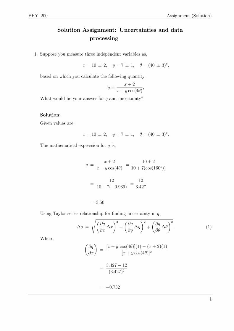
1. Suppose you measure three independent variables as,
x = 10 ± 2, y = 7 ± 1, θ = (40 ± 3).
based on which you calculate the following quantity,
q =x+ 2
x+ y cos(4θ),
What would be your answer for q and uncertainty?
Solution:
Given values are:
x = 10 ± 2, y = 7 ± 1, θ = (40 ± 3).
The mathematical expression for q is,
q =x+ 2
x+ y cos(4θ)=
10 + 2
10 + 7(cos(160))
=12
10 + 7(−0.939)=
12
3.427
= 3.50
Using Taylor series relationship for finding uncertainty in q,
∆q =
√(∂q
∂x∆x
)2
+
(∂q
∂y∆y
)2
+
(∂q
∂θ∆θ
)2
. (1)
Where, (∂q
∂x
)=
[x+ y cos(4θ)](1)− (x+ 2)(1)
[x+ y cos(4θ)]2
=3.427− 12
(3.427)2
= −0.732
1
PHY- 200 Assignment (Solution)
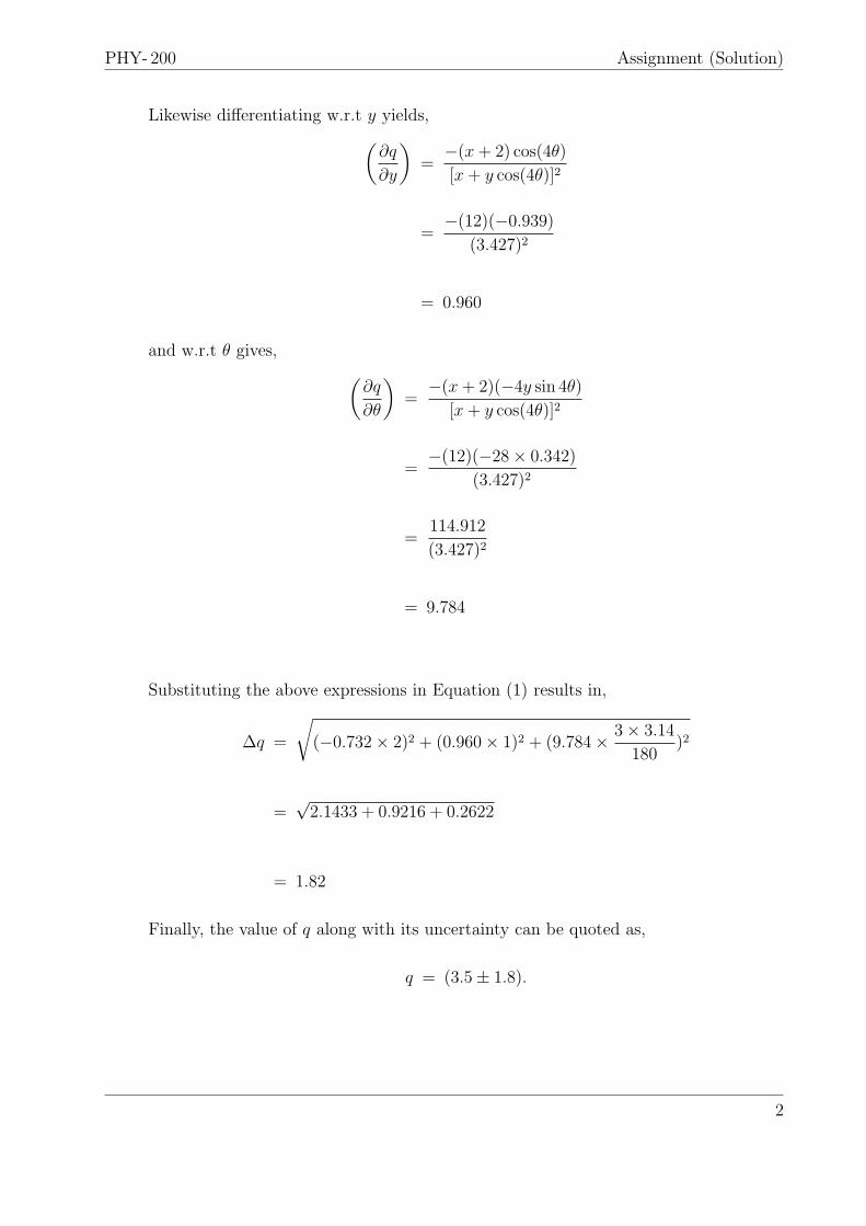
Likewise differentiating w.r.t y yields,(∂q
∂y
)=
−(x+ 2) cos(4θ)
[x+ y cos(4θ)]2
=−(12)(−0.939)
(3.427)2
= 0.960
and w.r.t θ gives, (∂q
∂θ
)=
−(x+ 2)(−4y sin 4θ)
[x+ y cos(4θ)]2
=−(12)(−28× 0.342)
(3.427)2
=114.912
(3.427)2
= 9.784
Substituting the above expressions in Equation (1) results in,
∆q =
√(−0.732× 2)2 + (0.960× 1)2 + (9.784× 3× 3.14
180)2
=√2.1433 + 0.9216 + 0.2622
= 1.82
Finally, the value of q along with its uncertainty can be quoted as,
q = (3.5± 1.8).
2
PHY- 200 Assignment (Solution)
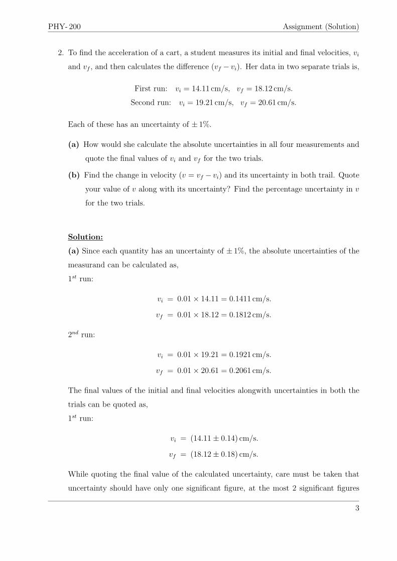
2. To find the acceleration of a cart, a student measures its initial and final velocities, vi
and vf , and then calculates the difference (vf − vi). Her data in two separate trials is,
First run: vi = 14.11 cm/s, vf = 18.12 cm/s.
Second run: vi = 19.21 cm/s, vf = 20.61 cm/s.
Each of these has an uncertainty of ± 1%.
(a) How would she calculate the absolute uncertainties in all four measurements and
quote the final values of vi and vf for the two trials.
(b) Find the change in velocity (v = vf − vi) and its uncertainty in both trail. Quote
your value of v along with its uncertainty? Find the percentage uncertainty in v
for the two trials.
Solution:
(a) Since each quantity has an uncertainty of ± 1%, the absolute uncertainties of the
measurand can be calculated as,
1st run:
vi = 0.01× 14.11 = 0.1411 cm/s.
vf = 0.01× 18.12 = 0.1812 cm/s.
2nd run:
vi = 0.01× 19.21 = 0.1921 cm/s.
vf = 0.01× 20.61 = 0.2061 cm/s.
The final values of the initial and final velocities alongwith uncertainties in both the
trials can be quoted as,
1st run:
vi = (14.11± 0.14) cm/s.
vf = (18.12± 0.18) cm/s.
While quoting the final value of the calculated uncertainty, care must be taken that
uncertainty should have only one significant figure, at the most 2 significant figures
3
PHY- 200 Assignment (Solution)
can be considered. After deciding about the significant figure, the best approximated
value can be rounded off so that the decimal places of the best estimated value and
uncertainty should be at the same position.
2nd run:
vi = (19.21± 0.19) cm/s.
vf = (20.61± 0.21) cm/s.
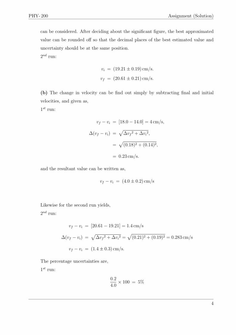
(b) The change in velocity can be find out simply by subtracting final and initial
velocities, and given as,
1st run:
vf − vi = [18.0− 14.0] = 4 cm/s,
∆(vf − vi) =√∆vf 2 +∆vi2,
=√(0.18)2 + (0.14)2,
= 0.23 cm/s.
and the resultant value can be written as,
vf − vi = (4.0± 0.2) cm/s
Likewise for the second run yields,
2nd run:
vf − vi = [20.61− 19.21] = 1.4 cm/s
∆(vf − vi) =√∆vf 2 +∆vi2 =
√(0.21)2 + (0.19)2 = 0.283 cm/s
vf − vi = (1.4± 0.3) cm/s.
The percentage uncertainties are,
1st run:
0.2
4.0× 100 = 5%
4
PHY- 200 Assignment (Solution)
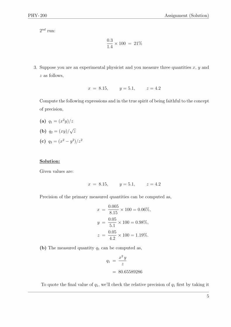
2nd run:
0.3
1.4× 100 = 21%
3. Suppose you are an experimental physicist and you measure three quantities x, y and
z as follows,
x = 8.15, y = 5.1, z = 4.2
Compute the following expressions and in the true spirit of being faithful to the concept
of precision,
(a) q1 = (x2y)/z
(b) q2 = (xy)/√z
(c) q3 = (x2 − y2)/z2
Solution:
Given values are:
x = 8.15, y = 5.1, z = 4.2
Precision of the primary measured quantities can be computed as,
x =0.005
8.15× 100 = 0.06%,
y =0.05
5.1× 100 = 0.98%,
z =0.05
4.2× 100 = 1.19%.
(b) The measured quantity q1 can be computed as,
q1 =x2 y
z
= 80.65589286
To quote the final value of q1, we’ll check the relative precision of q1 first by taking it
5
PHY- 200 Assignment (Solution)
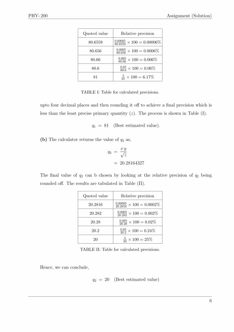
Quoted value Relative precision
80.6559 0.0000580.6559 × 100 = 0.00006%
80.656 0.000580.656 × 100 = 0.0006%
80.66 0.00580.66 × 100 = 0.006%
80.6 0.0580.6 × 100 = 0.06%
81 581 × 100 = 6.17%
TABLE I: Table for calculated precisions.
upto four decimal places and then rounding it off to achieve a final precision which is
less than the least precise primary quantity (z). The process is shown in Table (I).
q1 = 81 (Best estimated value).
(b) The calculator returns the value of q2 as,
q2 =x y√z
= 20.28164327
The final value of q2 can b chosen by looking at the relative precision of q2 being
rounded off. The results are tabulated in Table (II).
Quoted value Relative precision
20.2816 0.0000520.2816 × 100 = 0.0002%
20.282 0.000520.282 × 100 = 0.002%
20.28 0.00520.28 × 100 = 0.02%
20.2 0.0520.2 × 100 = 0.24%
20 520 × 100 = 25%
TABLE II: Table for calculated precisions.
Hence, we can conclude,
q2 = 20 (Best estimated value)
6
PHY- 200 Assignment (Solution)
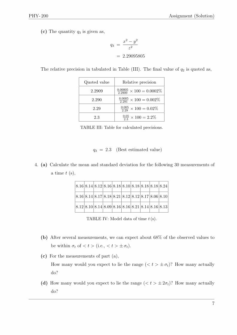
(c) The quantity q3 is given as,
q3 =x2 − y2
z2
= 2.29095805
The relative precision in tabulated in Table (III). The final value of q2 is quoted as,
Quoted value Relative precision
2.2909 0.000052.2909 × 100 = 0.0002%
2.290 0.00052.291 × 100 = 0.002%
2.29 0.0052.29 × 100 = 0.02%
2.3 0.052.3 × 100 = 2.2%
TABLE III: Table for calculated precisions.
q3 = 2.3 (Best estimated value)
4. (a) Calculate the mean and standard deviation for the following 30 measurements of
a time t (s),
8.16 8.14 8.12 8.16 8.18 8.10 8.18 8.18 8.18 8.24
8.16 8.14 8.17 8.18 8.21 8.12 8.12 8.17 8.06 8.10
8.12 8.10 8.14 8.09 8.16 8.16 8.21 8.14 8.16 8.13
TABLE IV: Model data of time t (s).
(b) After several measurements, we can expect about 68% of the observed values to
be within σt of < t > (i.e., < t > ±σt).
(c) For the measurements of part (a),
How many would you expect to lie the range (< t > ±σt)? How many actually
do?
(d) How many would you expect to lie the range (< t > ± 2σt)? How many actually
do?
7
PHY- 200 Assignment (Solution)
(e) What does 2σt correspond to?
Solution:
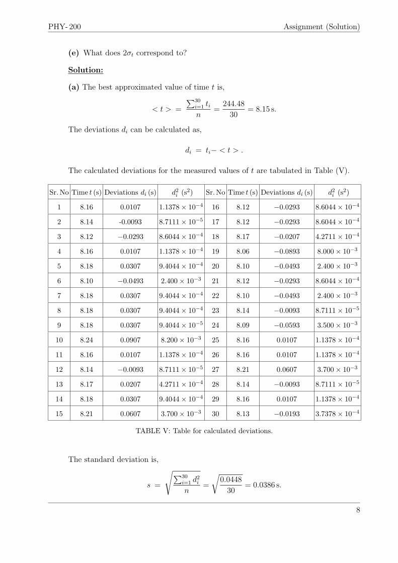
(a) The best approximated value of time t is,
< t > =
∑30i=1 tin
=244.48
30= 8.15 s.
The deviations di can be calculated as,
di = ti− < t > .
The calculated deviations for the measured values of t are tabulated in Table (V).
Sr.No Time t (s) Deviations di (s) d2i (s2) Sr. No Time t (s) Deviations di (s) d2i (s2)
1 8.16 0.0107 1.1378× 10⁻⁴ 16 8.12 −0.0293 8.6044× 10⁻⁴
2 8.14 -0.0093 8.7111× 10⁻⁵ 17 8.12 −0.0293 8.6044× 10⁻⁴
3 8.12 −0.0293 8.6044× 10⁻⁴ 18 8.17 −0.0207 4.2711× 10⁻⁴
4 8.16 0.0107 1.1378× 10⁻⁴ 19 8.06 −0.0893 8.000× 10⁻³
5 8.18 0.0307 9.4044× 10⁻⁴ 20 8.10 −0.0493 2.400× 10⁻³
6 8.10 −0.0493 2.400× 10⁻³ 21 8.12 −0.0293 8.6044× 10⁻⁴
7 8.18 0.0307 9.4044× 10⁻⁴ 22 8.10 −0.0493 2.400× 10⁻³
8 8.18 0.0307 9.4044× 10⁻⁴ 23 8.14 −0.0093 8.7111× 10⁻⁵
9 8.18 0.0307 9.4044× 10⁻⁵ 24 8.09 −0.0593 3.500× 10⁻³
10 8.24 0.0907 8.200× 10⁻³ 25 8.16 0.0107 1.1378× 10⁻⁴
11 8.16 0.0107 1.1378× 10⁻⁴ 26 8.16 0.0107 1.1378× 10⁻⁴
12 8.14 −0.0093 8.7111× 10⁻⁵ 27 8.21 0.0607 3.700× 10⁻³
13 8.17 0.0207 4.2711× 10⁻⁴ 28 8.14 −0.0093 8.7111× 10⁻⁵
14 8.18 0.0307 9.4044× 10⁻⁴ 29 8.16 0.0107 1.1378× 10⁻⁴
15 8.21 0.0607 3.700× 10⁻³ 30 8.13 −0.0193 3.7378× 10⁻⁴
TABLE V: Table for calculated deviations.
The standard deviation is,
s =
√∑30i=1 d
2i
n=
√0.0448
30= 0.0386 s.
8
PHY- 200 Assignment (Solution)
The standard uncertainty can be calculated as,
σ =
√n
n− 1(s) =
√30
29(0.0386) = 0.0393 = 0.04 s,
and standard uncertainty in the mean value is,
σm =σ√n=
0.0393√30
= 0.0072, s
= 0.01 s.
The best estimated value of time t can be quoted as,
t = (8.15± 0.01) s
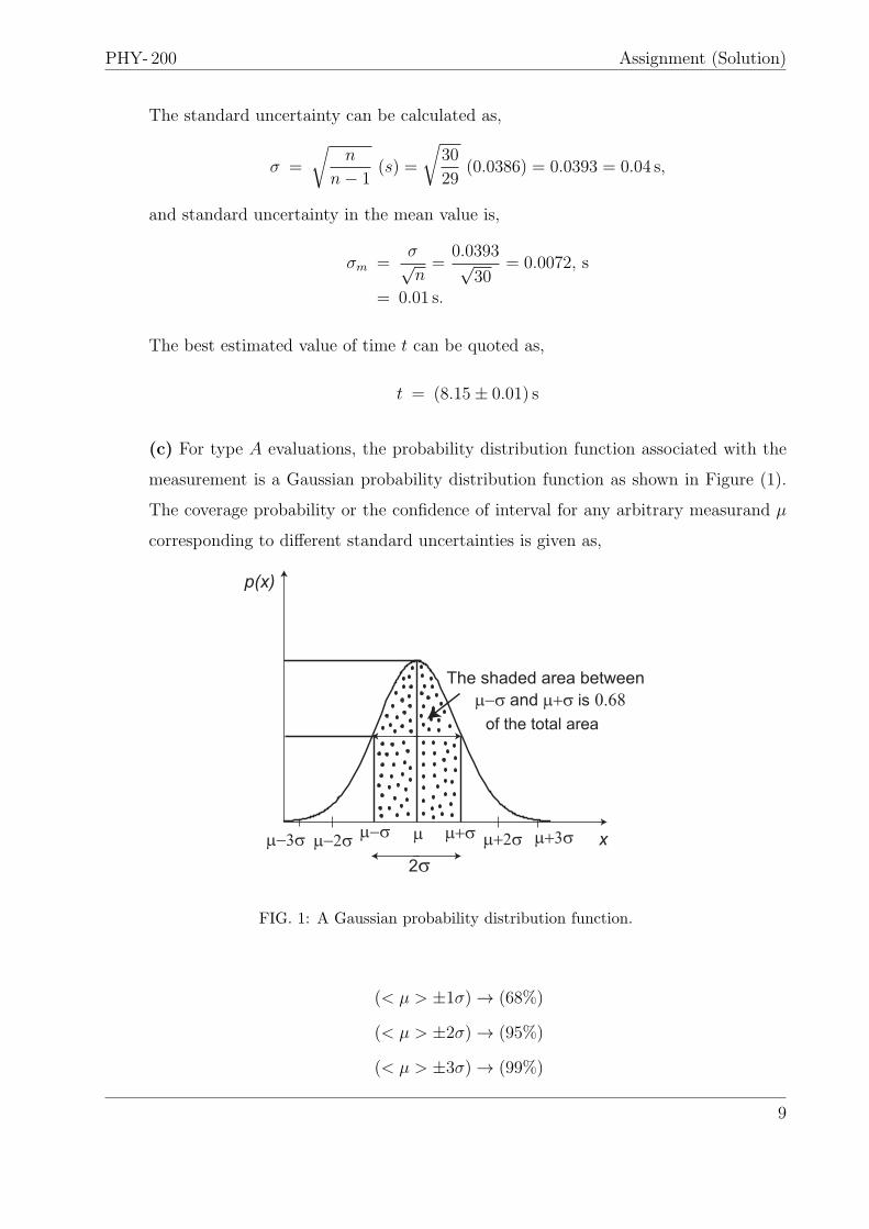
(c) For type A evaluations, the probability distribution function associated with the
measurement is a Gaussian probability distribution function as shown in Figure (1).
The coverage probability or the confidence of interval for any arbitrary measurand µ
corresponding to different standard uncertainties is given as,
µ µ+σµ−σ
2σ
The shaded area between
µ−σ and µ+σ is 0.68
p(x)
x
of the total area
µ+2σ µ+3σµ−2σµ−3σ
FIG. 1: A Gaussian probability distribution function.
(< µ > ±1σ) → (68%)
(< µ > ±2σ) → (95%)
(< µ > ±3σ) → (99%)
9
PHY- 200 Assignment (Solution)
Now as the above expressions predict, the 68% confidence of interval corresponds to
(< t > ±1σ). Considering this, the range of interval becomes,
t = (8.15± 0.04) s
t = [8.11, 8.19] s.
The values (in seconds s) that lie within 68% confidence of interval are,
8.16, 8.14, 8.12, 8.16, 8.18, 8.10, 8.18, 8.18, 8.18, 8.16, 8.14, 8.17, 8.18,
8.12, 8.12, 8.17, 8.10, 8.12, 8.10, 8.14, 8.16, 8.16, 8.14, 8.16, 8.13.
and values (in seconds s) which lie outside this interval or lying within 32% confidence
of interval are,
8.24, 8.21, 8.06, 8.09, 8.21.
(d) The 95% confidence of interval corresponds to (< t > ±2σ). The range of interval
becomes,
t = (8.15± 2(0.04)) s = (8.15± 0.08) s,
t = [8.07, 8.23] s.
The values (in seconds s) that lie within 95% confidence of interval are,
8.16, 8.14, 8.12, 8.16, 8.18, 8.10, 8.18, 8.18, 8.18, 8.16, 8.14, 8.17, 8.18, 8.12,
8.12, 8.17, 8.10, 8.12, 8.10, 8.14, 8.16, 8.16, 8.14, 8.16, 8.13, 8.09, 8.21, 8.21.
and values (in seconds s) which lie outside this interval or lying within 5% confidence
of interval are,
8.06, 8.24.
(e) 2σt corresponds to the 95% confidence of interval. This means that there is 95%
probability that the best approximated value of measurand lies somewhere within the
interval (< t > ±2σ) of standard uncertainty. Conversely, there is 5% probability that
the best approximated value of the measurand lies outside the interval (< t > ±2σ).
10
PHY- 200 Assignment (Solution)
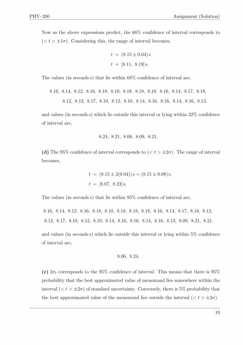
5. In an experiment, one measures values of current (I) for different applied voltages (V )
across a light bulb, thus calculating the resistance (R) and power dissipation (P ) in
the bulb. The schematic of the setup is shown in Figure (2). The data collected during
the experiment is shown in Table X.
V
I
Voltmeter
Ammeter
~ Variac (0-220 V)
FIG. 2: A schematic diagram of the experiment.
Utilizing the relations for power dissipation (P = I2R), emitted radiation by a black
body (P = AσT 4) and the power law (T ∝ Rγ), we get,
P = cosntant ∗R 4γ. (2)
(a) Find uncertainties in the dependent and independent variables by utilizing the fact
that the voltage and current readings are taken by using a digital multimeter with
a rating of 1%.
(b) Make a table quoting the uncertainties in V , I, R and P .
(c) Linearize Equation (2). Plot a graph between log(P ) versus log(R). Calculate
uncertainties in log(P ) and log(R), also plot a graph with error bars, both in the
dependent and independent variables.
(d) Transfer all the uncertainties in the dependent variable. Plot another graph with
error bars in the dependent variable only.
(e) Calculate the values of the slope and intercept using the mathematical relationship
for a weighted fit of a straight line.
11
PHY- 200 Assignment (Solution)
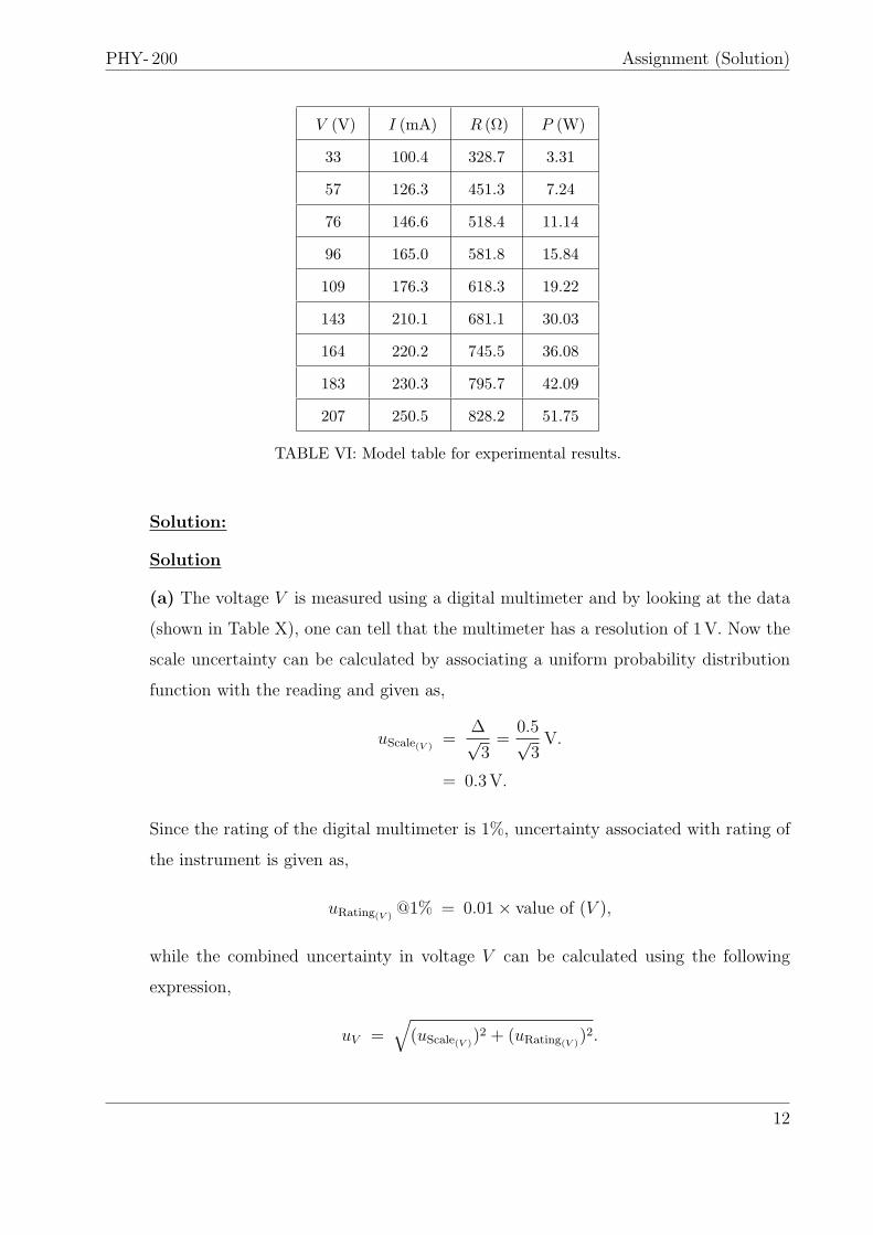
V (V) I (mA) R (Ω) P (W)
33 100.4 328.7 3.31
57 126.3 451.3 7.24
76 146.6 518.4 11.14
96 165.0 581.8 15.84
109 176.3 618.3 19.22
143 210.1 681.1 30.03
164 220.2 745.5 36.08
183 230.3 795.7 42.09
207 250.5 828.2 51.75
TABLE VI: Model table for experimental results.
Solution:
Solution
(a) The voltage V is measured using a digital multimeter and by looking at the data
(shown in Table X), one can tell that the multimeter has a resolution of 1V. Now the
scale uncertainty can be calculated by associating a uniform probability distribution
function with the reading and given as,
uScale(V )=
∆√3=
0.5√3V.
= 0.3V.
Since the rating of the digital multimeter is 1%, uncertainty associated with rating of
the instrument is given as,
uRating(V )@1% = 0.01× value of (V ),
while the combined uncertainty in voltage V can be calculated using the following
expression,
uV =√(uScale(V )
)2 + (uRating(V ))2.
12
PHY- 200 Assignment (Solution)
Likewise for the ammeter, the scale and combine uncertainty can be calculated as,
uScaleI =∆√3=
0.05√3mA = 0.03× 10⁻³A.
uI =√
(uScale(I))2 + (uRating(I))
2.
The uncertainty in energy (R = V/I) can be calculated using Taylor series approxi-
mation,
∆R =
√(∂R
∂V∆V
)2
+
(∂R
∂I∆I
)2
, (3)
By looking at Equation (4), we can easily tell that the dependent variable is log(P ),
while the independent one is log(R). Now the question is how to propagate uncertain-
ties from P and R to log(P ) and log(R), respectively. For that we’ll utilize the general
rule of propagation,
ux = ∆(logR) =
√(∂(logR)
∂R∆R
)2
=∆R
R,
uy = ∆(logP ) =
√(∂(logP )
∂P∆P
)2
=∆P
P.
(b) Uncertainties in all the measured and inferred quantities are quoted in Table (VII).
(c) By taking log on both sides of Equation (2) yields a straight line equation given
as,
log(P ) = 4γ log(R) + log(c), (4)
where (logP ) is the dependent variable, (logR) is the independent variable,
(c=constant) and the value of γ can be calculated by finding the value of slope.
Graph is shown in Figure (3a).
(d)The mathematical expressions for transferring uncertainties to the dependent vari-
able (logP ) and for calculating the total uncertainty are,
uTrans =
(dy
dx
)ux = (3)ux, (5)
uTotal =√(uTrans)2 + u2
y. (6)
13
PHY- 200 Assignment (Solution)
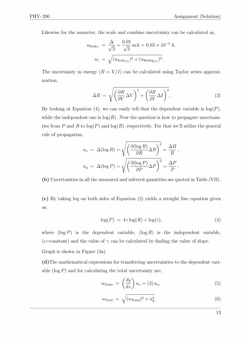
Voltage ∆V Current I ∆I Resistance ∆R Power dissip- ∆P log(R) ∆(logR) log(P ) ∆(logP )
V (V) (V) ×10−3 (A) ×10−3(A) R (Ω) (Ω) ationP (W) (W)
33.0 0.4 100.4 1.0 328.7 5.5 3.3 0.1 5.79 0.02 1.19 0.03
57.0 0.6 126.3 1.3 451.3 6.8 7.2 0.2 6.11 0.02 1.97 0.03
76.0 0.8 146.6 1.5 518.4 7.6 11.1 0.3 6.25 0.01 2.41 0.02
96 1 165.0 1.7 581.8 8.4 15.8 0.4 6.37 0.01 2.76 0.02
109.0 1.1 176.3 1.8 618.3 8.9 19.2 0.5 6.43 0.01 2.95 0.02
143.0 1.4 210.0 2.1 681.0 9.7 30.0 0.7 6.52 0.01 3.40 0.02
164.0 1.7 220.0 2.2 745.5 10.6 36.1 0.9 6.61 0.01 3.59 0.02
183.0 1.9 230.0 2.3 795.7 11.3 42.0 1.0 6.68 0.01 3.74 0.02
207 2. 250.0 2.5 828.0 11.8 51.8 1.3 6.72 0.01 3.95 0.02
TABLE VII: Experimental data and calculated uncertainties.
The weights w are reciprocal squares of the total uncertainty being utilized in least-
squares fitting of a straight line. The expression for calculating the weight w is,
w =1
u2Total
. (7)
The uncertainties calculated for the given data of independent (logR) and dependent
variables (logP ) are shown in Table (VIII).
Graph with error bars only in the dependent variable is shown in Figure (3b).
(e) The mathematical relationships for slope (m) and intercept (c) are,
m =Σiwi Σiwi(xiyi)− Σi(wixi) Σi(wiyi)
Σiwi Σi(wx2i )− (Σiwixi)2
, (8)
and,
c =Σi(wix
2i ) Σi(wiyi)− Σi(wixi) Σi(wixiyi)
ΣiwiΣi(wix2i )− (Σiwixi)2
, (9)
where x is the independent variable (logR in our case), y is the dependent variable
(logP ) and w is the weight.
The different terms in the numerator and denominator of Equations (8) and (9) are
calculated separately and tabulated in Table (IX).
14
PHY- 200 Assignment (Solution)
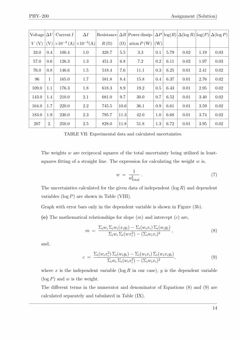
log(R) log(P ) uTrans uTotal
5.79 1.19 0.050 0.057
6.11 1.97 0.045 0.052
6.25 2.41 0.044 0.051
6.37 2.76 0.044 0.050
6.43 2.95 0.043 0.050
6.52 3.40 0.043 0.049
6.61 3.59 0.043 0.049
6.68 3.74 0.043 0.049
6.72 3.95 0.0423 0.049
TABLE VIII: Calculated data for the transfer and total uncertainties.
w wxy wx wy wx2
309.8185 0.2149× 10⁴ 1.7954× 10³ 0.3708× 10³ 1.0405× 10⁴
373.4411 0.4506× 10⁴ 2.2825× 10³ 0.7372× 10³ 1.3951× 10⁴
391.1746 0.5894× 10⁴ 2.4451× 10³ 0.9429× 10³ 1.5284× 10⁴
400.3012 0.7040× 10⁴ 2.5484× 10³ 1.1058× 10³ 1.6223× 10⁴
403.8517 0.7672× 10⁴ 2.5955× 10³ 1.1938× 10³ 1.6681× 10⁴
409.1155 0.9080× 10⁴ 2.6689× 10³ 1.3919× 10³ 1.7411× 10⁴
410.8932 0.9745× 10⁴ 2.7177× 10³ 1.4734× 10³ 1.7975× 10⁴
412.0122 1.0292× 10⁴ 2.7519× 10³ 1.5408× 10³ 1.8381× 10⁴
413.0174 1.0952× 10⁴ 2.7751× 10³ 1.6299× 10³ 1.8646× 10⁴∑w = 3523.6
∑wxy = 67330
∑wx = 22581
∑wy = 10387
∑wx2 = 144960
TABLE IX: Terms being utilized in finding the values of slope and intercept.
Substituting the calculated terms given in Table (IX) in Equation (8) yields,
m =(3523.6)(67330)− (22581)(10387)
(3523.6)(144960)− (22581)2,
= 3.041
15
PHY- 200 Assignment (Solution)
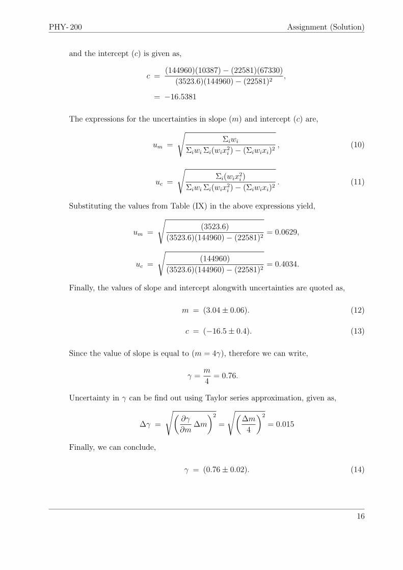
and the intercept (c) is given as,
c =(144960)(10387)− (22581)(67330)
(3523.6)(144960)− (22581)2,
= −16.5381
The expressions for the uncertainties in slope (m) and intercept (c) are,
um =
√Σiwi
ΣiwiΣi(wix2i )− (Σiwixi)2
, (10)
uc =
√Σi(wix2
i )
ΣiwiΣi(wix2i )− (Σiwixi)2
. (11)
Substituting the values from Table (IX) in the above expressions yield,
um =
√(3523.6)
(3523.6)(144960)− (22581)2= 0.0629,
uc =
√(144960)
(3523.6)(144960)− (22581)2= 0.4034.
Finally, the values of slope and intercept alongwith uncertainties are quoted as,
m = (3.04± 0.06). (12)
c = (−16.5± 0.4). (13)
Since the value of slope is equal to (m = 4γ), therefore we can write,
γ =m
4= 0.76.
Uncertainty in γ can be find out using Taylor series approximation, given as,
∆γ =
√(∂γ
∂m∆m
)2
=
√(∆m
4
)2
= 0.015
Finally, we can conclude,
γ = (0.76± 0.02). (14)
16
PHY- 200 Assignment (Solution)
5.6 5. 8 6.0 6.2 6.4 6.6 6.8 7.01.0
1.5
2.0
2.5
3.0
3.5
4.0
log(R)
log(P)
1.0
1.5
2.0
2.5
3.0
3.5
4.0
log(P)
5.6 5. 8 6.0 6.2 6.4 6.6 6.8 7.0
log(R)
(a) (b)
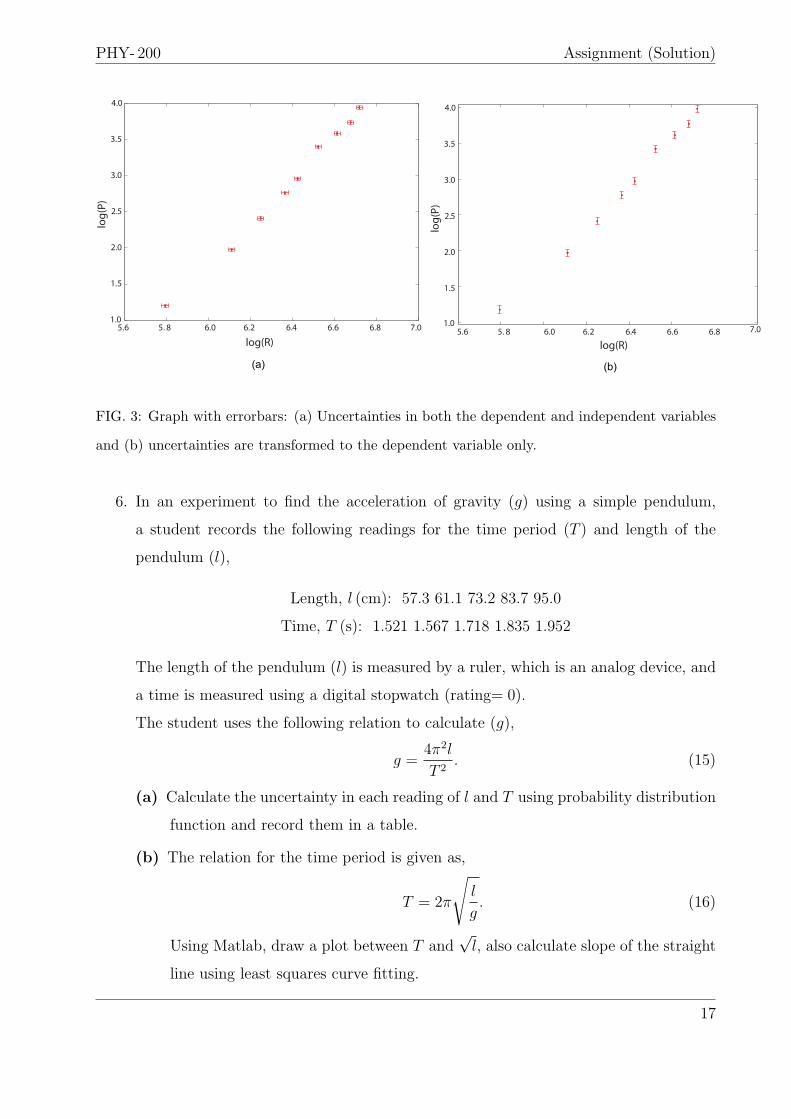
FIG. 3: Graph with errorbars: (a) Uncertainties in both the dependent and independent variables
and (b) uncertainties are transformed to the dependent variable only.
6. In an experiment to find the acceleration of gravity (g) using a simple pendulum,
a student records the following readings for the time period (T ) and length of the
pendulum (l),
Length, l (cm): 57.3 61.1 73.2 83.7 95.0
Time, T (s): 1.521 1.567 1.718 1.835 1.952
The length of the pendulum (l) is measured by a ruler, which is an analog device, and
a time is measured using a digital stopwatch (rating= 0).
The student uses the following relation to calculate (g),
g =4π2l
T 2. (15)
(a) Calculate the uncertainty in each reading of l and T using probability distribution
function and record them in a table.
(b) The relation for the time period is given as,
T = 2π
√l
g. (16)
Using Matlab, draw a plot between T and√l, also calculate slope of the straight
line using least squares curve fitting.
17
PHY- 200 Assignment (Solution)
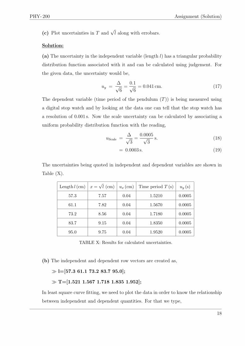
(c) Plot uncertainties in T and√l along with errobars.
Solution:
(a) The uncertainty in the independent variable (length l) has a triangular probability
distribution function associated with it and can be calculated using judgement. For
the given data, the uncertainty would be,
uy =∆√6=
0.1√6= 0.041 cm. (17)
The dependent variable (time period of the pendulum (T )) is being measured using
a digital stop watch and by looking at the data one can tell that the stop watch has
a resolution of 0.001 s. Now the scale uncertainty can be calculated by associating a
uniform probability distribution function with the reading,
uScale =∆√3=
0.0005√3
s. (18)
= 0.0003 s. (19)
The uncertainties being quoted in independent and dependent variables are shown in
Table (X).
Length l (cm) x =√l (cm) ux (cm) Time period T (s) uy (s)
57.3 7.57 0.04 1.5210 0.0005
61.1 7.82 0.04 1.5670 0.0005
73.2 8.56 0.04 1.7180 0.0005
83.7 9.15 0.04 1.8350 0.0005
95.0 9.75 0.04 1.9520 0.0005
TABLE X: Results for calculated uncertainties.
(b) The independent and dependent row vectors are created as,
≫ l=[57.3 61.1 73.2 83.7 95.0];
≫ T=[1.521 1.567 1.718 1.835 1.952];
In least square curve fitting, we need to plot the data in order to know the relationship
between independent and dependent quantities. For that we type,
18
PHY- 200 Assignment (Solution)
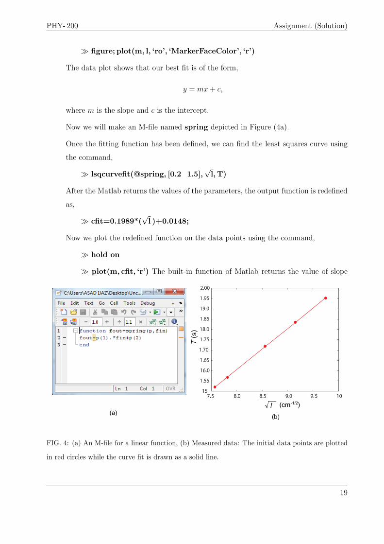
≫ figure; plot(m, l, ‘ro’, ‘MarkerFaceColor’, ‘r’)
The data plot shows that our best fit is of the form,
y = mx+ c,
where m is the slope and c is the intercept.
Now we will make an M-file named spring depicted in Figure (4a).
Once the fitting function has been defined, we can find the least squares curve using
the command,
≫ lsqcurvefit(@spring, [0.2 1.5],√l, T)
After the Matlab returns the values of the parameters, the output function is redefined
as,
≫ cfit=0.1989*(√l )+0.0148;
Now we plot the redefined function on the data points using the command,
≫ hold on
≫ plot(m, cfit, ‘r’) The built-in function of Matlab returns the value of slope
7.5 8.0 8.5 9.0 9.5 101.5
1.55
1.6.0
1.65
1.70
1.75
1.8.0
1.85
1.9.0
1.95
2.00
T (
s)
1l (cm )-1/2
(a)(b)
FIG. 4: (a) An M-file for a linear function, (b) Measured data: The initial data points are plotted
in red circles while the curve fit is drawn as a solid line.
19
PHY- 200 Assignment (Solution)
and intercept. Utilizing the first value yield,
slope (m) = 0.1989 s cm−1/2 = (0.1989× 10) sm−1/2,
= 1.989 sm−1/2 = 2 sm−1/2. (20)
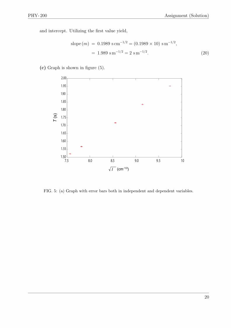
(c) Graph is shown in figure (5).
7.5 8.0 8.5 9.0 9.5 101.50
1.55
1.60
1.65
1.70
1.75
1.80
1.85
1.90
1.95
2.00
1l (cm )-1/2
T (
s)
FIG. 5: (a) Graph with error bars both in independent and dependent variables.
20
PHY-200 Quiz 1(1)
Quiz 1(1): Experimental Physics Lab-I
Solution
1. Suppose you measure three independent variables as,
x = 20.2 ± 1.5, y = 8.5 ± 0.5, θ = (30 ± 2).
Compute the following quantity,
q = x(y − sin θ).
Find the uncertainty in q and quote your results?
Solution:
Given values are:
x = 20.2 ± 1.5, y = 8.5 ± 0.5, θ = (30 ± 2).
Using the values given above, q becomes,
q = x(y − sin θ) = 20.2(8.5− sin 30),
= 20.2(8.5− 0.5) = 161.6
The uncertainty to the inferred quantity q can be find out using the following rela-
tionship,
∆q =
√(∂q
∂x∆x
)2
+
(∂q
∂y∆y
)2
+
(∂q
∂θ∆θ
)2
. (1)
The first expression on the R.H.S of Equation (1) can be obtained by differentiating q
w.r.t x and multiplying with ∆x,(∂q
∂x
)∆x = (y − sin θ)∆x = (8.5− sin 30)(1.5),
= (8.5− 0.5)1.5 = 12
Likewise differentiating w.r.t y yields,(∂q
∂y
)∆y = x∆y = (20.2)(0.5) = 10.1
September, 9, 2013 1
PHY-200 Quiz 1(1)
and w.r.t θ gives,(∂q
∂θ
)∆θ = (−x cos θ)∆θ = (−20.2× 0.866)
(2π
180
),
= 0.6103
Substituting the above expressions in Equation (1) results in,
q =√
(12)2 + (10.1)2 + (0.6103)2 ,
= 15.69
Finally, the value of q alongwith its uncertainty can be quoted as,
q = (162± 16).
2. A group of students measures g, the acceleration due to gravity, with a compound
pendulum and obtain the following values in units of ms−2.
9.81, 9.79, 9.84, 9.81, 9.75, 9.79, 9.82
(a) Calculate the mean and the standard deviation. Find the standard uncertainty
and quote your results.
(b) How many measurements would you expect to lie outside the 95% confidence
interval? How many actually do?
Solution:
(a) The best approximated value of acceleration due to gravity g is,
< g > =
∑7i=1 gin
=68.61
7= 9.80m/s2. (2)
The deviations di can be calculated as,
di = gi− < g > .
The calculated deviations for the measured values of g are tabulated in Table (I).
September, 9, 2013 2
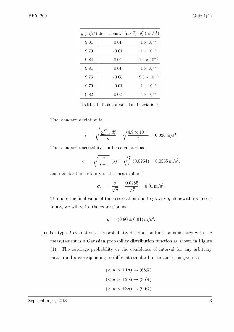
PHY-200 Quiz 1(1)
g (m/s2) deviations di (m/s2) d2i (m2/s4)
9.81 0.01 1× 10⁻⁴
9.79 -0.01 1× 10⁻⁴
9.84 0.04 1.6× 10⁻³
9.81 0.01 1× 10⁻⁴
9.75 -0.05 2.5× 10⁻³
9.79 -0.01 1× 10⁻⁴
9.82 0.02 4× 10⁻⁴
TABLE I: Table for calculated deviations.
The standard deviation is,
s =
√∑7i=1 d
2i
n=
√4.9× 10⁻³
7= 0.026m/s2.
The standard uncertainty can be calculated as,
σ =
√n
n− 1(s) =
√7
6(0.0264) = 0.0285m/s2,
and standard uncertainty in the mean value is,
σm =σ√n=
0.0285√7
= 0.01m/s2.
To quote the final value of the acceleration due to gravity g alongwith its uncer-
tainty, we will write the expression as,
g = (9.80± 0.01)m/s2.
(b) For type A evaluations, the probability distribution function associated with the
measurement is a Gaussian probability distribution function as shown in Figure
(1). The coverage probability or the confidence of interval for any arbitrary
measurand µ corresponding to different standard uncertainties is given as,
(< µ > ±1σ) → (68%)
(< µ > ±2σ) → (95%)
(< µ > ±3σ) → (99%)
September, 9, 2013 3
PHY-200 Quiz 1(1)
µ µ+σµ−σ
2σ
The shaded area between
µ−σ and µ+σ is 0.68
p(x)
x
of the total area
µ+2σ µ+3σµ−2σµ−3σ
FIG. 1: A Gaussian probability distribution function.
Now as the above expressions predict, the 95% confidence of interval corresponds
to (< g > ±2σ). Considering this, the range of interval becomes,
g = (9.80± 2(0.01))m/s2 = (9.80± 0.02)m/s2,
g = [9.78, 9.82]m/s2.
The values (in m/s2) that lie within 95% confidence of interval are,
9.79, 9.81, 9.81, 9.79, 9.82,
and values (in m/s2) which lie outside this interval or lying within 5% confidence
of interval are,
9.84, 9.75.
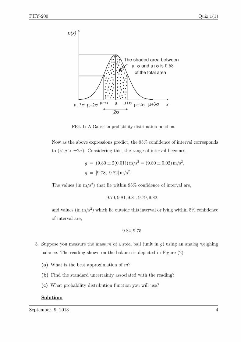
3. Suppose you measure the mass m of a steel ball (unit in g) using an analog weighing
balance. The reading shown on the balance is depicted in Figure (2).
(a) What is the best approximation of m?
(b) Find the standard uncertainty associated with the reading?
(c) What probability distribution function you will use?
Solution:
September, 9, 2013 4
PHY-200 Quiz 1(1)
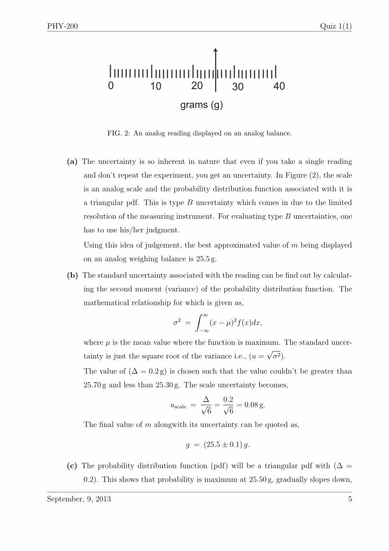
0 10 20 30 40
grams (g)
FIG. 2: An analog reading displayed on an analog balance.
(a) The uncertainty is so inherent in nature that even if you take a single reading
and don’t repeat the experiment, you get an uncertainty. In Figure (2), the scale
is an analog scale and the probability distribution function associated with it is
a triangular pdf. This is type B uncertainty which comes in due to the limited
resolution of the measuring instrument. For evaluating type B uncertainties, one
has to use his/her judgment.
Using this idea of judgement, the best approximated value of m being displayed
on an analog weighing balance is 25.5 g.
(b) The standard uncertainty associated with the reading can be find out by calculat-
ing the second moment (variance) of the probability distribution function. The
mathematical relationship for which is given as,
σ2 =
∫ ∞
−∞(x− µ)2f(x)dx,
where µ is the mean value where the function is maximum. The standard uncer-
tainty is just the square root of the variance i.e., (u =√σ2).
The value of (∆ = 0.2 g) is chosen such that the value couldn’t be greater than
25.70 g and less than 25.30 g. The scale uncertainty becomes,
uscale =∆√6=
0.2√6= 0.08 g.
The final value of m alongwith its uncertainty can be quoted as,
g = (25.5± 0.1) g.
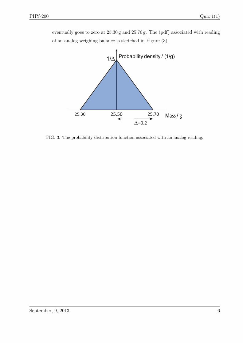
(c) The probability distribution function (pdf) will be a triangular pdf with (∆ =
0.2). This shows that probability is maximum at 25.50 g, gradually slopes down,
September, 9, 2013 5
PHY-200 Quiz 1(1)
eventually goes to zero at 25.30 g and 25.70 g. The (pdf) associated with reading
of an analog weighing balance is sketched in Figure (3).
25.30 25.7025.50 Mass / g
1/∆ Probability density / (1/g)
∆=0.2
FIG. 3: The probability distribution function associated with an analog reading.
September, 9, 2013 6
PHY-200 Quiz 1(2)
Quiz 1(2): Experimental Physics Lab-I
Solution
1. Suppose you measure three numbers as,
x = 20.2 ± 1.5, y = 8.5 ± 0.5, θ = (30 ± 3).
Compute the following expression.
q = x− y sin(θ).
Find the uncertainty in q and quote your results.
Solution:
The value of q is,
q = [20.2− (8.5)(sin 30)] = 15.95 (1)
The uncertainty in q can be calculated using the Taylor series approximation (which
is a general rule),
∆q =
√(∂q
∂x∆x
)2
+
(∂q
∂y∆y
)2
+
(∂q
∂θ∆θ
)2
. (2)
Now differentiating q w.r.t x and multiplying with ∆x yields,(∂q
∂x
)∆x = (1)(1.5) = 1.5 (3)
Likewise, the second quantity of Equation (2) becomes,(∂q
∂y
)∆y = − sin θ∆y = (− sin 30)(0.5),
= (−0.5)(0.5) = −0.25 (4)
and, (∂q
∂θ
)∆θ = (−y cos θ)(∆θ),
= (−8.5× 0.866)
(3π
180
)= 0.3852 (5)
September, 9, 2013 1
PHY-200 Quiz 1(2)
Substituting the values of Equations (3), (4), (5) in Equation (2) yields,
∆q =√
(1.5)2 + (0.25)2 + (0.3852)2 = 1.56 (6)
The final value of q can be quoted as,
q = (16.0± 1.6).
2. To calibrate a prism spectrometer, a student sends light of 10 different known wave-
lengths λ through the spectrometer and measures the angle θ by which each beam
is deflected. For one particular value of λ, the student measures θ seven times and
obtains these results (in degrees).
52.5, 52.3, 52.6, 52.5, 52.7, 52.4, 52.5
(a) Find the best estimated value of θ and its standard uncertainty.
(b) How many measurements would you expect to lie outside the 95% confidence
interval? How many actually do?
Solution:
(a) The mean value of the measured angle θ is,
< θ > =
∑7i=1 θin
=367.5
7= 52.5 (7)
The deviations di can be found out using the following relationship,
di = θi − < θ > . (8)
The calculated deviations of all the measured angles are tabulated in Table (I).
The standard deviation s is,
s =
√∑7i=1 d
2i
n=
√0.1
7= 0.119
and sandard uncertainty is,
σ =
√n
n− 1(s) =
√7
6(0.119) = 0.129
September, 9, 2013 2
PHY-200 Quiz 1(2)
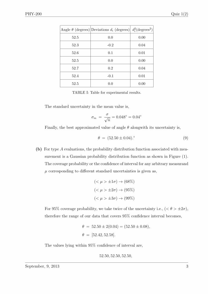
Angle θ (degrees) Deviations di (degrees) d2i (degrees2)
52.5 0.0 0.00
52.3 -0.2 0.04
52.6 0.1 0.01
52.5 0.0 0.00
52.7 0.2 0.04
52.4 -0.1 0.01
52.5 0.0 0.00
TABLE I: Table for experimental results.
The standard uncertainty in the mean value is,
σm =σ√n= 0.048 = 0.04
Finally, the best approximated value of angle θ alongwith its uncertainty is,
θ = (52.50± 0.04). (9)
(b) For type A evaluations, the probability distribution function associated with mea-
surement is a Gaussian probability distribution function as shown in Figure (1).
The coverage probability or the confidence of interval for any arbitrary measurand
µ corresponding to different standard uncertainties is given as,
(< µ > ±1σ) → (68%)
(< µ > ±2σ) → (95%)
(< µ > ±3σ) → (99%)
For 95% coverage probability, we take twice of the uncertainty i.e., (< θ > ±2σ),
therefore the range of our data that covers 95% confidence interval becomes,
θ = 52.50± 2(0.04) = (52.50± 0.08),
θ = [52.42, 52.58].
The values lying within 95% confidence of interval are,
52.50, 52.50, 52.50,
September, 9, 2013 3
PHY-200 Quiz 1(2)
µ µ+σµ−σ
2σ
The shaded area between
µ−σ and µ+σ is 0.68
p(x)
x
of the total area
µ+2σ µ+3σµ−2σµ−3σ
FIG. 1: A Gaussian probability distribution function.
and values lying outside 95% confidence of interval (or within 5%) are,
52.30, 52.40, 52.60, 52.70.
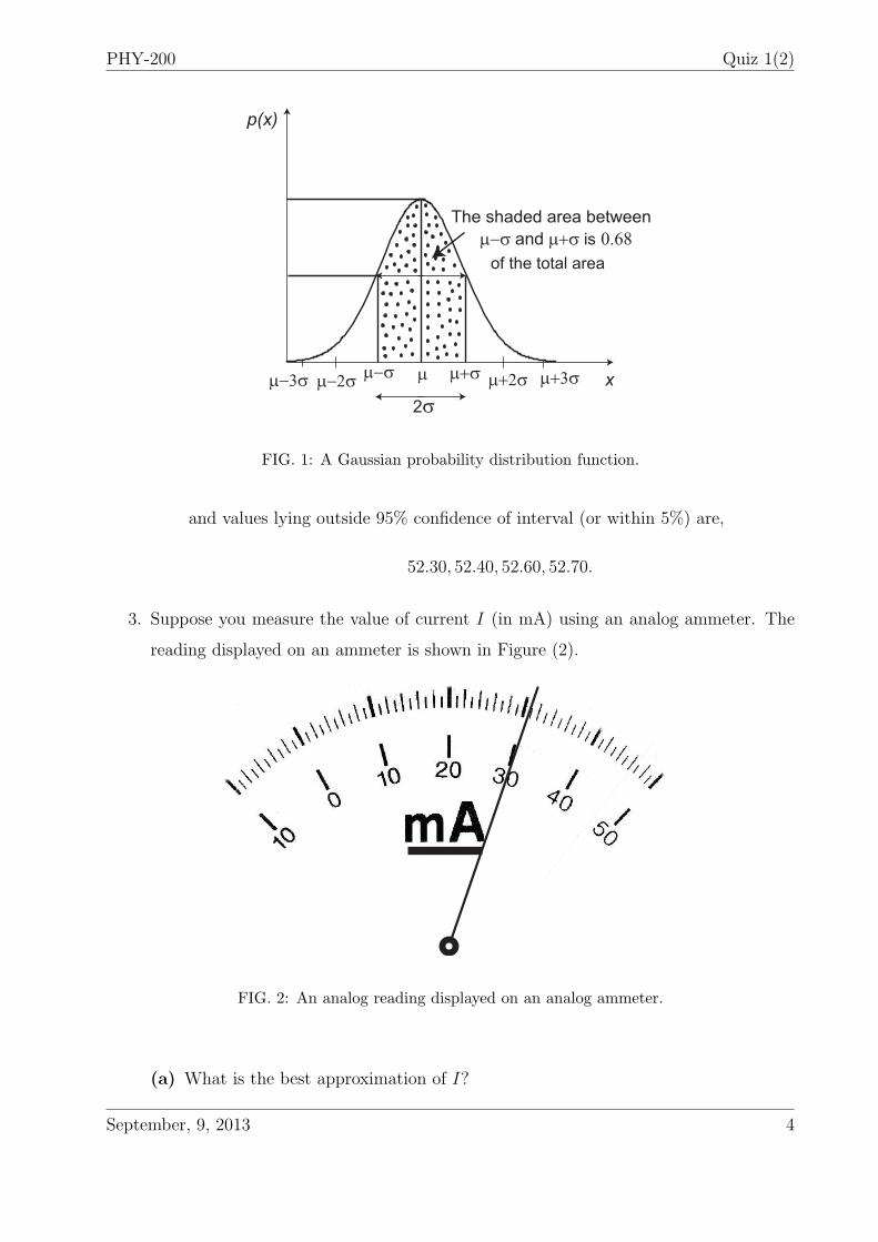
3. Suppose you measure the value of current I (in mA) using an analog ammeter. The
reading displayed on an ammeter is shown in Figure (2).
FIG. 2: An analog reading displayed on an analog ammeter.
(a) What is the best approximation of I?
September, 9, 2013 4
PHY-200 Quiz 1(2)
(b) Find the standard uncertainty associated with the reading?
(c) What probability distribution function did you use to model your knowledge about
I.
Solution:
(a) The uncertainty is so inherent in nature that even if you take a single reading and
don’t repeat the experiment, you get an uncertainty. The scale is an analog scale
in Figure (2) with a triangular probability distribution function associated with
it. This is type B uncertainty which comes in due to the limited resolution of the
measuring instrument. For type B evaluations, one has to use his/her judgment.
Using this idea of judgement, the best approximated value of I being displayed
on an analog ammeter is 30.8mA.
(b) The second moment (variance) of the probability distribution function is a mea-
sure of finding the standard uncertainty. The mathematical relationship for which
is given as,
σ2 =
∫ ∞
−∞(x− µ)2f(x)dx,
and the standard uncertainty is just the square root of the variance i.e., (u =√σ2).
The value of ∆ can be chosen such that the value couldn’t be greater than 31.0mA
and less than 30.6mA. The ∆ for the reading being displayed in Figure (2) would
be 0.2mA. The scale uncertainty becomes,
uscale =∆√6=
0.2√6= 0.08mA.
The final value of I alongwith its uncertainty can be quoted as,
I = (30.8± 0.1)mA.
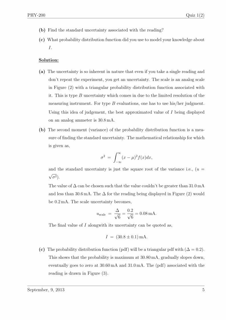
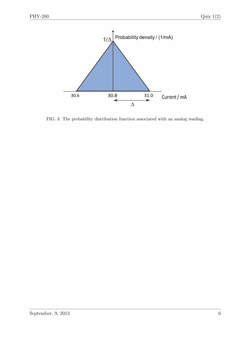
(c) The probability distribution function (pdf) will be a triangular pdf with (∆ = 0.2).
This shows that the probability is maximum at 30.80mA, gradually slopes down,
eventually goes to zero at 30.60mA and 31.0mA. The (pdf) associated with the
reading is drawn in Figure (3).
September, 9, 2013 5
PHY-200 Quiz 1(2)
30.6 31.030.8 Current / mA
1/∆ Probability density / (1/mA)
∆
FIG. 3: The probability distribution function associated with an analog reading.
September, 9, 2013 6
PHY-200 Quiz 2(1)
Quiz 2(1): Experimental Physics Lab-I
Solution
1. A student measures the area of a rectangle several times and concludes the standard
deviation σA of the measurements is σA = 8 cm2. If all the uncertainties are truly
random then the desired precision can be obtained by making enough measurements
and averaging. How many measurements are needed to get a final uncertainty of
±2 cm2. (10 points)
Solution:
The standard deviation of the measured data is σA = 8 cm2.
The standard uncertainty in the mean value can be find out using the following rela-
tionship,
σm =σ√n. (1)
Rearranging the above expression yields,
n =
(σ
σm
)2
,
=
(8
2
)2
= 16.
Hence we conclude that we need to repeat the measurements 16 times to minimize the
final uncertainty upto ±2 cm2.
2. A students wants to measure the spring constant of a spring. For that the student
loads it with various masses m and measures the corresponding lengths l. The mass
is measured using a digital weighing balance (rating= 1%) while lengths is measured
using a ruler. The results are shown in Table (I).
The force is,
mg = k(l − lo), (2)
where lo is the unstretched length of the spring and k is the spring constant. The data
should fit a straight line.
September, 18, 2013 1
PHY-200 Quiz 2(1)
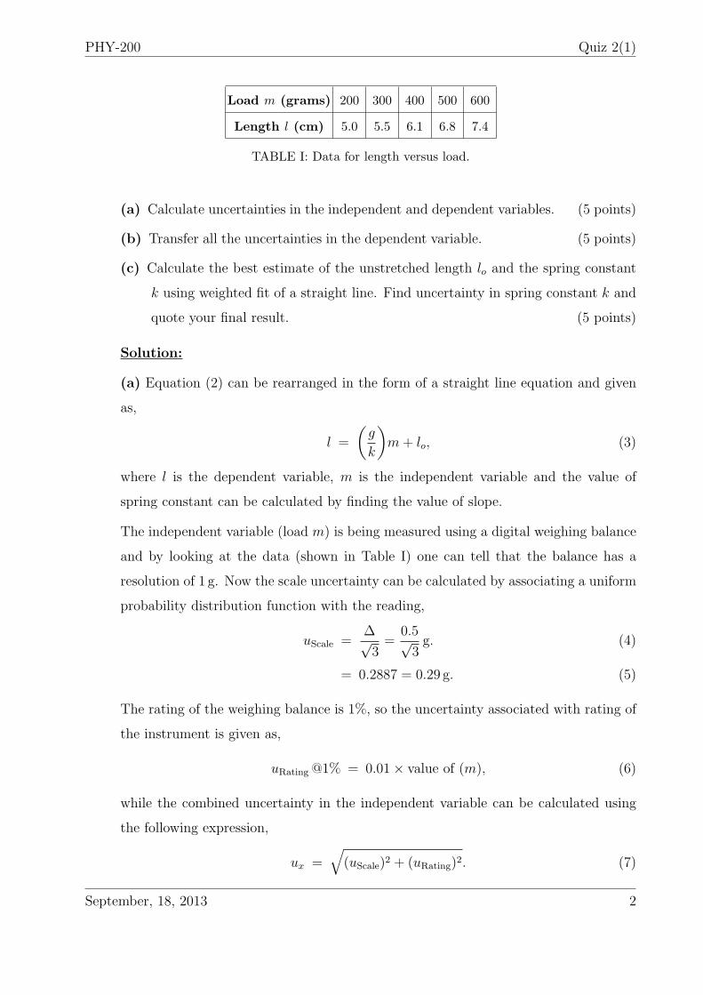
Load m (grams) 200 300 400 500 600
Length l (cm) 5.0 5.5 6.1 6.8 7.4
TABLE I: Data for length versus load.
(a) Calculate uncertainties in the independent and dependent variables. (5 points)
(b) Transfer all the uncertainties in the dependent variable. (5 points)
(c) Calculate the best estimate of the unstretched length lo and the spring constant
k using weighted fit of a straight line. Find uncertainty in spring constant k and
quote your final result. (5 points)
Solution:
(a) Equation (2) can be rearranged in the form of a straight line equation and given
as,
l =
(g
k
)m+ lo, (3)
where l is the dependent variable, m is the independent variable and the value of
spring constant can be calculated by finding the value of slope.
The independent variable (load m) is being measured using a digital weighing balance
and by looking at the data (shown in Table I) one can tell that the balance has a
resolution of 1 g. Now the scale uncertainty can be calculated by associating a uniform
probability distribution function with the reading,
uScale =∆√3=
0.5√3g. (4)
= 0.2887 = 0.29 g. (5)
The rating of the weighing balance is 1%, so the uncertainty associated with rating of
the instrument is given as,
uRating @1% = 0.01× value of (m), (6)
while the combined uncertainty in the independent variable can be calculated using
the following expression,
ux =√
(uScale)2 + (uRating)2. (7)
September, 18, 2013 2
PHY-200 Quiz 2(1)
The uncertainty in the dependent variable (length l) has a triangular probability dis-
tribution function associated with it and can be calculated using judgement. For the
given data, the uncertainty would be,
uy =∆√6=
0.1√6cm. (8)
The uncertainties being quoted in independent and dependent variables are shown in
Table (II).
(b) The mathematical expressions for transferring uncertainties to the dependent vari-
able and for calculating the total uncertainty are,
uTrans =
(dy
dx
)ux = (0.006)ux, (9)
uTotal =√
(uTrans)2 + u2y. (10)
The weights w are reciprocal squares of the total uncertainty which are utilized in
least-squares fitting of a straight line. The expression for calculating the weight w is,
w =1
u2Total
. (11)
Now the uncertainties calculated for the given data of independent (load m) and
dependent (length l) variables are shown in Table (II).
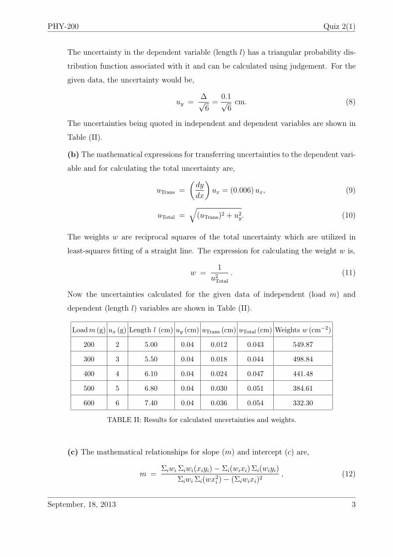
Loadm (g) ux (g) Length l (cm) uy (cm) uTrans (cm) uTotal (cm) Weights w (cm−2)
200 2 5.00 0.04 0.012 0.043 549.87
300 3 5.50 0.04 0.018 0.044 498.84
400 4 6.10 0.04 0.024 0.047 441.48
500 5 6.80 0.04 0.030 0.051 384.61
600 6 7.40 0.04 0.036 0.054 332.30
TABLE II: Results for calculated uncertainties and weights.
(c) The mathematical relationships for slope (m) and intercept (c) are,
m =Σiwi Σiwi(xiyi)− Σi(wixi) Σi(wiyi)
Σiwi Σi(wx2i )− (Σiwixi)2
, (12)
September, 18, 2013 3
PHY-200 Quiz 2(1)
and,
c =Σi(wix
2i ) Σi(wiyi)− Σi(wixi) Σi(wixiyi)
ΣiwiΣi(wix2i )− (Σiwixi)2
, (13)
where x is the independent variable (load m in our case), y is the dependent variable
(length l) and w is the weight.
The different terms in the numerator and denominator of Equations (12) and (13) are
calculated separately and tabulated in Table (III).
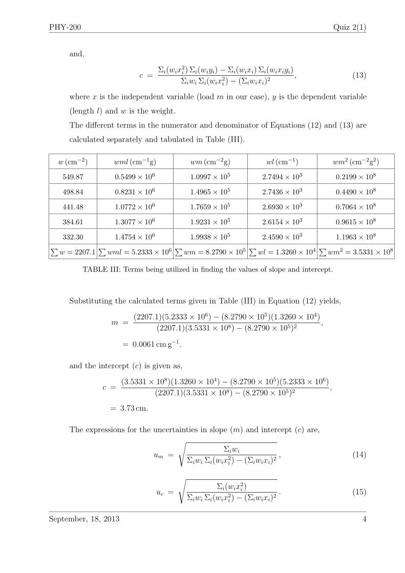
w (cm−2) wml (cm−1g) wm (cm−2g) wl (cm−1) wm2 (cm−2g2)
549.87 0.5499× 10⁶ 1.0997× 10⁵ 2.7494× 10³ 0.2199× 10⁸
498.84 0.8231× 10⁶ 1.4965× 10⁵ 2.7436× 10³ 0.4490× 10⁸
441.48 1.0772× 10⁶ 1.7659× 10⁵ 2.6930× 10³ 0.7064× 10⁸
384.61 1.3077× 10⁶ 1.9231× 10⁵ 2.6154× 10³ 0.9615× 10⁸
332.30 1.4754× 10⁶ 1.9938× 10⁵ 2.4590× 10³ 1.1963× 10⁸∑w = 2207.1
∑wml = 5.2333× 10⁶
∑wm = 8.2790× 10⁵
∑wl = 1.3260× 10⁴
∑wm2 = 3.5331× 10⁸
TABLE III: Terms being utilized in finding the values of slope and intercept.
Substituting the calculated terms given in Table (III) in Equation (12) yields,
m =(2207.1)(5.2333× 10⁶)− (8.2790× 10⁵)(1.3260× 10⁴)
(2207.1)(3.5331× 10⁸)− (8.2790× 10⁵)2,
= 0.0061 cmg−1.
and the intercept (c) is given as,
c =(3.5331× 10⁸)(1.3260× 10⁴)− (8.2790× 10⁵)(5.2333× 10⁶)
(2207.1)(3.5331× 10⁸)− (8.2790× 10⁵)2,
= 3.73 cm.
The expressions for the uncertainties in slope (m) and intercept (c) are,
um =
√Σiwi
ΣiwiΣi(wix2i )− (Σiwixi)2
, (14)
uc =
√Σi(wix2
i )
ΣiwiΣi(wix2i )− (Σiwixi)2
. (15)
September, 18, 2013 4
PHY-200 Quiz 2(1)
Substituting the values yield,
um =
√(2207.1)
(2207.1)(3.5331× 10⁸)− (8.2790× 10⁵)2,
= 1.529× 10⁻⁴ cmg−1. (16)
and expression for finding the uncertainty in the intercept (c) value becomes,
uc =
√(3.5331× 10⁸)
(2207.1)(3.5331× 10⁸)− (8.2790× 10⁵)2,
= 0.0612 cm. (17)
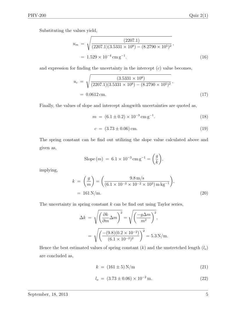
Finally, the values of slope and intercept alongwith uncertainties are quoted as,
m = (6.1± 0.2)× 10−3 cmg−1. (18)
c = (3.73± 0.06) cm. (19)
The spring constant can be find out utilizing the slope value calculated above and
given as,
Slope (m) = 6.1× 10⁻³ cmg−1 =
(g
k
),
implying,
k =
(g
m
)=
(9.8m/s
(6.1× 10−3 × 10−2 × 10³)mkg−1
),
= 161N/m. (20)
The uncertainty in spring constant k can be find out using Taylor series,
∆k =
√(∂k
∂m∆m
)2
=
√(−g∆m
m2
)2
,
=
√(−(9.8)(0.2× 10⁻²)
(6.1× 10⁻²)2
)2
= 5.3N/m.
Hence the best estimated values of spring constant (k) and the unstretched length (lo)
are concluded as,
k = (161± 5)N/m (21)
lo = (3.73± 0.06)× 10−2 m. (22)
September, 18, 2013 5
PHY-200 Quiz 2(2)
Quiz 2(2): Experimental Physics Lab-I
Solution
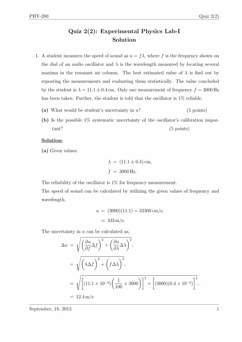
1. A student measures the speed of sound as u = fλ, where f is the frequency shown on
the dial of an audio oscillator and λ is the wavelength measured by locating several
maxima in the resonant air column. The best estimated value of λ is find out by
repeating the measurements and evaluating them statistically. The value concluded
by the student is λ = 11.1± 0.4 cm. Only one measurement of frequency f = 3000Hz
has been taken. Further, the student is told that the oscillator is 1% reliable.
(a) What would be student’s uncertainty in u? (5 points)
(b) Is the possible 1% systematic uncertainty of the oscillator’s calibration impor-
tant? (5 points)
Solution:
(a) Given values:
λ = (11.1± 0.4) cm,
f = 3000Hz.
The reliability of the oscillator is 1% for frequency measurement.
The speed of sound can be calculated by utilizing the given values of frequency and
wavelength.
u = (3000)(11.1) = 33300 cm/s,
= 333m/s.
The uncertainty in u can be calculated as,
∆u =
√(∂u
∂f∆f
)2
+
(∂u
∂λ∆λ
)2
,
=
√(λ∆f
)2
+
(f∆λ
)2
,
=
√[(11.1× 10⁻²)
(1
100× 3000
)]2+
[(3000)(0.4× 10⁻²)
]2,
= 12.4m/s
September, 18, 2013 1
PHY-200 Quiz 2(2)
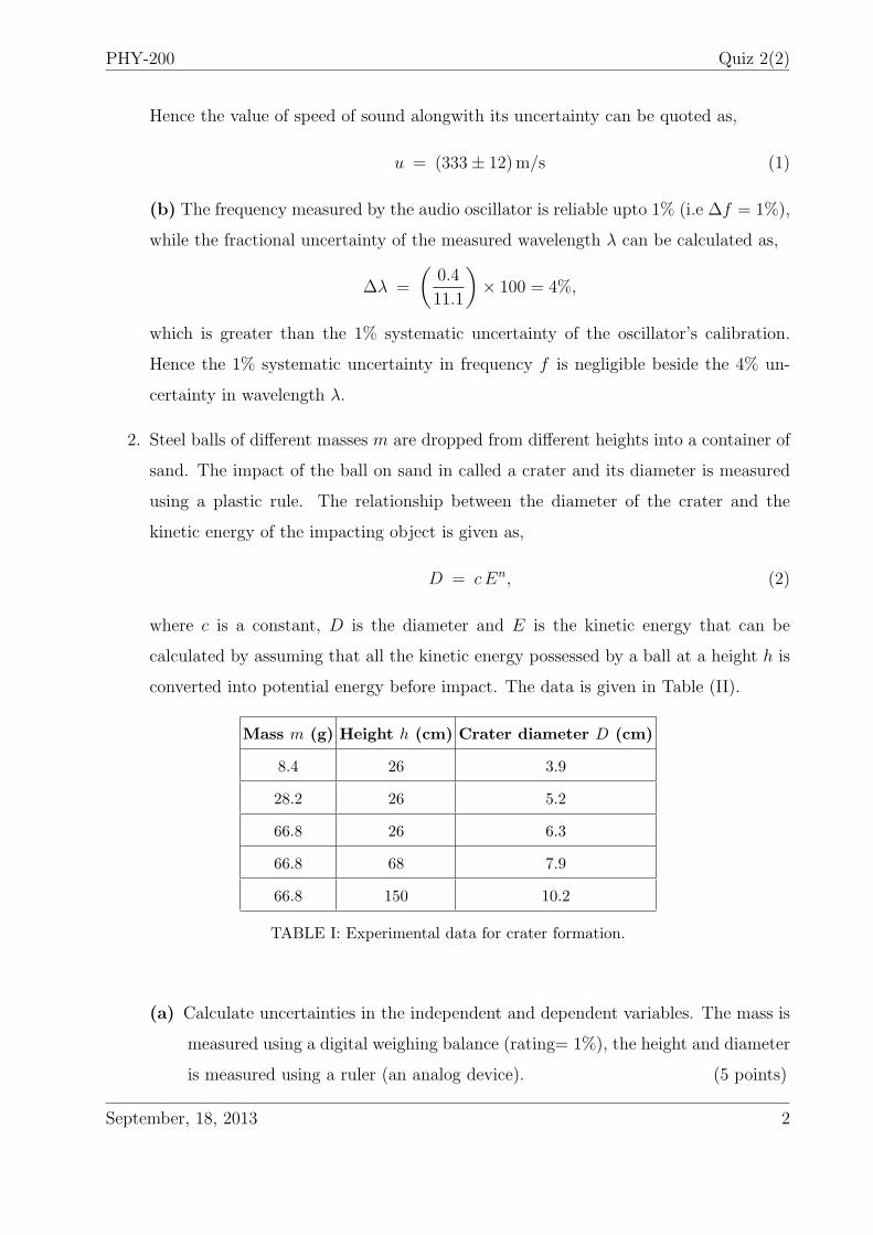
Hence the value of speed of sound alongwith its uncertainty can be quoted as,
u = (333± 12)m/s (1)
(b) The frequency measured by the audio oscillator is reliable upto 1% (i.e ∆f = 1%),
while the fractional uncertainty of the measured wavelength λ can be calculated as,
∆λ =
(0.4
11.1
)× 100 = 4%,
which is greater than the 1% systematic uncertainty of the oscillator’s calibration.
Hence the 1% systematic uncertainty in frequency f is negligible beside the 4% un-
certainty in wavelength λ.
2. Steel balls of different masses m are dropped from different heights into a container of
sand. The impact of the ball on sand in called a crater and its diameter is measured
using a plastic rule. The relationship between the diameter of the crater and the
kinetic energy of the impacting object is given as,
D = cEn, (2)
where c is a constant, D is the diameter and E is the kinetic energy that can be
calculated by assuming that all the kinetic energy possessed by a ball at a height h is
converted into potential energy before impact. The data is given in Table (II).
Mass m (g) Height h (cm) Crater diameter D (cm)
8.4 26 3.9
28.2 26 5.2
66.8 26 6.3
66.8 68 7.9
66.8 150 10.2
TABLE I: Experimental data for crater formation.
(a) Calculate uncertainties in the independent and dependent variables. The mass is
measured using a digital weighing balance (rating= 1%), the height and diameter
is measured using a ruler (an analog device). (5 points)
September, 18, 2013 2
PHY-200 Quiz 2(2)
(b) Using the transformation rule, transfer all the uncertainties to the dependent
variable. (5 points)
(c) Calculate the best estimate of n using weighted fit of a straight line. Calculate
uncertainty in n as well. (5 points)
Solution
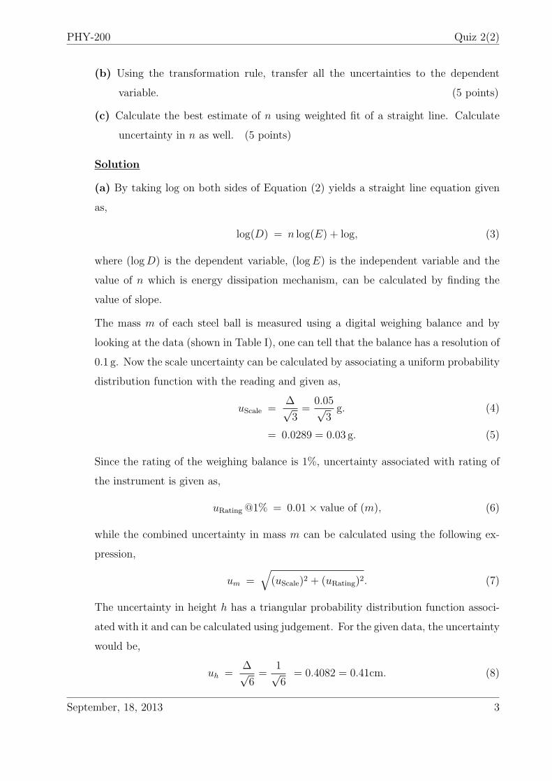
(a) By taking log on both sides of Equation (2) yields a straight line equation given
as,
log(D) = n log(E) + log, (3)
where (logD) is the dependent variable, (logE) is the independent variable and the
value of n which is energy dissipation mechanism, can be calculated by finding the
value of slope.
The mass m of each steel ball is measured using a digital weighing balance and by
looking at the data (shown in Table I), one can tell that the balance has a resolution of
0.1 g. Now the scale uncertainty can be calculated by associating a uniform probability
distribution function with the reading and given as,
uScale =∆√3=
0.05√3g. (4)
= 0.0289 = 0.03 g. (5)
Since the rating of the weighing balance is 1%, uncertainty associated with rating of
the instrument is given as,
uRating @1% = 0.01× value of (m), (6)
while the combined uncertainty in mass m can be calculated using the following ex-
pression,
um =√
(uScale)2 + (uRating)2. (7)
The uncertainty in height h has a triangular probability distribution function associ-
ated with it and can be calculated using judgement. For the given data, the uncertainty
would be,
uh =∆√6=
1√6
= 0.4082 = 0.41cm. (8)
September, 18, 2013 3
PHY-200 Quiz 2(2)
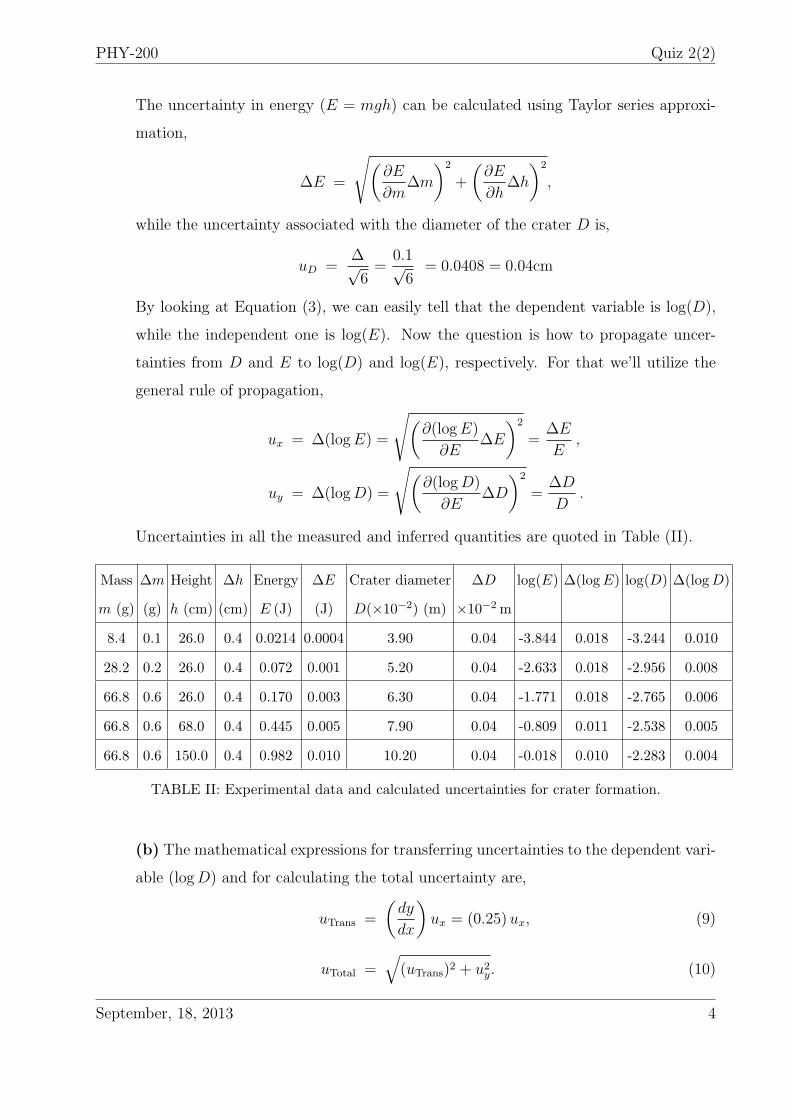
The uncertainty in energy (E = mgh) can be calculated using Taylor series approxi-
mation,
∆E =
√(∂E
∂m∆m
)2
+
(∂E
∂h∆h
)2
,
while the uncertainty associated with the diameter of the crater D is,
uD =∆√6=
0.1√6
= 0.0408 = 0.04cm
By looking at Equation (3), we can easily tell that the dependent variable is log(D),
while the independent one is log(E). Now the question is how to propagate uncer-
tainties from D and E to log(D) and log(E), respectively. For that we’ll utilize the
general rule of propagation,
ux = ∆(logE) =
√(∂(logE)
∂E∆E
)2
=∆E
E,
uy = ∆(logD) =
√(∂(logD)
∂E∆D
)2
=∆D
D.
Uncertainties in all the measured and inferred quantities are quoted in Table (II).
Mass ∆m Height ∆h Energy ∆E Crater diameter ∆D log(E) ∆(logE) log(D) ∆(logD)
m (g) (g) h (cm) (cm) E (J) (J) D(×10−2) (m) ×10−2m
8.4 0.1 26.0 0.4 0.0214 0.0004 3.90 0.04 -3.844 0.018 -3.244 0.010
28.2 0.2 26.0 0.4 0.072 0.001 5.20 0.04 -2.633 0.018 -2.956 0.008
66.8 0.6 26.0 0.4 0.170 0.003 6.30 0.04 -1.771 0.018 -2.765 0.006
66.8 0.6 68.0 0.4 0.445 0.005 7.90 0.04 -0.809 0.011 -2.538 0.005
66.8 0.6 150.0 0.4 0.982 0.010 10.20 0.04 -0.018 0.010 -2.283 0.004
TABLE II: Experimental data and calculated uncertainties for crater formation.
(b) The mathematical expressions for transferring uncertainties to the dependent vari-
able (logD) and for calculating the total uncertainty are,
uTrans =
(dy
dx
)ux = (0.25)ux, (9)
uTotal =√(uTrans)2 + u2
y. (10)
September, 18, 2013 4
PHY-200 Quiz 2(2)
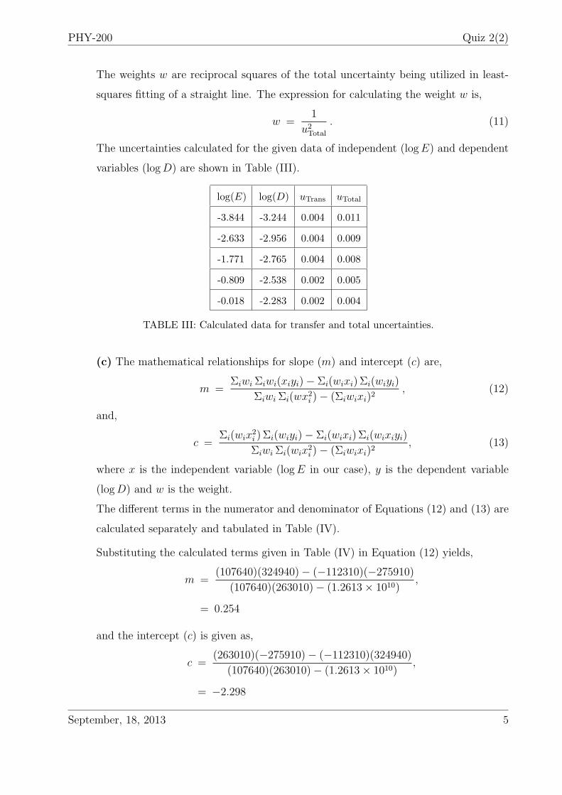
The weights w are reciprocal squares of the total uncertainty being utilized in least-
squares fitting of a straight line. The expression for calculating the weight w is,
w =1
u2Total
. (11)
The uncertainties calculated for the given data of independent (logE) and dependent
variables (logD) are shown in Table (III).
log(E) log(D) uTrans uTotal
-3.844 -3.244 0.004 0.011
-2.633 -2.956 0.004 0.009
-1.771 -2.765 0.004 0.008
-0.809 -2.538 0.002 0.005
-0.018 -2.283 0.002 0.004
TABLE III: Calculated data for transfer and total uncertainties.
(c) The mathematical relationships for slope (m) and intercept (c) are,
m =Σiwi Σiwi(xiyi)− Σi(wixi) Σi(wiyi)
Σiwi Σi(wx2i )− (Σiwixi)2
, (12)
and,
c =Σi(wix
2i ) Σi(wiyi)− Σi(wixi) Σi(wixiyi)
ΣiwiΣi(wix2i )− (Σiwixi)2
, (13)
where x is the independent variable (logE in our case), y is the dependent variable
(logD) and w is the weight.
The different terms in the numerator and denominator of Equations (12) and (13) are
calculated separately and tabulated in Table (IV).
Substituting the calculated terms given in Table (IV) in Equation (12) yields,
m =(107640)(324940)− (−112310)(−275910)
(107640)(263010)− (1.2613× 10¹⁰),
= 0.254
and the intercept (c) is given as,
c =(263010)(−275910)− (−112310)(324940)
(107640)(263010)− (1.2613× 10¹⁰),
= −2.298
September, 18, 2013 5
PHY-200 Quiz 2(2)
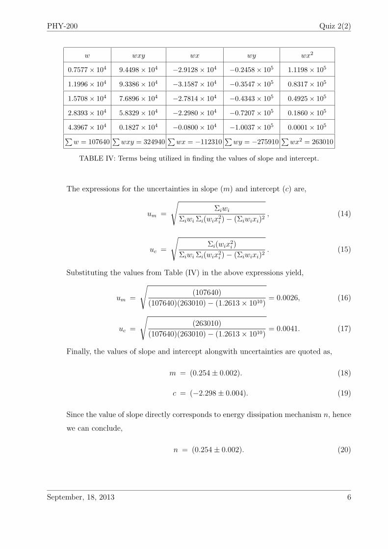
w wxy wx wy wx2
0.7577× 10⁴ 9.4498× 10⁴ −2.9128× 10⁴ −0.2458× 10⁵ 1.1198× 10⁵
1.1996× 10⁴ 9.3386× 10⁴ −3.1587× 10⁴ −0.3547× 10⁵ 0.8317× 10⁵
1.5708× 10⁴ 7.6896× 10⁴ −2.7814× 10⁴ −0.4343× 10⁵ 0.4925× 10⁵
2.8393× 10⁴ 5.8329× 10⁴ −2.2980× 10⁴ −0.7207× 10⁵ 0.1860× 10⁵
4.3967× 10⁴ 0.1827× 10⁴ −0.0800× 10⁴ −1.0037× 10⁵ 0.0001× 10⁵∑w = 107640
∑wxy = 324940
∑wx = −112310
∑wy = −275910
∑wx2 = 263010
TABLE IV: Terms being utilized in finding the values of slope and intercept.
The expressions for the uncertainties in slope (m) and intercept (c) are,
um =
√Σiwi
ΣiwiΣi(wix2i )− (Σiwixi)2
, (14)
uc =
√Σi(wix2
i )
ΣiwiΣi(wix2i )− (Σiwixi)2
. (15)
Substituting the values from Table (IV) in the above expressions yield,
um =
√(107640)
(107640)(263010)− (1.2613× 10¹⁰)= 0.0026, (16)
uc =
√(263010)
(107640)(263010)− (1.2613× 10¹⁰)= 0.0041. (17)
Finally, the values of slope and intercept alongwith uncertainties are quoted as,
m = (0.254± 0.002). (18)
c = (−2.298± 0.004). (19)
Since the value of slope directly corresponds to energy dissipation mechanism n, hence
we can conclude,
n = (0.254± 0.002). (20)
September, 18, 2013 6
PHY-200 Quiz 3
Quiz 3: Experimental Physics Lab-I
Solution
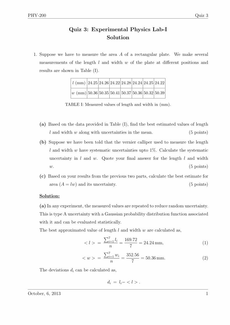
1. Suppose we have to measure the area A of a rectangular plate. We make several
measurements of the length l and width w of the plate at different positions and
results are shown in Table (I).
l (mm) 24.25 24.26 24.22 24.28 24.24 24.25 24.22
w (mm) 50.36 50.35 50.41 50.37 50.36 50.32 50.39
TABLE I: Measured values of length and width in (mm).
(a) Based on the data provided in Table (I), find the best estimated values of length
l and width w along with uncertainties in the mean. (5 points)
(b) Suppose we have been told that the vernier calliper used to measure the length
l and width w have systematic uncertainties upto 1%. Calculate the systematic
uncertainty in l and w. Quote your final answer for the length l and width
w. (5 points)
(c) Based on your results from the previous two parts, calculate the best estimate for
area (A = lw) and its uncertainty. (5 points)
Solution:
(a) In any experiment, the measured values are repeated to reduce random uncertainty.
This is type A uncertainty with a Gaussian probability distribution function associated
with it and can be evaluated statistically.
The best approximated value of length l and width w are calculated as,
< l > =
∑7i=1 lin
=169.72
7= 24.24mm, (1)
< w > =
∑7i=1 wi
n=
352.56
7= 50.36mm. (2)
The deviations di can be calculated as,
di = li− < l > .
October, 6, 2013 1
PHY-200 Quiz 3
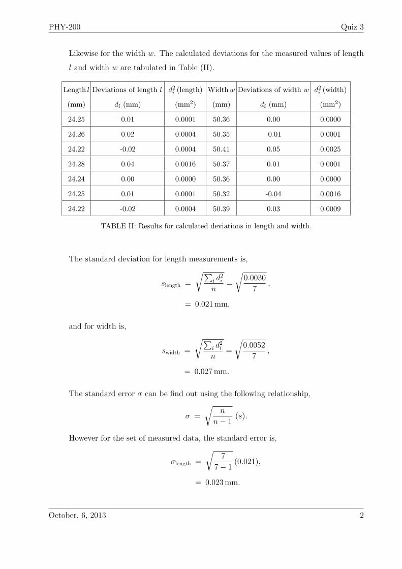
Likewise for the width w. The calculated deviations for the measured values of length
l and width w are tabulated in Table (II).
Length l Deviations of length l d2i (length) Widthw Deviations of width w d2i (width)
(mm) di (mm) (mm2) (mm) di (mm) (mm2)
24.25 0.01 0.0001 50.36 0.00 0.0000
24.26 0.02 0.0004 50.35 -0.01 0.0001
24.22 -0.02 0.0004 50.41 0.05 0.0025
24.28 0.04 0.0016 50.37 0.01 0.0001
24.24 0.00 0.0000 50.36 0.00 0.0000
24.25 0.01 0.0001 50.32 -0.04 0.0016
24.22 -0.02 0.0004 50.39 0.03 0.0009
TABLE II: Results for calculated deviations in length and width.
The standard deviation for length measurements is,
slength =
√∑i d
2i
n=
√0.0030
7,
= 0.021mm,
and for width is,
swidth =
√∑i d
2i
n=
√0.0052
7,
= 0.027mm.
The standard error σ can be find out using the following relationship,
σ =
√n
n− 1(s).
However for the set of measured data, the standard error is,
σlength =
√7
7− 1(0.021),
= 0.023mm.
October, 6, 2013 2
PHY-200 Quiz 3
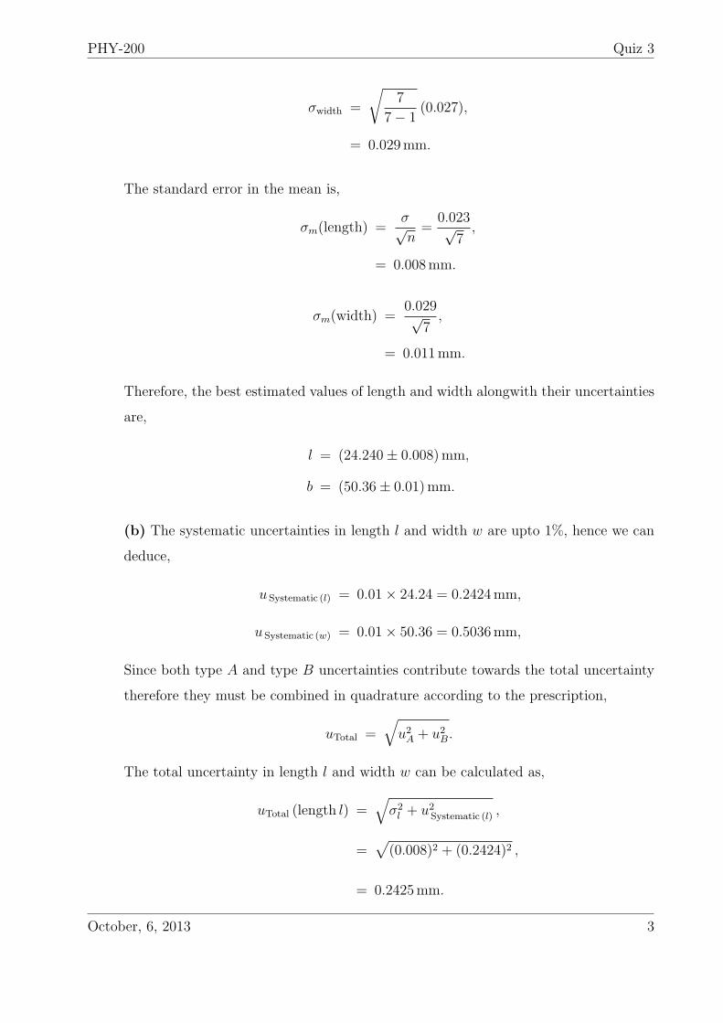
σwidth =
√7
7− 1(0.027),
= 0.029mm.
The standard error in the mean is,
σm(length) =σ√n=
0.023√7
,
= 0.008mm.
σm(width) =0.029√
7,
= 0.011mm.
Therefore, the best estimated values of length and width alongwith their uncertainties
are,
l = (24.240± 0.008)mm,
b = (50.36± 0.01)mm.
(b) The systematic uncertainties in length l and width w are upto 1%, hence we can
deduce,
u Systematic (l) = 0.01× 24.24 = 0.2424mm,
u Systematic (w) = 0.01× 50.36 = 0.5036mm,
Since both type A and type B uncertainties contribute towards the total uncertainty
therefore they must be combined in quadrature according to the prescription,
uTotal =√u2A + u2
B.
The total uncertainty in length l and width w can be calculated as,
uTotal (length l) =√
σ2l + u2
Systematic (l) ,
=√
(0.008)2 + (0.2424)2 ,
= 0.2425mm.
October, 6, 2013 3
PHY-200 Quiz 3
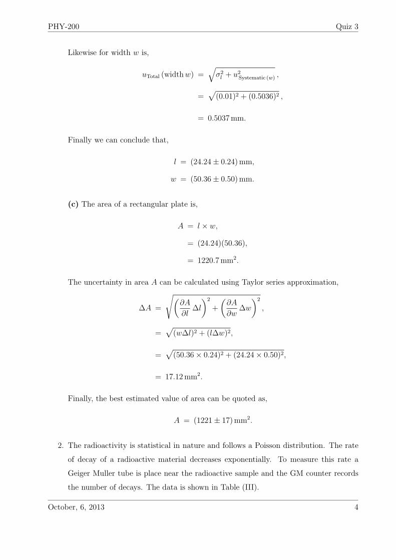
Likewise for width w is,
uTotal (widthw) =√σ2l + u2
Systematic (w) ,
=√(0.01)2 + (0.5036)2 ,
= 0.5037mm.
Finally we can conclude that,
l = (24.24± 0.24)mm,
w = (50.36± 0.50)mm.
(c) The area of a rectangular plate is,
A = l × w,
= (24.24)(50.36),
= 1220.7mm2.
The uncertainty in area A can be calculated using Taylor series approximation,
∆A =
√(∂A
∂l∆l
)2
+
(∂A
∂w∆w
)2
,
=√
(w∆l)2 + (l∆w)2,
=√
(50.36× 0.24)2 + (24.24× 0.50)2,
= 17.12mm2.
Finally, the best estimated value of area can be quoted as,
A = (1221± 17)mm2.
2. The radioactivity is statistical in nature and follows a Poisson distribution. The rate
of decay of a radioactive material decreases exponentially. To measure this rate a
Geiger Muller tube is place near the radioactive sample and the GM counter records
the number of decays. The data is shown in Table (III).
October, 6, 2013 4
PHY-200 Quiz 3
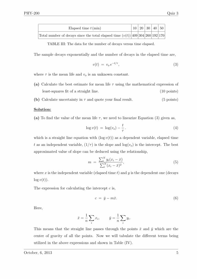
Elapsed time t (min) 10 20 30 40 50
Total number of decays since the total elapsed time (v(t)) 409 304 260 192 170
TABLE III: The data for the number of decays versus time elapsed.
The sample decays exponentially and the number of decays in the elapsed time are,
v(t) = vo e−t/τ , (3)
where τ is the mean life and vo is an unknown constant.
(a) Calculate the best estimate for mean life τ using the mathematical expression of
least-squares fit of a straight line. (10 points)
(b) Calculate uncertainty in τ and quote your final result. (5 points)
Solution:
(a) To find the value of the mean life τ , we need to linearize Equation (3) given as,
log v(t) = log(vo)−t
τ. (4)
which is a straight line equation with (log v(t)) as a dependent variable, elapsed time
t as an independent variable, (1/τ) is the slope and log(vo) is the intercept. The best
approximated value of slope can be deduced using the relationship,
m =
∑Ni yi(xi − x)∑Ni (xi − x)2
, (5)
where x is the independent variable (elapsed time t) and y is the dependent one (decays
log v(t)).
The expression for calculating the intercept c is,
c = y −mx. (6)
Here,
x =1
n
∑i
xi, y =1
n
∑i
yi.
This means that the straight line passes through the points x and y which are the
center of gravity of all the points. Now we will tabulate the different terms being
utilized in the above expressions and shown in Table (IV).
October, 6, 2013 5
PHY-200 Quiz 3
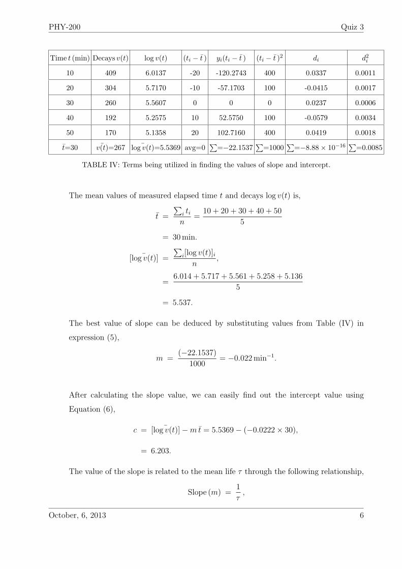
Time t (min) Decays v(t) log v(t) (ti − t ) yi(ti − t ) (ti − t )2 di d2i
10 409 6.0137 -20 -120.2743 400 0.0337 0.0011
20 304 5.7170 -10 -57.1703 100 -0.0415 0.0017
30 260 5.5607 0 0 0 0.0237 0.0006
40 192 5.2575 10 52.5750 100 -0.0579 0.0034
50 170 5.1358 20 102.7160 400 0.0419 0.0018
t=30 ¯v(t)=267 ¯log v(t)=5.5369 avg=0∑
=−22.1537∑
=1000∑
=−8.88× 10⁻¹⁶∑
=0.0085
TABLE IV: Terms being utilized in finding the values of slope and intercept.
The mean values of measured elapsed time t and decays log v(t) is,
t =
∑i tin
=10 + 20 + 30 + 40 + 50
5
= 30min.
[ ¯log v(t)] =
∑i[log v(t)]i
n,
=6.014 + 5.717 + 5.561 + 5.258 + 5.136
5
= 5.537.
The best value of slope can be deduced by substituting values from Table (IV) in
expression (5),
m =(−22.1537)
1000= −0.022min−1.
After calculating the slope value, we can easily find out the intercept value using
Equation (6),
c = [ ¯log v(t)]−m t = 5.5369− (−0.0222× 30),
= 6.203.
The value of the slope is related to the mean life τ through the following relationship,
Slope (m) =1
τ,
October, 6, 2013 6
PHY-200 Quiz 3
implying,
τ =1
(Slope m)=
1
0.022= 45.45min.
(b) The uncertainty in slope can be calculated as,
∆m =
√ ∑Ni d2i
D(N − 2),
where (di = yi −mxi − c) is the deviation of each point from the best fit straight line
called residuals, and (D =∑N
i (xi − x)2).
Substituting values from Table (IV) into the above expression yields,
∆m =
√0.0085
(1000)(5− 2)= 0.002min−1.
Now the uncertainty in the mean life τ can be find out by Taylor series approximation,
∆τ =
√(∂τ
∂m∆m
)2
=
√(−∆m
m2
)2
,
=
√(0.002
(0.022)2
)2
= 4.13min
Hence the final value of mean life τ can be quoted as,
τ = (45± 4)min.
3. Neutrons reflected by a crystal obey Bragg’s law nλ = 2d sin θ, where λ is the de
Broglie wavelength of the neutrons (λ ∝ sin θ), d is the spacing between the reflecting
planes of atoms in the crystal, θ is the angle between the incident (or reflected) neu-
trons and the atomic planes, and n is an integer. If n and d are known, the measured
value of θ for a beam of monochromatic neutrons determines λ, and hence the kinetic
energy E (∝ (momentum)2 ∝ (1/λ2)) of the neutrons. If (θ = (18 ± 1)), what is
the fractional uncertainty in E? (5 points)
Solution:
October, 6, 2013 7
PHY-200 Quiz 3
The wavelength of the neutrons (assuming, n, d = 1) is given as,
λ ∝ sin θ = sin θ = sin(18),
= 0.3090m.
The uncertainty in λ can be calculated using the generic rule,
∆λ =
√(∂λ
∂θ∆θ
)2
= (cos θ)∆θ,
= cos(18)
(1(π)
180
)= (0.9511)(0.0174),
= 0.0166m.
The calculated value of λ can be quoted as,
λ = (0.31± 0.02)m.
The fractional uncertainty in λ is,
∆λ
λ=
0.02
0.31× 100 = 6.5%. (7)
The kinetic energy of the neutrons is
E ∝ (momentum)2 ∝(
1
λ2
),
=
(1
λ2
)=
1
(0.31)2,
= 10.41 J.
The uncertainty in E can be find out using Taylor series and given as,
∆E =
√(∂E
∂λ∆λ
)2
=
√(−2∆λ
λ3
)2
=
√(−2(0.02)
(0.31)3
)2
= 1.346 J.
Hence we conclude,
E = (10.41± 1.3) J.
October, 6, 2013 8

PHY-200 Quiz 3
The fractional uncertainty in energy E is given as,
∆E
E=
1.3
10.41× 100 = 12.5%. (8)
Comparing Equations (7) and (8) yields that fractional uncertainty in E is almost
double than that in the wavelength λ.
October, 6, 2013 9
Experimental Physics-1 (PHY100). Assignment
Assignment : Error analysis and data processing
(Due date: October. 7, 2011, 11 am)
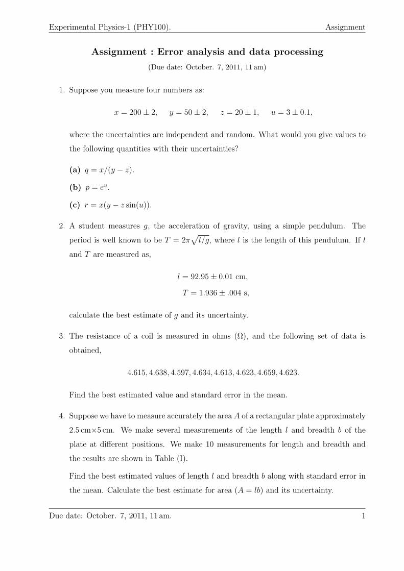
1. Suppose you measure four numbers as:
x = 200± 2, y = 50± 2, z = 20± 1, u = 3± 0.1,
where the uncertainties are independent and random. What would you give values to
the following quantities with their uncertainties?
(a) q = x/(y − z).
(b) p = eu.
(c) r = x(y − z sin(u)).
2. A student measures g, the acceleration of gravity, using a simple pendulum. The
period is well known to be T = 2π√l/g, where l is the length of this pendulum. If l
and T are measured as,
l = 92.95± 0.01 cm,
T = 1.936± .004 s,
calculate the best estimate of g and its uncertainty.
3. The resistance of a coil is measured in ohms (Ω), and the following set of data is
obtained,
4.615, 4.638, 4.597, 4.634, 4.613, 4.623, 4.659, 4.623.
Find the best estimated value and standard error in the mean.
4. Suppose we have to measure accurately the area A of a rectangular plate approximately
2.5 cm×5 cm. We make several measurements of the length l and breadth b of the
plate at different positions. We make 10 measurements for length and breadth and
the results are shown in Table (I).
Find the best estimated values of length l and breadth b along with standard error in
the mean. Calculate the best estimate for area (A = lb) and its uncertainty.
Due date: October. 7, 2011, 11 am. 1
Experimental Physics-1 (PHY100). Assignment
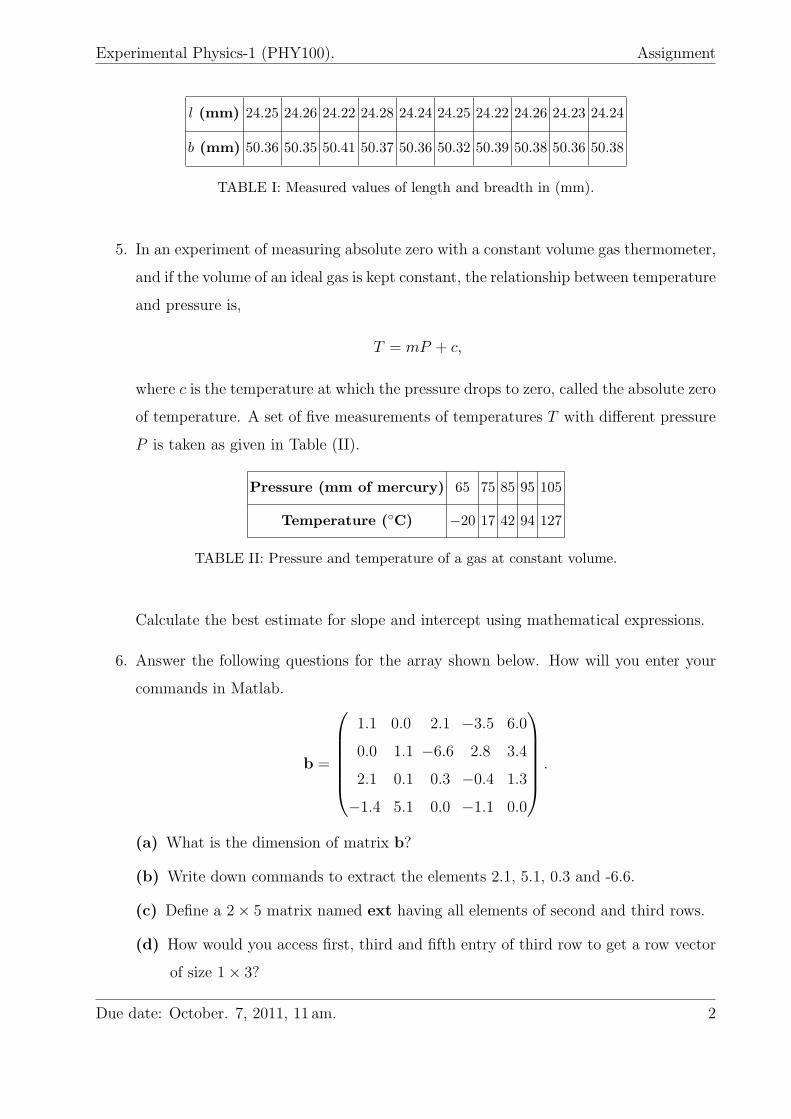
l (mm) 24.25 24.26 24.22 24.28 24.24 24.25 24.22 24.26 24.23 24.24
b (mm) 50.36 50.35 50.41 50.37 50.36 50.32 50.39 50.38 50.36 50.38
TABLE I: Measured values of length and breadth in (mm).
5. In an experiment of measuring absolute zero with a constant volume gas thermometer,
and if the volume of an ideal gas is kept constant, the relationship between temperature
and pressure is,
T = mP + c,
where c is the temperature at which the pressure drops to zero, called the absolute zero
of temperature. A set of five measurements of temperatures T with different pressure
P is taken as given in Table (II).
Pressure (mm of mercury) 65 75 85 95 105
Temperature (C) −20 17 42 94 127
TABLE II: Pressure and temperature of a gas at constant volume.
Calculate the best estimate for slope and intercept using mathematical expressions.
6. Answer the following questions for the array shown below. How will you enter your
commands in Matlab.
b =
1.1 0.0 2.1 −3.5 6.0
0.0 1.1 −6.6 2.8 3.4
2.1 0.1 0.3 −0.4 1.3
−1.4 5.1 0.0 −1.1 0.0
.
(a) What is the dimension of matrix b?
(b) Write down commands to extract the elements 2.1, 5.1, 0.3 and -6.6.
(c) Define a 2× 5 matrix named ext having all elements of second and third rows.
(d) How would you access first, third and fifth entry of third row to get a row vector
of size 1× 3?
Due date: October. 7, 2011, 11 am. 2
Experimental Physics-1 (PHY100). Assignment
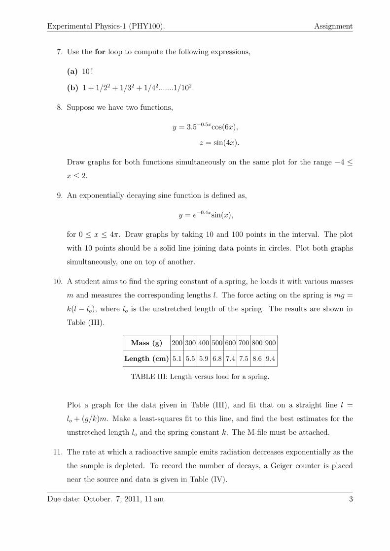
7. Use the for loop to compute the following expressions,
(a) 10 !
(b) 1 + 1/22 + 1/32 + 1/42.......1/102.
8. Suppose we have two functions,
y = 3.5−0.5xcos(6x),
z = sin(4x).
Draw graphs for both functions simultaneously on the same plot for the range −4 ≤
x ≤ 2.
9. An exponentially decaying sine function is defined as,
y = e−0.4xsin(x),
for 0 ≤ x ≤ 4π. Draw graphs by taking 10 and 100 points in the interval. The plot
with 10 points should be a solid line joining data points in circles. Plot both graphs
simultaneously, one on top of another.
10. A student aims to find the spring constant of a spring, he loads it with various masses
m and measures the corresponding lengths l. The force acting on the spring is mg =
k(l − lo), where lo is the unstretched length of the spring. The results are shown in
Table (III).
Mass (g) 200 300 400 500 600 700 800 900
Length (cm) 5.1 5.5 5.9 6.8 7.4 7.5 8.6 9.4
TABLE III: Length versus load for a spring.
Plot a graph for the data given in Table (III), and fit that on a straight line l =
lo + (g/k)m. Make a least-squares fit to this line, and find the best estimates for the
unstretched length lo and the spring constant k. The M-file must be attached.
11. The rate at which a radioactive sample emits radiation decreases exponentially as the
the sample is depleted. To record the number of decays, a Geiger counter is placed
near the source and data is given in Table (IV).
Due date: October. 7, 2011, 11 am. 3
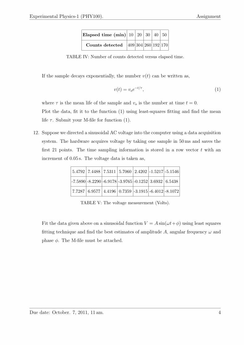
Experimental Physics-1 (PHY100). Assignment
Elapsed time (min) 10 20 30 40 50
Counts detected 409 304 260 192 170
TABLE IV: Number of counts detected versus elapsed time.
If the sample decays exponentially, the number v(t) can be written as,
v(t) = voe−t/τ , (1)
where τ is the mean life of the sample and vo is the number at time t = 0.
Plot the data, fit it to the function (1) using least-squares fitting and find the mean
life τ . Submit your M-file for function (1).
12. Suppose we directed a sinusoidal AC voltage into the computer using a data acquisition
system. The hardware acquires voltage by taking one sample in 50ms and saves the
first 21 points. The time sampling information is stored in a row vector t with an
increment of 0.05 s. The voltage data is taken as,
5.4792 7.4488 7.5311 5.7060 2.4202 -1.5217 -5.1546
-7.5890 -8.2290 -6.9178 -3.9765 -0.1252 3.6932 6.5438
7.7287 6.9577 4.4196 0.7359 -3.1915 -6.4012 -8.1072
TABLE V: The voltage measurement (Volts).
Fit the data given above on a sinusoidal function V = A sin(ωt+ϕ) using least squares
fitting technique and find the best estimates of amplitude A, angular frequency ω and
phase ϕ. The M-file must be attached.
Due date: October. 7, 2011, 11 am. 4
Solution key for error analysis and data processingproblems
Amrozia Shaheen and Muhammad Sabieh AnwarLUMS School of Science and Engineering
October 10, 2011
Q.No.1
Given values of x = 200± 2, y = 50± 2, z = 20± 1 and u = 3± 0.1.
(a)The value of q is,
q =x
(y − z)=
200
(50− 20)= 6.66.
Let’s define a function a,
a = y − z.
The uncertainty in a is,
∆a =√(∆y)2 + (∆z)2,
=√(2)2 + (1)2,
= 2.24 ≈ 2.
Therefore,
a = (30± 2).
The error in q is,
∆q
q=
√(∆x
x
)2
+
(∆a
a
)2
,
∆q = q
√(2
200
)2
+
(2
30
)2
,
= 0.45.
Hence,
q = (6.6± 0.5).
1
(b)Many calculations require complicated operations such as computation of sine,cosine, exponential or square root. In such cases the uncertainties can be calculatedby taking the partial derivative and multiplying with the uncertainty.
Suppose we have a function p,
p = eu.
The uncertainty in p can be calculated using the relationship,
(∆p)2 =
(dp
du
)2
(∆u)2.
Implying,
∆p = eu∆u,
= e3(0.1),
= 2.01.
The value of p is,
p = e3 = 20.08.
Now we can write,
p = (20± 2)
(c) The value of r is,
r = x (y − z sin(u)),
= 200 (50− (20 sin(3))),
= 97990.6
Let’s define a function b as,
b = sin(u).
The uncertainty in b is,
∆b =
(db
du
)∆u,
= cos(u)∆u,
= cos(3)(0.1
57.3) = 1.74× 10⁻³,
= 0.002.
The value of b is,
b = 0.052.
2
So,
b = (0.052± 0.002).
Suppose we take,
c = z b,
and its value is,
c = (20)(0.052) = 1.04.
The error in c is,(∆c
c
)=
√(∆z
z
)2
+
(∆b
b
)2
,
∆c = c
√(1
20
)2
+
(0.002
0.052
)2
= (1.04)(0.063),
= 0.07.
Therefore,
c = (1.04± 0.07).
Now,
d = y − c.
The value of c is calculated as,
d = 50− 1.04 = 48.96.
The uncertainty in d is,
∆d =√
(∆y)2 + (∆c)2,
=√
(2)2 + (0.07)2,
= 2.
Implies that,
d = (49± 2).
Now the function r can be written as,
r = x d.
The uncertainty in r is,(∆r
r
)=
√(∆x
x
)2
+
(∆d
d
)2
,
∆r = r
√(2
200
)2
+
(2
49
)2
,
= 4115.6.
3
Hence we can write,
r = (97991± 4116).
Q.No.2
The time period of a simple pendulum is given as,
T = 2π
√l
g. (1)
The best estimates of l and T are,
l = 92.95± 0.01 cm,
T = 1.936± 0.004 s.
We can find g by rearranging Equation (1),
g = 4π2l/T 2,
and its best estimated value is,
g =4π2 × (92.95 cm)
(1.936 s)2= 979 cm/s2.
If the various uncertainties are independent and random, the fractional uncertaintyin g is just the quadratic sum of the fractional uncertainties of l and T , given as,(
∆g
g
)=
√(∆l
l
)2
+
(2∆T
T
)2
,
∆g = g
√(0.01
92.95
)2
+
(20.004
1.936
)2
,
= 4.04
Thus, based on these measurements, our final answer is,
g = (979± 4) cm/s2
Q.No.3
The mean of the resistance of a coil is,
x =
∑i xi
n
=4.615 + 4.638 + 4.597 + 4.634 + 4.613 + 4.623 + 4.659 + 4.623
8= 4.625Ω.
Deviation from the mean value is,
di = xi − x,
4
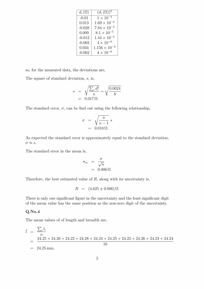
di (Ω) (di (Ω))2
-0.01 1× 10⁻⁴
0.013 1.69× 10⁻⁴
-0.028 7.84× 10⁻⁴
0.009 8.1× 10⁻⁵
-0.012 1.44× 10⁻⁴
-0.002 4× 10⁻⁶
0.034 1.156× 10⁻³
-0.002 4× 10⁻⁶
so, for the measured data, the deviations are,
The square of standard deviation, s, is,
s =
√∑i d
2i
n=
√0.0024
8= 0.017Ω.
The standard error, σ, can be find out using the following relationship,
σ =
√n
n− 1s
= 0.018Ω.
As expected the standard error is approximately equal to the standard deviation,σ ≈ s.
The standard error in the mean is,
σm =σ√n
= 0.006Ω.
Therefore, the best estimated value of R, along with its uncertainty is,
R = (4.625± 0.006)Ω.
There is only one significant figure in the uncertainty and the least significant digitof the mean value has the same position as the non-zero digit of the uncertainty.
Q.No.4
The mean values of of length and breadth are,
l =
∑i lin
=24.25 + 24.26 + 24.22 + 24.28 + 24.24 + 24.25 + 24.22 + 24.26 + 24.23 + 24.24
10= 24.25mm,
5
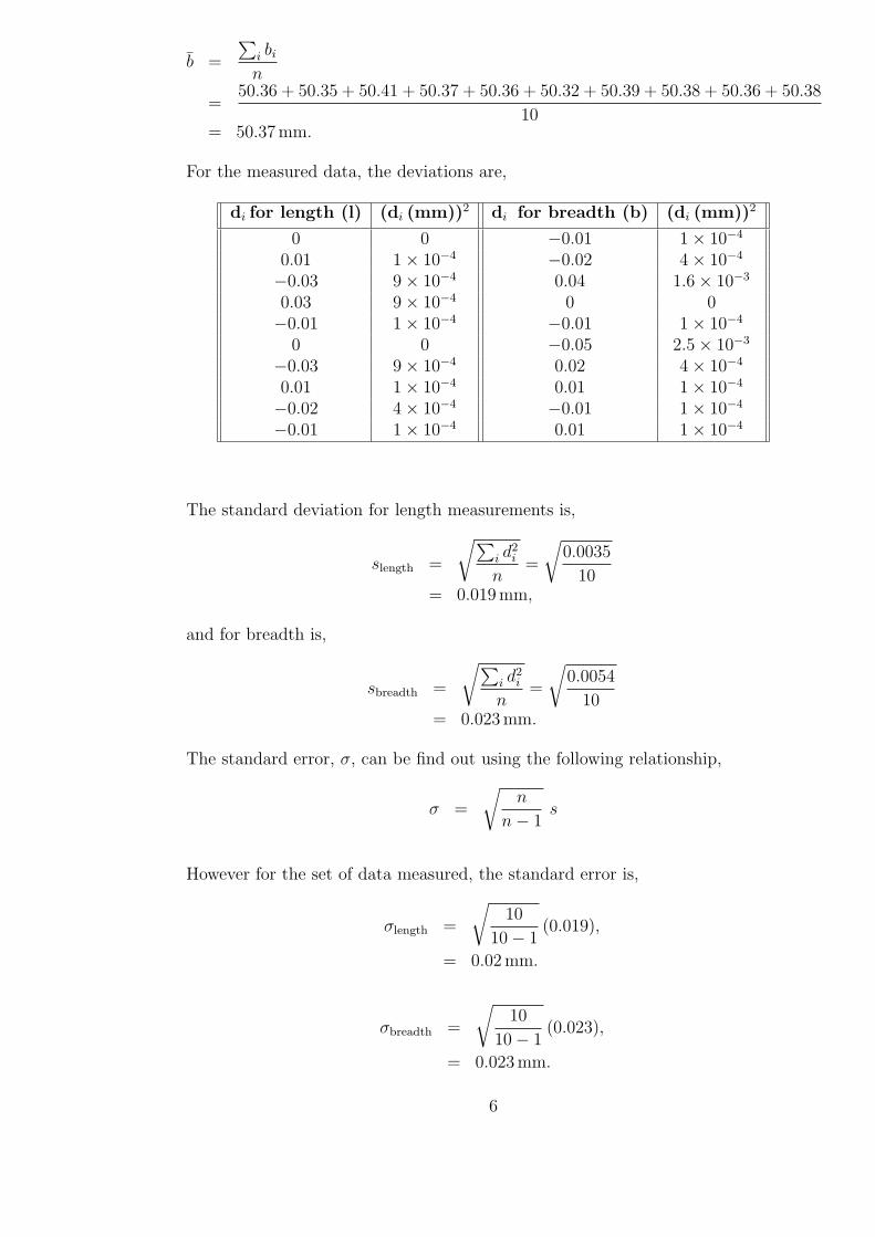
b =
∑i bin
=50.36 + 50.35 + 50.41 + 50.37 + 50.36 + 50.32 + 50.39 + 50.38 + 50.36 + 50.38
10= 50.37mm.
For the measured data, the deviations are,
di for length (l) (di (mm))2 di for breadth (b) (di (mm))2
0 0 −0.01 1× 10⁻⁴
0.01 1× 10⁻⁴ −0.02 4× 10⁻⁴
−0.03 9× 10⁻⁴ 0.04 1.6× 10⁻³
0.03 9× 10⁻⁴ 0 0−0.01 1× 10⁻⁴ −0.01 1× 10⁻⁴
0 0 −0.05 2.5× 10⁻³
−0.03 9× 10⁻⁴ 0.02 4× 10⁻⁴
0.01 1× 10⁻⁴ 0.01 1× 10⁻⁴
−0.02 4× 10⁻⁴ −0.01 1× 10⁻⁴
−0.01 1× 10⁻⁴ 0.01 1× 10⁻⁴
The standard deviation for length measurements is,
slength =
√∑i d
2i
n=
√0.0035
10= 0.019mm,
and for breadth is,
sbreadth =
√∑i d
2i
n=
√0.0054
10= 0.023mm.
The standard error, σ, can be find out using the following relationship,
σ =
√n
n− 1s
However for the set of data measured, the standard error is,
σlength =
√10
10− 1(0.019),
= 0.02mm.
σbreadth =
√10
10− 1(0.023),
= 0.023mm.
6
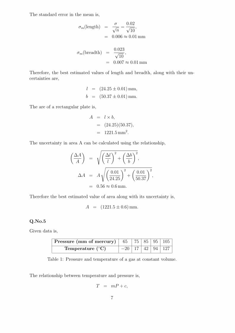
The standard error in the mean is,
σm(length) =σ√n=
0.02√10
,
= 0.006 ≈ 0.01mm
σm(breadth) =0.023√
10,
= 0.007 ≈ 0.01mm
Therefore, the best estimated values of length and breadth, along with their un-certainties are,
l = (24.25± 0.01)mm,
b = (50.37± 0.01)mm.
The are of a rectangular plate is,
A = l × b,
= (24.25)(50.37),
= 1221.5mm2.
The uncertainty in area A can be calculated using the relationship,(∆A
A
)=
√(∆l
l
)2
+
(∆b
b
)2
,
∆A = A
√(0.01
24.25
)2
+
(0.01
50.37
)2
,
= 0.56 ≈ 0.6mm.
Therefore the best estimated value of area along with its uncertainty is,
A = (1221.5± 0.6)mm.
Q.No.5
Given data is,
Pressure (mm of mercury) 65 75 85 95 105
Temperature (C) −20 17 42 94 127
Table 1: Pressure and temperature of a gas at constant volume.
The relationship between temperature and pressure is,
T = mP + c,
7
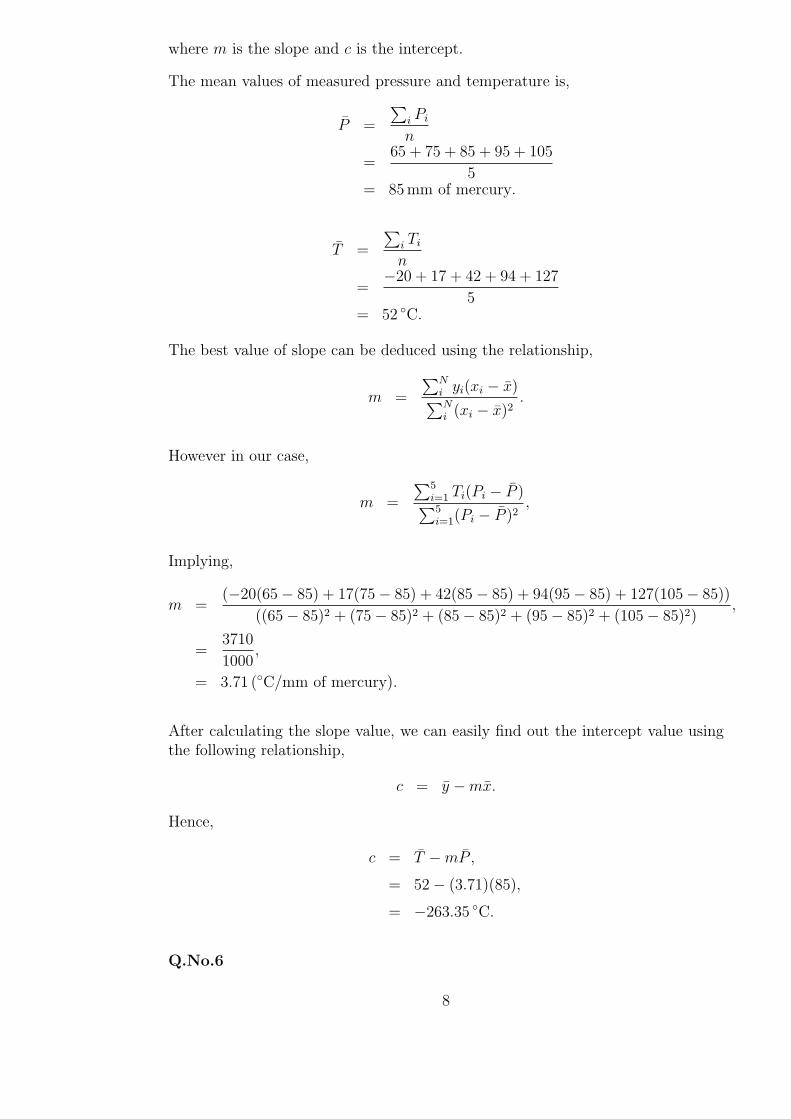
where m is the slope and c is the intercept.
The mean values of measured pressure and temperature is,
P =
∑i Pi
n
=65 + 75 + 85 + 95 + 105
5= 85mm of mercury.
T =
∑i Ti
n
=−20 + 17 + 42 + 94 + 127
5= 52 C.
The best value of slope can be deduced using the relationship,
m =
∑Ni yi(xi − x)∑Ni (xi − x)2
.
However in our case,
m =
∑5i=1 Ti(Pi − P )∑5i=1(Pi − P )2
,
Implying,
m =(−20(65− 85) + 17(75− 85) + 42(85− 85) + 94(95− 85) + 127(105− 85))
((65− 85)2 + (75− 85)2 + (85− 85)2 + (95− 85)2 + (105− 85)2),
=3710
1000,
= 3.71 (C/mm of mercury).
After calculating the slope value, we can easily find out the intercept value usingthe following relationship,
c = y −mx.
Hence,
c = T −mP ,
= 52− (3.71)(85),
= −263.35 C.
Q.No.6
8
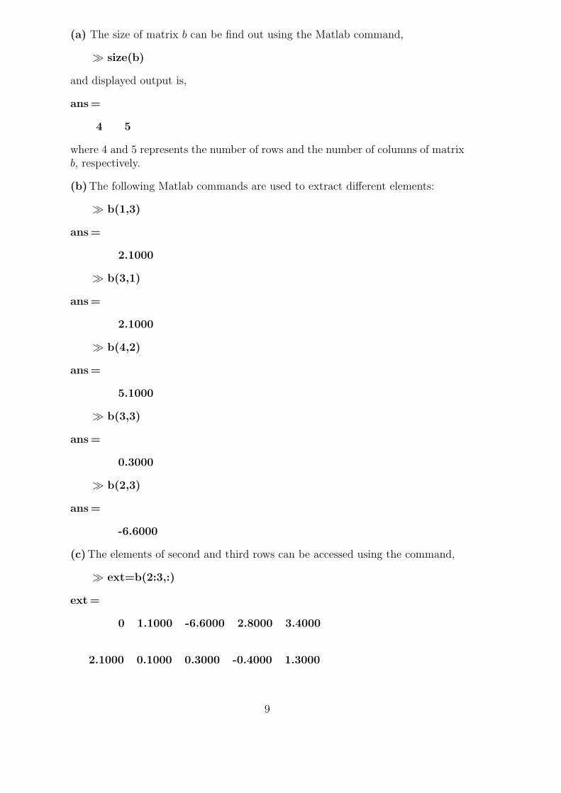
(a) The size of matrix b can be find out using the Matlab command,
≫ size(b)
and displayed output is,
ans=
4 5
where 4 and 5 represents the number of rows and the number of columns of matrixb, respectively.
(b)The following Matlab commands are used to extract different elements:
≫ b(1,3)
ans=
2.1000
≫ b(3,1)
ans=
2.1000
≫ b(4,2)
ans=
5.1000
≫ b(3,3)
ans=
0.3000
≫ b(2,3)
ans=
-6.6000
(c)The elements of second and third rows can be accessed using the command,
≫ ext=b(2:3,:)
ext=
0 1.1000 -6.6000 2.8000 3.4000
2.1000 0.1000 0.3000 -0.4000 1.3000
9
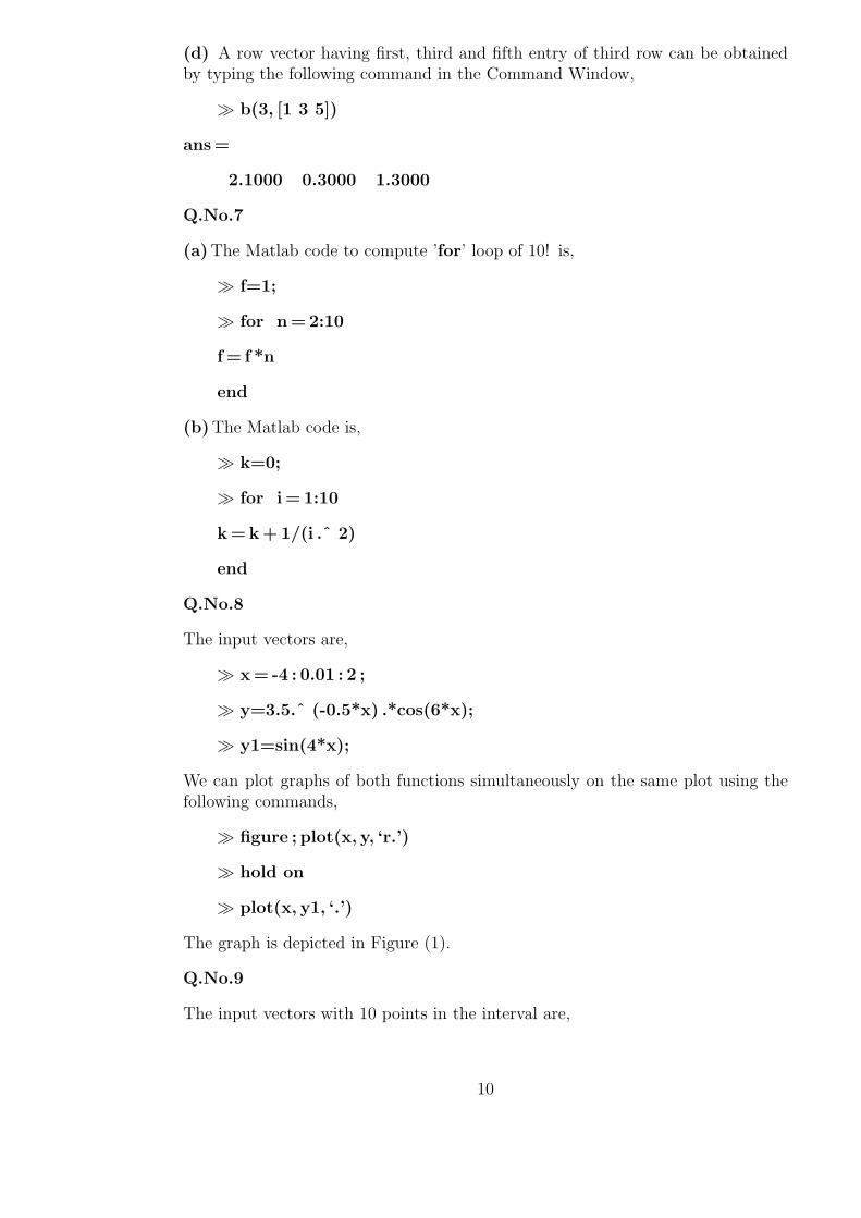
(d) A row vector having first, third and fifth entry of third row can be obtainedby typing the following command in the Command Window,
≫ b(3, [1 3 5])
ans=
2.1000 0.3000 1.3000
Q.No.7
(a)The Matlab code to compute ’for’ loop of 10! is,
≫ f=1;
≫ for n=2:10
f= f *n
end
(b)The Matlab code is,
≫ k=0;
≫ for i= 1:10
k=k+1/(i .ˆ 2)
end
Q.No.8
The input vectors are,
≫ x= -4 : 0.01 : 2 ;
≫ y=3.5.ˆ (-0.5*x) .*cos(6*x);
≫ y1=sin(4*x);
We can plot graphs of both functions simultaneously on the same plot using thefollowing commands,
≫ figure ; plot(x, y, ‘r.’)
≫ hold on
≫ plot(x, y1, ‘.’)
The graph is depicted in Figure (1).
Q.No.9
The input vectors with 10 points in the interval are,
10
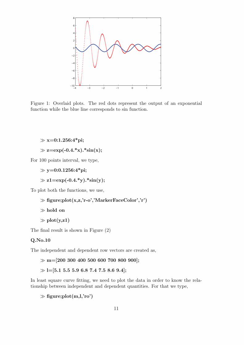
−4 −3 −2 −1 0 1 2−10
−8
−6
−4
−2
0
2
4
6
8
Figure 1: Overlaid plots. The red dots represent the output of an exponentialfunction while the blue line corresponds to sin function.
≫ x=0:1.256:4*pi;
≫ z=exp(-0.4.*x).*sin(x);
For 100 points interval, we type,
≫ y=0:0.1256:4*pi;
≫ z1=exp(-0.4.*y).*sin(y);
To plot both the functions, we use,
≫ figure;plot(x,z,’r-o’,’MarkerFaceColor’,’r’)
≫ hold on
≫ plot(y,z1)
The final result is shown in Figure (2)
Q.No.10
The independent and dependent row vectors are created as,
≫ m=[200 300 400 500 600 700 800 900];
≫ l=[5.1 5.5 5.9 6.8 7.4 7.5 8.6 9.4];
In least square curve fitting, we need to plot the data in order to know the rela-tionship between independent and dependent quantities. For that we type,
≫ figure;plot(m,l,’ro’)
11
0 2 4 6 8 10 12 14−0.2
−0.1
0
0.1
0.2
0.3
0.4
0.5
0.6
Figure 2: An exponentially decaying function. The red line with circles is for 10points in the given interval while blue one is for 100 points.
The data plot shows that our best fit is of the form,
y = mx+ c,
where m is the slope and c is the intercept.
Now we will make an M-file named spring depicted in Figure (3a).
Once the fitting function has been defined, we can find the least squares curveusing the command,
≫ lsqcurvefit(@spring, [3 6.428e-3],m, l)
After the Matlab returns the values of the parameters, the output function isredefined as,
≫ cfit= 3.6857+0.0061*m;
Now we plot the redefined function on the data points using the command,
≫ hold on
≫ plot(m,cfit)
Q.No.11
The input vectors are defined as,
≫ time=[10 20 30 40 50];
≫ counts=[409 304 260 192 170];
The experimental data is plotted using the command,
12
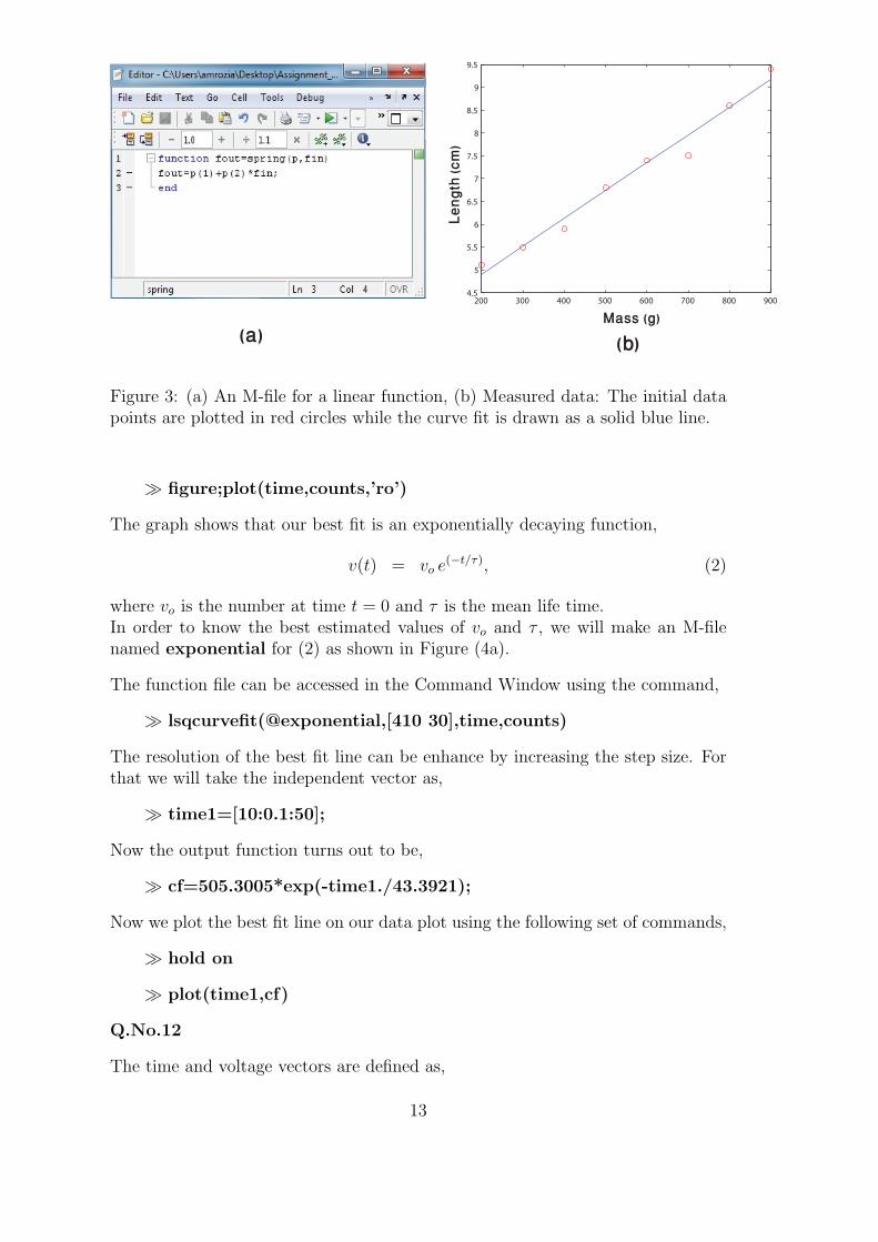
200 300 400 500 600 700 800 9004.5
5
5.5
6
6.5
7
7.5
8
8.5
9
9.5
(a) (b)
Mass (g)
Le
ng
th (
cm
)
Figure 3: (a) An M-file for a linear function, (b) Measured data: The initial datapoints are plotted in red circles while the curve fit is drawn as a solid blue line.
≫ figure;plot(time,counts,’ro’)
The graph shows that our best fit is an exponentially decaying function,
v(t) = vo e(−t/τ), (2)
where vo is the number at time t = 0 and τ is the mean life time.In order to know the best estimated values of vo and τ , we will make an M-filenamed exponential for (2) as shown in Figure (4a).
The function file can be accessed in the Command Window using the command,
≫ lsqcurvefit(@exponential,[410 30],time,counts)
The resolution of the best fit line can be enhance by increasing the step size. Forthat we will take the independent vector as,
≫ time1=[10:0.1:50];
Now the output function turns out to be,
≫ cf=505.3005*exp(-time1./43.3921);
Now we plot the best fit line on our data plot using the following set of commands,
≫ hold on
≫ plot(time1,cf)
Q.No.12
The time and voltage vectors are defined as,
13
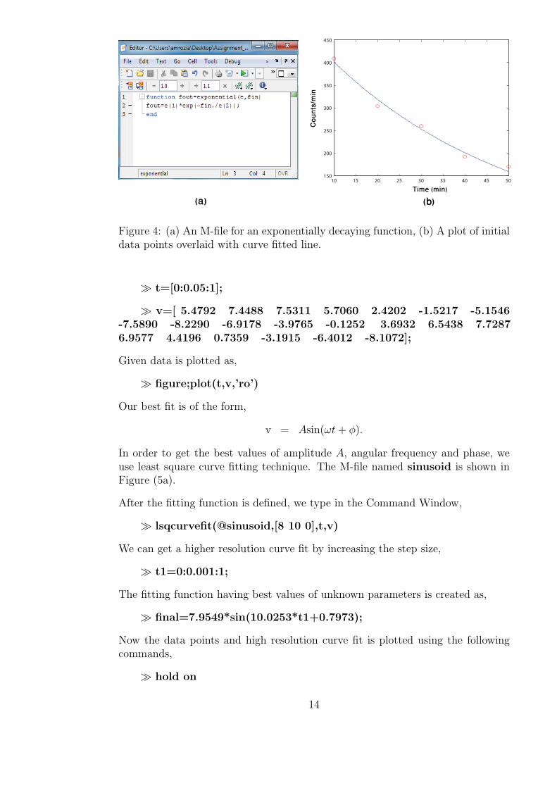
10 15 20 25 30 35 40 45 50150
200
250
300
350
400
450
Time (min)
Co
un
ts/m
in
(a) (b)
Figure 4: (a) An M-file for an exponentially decaying function, (b) A plot of initialdata points overlaid with curve fitted line.
≫ t=[0:0.05:1];
≫ v=[ 5.4792 7.4488 7.5311 5.7060 2.4202 -1.5217 -5.1546-7.5890 -8.2290 -6.9178 -3.9765 -0.1252 3.6932 6.5438 7.72876.9577 4.4196 0.7359 -3.1915 -6.4012 -8.1072];
Given data is plotted as,
≫ figure;plot(t,v,’ro’)
Our best fit is of the form,
v = Asin(ωt+ ϕ).
In order to get the best values of amplitude A, angular frequency and phase, weuse least square curve fitting technique. The M-file named sinusoid is shown inFigure (5a).
After the fitting function is defined, we type in the Command Window,
≫ lsqcurvefit(@sinusoid,[8 10 0],t,v)
We can get a higher resolution curve fit by increasing the step size,
≫ t1=0:0.001:1;
The fitting function having best values of unknown parameters is created as,
≫ final=7.9549*sin(10.0253*t1+0.7973);
Now the data points and high resolution curve fit is plotted using the followingcommands,
≫ hold on
14
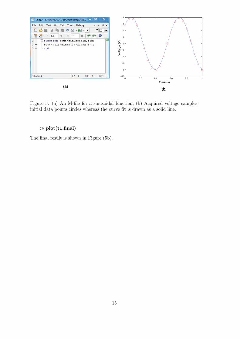
0 0.2 0.4 0.6 0.8 1−10
−8
−6
−4
−2
0
2
4
6
8
Time (s)
Vo
lta
ge
(V
)
(a)(b)
Figure 5: (a) An M-file for a sinusoidal function, (b) Acquired voltage samples:initial data points circles whereas the curve fit is drawn as a solid line.
≫ plot(t1,final)
The final result is shown in Figure (5b).
15