assimilation of soil moisture and land surface temperature ... · pdf fileoutline motivation...
TRANSCRIPT
Assimilation of Soil Moisture and Land Surface Temperature with
the Ensemble Kalman Filter
Workshop on Predictability, Observations, and Uncertainties in GeosciencesFlorida State University
March 13-15, 2006
Rolf Reichle1,2
Mike Bosilovich1
Randy Koster1
Ping Liu1,3
Sarith Mahanama1,2
Jon Radokovich1,3
1 – Global Modeling and Assimilation Office, NASA2 – GEST, University of Maryland, Baltimore County3 – SAIC
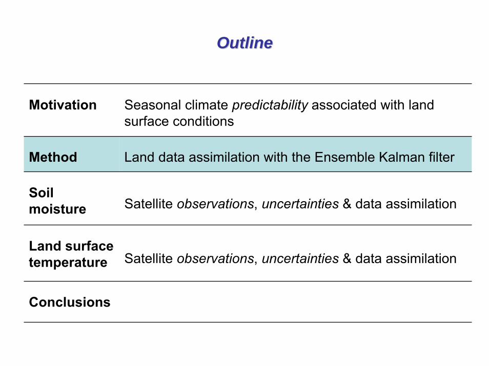
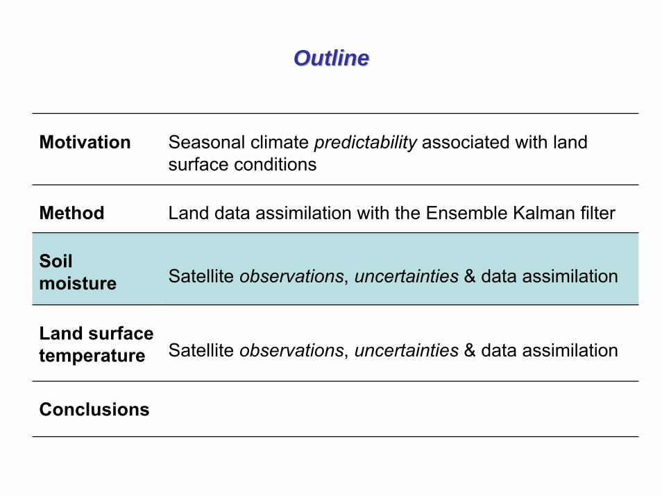
OutlineOutline
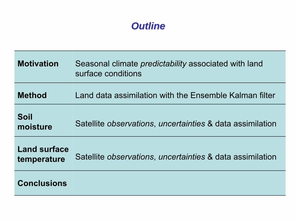
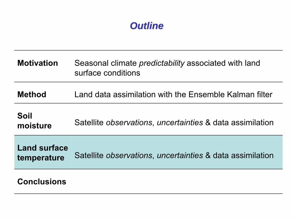
Motivation Seasonal climate predictability associated with land surface conditions
Method Land data assimilation with the Ensemble Kalman filter
Soil moisture Satellite observations, uncertainties & data assimilation
Land surface temperature Satellite observations, uncertainties & data assimilation
Conclusions
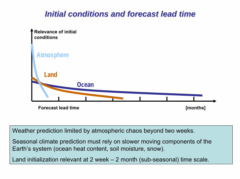
Initial conditions and forecast lead timeInitial conditions and forecast lead time
Relevance of initial conditions
OceanLand
Atmosphere
Forecast lead time [months]
Weather prediction limited by atmospheric chaos beyond two weeks.
Seasonal climate prediction must rely on slower moving components of the Earth’s system (ocean heat content, soil moisture, snow).
Land initialization relevant at 2 week – 2 month (sub-seasonal) time scale.

A simple view of landA simple view of land--atmosphere feedbackatmosphere feedback
…causing soilmoisture toincrease...
…which affects the overlying atmosphere (the boundary layer structure, humidity, etc.)...
Precipitation wets thesurface...
…which causesevaporation to increase duringsubsequent daysand weeks...
…thereby (maybe) inducing additional precipitation
Perhaps such feedback contributes to predictability?Two things must happen:1. A soil moisture anomaly must be “remembered” into the forecast period. 2. The atmosphere must respond predictably to soil moisture anomalies.In other words, need strong land-atmosphere coupling…
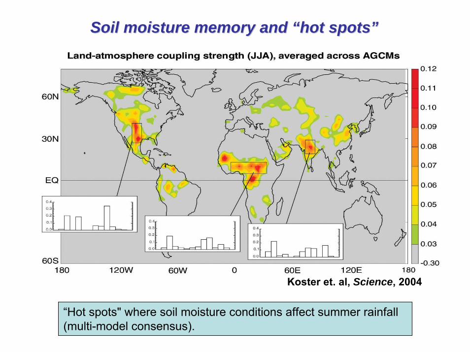
Soil moisture memory and “hot spots”Soil moisture memory and “hot spots”
Koster et. al, Science, 2004
“Hot spots" where soil moisture conditions affect summer rainfall(multi-model consensus).
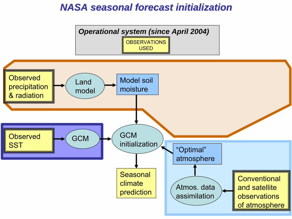
NASA seasonal forecast initializationNASA seasonal forecast initialization
Operational system (since April 2004)OBSERVATIONS
USED
Observed precipitation & radiation
Land model
Model soil moisture
GCM initialization
GCM“Optimal”atmosphere
Atmos. data assimilation
Conventional and satellite observations of atmosphere
Observed SST
Seasonal climate prediction
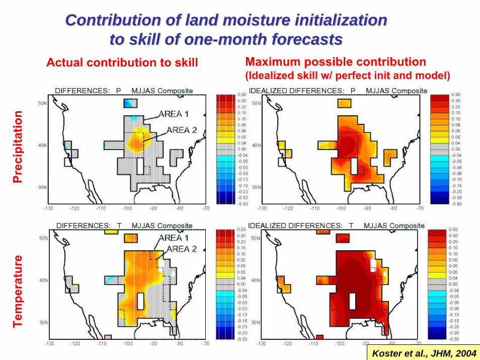
Contribution of land moisture initialization Contribution of land moisture initialization to skill of oneto skill of one--month forecasts month forecasts
Maximum possible contribution (Idealized skill w/ perfect init and model)
Actual contribution to skill
Prec
ipita
tion
Tem
pera
ture
Koster et al., JHM, 2004
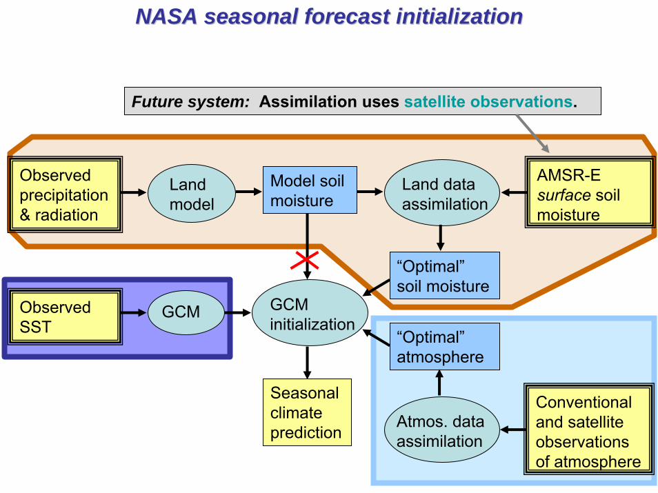
NASA seasonal forecast initializationNASA seasonal forecast initialization
Future system: Assimilation uses satellite observations.
Land data assimilation
AMSR-E surface soil moisture
Observed precipitation & radiation
Land model
Model soil moisture
GCM initialization
Seasonal climate prediction
Observed SST
GCM
“Optimal”soil moisture
“Optimal”atmosphere
Atmos. data assimilation
Conventional and satellite observations of atmosphere
OutlineOutline
Motivation Seasonal climate predictability associated with land surface conditions
Method Land data assimilation with the Ensemble Kalman filter
Soil moisture Satellite observations, uncertainties & data assimilation
Land surface temperature Satellite observations, uncertainties & data assimilation
Conclusions
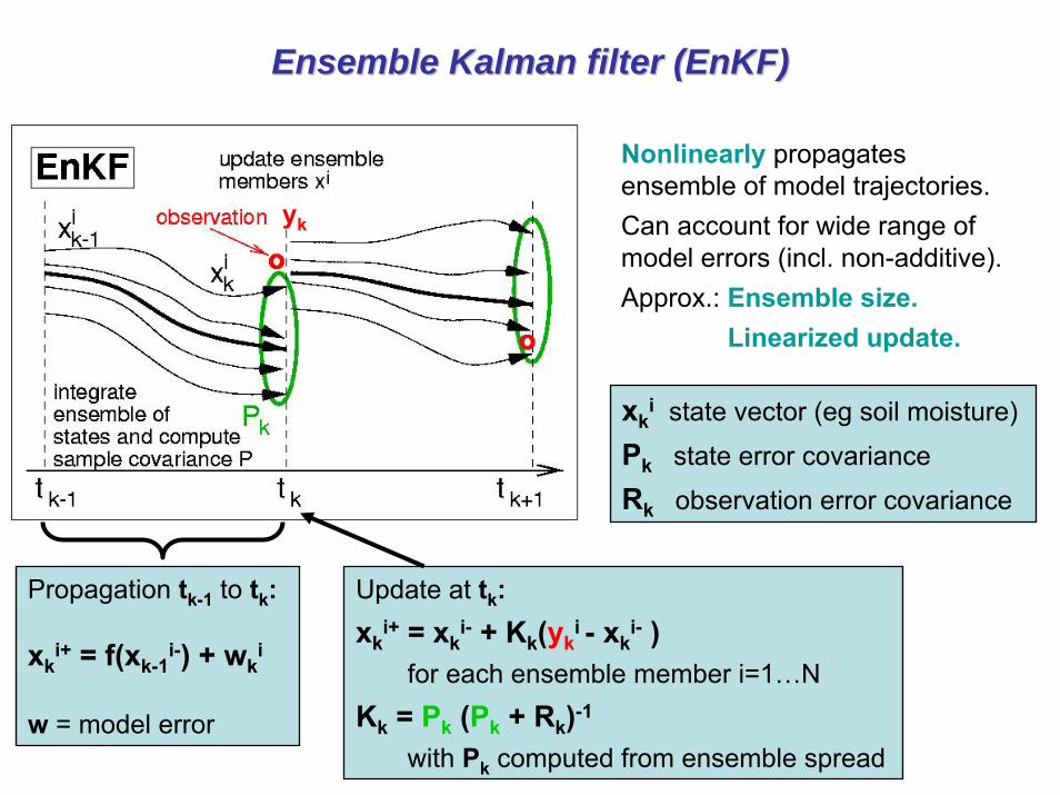
Ensemble Kalman filter (EnKF)Ensemble Kalman filter (EnKF)
yk
Nonlinearly propagates ensemble of model trajectories. Can account for wide range of model errors (incl. non-additive).Approx.: Ensemble size.
Linearized update.
xki state vector (eg soil moisture)
Pk state error covariance
Rk observation error covariance
Propagation tk-1 to tk:
xki+ = f(xk-1
i-) + wki
w = model error
Update at tk:xk
i+ = xki- + Kk(yk
i - xki- )
for each ensemble member i=1…NKk = Pk (Pk + Rk)-1
with Pk computed from ensemble spread
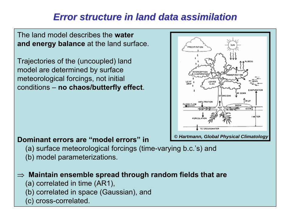
Error structure in land data assimilationError structure in land data assimilation
The land model describes the water and energy balance at the land surface.
Trajectories of the (uncoupled) land model are determined by surface meteorological forcings, not initial conditions – no chaos/butterfly effect.
Dominant errors are “model errors” in (a) surface meteorological forcings (time-varying b.c.’s) and (b) model parameterizations.
⇒ Maintain ensemble spread through random fields that are (a) correlated in time (AR1), (b) correlated in space (Gaussian), and (c) cross-correlated.
© Hartmann, Global Physical Climatology
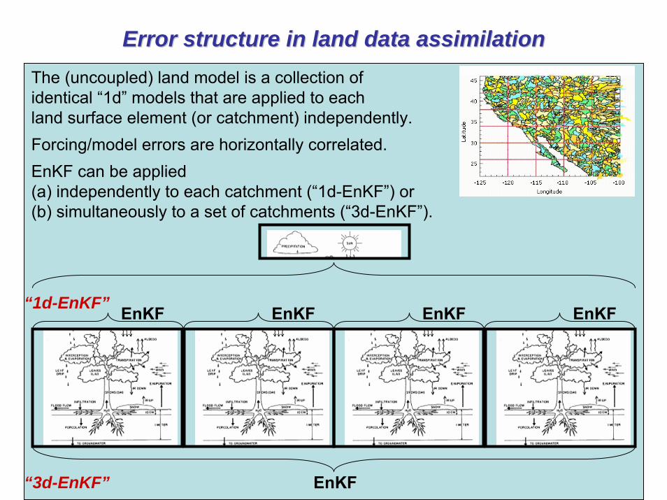
Error structure in land data assimilationError structure in land data assimilationThe (uncoupled) land model is a collection of identical “1d” models that are applied to eachland surface element (or catchment) independently.Forcing/model errors are horizontally correlated.EnKF can be applied (a) independently to each catchment (“1d-EnKF”) or (b) simultaneously to a set of catchments (“3d-EnKF”).
EnKF EnKF EnKF EnKF
“3d-EnKF”
“1d-EnKF”
EnKF
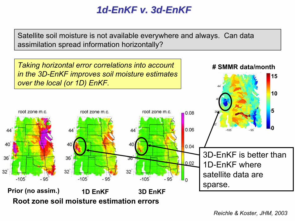
1d1d--EnKF v. 3dEnKF v. 3d--EnKFEnKF
Satellite soil moisture is not available everywhere and always. Can data assimilation spread information horizontally?
1D EnKFPrior (no assim.) 3D EnKF
# SMMR data/month
0
10
5
15
3D-EnKF is better than 1D-EnKF where satellite data are sparse.
Root zone soil moisture estimation errors
Taking horizontal error correlations into account in the 3D-EnKF improves soil moisture estimates over the local (or 1D) EnKF.
Reichle & Koster, JHM, 2003
OutlineOutline
Motivation Seasonal climate predictability associated with land surface conditions
Method Land data assimilation with the Ensemble Kalman filter
Soil moisture Satellite observations, uncertainties & data assimilation
Land surface temperature Satellite observations, uncertainties & data assimilation
Conclusions
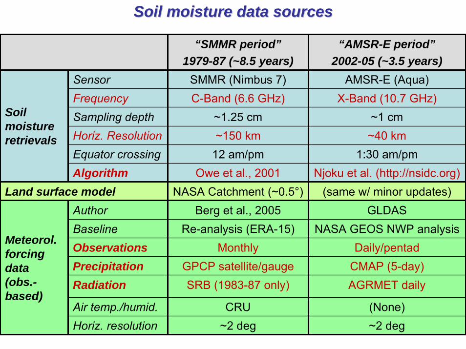
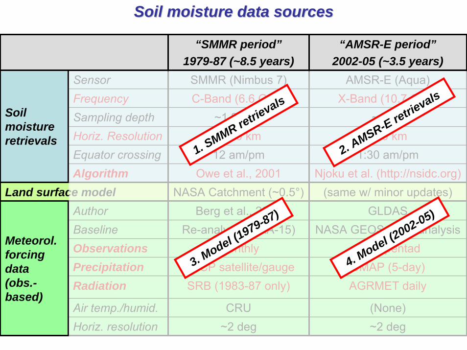
Soil moisture data sourcesSoil moisture data sources
“SMMR period”1979-87 (~8.5 years)
“AMSR-E period”2002-05 (~3.5 years)
Sensor SMMR (Nimbus 7) AMSR-E (Aqua)
Sampling depth ~1.25 cm ~1 cmHoriz. Resolution ~150 km ~40 kmEquator crossing 12 am/pm 1:30 am/pm
Author Berg et al., 2005 GLDASBaseline Re-analysis (ERA-15) NASA GEOS NWP analysis
Air temp./humid. CRU (None)
Observations Monthly Daily/pentadPrecipitation GPCP satellite/gauge CMAP (5-day)Radiation SRB (1983-87 only) AGRMET daily
Algorithm Owe et al., 2001 Njoku et al. (http://nsidc.org)
Soil moisture retrievals
Land surface model
Meteorol. forcing data (obs.-based)
Frequency C-Band (6.6 GHz) X-Band (10.7 GHz)
NASA Catchment (~0.5°) (same w/ minor updates)
Horiz. resolution ~2 deg ~2 deg
1. SMMR retrievals
2. AMSR-E retrievals
3. Model (1
979-87)
4. Model (2
002-05)
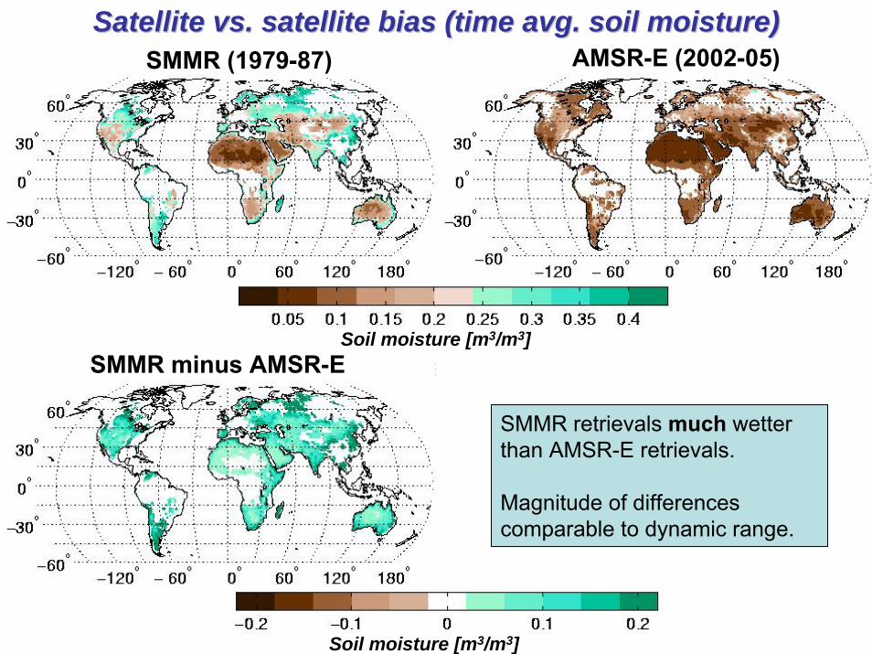
Satellite vs. satellite bias (time avg. soil moisture)Satellite vs. satellite bias (time avg. soil moisture)
SMMR retrievals much wetter than AMSR-E retrievals.
Magnitude of differences comparable to dynamic range.
Soil moisture [m3/m3]
Soil moisture [m3/m3]
SMMR (1979-87)
SMMR minus AMSR-E
AMSR-E (2002-05)
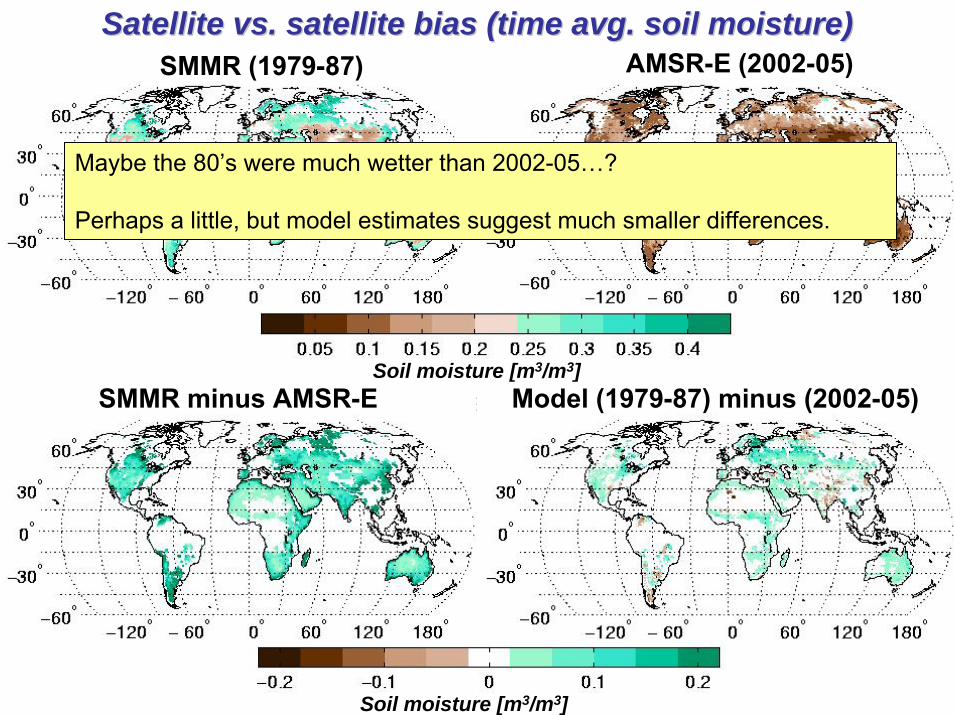
Satellite vs. satellite bias (time avg. soil moisture)Satellite vs. satellite bias (time avg. soil moisture)
Soil moisture [m3/m3]
SMMR (1979-87)
Maybe the 80’s were much wetter than 2002-05…?
Perhaps a little, but model estimates suggest much smaller differences.
SMMR minus AMSR-E Model (1979-87) minus (2002-05)
Soil moisture [m3/m3]
AMSR-E (2002-05)

We found strong biases between AMSR-E and SMMR.
For assimilation, we are really interested in the satellite vs. model biases.
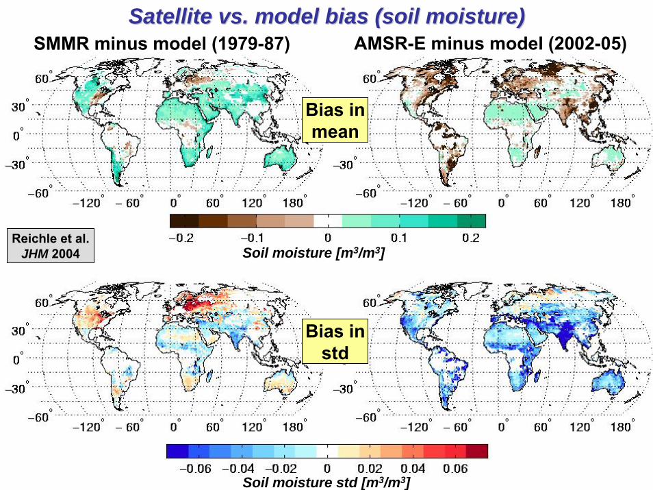
Satellite vs. model bias (soil moisture)Satellite vs. model bias (soil moisture)SMMR minus model (1979-87) AMSR-E minus model (2002-05)
Reichle et al.JHM 2004 Soil moisture [m3/m3]
Bias in mean
Bias in std
Soil moisture std [m3/m3]
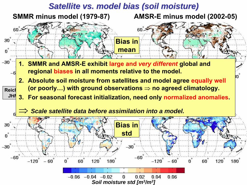
Satellite vs. model bias (soil moisture)Satellite vs. model bias (soil moisture)SMMR minus model (1979-87) AMSR-E minus model (2002-05)
Reichle et al.JHM 2004 Soil moisture [m3/m3]
Bias in mean
Bias in std
1. SMMR and AMSR-E exhibit large and very different global and regional biases in all moments relative to the model.
2. Absolute soil moisture from satellites and model agree equally well(or poorly…) with ground observations ⇒ no agreed climatology.
3. For seasonal forecast initialization, need only normalized anomalies.
⇒ Scale satellite data before assimilation into a model.
Soil moisture std [m3/m3]
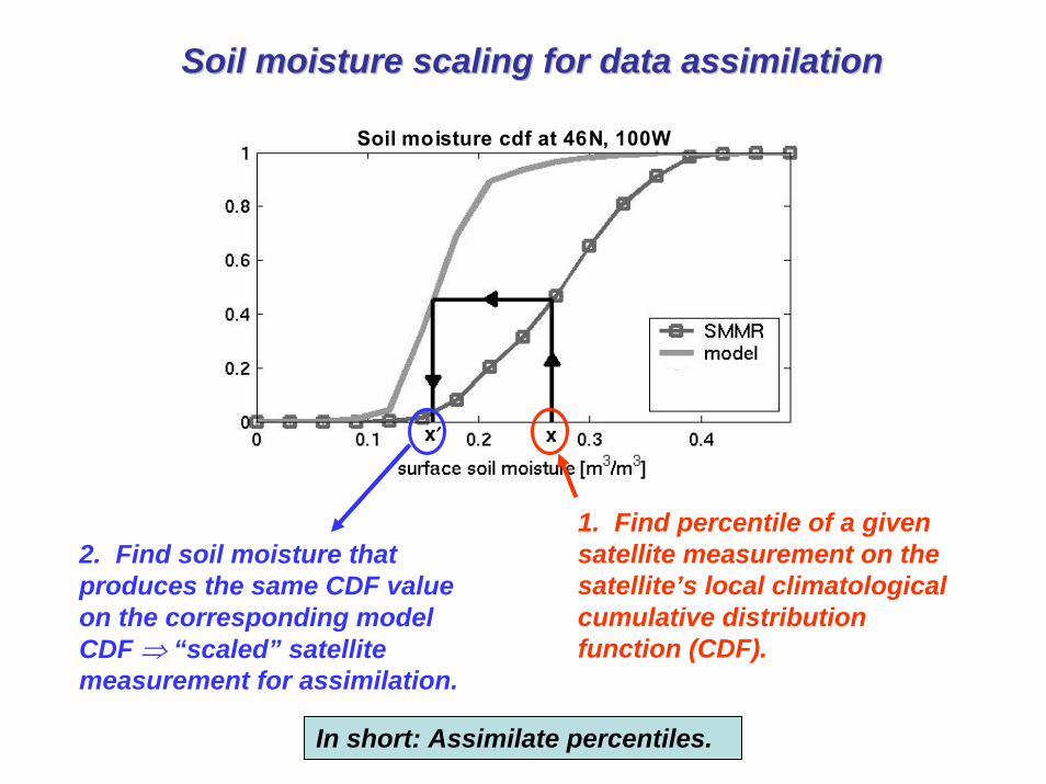
Soil moisture scaling for data assimilationSoil moisture scaling for data assimilation
Soil moisture cdf at 46N, 100W
1. Find percentile of a given satellite measurement on the satellite’s local climatologicalcumulative distribution function (CDF).
2. Find soil moisture that produces the same CDF value on the corresponding model CDF ⇒ “scaled” satellite measurement for assimilation.
In short: Assimilate percentiles.
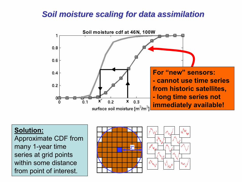
Soil moisture scaling for data assimilationSoil moisture scaling for data assimilation
Soil moisture cdf at 46N, 100W
For “new” sensors:- cannot use time series from historic satellites, - long time series not immediately available!
Solution:Approximate CDF from many 1-year time series at grid points within some distance from point of interest.
2º
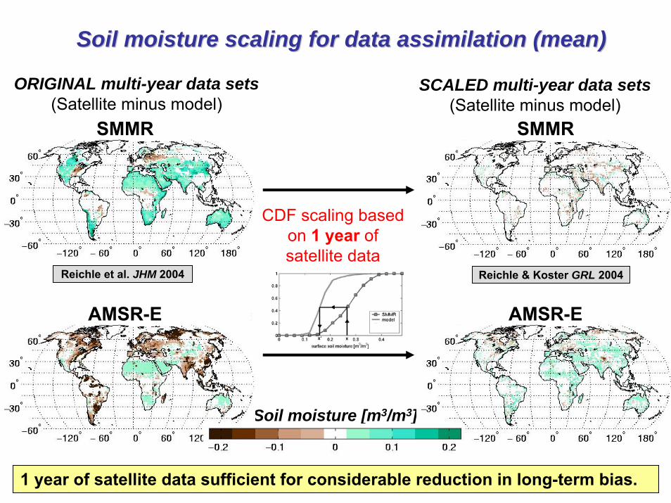
Soil moisture scaling for data assimilation (mean)Soil moisture scaling for data assimilation (mean)
Soil moisture [m3/m3]
ORIGINAL multi-year data sets(Satellite minus model)
SCALED multi-year data sets (Satellite minus model)
CDF scaling based on 1 year of satellite data
AMSR-E
SMMR
AMSR-E
SMMR
Reichle & Koster GRL 2004Reichle et al. JHM 2004
1 year of satellite data sufficient for considerable reduction in long-term bias.
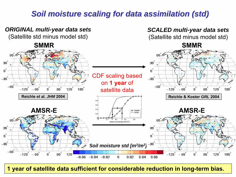
Soil moisture scaling for data assimilation (std)Soil moisture scaling for data assimilation (std)
Soil moisture std [m3/m3]
ORIGINAL multi-year data sets(Satellite std minus model std)
SCALED multi-year data sets (Satellite std minus model std)
CDF scaling based on 1 year of satellite data
AMSR-E
SMMR
AMSR-E
SMMR
Reichle & Koster GRL 2004Reichle et al. JHM 2004
1 year of satellite data sufficient for considerable reduction in long-term bias.

Assimilation of SMMR soil moisture Assimilation of SMMR soil moisture
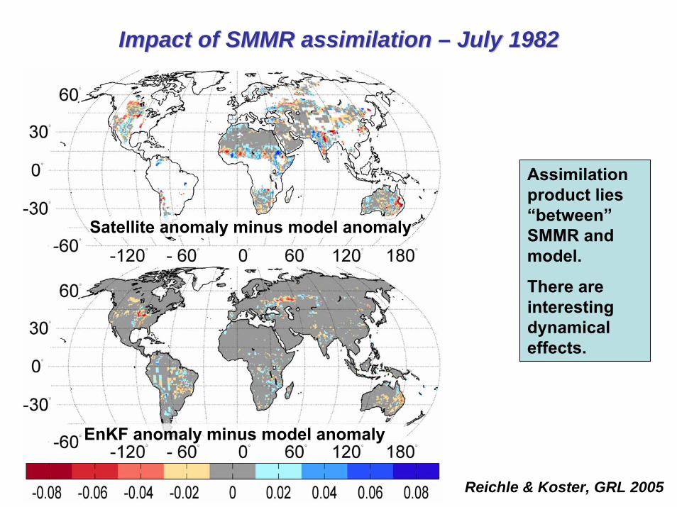
Impact of SMMR assimilation Impact of SMMR assimilation –– July 1982July 1982
Assimilation product lies “between” SMMR and model.
There are interesting dynamical effects.
Satellite anomaly minus model anomaly
EnKF anomaly minus model anomaly
Reichle & Koster, GRL 2005
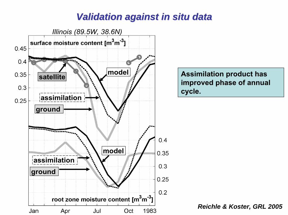
Validation against in situ dataValidation against in situ dataIllinois (89.5W, 38.6N)
modelsatellite
groundassimilation
assimilationground
model
Assimilation product has improved phase of annual cycle.
Reichle & Koster, GRL 2005
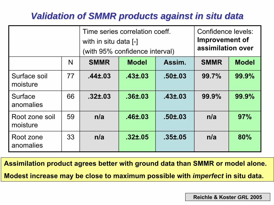
Validation of SMMR products against in situ dataValidation of SMMR products against in situ dataTime series correlation coeff. with in situ data [-] (with 95% confidence interval)
Confidence levels: Improvement of assimilation over
N SMMR Model Assim. SMMR Model
Surface soil moisture
77 .44±.03 .43±.03 .50±.03 99.7% 99.9%
Surface anomalies
66 .32±.03 .36±.03 .43±.03 99.9% 99.9%
Root zone soil moisture
59 n/a .46±.03 .50±.03 n/a 97%
Root zone anomalies
33 n/a .32±.05 .35±.05 n/a 80%
Assimilation product agrees better with ground data than SMMR or model alone.
Modest increase may be close to maximum possible with imperfect in situ data.
Reichle & Koster GRL 2005
Assimilation of SMMR soil moisture Assimilation of SMMR soil moisture
SMMR assimilation successful, but…
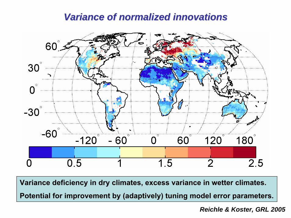
Variance of normalized innovationsVariance of normalized innovations
Variance deficiency in dry climates, excess variance in wetter climates.
Potential for improvement by (adaptively) tuning model error parameters.
Reichle & Koster, GRL 2005

Validation of SMMR products against in situ dataValidation of SMMR products against in situ data
Assimilation product agrees better with ground data than SMMR or model alone.
Modest increase may be close to maximum possible with imperfect in situ data.
Time series correlation coeff. with in situ data [-] (with 95% confidence interval)
Confidence levels: Improvement of assimilation over
N SMMR Model Assim. SMMR Model
Surface soil moisture
77 .44±.03 .43±.03 .50±.03 99.7% 99.9%
Surface anomalies
66 .32±.03 .36±.03 .43±.03 99.9% 99.9%
Root zone soil moisture
59 n/a .46±.03 .50±.03 n/a 97%
Root zone anomalies
33 n/a .32±.05 .35±.05 n/a 80%
We are still working on a similar result for AMSR-E assimilation.
Success is perhaps more difficult to achieve because:
- we have only 3.5 years of AMSR-E (vs. 8.5 years of SMMR),
- AMSR-E retrievals based on X-band (vs. C-band for SMMR),
- GLDAS (2002-05) forcing data (vs. “Berg” 1979-87) might lead to improved (benchmark) model soil moisture.
Reichle & Koster, GRL 2005
Conclusions (soil moisture)Conclusions (soil moisture)
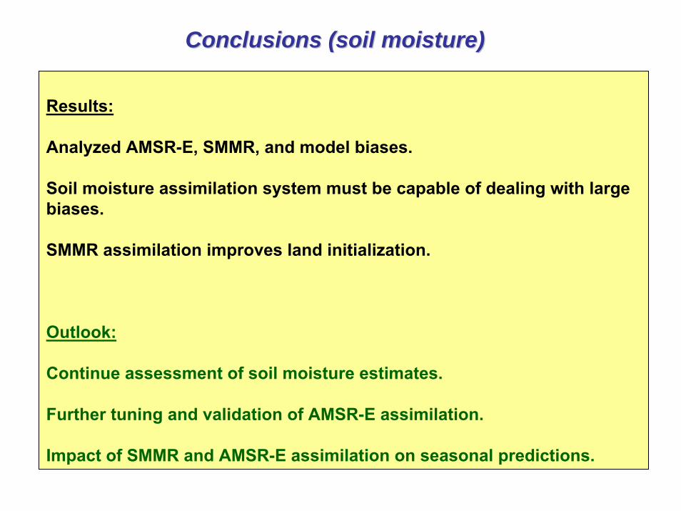
Results:
Analyzed AMSR-E, SMMR, and model biases.
Soil moisture assimilation system must be capable of dealing with large biases.
SMMR assimilation improves land initialization.
Outlook:
Continue assessment of soil moisture estimates.
Further tuning and validation of AMSR-E assimilation.
Impact of SMMR and AMSR-E assimilation on seasonal predictions.
OutlineOutline
Motivation Seasonal climate predictability associated with land surface conditions
Method Land data assimilation with the Ensemble Kalman filter
Soil moisture Satellite observations, uncertainties & data assimilation
Land surface temperature Satellite observations, uncertainties & data assimilation
Conclusions
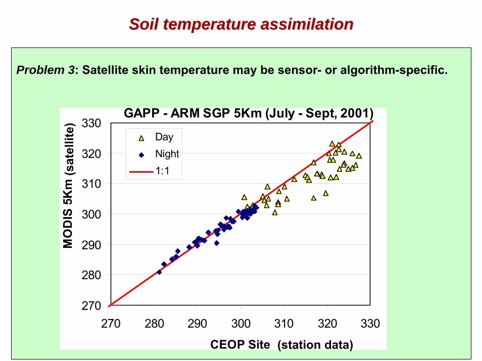
Soil temperature assimilationSoil temperature assimilation
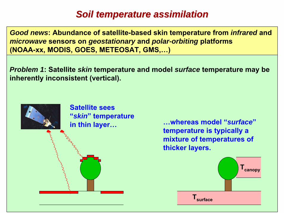
Good news: Abundance of satellite-based skin temperature from infrared and microwave sensors on geostationary and polar-orbiting platforms (NOAA-xx, MODIS, GOES, METEOSAT, GMS,…)
Problem 1: Satellite skin temperature and model surface temperature may be inherently inconsistent (vertical).
…whereas model “surface” temperature is typically a mixture of temperatures of thicker layers.
Satellite sees “skin” temperature in thin layer…
Tsurface
Tcanopy
Soil temperature assimilationSoil temperature assimilation
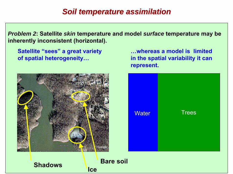
…whereas a model is limited in the spatial variability it can represent.
Satellite “sees” a great variety of spatial heterogeneity…
TreesWater
IceBare soilShadows
Problem 2: Satellite skin temperature and model surface temperature may be inherently inconsistent (horizontal).
Soil temperature assimilationSoil temperature assimilation
GAPP - ARM SGP 5Km (July - Sept, 2001)
270
280
290
300
310
320
330
270 280 290 300 310 320 330
CEOP Site
MO
DIS
5K
m
DayNight1:1
(station data)
(sat
ellit
e)Problem 3: Satellite skin temperature may be sensor- or algorithm-specific.
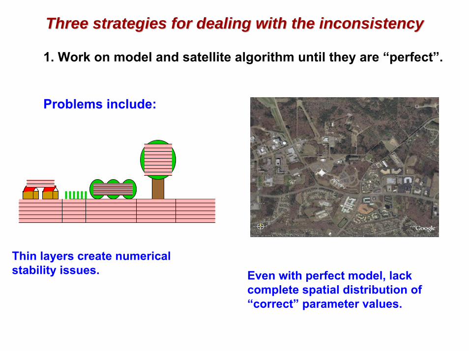
Three strategies for dealing with the inconsistencyThree strategies for dealing with the inconsistency
1. Work on model and satellite algorithm until they are “perfect”.
Problems include:
Thin layers create numerical stability issues. Even with perfect model, lack
complete spatial distribution of “correct” parameter values.
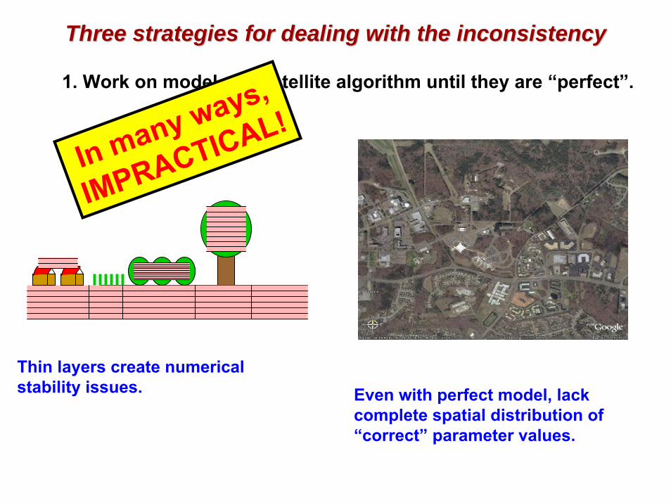
Three strategies for dealing with the inconsistencyThree strategies for dealing with the inconsistency
Problems include:
1. Work on model and satellite algorithm until they are “perfect”.
In many ways,
IMPRACTICAL!
Thin layers create numerical stability issues. Even with perfect model, lack
complete spatial distribution of “correct” parameter values.

Three strategies for dealing with the inconsistencyThree strategies for dealing with the inconsistency
2. Ignore the inconsistencies and hope for the best.

Three strategies for dealing with the inconsistencyThree strategies for dealing with the inconsistency
2. Ignore the inconsistencies and hope for the best.
Questionable results!
(as will be shown)
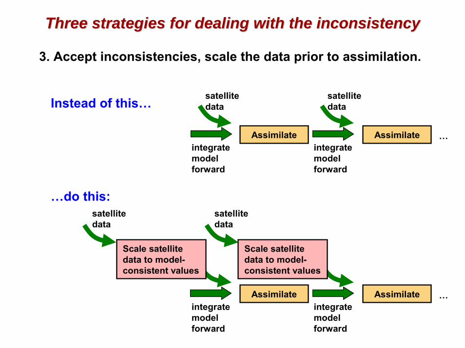
Three strategies for dealing with the inconsistencyThree strategies for dealing with the inconsistency
3. Accept inconsistencies, scale the data prior to assimilation.
integratemodelforward
satellitedata
Assimilateintegratemodelforward
satellitedata
…Assimilate
Instead of this…
…do this:
integratemodelforward
satellitedata
Assimilateintegratemodelforward
satellitedata
…Assimilate
Scale satellite data to model-consistent values
Scale satellite data to model-consistent values

Three strategies for dealing with the inconsistencyThree strategies for dealing with the inconsistency
3. Accept inconsistencies, scale the data prior to assimilation.1) Get time series mean µ and standard deviation σ for satellite Tskin(“T_sat”) and for model-based synthetic Tskin observations (“T_mod”), broken down by diurnal cycle and month.
Jan Feb Mar Apr May Jun Jul Aug Sep Oct Nov Dec
0z µ,σ µ,σ µ,σ µ,σ µ,σ µ,σ µ,σ µ,σ µ,σ µ,σ µ,σ µ,σ
3z µ,σ µ,σ µ,σ µ,σ µ,σ µ,σ µ,σ µ,σ µ,σ µ,σ µ,σ µ,σ
6z µ,σ µ,σ µ,σ µ,σ µ,σ µ,σ µ,σ µ,σ µ,σ µ,σ µ,σ µ,σ
9z µ,σ µ,σ µ,σ µ,σ µ,σ µ,σ µ,σ µ,σ µ,σ µ,σ µ,σ µ,σ
12z µ,σ µ,σ µ,σ µ,σ µ,σ µ,σ µ,σ µ,σ µ,σ µ,σ µ,σ µ,σ
15z µ,σ µ,σ µ,σ µ,σ µ,σ µ,σ µ,σ µ,σ µ,σ µ,σ µ,σ µ,σ
18z µ,σ µ,σ µ,σ µ,σ µ,σ µ,σ µ,σ µ,σ µ,σ µ,σ µ,σ µ,σ
21z µ,σ µ,σ µ,σ µ,σ µ,σ µ,σ µ,σ µ,σ µ,σ µ,σ µ,σ µ,σ
2) Scale satellite Tskin (“T_sat”) into model climatology (std normal deviates):
T_sat_scaled = σ_mod/σ_sat · (T_sat – µ_sat) + µ_mod
3) Assimilate scaled satellite Tskin (“T_sat_scaled”).
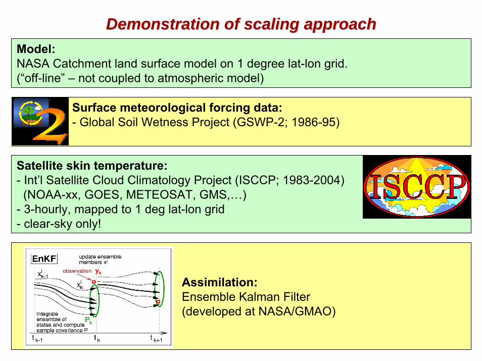
Demonstration of scaling approachDemonstration of scaling approachModel: NASA Catchment land surface model on 1 degree lat-lon grid.(“off-line” – not coupled to atmospheric model)
Surface meteorological forcing data:- Global Soil Wetness Project (GSWP-2; 1986-95)
Satellite skin temperature:- Int’l Satellite Cloud Climatology Project (ISCCP; 1983-2004)(NOAA-xx, GOES, METEOSAT, GMS,…)
- 3-hourly, mapped to 1 deg lat-lon grid- clear-sky only!
Assimilation:Ensemble Kalman Filter(developed at NASA/GMAO)
ykyk

A few DAYS in July 1986 at Ft Peck, MT, USAA few DAYS in July 1986 at Ft Peck, MT, USA
Tskin mean and dynamic range from satellite and model differ. Assimilation w/o scaling increases peak Tskin.
When assimilating w/o scaling, model produces excessive sensible heat flux.
Latent heat flux also increases when soil moisture is available.
Sensible heat flux [W/m2]
Latent heat flux [W/m2]
Tskin [K]
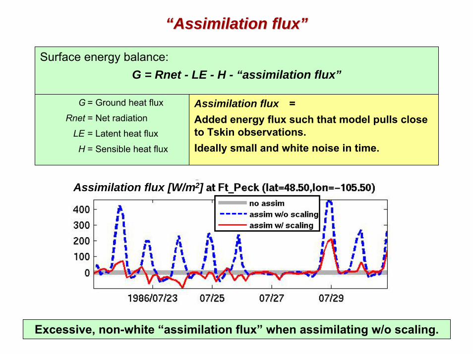
““Assimilation flux”Assimilation flux”
Surface energy balance:G = Rnet - LE - H - “assimilation flux”
G = Ground heat flux
Rnet = Net radiation
LE = Latent heat flux
H = Sensible heat flux
Assimilation flux = Added energy flux such that model pulls close to Tskin observations.Ideally small and white noise in time.
Assimilation flux [W/m2]
Excessive, non-white “assimilation flux” when assimilating w/o scaling.
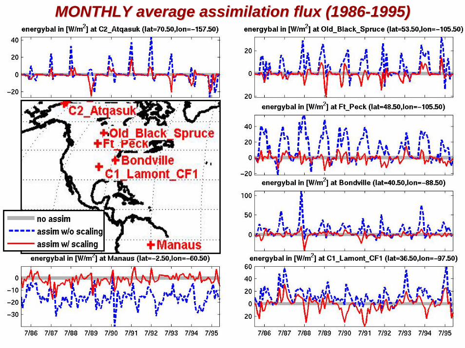
MONTHLY average assimilation flux (1986MONTHLY average assimilation flux (1986--1995)1995)
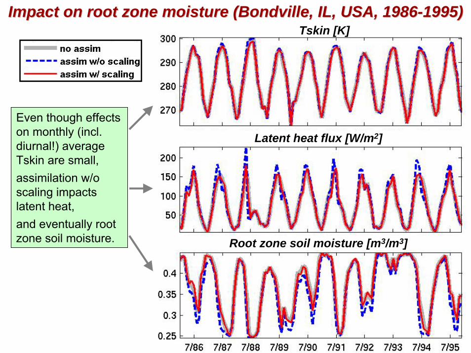
Impact on root zone moisture (Impact on root zone moisture (BondvilleBondville, IL, USA, 1986, IL, USA, 1986--1995)1995)Tskin [K]
Even though effects on monthly (incl. diurnal!) average Tskin are small, assimilation w/o scaling impacts latent heat, and eventually root zone soil moisture.
Latent heat flux [W/m2]
Root zone soil moisture [m3/m3]
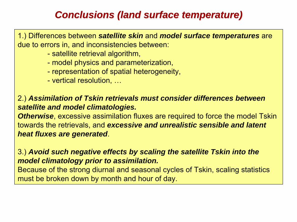
Conclusions (land surface temperature)Conclusions (land surface temperature)
1.) Differences between satellite skin and model surface temperatures are due to errors in, and inconsistencies between:
- satellite retrieval algorithm,- model physics and parameterization,- representation of spatial heterogeneity,- vertical resolution, …
2.) Assimilation of Tskin retrievals must consider differences between satellite and model climatologies.Otherwise, excessive assimilation fluxes are required to force the model Tskintowards the retrievals, and excessive and unrealistic sensible and latent heat fluxes are generated.
3.) Avoid such negative effects by scaling the satellite Tskin into the model climatology prior to assimilation.Because of the strong diurnal and seasonal cycles of Tskin, scaling statistics must be broken down by month and hour of day.
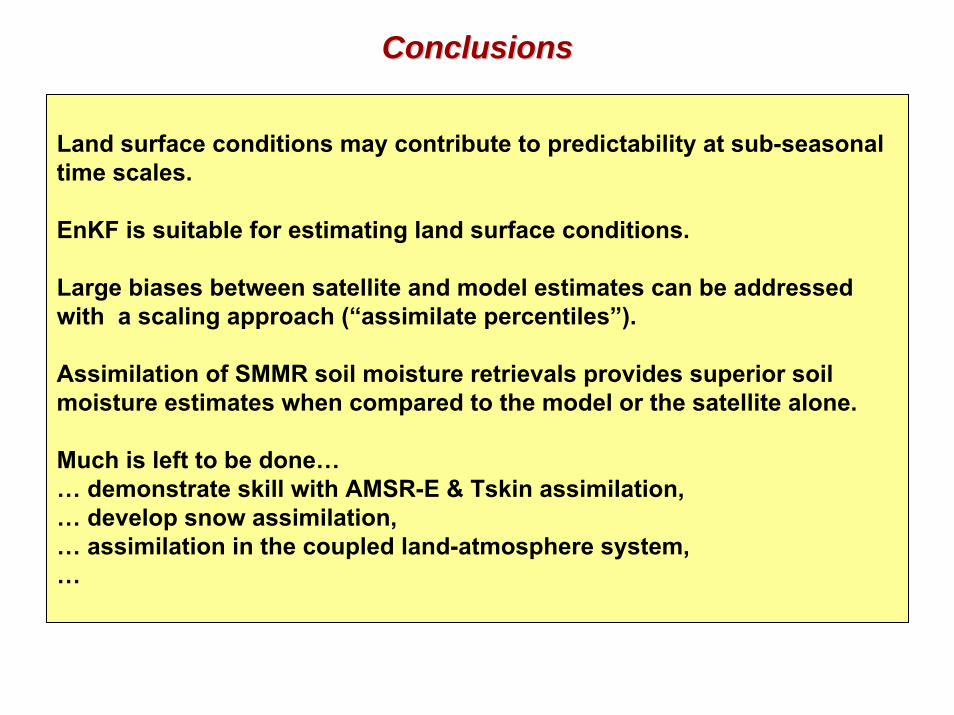
ConclusionsConclusions
Land surface conditions may contribute to predictability at sub-seasonal time scales.
EnKF is suitable for estimating land surface conditions.
Large biases between satellite and model estimates can be addressed with a scaling approach (“assimilate percentiles”).
Assimilation of SMMR soil moisture retrievals provides superior soil moisture estimates when compared to the model or the satellite alone.
Much is left to be done…… demonstrate skill with AMSR-E & Tskin assimilation,… develop snow assimilation,… assimilation in the coupled land-atmosphere system,…

The End