astep south: an antarctic search for transiting exoplanets ... · 2 crouzet et al.: astep south...

HAL Id: hal-00437586https://hal.archives-ouvertes.fr/hal-00437586

Submitted on 14 Dec 2009

HAL is a multi-disciplinary open accessarchive for the deposit and dissemination of sci-entific research documents, whether they are pub-lished or not. The documents may come fromteaching and research institutions in France orabroad, or from public or private research centers.

L’archive ouverte pluridisciplinaire HAL, estdestinée au dépôt et à la diffusion de documentsscientifiques de niveau recherche, publiés ou non,émanant des établissements d’enseignement et derecherche français ou étrangers, des laboratoirespublics ou privés.

ASTEP South: An Antarctic Search for TransitingExoPlanets around the celestial South pole

Nicolas Crouzet, Tristan Guillot, Karim Agabi, Jean-Pierre Rivet, ErickBondoux, Zalpha Challita, Yan Fanteï-Caujolle, François Fressin, Djamel

Mékarnia, François-Xavier Schmider, et al.

To cite this version:Nicolas Crouzet, Tristan Guillot, Karim Agabi, Jean-Pierre Rivet, Erick Bondoux, et al.. ASTEPSouth: An Antarctic Search for Transiting ExoPlanets around the celestial South pole. 2009. <hal-00437586>

https://hal.archives-ouvertes.fr/hal-00437586

https://hal.archives-ouvertes.fr

Astronomy & Astrophysics manuscript no. Crouzet2009.hyper5833 c© ESO 2009December 14, 2009

ASTEP South:

An Antarctic Search for Transiting ExoPlanets

around the celestial South pole

Crouzet N.1, Guillot T.1, Agabi A.2, Rivet J.-P.1, Bondoux E.2,5, Challita Z.2,5, Fanteı-Caujolle Y.2, FressinF.3, Mekarnia D.2, Schmider F.-X.2, Valbousquet F.4, Blazit A.2, Bonhomme S.1, Abe L.2, Daban J.-B.2,

Gouvret C.2, Fruth T.6, Rauer H.6,7, Erikson A.6, Barbieri M.8, Aigrain S.9, Pont F.9

1 Universite de Nice Sophia Antipolis, CNRS UMR 6202, Observatoire de la Cote d’Azur, 06304 Nice Cedex 4, Francee-mail: [email protected]

2 Universite de Nice Sophia Antipolis, CNRS UMR 6525, Observatoire de la Cote d’Azur, 06108 Nice Cedex 2, France3 Harvard-Smithsonian Center for Astrophysics, 60 Garden Street, Cambridge, MA 02138, United States4 Optique et Vision, 6 bis avenue de l’Esterel, BP 69, 06162 Juan-Les-Pins, France5 Concordia Station, Dome C, Antarctica6 DLR Institute for Planetary Research, Rutherfordstrasse 2, 12489 Berlin, Germany7 Center for Astronomy and Astrophysics, TU Berlin, Hardenbergstr. 36, 10623 Berlin, Germany8 Universita di Padova, Dipartimento di Astronomia, vicolo dell’Osservatorio 5, 35122 Padova, Italia9 School of Physics, University of Exeter, Stocker Road, Exeter EX4 4QL, United Kingdom

December 2, 2009

ABSTRACT

Context. The Concordia base in Dome C, Antarctica, is an extremely promising site for photometric astronomy due tothe 3-month long night during the Antarctic winter, favorable weather conditions, and low scintillation.Aims. The ASTEP project (Antarctic Search for Transiting ExoPlanets) is a pilot project to discover transiting planetsand understand the limits of visible photometry from the Concordia site.Methods. ASTEP South is the first phase of the ASTEP project. The instrument is a fixed 10 cm refractor with a 4kx4kCCD camera in a thermalized box, pointing continuously a 3.88 × 3.88◦2 field of view centered on the celestial Southpole. We describe the project and report results of a preliminary data analysis.Results. ASTEP South became fully functional in June 2008 and obtained 1592 hours of data during the 2008 Antarcticwinter. The data are of good quality but the analysis has to account for changes in the PSF (Point Spread Function)due to rapid ground seeing variations and instrumental effects. The pointing direction is stable within 10 arcseconds ona daily timescale and drifts by only 34 arcseconds in 50 days. A truly continuous photometry of bright stars is possiblein June (the noon sky background peaks at a magnitude R ≈ 15 arcsec−2 on June 22), but becomes challenging inJuly (the noon sky background magnitude is R ≈ 12.5 arcsec−2 on July 20). The weather conditions are estimatedfrom the number of stars detected in the field. For the 2008 winter, the statistics are between 56.3 % and 68.4 % ofexcellent weather, 17.9 % to 30 % of veiled weather (when the probable presence of thin clouds implies a lower numberof detected stars) and 13.7 % of bad weather. Using these results in a probabilistic analysis of transit detection, weshow that the detection efficiency of transiting exoplanets in one given field is improved at Dome C compared to atemperate site such as La Silla. For example we estimate that a year-long campaign of 10 cm refractor could reach anefficiency of 69 % at Dome C versus 45 % at La Silla for detecting 2-day period giant planets around target stars frommagnitude 10 to 15. The detection efficiency decreases for planets with longer orbital periods, but in relative sense itis even more favorable to Dome C.Conclusions. This shows the high potential of Dome C for photometry and future planet discoveries.

Key words. Methods: observational, data analysis - Site testing - Techniques: photometric

1. Introduction

Dome C offers exceptional conditions for astronomy thanksto a 3-month continuous night during the Antarctic win-ter and a very dry atmosphere. Dome C is located at75◦06′S − 123◦21′E at an altitude of 3233 meters on a sum-mit of the high Antarctic plateau, 1100 km away from thecoast. After a pioneering summer expedition in 1995, thesite testing for astronomy begun in the early 2000’s. Itrevealed a very clear sky, an exceptional seeing and verylow wind-speeds (Aristidi et al. 2003, 2005; Lawrence et al.

2004; Ashley et al. 2005b; Geissler & Masciadri 2006). TheFrench-Italian base Concordia was constructed at Dome Cfrom 1999 to 2005 to hold various science experiments.Summer time astronomy experiments have been carried out(e.g. Guerri et al. 2007). The study of Dome C for astron-omy during night-time has considerably expanded since thefirst winter-over at Concordia in 2005. The winter site test-ing has shown an excellent seeing above a thin boundarylayer (Agabi et al. 2006; Trinquet et al. 2008; Aristidi et al.2009), a very low scintillation (Kenyon et al. 2006) and ahigh duty cycle (Mosser & Aristidi 2007). Low sky bright-

2 Crouzet et al.: ASTEP South

ness and extinction are also expected (Kenyon & Storey2006).

Time-series observations such as those implied by thedetection of transiting exoplanets should benefit from theseatmospherical conditions and the good phase coverage. Thiscould potentially greatly improve the photometric precisionwhen compared to other temperate sites (Pont & Bouchy2005). A first photometric instrument, PAIX (Chadid et al.2007), was installed at Concordia in December 2006. Alightcurve of the RR Lyrae variable star Sara over 16 nightsin August 2007 is presented in Chadid et al. (2008), andresults of the whole campaign from June to August 2007have been submitted. The sIRAIT instrument also obtainedlightcurves over 10 days on the stars V841 Cen and V1034Cen (Briguglio et al. 2009; Strassmeier et al. 2008).

The ASTEP project (Antarctic Search for TransitingExoPlanets) aims at determining the quality of Dome C asa site for future photometric surveys and to detect tran-siting planets (Fressin et al. 2005). The main instrumentis a 40 cm Newton telescope entirely designed and builtto perform high precision photometry from Dome C. Theobservations will start in winter 2010. A first instrument al-ready on site, ASTEP South, has observed during the 2008and 2009 winters.

We present here the ASTEP South project and resultsfrom the preliminary analysis of the 2008 campaign. Wefirst describe the instrument, the observation strategy andthe field of view. Section 3 discusses the main features ob-tained when running this simple instrument from Dome C:influence of the Sun and the Moon, PSF and pointing vari-ations, as well as temperature effects. In section 4 we detailour duty cycle and infer the weather statistics at Dome Cfor the 2008 winter. These results are combined to a prob-abilistic analysis to infer the potential of ASTEP South forplanet detection and to evaluate Dome C as a site for futureplanet discoveries.

2. Instrumental setup

2.1. The instrument

ASTEP South consists of a 10 cm refractor, a front-illuminated 4096x4096 pixels CCD camera, and a simplemount in a thermalized enclosure. The refractor is a com-mercial TeleVue NP101 and the camera is a ProLines se-ries by Finger Lake Instrumentation equipped with a KAF-16801E CCD by Kodak. For the choice of the camera seeCrouzet et al. (2007). Its quantum efficiency peaks at 63 %at 660 nm and is above 50 % from 550 to 720 nm. Thepixel size is 9 µm and the total CCD size is 3.7 cm. Thepixel response non-uniformity is around 0.5 %. Pixels arecoded on 16 bits, implying a dynamic range of 65535 ADU.The gain is 2 e-/ADU. A filter whose transmission startsat 600 nm is placed before the camera to eliminate bluelight. Given the CCD quantum efficiency, the overall trans-mission (600 to 900nm) is equivalent to that of a large Rband. We use a GM 8 equatorial mount from Losmandy. Athermalized enclosure is used to avoid temperature fluctu-ations. The sides of this enclosure are made with wood andpolystyrene. A double glass window reduces temperaturevariations and its accompanying turbulence on the opticalpath. Windows are fixed together by a teflon part and sep-arated by a 3 mm space filled with nitrogen to avoid vapourmist. The enclosure is thermalized to −20◦C and fans are

used for air circulation. The ASTEP South instrument isshown at Dome C in figure 1.

In order to characterize the quality of Dome C for pho-tometric observations, we have to avoid as much as possibleinstrumental noises and in particular jitter noise, leading toa new observation strategy: the instrument is completelyfixed and points towards the celestial South pole contin-uously. This allows also a low and constant airmass. Theobserved field of view is 3.88 × 3.88◦2, leading to a pixelsize of 3.41 arcsec on the sky. This field contains around8000 stars up to magnitude R = 15. This observation setupleads to stars moving on the CCD from frame to frame andto a widening of the PSF (Point Spread Function) in onedirection, depending on the exposure time.

Test observations were made at the Calern site(Observatoire de la Cote d’Azur) observing the celestialNorth pole, in order to choose the exposure time and thePSF size. A 30 second exposure time and a 2 pixel PSFFWHM (Full Width Half Maximum) lead to only 2 satu-rated stars and a limit magnitude around 14 (from Dome Cthe limit magnitude is increased to 15). An analysis ofthe celestial South pole field from the Guide Star CatalogGSC2.2 with these parameters taking into account the ro-tation of the star during each exposure leads to less than10 % of blended stars. Therefore we adopted these param-eters.

Software programs were developed by our team to con-trol the camera, to run the acquisitions and to transfer andsave the data. The instrument was set up at the Concordiabase in January 2008.

Fig. 1. ASTEP South at Dome C, Antarctica, January2008.

2.2. The South pole field

The distribution of stars in our field of view is shown in fig-ure 2. From the GSC2.2 catalog, we find nearly 8000 starsup to our limit magnitude of 15. We also simulate stellarpopulations in a field of 3.88×3.88◦2 centered on the celes-tial South pole using the Besancon model of the Galaxy1

(Robin et al. 2003) for R-band magnitudes between 10 and18 to calculate the dwarf ratio in the field. The comparisonshows that the Besancon model overestimates the number

1 http://bison.obs-besancon.fr/modele/

Crouzet et al.: ASTEP South 3

Table 1. Number of stars in the 3.88×3.88◦2 celestial Southpole field.

Magnitude 10-11 11-12 12-13 13-14 14-15Total 133 545 1171 2190 3608

R < 2R⊙: 35 243 662 1605 3057R < 1R⊙: 4 50 184 556 1388

R < 0.5R⊙: 0 0 2 9 24

of stars in the field by a factor ∼ 2. However, we believethat the ratio of dwarfs to the total number of stars is, byconstruction of the model, better estimated. The bottompanel of fig. 2 shows that most of the stars brighter thanmagnitude R = 12 are giants (or more accurately largerthan twice our Sun).

Table 1 details the number of stars per magnitude range;the total number of stars is obtained from the GSC2.2 cata-log and the number of dwarfs is estimated using the relativefractions from the Besancon model. From magnitude 10 to15 we have 73.6 % of dwarf stars with radius R < 2R⊙. Thisratio is higher than in other typical fields used in the searchfor transiting planets such as Carina. Based on CoRoTluxsimulations (Fressin et al. 2007), we expect that about oneF, G, K dwarf in 1100 to 1600 should harbor a transitinggiant exoplanet. The South pole field observed by ASTEPSouth is thus, in principle, populated enough for the de-tection of transiting planets (see also Crouzet et al. 2009).We will come back to a realistic estimate of the number ofdetectable exoplanets in section 5.

The advantages of the South pole field are hence ofcourse a continuous airmass, a high ratio of dwarfs to giantstars and a very low contamination by background stars. Onthe other hand, the field is less dense than regions closer tothe galactic plane, so that the actual number of transitingplanets in the field is smaller.

2.3. Temperature conditions

The instrument was set up during the Dome C 2008 summercampaign. The external temperature varied at this timebetween −20 and −30◦C. It was let outside without thermalcontrol until the observations started at the end of April.In winter the external temperature varies between −50 and−80◦C. During the observations, the thermalized box is setto a temperature of −20◦C and the CCD to −35◦C. Becauseof self-heating, the electronics of the camera is around +5◦Cwith some variations (see 3.7).

3. Preliminary data analysis

ASTEP South generates around 60 gigabytes of data perday. Since internet facilities at Dome C are limited to alow stream connection only few hours a day, a whole datatransfer is impossible. Data are stored in external hard disksand repatriated at the end of the winter-over, leading to atleast a 6 month delay between the observations and a fulldata analysis. We thus developed a software program foron-site preliminary data analysis, in order to have a day-to-day feedback of the observations. We detail here the resultsof this preliminary analysis.

Fig. 2. Top panel : Cumulative distribution of the numberof stars in the South pole field as a function of their magni-tude in the R band. The plain line shows results from theBesancon model. The dashed line indicates output from theGSC2.2 catalog. Bottom panel: Ratio of dwarf stars withselected radii (less than 2, 1 and 0.5R⊙, respectively, aslabeled) to the total number of stars in the South pole fieldas a function of R magnitude.

3.1. Preliminary data analysis software program

We developed a software program running on the data atConcordia. For each image of a given day the mean inten-sity is computed. We then process only the 1000 × 1000pixel central part of the frame (0.95×0.95◦2) for faster cal-culations. First, a point source identifier gives the numberof detected stars and their location on the CCD. The 200brightest stars are matched to the GSC 2.2 catalog using ahome-made algorithm, in order to identify the South poleon the CCD. The 30 brightest stars are fitted with a gaus-sian to derive the PSF size. Last, basic aperture photometryis performed for a set of 10 stars without any image calibra-tion. The identification of point sources, the gaussian fit andthe aperture photometry use an IDL version of DAOPHOT(Stetson 1987). A point source is considered as a star if itsflux is 5 times larger then the sky noise. Aperture photom-etry is made with large apertures of diameter 12 and 20pixels, allowing to get all the flux for bright stars. Althoughthese large aperture are not adapted to faint stars, the lowcrowding in our field allows to get reasonable lightcurves.Of course this will be optimized during the complete anal-ysis of data. The camera and CCD temperature are alsorecorded. A small size binary file with these results is senteveryday by email. Plots shown in the following are in UTC


time as recorded by the software program (local time atDome C is UTC +8).

3.2. Magnitude calibration

In order to convert ADU into magnitudes, we perform apreliminary magnitude calibration: we measure the flux ofthe stars on a typical image taken under dark sky and con-vert them into instrumental magnitudes. We then comparethese magnitudes to the ones from the GSC2.2 catalog andobtain the so-called zero point. The image used is a raw im-age, but the local background including bias is subtractedwhen calculating the flux of each stars.

We estimate that the error on these magnitudes shouldbe ±0.3 magnitudes or less. First a comparison of the resultfor all the stars in a given image to that obtained with onlythe stars in the 1000 × 1000 pixel central part yields a 0.2magnitude difference. We estimate that the absence of aflat-field procedure is responsible for that difference andthat its impact on our inferred sky brightness magnitudeshould be smaller. Second, while one may estimate that theGSC2.2 errors on the magnitudes of individual stars can beas large as 0.5, the large number of stars (∼ 7000) impliesthat the mean error should be quite smaller. A 0.3 error onthe inferred magnitudes hence appears to be a conservativeestimate.

In what follows, we will use this ADU to magnitude con-version only for the noon and full-moon sky brightness, notfor the dark sky. This is because our preliminary analysisis based on data processed on the fly in Concordia whichhave not been de-biased. Variations in the bias level are ofthe order of 40 ADU. Given that uncertainty, we estimatethat any measurement of magnitudes larger than 18 mayhave a bias error larger than 0.3 magnitudes and thereforerefrain from mentioning those.

A refined analysis of the full ASTEP South data withall available data is under way and will include an accuratede-biasing and magnitude calibration.

3.3. Influence of the Sun

We first consider the influence of the Sun on the photome-try. It is important to notice that although the Sun disap-pears below the horizon from May 4 to August 9, the skybackground is always higher each day in the period aroundnoon which is therefore less favorable for accurate photo-metric measurements. The minimum altitude of the Sun atnoon occurs on June 21 and is 8.5◦ below the horizon. Theheight and width of the peak of intensity are the small-est around the winter solstice and increase before and afterthis date (figure 3). The increase is not linear but variesfrom one day to another, as also observed with the sIR-AIT instrument (Strassmeier et al. 2008). We attempted tocheck whether this may be due to high altitude clouds butno correlation was found between the sky brightness andthe quality of the night derived by studying the number ofdetected stars (see section 4).

Figure 4 shows variations of the mean intensity as afunction of time for 3 clear days: June 22, July 20 andAugust 20. On June, 21 the height is typically 1600 ADUand images are affected during 4 to 6 hours. From our cal-ibration this corresponds to a magnitude of 15.3 arcsec−2

in the standard R band. The residual noise calculated from

the actual number of photons received from the sky in anaperture of 20 pixels (corresponding to a radius equal to aFWHM of 2.5 pixels) is 4 × 10−3. For larger apertures thenoise will be smaller. Therefore this effect will have a mod-erate impact on the photometry. In July the height growsto typically 20000 ADU, i.e. magnitude 12.6 arcsec−2, anda noticeable brightness increase lasts for 7 to 9 hours. InAugust, this brightness increase lasts 9 to 12 hours.

Fig. 3. Image intensity for all the winter. The bias level isaround 2480 ADU and the scale is half of the CCD dynam-ics. Peaks around noon will affect the photometry.

Fig. 4. Image intensity during 3 typical days in June, Julyand August. The bias level is around 2480 ADU and thescale is half of the CCD dynamics. Due to the Sun, thesky background increases around noon. The correspondingmagnitude for June 22 is 15.3 mag / arcsec2.

The mean intensity of each image and the number ofdetected stars are plotted against the height of the Sunin figure 5. The fact that the sky intensity drops to anundetectable level when the Sun is below −13◦ appears tobe in line with the result from Moore et al. (2008) thatthe Dome C sky may be darker than other sites. However,this conclusion is at most tentative due to the absence ofa bias removal and dark sky magnitude determination. We


notice that the R-band sky magnitude averaged over allobservations for a Sun altitude of −9◦ is 16.6 arcsec−2, verysimilar to that obtained close to the zenith for Paranal inthe R-band, i.e. 16 to 17 arcsec−2 (Patat et al. 2006, seetheir figure 6).

Fig. 5. Mean intensity of each image and number of starsas a function of the Sun altitude when it is between−15◦ and −5◦. The bias level is around 2480 ADU and theintensity scale is the whole CCD dynamics. Points: individ-ual measurements, blue and red: average during ascendingand descending periods respectively. At 9◦ below the hori-zon the sky brightness is 16.6 mag / arcsec2.

3.4. Influence of the Moon

The influence of the Moon is shown in figure 6. The Moonis full on June 18, July 18, August 16 and September 15.An increased sky background is clearly seen around thesedays, up to 80 ADU in June, 100 ADU in July, 500 ADU inAugust and 70 ADU in September. The full Moon in Juneand July corresponds to a good weather, without clouds,and the increase in intensity is low enough to allow pho-tometric observations. In contrast, during the full Moonof August the weather was very bad with high temperature(up to −30◦C), strong wind at ground level (up to 11 m/s),and a very cloudy sky. The very high background is thusinterpreted as due to the reflection of moonlight by clouds.

A typical increase of 80 ADU during the full Moon leadsto a sky brightness of ≈ 18.1 mag / arcsec2. As discussedin section 3.2, this magnitude estimate may change by afraction of a magnitude with a precise bias subtraction.

Fig. 6. Image intensity. The bias level is around 2480 ADUand the scale is 1 % of the CCD dynamics. The sky back-ground increases during 10 days around the full Moon upto typically 18.1 mag / arcsec2.

3.5. Point Spread Function variations

PSF variations are a crucial issue for photometry. We inves-tigate here the PSF variations in the ASTEP South data.For each image, the 30 brightest stars are fitted with a gaus-sian PSF and their FWHM in both direction is calculatedusing DAOPHOT. The mean of the FWHM across the en-tire image is shown as a function of time in figure 7. Thismean FWHM varies between 1.5 and 3.5 pixels over thewinter.

Two kinds of variations are present. First, PSF vari-ations on a timescale smaller than one day are ob-served. We compare them to independent seeing measure-ments at Dome C provided by three dedicated DifferentialImage Motion Monitors (DIMM), two of them forming aGeneralized Seeing Monitor (GSM) (for a description ofthese instruments see Ziad et al. 2008). In order to con-sider only the PSF variations of period smaller than one daywe subtract to the FWHM the difference between the me-dian FWHM and the median seeing for each day. Figure 8shows that on this day timescale the corrected FWHMand the seeing are clearly correlated: the PSF variationson short timescales are mostly due to seeing variations. Aspreviously discussed, the seeing at the ground level whereASTEP South is placed is rather poor: the median value inwinter at 3 meters high reported by Aristidi et al. (2009) is2.37 arcsec with stability periods of 10 to 30 minutes. Thisexplains the short-term variations of our PSFs.

On a timescale larger than one day the correlation is nottrue anymore. This shows that another cause of PSF varia-tions is present. For this larger timescale, two regimes seemto be present, one with a PSF around 1.5 pixels and anotherwith a PSF around 3.0 pixels. These variations are associ-ated with an asymmetrical deformation of the PSF. This


suggests an instrumental cause of PSF variations such asastigmatism and decollimation. Indeed, temperature inho-mogeneities in the thermal enclosure cause mechanical andoptical deformations. Unfortunately these large timescalevariations prevent us from estimating the seeing at theground level directly from our photometric data.

Fig. 7. Mean values of the size of the stars (FWHM) on theCCD in pixels (top panels) and their asymmetry (bottompanels) as a function of the observing day for the months ofJune (top left), July (top right), August (bottom left) andSeptember (bottom right). In the top panels, the blue andgreen curves correspond to the values of the FWHM in thex and y directions, respectively. The mean FWHM valuesare obtained through a spatial average on the CCD.

Fig. 8. Correlation between the PSF FWHM and inde-pendent seeing measurements at Dome C, for timescalessmaller than one day (the FWHM is corrected for largertimescale variations). Direct seeing measurements fromthree Differential Image Motion Monitors are shown in blue,green and red. A linear regression gives a slope a = 0.59with a correlation coefficient r = 0.65. The PSFs are clearlyaffected by seeing variations at the ground level.

3.6. Astrometry and pointing variations

Ideally the pointing should remain stable during all thewinter, meaning that the South pole must stay at the sameplace on the CCD. The position of the South pole on theCCD is found on each image using a home-made field-matching algorithm. The precision of this algorithm is typ-ically 0.2 pixels. The results for a typical day and for allthe winter are shown in figure 9.

First we have a variation of this position with a period ofone sidereal day. This is due to an incomplete correction ofastrometric effects. Indeed, the star coordinates from theGSC2.2 catalog were corrected only for the precession ofthe equinox from the J2000 epoch to January 1, 2008. Theremaining error on the star coordinates led to an error of10 pixels (34 arcsec) in the determination of the position ofthe pole. We then corrected the GSC2.2 coordinates fromthe precession of the equinox using the real observationdate, and from the nutation and the aberration of light (orBradley effect). After these astrometric corrections the polestays within 2 or 3 pixels during the day.

Second, the pole is drifting during the winter. The am-plitude is 10 pixels (34 arcsec) in 50 days, from June 12 toJuly 31. From the orientation of the CCD we find that thisdrift is oriented vertically towards the North. This may bedue to mechanical deformations of the instrument, atmo-spheric changes or a motion of the ice under the instrument.In any case this effect is very small.

3.7. Camera temperature variations

The CCD is cooled down to −35◦C without any variations.In contrast the electronic part of the camera oscillates be-tween +4 and +8◦C with a one hour period (figure 10).A threshold effect explains these variations: the thermal-ized enclosure is not heated continuously but only when itpasses below a threshold temperature. A direct consequenceis seen on the bias images. The bias level oscillates with thesame period and an amplitude of 10 ADU. The mean inten-sity of science images is affected in the same way. The biaslevel is plotted against the camera temperature in figure 11and shows a hysteresis behavior. For a given temperature,the bias level is lower if the temperature is increasing thanif the temperature is decreasing. The hysteresis amplitudeis around 5 ADU. An explanation can be that the tempera-ture sensor is not exactly on the electronics but is stuck ona camera wall which may be sensitive to temperature vari-ations with a time lag compared to the electronics. It mayalso be due to the electronics and sensor having differentthermal inertia.

4. Duty cycle

A main objective of ASTEP South is to qualify the dutycycle for winter observations at Dome C. The observationcalendar for the whole 2008 campaign is shown in figure 12.April and May were mainly devoted to setting up the in-strument and software programs. Continuous observationsstarted around mid-June. Since then, very few interruptionsoccurred and data were acquired until October. The effectof the Sun and of the Moon has already been discussedin section 3. We present here some technical limitations tothe duty cycle, and quantify the photometric quality of theDome C site for this campaign.


precession*

nutation

Bradley effectBradley effect

E

N

W

S

12/0612/06

24/0624/06 02/0702/07

11/0711/07

17/0717/07

31/0731/07

Fig. 9. Position of the pole on the CCD. Top: 9 images onJuly 11 after various astrometric corrections (blue: approx-imate correction of the precession of the equinox, green: im-proved correction of the precession of the equinox, brown:correction of the nutation, red: correction of the Bradley ef-fect). Bottom: 7 days between June 12 and July 30, showinga drift over the winter (dark blue: June 12, light blue: June24, green: July 2, yellow: July 11, orange: July 17, red: July30).

4.1. Technical issues

Technical issues encountered during this campaign limitedthe duty cycle. We show here typical issues that instru-ments at Dome C have to face with. We believe these canbe mostly overcome with appropriate technical solutions.

– First, the shutter did not close and got damaged at tem-peratures below 0◦C. We had to change the shutter andbuild a special thermalization device to warm it.

– In order to install the camera again after changing theshutter, the thermalized box was opened and suddenlycooled by the ambient air at ∼ −60◦C. As a result,cables not made in teflon broke as well as the cameraUSB connection. These had to be replaced.

– Outside instruments are affected by power cuts lastingfor a few minutes to a few hours. The fraction of timelost for observations is negligible, however next instru-

ments should be equipped with converters to avoid pos-sible damages.

– The instrument is submitted to temperature gradientsinside the thermal enclosure, and to the external tem-perature during power cuts or when opening the box.This leads to mechanical constraints resulting in decol-limation and astigmatism.

4.2. Weather conditions at Dome C

A first experiment to measure the winter clear sky frac-tion at Dome C was made by Ashley et al. (2005a) withICECAM, a CCD camera with a lens of 30◦ field of view.Every 2 hours from February to November 2001, ten im-ages of the sky were taken and averaged. An analysis of allthe images yielded a fraction of 74 % of cloud-free time. Ananalysis by Mosser & Aristidi (2007) for the 2006 winteryielded an estimate of 92 % of clear sky fraction by re-porting several times a day the presence of clouds with thenaked eye. Moore et al. (2008) derive a clear sky fraction of

Fig. 10. Camera temperature, bias level and image inten-sity on July 11. The camera temperature varies between +4and +8◦C with a period of one hour and affects the biaslevel and the image intensity to about 10 ADU.

Fig. 11. Bias level against the camera temperature for July11. The blue points correspond to an increasing tempera-ture and the red points to a decreasing temperature, show-ing a hysteresis behavior.


Fig. 12. ASTEP South observation calendar for the 2008campaign. April and may were mainly dedicated to solvingtechnical problems. Continuous observations started mid-June with very few interruptions until the end of the winter.

79 % for the winter 2006 from the Gattini instrument usingthe number of stars and the extinction across the images. Ina previous work, we derived a clear sky fraction of 74 % forthe 2008 winter from the ASTEP South data, consideringthat the sky is clear if we have more than half of the starsdetected on the best images (Crouzet et al. 2010). Howeverthis result is dependent on this ad hoc criterion. We reeval-uate here this fraction by avoiding such an arbitrary limit.

4.2.1. Method

A new measurement of the clear sky fraction is made withASTEP South using a method sensitive to thin clouds,based on the number of stars detected in the field. In or-der to do so, we need to evaluate the number of stars thatshould be detected on any given image if the weather wasexcellent. Our PSF size varies due to fluctuations of the see-ing and of the instrument itself, and the background levelalso changes due to the presence of the Moon and the Sun.Since these are not directly related to weather, we needto derive how the number of detectable stars changes as afunction of these parameters. (Note that thin clouds shouldaffect the seeing in some way, however a posteriori exami-nation of the data shows that this effect is small comparedto the global attenuation due to clouds).

4.2.2. Identifying point sources with DAOPHOT

The 1000 × 1000 pixel sub-images contain up to 500 starsof varying magnitude. Our automatic procedure for find-ing point sources uses the FIND routine from DAOPHOT.Specifically, in this procedure a star is detected if the centralheight of the PSF is above the local background by a givennumber of standard deviations of that background. Thisthreshold parameter α is chosen by the user. We chooseα = 5.

4.2.3. A model to evaluate the expected number of stars

The full width half maximum ω of our PSFs is typically2.5 pixels. To evaluate whether a star is detected or not wecompare the amplitude A of the PSF to the noise in thecentral pixel. We consider two kind of noises: the photonnoise from the sky background Nsky =

√

Fsky and the read-out noise Nron. The noise in the central pixel is hence N =√

N2sky + N2

ron. In order to obtain A as a function of ω we

consider a gaussian PSF. The amplitude A of a gaussianis A = cF/ω2 with F beeing the total flux under the PSFand c ≈ 0.88. The condition to detect a star A ≥ αN canthus be expressed as F ≥ αNω2/c. The limit magnitude mis therefore:

m = −2.5 log(αNω2/c) + Z (1)

with Z being the photometric calibration constant. We haveNron = 10 electrons and set α = 5 as we do in DAOPHOT,and since the instrument is not calibrated photometricallywe use as ad hoc constant Z = 21.6. As an example, typicalvalues in our data are Fsky = 80 electrons and ω = 2.5pixels. This yields m = 14.9.

To derive the number of stars N∗ expected in a1000× 1000 pixel sub-image from this limit magnitude weuse a typical image taken under excellent weather condi-tions. We calculate the distribution in magnitude of thedetected stars and fit it with a 3rd order polynomial. Formagnitudes larger than 14 the number of stars increasesmore slowly because they are becoming too faint to be alldetected. We therefore extend the fitting function with aconstant slope. The following relation provides our assumednumber of stars as a function of the limit magnitude:

log N∗ =

{

a3m3 + a2m

2 + a1m + a0 if m ≤ 14

log N∗14 + 0.2 (m − 14) if m > 14(2)

where a3 = 0.013, a2 = −0.664, a1 = 11.326,a0 = −61.567 and N∗14 is the number of stars detected form = 14. Equations (1) and (2) thus provide the number ofstars that should be detected for a clear sky given a valueof sky background and FWHM. In order to test the validityof this relation, we compare this to the maximum numberof stars detected in our images for given values of FWHMand sky background. (By choosing the maximum numberof stars, or more precisely the number of stars which is ex-ceeded only 1 % of the time, we ensure that we consideronly images taken under excellent weather conditions). Wefind that both agree with a standard error of 6.6 % and amaximum error of 15 %.


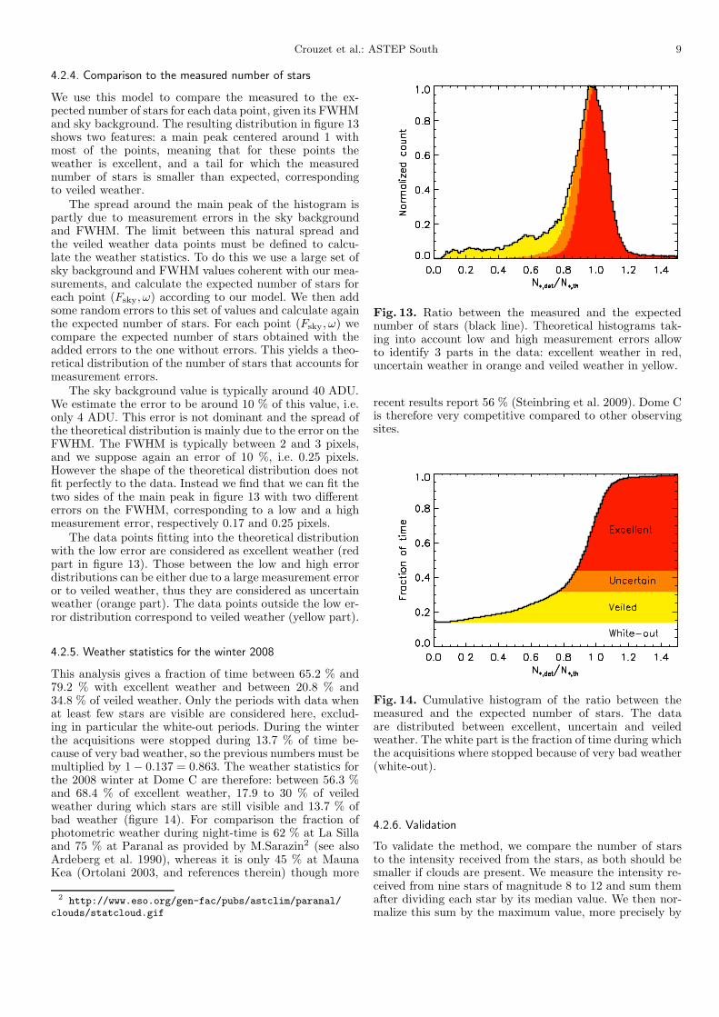
4.2.4. Comparison to the measured number of stars

We use this model to compare the measured to the ex-pected number of stars for each data point, given its FWHMand sky background. The resulting distribution in figure 13shows two features: a main peak centered around 1 withmost of the points, meaning that for these points theweather is excellent, and a tail for which the measurednumber of stars is smaller than expected, correspondingto veiled weather.

The spread around the main peak of the histogram ispartly due to measurement errors in the sky backgroundand FWHM. The limit between this natural spread andthe veiled weather data points must be defined to calcu-late the weather statistics. To do this we use a large set ofsky background and FWHM values coherent with our mea-surements, and calculate the expected number of stars foreach point (Fsky, ω) according to our model. We then addsome random errors to this set of values and calculate againthe expected number of stars. For each point (Fsky, ω) wecompare the expected number of stars obtained with theadded errors to the one without errors. This yields a theo-retical distribution of the number of stars that accounts formeasurement errors.

The sky background value is typically around 40 ADU.We estimate the error to be around 10 % of this value, i.e.only 4 ADU. This error is not dominant and the spread ofthe theoretical distribution is mainly due to the error on theFWHM. The FWHM is typically between 2 and 3 pixels,and we suppose again an error of 10 %, i.e. 0.25 pixels.However the shape of the theoretical distribution does notfit perfectly to the data. Instead we find that we can fit thetwo sides of the main peak in figure 13 with two differenterrors on the FWHM, corresponding to a low and a highmeasurement error, respectively 0.17 and 0.25 pixels.

The data points fitting into the theoretical distributionwith the low error are considered as excellent weather (redpart in figure 13). Those between the low and high errordistributions can be either due to a large measurement erroror to veiled weather, thus they are considered as uncertainweather (orange part). The data points outside the low er-ror distribution correspond to veiled weather (yellow part).

4.2.5. Weather statistics for the winter 2008

This analysis gives a fraction of time between 65.2 % and79.2 % with excellent weather and between 20.8 % and34.8 % of veiled weather. Only the periods with data whenat least few stars are visible are considered here, exclud-ing in particular the white-out periods. During the winterthe acquisitions were stopped during 13.7 % of time be-cause of very bad weather, so the previous numbers must bemultiplied by 1 − 0.137 = 0.863. The weather statistics forthe 2008 winter at Dome C are therefore: between 56.3 %and 68.4 % of excellent weather, 17.9 to 30 % of veiledweather during which stars are still visible and 13.7 % ofbad weather (figure 14). For comparison the fraction ofphotometric weather during night-time is 62 % at La Sillaand 75 % at Paranal as provided by M.Sarazin2 (see alsoArdeberg et al. 1990), whereas it is only 45 % at MaunaKea (Ortolani 2003, and references therein) though more

2 http://www.eso.org/gen-fac/pubs/astclim/paranal/clouds/statcloud.gif

Fig. 13. Ratio between the measured and the expectednumber of stars (black line). Theoretical histograms tak-ing into account low and high measurement errors allowto identify 3 parts in the data: excellent weather in red,uncertain weather in orange and veiled weather in yellow.

recent results report 56 % (Steinbring et al. 2009). Dome Cis therefore very competitive compared to other observingsites.

Fig. 14. Cumulative histogram of the ratio between themeasured and the expected number of stars. The dataare distributed between excellent, uncertain and veiledweather. The white part is the fraction of time during whichthe acquisitions where stopped because of very bad weather(white-out).

4.2.6. Validation

To validate the method, we compare the number of starsto the intensity received from the stars, as both should besmaller if clouds are present. We measure the intensity re-ceived from nine stars of magnitude 8 to 12 and sum themafter dividing each star by its median value. We then nor-malize this sum by the maximum value, more precisely by


the mean of the 1 % highest values. We use only the periodswith a moderate sky background i.e. when the Sun is be-low −13◦ and excluding the full Moon periods (the result ishowever very similar using all data points). Figure 15 showsthe normalized star intensity as a function of the ratio be-tween the measured and the expected number of stars. Asexpected, both parameters are directly correlated, thus val-idating the method. We further note that for data pointstaken under excellent or intermediate weather conditions,i.e. when N∗/N∗th > 0.7, the normalized intensity receivedfrom the stars is 0.77±0.22. Both parameters are thus goodindicators of the cloud cover in the field of view.

Fig. 15. Normalized intensity of a selected sample of ninestars as a function of the ratio between the measured andthe expected number of stars based on theoretical estimates(see text).

4.3. Auroras

Aurorae were first feared to be a source of contaminationfor long-term photometric data. However, it is to be notedthat Concordia is a favorable site in that respect: aurorasoccur mainly in the auroral zone, a ring-shaped region witha radius of approximately 2500 km around the magneticpole. The Concordia site is located well within this ring,only 1300 km from the South magnetic pole, and thus has amuch lower auroral activity than other sites (e.g. Dome A).

During the winter-over 2008, the Concordia staff re-ported 2 auroras on July 30 and 31. On July 30, a carefulexamination of the ASTEP South data indicates a possibil-ity of auroral contamination between 14:12 and 14:24 UTC,but it cannot be distinguished from thin clouds. The July31 data were unfortunately lost during the copy, probablybecause of a hard drive glitch (the only instance of that oc-curring) so that we could not attempt to check the imagesfor that day.

In any case, the ASTEP South 2008 data were not con-taminated by auroras, confirming the low contribution ofauroras to the sky brightness as suggested by Dempseyet al. (2005). It will be interesting to see whether it re-mains true when progressively moving towards a maximumsolar activity in 2012.

4.4. Observing time and photometric quality of Dome C

The duty cycle for the 2008 campaign of ASTEP Southis represented in figure 16. The limit due to the Sun, theobserving time and the excellent and intermediate weatherfractions are shown for each day, as well as the white-out pe-riods. We acquired 1592 hours of data with ASTEP Southon a single field during the 2008 campaign. From the pre-vious analysis we have 1034 hours with excellent or uncer-tain weather. As a comparison, simulations based on themethod described in Rauer et al. (2008) show that the timeusable for photometry in one year at La Silla for the fieldwith the best observability is typically 820 hours per year(see section 5 for more details). Moreover, the white-outperiods at Dome C last typically from one to a few days,allowing extended periods of continuous observations be-tween them. For example we observed every day duringone month between July 9 and August 8. Considering theexcellent and uncertain weather and the hours lost becauseof the Sun, the fraction of time usable for photometry forthis one month period is 52 %. In La Silla the fraction oftime usable for photometry for all one month periods be-tween 1991 and 1999 has a mean of 27 % with a maximumof 45 % in April 1997 (from the La Silla weather statis-tics3 multiplied by the night-time fraction). This shows thevery high potential of Dome C for continuous observationsduring the Antarctic winter.

mar apr may june july aug

ASTEP South @ Concordia, Dome C, 2008

sep

uncertain

veiled

white-outSun altitude <-9°

Sun altitude <-13°

Ob

se

rvin

g t

ime

fra

cti

on

(%

)

excellent

Fig. 16. Daily observing time fraction for ASTEP Southin 2008 as a function of the observation period. The lightblue and dark blue regions indicate the fraction of time forwhich the Sun is lower than −9◦ and −13◦ below the hori-zon, respectively. Periods of excellent, uncertain and veiledweather as observed by ASTEP South are indicated in red,orange and yellow, respectively. White areas correspond toperiods during which observations were not possible, eitherbecause of the Sun altitude or because of bad weather.

5. Planet detection probability

As shown by Pont & Bouchy (2005), the high phase cover-age at Dome C should improve the efficiency of a tran-sit survey. Here we investigate the potential of ASTEP

3 http://www.ls.eso.org/sci/facilities/lasilla/astclim/weather/tablemwr.html


South for transit detection using CoRoTlux and comparethe Dome C and La Silla observing sites. CoRoTlux per-forms statistical simulations of transit events for a surveygiven the star distribution in the field of view, the instru-mental parameters and the observation windows (Fressinet al. 2007, 2009). In all simulations, the star distributionis the one of the South pole field (see section 2.2). We usethe GSC2.2 catalog for stars from magnitude 10 to 14.5completed with a distribution from the Besancon model upto magnitude 18 (after scaling it to the GSC2.2 catalog forlow magnitude stars). The target stars range from magni-tude 10 to 15 and the background stars from magnitude15 to 18. The instrumental parameters are always those ofASTEP South. We perform three simulations correspond-ing to three survey configurations differing only by theirobservation windows.

The first set of observation windows that we haveused in our simulations corresponds to the periods duringwhich ASTEP South actually ran in excellent or uncertainweather conditions in 2008, i.e. the red and orange partsof the duty cycle in figure 16. This provides us with thepotential yield of the 2008 campaign in terms of detectionsof transiting planets.

We also want to compare Dome C and La Silla.In that purpose we consider an ideal campaign for anASTEP South-like instrument for which the observationwindows are determined only from the altitude of the Sunand weather statistics at that site. For Dome C, we applythe weather statistics presented in section 4.2.5 to an entirewinter season in order to generate the second set of obser-vation windows. For this second simulation, we incorporateover the Sun limited duty cycle 13.7 % of white-out periodsand 17.9 % of randomly distributed cloudy periods lastingless than one day.

For La Silla, we generate a third set of observation win-dows using the monthly weather statistics acquired from1987 to 2007 4. The weather statistics for each month istaken as the mean of the photometric fraction for this givenmonth over all years. At La Silla, one cannot simply stareat the South pole field continuously because it is low overthe horizon. A best pointing can be found that maximizesthe observation time as a combination of weather statis-tics, night-time and airmass (for a complete descriptionof the method see Rauer et al. 2008). The resulting fieldwith the best observability is centered on RA= 18h30’ andDE = −58◦54’. For consistency with the other simulationswe use the same stellar population as for the South polefield, and consider that photometric observations are pos-sible when the Sun is less than −9◦ below the horizon. Theresulting duty cycles for weather and Sun limited observa-tions of a single field over one year are shown in figure 17for both Dome C and La Silla. The total observing time istypically 2240 hours for Dome C and 820 hours for La Silla.

A large number of runs (∼ 3000) are performed for eachsurvey configuration in order to have a significant statistic.The results of the simulations provide the number of de-tectable planets. We assume that only transiting planetswith a signal to noise ratio higher than 10 are detectable.This yields 1.08 planets for the ASTEP South 2008 cam-paign (i.e. 3244 planets over 3000 runs), 1.62 planets for awhole winter at Dome C, and 1.04 planet for La Silla. These

4 http://www.eso.org/gen-fac/pubs/astclim/paranal/clouds/statcloud.lis

numbers are low because ASTEP South is a small instru-ment, however the number of planets is notably higher fora survey from Dome C than from La Silla. The resultingplanet detection efficiency is shown in figure 18. The detec-tion efficiency is defined as the number of detectable planetsdivided by the total number of simulated planets. In spiteof technical problems at the beginning of the winter, thedetection efficiency for the ASTEP South 2008 campaignis equivalent to the one obtained for one year at La Silla.When comparing an instrument that would run for the en-tire observing season, the detection efficiency is found tobe significantly higher at Dome C than at La Silla both interms of planet orbital period and transit depth. For exam-ple we have an efficiency of 69 % at Dome C vs 45 % at LaSilla for a 2-day period giant planet, and 76 % at Dome Cvs 45 % at La Silla for a 2 % transit depth. The detectionefficiency decreases for planets with longer orbital periods,but is even more favorable to Dome C relatively to La Silla.On the other hand, it is true that a mid-latitude site offersmore available targets. However, we believe that this showsthe high potential of Dome C for future planet discoveries.

Co

nco

rdia

La SillaLa SillaOb

serv

ing

tim

e f

racti

on

(%

)

jan feb mayaprmar novoctsepaugjuljun dec

Observing period

Fig. 17. Observing time fraction as a function of observ-ing period at Concordia and La Silla. The blue and greyenvelopes indicate values obtained by imposing a Sun al-titude lower than −9◦ below the horizon, for Concordiaand La Silla, respectively. The red histogram is an exam-ple of a generated window function for Concordia using theweather statistics obtained from ASTEP South. The greenhistogram is generated for the field which is observable thelongest with a high-enough airmass at La Silla and usingthe 1987-2007 weather statistics of the site.

6. Conclusion

ASTEP South, the first phase of the ASTEP project ob-served 1592 hours of data. Night-time photometric obser-vations started in a nearly continuous way around mid-June and proceeded to the end of September, when the skybecame too bright even at midnight local-time. Our pre-liminary analysis showed that the Sun affects our photo-metric measurements when it is at an altitude higher than−13◦ below the horizon. The sky brightness at dusk anddawn appears to vary quite significantly from one day tothe other, but its mean is very similar to results obtained


Fig. 18. Calculated efficiency of detection of transiting gi-ant planets for a single field as observed by an ASTEP-South like survey during a full season, and as a functionof the orbital period (top) and transiting depth (bottom).Dotted blue lines: Detection efficiency for the ASTEP South2008 campaign. Plain blue line: Detection efficiency for afull winter at Dome C for a circumpolar field limited onlyby the weather statistics and the constraint of a Sun alti-tude below −9◦. Plain red line: Same as before, but for asurvey at La Silla and the field with the best observabilityover the year (see Fig. 17 and text).

close to the zenith at Paranal (an R-band sky-magnitudeR = 16.6 arcsec−2 for a Sun altitude of −9◦). The full Moonyields a sky brightness of R ≈ 18.1 arcsec−2. Apart from onepossible instance lasting only 12 minutes, auroras had nonoticeable impact on the data.

An identification of the stars in the field allowed us toretrieve the precise location of the celestial South pole onthe images and show that the pointing direction is stablewithin 10 arcseconds on a daily timescale for a drift of only34 arcseconds in 50 days. On the basis of the number ofidentified stars and of a model to account for PSF varia-tions and sky brightness, we retrieved the weather statisticsfor the 2008 winter: between 56.3 % and 68.4 % of excel-lent weather, 17.9 % to 30 % of veiled weather (when theprobable presence of thin clouds implies a lower number ofdetected stars) and 13.7 % of bad weather.

An analysis of the yield of transit surveys with ourweather statistics at Dome C compared to those at La Sillashowed that the efficiency to detect transiting planets inone given field is significantly higher at Dome C (69 %vs. 45 % for 2-day period giant planets with an ASTEPSouth-like instrument in one season). The prospects for thedetection and characterization of exoplanets from Dome Care therefore very good. Future work will be focused on adetailed analysis of the full ASTEP South images. The sec-ond phase of the project includes the installation of ASTEP400, a dedicated automated 40-cm telescope at Concordiaand its operation in 2010.

7. Acknowledgements

The ASTEP project is funded by the Agence Nationale dela Recherche (ANR), the Institut National des Sciences del’Univers (INSU), the Programme National de Planetologie(PNP), and the Plan Pluri-Formation OPERA betweenthe Observatoire de la Cote d’Azur and the Universite deNice-Sophia Antipolis. The entire logistics at Concordia ishandled by the French Institut Paul-Emile Victor (IPEV)and the Italian Programma Nazionale di Ricerche inAntartide (PNRA). The research grant for N. Crouzet issupplied by the Region Provence Alpes Cote d’Azur and theObservatoire de la Cote d’Azur. We wish to further thankE. Fossat for his helpful remarks on the manuscript. Seehttp://fizeau.unice.fr/astep/ for more information aboutthe ASTEP project.

References

Agabi, A., Aristidi, E., Azouit, M., et al. 2006, PASP, 118, 344Ardeberg, A., Lundstrom, I., & Lindgren, H. 1990, A&A, 230, 518Aristidi, E., Agabi, A., Vernin, J., et al. 2003, A&A, 406, L19Aristidi, E., Agabi, K., Azouit, M., et al. 2005, A&A, 430, 739Aristidi, E., Fossat, E., Agabi, A., et al. 2009, A&A, 499, 955Ashley, M. C. B., Burton, M. G., Calisse, P. G., Phillips, A., & Storey,

J. W. V. 2005a, Highlights of Astronomy, 13, 932Ashley, M. C. B., Lawrence, J. S., Storey, J. W. V., & Tokovinin,

A. 2005b, in EAS Publications Series, Vol. 14, EAS PublicationsSeries, ed. M. Giard, F. Casoli, & F. Paletou, 19–24

Briguglio, R., Tosti, G., Strassmeier, K. G., et al. 2009, Memorie dellaSocieta Astronomica Italiana, 80, 147

Chadid, M., Vernin, J., Jeanneaux, F., Mekarnia, D., & Trinquet,H. 2008, in Society of Photo-Optical Instrumentation Engineers(SPIE) Conference Series, Vol. 7012, Society of Photo-OpticalInstrumentation Engineers (SPIE) Conference Series

Chadid, M., Vernin, J., Trinquet, H., et al. 2007, in EAS PublicationsSeries, Vol. 25, EAS Publications Series, ed. N. Epchtein &M. Candidi, 73–75

Crouzet, N., Agabi, K., Blazit, A., et al. 2009, in IAU Symposium,Vol. 253, IAU Symposium, 336–339

Crouzet, N., Guillot, T., Agabi, K., et al. 2010, in EAS PublicationsSeries, EDP, Vol. 40, EAS Publications Series, ed. L. Spinoglio &N. Epchtein, 367–373

Crouzet, N., Guillot, T., Fressin, F., Blazit, A., & the ASTEP team.2007, Astronomische Nachrichten, 328, 805

Dempsey, J. T., Storey, J. W. V., & Phillips, A. 2005, Publicationsof the Astronomical Society of Australia, 22, 91

Fressin, F., Guillot, T., Bouchy, F., et al. 2005, in EAS PublicationsSeries, Vol. 14, EAS Publications Series, ed. M. Giard, F. Casoli,& F. Paletou, 309–312

Fressin, F., Guillot, T., Morello, V., & Pont, F. 2007, A&A, 475, 729Fressin, F., Guillot, T., & Nesta, L. 2009, A&A, 504, 605Geissler, K. & Masciadri, E. 2006, in Society of Photo-Optical

Instrumentation Engineers (SPIE) Conference Series, Vol. 6267,Society of Photo-Optical Instrumentation Engineers (SPIE)Conference Series


Guerri, G., Abe, L., Aristidi, E., et al. 2007, in EAS PublicationsSeries, Vol. 25, EAS Publications Series, ed. N. Epchtein &M. Candidi, 339–342

Kenyon, S. L., Lawrence, J. S., Ashley, M. C. B., et al. 2006, PASP,118, 924

Kenyon, S. L. & Storey, J. W. V. 2006, PASP, 118, 489Lawrence, J. S., Ashley, M. C. B., Tokovinin, A., & Travouillon, T.

2004, Nature, 431, 278Moore, A., Allen, G., Aristidi, E., et al. 2008, in Society of Photo-

Optical Instrumentation Engineers (SPIE) Conference Series, Vol.7012, Society of Photo-Optical Instrumentation Engineers (SPIE)Conference Series

Mosser, B. & Aristidi, E. 2007, PASP, 119, 127Ortolani, S. 2003, ESPAS Site Summary Ser. 1.2, Mauna Kea

(Garching: ESO), 2Patat, F., Ugolnikov, O. S., & Postylyakov, O. V. 2006, A&A, 455,

385Pont, F. & Bouchy, F. 2005, in EAS Publications Series, Vol. 14, EAS

Publications Series, ed. M. Giard, F. Casoli, & F. Paletou, 155–160Rauer, H., Fruth, T., & Erikson, A. 2008, PASP, 120, 852Robin, A. C., Reyle, C., Derriere, S., & Picaud, S. 2003, A&A, 409,

523Steinbring, E., Cuillandre, J., & Magnier, E. 2009, PASP, 121, 295Stetson, P. B. 1987, PASP, 99, 191Strassmeier, K. G., Briguglio, R., Granzer, T., et al. 2008, A&A, 490,

287Trinquet, H., Agabi, A., Vernin, J., et al. 2008, PASP, 120, 203Ziad, A., Aristidi, E., Agabi, A., et al. 2008, A&A, 491, 917

astep south: an antarctic search for transiting exoplanets ... · 2 crouzet et al.: astep south...

Documents