astron. astrophys. 334, 409–419 (1998) astronomy and...

Astron. Astrophys. 334, 409–419 (1998) ASTRONOMYAND

ASTROPHYSICS

Moving gravitational lenses:imprints on the cosmic microwave background

N. Aghanim1, S. Prunet1, O. Forni1, and F.R. Bouchet2

1 IAS-CNRS, Universite Paris XI, Batiment 121, F-91405 Orsay Cedex, France2 IAP-CNRS, 98 bis, Boulevard Arago, F-75014 Paris, France

Received 4 December 1997 / Accepted 2 March 1998

Abstract. With the new generation of instruments for CosmicMicrowave Background (CMB) observations aiming at an ac-curacy level of a few percent in the measurement of the angularpower spectrum of the anisotropies, the study of the contribu-tions due to secondary effects has gained impetus. Furthermore,a reinvestigation of the main secondary effects is crucial in orderto predict and quantify their effects on the CMB and the errorsthat they induce in the measurements.

In this paper, we investigate the contribution, to the CMB,of secondary anisotropies induced by the transverse motions ofclusters of galaxies. This effect is similar to the Kaiser-Stebbinseffect. In order to address this problem, we model the gravita-tional potential well of an individual structure using the Navarro,Frenk & White profile. We generalise the effect of one structureto a population of objects predicted using the Press-Schechterformalism. We simulate maps of these secondary fluctuations,compute the angular power spectrum and derive the averagecontributions for three cosmological models. We then investi-gate a simple method to separate this new contribution from theprimary anisotropies and from the main secondary effect, theSunyaev-Zel’dovich kinetic effect from the lensing clusters.

Key words: galaxies: clusters: general – cosmic microwavebackground – gravitational lensing

1. Introduction

During the next decade, several experiments are planned to ob-serve the Cosmic Microwave Background (CMB) and measureits temperature fluctuations (Planck surveyor, Map, Boomerangetc.). Their challenge is to measure the small scales anisotropiesof the CMB (a few arcminutes up to ten degrees scale) with sen-sitivities better by a factor 10 than the COBE satellite (Smoot etal. 1992). These high sensitivity and resolution measurementswill tightly constrain the value of the main cosmological pa-rameters (Kamionkowski et al. 1994). However, the constraintscan only be set if we are able to effectively measure theprimarytemperature fluctuations. These fluctuations, present at recom-bination, give an insight into the early universe since they are

Send offprint requests to: N. Aghanim

directly related to the initial density perturbations which are theprogenitors to the cosmic structures (galaxies and galaxies clus-ters) in the present universe; but which are first and foremostthe relics of the very early initial conditions of the universe.

Between recombination and the present time, the CMB pho-tons could have undergone various interactions with the matterand structures present along their lines of sight. Some of these in-teractions can induce additional temperature fluctuations called,secondaryanisotropies because they are generated after the re-combination. Along a line of sight, one measures temperaturefluctuations which are the superposition of theprimary andsec-ondaryanisotropies. As a result, and in the context of the futureCMB experiments, accurate analysis of the data will be neededin order to account for the foreground contributions due to thesecondary fluctuations. Photon-matter interactions between re-combination and the present time are due to the presence ofionised matter or to variations of the gravitational potential wellsalong the lines of sight.

The CMB photons interact with the ionised matter mainlythrough Compton interactions. In fact, after recombination theuniverse could have been re-ionised globally or locally. Globalearly re-ionisation has been widely studied (see Dodelson &Jubas 1995 for a recent review and references therein). Its maineffect is to either smooth or wipe out some of the primaryanisotropies; but the interactions of the photons with the mat-ter in a fully ionised universe can also give rise to secondaryanisotropies through the Vishniac effect (Vishniac 1987). Thissecond order effect has maximum amplitudes for a very earlyre-ionisation. The case of a late inhomogeneous re-ionisationand its imprints on the CMB fluctuations has been investigated(Aghanim et al. 1996) and found to be rather important. Inthis case, the secondary anisotropies are due to the bulk mo-tion of ionised clouds with respect to the CMB frame. Whenthe re-ionisation is localised in hot ionised intra-cluster me-dia the photons interact with the free electrons. The inverseCompton scattering between photons and electrons leads to theso-called Sunyaev-Zel’dovich (hereafter SZ) effect (Sunyaev &Zel’dovich1972, 1980). The Compton distortion due to the mo-tion of the electrons in the gas is called the thermal SZ effect.The kinetic SZ effect is a Doppler distortion due to the pecu-liar bulk motion of the cluster with respect to the Hubble flow.The SZ thermal effect has the unique property of depressing the

410 N. Aghanim et al.: Moving gravitational lenses: imprints on the cosmic microwave background

CMB brightness in the Rayleigh-Jeans region and increasing itsbrightness above a frequency of about 219 GHz. This frequencydependence makes it rather easy to observe and separate fromthe kinetic SZ effect. In fact, the latter has a black body spec-trum which makes the spectral confusion between kinetic SZand primary fluctuations a serious problem. The SZ effect hasbeen widely studied for individual clusters and for populationsof clusters. For full reviews on the subject we refer the reader totwo major articles: Rephaeli 1995 and Birkinshaw 1997. Theseinvestigations have clearly shown that the SZ effect in clusters ofgalaxies provides a powerful tool for cosmology through mea-surements of the Hubble constant, the radial peculiar velocityof clusters and consequently the large scale velocity fields.

Besides the interactions with the ionised matter, some sec-ondary effects arise when the CMB photons traverse a varyinggravitational potential well. In fact, if the gravitational potentialwell crossed by the photons evolves between the time they enterthe well and the time they leave it, the delay between entranceand exit is equivalent to a shift in frequency, which induces atemperature anisotropy on the CMB. This effect was first studiedby Rees & Sciama (1968) for a potential well growing underits own gravity. Numerous authors have investigated the po-tential variations due to collapsing objects and their effect onthe CMB (Kaiser 1982, Nottale 1984, Martinez-Gonzalez, Sanz& Silk 1990, Seljak 1996). Similarly, a gravitational potentialwell moving across the line of sight is equivalent to a varyingpotential and will thus imprint secondary fluctuations on theCMB. This effect was first studied for one cluster of galaxies byBirkinshaw & Gull (1983) (Sect. 2). Kaiser & Stebbins (1984)and Bouchet, Bennett & Stebbins (1988) investigated a similareffect for moving cosmic strings. Recent work (Tuluie & La-guna 1995, Tuluie, Laguna & Anninos 1996) based on N-bodysimulations has pointed out this effect in a study of the effectof varying potential on rather large angular scales (' 1). Adiscussion of some of these results and a comparison with ourswill follow in the next sections.

In this paper, following the formalism of Birkinshaw & Gull(1983) and Birkinshaw (1989), we investigate the contributionof secondary anisotropies due to a population of collapsed ob-jects moving across the line of sight, these objects range fromsmall groups to rich clusters in scale (1013 to 1015 M). InSect. 2., we first study in detail the case of a unique collapsedstructure. We use a structure model to compute in particular thedeflection angle and derive the spatial signature of the movinglens effect. We then account (Sect. 3.) for the contribution, tothe primordial cosmological signal, of the whole population ofcollapsed objects using predicted counts and we simulate mapsof these secondary anisotropies. In Sect. 4., we analyse the sim-ulated maps and present our results. We give our conclusions inSect. 5.

2. Formalism for an individual moving structure

One of the first studies of the photon-gravitational potential wellinteractions is related to the Sachs-Wolfe effect (Sachs & Wolfe1967). At the recombination time (z ' 1100) the photons and

matter decouple while they are in potential wells; the photons areredshifted when they leave the potential wells. This generatesthe large angular scale temperature fluctuations.

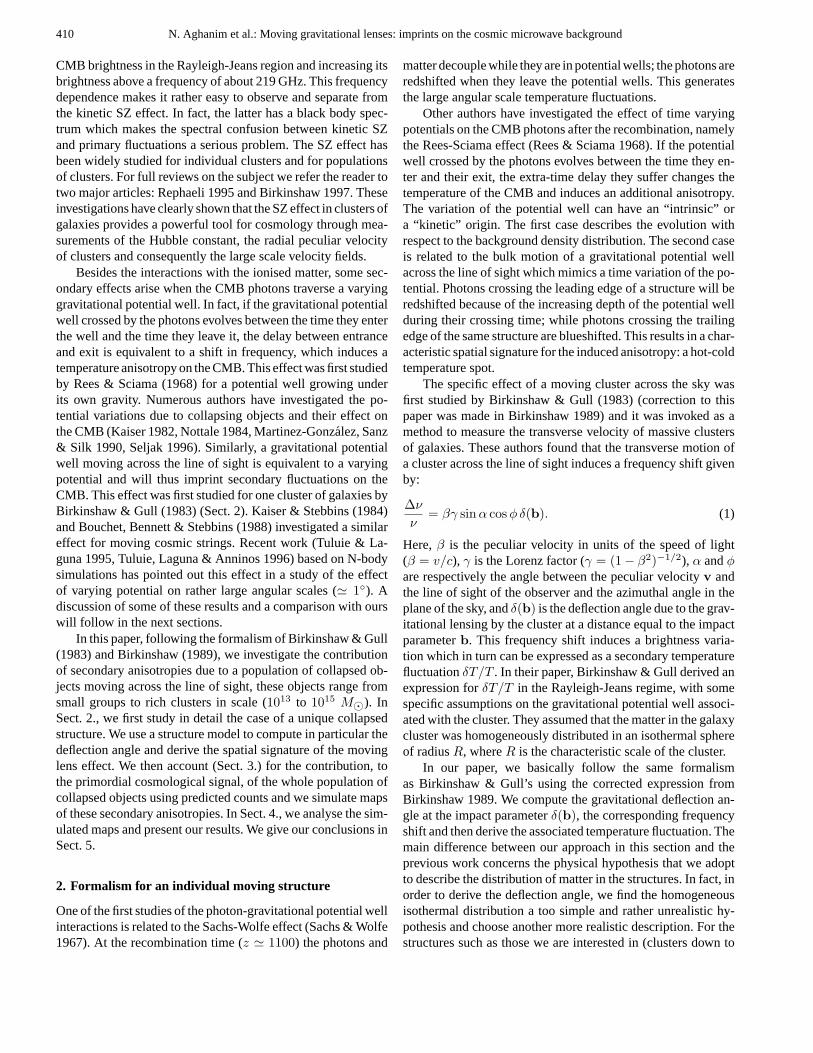
Other authors have investigated the effect of time varyingpotentials on the CMB photons after the recombination, namelythe Rees-Sciama effect (Rees & Sciama 1968). If the potentialwell crossed by the photons evolves between the time they en-ter and their exit, the extra-time delay they suffer changes thetemperature of the CMB and induces an additional anisotropy.The variation of the potential well can have an “intrinsic” ora “kinetic” origin. The first case describes the evolution withrespect to the background density distribution. The second caseis related to the bulk motion of a gravitational potential wellacross the line of sight which mimics a time variation of the po-tential. Photons crossing the leading edge of a structure will beredshifted because of the increasing depth of the potential wellduring their crossing time; while photons crossing the trailingedge of the same structure are blueshifted. This results in a char-acteristic spatial signature for the induced anisotropy: a hot-coldtemperature spot.

The specific effect of a moving cluster across the sky wasfirst studied by Birkinshaw & Gull (1983) (correction to thispaper was made in Birkinshaw 1989) and it was invoked as amethod to measure the transverse velocity of massive clustersof galaxies. These authors found that the transverse motion ofa cluster across the line of sight induces a frequency shift givenby:

∆ν

ν= βγ sinα cos φ δ(b). (1)

Here,β is the peculiar velocity in units of the speed of light(β = v/c), γ is the Lorenz factor (γ = (1 − β2)−1/2), α andφare respectively the angle between the peculiar velocityv andthe line of sight of the observer and the azimuthal angle in theplane of the sky, andδ(b) is the deflection angle due to the grav-itational lensing by the cluster at a distance equal to the impactparameterb. This frequency shift induces a brightness varia-tion which in turn can be expressed as a secondary temperaturefluctuationδT/T . In their paper, Birkinshaw & Gull derived anexpression forδT/T in the Rayleigh-Jeans regime, with somespecific assumptions on the gravitational potential well associ-ated with the cluster. They assumed that the matter in the galaxycluster was homogeneously distributed in an isothermal sphereof radiusR, whereR is the characteristic scale of the cluster.

In our paper, we basically follow the same formalismas Birkinshaw & Gull’s using the corrected expression fromBirkinshaw 1989. We compute the gravitational deflection an-gle at the impact parameterδ(b), the corresponding frequencyshift and then derive the associated temperature fluctuation. Themain difference between our approach in this section and theprevious work concerns the physical hypothesis that we adoptto describe the distribution of matter in the structures. In fact, inorder to derive the deflection angle, we find the homogeneousisothermal distribution a too simple and rather unrealistic hy-pothesis and choose another more realistic description. For thestructures such as those we are interested in (clusters down to

N. Aghanim et al.: Moving gravitational lenses: imprints on the cosmic microwave background 411

Fig. 1. Characteristic spatial signature of atemperature fluctuation due to a moving lenswith massM = 1015 M and velocityv =600 km/s.

small groups), almost all the mass is “made” of dark matter.In order to study the gravitational lensing of a structure prop-erly, one has to model the gravitational potential well using thebest possible knowledge for the dark matter distribution. Thecorrections, due to the more accurate profile distribution thatwe introduce, will not alter the maximum amplitude of an indi-vidual moving lens effect since it is associated with the centralpart of the lens. However, when dealing with some average sig-nal coming from these secondary anisotropies, the contributionfrom the outskirts of the structures appears important and thusa detailed model of the matter profile is needed.

In view of the numerous recent studies on the formation ofdark matter halos, which are the formation sites for the individ-ual structures such as clusters of galaxies, we now have a ratherprecise idea of their formation and density profiles. Specifi-cally, the results of Navarro, Frenk & White (1996, 1997) areparticularly important. In fact, these authors have used N-bodysimulations to investigate the structure of dark matter halos inhierarchical cosmogonies; their results put stringent constraintson the dark matter profiles. Over about four orders of magni-tudes in mass (ranging from the masses of dwarf galaxy halosto those of rich clusters of galaxies), they found that the densityprofiles can be fitted over two decades in radius by a “univer-sal” law (hereafter NFW profile) which seems to be the bestdescription of the structure of dark matter halos (Huss, Jain &Steinmetz 1997). The NFW profile is given by:

ρ(r) =ρcrit δc

(r/rs)(1 + r/rs)2, (2)

wherers = r200/c is the scale radius of the halo,δc its charac-teristic overdensity,ρcrit is the critical density of the universeandc is a dimensionless parameter called the concentration. Theradiusr200 is the radius of the sphere where the mean densityis 200 × ρcrit. This is what we refer to as a virialised object ofmassM200 = 200ρcrit (4π/3)r3

200.

In addition to the fact that the shape is independent of thehalo mass over a wide range, the NFW profile is also inde-pendent of the cosmological model. The cosmological modelintervenes essentially in the formation epoch of the dark matterhalo and therefore in the parameters of the profile, namelyc, rs

andδc.Using the density profile, one can compute the deflection

angle at the impact parameter which gives the shape of the pat-tern and the amplitude of the induced secondary anisotropy. Inour work, we compute the deflection angle following the for-malism of Blandford & Kochanek (1987), which is given by theexpression:

δ = 2Dls

Dos∇r

∫Φ(r, l) dl, (3)

here, the integral is performed over the length elementdl alongthe line of sight.Dls andDos are respectively the distances be-tween lens and source and the observer and source. In the red-shift range of the considered structures (z < 1.5), the distanceratiosDls/Dos range between 1 and 0.68 for the standard CDMmodel, between 1 and 0.53 for the open CDM and between 1 and0.74 for the lambda CDM model. These cosmological modelswill be defined in the next section. In Eq. 3r is the position ofthe structure andΦ(r, l) is the associated gravitational potential.In order to get an analytic expression of the deflection angle andhence of the anisotropy, we used a density profile which gives agood approximation to the NFW density profile (Eq. 2), in thecentral part of the structure. This density profile is given by:

ρ(r) = ρcrit δc

(r

rs

)−1

exp(−r

rs

). (4)

The fitted profile leads to a diverging mass at large radii andwe therefore introduce a cut-off radiusRmax to the integral.This cut-off should correspond to some physical size of thestructure. With regard to the different values of the concen-tration c, we setRmax = 8rs which is in most cases equiv-


alent toRmax ' r200,i.e., close to the virial radius. The in-tegral giving the deflection angle is performed on the interval[−Rmax, Rmax]. ForRmax = 8rs, our fit gives a mass whichis about 20% lower than the mass derived from NFW profile.This difference is larger for largerRmax, and forRmax = 10rs

we find that the mass is about 33% lower. However, the largerradii the temperature fluctuations are at the10−8 level. On theother hand, the Hernquist (1990) profile is also in agreementwith the results of N-body simulations. Indeed, both NFW andHernquist profiles have a similar dependence in the central partof the structure but differ at large radii where the NFW profileis proportional tor−3 and the Hernquist profile varies asr−4.However, the amplitude of the anisotropy at large radii is verysmall and the results that we obtain does are not sensitive to thecut-off.

Given the peculiar velocity of the structure and its densityprofile, we can calculate the deflection angle (Eq. 3). Then onecan determine the relative variation in frequency,δν/ν, usingEq. 1 and thus evaluate the secondary distortion induced by aspecific structure moving across the sky. We find that individualmassive structures (rich galaxy clusters) produce anisotropiesranging between a few10−6 to 10−5; but within a wider rangeof masses the amplitudes are smaller and these values are onlyupper limits for the moving lens effect.

3. Generalisation to a sample of structures

Future CMB (space and balloon borne) experiments will mea-sure the temperature fluctuations with very high accuracy (10−6)at small angular scales. In our attempts to foresee what the CMBmaps would look like and what would be the spurious contri-butions due to the various astrophysical foregrounds, we inves-tigate the generalisation of the computations made above to asample of structures. This is done in order to address the ques-tions of the cumulative effect and contamination to the CMB.

Some work has already been done by Tuluie & Laguna 1995and Tuluie, Laguna & Anninos 1996 who pointed out the mov-ing lens effect in their study of the varying potential effects onthe CMB. In their study, they used N-body simulations to evolvethe matter inhomogeneities, from the decoupling time until thepresent, in which they propagated CMB photons. They haveestimated the anisotropies generated by three sources of time-variations of the potential: intrinsic changes in the gravitationalpotential, decaying potential effect from the evolution of gravi-tational potential inΩ0 /= 1 models, and peculiar bulk motionsof the structures across the sky. They evaluated the contributionof the latter effect for rather large angular scales (' 1) dueto the lack of numerical resolution (about2h−1 Mpc) and gaveestimates of the power spectrum of these effects.

With another approach, we make a similar analysis in thecase of the moving lens effect extended to angular scales downto a few tens of arcseconds. We also simulate attempts at the de-tection and subtraction of the moving lens effect. Our approachis quite different from that of Tuluie, Laguna & Anninos, in thatit is semi-empirical and apply the formalism developed for anindividual structure (Sect. 2.) to each object from a sample of

structures. The predicted number of objects in the sample beingderived from the Press-Schechter formalism for the structureformation (Press & Schechter 1974).

3.1. Predicted population of collapsed objects

An estimate of the cumulative effect of the moving lenses re-quires a knowledge of the number of objects of a given massthat will contribute to the total effect at a given epoch. We as-sume that this number is accurately predicted by the abundanceof collapsed dark matter halos as a function of their masses andredshifts, as derived using the Press-Schechter formalism. Thisapproach was used in a previous paper (Aghanim et al. 1997)which predicted the SZ contribution to the CMB signal in astandard CDM model. In addition to the “traditional” standardCold Dark Matter (CDM) model (Ω0 = 1), in this paper wealso address the question of a generalised moving lens effect inother cosmological models. We extend the Press-Schechter for-malism to an open CDM model (OCDM) with no cosmologicalconstant (Ω0 = 0.3), and also a flat universe with a non zero cos-mological constant (ΛCDM model) (Ω0 = 0.3 andΛ = 0.7).HereΩ0 is the density parameter,Λ is the cosmological con-stant given in units of3H2

0 andH0 is the Hubble constant. WetakeH0 = 100h km/s/Mpc, and assumeh = 0.5 throughoutthe paper.

In any case, the general analytic expression for the numberdensity of spherical collapsed halos in the mass range[M, M +dM ] can be written as (Lacey & Cole 1993):

dn(M, z)dM

= −√

2π

ρ(z)M2

d ln σ(M)d ln M

δc0(z)σ(M)

×

exp[− δ2

c0(z)2σ2(M)

], (5)

whereρ(z) is the mean background density at redshiftz andδc0(z) is the overdensity of a linearly evolving structure. Themass varianceσ2(M) of the fluctuation spectrum, filtered onmass scaleM , is related to the linear power spectrum of theinitial density fluctuationsP (k) through:

σ2(M) =1

2π2

∫ ∞

0k2P (k)W 2(kR) dk,

whereW is the Fourier transform of the window function overwhich the variance is smoothed (Peebles 1980) andR is thescale associated with massM . In the assumption of a scale-free initial power spectrum with spectral indexn, the varianceon mass scaleM can be expressed in terms ofσ8, the rmsdensity fluctuation in sphere of8h−1 Mpc size. The relationshipbetween these two quantities is given by (Mathiesen & Evrard1997):

σ(M) = (1.19Ω0)ασ8M−α,

with α = (n + 3)/6. It has been shown thatσ8 varies withthe cosmological model and in particular with the density pa-rameterΩ0. A general empirical fitting function (σ8 = AΩ−B

0 )was derived from a power spectrum normalisation to the cluster


abundance with a rather good agreement in the values of the pa-rametersA andB (White, Efstathiou & Frenk 1993, Eke, Cole &Frenk 1996, Viana & Liddle 1996). In our work, we use the “bestfitting values” from Viana & Liddle (1996) which areA = 0.6andB = 0.36 + 0.31Ω0 − 0.28Ω2

0 for an open CDM universe(Ω0 < 1 andΛ = 0) or B = 0.59 − 0.16Ω0 + 0.06Ω2

0 for a flatuniverse with a non zero cosmological constant (Ω0 + Λ = 1).We usen = −1 for the spectral index in the cluster massregime which is the theoretically predicted value. Some lo-cal constraints on the temperature abundance of clusters favourn = −2 (Henry & Arnaud 1991, Oukbir, Bartlett & Blanchard1997) but we did not investigate this case.

3.2. Peculiar velocities

On the scale of clusters of galaxies, typically 8h−1 Mpc, onecan assume that the density fluctuations are in the linear regime.Therefore the fluctuations are closely related to the initial condi-tions from which the structures arise. In fact, in the assumptionof an isotropic Gaussian distribution of the initial density per-turbations, the initial power spectrumP (k) gives a completedescription of the velocity field through the three-dimensionalrmsvelocity (vrms) predicted by the linear gravitational insta-bility for an irrotational field at a given scaleR (Peebles 1993).This velocity is given by:

vrms = a(t) H f(Ω,Λ)[

12π2

∫ ∞

0P (k)W 2(kR) dk

]1/2

(6)

wherea(t) is the expansion parameter, the Hubble constantHand the density parameterΩ vary with time (Caroll, Press &Turner 1992). The functionf(Ω,Λ) is accurately approximatedby f(Ω,Λ) = Ω0.6 (Peebles 1980) even if there is a non zerocosmological constant (Lahav et al. 1991). Furthermore, underthe assumptions of linear regime and Gaussian distribution ofthe density fluctuations, the structures move with respect to theglobal Hubble flow with peculiar velocities following a Gaus-sian distributionf(v) = 1

vrms

√(2π)

exp( −v2

2v2rms

) which is fully

described byvrms. This prediction is in agreement with numer-ical simulations (Bahcall et al. 1994, Moscardini et al. 1996).

The present observational status of peculiar cluster veloci-ties puts few constraints on the cosmological models. Resultsfrom the Hudson (1994) sample using Dn-σ and IRTF distanceestimators give respectivelyvrms = 688 ± 82 and646 ± 120km/s, a composite sample givesvrms = 725±60 km/s (Moscar-dini et al 1996). Giovanelli’s (1996) sample gives a smallervalue,vrms = 356 ± 37 km/s.

In our paper we compute the three-dimensionalrmspeculiarvelocity on scale 8h−1 Mpc (typical virial radius of a galaxycluster) using Eq. 6 for the three cosmological models. Thisis because large scale velocities are mostly sensitive to longwavelength density fluctuations. This smoothing allows us toget rid of the nonlinear effects on small scales but it also tendsto underestimate the peculiar velocities of the smallest objectsthat we are interested in. Nevertheless, with regard to the ratherimportant dispersion in the observational values (320< vrms <

780 km/s), we use the predicted theoretical values, which rangebetween 400 and 500 km/s, and are hence in general agreementwith the observational data.

3.3. Simulations

For each cosmological model, we generate a simulated mapof the moving lens effect in order to analyse the contributionto the signal in terms of temperature fluctuations. The simu-lations are essentially based on the studies of Aghanim et al.(1997). In the following, we describe briefly the main hypoth-esis that we make in simulating the maps of the temperaturefluctuations induced by the moving lens effect associated withsmall groups and clusters of galaxies (1013 and1015 M). Thepredicted number of massive objects is derived from a distribu-tion of sources using the Press-Schechter formalism normalised(Viana & Liddle 1996) using the X-ray temperature distributionfunction derived from Henry & Arnaud (1991) data. This nor-malisation has also been used by Mathiesen & Evrard (1997) forthe ROSAT Brightest Clusters Sample compiled by Ebeling etal. (1997). The position and direction of motion of each objectare random. Their peculiar velocities are also random withinan assumed Gaussian distribution. Here again, the correlationswere neglected because the effect is maximum very close to thecentral part of the structure (about 100 kpc) whereas the corre-lation length is between 5 and 20 Mpc (Bahcall 1988). The finalmaps account for the cumulative effect of the moving lenses withredshifts lower thanz = 1.5. We refer the reader to Aghanimet al. (1997) for a detailed description of the simulation.

In this paper, some changes and improvements have beenmade to our previous study (Aghanim et al. 1997). In this paper,the predicted source counts (Eq. 5, Sect. 3.1) are in agreementwith more recent data. They are also adapted to the variouscosmological models that we have assumed. The standard de-viation of the peculiar velocity distribution is computed usingEq. 6 and is in reasonable agreement with the data. The ad-vantage of using this equation is that the variations with timeand cosmology are directly handled in the expression. As wepointed out in Sect. 2, the secondary effects we study here areassociated with the whole mass of the structure, not only the gasmass. Therefore, the gas part of structures are modelled usingtheβ-profile (as in the previous case) to simulate the SZ effect.Whereas the density profile (Eq. 4) is used to simulate the po-tential well of the moving lens effect. We note that the resultsof the N-body simulations of Navarrro, Frenk & White (1996)are consistent with the assumption of an intra-cluster isothermalgas in hydrostatic equilibrium with a NFW halo.

4. Results of the data analysis

We analyse the simulated maps of secondary fluctuations dueto the moving lens effect, for the three cosmological modelsdescribed in Sect. 3, and we quantify their contributions. Wealso make attempts at detecting and extracting the secondaryfluctuations from the entire signal (primary CMB, SZ kineticeffect and moving lenses).


Fig. 2. Histograms showing the distributions of the secondary fluctua-tions in the simulated maps. The solid, dashed and dotted lines are forrespectively the standard, Open and Lambda CDM model.

4.1. Statistical analysis

We show the histogram of the secondary fluctuations for themoving lens effect (randomly generated) in the three cosmogo-nies (Fig. 2). In all cases, the amplitude of anisotropies rangesroughly betweenδT/T ' −1.5 10−5 andδT/T ' 1.5 10−5.Thermsvalue of the anisotropies varies a little with the cosmo-logical model( δT

T )CDMrms ' 5.2 10−7, ( δT

T )ΛCDMrms ' 3.4 10−7

and finally( δTT )OCDM

rms ' 3.5 10−7. Our results are in generalagreement with those of Tuluie, Laguna & Anninos (1996). Inall the cosmological models, thermsvalue of the anisotropiesis about a factor 10 lower than therms amplitude of the fluc-tuations due to the SZ kinetic effect associated with the samestructures, which is about5. 10−6; and is about 30 times lowerthan the

(δTT

)rms

of the primary fluctuations in a standard CDMmodel. The distribution of the temperature fluctuations inducedby moving lenses exhibits a highly non Gaussian signature (Fig.2). The fourth moment of the distribution, called the kurtosis,measures the peakedness or flatness of the distribution relativeto the normal one. We find that the kurtosis for the standardCDM, OCDM andΛCDM models are positive and respectivelyequal to about 51, 97 and 41. The distributions are thus peaked(leptokurtics).

In the context of our statistical analysis of the secondaryanisotropies, we also compute the fitted angular power spectra(Fig. 3) of the three main sources of anisotropies: primary CMBfluctuations (in the standard CDM model) and both the predictedpower spectra of the fluctuations due to the moving lenses (thinlines) and the SZ kinetic effect (thick lines). In Fig. 3, the solidlines are for the standard CDM model, dashed and dotted linesare respectively for the open and non zero cosmological constantmodels. We fit the power spectra of the secondary anisotropiesdue to moving lenses with the general expression:

l(l + 1)Cl = als − bls exp(−clsl), (7)

Fig. 3. Power spectra of the primary fluctuations obtained using theCMBFAST code compared to the fitted power spectra of the secondaryfluctuations due to the Sunyaev-Zel’dovich kinetic effect (thick lines)and to the moving lens effect (thin lines). The power spectra for thestandard CDM model (solid line), open CDM model (dashed line) andlambda CDM model (dotted line) are shown.

Table 1.Fitting parameters for the power spectrum of the fluctuationsinduced by moving lenses as a function of the cosmological model.

als bls cls

SCDM 4.9 10−13 5.5 10−13 3.3 10−3

OCDM 1.8 10−13 7.6 10−13 4.9 10−2

ΛCDM 2.1 10−13 2.2 10−13 3.4 10−3

Table 2.Fitting parameters for the power spectrum of the fluctuationsinduced by the Sunyaev-Zel’dovich kinetic effect as a function of thecosmological model.

aSZ bSZ

SCDM 3.4 10−15 4.3 10−18

OCDM 2.3 10−15 6.3 10−18

ΛCDM 2.6 10−15 2.5 10−18

in which the fitting parameters for every cosmological modelare given in Table 1. The SZ kinetic anisotropies are fitted withthe following expression:

l(l + 1)Cl = aSZ l + bSZ l2, (8)

with the fitting parameters for the cosmological models gatheredin Table 2.

The power spectra of the SZ kinetic effect exhibit the charac-teristicl2 dependence on small angular scales for the point-likesource dominated signal. All the power spectra have rather simi-lar amplitudes, at large scales, in particular up tol ' 200 wherewe notice an excess of power at small angular scales in theOCDM model. This is because lowΩ0 models produce highercounts thanΩ0 = 1 models (Barbosa et al. 1996).

The moving lens power spectra, for both CDM andΛCDMmodels, exhibit a plateau atl > 500 with a decrease at largerangular scales. For the OCDM model, the dependence is roughlyconstant at all scales. We also note that the highest and lowest


power are obtained, at small angular scales, for respectively thestandard CDM and OCDM models. At large scales, the oppositeis true.

In order to interpret this behaviour, we distinguish betweenwhat we refer to as the resolved and unresolved structures. Thespatial extent of the resolved structures is much greater than thepixel size (or analogously the beam size). Whereas, the unre-solved objects have extents close to, or smaller than, the pixelsize. At the pixel size an unresolved structure generates a SZ ki-netic anisotropy which is averaged to a non-zero value. Whereasthe dipolar anisotropy induced by the moving lens effect is av-eraged to zero (except what remains from the side effects). Apixel size anisotropy thus does not contribute to the signal inthe moving lens effect; while it contributes with itsδT/T am-plitude in the SZ kinetic effect. As a result, the distribution ofthe moving lens anisotropies does not reflect the whole popula-tion of objects, but only the distribution of the resolved ones. Inthe OCDM model the structures are more numerous and formearlier than in a standard CDM model. Consequently, the distri-bution of unresolved objects in OCDM thus shows a large excesscompared with the standard CDM and there are less resolvedstructures in the OCDM model than in the CDM. The excessof power in the the moving lens fluctuations spectrum (Fig. 3,solid line) reflects the dependence of the size distribution uponthe cosmological model.

At a given large scale and for the SZ kinetic effect, thereis more power on large scales in a standard CDM model com-pared with the OCDM. This is because the contribution to thepower comes from low redshift resolved structures, which areless numerous in an OCDM model. Consequently, in the case ofthe fluctuations induced by the moving lens effect at large scale,the power in the OCDM model is greater than in the standardCDM. In addition, at a given large scale the power of the mov-ing lens effect accounts for the cumulative contribution from themassive objects, with high amplitude, and from the less massiveones, with lower amplitudes.

A comparison between the CMB and the moving lens powerspectra obviously shows that primary CMB fluctuations dom-inate at all scales larger than the cut-off scale, whatever thecosmological model (Fig. 3). Furthermore in the OCDM andΛCDM models the cut-off is shifted towards smaller angularscales making the CMB the dominant contribution over a largerrange of scales. The most favourable configuration to study andanalyse the fluctuations is therefore the CDM model since itgives the largest cut-off scale compared to the other cosmologi-cal models and since it gives the highest prediction for the powerof the moving lens effect. The level of spurious additional signalassociated with the moving lens effect is negligible comparedto both the primary and SZ kinetic fluctuations. Below the scaleof the cut-off in the CMB power spectrum, thel2 dependenceof the SZ fluctuations is dominant over the moving lens effect.Moreover, contrary to the thermal effect, the SZ kinetic, mov-ing lens and primary fluctuations have black body spectra. Thismakes the spectral confusion between them a crucial problem.At small angular scales, the SZ kinetic effect represents theprincipal source of confusion.

Fig. 4. Randomly generated power spectra of the primary fluctuationsin the standard CDM model (solid line) compared to the secondaryfluctuations due to the moving lens effect (dashed-dotted line) and theSunyaev-Zel’dovich kinetic effect with a cut-off at1013 M (dashedline) and at1014 M (dotted line).

Nevertheless, the contribution of the SZ kinetic effect is verydependent on the predicted number of structures that show a gascomponent. In other words, some objects like small groups ofgalaxies may not have a gas component, and therefore no SZthermal or kinetic anisotropy is generated, but they still exhibitthe anisotropy associated with their motion across the sky. Weattempt to study a rather wide range of models. We thereforeuse two prescriptions to discriminate between “gaseous” ob-jects and “non gaseous” ones. These prescriptions correspondto arbitrary limits on the masses of the structures. Namely: in thefirst model, we assume that all the dark matter halos with massesgreater than1013 M have a gas fraction of 20% and exhibit SZthermal and kinetic anisotropies; while in the second model, it isonly the structures with massesM ≥ 1014 M which produceSZ anisotropies. We ran the simulations with both assumptionsin the standard CDM model and computed the correspondingpower spectra (Fig. 4). The power spectrum associated with theSZ kinetic effect shows, as expected, that the cut-off in massesinduces a decrease in the power of the SZ kinetic effect on allscales, and in particular on very small scales with a cut-off atl ' 4000. The power spectrum of the SZ kinetic anisotropiescan be fitted with the following expression:

l(l + 1)Cl = −3.3 10−13 + 1.6 10−14l exp(6.2 10−4l). (9)

Despite this cut-off in mass and the decrease in power, the SZkinetic effect remains much larger than the moving lens ef-fect. Therefore at small angular scales, the SZ kinetic point likesources are still the major source of confusion. In order to getrid of this pollution in an effective way, one would need a verysharp but unrealistic cut-off in mass.

4.2. Detection and extraction

We analyse the simulated maps in order to estimate the ampli-tudes of the anisotropies associated with each individual moving


Fig. 5. Plot showing the contours superimposed over a simulated mapof the fluctuations induced by moving lenses in the standard CDMmodel (pixel size= 1.5’). The contour levels and grey scales shown inthe plot are:1.5 10−5, ±1. 10−5, ±5. 10−6, ±1. 10−6

structure. In such an analysis both primary CMB and SZ kineticfluctuations represent spurious signals with regards to the mov-ing lens. Fig. 3 shows that these signals contribute at differentscales and at different levels. The primary CMB contributionvanishes on scales lower than the cut-off whereas the SZ ki-netic contribution shows up at all scales and its power increasesas l2 on small scales. This indicates clearly that the most im-portant problem with the analysis of the maps (extraction anddetection of the moving lens anisotropy) is the confusion due tothe point-like sources. This problem is made worse by spectralconfusion. A compromise must be found between investigatingscales smaller than the CMB cut-off, which maximises the pol-lution due to SZ kinetic effect, and exploring larger scales wherethe SZ contribution is low (but still 10 times larger than the mov-ing lenses). The main problem here is that on these scales theprimary fluctuations are 100 times larger than the moving lenseswhich makes their detection hopeless.

Nevertheless, the signal has two characteristics that make theattempts at detection worthy at small scales. The first advantageis that the anisotropy induced by a moving lens exhibits a par-ticular spatial signature which is seen as the dipole-like patternsshown in Fig. 5. The second, and main advantage is that weknow the position of the center of the structures thanks to theSZ thermal effect.

In fact, the objects giving rise to a dipole-like anisotropyare either small groups or clusters of galaxies with hot ionisedgas which also exhibit SZ thermal distortions. The latter, char-acterised by the so-called Comptonisation parametery, have avery specific spectral signature. It is therefore rather easy to de-termine the position of the center of a structure assuming thatit corresponds to the maximum value of they parameter. In thecontext of the Planck multi-wavelength experiment for CMB

observations, it was shown (Aghanim et al. 1997) that the lo-cation of massive clusters will be well known because of thepresence of the SZ thermal effect.

We based our detection strategy for the moving lens effect onthese two properties (spatial signature and known location). Wealso assumed that the SZ thermal effect was perfectly separatedfrom the other contributions thanks to the spectral signature.The problem is therefore eased since it lies in the separationof moving lens, SZ kinetic and primary CMB anisotropiesatknown positions. Nevertheless the clusters and their gravita-tional potential wells are likely to be non-spherical, making theseparation difficult. In the following, we will show that evenin the simple spherical model we adopt the separation remainsvery difficult because of the spectral confusion of the movinglens, SZ kinetic and primary CMB fluctuations. Separation iseven more difficult because of the numerous point-like SZ ki-netic sources corresponding to weak clusters and small groupsof galaxies for which we do not observe the SZ thermal effect.

4.2.1. Method

In order to clean the maps from the noise (SZ kinetic and CMBfluctuations), we filter them using a wavelet transform. Wavelettransforms have received significant attention recently due totheir suitability for a number of important signal and imageprocessing tasks. The principle behind the wavelet transform, asdescribed by Grossmann & Morlet (1984), Daubechies (1988)and Mallat (1989) is to hierarchically decompose an input imageinto a series of successively lower resolution reference imagesand associated detail images. At each level, the reference imageand detail image contain the information needed to reconstructthe reference image at the next higher resolution level. So, whatmakes the wavelet transform interesting in image processing isthat, unlike Fourier transform, wavelets are quite localised inspace. Simultaneously, like the Fourier transform, wavelets arealso quite localised in frequency, or more precisely, on charac-teristic scales. Therefore, the multi-scale approach provides anelegant and powerful framework for our image analysis becausethe features of interest in an image (dipole pattern) are gener-ally present at different characteristic scales. Furthermore, thewavelet transform performs contemporaneously a hierarchicalanalysis in both the space and frequency domains.

The maps are decomposed in terms of a wavelet basis thathas the best impulse response and lowest shift variance amonga set of wavelets that were tested for image compression (Vil-lasenor et al. 1995). These two characteristics are importantif we want to identify the locations and the amplitudes of themoving lenses. Since the moving lenses induce very small scaleanisotropies compared to the CMB, we filter the largest scalesin order to separate these two contributions. We note that thisalso allows us to separate the contributions due to the large scaleSZ kinetic sources. In the following we describe our analysismethod, first applied to an unrealistic study case and then to arealistic case.


Fig. 6.The two upper panels show simulatedmaps: on the left, total map of the fluctua-tions (CMB+SZ+lens) linear scale between1.4 10−4 (white) and −1.3 10−4 (black).On the right is shown the map of the mov-ing lenses fluctuations (linear scale between1.5 10−5 (white) and−1.2 10−5 (black)).The two lower panels are the result of thewavelet filtering process. The left panel isfor a CMB+lens configuration, in which wenotice that the secondary anisotropies arerather well extracted. The right panel repre-sents the case of all contributors and showsthat the moving lenses are completely dom-inated by the SZ kinetic noise.

Study case

We filter the large scales of a map of CMB+moving lens fluctua-tions (no SZ kinetic contribution) in order to test the robustnessand efficiency of the wavelet transform filtering. In this case, thenoise due to the CMB is efficiently cleaned. In fact, Fig. 6 lowerleft panel shows a residual signal (symbolised by the dots) as-sociated with the moving lens fluctuations, which are simulatedin the upper right panel of the same figure. We have confirmedthat the positions of the residual signal agree with the positionsof the input structures. Moreover, we were able to successfullyextract the secondary fluctuations due to the moving lenses, aswell as estimate their average peak to peakδT/T values. Fig. 8shows the average peak to peak amplitudes of the input simu-lated fluctuations (solid line) and the extracted values (dashedline). The main features are well-recovered, although the am-plitudes suffer from the smoothing of the filtering procedure.In this study case, with no SZ kinetic contribution, we find acorrelation coefficient between input and recovered values ofabout 0.95.

Realistic case

When this method is applied to filter a map containing all contri-butions (CMB + SZ kinetic + moving lenses), we are no longerable to identify or locate the moving lens fluctuations, as shownin Fig. 6 lower right panel. Here, the CMB which dominates at

large scales is cleaned, whereas the SZ kinetic effect, which ismainly a point-like dominated signal, at least one order of mag-nitude larger than the power of the moving lenses, is not cleanedand remains in the filtered signal. We have filtered at several an-gular scales without any positive result. On large scales the ex-tended dipole patterns are polluted by the CMB, as mentionedabove, and on small scales the SZ kinetic fluctuations are ofthe same scale as the moving lens anisotropies. We also triedthe convolution of the total map (CMB + SZ kinetic + movinglenses) with the dipole pattern function but we were still unableto recover the moving lens fluctuations. In fact, the combina-tion of two SZ kinetic sources, one coming forward and theother going backward, mimics a dipole-like pattern. In order todistinguish between an intrinsic dipole due to a lens and a coin-cidence, one needs to know a priori the direction of the motionwhich is of course not possible. During our analysis, we inves-tigated two cases for the cut off in mass as describe in Sect 4.1.For the simulations with cut-off mass1014 M the resultingbackground due to point-like SZ fluctuations is lower than thecut-off at1013 M case; but we were still unable to recover themoving lens fluctuations.

In our attempt at taking advantage of the spatial signature ofthe moving lens fluctuations, we have located the coefficients inthe wavelet decomposition that are principally associated withthe moving lenses and selected them from all the wavelet co-efficients. Our study case procedure is the following. We make


Fig. 7. Average peak to peak amplitude of the secondary anisotropiesdue to the moving lenses (cut-off mass1014 M) for lenses with adecreasingy parameter. The solid line represents the amplitudes in theoriginal simulated lenses map. The dashed line represents the extractedamplitudesafter sorting the wavelet coefficients and filteringallcontributions (CMB+SZ+lenses). The correlation factor is equal to0.9.

Fig. 8. Average peak to peak amplitude of the secondary anisotropiesdue to the moving lenses (cut-off mass1013 M) for lenses with de-creasingy parameter. Solid line represents the amplitudes in the orig-inal simulated lens map. The dashed line represents the extracted am-plitudes without sorting the wavelet coefficients and after filtering theCBM+lenses contributions (no SZ kinetic). The dotted-dashed line rep-resents the extracted amplitudes after sorting the wavelet coefficientsand filtering all contributions (CBM+lenses+SZ kinetic).

the wavelet transform for the moving lens fluctuations and, sep-arately, we also make the transform for the remaining signals(CMB + SZ kinetic). We locate the wavelet coefficients for themoving lenses whose absolute values are higher than the abso-lute values of CMB+SZ kinetic coefficients. Then, we select, inthe transform of the total fluctuation map (CMB + SZ + lenses),the coefficients corresponding to the previously located ones.Finally we perform the inverse transform on the map (CMB +SZ + lenses) according to the selected coefficients. When we

compare the average peak to peak amplitudes of the recovered(Fig. 7: dashed line and Fig. 8: dotted-dashed line) and input(Fig. 7 and Fig. 8, solid line) lens fluctuations, we find a verygood correlation between the amplitudes of the original and thereconstructed moving lens fluctuations. The correlation factoris of the order of 0.7 for CMB + SZ + lenses with a cut-off massat 1013 M and higher than 0.9 with the cut-off at1014 M.This difference between the correlation factors is an effect of thecut-off in masses. In fact, for the1014 M cut-off, the filteredmaps are cleaner than for the1013 M cut-off. Therefore, inthe latter case some of the lenses have very little or no signaturein the wavelet decomposition, hence they are not recovered andthe correlation factor decreases.

The results of our study case confirm that the moving lensfluctuations have a significant spatial signature in the total sig-nal although their amplitudes are very low compared with theCMB and SZ fluctuations. However, it is worth noting that such a“good” result is obtained only because we use sorted coefficientsfrom two separated maps, one containing the lens signal and theother containing the polluting signals. In a real case, there is noway to separate the contributions because of the spectral confu-sion and therefore there is no a priori knowledge of the “right”coefficients in the wavelet decomposition. In our analysis, wetried several sorting criteria for the coefficients but we could notfind a robust and trustworthy criterion to reproducibly discrim-inate between the wavelet coefficients belonging to the movinglens fluctuations and the coefficients belonging to the noise (SZkinetic and CMB fluctuations). During the analysis, we couldnot overcome the physical limitation corresponding to the pres-ence of sources of SZ kinetic anisotropies at the same scale andwith amplitudes at least 10 times higher than the signal (movinglens fluctuations).

5. Conclusions

In our work, we investigate the secondary fluctuations inducedby moving lenses with masses ranging from those of groupsof galaxies to those of clusters of galaxies in a simple way,based on predicted structure counts and simulated maps. Thismethod allows us to explore a rather wide range of scales (> 10arcseconds) in various cosmological models. The analysis, interms of angular power spectra, show the scales for which theprimary fluctuations are dominant (Fig. 3). In the standard andlambda CDM models, the primary anisotropies are dominantrespectively for scalesl < 4000 andl < 4500 whereas in theOpen CDM model they are dominant forl < 6000. In practice,it is thus impossible to detect the secondary anisotropies dueto moving lenses in the open model. The standard CDM modelshows the smallest cut-off scale with an intermediate SZ kineticpollution, compared to the other two models. It is therefore the“best case” framework for making an analysis and predicting thedetection of fluctuations and the contributions that they induce.One must keep in mind that the results quoted in this particularcase represent the “best” results we get from the analysis.

The results of our analysis are obtained under the assump-tion of a universe that never re-ionises, which is of course not


the case. The re-ionisation, if it is homogeneous, is supposed tosomewhat ease the task of extraction of the pattern. In fact, itsmain effect is to damp the angular power spectrum of the primaryanisotropies on small scales, shifting the cut-off towards largerscales. In this case, the effect of moving lenses dominates overthe CMB fluctuations, and the SZ kinetic is not as high as it is onvery small scales. However, if the re-ionisation is late and inho-mogeneous, it generates additional SZ kinetic-type secondaryfluctuations (Aghanim et al. 1996) without damping the powerspectrum by more than a few percent. Here, the re-ionisationmight worsen the analysis at small scales. In any case, therecould be some other additional secondary fluctuations princi-pally due to the Vishniac effect, that arise in a re-ionised uni-verse. Our work thus gives a “best case” configuration of theproblem, with all other effects tending to worsen the situation.

We found that the secondary fluctuations induced by themoving gravitational lenses can be as high as1.5 10−5; withrmscontributions of about 5 to3. 10−7 in the three cosmologicalmodels. Even if the moving lens fluctuations have a particulardipolar pattern and even if they are “perfectly” located throughtheir SZ thermal effect, the detection of the moving lens effectand its separation from the SZ kinetic and primary fluctuationsare very difficult because of the very high level of confusion, onthe scales of interest, with the point-like SZ kinetic anisotropiesand because of spectral confusion.

We nevertheless analysed the simulated maps using an adap-ted wavelet technique in order to extract the moving lens fluc-tuations. We conclude thatthe contribution of the secondaryanisotropies due to the moving lenses is thus negligible what-ever the cosmological model. Therefore it will not affect the fu-ture CMB measurements except as a background contribution.We have highlighted the fact that the moving lens fluctuationshave a very significant spatial signature but we did not succeedin separating this contribution from the other signals.

Acknowledgements.The authors wish to thank J.-L. Puget for manysuggestions and fruitful discussions. They wish to thank the referee, M.Birkinshaw, for his helpful comments that much improved the paper.The authors thank J.F. Navarro, C. Frenk and S.D. White for kindlyproviding us a FORTRAN routine, computing the concentrations andthe critical densities of the dark matter profiles, and J.R. Bond forproviding the CMB map used in the analysis. The power spectra of theprimary fluctuations were performed using the CMBFAST code (M.Zaldarriaga & U. Seljak). In addition, we thank F. Bernardeau, F.-X.Desert, Y. Mellier and J. Silk for helpful discussions and A. Jones forhis careful reading of the paper.

References

Aghanim, N., Desert, F.-X., Puget, J.-L., Gispert, R. 1996, A&A, 311,1

Aghanim, N., De Luca, A., Bouchet, F.R., Gispert, R., Puget, J.-L.1997, A&A, 325, 9

Bahcall, N.A. 1988, ARA&A, 26, 631Bahcall, N.A., Cen, R., Gramann, M. 1994, ApJ, 430, 13Barbosa, D., Bartlett, J.G., Blanchard, A., Oukbir, J. 1996, A&A, 314,

13

Birkinshaw, M. 1989, in Moving Gravitational lenses, p. 59, eds. J.Moran, J. Hewitt & K.Y. Lo; Springer-Verlag, Berlin

Birkinshaw, M. 1997, preprintBirkinshaw, M., Gull, S.F. 1983, Nature, 302, 315Blandford, R.D., Kochanek, C.S. 1987, ApJ, 321, 658Bouchet, F.R., Bennett, D.P., Stebbins, A. 1988, Nature, 335, 410Carroll, S.M., Press, W.H., Turner, E.L. 1992, ARA&A, 30, 499Daubechies, I. 1988, Commun. Pure Appl. Math., vol. XLI, 909Dodelson, S., & Jubas, J.M. 1995, ApJ, 439, 503Ebeling, H., Edge, A.C., Fabian, A.C., Allen, S.W., Crawford, C.S.,

Bohringer, H. 1997, ApJ Lett., 479, 101Eke, V.R., Cole, S., Frenk, C.S. 1996, M.N.R.A.S., 282, 263Giovanelli, R., Haynes, M.P., Wegner, G., Da Costa, L.N., Freudling,

W., Salzer, J.J. 1996, ApJ, 464, 99Grossmann, A., Morlet, J. 1984, SIAM J. Math. Anal., 15, 723Henry, J.P., Arnaud, K.A. 1991, ApJ, 372, 410Hernquist, L., 1990, ApJ, 356, 359Hudson, M.J. 1994, M.N.R.A.S., 266, 468Huss, A., Jain, B., Steinmetz, M. 1997, astro-ph/9703014Kaiser, N. 1982, M.N.R.A.S., 198, 1033Kaiser, N., Stebbins, A. 1984, Nature, 310, 391Kamionkowski, M., Spergel, D.N., Sugiyama, N. 1994, ApJ Lett.,

426, 57Lacey, C., Cole, S. 1993, M.N.R.A.S., 262, 627Lahav, O., Rees, M.J., Lilje, P.B., Primack, J.R. 1991, M.N.R.A.S.,

251, 128Mallat, S. 1989, IEEE Trans. Patt. Anal. Machine Intell., 7, 674Martinez-Gonzalez, E., Sanz, J.-L., & Silk, J. 1990, ApJ, 355, L5Mathiesen, B., Evrard, A.E. 1997, astro-ph/9703176Moscardini, L., Branchini, E., Brunozzi, P.T., Borgani, S., Plionis, M.,

Coles P. 1996, M.N.R.A.S., 282, 384Navarro, J.F., Frenk, C.S., White, S.D.M. 1996, ApJ, 462, 563Navarro, J.F., Frenk, C.S., White, S.D.M. 1997, ApJ, 490, 493Oukbir, J., Bartlett, J.G., Blanchard, A. 1997, A&A, 320, 365Peebles, P.J.E. 1980, in The Large Scale Structure of the Universe,

Princeton University PressPeebles, P.J.E. 1993, in Principles of Physical Cosmology, Princeton

University PressPress, W., Schechter, P. 1974, ApJ, 187, 425Rees, M.J., Sciama, D.W. 1968, Nature, 511, 611Rephaeli, Y. 1995, ARA&A, 33, 541Sachs, R.K., Wolfe, A.M. 1967, ApJ, 147, 73Seljak, U. 1996, ApJ, 463, 1Seljak, U., Zaldarriaga, M., 1996, ApJ, 469, 437Smoot, G., et al., 1992, ApJ, 396, 1Sunyaev, R.A., Zeldovich, Ya.B. 1972, A&A, 20, 189Sunyaev R.A., Zeldovich, Ya.B. 1980, M.N.R.A.S. , 190, 413Tuluie, R., Laguna, P. 1995, ApJ Lett., 445, L73Tuluie, R., Laguna, P., Anninos, P. 1996, ApJ, 463, 15Viana, P.T.P., Liddle, A.R. 1996, M.N.R.A.S., 281, 323Villasenor, J.D., Belzer, B., Liao, J. 1995, IEEE Trans. Im. Proc., 8,

1057Vishniac, E. T. 1987, ApJ, 322, 597White, S.D.M., Efstathiou, G., Frenk, C.S. 1993, M.N.R. A.S., 262,

1023

astron. astrophys. 334, 409–419 (1998) astronomy and...

Documents