Astronomical Astronomical DistancesDistances

or or Measuring the UniverseMeasuring the Universe

(Chapters 5 & 6)(Chapters 5 & 6)

by by Rastorguev Alexey,Rastorguev Alexey,professor of the Moscow State professor of the Moscow State

University and Sternberg University and Sternberg Astronomical Institute, RussiaAstronomical Institute, Russia

Sternberg AstronomicalSternberg Astronomical InstituteInstitute

Moscow UniversityMoscow University

ContentContent

• Chapter Five:Chapter Five: Main-Sequence Fitting, or the distance scale of star clusters

• Chapter Six:Chapter Six: Statistical parallaxes

Chapter FiveChapter Five

Main-Sequence Fitting, orMain-Sequence Fitting, orthe distance scale of star clustersthe distance scale of star clusters

• Open clustersOpen clusters• Globular clustersGlobular clusters

• Main idea:Main idea: to use the advantages of measuring photometric parallax of a whole stellar sample, i.e. close group of stars of common nature: of the same– age,– chemical composition,– interstellar extinction,

but of different initial masses

Advantages of using star Advantages of using star clusters as the “standard clusters as the “standard candles” - 1candles” - 1• (a) Large statistics (N~100-1000 stars) (a) Large statistics (N~100-1000 stars)

reduce random errors as ~Nreduce random errors as ~N-1/2-1/2. All . All derived parameters are more accurate derived parameters are more accurate than for single starthan for single star

• (b) All stars are of the same age. Star (b) All stars are of the same age. Star clusters are the only objects that enable clusters are the only objects that enable direct age estimate, study of the galactic direct age estimate, study of the galactic evolution and the star-formation historyevolution and the star-formation history

• (c) All stars have nearly the same (c) All stars have nearly the same chemical composition, and the chemical composition, and the differences in the metallicity between differences in the metallicity between the stars play no role the stars play no role

Advantages of using star Advantages of using star clusters as the “standard clusters as the “standard candles” - 2candles” - 2• (d) Simplify the identification of stellar (d) Simplify the identification of stellar

populations seen on HRDpopulations seen on HRD• (e) Large statistics also enables reliable (e) Large statistics also enables reliable

extinction measurementsextinction measurements• (f) Can be distinguished and studied even (f) Can be distinguished and studied even

at large (5-6 kpc, for open clusters) at large (5-6 kpc, for open clusters) distances from the Sun distances from the Sun

• (g) Enable secondary luminosity (g) Enable secondary luminosity calibration of some stars populated star calibration of some stars populated star clusters – Cepheids, Novae and other clusters – Cepheids, Novae and other variablesvariables

• DataBase on open clusters: DataBase on open clusters: W.Dias, J.Lepine, B.Alessi W.Dias, J.Lepine, B.Alessi (Brasilia)(Brasilia)

• Latest Statistics - Version 2.9 (13/apr/2008):• Number of clusters: 1776 • Size: 1774 (99.89%) • Distance: 1082 (60.92%) • Extinction: 1061 (59.74%) • Age: 949 (53.43%) • Distance, extinction and age: 936 (52.70%)• Proper motion (PM): 890 (50.11%) • Radial velocity (VR): 447 (25.17%) • Proper motion and radial velocity: 432

(24.32%) • Distance, age, PM and VR: 379 (21.34%)• Chemical composition [Fe/H]: 158 ( 8.90%) • ““TThese incomplete results point out to the observers hese incomplete results point out to the observers

that a large effort is still needed to improve the data in that a large effort is still needed to improve the data in the catalogthe catalog” (W.Dias)” (W.Dias)

Astrophysical backgrounds of Astrophysical backgrounds of “isochrone fitting” technique:“isochrone fitting” technique:

• (a) Distance measurements: photometric parallax, or magnitude difference (m-M)

• (b) Extinction measurements: color change, or “reddening”

• (c) Age measurements: different evolution rate for different masses, declared itself by the turn-off point color and luminosity

-----------------------------------------------• Common solution can be found on the Common solution can be found on the

basis of stellar evolution theory, i.e. on basis of stellar evolution theory, i.e. on the evolutional interpretation of the CMDthe evolutional interpretation of the CMD

• Difference with single-stars method:Difference with single-stars method:

• Instead of luminosity calibrations of single stars, we have to make luminosity calibration of all Main Sequence as a whole: ZAMS (Zero-Age Main Sequence), and isochrones of isochrones of different agesdifferent ages (loci of stars of different initial masses but of the same age and metallicity)

• Important note: Important note: Theoretical evolutionary tracks and theoretical isochrones are calculated in lg Tlg Teffeff – M – Mbolbol variables

• Prior to compare directly evolution Prior to compare directly evolution calculations with observations of open calculations with observations of open clusters, we have to transform clusters, we have to transform TTeffeff to to observed colors, observed colors, (B-V)(B-V) etc., and bolometric etc., and bolometric luminosities luminosities lg L/Llg L/LSunSun and magnitudes and magnitudes MMbolbol to absolute magnitudes to absolute magnitudes MMVV etc. in UBV… etc. in UBV… broad-band photometric system (or broad-band photometric system (or others)others)

• Important and necessary step:Important and necessary step: the the empirical (or semi-empirical) empirical (or semi-empirical) calibration of “color-temperature” and calibration of “color-temperature” and “bolometric correction-temperature” “bolometric correction-temperature” relations from data of spectroscopically relations from data of spectroscopically well-studied stars of well-studied stars of – (a) different colors(a) different colors– (b) different chemical compositions(b) different chemical compositions– (c) different luminosities (c) different luminosities

with accurately measured spectral with accurately measured spectral energy distributions (SED),energy distributions (SED),

or calibration based on the principles or calibration based on the principles of the “synthetic photometry”of the “synthetic photometry”

Bolometric magnitudes and bolometric Bolometric magnitudes and bolometric correctionscorrections

• BBolometric MMagnitude, MMbolbol, specifies total energy output of the star (to some constant):

• BBolometric olometric CCorrectionorrection, BCBCVV, is defined as the

correction to VV magnitude:

bbol cd)(jlg.M

52

constdRj

dj

MMBCV

VbolV

)()(

)(

lg5.2

BCBCVV ≤≤ 0 0By definition, MMbolbol = M = MVV + BC + BCVV

>1

From P.Flower (ApJV.469, P.355, 1996)

Example: BCV vs lg Teff: unique relation for all luminosities

• Note: Note: Maximum BCMaximum BCVV ~0 at lgT ~0 at lgTeffeff~3.8-~3.8-4.0 (for F3-F5 stars), when maximum of 4.0 (for F3-F5 stars), when maximum of SED coincides with the maximum of V-SED coincides with the maximum of V-band sensitivity curveband sensitivity curve

• Obviously, the bolometric corrections Obviously, the bolometric corrections can be calculated to the absolute can be calculated to the absolute magnitude defined in each bandmagnitude defined in each band

• For modern color-temperature and BC-temperature calibrations see papers by:

• P. Flower (ApJ V.469, P.355, 1996):P. Flower (ApJ V.469, P.355, 1996):

lgTlgTeff eff - BC- BCVV – (B-V) from observations – (B-V) from observations

• T. Lejeune et al. (A&AS V.130, P.65, T. Lejeune et al. (A&AS V.130, P.65, 1998):1998):

Multicolor synthetic-photometry approach;Multicolor synthetic-photometry approach;

lgTlgTeffeff–BC–BCVV–(U-B)-(B-V)-(V-I)-(V-K)-…-(K-L),–(U-B)-(B-V)-(V-I)-(V-K)-…-(K-L),

for dwarf and giants with [Fe/H]=+1…-3for dwarf and giants with [Fe/H]=+1…-3

(with step 0.5 in [Fe/H])(with step 0.5 in [Fe/H])

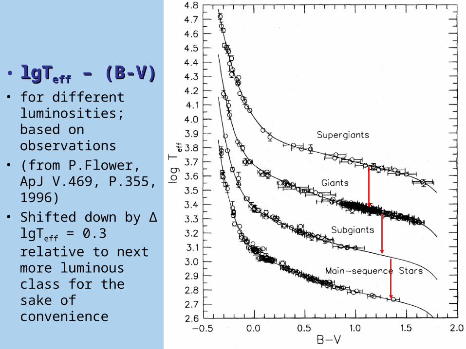
• lgTlgTeffeff – (B-V) – (B-V)• for different

luminosities; based on observations

• (from P.Flower, ApJ V.469, P.355, 1996)

• Shifted down by Δ lgTeff = 0.3 relative to next more luminous class for the sake of convenience

• T.Lejeune et al. (A&AS V.130, P.65, 1998):T.Lejeune et al. (A&AS V.130, P.65, 1998):• Colors from UV to NIR vs TColors from UV to NIR vs Teffeff (theory and empirical corrections)(theory and empirical corrections)

• Before HIPPARCOS mission, astronomers used Hyades “convergent-point” distance as most reliable zero-point of the ZAMS calibration and the base of the distance scale of all open clusters

• Recently, the situation has changed, but Hyades, along with other ~10 well-studied nearby open clusters, still play important role in the calibration of isochrones via their accurate distances

Revised HIPPARCOS parallaxes of Revised HIPPARCOS parallaxes of nearby open clusters (van Leeuwen, nearby open clusters (van Leeuwen,

2007)2007)ClusterCluster Parallax, Parallax,

error, error, masmas

(m-M)(m-M)00 and its and its error, error, magn.magn.

[Fe/H][Fe/H] Age, Age, MyrMyr

E(B-V)E(B-V)

Praesepe 5.49±0.19 6.30±0.07 +0.11 ~830 0.00

Coma Ber

11.53±0.12

4.69±0.02 -0.065 ~450 0.00

Pleiades 8.18±0.13 5.44±0.03 +0.026 100 0.04

IC 2391 6.78±0.13 5.85±0.04 -0.040 30 0.01

IC 2602 6.64±0.09 5.89±0.03 -0.020 30 0.04

NGC 2451

5.39±0.11 6.34±0.04 -0.45 ~70 0.055

α Per 5.63±0.09 6.25±0.04 +0.061 50 0.09

Hyades 21.51±0.14

3.34±0.02 +0.13 650 0.003

• Combined MMHpHp – (V-I) – (V-I) HRD for 8 nearby open clusters constructed by revised HIPPARCOS parallaxes of individual stars (from van Leeuwen, 2007) and corrected for small light extinction

• Hyades MS shift (red red squaressquares) is due to– Larger [Fe/H]– Larger age ~650 Myr

• Bottom envelope (--------) can be treated as an observed ZAMS(V-I)

MH

p

Pleiades problem:HST gives smallerparallax (by ~8%) ΔMHp ≈ -0.17m

• (a) Observed ZAMS (in absolute magnitudes) can be derived as the bottom envelope of composite CMD, constructed for well-studied open clusters of different ages but similar chemical composition

• (b) Isochrones of different ages are appended to ZAMS and “calibrated”

Primary empirical calibration of the Hyades MS & isochrone for different colors, by HIPPARCOS parallaxes

(M.Pinsonneault et al. ApJ V.600, P.946, 2004)Solid line: theoretical isochrone withLejeune et al. (A&AS V.130, P.65, 1998)color-temperature calibrations

MV

ZAMS and Hyades isochrones: sensitivity to ZAMS and Hyades isochrones: sensitivity to the age for 650±100 Myr (from Y.Lebreton, the age for 650±100 Myr (from Y.Lebreton,

2001)2001)• Fitting

color of the turn-off point

ZAMS

• Best library of isochrones recommended to calculate cluster distances, ages and extinctions:

• L.Girardi et al. “Theoretical isochrones in several L.Girardi et al. “Theoretical isochrones in several photometric systems I. (A&A V.391, P.195, 2002)photometric systems I. (A&A V.391, P.195, 2002)

• Theoretical background:Theoretical background:– (a) Evolution tracks calculations for different

initial stellar masses (0.15-7MSun) and metallicities (-2.5…+0.5) (also including α-element enhanced models and overshooting)

– (b) Synthetic spectra by Kurucz ATLAS9 – (c) Synthetic photometry (bolometric

corrections and color-temperature relations) calibrated by well-studied spectroscopic standards

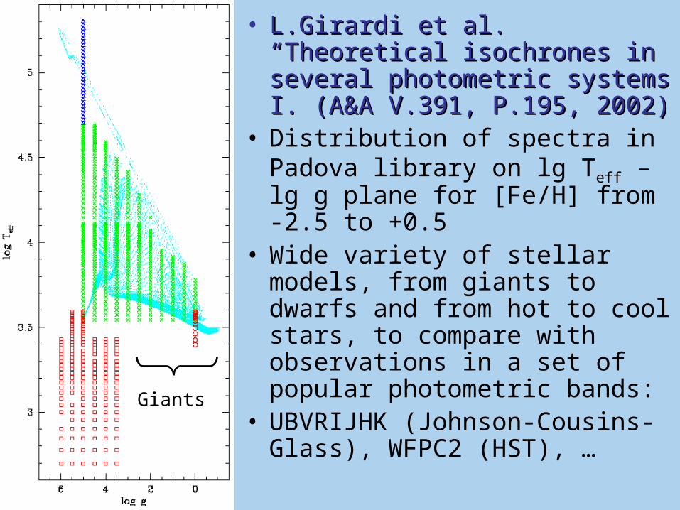
• L.Girardi et al. “Theoretical L.Girardi et al. “Theoretical isochrones in several isochrones in several photometric systems I. (A&A photometric systems I. (A&A V.391, P.195, 2002)V.391, P.195, 2002)

• Distribution of spectra in Padova library on lg Teff – lg g plane for [Fe/H] from -2.5 to +0.5

• Wide variety of stellar models, from giants to dwarfs and from hot to cool stars, to compare with observations in a set of popular photometric bands:

• UBVRIJHK (Johnson-Cousins-Glass), WFPC2 (HST), …

Giants

• Ages of open clusters vary from few Myr to ~8-10 Gyr, age of the disk

• For most clusters, [Fe/H] varies approximately from -0.5 to +0.5

• Necessary step in the distance and age determination – account for differences in metallicity ([Fe/H] or Z)

Metallicity effects on isochrones:Metallicity effects on isochrones:modelling variables, Mmodelling variables, Mbolbol - T - Teffeff

Turn-off point

Metallicity effects on isochrones: opticsMetallicity effects on isochrones: optics

Turn-off point

Metallicity effects on isochrones: NIRMetallicity effects on isochrones: NIR

Turn-off point

• The corrections ΔM and ΔCI (CI –Color Index) vs Δ[Fe/H] or ΔZ to isochrones, taken for solar abundance, can be found either– from theoretical calculations,– or empirically, by comparing multicolor photometric data for clusters with different abundances and with very accurate trigonometric distances

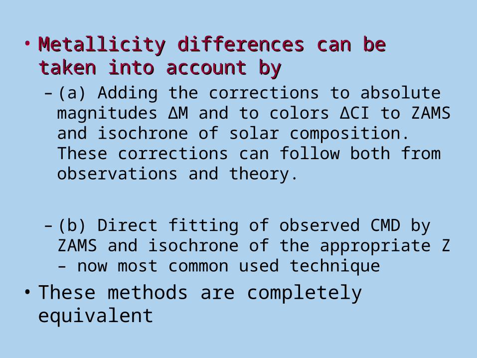
• Metallicity differences can be taken Metallicity differences can be taken into account byinto account by– (a) Adding the corrections to absolute

magnitudes ΔM and to colors ΔCI to ZAMS and isochrone of solar composition. These corrections can follow both from observations and theory.

– (b) Direct fitting of observed CMD by ZAMS and isochrone of the appropriate Z – now most common used technique

• These methods are completely equivalent

• Ideally, we should estimate [Fe/H] (or Z) prior prior to fitting CMD by isochrones

• If it is not the case, systematic errors in distances (again errors!) may result

• Open question:Open question: differences in Helium content (Y). Theoretically, can play important role. As a rule, evolutionary tracks and isochrones of solar Helium abundance (Y=0.27-0.29) are used

• L.GirardiL.Girardi et al. (2002) database on isochrones and evolutionary tracks is of great value – it provides us with “ready-to-use” multicolor isochrones for a large variety of the parameters involved (age, [Fe/H], [α/Fe], convection,…)

• Example:Example: Normalized transmission curves for two realizations of popular UBVRIJHK systems as compared to SED (spectral energy distributions) of some stars (from L.GirardiL.Girardi et al., 2002)

• See next slides for ZAMS and some isochrones

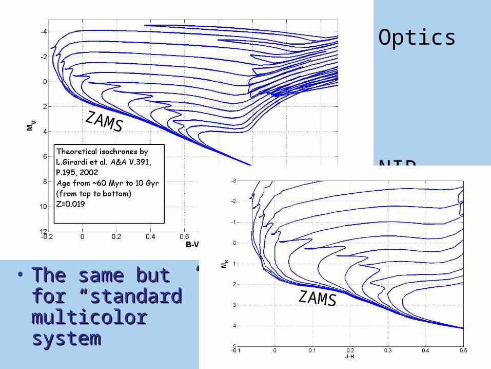
• Theoretical isochrones (color - MV magnitude diagrams) for solar composition (Z=0.019) and cluster ages 0.1 Gyr, 1 Gyr and 10 Gyr (L.GirardiL.Girardi et al., 2002, green solid lines)

0.1

1

10 Gyr

• Theoretical isochrones (NIR color-magnitude diagrams) for solar composition (Z=0.019) and cluster ages 0.1 Gyr, 1 Gyr and 10 Gyr (L.GirardiL.Girardi et al., 2002, green solid lines)

0.1

1

1 GyrWhat are fancy shapes !What are fancy shapes !

Girardi et al. isochrones in modelling Girardi et al. isochrones in modelling variablesvariables

MMbolbol – lg T – lg Teff eff (more detailed age grid)(more detailed age grid)

ZAMS

Optics

NIR

• The same but The same but for “standard” for “standard” multicolor multicolor systemsystem

ZAMS

ZAMS

How estimate age, extinction and the How estimate age, extinction and the distance?distance?11stst variant variant

• (a) Calculate color-excess CE for cluster stars on two-color diagram like (U-B) – (B-V). Statistically more accurate than for single star. Highly desirable to use a set of two-color diagrams as (U-B) – (B-V) and (B-V) – (V-I) etc., to reduce statistical and systematical errors

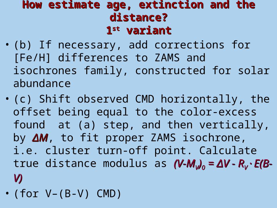
How estimate age, extinction and the How estimate age, extinction and the distance?distance?11stst variant variant

• (b) If necessary, add corrections for [Fe/H] differences to ZAMS and isochrones family, constructed for solar abundance

• (c) Shift observed CMD horizontally, the offset being equal to the color-excess found at (a) step, and then vertically, by ΔΔMM, to fit proper ZAMS isochrone, i.e. cluster turn-off point. Calculate true distance modulus as (V-M(V-MVV))00 = = ΔΔV - RV - RVV∙E(B-∙E(B-V)V)

• (for V–(B-V) CMD)

How estimate age, extinction and the How estimate age, extinction and the distance?distance?22ndnd variant variant• (a) If necessary, add corrections for [Fe/H]

differences to ZAMS and isochrones family, constructed for solar metallicity

• (b) Match observed cluster CMD (color-magnitude diagram) to ZAMS and isochrone trying to fit cluster turn-off point

• (c) Calculate hhorizontal and vvertical offsets: HH: Δ (color) = CE (color excess)

VV: (m-M) = (m-M)0 + R· CE

(m-M)(m-M)00 – true distance – true distance modulusmodulus

How estimate age, extinction and the How estimate age, extinction and the distance?distance?22ndnd variant variant

• (d) Make the same procedure for all available observations in other photometric bands

• (e) Compare all (m-M)0 and CE ratios. For MS fitting performed properly,– distances will be in general agreement,– CE ratios will be in agreement with accepted

“standard” extinction law

You can start writing paper !

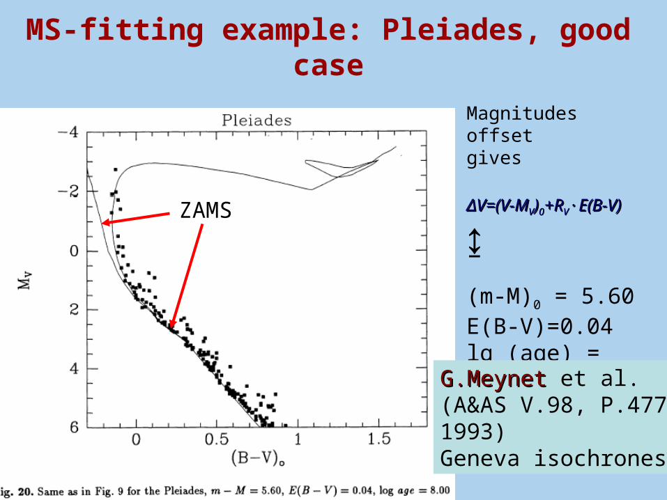
MS-fitting example: Pleiades, good case

Magnitudes offsetgives

ΔΔV=(V-MV=(V-MVV))00+R+RVV∙E(B-V)∙E(B-V)

↨(m-M)0 = 5.60E(B-V)=0.04lg (age) = 8.00

ZAMS

G.MeynetG.Meynet et al.(A&AS V.98, P.477,1993)Geneva isochrones

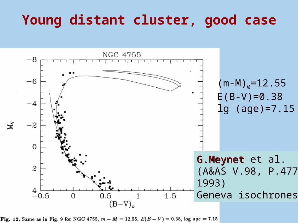
Young distant cluster, good case

(m-M)0=12.55E(B-V)=0.38lg (age)=7.15

G.MeynetG.Meynet et al.(A&AS V.98, P.477,1993)Geneva isochrones

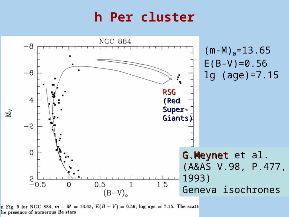
h Per cluster

RSGRSG(Red(RedSuper-Super-Giants)Giants)

(m-M)0=13.65E(B-V)=0.56lg (age)=7.15

G.MeynetG.Meynet et al.(A&AS V.98, P.477,1993)Geneva isochrones

RSGRSG

(m-M)0=12.10E(B-V)=0.32lg (age)=8.22

G.MeynetG.Meynet et al.(A&AS V.98, P.477,1993)Geneva isochrones

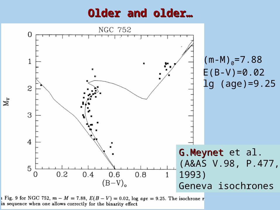
Older and older…Older and older…

(m-M)0=7.88E(B-V)=0.02lg (age)=9.25

G.MeynetG.Meynet et al.(A&AS V.98, P.477,1993)Geneva isochrones

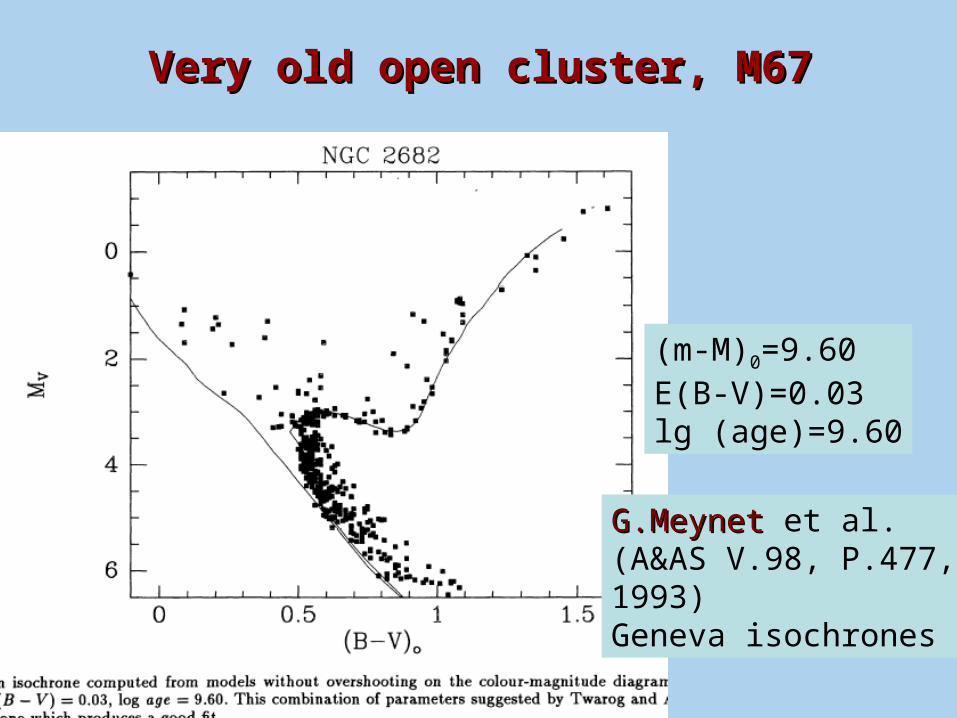
Very old open cluster, M67Very old open cluster, M67

(m-M)0=9.60E(B-V)=0.03lg (age)=9.60

G.MeynetG.Meynet et al.(A&AS V.98, P.477,1993)Geneva isochrones

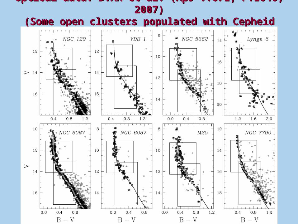
Optical data: D.An et al. (ApJ V.671, P.1640, 2007)Optical data: D.An et al. (ApJ V.671, P.1640, 2007)(Some open clusters populated with Cepheid (Some open clusters populated with Cepheid

variables)variables)

The same, NIR data: D.An et al. (ApJ The same, NIR data: D.An et al. (ApJ V.671, P.1640, 2007)V.671, P.1640, 2007)

• New parameters of open clusters populated with Cepheid variables (from D.AnD.An et al., 2007)

• The consequences for calibration of the Cepheids luminosities will be considered later

• Important note:Important note: Open cluster field is often contaminated by large amount of foreground and background stars, nearby as well as more distant non-members

• Prior to “MS-fitting” it is urgently recommended to “clean” CMD for field stars contribution, say, by selecting stars with similar proper motions on μx - μy vector-point diagram:

(kinematic selection; reason – small velocity dispersion)

Field stars

Cluster stars

MS-fitting accuracyMS-fitting accuracy(best case, multicolor photometry)(best case, multicolor photometry)(D.An et al ApJ V.655, P.233, 2007)(D.An et al ApJ V.655, P.233, 2007)

• Random error of MS-fitting– with spectroscopic [Fe/H]: δδ(m-M)(m-M)00 ≈ ±0.02 ≈ ±0.02mm, i.e

~ 1% in the distance

• Systematic errors due to uncertainties of calibrations, [Fe/H] and α-elements, field contamination and contribution of unresolved binaries– δδ(m-M)(m-M)00 ≈ ±0.04-0.06 ≈ ±0.04-0.06mm, i.e. 2-4% in the distance

• Uncertainties of Helium abundance may result in even larger systematic errors…

• For distant clusters, with CMD contaminated by foreground/background stars, and uncertainties in [Fe/H], errors may increase to

ΔΔ(m-M)(m-M)00≈±0.1≈±0.1mm(random) ± (random) ± 0.20.2mm(systematic)(systematic)

Typical distance accuracy of remote Typical distance accuracy of remote open clusters is ~10-15%open clusters is ~10-15%

• Isochrones fitting is equally applicable to globular clusters, but this is not the only method of the distance estimates

• Good idea to use additional horizontal branch luminosity

indicators, including RR Lyrae variablesRR Lyrae variables (with nearly constant luminosity, see later)

RR LyraeRR Lyrae

BHBBHB((EHB)EHB)

TPTP

• D.AnD.An et al. (arXiv:0808.0001v1)

• Isochrones (MS + giant branch) for globular clusters of different

[Fe/H] in (u g r i z) photometric bands (SDSS)

Å

u 3551Åg 4686År 6165Åi 7481Åz 8931Å

more metal-deficient

Isochrones fittingIsochrones fittingexample: M92example: M92

Age stepAge step 2 2 GyrGyr

Theoretical background ofTheoretical background ofthis method is quitethis method is quitestraightforwardstraightforward

Galactic Globular ClustersGalactic Globular Clustersare distant objects andare distant objects andvery difficult to study,very difficult to study,even with HSTeven with HST

Reliable photometric dataReliable photometric dataexist mostly for brightestexist mostly for brighteststars: Horizontal Branch,stars: Horizontal Branch,Red Giant Branch andRed Giant Branch andSubGiantsSubGiants

• CMD for selected galactic globular clusters (HST observations CMD for selected galactic globular clusters (HST observations of 74 GGC; of 74 GGC; G.PiottoG.Piotto et al., A&A V.391, P.945, 2002) et al., A&A V.391, P.945, 2002)

• Bad cases for MS-fitting (except NGC 6397)Bad cases for MS-fitting (except NGC 6397)

• For CMDs of globular clusters, without pronounced Main Sequence, there are other methods of age estimates, based on– magnitude difference between Horizontal

Branch and Turn-Off Point (“vertical method”)– color difference between Turn-Off Point and

Giant Granch (“horizontal” method)

• Illustration of the “vertical” and “horizontal” Illustration of the “vertical” and “horizontal” methods of age estimates of globular clustersmethods of age estimates of globular clusters

M.Salaris & M.Salaris &

S.CassisiS.Cassisi,,

““Evolution of starsEvolution of stars

and stellarand stellar

populations” populations”

(J.Wiley &(J.Wiley &

Sons, 2005)Sons, 2005)

“Horizontal” methodcalibrations:

Color offsetColor offset

vs [Fe/H]vs [Fe/H]for differentages

Gyr

Gyr

Gyr

Gyr

“Vertical” method calibrations: magnitude difference magnitude difference vs [Fe/H]vs [Fe/H] for different ages

Gyr

• In some cases isochrone fitting fails to give unique result because of multiple stellar populationsmultiple stellar populations found in most massive galactic and extragalactic globular clusters (ωω Cen: Cen: L.Bedin L.Bedin et al., ApJ V.605, L125, 2004; NGC NGC 1806 & NGC 1846 in LMC:1806 & NGC 1846 in LMC: A.MiloneA.Milone et al., arXiv:0810.2558v1)

ω Cen

NGC 1806 (LMC)

Multiple populations ?He abundancedifferences ?

Chapter SixChapter Six

Statistical parallaxesStatistical parallaxes

Astronomical backgroundAstronomical background• Statistical parallaxes provides very

powerful tool used to refinerefine luminosity calibrations of secondary “standard candles”, such as RR Lyrae variables, Cepheids, bright stars of constant luminosity, and isochrones applied for main-sequence fitting

• Statistical parallax technique involves space velocitiesspace velocities of uniform sample of objects – at first glance, it sounds as strange and unusual…

Main ideaMain idea

• To match the tangential velocities (VVT T = k r = k r μμ, proportional to distance scale of the sample of studied stars) and radial velocities VVRR (independent on the distance scale), under three-dimensional normal (ellipsoidal) distribution of the residual velocities

r

VT=k r μVR

Sun

If all accepted distances aresystematically larger (shorter)than true distances, then overestimated (underestimated)tangential velocities will generally distort the ellipsoidal distribution of residual velocities, and the velocity ellipsoids will look like

… instead of being alike and pointed to the galactic center

• One of the first attempts to calculate statistical parallax of stars has been made by E.PavlovskayaE.Pavlovskaya in the paper entitled “Mean absolute magnitude and the kinematics of RR Lyrae stars” (Variable Stars V.9, P.349, 1953)

• Her estimate <<MMVV>>RRRR ≈ +0.6 ≈ +0.6mm was widely used and kept before early 1980th and even recently, differ only slightly on modern value for metal-deficient RR Lyrae (~0.75m)

• First rigorous formulation of modern statistical parallax technique have been done by:

• S.Clube, J.DaweS.Clube, J.Dawe in “Statistical Parallaxes and the Fundamental Distance Scale-I & II” (MNRAS V.190, P.575; P.591, 1980)

• C.A.MurrayC.A.Murray in his book “Vectorial Astrometry” (Bristol: Adam Hilger, 1983)

• Modern (3D) formulation of the statistical parallax technique enables– (a) To refine the accepted distance scale

and absolute magnitude calibration used– (b) To take into account all observational

errors– (c) To calculate full set of kinematical

parameters of a given uniform stellar sample (space velocity of the Sun, rotation curve or other systemic velocity field, velocity dispersion etc.)

• Advanced matrix algebra is required, soAdvanced matrix algebra is required, so

only brief description followsonly brief description follows

• Detailed description of the 3D statistical parallax technique can be found only in A.Rastorguev’sA.Rastorguev’s (2002) electronic textbook in

• http://www.astronet.ru/db/msg/1172553

• “The application of the maximum-likelyhood technique to the determination of the Milky Way rotation curve and the kinematical parameters and distance scale of the galactic populations”

• (in russian)

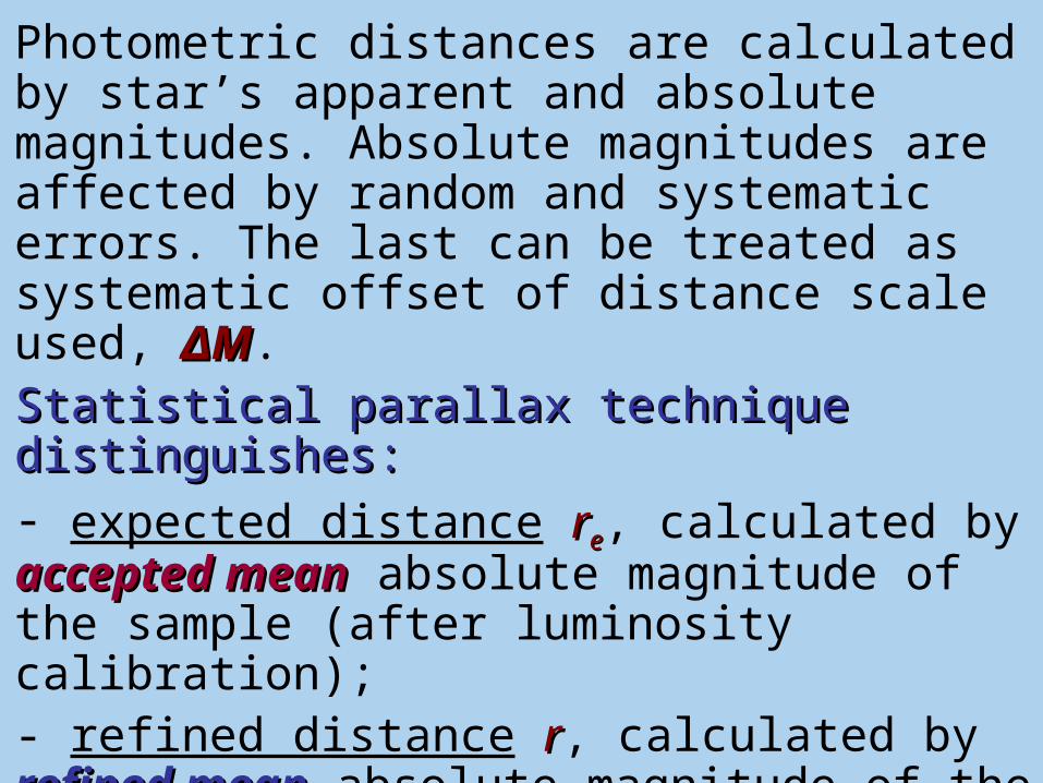
Photometric distances are calculated by star’s apparent and absolute magnitudes. Absolute magnitudes are affected by random and systematic errors. The last can be treated as systematic offset of distance scale used, ΔΔMM.Statistical parallax technique distinguishes:Statistical parallax technique distinguishes:- expected distance rree, calculated by accepted meanaccepted mean absolute magnitude of the sample (after luminosity calibration);- refined distance rr, calculated by refined refined meanmean absolute magnitude of the sample (after application of statistical parallax technique);- true distance rrtt, appropriate to truetrue absolute magnitude of the star (generally unknown).

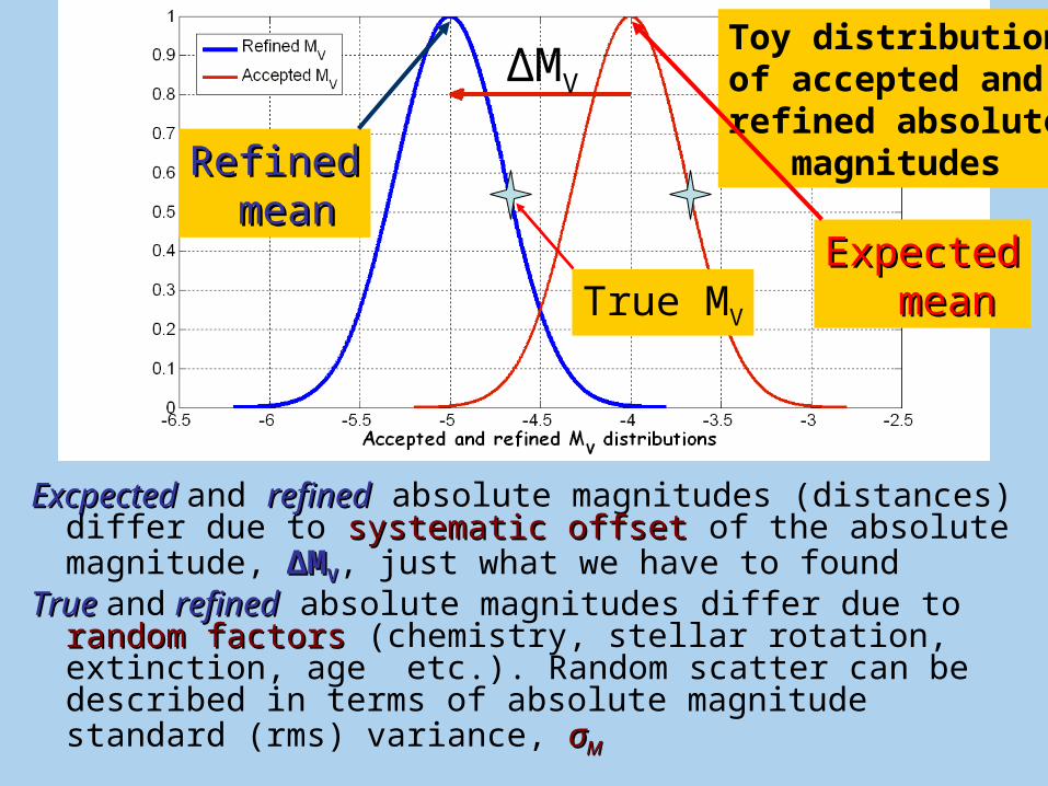
ExcpectedExcpected and refinedrefined absolute magnitudes (distances) differ due to systematic offsetsystematic offset of the absolute magnitude, ΔΔMMVV, just what we have to found

TrueTrue and refinedrefined absolute magnitudes differ due to random factorsrandom factors (chemistry, stellar rotation, extinction, age etc.). Random scatter can be described in terms of absolute magnitude standard (rms) variance, σσMM

ΔMV

Toy distributionof accepted andrefined absolute magnitudes

True MV

RefinedRefined meanmean

ExpectedExpected meanmean

Kinematic model of the stellar Kinematic model of the stellar sample:sample:

Four components of 3D-velocity:

- Local sample motionLocal sample motion relative the Sun, V0

- Systematic motionSystematic motion, including differential rotation and noncircular motions, unified by the vector VSYS

- Ellipsoidal (3D-Gaussian) distributionEllipsoidal (3D-Gaussian) distribution of true residual velocities, manifested by star’s random velocity vector η

- Errors: Errors: in radial velocity and proper motions

• Difference between “observed” space velocity and that predicted by the kinematical model is expected to have 3D-Gaussian distribution as

• where calculates for expected distance, rree

• and LL is 3x3 covariance tensor for difference

)r(V)r(VV emod,loceloc

VLVexpL)()V(f T//

12123

2

12

V

L = L = <<ΔΔV·V·ΔΔV V TT>>, , T –T – transposition sign

Vloc (re) is what we measure !

Galactic diskSun

re

Vb

Vl

VR

• VVlocloc(r(ree)) is defined in the local “astrocentric” coordinate system (see picture) via:

• VVRR radial velocity, independent on distance rree

• VVll = kr = kre e μμll velocity on the galactic longitude

• VVbb= kr= kre e μμbb velocity on the galactic latitude

After some advanced algebra:After some advanced algebra:)r(L)r(L)r(L)r(L eeresideerre

TTSSeresid P

~GLGP

~)r(L 0

]M~

GLGM~

[p.)r(L TTSSMe

0

22210

tcoefficienncorrelatio

0

0

00

22222

22222

2

bl

beblble

blblele

r

eerr

rkrk

rkrk

V

)r(L

Covariance tensor

r/)r(VP~

p/r)r(VVG[M~

syssys

00

(rotation) motion systematic,matrix ndispertsio

matrixes,dependent -coordinate known,,~

,~

0

0

sys

S

VL

GGPM

Observed errorsObserved errors

Ellipsoidal distributionEllipsoidal distribution

Systematic motion: (a) relative to the Sun and (b) rotation

where

Individual velocities of all stars are independent on each other; in this case full (N-body) distribution function is the productproduct of N individual functions ff,

where N is the number of stars, AA is the “vector” of unknown parameters to be found. Maximum Maximum Likelihood principleLikelihood principle states that observedobserved set of velocity differences is most probable of allis most probable of all possible sets. The set of parameters, AA, is calculated under assumption that FF reaches its maximum (or minimum, for maximum-likelihood functionmaximum-likelihood function LF LF )

N

iiN VfA|V...,,V,VF

121

N

iiN A|VflnA|V,...,VFlnLF

11

For 3D-Gaussian distributions functions ff, LFLF can be written as a function of AA

Here |L||L| is matrix determinant, LL-1-1 is inverse matrix. By minimizing LFLF by AA, we calculate all

important parameters {A}{A}, for example:

N

iii

Tii VLVLlnlnN)A(LF

1

1

2

12

2

3

factor scale distance17.2/1/

s parametercurverotation ,...),,(

axesellipsoid velocity ),,(

Sun the toelativevelocity r sample),,(

000

000

Mrrp

wvu

e

WVU

Robust statistical parallax method:Robust statistical parallax method:applied to local disk populationsapplied to local disk populations

Astronomical background:

AA, Oort constant, derived from proper motions alone, depends on the distance scale used, whereas AA, derived only from radial velocities, do not depend on the distances

As a result, scale factor can be estimated by requirement that both AA values are equal to each other

Local Oort’s approximation

Differential rotation contribution to space velocity components in local approximation

r << Rr << R00 ((or |R|RPP –R–R0 0 | << R| << R00 ))::

lcosbcosrRR

)lcosbcosR

r(R)lcosbcos

R

rbcos

R

r(RR

P

P

0

0

20

0

220

220

2 2121

lcosbcosr 00

To first order by the ratio r/R0 in the expansion for the angular velocity:

Differential rotation effect to radial velocity Differential rotation effect to radial velocity Vr Vr ::

locpec

T

b

l

r

V

W

V

U

G

blR

brbrlR

blR

rk

rk

V

0

0

0

00

000

00

sinsin)(

cos)(coscos

cossin)(

2

2

22

000

20

20000

RA

,bcoslsinrAV

bcoslsinR

bcoslsin)(RV

rotr

rotr

From 1st Bottlinger equation (for radial velocity)

calculate contribution of the differential rotation tocalculate contribution of the differential rotation to VVr r :

AA Oort’s constant (definition)

Linearity on r,“double wave” on l

Differential rotation effect to tangential Differential rotation effect to tangential velocity velocity VVl l ::

locpec

T

b

l

r

V

W

V

U

G

blR

brbrlR

blR

rk

rk

V

0

0

0

00

000

00

sinsin)(

cos)(coscos

cossin)(

bcosr)A(bcoslcosrAV

bcosrbcoslcosrA

bcosrbcoslcosrbcoslcosRr

bcosr))(bcosrlcosR(V

rotl

rotl

000

02

0

02

022

00

000

2

2

From 2nd Bottlinger equation (for velocity on l)

calculate contribution of the differential rotation tocalculate contribution of the differential rotation to VVl l :

Linearity on r,“double wave” on l

Oort constant Oort constant AA and the refinement of the and the refinement of the distance scaledistance scale

bcoslsinrpAV truerotr

20 2

bcos)A(bcoslcosAk

bcosr)A(bcoslcosrArkV

rotl

rotl

rotl

000

000

2

2

AA00VrVr depends on the distance scale: AA00

VrVr ~ p ~ p -1-1

(decreases with increasing distances)

AA00μμll do not depend on the distance scale, AA00

μμll ≈≈ constconst

The requirement AA00VrVr (p) (p) ≈≈ AA00

μμll – robust method of the

adjusting the scale factor pp

Illustration of the robust Illustration of the robust techniquetechnique

Optimal value ofOptimal value ofthe scale factorthe scale factor

AAVrVr

AAμμll

F.A.Q. How the corrections to F.A.Q. How the corrections to absolute magnitudes are affected absolute magnitudes are affected

by the:by the:• (a) Shape of the velocity distribution (deviation

from expected 3D-Gaussian form)• (b) Vertex deviation of the velocity ellipsoid

(velocity-position correlations)• (c) Misestimates of the observation errors• (d) Non-uniform space distribution of stars• (e) Sample size• (f) Malmquist bias (excess of intrinsically bright

stars in the magnitude-limited stellar sample)• (g) Interstellar extinction• (h) Misidentification of stellar populations

• Possible factors of systematic systematic offsetsoffsets have been analyzed by P.Popowski & A.GouldP.Popowski & A.Gould in the papers “Systematics of RR Lyrae statistical parallax. I-III” (ApJ V.506, P.259, P.271, 1998; ApJ V.508, P.844, 1998) (a) (a) analyticallyanalytically and (b) by Monte-(b) by Monte-Carlo simulations,Carlo simulations, and applied to the sample of RR Lyrae variables

P.Popowski & A.Gould P.Popowski & A.Gould (1998):(1998):

• “Statistical parallax method … is extremely robust and insensitiveextremely robust and insensitive to several different categories of systematic effects”

• “… statistical errors are dominated by the size of the stellar sample”

• … sensitive to systematic errors in the observed data

• … Malmquist bias should be taken into account prior to calculations

• To eliminate the effects due to non-uniformity of the sample, bimodal bimodal versionsversions of the statistical parallax method can be used (A.Rastorguev, A.Rastorguev, A.Dambis & M.ZabolotskikhA.Dambis & M.Zabolotskikh “The Three-Dimensional Universe with GAIA”, ESA SP-576, P.707, 2005)

• Example: RR Lyrae sample of halo and thick disk stars

• Statistical parallax technique is considered as the absolute methodthe absolute method of the distance scale calibration, though it exploits prior information on the adequate kinematic model of the sample studied

• After HIPPARCOS, luminosities and distance scales of RR Lyrae stars, Cepheids and young open clusters have been analyzed by the statistical parallax technique